Advanced Performance Modeling andAnalysis

Miklos TelekDepartment of Telecommunications

Technical University of Budapest

e-mail: telek@hit.bme.hu

July 3, 2019.

Outline• Non-Markovian queues

– M/G/1, G/M/m, G/G/1 queues

• Matrix geometric methods– Phase type distributions– Markov arrival process– Quasi birth-death processes– Solution methods

• Fluid queues– Types (infinite/finite, first/second or-

der, homogeneous/inhomogeneous)– Spectral and diff. eq. based solutions– Matrix analytic solution

1

Syllabus: Probability

CDF: F (t) = Pr(X ≤ t),

PDF: f(t) =d

dtF (t),

Hazard rate – intensity: λ(t) =f(t)

1− F (t),

Expectation: E(G(X)) =

∫t

G(t) dF (t)

Moments: E(Xn) =

∫t

tn dF (t)

Laplace transform: F∼(s) = E(e−sX) =

∫t

e−st dF (t)

Z transform: N(z) = E(zN) =∑i

pizi

2

Syllabus: Properties of transforms

The distribution of a r.v. is uniquely defined by

• Distribution function (or PDF, PMF)

• Transform (Laplace, z, moment generating func-tion E(eXθ))

• Series of moments (if∞∑n=1

12n√E(Xn)

=∞)

3

Syllabus: Moments and transforms

Relation of moments and transforms:

• moment generating function:

E(eXθ) = E

( ∞∑n=0

(Xθ)n

n!

)=

∞∑n=0

E(Xn)θn

n!

−→ E(Xn) =dn

dθnE(eXθ)

∣∣∣∣θ=0

• Laplace transform:

dn

dsnf∗(s)

∣∣∣∣s=0

=dn

dsn

∫t

e−stf(t)dt

∣∣∣∣s=0

=

∫t

(−t)ne−stf(t)dt

∣∣∣∣s=0

= (−1)n∫t

tnf(t)dt

−→ E(Xn) = (−1)ndn

dsnf∗(s)

∣∣∣∣s=0

4

Syllabus: Moments and transforms

Relation of moments and transforms:

• z transform

dn

dznN(z)

∣∣∣∣z=1

=dn

dzn

∞∑i=0

pi zi

∣∣∣∣z=1

=

∞∑i=0

pi i(i− 1) . . . (i− n+ 1)zi−n∣∣∣∣z=1

=∞∑i=n

pii!

(i− n)!

Factorial moments:

−→ E(X(X − 1) . . . (X − n+ 1)) =dn

dznN(z)

∣∣∣∣z=1

5

Syllabus: Conditional probability

Conditional probability: Pr(A|B) =Pr(AB)

Pr(B),

Unconditioning (total probability):

Pr(A) =∑i

Pr(A|Bi)Pr(Bi) where∑i

Pr(Bi) = 1

Pr(A) =

∫x

Pr(A|x)dF (x) where

∫x

dF (x) = 1

6

Syllabus: Continuous distributions

Exponential distribution:

f(t) = λe−λt, F (t) = 1− e−λt, λ(t) = λ,

E(X) =1

λ, c2 =

σ2(X)

E2(X)=E(X2)− E2(X)

E2(X)= 1.

F∼(s) = E(e−sX) =

∫t

e−stdF (t) =λ

s+ λ

Erlang(n) distribution:

f(t) =λ(λt)n−1

(n− 1)!e−λt, E(X) =

n

λ, F∼(s) =

(λ

s+ λ

)n.

7

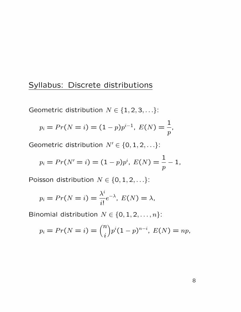
Syllabus: Discrete distributions

Geometric distribution N ∈ 1,2,3, . . .:

pi = Pr(N = i) = (1− p)pi−1, E(N) =1

p,

Geometric distribution N ′ ∈ 0,1,2, . . .:

pi = Pr(N ′ = i) = (1− p)pi, E(N) =1

p− 1,

Poisson distribution N ∈ 0,1,2, . . .:

pi = Pr(N = i) =λi

i!e−λ, E(N) = λ,

Binomial distribution N ∈ 0,1,2, . . . , n:

pi = Pr(N = i) =(ni

)pi(1− p)n−i, E(N) = np,

8

Syllabus: Poisson process

3 identical representations:

• short term behaviour:

Pr(0 arrival in (t, t+ δ)) = 1− λδ + σ(δ)

Pr(1 arrival in (t, t+ δ)) = λδ + σ(δ)

Pr(more than 1 arrivals in(t, t+ δ)) = σ(δ)

• inter-arrival time:

inter-arrival periods are independent and exponen-tially distributed with parameter λ

→ time to the nth is Erlang(n) distributed.

• arrivals in t long interval:

number of arrivals in any t long interval is Poissondistributed with parameter λt

Pr(k arrivals in (u, u+ t)) =(λt)k

k!e−λt

9

Syllabus: Basic rules

Sum of discrete random variables (Z = X + Y ):

zi =∑k

xkyi−k, Z(z) = X(z)Y (z)

Sum of continuous random variables (Z = X + Y ):

fZ(t) =

∫x

fX(x)fY (t− x)dx, F∼Z (s) = F∼X(s)F∼Y (s)

Sum of random variables (Z = X + Y ):

FZ(t) =

∫x

FX(t− x)dFY (x), F∼Z (s) = F∼X(s)F∼Y (s)

Remaining lifetime:

Fτ(t) = Pr(X − τ < t|X > τ) =F (t+ τ)− F (τ)

1− F (τ)

Equilibrium distribution of X:

f(t) =1− FX(t)

E(X), E(Y n) =

E(Xn+1)

(n+ 1)E(X)

10

Syllabus: Properties of distribution

Ageless distribution:

λ(t) is constant→ exponential distribution, c2 = 1

Aging distributions:

λ(t) is increasing→ e.g., Erlang(n) distribution, c2 < 1

Deaging distributions:

λ(t) is decreasing→ e.g., Hyper-exponential distribution, c2 > 1

11

Syllabus: Semi-Markov process

Time homogeneous discrete state continuous time stochas-tic process (X(t)) which is memoryless at state transi-tion epochs (T0 = 0, T1, T2, . . .).

Kernel Kij(t) = Pr(T1 < t,X(T1) = j|X(0) = i) de-scribes the joint distribution of the next state and thetime spent in the current state.

The state of the process at state transitions form an“embedded” DTMC X(T0), X(T1), X(T2), X(T3), . . ..

The state transition probability matrix of the embeddedDTMC is P = K(∞). Let the stationary distribution ofthe embedded DTMC be π, that is πP = π, π1I = 1.

The distribution of time spent in state i is Ki(t).

=Pr(T1 < t|X(0) = i) =

∑jKij(t) and its mean is τi =

E(T1|X(0) = i) =∫t1−Ki(t)dt.

Transient distribution

zi = limT→∞

Pr(X(T ) = i) =πiτi∑j πjτj

12

Syllabus: Semi-Markov process

Based on the ergodicity of semi-Markov processes wecan write

zi = limT→∞

Pr(X(T ) = i) = limT→∞

1

T

∫ T

t=0IX(t)=idt

= limN→∞

1

TN

∫ TN

t=0IX(t)=idt

= limN→∞

1

TN

N∑k=1

∫ Tk

t=Tk−1

IX(t)=idt

= limN→∞

1

TN

N∑k=1

IX(Tk−1)=i(Tk − Tk−1|X(Tk−1) = i)

= limN→∞

N∑k=1

IX(Tk−1)=i(Tk − Tk−1|X(Tk−1) = i)︸ ︷︷ ︸→Nπiτi∑

j

N∑k=1

IX(Tk−1)=j(Tk − Tk−1|X(Tk−1) = j)︸ ︷︷ ︸→Nπjτj

=πiτi∑j πjτj

13

Syllabus: Markov regenerative process

Time homogeneous discrete state continuous time stochas-tic process (X(t)) which is memoryless at some instanceof time (T0 = 0, T1, T2, . . .).

The global kernel, Kij(t) = Pr(T1 < t,X(T1) = j|X(0) =i), describes the joint distribution of the state at thenext memoryless instance and the time to the next mem-oryless instance.

The process behaviour between memoryless instancesis described the local kernel Eij(t) = Pr(T1 > t,X(t) =j|X(0) = i).

The state of the process at memoryless instances forman “embedded” DTMC X(T0), X(T1), X(T2), X(T3), . . ..

The state transition probability matrix of the embeddedDTMC is P = K(∞). Let the stationary distribution ofthe embedded DTMC be π, that is πP = π, π1I = 1.

During a regenerative period starting from i the meantime spent in state j is τij =

∫tEij(t)dt.

Transient distribution

zi = limT→∞

Pr(X(T ) = i) =

∑j πjτj,i∑

j

∑k πjτj,k

14

Syllabus: Markov regenerative process

Based on the ergodicity of Markov regenerative pro-cesses we can write

zi = limT→∞

Pr(X(T ) = i) = limT→∞

1

T

∫ T

t=0IX(t)=idt

= limN→∞

1

TN

∫ TN

t=0IX(t)=idt

= limN→∞

1

TN

N∑k=1

∫ Tk

t=Tk−1

IX(t)=idt

= limN→∞

1

TN

∑j

N∑k=1

IX(Tk−1)=j

∫ Tk

t=Tk−1

IX(t)=i|X(Tk−1)=jdt

= limN→∞

∑j

N∑k=1

IX(Tk−1)=j

∫ Tk

t=Tk−1

IX(t)=i|X(Tk−1)=jdt︸ ︷︷ ︸→Nπjτji∑

j

∑k

N∑k=1

IX(Tk−1)=j

∫ Tk

t=Tk−1

IX(t)=k|X(Tk−1)=jdt︸ ︷︷ ︸→Nπjτjk

=

∑j πjτji∑

j

∑k πjτj,k

15

M/G/1 queue

Poisson arrival process, general service time distribution,one server, infinite buffer, FIFO.

→ X(t) is not a CTMC.

System behaviour depends on elapsed service time ofcustomer under service.

Memoryless instances: e.g. departure instances.

→ embedded Discrete time Markov chain

Notations:

λ arrival rate, B service time r.v. (TB = E(B)),

Q queue length r.v., W waiting time r.v.,

W0 remaining service time r.v.

16

M/G/1 queue: mean queue length

Server utilization: ρ = λTB

Mean waiting time:

W = W0 +Q TB

Little’s law (Q = λW ) →

W =W0

1− ρRemaining service time of customer under service:

W0 = P (server busy) R+ P (server idle) 0 = ρ R

Remaining service time of busy server:

R =T 2B

2TB=TB

2(1 + c2

B)

Applying Little’s law again →

Q = λW =ρ2(1 + c2

B)

2(1− ρ)

Pollaczek-Khinchin formulae for mean queue length.

17

M/G/1 queue: mean queue length

Mean queue length (Q) versus utilization (ρ) with c2B =

0.5,1,2

0.75 0.8 0.85 0.9 0.95

5

10

15

20

25

18

M/G/1 queue: stationary distribution

DTMC embedded in departure epochs:

Xn number of customers after the nth departure

Xn+1 =

Xn − 1 + Y, if Xn > 0Y, if Xn = 0

Xn+1 = (Xn − 1)+ + Y

Transition probability matrix:

P =

a0 a1 a2 · · ·a0 a1 a2 · · ·0 a0 a1 · · ·0 0 a1 · · ·... ... ... . . .

The number of customer arrives during a service period:

ak = P (k customer arrives) =

∫ ∞0

e−λt(λt)k

k!dB(t)

19

M/G/1 queue: stationary distribution

Balance equations of the embedded DTMC:

ν0 = ν0a0 + ν1a0

νk = ν0ak +k+1∑i=1

νiak−i+1, k ≥ 1

Multiplying the kth equation by zk and summing up re-sults:

G(z) =∞∑k=0

νkzk = ν0GA(z) +

1

z(G(z)− ν0)GA(z),

where

GA(z) =∞∑k=0

akzk = . . .

=

∫ ∞t=0

e−λt(1−z)dB(t) = B∼(λ(1− z))

Pollaczek-Khinchin formulae for queue length distribu-tion:

G(z) = ν0(z − 1)B∼(λ(1− z))

z −B∼(λ(1− z))

20

M/G/1 queue: busy period

1H2H

3

2

1

s54 7sss3s s6

7

s1 2

T6T53 T T4T2

t

U(t)

T1T0T

The number of customer served between a departurewith n customers and the first time with n−1 customersis Qn.

First time to have n−1 customers in the system startingfrom a departure with n customers is Hn.

Due to the regular “level independent” structure of theM/G/1 queue and matrix P Hn and Qn are independentof n !!!

21

M/G/1 queue: busy period

The number of customers arrive during the service timesuppose that B = τ is Poisson distributed with λτ .

The conditional distribution of the busy period is

H|B = τ =

τ eλτ

τ +H1 λτeλτ

τ +H2 +H1(λτ)2

2!eλτ

. . .

Using h∗(s) = E(e−sH) = h∗1(s) = h∗2(s) = . . . we have

E(e−sH|B = τ) =∞∑i=0

(λτ)i

i!e−λτe−sτ(h∗(s))i

= e−λτe−sτeλτh∗(s) = e−τ(s+λ−λh∗(s))

and

h∗(s) =

∫ ∞τ=0

E(e−sH|B = τ)b(τ)dτ =

=

∫ ∞τ=0

e−τ(s+λ−λh∗(s))b(τ)dτ =

= b∗(s+ λ− λh∗(s))

22

M/G/1 queue: busy period

Similarly the conditional distribution of the number ofcustomers served in busy period is

Q|B = τ =

1 eλτ

1 +Q1 λτeλτ

1 +Q2 +Q1(λτ)2

2!eλτ

. . .

Using Q(z) = E(zQ) = Q1(z) = Q2(z) = . . . it is

E(zQ|B = τ) = z

∞∑i=0

(λτ)i

i!e−λτQ(z)i

= z e−λτeλτQ(z) = z e−τ(λ−λQ(z))

and

Q(z) =

∫ ∞τ=0

E(zQ|B = τ)b(τ)dτ =

=

∫ ∞τ=0

z e−τ(λ−λQ(z))b(τ)dτ =

= z b∗(λ(1−Q(z)))

23

M/G/1 queue: busy period

The moments of H and Q can be obtained from h∗(s)and Q(z). E.g.,

E(H) = −d

dsh∗(s)|s=0

= −b∗′(s+ λ− λh∗(s))(1− λh∗′(s))|s=0

= −b∗′(0)(1− λh∗′(0)) = TB(1 + λE(H))

=TB

1− ρ.

Since ρ = λTB.

24

M/G/1 queue: busy period

But they can be calculated directly as well:

E(H|B = τ) = τ +∞∑i=0

(λτ)i

i!e−λτ iE(H) = τ + λτE(H)

and

E(H) =

∫ ∞τ=0

E(H|B = τ)b(τ)dτ

= (1 + λE(H))

∫ ∞τ=0

τb(τ)dτ

= (1 + λE(H))TB

=TB

1− ρ.

Similarly

E(Q) =1

1− ρ.

25

M/G/1 queue: special cases

M/M/1 queue: B∼(s) =µ

s+ µ, c2

B = 1

Q =ρ2

1− ρ

G(z) = ν01

1− ρz=

1− ρ1− ρz

νk = ν0ρk = (1− ρ)ρk

M/D/1 queue: B∼(s) = e−sD, c2B = 0, (ρ = λD)

Q =ρ2

2(1− ρ)

G(z) = ν0z − 1

zeρ(1−z) − 1

26

M/G/1 queue as Markov regenerative process

X(t) is the number of customers at time t. There areembedded time points, T0, T1, . . ., at customer depar-tures. The global and local kernels are

Kij(t) = Pr(T1 < t,X(T1) = j|X(0) = i),

Eij(t) = Pr(T1 > t,X(t) = j|X(0) = i).

i = 1:

K1k(t) = Pr(B < t, k arrivals in (0, B))

=

∫ t

τ=0

(λτ)k

k!e−λτdB(τ), k ≥ 0,

E1k(t) = Pr(B > t, k − 1 arrivals in (0, t))

=(λt)k−1

(k − 1)!e−λt (1−B(t)), k ≥ 1,

27

M/G/1 queue as Markov regenerative process

i = 0:

E00(t) = Pr(0 arrival in (0, t)) = e−λt

first arrival at τ and a service period starting from 1:

E0j(t) =

∫ t

τ=0λe−λτE1j(t− τ)dτ, j ≥ 1,

K0j(t) =

∫ t

τ=0λe−λτK1j(t− τ)dτ, j ≥ 0,

i > 1:

Kij(t) =

K1,j−i+1(t), if i ≥ 1, j ≥ i− 1,

0, othervise.

Eij(t) =

E1,j−i+1(t), if i ≥ 1, j ≥ i,

0, othervise.

Exercise: relation of the embedded and the stationary

distribution based on this MRP representation.

28

G/M/1 queue

Renewal arrival process (i.i.d. inter-arrival times), ex-ponentially distributed service time, m server, infinitebuffer, FIFO.

→ X(t) is not a CTMC.

System behaviour depends on the time elapsed since thelast arrival.

Memoryless instances: arrival instances.

→ embedded Discrete time Markov chain

29

Special case: G/M/1 queue

DTMC embedded in arrival epochs:

Xn number of customers before the nth arrival

Xn+1 = Xn + 1− Y ′ = (Xn + 1− Y )+

where

• Y ′ number of customer served between the nth andn+ 1th arrivals,

• Y number of Poisson(µ) instances between the nthand n+ 1th arrivals.

30

Special case: G/M/1 queue

Transition probability matrix:

P =

c0 b0 0 0 · · ·c1 b1 b0 0 · · ·c2 b2 b1 b0 · · ·c3 b3 b2 b1 · · ·... ... ... ... . . .

The number of Poisson(µ) instances during an inter-arrival period:

bk =

∫ ∞0

e−µt(µt)k

k!dA(t)

The more than k Poisson(µ) instances during an inter-arrival period:

ck =∞∑

i=k+1

bi

31

G/M/m queue

Server utilization is ρ =λ

mµ,

where λ is the mean arrival rate.

Transition probability matrix:

P =

p00 p01 0 · · · 0 0 · · ·p10 p11 p12 · · · 0 0 · · ·p20 p21 p22 · · · 0 0 · · ·

... ... ... 0 0 · · ·pm−1,0 pm−1,1 pm−1,2 · · · b0 0 · · ·pm,0 pm,1 pm,2 · · · b1 b0 · · ·pm+1,0 pm+1,1 pm+1,2 · · · b2 b1 · · ·

... ... ... ... ... . . .

Number of services when all servers are busy:

bk =

∫ ∞0

e−mµt(mµt)k

k!dA(t)

32

G/M/m queue

After an arrival i+ 1 ≤ m customers:all customers are under servicei− j + 1 complete service, j do not:

pi,j =

∫ ∞0

( i+ 1

i− j + 1

)(1− e−µt)i−j+1e−µtjdA(t)

After the arrival i+ 1 > m customers:i−m+ 1 customers are in queue, m under service.τ : time to empty the queue

(Erlang(i-m+1) distribution)

pi,j =

∫ ∞t=0

∫ t

x=0

(mj

)(1− e−µ(t−x))m−je−µ(t−x)jfτ(x)dxdA(t)

where τ is Erlang(i−m+ 1,mµ), that is

fτ(x) =mµ(mµx)i−m

(i−m)!e−mµx.

33

G/M/m queue: stationary distribution

Conjecture: geometric stationary distribution

ν0, ν1, . . . , νm−2, κσm−1, κσm, κσm+1, . . .

Verification (k ≥ m):

νk = νk−1b0 + νkb1 + . . . =∞∑

i=k−1

νibi−k+1

Using νk = κσk: κσk =∞∑

i=k−1

κσibi−k+1

Hence

σ =∞∑i=0

σibi =

∫ ∞0

e−mµt∞∑i=0

(σmµt)i

i!dA(t) =∫ ∞

0e−(mµ−mµσ)t dA(t) = A∼(mµ−mµσ),

that is

σ = A∼(mµ−mµσ).

The ν0, ν1, . . . , νm−2 state probabilities and κ are obtained

from the linear system of the first m equations.

34

G/M/m queue: waiting time

Probability of queueing an arriving customer:

Pr(queueing) =∞∑i=m

νi =∞∑i=m

κσi =κσm

1− σ

Queue length distribution (prior to arrival) if arrivingcustomer joints queue:

Pr(Q = k|queueing) =κσm+k

κσm

1−σ= (1− σ)σk

Waiting time distribution if n − m customers enqueueprior to arrival:

W∼(s|n−m) =

(mµ

s+mµ

)n−m+1

Waiting time distribution if the customers queues:

W∼(s|queueing) =∞∑

n=m

W∼(s|n−m)Pr(Q = n−m|queueing) =

(1− σ)mµ

s+ (1− σ)mµ

Exponentially distributed with parameter (1− σ)mµ.

35

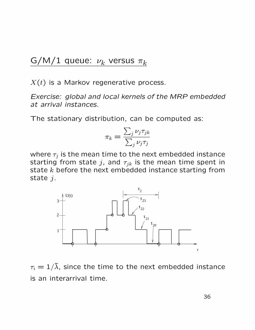
G/M/1 queue: νk versus πk

X(t) is a Markov regenerative process.

Exercise: global and local kernels of the MRP embeddedat arrival instances.

The stationary distribution, can be computed as:

πk =

∑j νjτjk∑j νjτj

where τj is the mean time to the next embedded instancestarting from state j, and τjk is the mean time spent instate k before the next embedded instance starting fromstate j.

τ21τ

22

20

τ23

τ2

τ

1

3

2

t

U(t)

τi = 1/λ, since the time to the next embedded instance

is an interarrival time.

36

G/M/1 queue: νk versus πk

21τ

1

time to arrive level 1

next departure

next arrival

τt−

τ

3

2

analysis of

time spent in level 1 before arrival or departure

U(t)

t

Analysis of τik:

τ is the sum of i+ 1− k service times

→ Erlang(i+ 1− k, ν) distribution

τik =

∫ ∞t=0

∫ t

τ=0

∫ t−τ

x=0e−µx dx fErl(i+1−k)(τ) dτ dA(t)

τi0 =

∫ ∞t=0

∫ t

τ=0(t− τ) fErl(i+1−k)(τ) dτ dA(t)

Level independent behaviour (k>0): τi,k = τi+j,k+j, ∀j

37

G/M/1 queue

Single server: m = 1→ νk = κσk = (1− σ)σk

PASTA property does not hold:

ν0 = 1− σ 6= π0 = 1− ρ = 1−λ

mµ

Indeed π0 = 1− ρ and πk = ρ(1− σ)σk−1 (k ≥ 1).

Queue parameters:

K =ρ

1− σT =

1

µ

1

1− σ

Q =ρ σ

1− σW =

1

µ

σ

1− σ

38

Special G/M/1 queues

M/M/1 queue: A∼(s) =λ

s+ λ

σ = A∼(µ− σµ) =λ

µ− σµ+ λ

σ1 =λ

µ= ρ (σ2 = 1)

E2/M/1 queue: A∼(s) =

(λ

s+ λ

)2

ρ =λ

µ=

λ

2µ, σ = 2ρ+

1

2−√

2ρ+1

4

D/M/1 queue: A∼(s) = e−sD

ρ = µD, σ = A∼(µ− σµ) = e−µD(1−σ)

H2/M/1 queue: A∼(s) =p1λ1

s+ λ1+

p2λ2

s+ λ2

p1 = p2 = 0.5, λ1 = 2λ2 = λ = 1, λ =2λ

3

ρ =λ

µ=

2λ

3µσ =

9ρ

8+

1

2−√

9ρ2

64+

1

4

39

Special G/M/1 queues

σ versus ρ

in H2/M/1, M/M/1, E2/M/1, D/M/1 queues

0.2 0.4 0.6 0.8 1

0.2

0.4

0.6

0.8

1

ρ

σ

40

Special G/M/1 queues

Relation of inter-arrival time distributions:

c2H2

= 1.22 > c2Exp = 1 > c2

E2= 0.5 > c2

Det = 0

1 2 3 4 5t

0.2

0.4

0.6

0.8

pdf

0.5 1 1.5 2 2.5 3 3.5t

0.2

0.4

0.6

0.8

1

1.2

1.4

lambda

41

G/G/1 queue

Renewal arrival process, general service time distribu-tion, one server, infinite buffer, FIFO.

→ X(t) is not a CTMC.

System behaviour depends on service time of customerunder service and the last arrival time.

42

G/G/1 queue: Unfinished work

sn service time of the nth customer,

tn+1 inter-arrival time after the nth customer.

Unfinished work, U(t): the amount of time to completethe service of customers in the system.

C n C n+1 C n+2

t

U(t)

s

ww

sn

n

n+1

n+1

n+2s

n+1 n+2t t

wn+1 =

wn + sn − tn+1 if wn + sn − tn+1 ≥ 00 otherwise

Let un = sn − tn+1

wn+1 = max(0, wn + un) = (wn + un)+

Stability condition: E(un) < 0

43

G/G/1 queue: Lindley integral equation

Distribution of un:

Cn(x) = Pr(un ≤ x) =

∫ ∞t=0

B(t+ x) dA(t)

Distribution of wn+1:

Wn+1(x) = Pr(wn+1 ≤ x) =

∫ ∞t=0−

Cn(x− t) dWn(t)

(Wn(x) = 0 for x < 0.)

Stationary behaviour (n→∞)

W (x) = Pr(w ≤ x) =

∫ ∞t=0−

C(x− t) dW (t)

Lindley integral equation

44

G/G/1 queue: Lindley integral equation

Solution of Lindley integral equation:

Spectral solution, based on A∼(s) and B∼(s).

Numerical approximation:

w1 = max(0, u0 + w0)w2 = max(0, u1 + w1) = max(0, u1, u1 + u0 + w0)w3 = max(0, u2 + w2)

= max(0, u2, u2 + u1, u2 + u1 + u0 + w0),

where un are i.i.d. random variables with E(un) < 0.

One can approximate W (x) based on a finite series, since

limn→∞

Pr

(n∑i=1

ui > 0

)= 0

45

Phase type distributions

Time to absorption in a Markov chain with N transientand 1 absorbing state.

If the Markov chain is

• CTMC→ Continuous Phase Type distribution (CPH)

• DTMC → Discrete Phase Type distribution (DPH)

Representation:

Initial probability distribution (α) + Markov chain de-scription

• CPH → generator matrix (A)

• DPH → transition probability matrix (B)

Only for transient states.

46

Properties of phase type distributions

CPH distributions:

Generator matrix: A =

[A a0 0

](a = −A1I)

PDF: f(t) = αeAta

CDF: F (t) = 1−αeAt1I

power moments: µk = k! α(−A)−k1I = k! α(−A)−k−1a

LST: f∗(s) = α(sI−A)−1a = α

[det(sI−A)jidet(sI−A)

]a

DPH distributions:

Generator matrix: B =

[B b0 1

](b = 1I−B1I)

PMF: pk = Pr(X = k) = αBk−1b

CDF: F (k) = Pr(X ≤ k) = 1−αBk1I

factorial moments: γk = k! α(I−B)−kBk−11I

z-transform: F(z) = z α(I−zB)−1b = z α

[det(I− zB)jidet(I− zB)

]b

47

Properties of phase type distributions

CPH DPH

rational Laplace tr. rational Z transform

closed for min/max, mixture, summation, ...

f(t) > 0 pi = Pr(X = i) ≥ 0

infinite support finite or infinite support

exponential tail geometric tail

CVmin =1

N> 0 CVmin = F (N,µ) ≥ 0

CVmin ↔ CVmin ↔Discrete Erlang or

Erlang distr. Determined structure

48

Operations with phase type distributions

Summation:

Z = X + Y , where X and Y are independent, X isPH(α,A) and Y is PH(β,B)

then Z is PH(γ,G) with

γ =[α 0

]

G =

[A aβ0 B

]

49

Operations with phase type distributions

Mixture:

Z =

X with probability p,Y with probability (1− p),

where X and Y are independent, X is PH(α,A) and Yis PH(β,B)

then Z is PH(γ,G) with

γ =[pα (1− p)β

]

G =

[A 00 B

]

50

Operations with phase type distributions

Minimum:

Z = Min(X,Y ), where X and Y are independent, X isPH(α,A) and Y is PH(β,B)

then Z is PH(γ,G) with

γ = α⊗ β

G = A⊕B

where

Kronecker product: A⊗

B =A11B . . . A1nB

... ...An1B . . . AnnB

Kronecker sum: A⊕

B = A⊗

IB + IA

⊗B

51

Operations with phase type distributions

Maximum:

Z = Max(X,Y ), X and Y are independent, where X isPH(α,A) and Y is PH(β,B)

then Z is PH(γ,G) with

γ =[α⊗ β 0 0

]

G =

A⊕B a⊕ I I⊕ b0 B 00 0 A

52

Multi terminal phase type distributions

There is a Markov chain with N transient state and Kabsorbing ones, whose generator matrix is

A =

A a1 . . . aK

0 0 . . . 00 ... . . . ...0 0 . . . 0

∑Kk=1 ak = −A1I

T is the time to leave the transient group (first N states)and Tk is the time to reach absorbing state k. (T =mink Tk, if Tk = T then Tj,j 6=k =∞).

defective PDF of Tk:

fTk(t) = lim∆→0

1

∆Pr(t ≤ Tk < t+ ∆) = αeAtak

because

Pr(Tk = T ) =

∫ ∞t=0

fk(t)dt = α(−A)−1ak.

non-defective PDF of Tk|Tk = minj Tj:

f cTk(t) =fTk(t)

Pr(Tk = T )=

lim∆→0

1

∆Pr(t ≤ Tk < t+ ∆|Tk = min

jTj) =

αeAtak

α(−A)−1ak

53

Operations with phase type distributions

Conditional distribution:

Z = X|X < Y , where X and Y are independent, X isPH(α,A) and Y is PH(β,B)

f cZ(t) can be obtained from the multi terminal PH dis-tribution

γ = α⊗ β,

G = A⊕B,

ga = a⊕ 1I,

because:

lim∆→0

1

∆Pr(x < X < x+ ∆, X < Y )

= (α⊗ β)e(A⊕B)x(a⊕ 1I)

and

Pr(X < Y ) = (α⊗ β)(−A⊕B)−1(a⊕ 1I),

54

Operations with phase type distributions

Conditional distribution:

Z = X|X > Y , where X and Y are independent, X isPH(α,A) and Y is PH(β,B)

f cZ(t) can be obtained from the multi terminal PH dis-tribution

γ = (α⊗ β|0),

G =

[A⊕B I⊕ b

0 A

],

ga =

[0a

],

because:

lim∆→0

1

∆Pr(x < X < x+ ∆, X > Y )

= (α⊗ β|0)eGxv

and

Pr(X > Y ) = (α⊗ β|0)(−G)−1v,

55

Properties of phase type distributions

The simplest CPH distribution is the exponential distri-bution:

f(t) = λe−λt, F (t) = 1− e−λt, f∗(s) = λ/(s+ λ)

µ = IEτ = 1/λ and cv2 = 1.

cv2 is independent of the λ parameter.

The simplest DPH distribution is the geometric distri-bution:

pk = Pr(X = k) = bk−111 (1− b11), F(z) =

(1− b11)z

1− b11z

µ = IEτ = 1/(1− b11) and cv2 = b11 = 1− 1/µ.

The minimal cv2 is a function of µ !!!

56

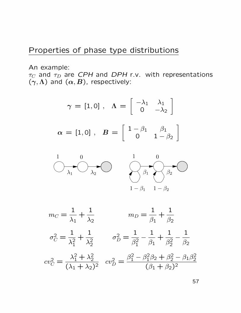
Properties of phase type distributions

An example:τC and τD are CPH and DPH r.v. with representations(γ,Λ) and (α,B), respectively:

γ = [1,0] , Λ =

[−λ1 λ1

0 −λ2

]

α = [1,0] , B =

[1− β1 β1

0 1− β2

]

λ1 λ2

01

β1 β2

01

1− β21− β1

mC =1

λ1+

1

λ2mD =

1

β1+

1

β2

σ2C =

1

λ21

+1

λ22

σ2D =

1

β21

−1

β1+

1

β22

−1

β2

cv2C =

λ21 + λ2

2

(λ1 + λ2)2cv2D =

β21 − β2

1β2 + β22 − β1β2

2

(β1 + β2)2

57

Properties of phase type distributions

Example 1) Fix λ1 and β1 and find λmin2 and βmin2 thatminimizes cv2

C and cv2D :

λmin2 = λ1 ; βmin2 =β1(2 + β1)

2− β1.

→ the minimal cv2C is provided by Erlang(2), but the

minimal cv2D is not discrete Erlang(2).

Example 2) Fix mC and mD, in this case

λ1 =λ2

mCλ2 − 1and β1 =

β2

mDβ2 − 1.

Find λmin2 and βmin2 that minimizes cv2C and cv2

D :

λmin2 =2

mC; βmin2 =

2

mD.

→ both cv2C and cv2

D are Erlang(2) and the minimal co-efficient of variations are:

cv2C =

1

2and cv2

D =1

2−

1

mD.

58

Minimal CV of CPHs

Theorem 1 The squared coefficient of variation of τ ,cv2(τ), satisfies:

cv2(τ) ≥1

N(1)

and the only CPH distribution, which satisfies the equal-ity is the Erlang(N) distribution:

1 0

λλ

0

λ

59

Minimal CV of DPHs

Theorem 2 The squared coefficient of variation of τ ,cv2(τ), satisfies the inequality:

cv2(τ) ≥

〈µ〉(1− 〈µ〉)

µ2if µ < N ,

1

N−

1

µif µ ≥ N .

(2)

where 〈x〉 denotes the fraction part of x.

• for µ ≤ N CVmin provided by the mixture of twodeterministic distributions, e.g.:

00

1 1 1

0〈µ〉

1

1−〈µ〉

• for µ > N CVmin provided by the discrete Erlangdistribution:

1 0

Nµ

Nµ

1− Nµ1− N

µ 1− Nµ

0

Nµ

60

Special PH classes

A unique and minimal representation of the PH class isnot available yet

→ use of simple PH subclasses:

• Acyclic PH distributions

• Hypo-exponential distr. (“series”, “cv < 1”)

• Hyper-exponential distr. (“parallel”, “cv > 1”)

• ...

61

Acyclic PH distributions

The acyclic PH class allows a minimal representationwith only 2N parameters.

Continuous case: A unique minimal representation ofany ACPH distribution is given in one of the three canon-ical forms:

a1 a2 an

λnλ2λ1

1

c1 λ1 λ2 λn−2

c2cn−1

cn

λn−1

1 en

e,n e,n−1 e,2 e,1e,n−2

en−2en−1

The unique representation is based on the elementaryoperation:

λ1

λ2:

1− λ1

λ2

:

λ1

λ2

λ1 λ2

λ1 < λ2

62

Acyclic PH distributions

Discrete case: A unique minimal representation of anyADPH distribution is given in one of the three canonicalforms:

a1 a2 an

pnp2p1

q1 q2 qn

1

c1

qn

p1

q1

p2

q2 qn−1

pn−2

c2cn−1

cn

pn−1

1

qn−1 qn−2

en

e,n e,n−1 e,2 e,1e,n−2

en−2

qn

en−1

q1

The unique representation is based on the elementaryoperation:

p1p2

:

1− p1p2

:

q2

q1

p1

p2

q2q1

p1 p2

p1 < p2

63

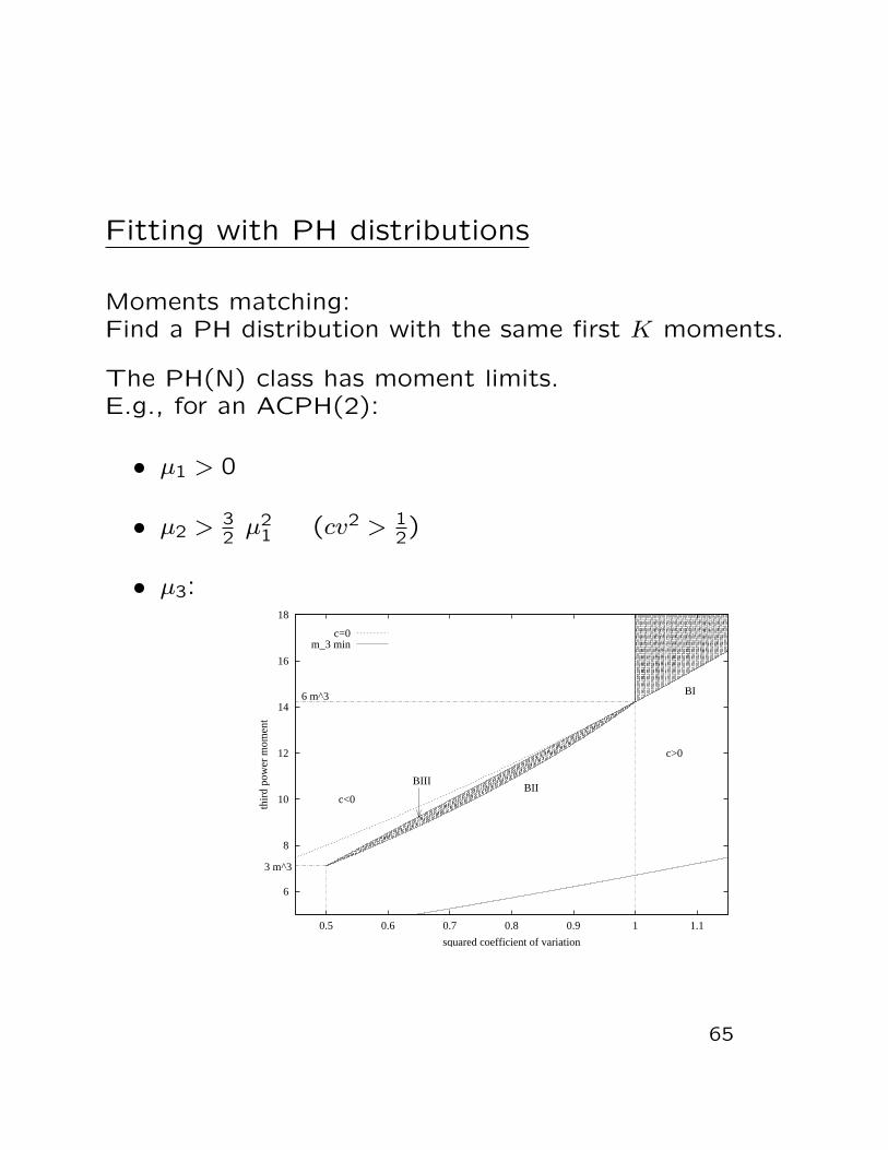
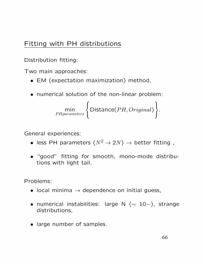
Fitting with PH distributions

Fitting:given a non-negative distribution find a “similar” PHdistribution.

Formally:

minPHparameters

Distance(PH,Original)

,

where Distance is a non-negative valued function.

Measures of similarity:

• a function of a given number of moments(there can be multiple PH distributions with 0 dis-tance)

• a function of the distributions, e.g.,

– squared CDF difference:∫∞

0 (F (t)− F (t))2dt

– density difference:∫∞

0 |f(t)− f(t)|dt

– relative entropy:∫∞

0 f(t) log

(f(t)

f(t)

)dt

There are also heuristic fitting methods, which are hardto formalize.

64

Fitting with PH distributions

Moments matching:Find a PH distribution with the same first K moments.

The PH(N) class has moment limits.E.g., for an ACPH(2):

• µ1 > 0

• µ2 >32µ2

1 (cv2 > 12)

• µ3:

6

8

10

12

14

16

18

0.5 0.6 0.7 0.8 0.9 1 1.1

thir

d po

wer

mom

ent

squared coefficient of variation

c<0

c>0

6 m^3

3 m^3

BI

BIIIBII

c=0m_3 min

65

Fitting with PH distributions

Distribution fitting:

Two main approaches:

• EM (expectation maximization) method,

• numerical solution of the non-linear problem:

minPHparameters

Distance(PH,Original)

.

General experiences:

• less PH parameters (N2 → 2N) → better fitting ,

• “good” fitting for smooth, mono-mode distribu-tions with light tail.

Problems:

• local minima → dependence on initial guess,

• numerical instabilities: large N (∼ 10−), strangedistributions,

• large number of samples.

66

Fitting with PH distributions

00.

51

1.5

22.

53

t

0.2

0.4

0.6

0.8

Den

sity

PH-2

PH-4

PH-8

Ori

g. d

ist.

W1

- W

eibu

ll [1

, 1.5

]

00.

51

1.5

22.

53

t

0.2

0.4

0.6

0.81

1.2

Den

sity

PH-2

PH-4

PH-8

Ori

g. d

ist.

W2

- W

eibu

ll [1

, 0.5

]

00.

20.

40.

60.

81

1.2

t

1234

Den

sity

PH-2

PH-4

PH-8

Ori

g. d

ist.

L1

- L

ogno

rmal

[1,

1.8

]

00.

51

1.5

22.

5t

0.2

0.4

0.6

0.81

Den

sity

PH-2

PH-4

PH-8

Ori

g. d

ist.

L2

- L

ogno

rmal

[1,

0.8

]

00.

51

1.5

22.

5t

0.51

1.52

Den

sity

PH-2

PH-4

PH-8

Ori

g. d

ist.

L3

- L

ogno

rmal

[1,

0.2

]

00.

51

1.5

2t

0.2

0.4

0.6

0.81

1.2

1.4

Den

sity

PH-2

PH-4

PH-8

Ori

g. d

ist.

U1

- U

nifo

rm [

0-1]

00.

51

1.5

22.

53

t

0.2

0.4

0.6

0.81

Den

sity

PH-2

PH-4

PH-8

Ori

g. d

ist.

U2

- U

nifo

rm [

1-2]

00.

51

1.5

22.

53

t

0.1

0.2

0.3

0.4

0.5

0.6

0.7

Den

sity

PH-2

PH-4

PH-8

Ori

g. d

ist.

SE -

Shi

fted

Exp

onen

tial

00.

51

1.5

22.

53

t

0.2

0.4

0.6

0.81

1.2

Den

sity

PH-2

PH-4

PH-8

Ori

g. d

ist.

ME

- M

atri

x E

xpon

entia

l

67

Fitting with PH distributions

Approximating distributions with low coefficient of vari-ation using few phases

−→ fitting with Discrete PH distributions.

Problems of fitting continuous distributions with dis-crete PH:

• discretization method

• discrete time step

68

Fitting with PH distributions

Fitting continuous distributions:

The r.v. X, with cdf FX(x), can be discretized over thediscrete set S = x1, x2, x3, . . . using, e.g.:

xi = i δ

pi = FX

(xi + xi+1

2

)− FX

(xi−1 + xi

2

)This discretization does not preserve the moments ofthe distribution.

A natural requirement of discretization is:

E(Xi) ∼ δi E(Xid), i ≥ 1 ,

where δ is the discrete time step.

If it is fulfilled

E(X) ∼ δE(Xd) and cv(X) ∼ cv(Xd)

→ δ plays significant role in the goodness of fitting.

69

Fitting with PH distributions

DPHs with different discrete time steps versus CPH

0

0.1

0.2

0.3

0.4

0.5

0.6

0.7

0.8

0.9

1

0.4 0.6 0.8 1 1.2 1.4 1.6 1.8

L3 cdf0.1

0.050.025CPH

0

0.5

1

1.5

2

0.2 0.4 0.6 0.8 1 1.2 1.4 1.6 1.8

L3 pdf0.1

0.050.025CPH

70

Applications of Phase type distributions

Non-Markovian models → Markovian analysis

• queueing models (matrix geometric methods)

• performance, performability models

• stochastic Petri net models

Traditionally continuous time models with CPH wereused.

Recently discrete time models gain importance:

• slotted communication protocols

• physical observations at fine time scales

• discrete time stochastic Petri nets

• deterministic or random event time with low vari-ance

• finite support

71

Matrix exponential/geometric distributions

The continuous distribution with density f(t) is matrixexponential if the Laplace transform of f(t) (f∗(s) =∫∞

0− f(t)e−stdt) is a rational function of s.

f∗(s) =a0 + a1s+ a2s2 + . . .+ aNs

N

b0 + b1s+ b2s2 + . . .+ bNsN

The discrete distribution on N with probability massfunction pi = Pr(X = i) (i ∈ N) is matrix geomet-ric if the z transform of the probability mass function(F(z) =

∑∞i=0 z

ipi) is a rational function of z.

F(z) =a0 + a1z + a2z2 + . . .+ aNz

N

b0 + b1z + b2z2 + . . .+ bNzN

The order of a matrix exponential/geometric distribu-tion is the order of the rational function (N).

72

Properties of matrix exp./geom. distributions

Constraints on the coefficients:

f∗(s)|s=0 = F(z)|z=1 = 1

The poles of f∗(s) and F(z) are on the left complex halfplane.

Unfortunately, these properties do not ensure a proba-bility distribution.

The set of matrix exp./geom. distributions of order Nis a rear subset of the order N rational functions.

73

Representation of matrix exp./geom. distr.

Cox’s representation:c 1 c 2 3c

p p 1 p 120

ci: complex transition rates,pi: probability of termination.

“Time domain” representation of matrix exp./geom.distributions:

PDF: f(t) = αeAta

PMF: pk = Pr(X = k) = αBk−1b

Where α, a,b are general real valued vectors and A,Bare general real valued square matrices of order N .

Similar to the transform domain representation, onlyspecial cases of α,A, a and α,B,b result proper PDFsand PMFs.

74

Renewal process

Renewal process:

Point/Counting process with i.i.d. inter-event time

0 1 2 3 4

1 2 3 4 5

2 3

T T T T T t

N(t)

τ τ τ τ τ

N(t)=2 <=> T < t < T

Point process: τ1, τ2, τ3, . . .

Counting process: N(t)

Parameters:

• renewal function: M(t) = E(N(t))

• index of dispersion of count: IDC(t) =σ(N(t))

E(N(t))

75

Equilibrium distribution

Paradox of random arrival in Poisson process.

n n+1 n+2 n+3 n+4

n+1 n+3n−1 n n+2 n+4

Random arrival

Time to the next arrival

t

τ τ τ τ τ

T T TT T T

Paradox:

• τn (n = 1,2, . . .) is exponentially (λ) distributed,

• due to the memoryless property the time to thenext arrival is exponentially (λ) distributed as well.

Is τ3 longer or the remaining time is shorter than expo-nential (λ)???

76

Equilibrium distribution

Basic properties:

• the random arrival instance falls in longer intervalswith higher probability,

• inside the selected interval the random arrival in-stance is uniformly distributed.

Distribution of the length of the selected interval (SI):

fSI(t) =tf(t)∫

xxf(x)dx

=tf(t)

E(τ)

Distribution of time to next arrival (T ) when the lengthof the interval is x:

fT |x(t) =

1/x if 0 < t < x0 otherwise

77

Equilibrium distribution

Equilibrium distribution:

fT(t) =

∫ ∞x=0

fT |x(t) fSI(x) dx =

∫ ∞x=t

1/xxf(x)

E(τ)dx

fT(t) =1− F (t)

E(τ),

f∗T(s) =1/s− F ∗(s)

E(τ)=

1− sF ∗(s)s E(τ)

=1− f∗(s)s E(τ)

,

Moments of equilibrium distribution:

E(T n) =

∫ttn(1− F (t))dt

E(τ)=

E(τn+1)

(n+ 1)E(τ)

78

Renewal function

Distribution of Ti:

Pr(Ti < t) = F (t)⊗ F (t)⊗ . . .⊗ F (t)︸ ︷︷ ︸i

= F (i)(t)

Renewal function and inter-arrival time distribution:

M(t) = E(N(t)) =∞∑i=0

i Pr(N(t) = i) =

∞∑i=0

i Pr(Ti < t < Ti+1) =∞∑i=0

i

(Pr(Ti < t)− Pr(Ti+1 < t)

)∞∑i=0

i

(F (i)(t)− F (i+1)(t)

)=

∞∑i=0

i F (i)(t)−∞∑i=1

(i− 1) F (i)(t)

−→ M(t) =∞∑i=1

F (i)(t)

79

Renewal equation

Relation of renewal function and inter-arrival time dis-tribution:

M(t) = E(N(t)) = F (t) +∞∑i=1

F (i+1)(t) =

F (t) +∞∑i=1

∫ t

u=0F (i)(t− u) dF (u) =

F (t) +

∫ t

u=0

∞∑i=1

F (i)(t− u) dF (u)

−→ M(t) = F (t) +

∫ t

u=0M(t− u) dF (u)

Renewal equation for densities: (m(t) =d

dtM(t))

−→ m(t) = f(t) +

∫ t

u=0m(t− u) f(u) du

Renewal equation in transform domain:

M∼(s) =F∼(s)

1− F∼(s), F∼(s) =

M∼(s)

1 +M∼(s)

80

Initial condition of a renewal process

Depending on the origin of the time access:

• Ordinary renewal process:

Time starts at renewal → the distribution of τ1 isthe same.

• Delayed renewal process:

Time starts between renewals → the distribution ofτ1 is different

M∼(s) =F∼1 (s)

1− F∼(s)

• Stationary renewal process:

(special case) the distribution of τ1 is the equilib-rium distribution

M∼(s) =F∼1 (s)

1− F∼(s)=

1−F ∼(s)s E(T )

1− F∼(s)=

1

s E(T )

−→ M(t) =t

E(T ), m(t) =

1

E(T )

81

Behaviour of the renewal function

Taylor expansion of F∼(s):

F∼(s) =∞∑i=0

si

i!

di

dsiF∼(s)

∣∣∣∣∣s=0

=∞∑i=0

(−1)isi

i!E(T i)

Series expansion of M∼(s):

M∼(s) =F∼(s)

1− F∼(s)=

1

s2 E(T )+E(T 2)− 2E2(T )

s 2E2(T )+σ (1/s)

Series expansion of the renewal function:

M(t) =t

E(T )+E(T 2)− 2E2(T )

2E2(T )+ σ (1)

0.5 1 1.5 2t

0.2

0.4

0.6

0.8

1

1.2

renewal

82

Phase type renewal process

Inter-arrival time is PH distributed.

N(t): number of renewalsJ(t): phase of the PH distribution

Logic behaviour:

α

i

i

a

i i i

A A A

j j ja

α

i

i

a

α

i

i

α α

a a a

α

jj

j

j

j j

Tangible behaviour:

i iαai α j

ja α jja iα

ai iαai α j

ja α jja iα

ai iαai α j

ja α jja iα

ai

A

j

i

A

j

i

A

j

−→ N(t), J(t) is a Markov chain.

83

Phase type renewal process

Structure of the generator matrix:

Q =

A aα

A aα

A aα

A aα

. . .

On the block level it is similar to the structure of aPoisson process.

−→ “quasi” birth process.

84

Phase type renewal process

Phase process (J(t)) is a CTMC:

Logic behaviour:

j

αi

α j

ia

Aij

a

i

A

j

Tangible behaviour:

ij ia α jA i

A

j

+

Generator matrix: QJ = A + aα

Properties:

• for i 6= j: QJij = Aij + aiαj ≥ 0,

• QJ1I = A1I + a α1I︸︷︷︸1

= A1I + a = 0

85

Phase type renewal process

M(t) = E(N(t)), m(t) =d

dtM(t)

Short time behaviour:

N(t+ ∆)−N(t)|J(t) = i =

0 1− ai∆ + σ(∆)1 ai∆ + σ(∆)> 1 σ(∆)

−→E(N(t+ ∆)−N(t)|J(t) = i) =

M(t+ ∆)−M(t)|J(t) = i = ai∆ + σ(∆)

−→m(t)|J(t) = i = ai

−→m(t) =

∑i∈S

Pr(J(t) = i) ai =∑j∈S

∑i∈S

αjPr(J(t) = i|J(0) = j) ai =∑j∈S

∑i∈S

αj[eQJt

]jiai = α eQJt a

86

Phase type renewal process

The time to the next arrival at an arbitrary time t is PHdistributed with parameters (p(t),A),

where p(t) is the transient distribution of the phase pro-cess (pi(t) = Pr(J(t) = i))

Initial condition of a PH renewal process:

• Ordinary PH renewal process:

p(0) = α,

• Delayed PH renewal process:

p(0) is an arbitrary distribution,

• Stationary PH renewal process:

p(0) = π,

where π is the stationary distribution of the phaseprocess. (0 = πQJ,π1I = 1)

87

Phase type renewal process

Sojourn time in state j in a renewal interval startingfrom state i: Tij.

Mean sojourn time:

E(Tij) =δij

−Aii+∑k,k 6=i

Aik

−AiiE(Tkj)

0 = δij +∑k

AikE(Tkj) −→ 0 = I + AT

T = (−A)−1 −→ E(Tij) = [(−A)−1]ij

88

Phase type renewal process

Sojourn time distribution, i = j:

t∗ii(s) =−Aiis−Aii

ai

−Aii+∑k,k 6=i

Aik

−Aiit∗ki(s)

s t∗ii(s) = ai +

∑k

Aikt∗ki(s)

i 6= j:

t∗ij(s) =ai

−Aii+∑k,k 6=i

Aik

−Aiit∗kj(s)

0 = ai +∑k

Aikt∗kj(s)

in general:

δij s t∗ij(s) = ai +

∑k

Aikt∗kj(s)

s Diag〈t∗ii(s)〉 = ae + A t∗(s),

where e = 1,1, . . . ,1.

89

Phase type renewal process

Mean time spent in j in a renewal interval:

τj =∑i

αiE(Tij) −→ τ = α(−A)−1

Portion of time spent in j in a renewal interval:

νj =τj∑k τk

=

∑i αiE(Tij)∑

k

∑i αiE(Tik)

−→ ν =α(−A)−1

α(−A)−11I

Theorem: ν = π (time average = stationary behaviour)

Proof: ν1I = 1 by definition, and

νQj = ν(A + aα) =α(−A)−1 (A−A1Iα)

α(−A)−11I

=−α+α1Iα

α(−A)−11I=−α+α

α(−A)−11I= 0

90

Phase type renewal process

If Q is a generator of an irreducible CTMC then Q issingular (@Q−1), since 0 is an eigenvalue of Q (0 = πQ).

Theorem: (Q− 1Iπ) is non-singular.

(I.e. (Q− 1Iπ)−1 exists.)

Proof: Assume x 6= 0 and x(Q− 1Iπ) = 0,

then x(Q− 1Iπ)1I = 01I −→ x1I = 0;

but from x(Q− 1Iπ) = 0 we also have xQ = x1I︸︷︷︸0

π = 0,

it is possible only when x is proportional to π, but it isin contrast with x1I = 0.

91

Phase type renewal process

Analysis of the renewal function, M(t) = E(N(t)) :

M(t) =

∫ t

x=0m(x) dx = α

∫ t

x=0eQJx dx a =

α

∫ t

x=0

∞∑i=0

xi

i!QJ

i dx a = α∞∑i=0

ti+1

(i+ 1)!QJ

i a =

α∞∑i=0

ti+1

(i+ 1)!QJ

i(QJ − 1Iπ)(QJ − 1Iπ)−1 a =

α∞∑i=0

ti+1

(i+ 1)!QJ

i+1(QJ − 1Iπ)−1 a

−α∞∑i=0

ti+1

(i+ 1)!QJ

i1I︸ ︷︷ ︸0 if i>0

π(QJ − 1Iπ)−1 a =

α(eQJt − I)(QJ − 1Iπ)−1 a− t α1I︸︷︷︸1

π(QJ − 1Iπ)−1︸ ︷︷ ︸−π

a =

α(eQJt − I)(QJ − 1Iπ)−1 a + t π a

since

π = π1I︸︷︷︸1

π − πQJ︸︷︷︸0

= π(1Iπ −QJ)

92

Phase type renewal process

Examples:

hyper-exponential: α = 0.5,0.5, A =−0.1 0

0 −10

1 2 3 4 5t

0.2

0.4

0.6

0.8

1

lambda

0.5 1 1.5 2t

0.2

0.4

0.6

0.8

1

1.2

renewal

93

Phase type renewal process

Examples:

hypo-exponential: α = 1,0, A =−0.5 0.5

0 −0.5

1 2 3 4 5t

0.2

0.4

0.6

0.8

1

lambda

0.5 1 1.5 2t

0.1

0.2

0.3

0.4

0.5

renewal

94

Phase type renewal process

Distribution of the number of renewals(short term behaviour)

Pj(n, t) = Pr(N(t) = n, J(t) = j),

P(n, t) = Pj(n, t) (vector)

The transient behaviour of the (N(t), J(t)) CTMC isdP(t)

dt= P(t)Q, where P(t) = P(0, t), P(1, t), . . ..

For P(0, t) and P(i, t) (i > 0) we have:

dP(0, t)

dt= P(0, t)A

dP(i, t)

dt= P(i, t)A + P(i− 1, t)aα

with initial conditions: P(0,0) = α, P(i,0) = 0.

z-transform:

dP(z, t)

dt= P(z, t)A + zP(z, t)aα = P(z, t)(A + zaα)

with initial condition: P(z,0) = α.

Solution: P(z, t) = α e(A+zaα)t

95

Phase type renewal process

Distribution of the number of renewals(renewal theory)

Pij(n, t) = Pr(N(t) = n, J(t) = j|J(0) = i)

P(n, t) = Pij(n, t) (matrix)

no renewal in (0, t): P(0, t) = eAt

renewal in (0, t) (at time t− u):

P(k, t) =

∫ t

u=0eA(t−u)aαP(k − 1, u)du

z-transform:

P(z, t) = eAt + z

∫ t

u=0eA(t−u)aαP(z, u)du

Solution can be obtained by multiplying with eAt andcalculating derivatives.

96

Markov arrival process

A point process characterized by

• N(t): number of arrivals

• J(t): phase of the PH distribution

Restriction in PH renewal process:

the phase distribution is reset at arrivals.

MAP:

the phase distribution after an arrival is arbitrary.

Process behaviour:

i

j

D1

D1

D1D1

ii

ij

jijj

i

j

D1

D1

D1D1

ii

ij

jijj

i

j

D1

D1

D1D1

ii

ij

jijj

D0 D0 D0

−→ N(t), J(t) is still a Markov chain.

97

Markov arrival process

Common notation:

• D0 = A – phase transitions without arrival

• D1 – phase transitions with one arrival

Structure of the generator matrix:

Q =

D0 D1

D0 D1

D0 D1

D0 D1

. . .

On the block level it is similar to the structure of aPoisson process.

−→ “quasi” birth process.

98

Properties of Markov arrival process

• the phase distribution at arrival instances form aDTMC with P = (−D0)−1D1

−→ correlated initial phase distributions,

• inter-arrival time is PH distributed with representa-tion (α0,D0), (α1,D0), (α2,D0), . . .−→ correlated inter-arrival times,

• phase process (J(t)) is a CTMC with generatorD = D0 + D1

D1ijD0 ij

i

j

+

99

Properties of Markov arrival process

• (time) stationary phase distribution α is the solutionof αD = 0, α1I = 1.

• (embedded) stationary phase distribution after anarrival π is the solution of πP = π, π1I = 1.

• stationary inter arrival time (X) is PH distributedwith representation (π,D0), whose nth moment isE(Xn) = n!π(−D0)−n1I .

• the initial and consecutive state dependent densityof the inter arrival time is [fij(t)] = eD0tD1.

• the stationary arrival intensity is

λ = αD11I =1

E(X)=

1

π(−D0)−11I.

• similar to PH renewal processes

α =π(−D0)−1

π(−D0)−11I=π(−D0)−1

E(X)= λπ(−D0)−1.

100

Properties of Markov arrival process

The joint pdf of X0 and Xk is

fX0,Xk(x, y) = πeD0xD1P

k−1eD0yD11I.

Due to the Markovian behaviour of MAPs X0 and Xk

depend only via their initial states !!!!

101

Properties of Markov arrival process

Lag k correlation:

E(X0Xk) =

∫ ∞t=0

∫ ∞τ=0

t τ πeD0tD1Pk−1eD0τD11I dτ dt

= π(−D0)−2D1Pk−1(−D0)−2 D11I︸︷︷︸−D01I

= π(−D0)−1Pk(−D0)−11I =1

λαPk(−D0)−11I

Since∫ ∞t=0

t eD0tdt =[t (D0)−1eD0t

]∞0︸ ︷︷ ︸

0

−∫ ∞t=0

(D0)−1 eD0tdt

and∫ ∞t=0

eD0tdt = limT→∞

∞∑i=0

D0i

i!

∫ T

0tidt = lim

T→∞

∞∑i=0

D0i

i!

T i+1

i+ 1

= limT→∞

(D0)−1

(eD0T︸︷︷︸→0

−I)

= (−D0)−1

102

Properties of Markov arrival process

Covariance:

Cov(X0, Xk) = E(X0Xk)− E2(X) =

=1

λαPk(−D0)−11I−

1

λ2

Coefficient of correlation:

Corr(X0, Xk) =Cov(X0, Xk)

E(X2)− E2(X)=

E(X0Xk)E2(X)

− 1

E(X2)E2(X)

− 1

=λ αPk(−D0)−11I− 1

2λ α(−D0)−11I− 1

103

Properties of Markov arrival process

In general, for a0 = 0 < a1 < a2 < . . . < ak,

the joint density is:

fXa0,Xa1,...,Xak(x0, x1, . . . , xk) =

= πeD0x0D1Pa1−a0−1eD0x1D1Pa2−a1−1 . . . eD0xkD11I ,

and the joint moment is:

E(Xi0a0, Xi0

a1, . . . , Xi0

ak) =

= πi0!(−D0)−i0Pa1−a0i1!(−D0)−i1Pa2−a1 . . . ik!(−D0)−ik1I .

104

Batch Markov arrival process

MAP with batch arrivals.

Process behaviour:

ii

D2jj

D3jj

D2jj

D2ii

D2ij D2ij

D2ii

D1 D1

D1

D1D1

ii

ij

jijj

D0i

j

D1

D1D1

ij

jijj

i

j

D1

D1

D1D1

ii

ij

jijj

i

j

D0 D0

−→ N(t), J(t) is still a Markov chain.

105

Batch Markov arrival process

Common notation:

• D0 – phase transitions without arrival

• Dk – phase transitions with k arrivals

Structure of the generator matrix:

Q =

D0 D1 D2 D3 D4

D0 D1 D2 D3

D0 D1 D2

D0 D1

. . .

Properties of matrices Dk:

• D0: D0ij ≥ 0 for i 6= j, and D0ii ≤ 0

• for k ≥ 1: Dkij ≥ 0

•∞∑k=0

Dk1I = 0 (row-sum=0)

106

Batch Markov arrival process

Properties of batch Markov arrival process:

• the phase distribution at arrival instances form aDTMC−→ correlated initial phase distributions,

• inter-arrival time is PH distributed with representa-tion (α0,D0), (α1,D0), (α2,D0), . . .−→ correlated inter-arrival times,

• batch arrivals,

• phase process (J(t)) is a CTMC with generatorD =

∑∞k=0 Dk

D1ijD0 ijD2+ +iji

j

107

Batch Markov arrival process

Examples:

• bath PH renewal process:D0 = A, Dk = pkaα.

• MMPP (Markov modulated Poisson process):D0 = Q− diag<λ>, D1 = diag<λ>.

• IPP (Interrupted Poisson process):

D0 =−α−λ α

0 −β , D1 =λ 00 0

.

• batch MMPP :D0 = Q− diag<λ>, Dk = pk diag<λ>.

108

Batch Markov arrival process

Examples:

• filtered MAP (arrivals discarded with probability p):D0 = D0 + pD1, D1 = (1− p)D1.

• cyclicly filtered MAP (every second arrivals are dis-carded with probability p):

D0 =D0 0

pD1 D0, D1 =

0 D1

(1−p)D1 0.

• superposition of BMAPs:Dk = Dk

⊕Dk,

Kronecker product: A⊗

B =A11B . . . A1nB

... ...An1B . . . AnnB

Kronecker sum: A⊕

B = A⊗

IB + IA

⊗B

109

Batch Markov arrival process

• Departure process of an M/M/1/2 queue:

D0 =−λ λ

−λ−µ λ−µ

D1 = µµ

• Departure process of an MAP/M/1/1 queue:

D0 =D0 D1

0 D0 + D1 − µI, D1 =

0 0µI 0

.

• Correlated inter-arrivals (λ1 6= λ2):

D0 =−λ1 0

0 −λ2D1 =

pλ1 (1− p)λ1

(1− p)λ2 pλ2

p ∼ 1→ positive correlated consecutive inter-arrivals

p ∼ 0→ negative correlated consecutive inter-arrivals

110

Batch Markov arrival process

Regular BMAPs:

• phase-process (D) is irreducible,

• mean inter-arrival time is positive and finite – D0

non-singular,

• mean arrival rate, d =∑∞

k=0 kDk1I, is finite.

Properties of regular BMAPs:

• M(t) = E(N(t)) mean number of arrivals,

m(t) = ddtM(t) arrival rate,

• π stationary phase distribution at arrival,

• α stationary phase distribution (αD = 0,α1I = 1)

m(t) = πeDtd, λ = limt→∞

m(t) = αd,

M(t) =

∫ t

x=0m(x)dx = αd t+ π(eDt − I)(D− 1Iα)−1d

111

Batch Markov arrival process

Distribution of the number of arrivals(short term behaviour):

Pij(n, t) = Pr(N(t) = n, J(t) = j|N(0) = 0, J(0) = i)

P(n, t) = Pij(n, t) (matrix)

The transient behaviour:

d

dtP(n, t) =

n∑k=0

P(n− k, t)Dk

initial conditions:

P(0,0) = I, and P(n,0) = 0 for n > 0.

z transform: P(z, t) =∞∑n=0

znP(n, t).

d

dtP(z, t) =

∞∑n=0

znn∑

k=0

P(n− k, t)Dk

=∞∑k=0

zk∞∑n=k

zn−kP(n− k, t)Dk = P(z, t)D(z)

Solution: P(z, t) = eD(z)t, since P(z,0) = I

112

Batch Markov arrival process

Distribution of the number of arrivals(regenerative approach):

P(0, t) = eD0t,

P(n, t) =

∫ t

τ=0eD0τ

n∑k=1

Dk P(n−k, t−τ)dτ, n ≥ 1

Laplace transform: P∗(n, s) =

∫ ∞t=0

e−stP(n, t)dt.

P∗(0, s) = (sI−D0)−1,

P∗(n, s) = (sI−D0)−1n∑

k=1

Dk P∗(n−k, s), n ≥ 1

z transform: P∗(z, s) =∞∑n=0

znP∗(n, s).

P∗(z, s) = (sI−D0)−1(I + (D(z)−D0)P∗(z, s)),

P∗(z, s) = (sI−D(z))−1,

Inverse Laplace transform:

P(z, t) = eD(z)t.

113

Quasi birth-death process

Continuous time QBD:

N(t), J(t) is a CTMC, where

• N(t) is the “level” process (e.g., number of cus-tomers in a queue),

• J(t) is the “phase” process (e.g., state of the en-vironment).

N(t), J(t) is a Quasi birth-death process if transitionsare restricted to one level up or down or inside the samelevel.

Bii

FijBkk

FjiFjj

L ij Bkk

Fij

Bii

FjiFjj

L ij

Fjj

Fji

Bkk

Fij

Bii

ijL’

i

j

i

j

i

j

L L

k kk

L’

Level 0 is irregular (e.g., no departure).

114

Quasi birth-death process

Applied notation:

• F – (forward) transitions one level up (e.g., arrival)

• L – (local) transitions in the same level

• B – (backward) transitions one level down (e.g.,departure)

• L′ – irregular block at level 0.

(In the L-R book: F = A0, L = A1, B = A2.)

Structure of the generator matrix:

Q =

L′ F

B L F

B L F

B L F

. . . . . .

On the block level it has a birth-death structure.

−→ “quasi” birth-death process.

115

Quasi birth-death process

Example: PH/M/1 queue

• arrival process: PH renewal process with represen-tation τ,T, (t = −T1I)

• service time: exponentially distributed with param-eter µ.

Structure of the transition probability matrix:

Q =

T tτ

µI T−µI tτ

µI T−µI tτ

µI T−µI tτ

. . . . . .

That is F = tτ , L = T− µI, B = µI and L′ = T.

116

Quasi birth-death process

Example: MAP/PH/1/K queue

• arrival process: MAP D0,D1,

• service time: PH(τ,T), (t = −T1I).

Structure of the transition probability matrix:

Q =

L′ F′

B′ L . . .

B . . . F

. . . L F

B L”

Where

F = D1⊗

I, L = D0⊕

T, B = I⊗tτ ,

F′ = D1⊗τ , L′ = D0, B′ = I

⊗T and

L” = (D0 + D1)⊕

T.

117

Condition of stability

Phase process in the regular part (n > 1) is a CTMCwith generator matrix:

A = F + L + B

Assuming A is irreducible, the stationary solution of Ais:

αA = 0,α1I = 1

The stationary drift of the level process is:

d = αF1I−αB1I

Condition of stability:

d = αF1I−αB1I < 0

118

Matrix geometric distribution

Stationary solution: πQ = 0, π1I = 1.

Partitioning π: π = π0,π1,π2, . . .

Decomposed stationary equations:

π0L′ + π1B = 0

πn−1F + πnL + πn+1B = 0 ∀n ≥ 1

∞∑n=0

πn1I = 1

Conjecture: πn = πn−1R → πn = π0Rn

This conjecture gives:

π0L′ + π0RB = 0

π0Rn−1F + π0RnL + π0Rn+1B = 0 ∀n ≥ 1

∞∑n=0

π0Rn1I = π0(I−R)−11I = 1

119

Matrix geometric distribution

The solution is defined by vector π0 and matrix R:

Matrix R is the solution of the matrix equation:

F + RL + R2B = 0

Vector π0 is the solution of linear system:

π0(L′ + RB) = 0

π0(I−R)−11I = 1

Note that L′+ RB (= L′+ FG) is the generator matrixof the restricted process on level 0.

120

Matrix geometric distribution

Properties of R:

• the matrix equation has more than one solutions.

• if the QBD is stable there is a solution R whoseeigenvalues (λi(R)) are |λi(R)| < 1 and this is therelevant R matrix.

• (if the QBD is not stable there is a solution R whoseeigenvalues (λi(R)) are |λi(R)| ≤ 1 and this is therelevant R matrix.)

Stochastic interpretation:

Rij is the ratio of the mean time spent in (n, j) and themean time spent in (n−1, i) before the first return tolevel n−1 starting from (n−1, i).

In a homogeneous QBD Rij is independent of n.

121

Analysis of the level process

Example: busy period of the M/M/1 queue

The busy period of the M/M/1 queue starts when acustomer arrives to an idle system, and it ends whenthe system becomes idle again, i.e., “the level processmoves from 1 to 0”

Let T be the time of the busy period and g(s) = E(e−sT)its Laplace transform.

g(s) =µ

λ+ µ

λ+ µ

λ+ µ+ s+

λ

λ+ µ

(λ+ µ

λ+ µ+ sg2(s)

)At the beginning of the busy period the process staysexp. (λ+µ) time at level 1. After that it moves to level

0 with probabilityµ

λ+ µand to level 2 with probability

λ

λ+ µ.

From level 2, it returns to level 0 in two steps: fromlevel 2 to 1 and from level 1 to 0.

Due to the homogeneous structure of the chain thesetwo times are i.i.d.

122

Analysis of the level process

γn denotes the time of the first visit to level n:

γn = min(t|t > 0, N(t) = n)

First visit from level n to n− 1:

Gij(t) = Pr(J(γn−1) = j, γn−1 < t|N(0) = n, J(0) = i)

gij(t) =d

dtGij(t), G∼ij(s) =

∫ ∞t=0

e−stgij(t)dt.

Transition from level n to n− 1:

• direct step down,

• transition inside level n,

• transition to level n+ 1:

G∼ij(s) =−Lii

s− Lii

Bij

−Lii+

∑k∈S,k 6=i

Lik−Lii

G∼kj(s)

+∑k∈S

Fik

−Lii

∑`∈S

G∼k`(s)G∼`j(s)

),

that is

0 = B + (L− sI) G∼(s) + FG∼2(s).

123

Analysis of the level process

First state visited in level n− 1 starting from level n:

Gij = Pr(J(γn−1) = j|N(0) = n, J(0) = i)

Gij = limt→∞

Gij(t) ⇒ Gij = lims→0

G∼ij(s) ⇒

0 = B + LG + FG2

124

Restricted process

The state space of the irreducible CTMC with generatorQ is divided into disjoint subset U and D.

The decomposed generator matrix is

Q =Q1 Q2

Q3 Q4.

Restricted process:

We study the process during its visits to U. I.e. the clockis stopped when the CTMC visits D and is resumed whenit returns to U.

The obtained restricted process is a CTMC with gener-ator

QU = Q1 + Q2PD→U

where for i ∈ D and j ∈ U

[PD→U]ij = Pr(X(γU) = j | X(0) = i)

and γU is the fist time when the process visits U.

From PD→U = (−Q4)−1Q3 we have

QU = Q1 + Q2(−Q4)−1Q3

The restricted process is also referred to as stochastic

complement.

125

Analysis of the level process

Time spent at level n before visiting level n− 1:

We consider N(t), J(t) which starts at level n (N(0) =n) and terminates when N(t) = n− 1.

Restricted process on level n:time (clock) increases as long as N(t) = n and it stopswhen N(t) > n.

The restricted process is a CTMC with generator

U = L + FG.

The mean time spent in level n is characterized by(−U)−1, hence

U = L + F(−U)−1B

where L stands for the transitions inside level n andF(−U)−1B describes the effect of transitions to leveln+ 1 and the first return to level n.

126

Analysis of the level process

E(Tij) – mean time spent in state n + 1, j before thefirst jump to level n starting from n, i .

Tij is 0, if a transition to level n − 1 or to level n takesplace, hence

E(Tij) =∑k

Fik

−Lii(−U)−1

kj

Mean time spent in state n, i is1

−Lii.

The ratio of time spent in n+ 1, j and in n, i beforea jump to level n is

Rij =

∑k

Fik

−Lii(−U)−1

kj

1

−Lii

=∑k

Fik (−U)−1kj .

That is

R = F (−U)−1.

127

Matrix geometric distribution

Summary:Matrices describing a QBD:

Matrix R:“Ratio of time spent at level n and level n + 1 beforethe first return to level n”

F + RL + R2B = 0

Matrix G:“The first state visited at level n−1 starting from n”

Gij = Pr(J(γn−1) = j|N0 = n, J0 = i)

FG2 + LG + B = 0

Matrix U:“Generator of the QBD process restricted to level nbefore returning to n− 1”

→ (−U)−1 “mean time spent at level n beforevisiting level n− 1”

U = L + F(−U)−1B

128

Matrix geometric distribution

Relation of matrices describing a QBD:

U = L + FG

= L + RB

G = (−U)−1B

= (−L−RB)−1B

R = F(−U)−1

= F(−L− FG)−1

129

Matrix geometric distribution

Properties of R, U and G in a stable QBD:

• R: “ratio of mean time spent in level n+ 1 and n”(0 ≤ Rij).

The eigenvalues (λi(R)) are |λi(R)| < 1.

• U: is an incomplete generator matrix (for i 6= j,0 ≤ Uij, 0 ≥ Uii, U1I ≤ 0).

• G: is a stochastic matrix (0 ≤ Gij ≤ 1, G1I = 1I).

The properties of G are easier to check and

R = F (−L− FG)−1

130

Transient measure for U

Sojourn probability in level n before moving to level n− 1:

Vij(t) = Pr(N(t) = n, J(t) = j, γn−1 > t|N(0) = n, J(0) = i)

Vij(t|H = h) =

δij h > t∑k 6=i

Lik

−LiiVkj(t− h)+

+∑k

∑`

∫ t−h

τ=0

Fik

−Liigk`(τ)V`j(t− h− τ)dτ h < t

where gij(t) = ddtGij(t). Applying the law of total prob-

ability, Vij(t) =∫∞h=0−Liie

LiihVij(t|H = h)dh, gives

Vij(t) =

∫ ∞h=t

−LiieLiihδijdh

+

∫ t

h=0−LiieLiih

(∑k 6=i

Lik

−LiiVkj(t− h)+

+∑k

∑`

∫ t−h

τ=0

Fik

−Liigk`(τ)V`j(t− h− τ)dτ

)dh.

131

Relation of V?(s), U and G∼(s)

Its Laplace transform, V ?ij(s) =

∫∞t=0 e

−stVij(t)dt, gives

V?(s) =

sI− L− F G∼(s)︸ ︷︷ ︸g?(s)

−1

.

The mean time spent in (n, j) is∫ ∞t=0

Vij(t)dt = lims→0

V ?ij(s) = (−L− FG)−1

ij = (−U)−1ij .

By definition

gij(t) =∑k

Vik(t)Bkj,

and consequently

g?(s) = G∼(s) = V?(s)B.

132

Transient measure for R

Sojourn probability in level n+ 1 before returning to level n:

Rij(t) = lim∆→0

1

∆Pr

(N(t) = n+ 1, J(t) = j, γn > t,

transition in (−∆,0)

| N(−∆) = n, J(−∆) = i

)=

=∑k

FikVkj(t).

From which R?ij(s) =

∫∞t=0 e

−stRij(t)dt is

R?(s) = FV?(s)

and the mean time spent in (n+ 1, j) is∫ ∞t=0

Rij(t)dt = lims→0

R?ij(s) = Rij.

133

Summary of transient measures

From

FV?(s)B = R?(s)B = FG∼(s),

we have

V?(s) = (sI− L− FV?(s)B)−1 ,

sR?(s) = F + R?(s)L + R?2(s)B,

and the quadratic equation for G∼(s) on page 123.

134

Algorithms to compute R/G

• Linear

• Quadratic

– Logarithmic reduction

– Newton’s iteration

– Cyclic reduction

135

Linear algorithms

Linear progression algorithm to calculate G:

G := 0;REPEAT

G := (−L− FG)−1 B;UNTIL||1I−G1I|| ≤ ε

Linear boundary algorithm to calculate G:

G := I;REPEAT

Gold := G;G := (−L− FG)−1 B;

UNTIL||G−Gold|| ≤ ε

Linear algorithm to calculate R:

R := 0;REPEAT

Rold := R;R := F (−L−RB)−1 ;

UNTIL||R−Rold|| ≤ ε

136

Linear algorithms

Stochastic interpretation of the linear progression algo-rithm after i iterations:

G0 = 0,G1 = (−L)−1B,G2 = (−L− F(−L)−1B)−1B,G3 = . . .

where

Q1 =B L

, Q2 = B L F

B L

, Q3 = . . .

[Gn]ij = Pr(J(γ0) = j, γ0 < γn+1|N0 = 1, J0 = i)

Bii

FijBkk

FjiFjj

L ij

Fij

Fjj

L ijBkk

Bii

Fji

i

j

i

j

i

j

L L

k kk

137

Linear algorithms

Stochastic interpretation of the linear boundary algo-rithm after i iterations:

G0 = I,G1 = (−L− F)−1B,G2 = (−L− F(−L− F)−1B)−1B,G3 = . . .

where

Q1 =B L+F

, Q2 = B L F

B L+F

, Q3 = . . .

Bii

FijBkk

FjiFjj

L ij

FijL ijBkk

Bii

Fji

Fjj

i

j

i

j

i

j

L L

k kk

138

Discrete time Quasi birth-death process (DTQBD)

N(t), J(t) is a DTMC, where

• N(t) is the “level” process (e.g., number of cus-tomers in a queue),

• J(t) is the “phase” process (e.g., state of the en-vironment).

Structure of the transition probability matrix:

P =

L′ F

B L F

B L F

B L F

. . . . . .

B + L + F is a stochastic matrix,

L′ + F as well.

139

Condition of stability (DTQBD)

Phase process in the regular part (n > 1) is a DTMCwith generator matrix:

PJ = F + L + B

Assuming PJ is irreducible, the stationary solution of PJ

is the solution of:

αPJ = α,α1I = 1

The stationary drift of the level process is:

d = αF1I−αB1I

Condition of stability:

d = αF1I−αB1I < 0

140

Matrix geometric distribution (DTQBD)

Stationary solution: πP = π, π1I = 1.

Partitioning π: π = π0,π1,π2, . . .

Decomposed stationary equations:

π0L′ + π1B = π0

πn−1F + πnL + πn+1B = πn ∀n ≥ 1

∞∑n=0

πn1I = 1

The solution is πn = π0Rn, where

Matrix R is the solution of the matrix equation

F + RL + R2B = R

that is

F + R(L− I) + R2B = 0

Vector π0 is the solution of linear system:

π0(L′ + RB) = π0

π0(I−R)−11I = 1

( L′+ RB = L′+ FG is the transition probability matrixof the restricted process on level 0.)

141

Analysis of the level process (DTQBD)

First state visited in level n− 1

starting from level n:

Gij = Pr(J(γn−1) = j, γn−1 <∞|N(0) = n, J(0) = i)

From the stochastic interpretation

Gij = Bij +∑k

LikGkj +∑k

∑`

FikGk`G`j

from which

0 = B + (L− I)G + FG2

142

Restricted process (DTQBD)

The state space of the irreducible DTMC with transitionprobability matrix P is divided into disjoint subset U andD.

The decomposed generator matrix is

P =P1 P2

P3 P4.

Restricted process:

We study the process during its visits to U. I.e. the clockis stopped when the DTMC visits D and is resumed whenit returns to U.

The obtained restricted process is a DTMC with tran-sition probability matrix

PU = P1 + P2PD→U

where for i ∈ D and j ∈ U

[PD→U]ij = Pr(X(γU) = j | X(0) = i)

and γU is the fist time when the process visits U.

143

Restricted process (DTQBD)

The mean time spent in the states of D during a visitto D is

∑i P4

i = (I−P4)−1.

From PD→U = (I−P4)−1P3 we have

PU = P1 + P2(I−P4)−1P3

144

Analysis of the level process (DTQBD)

Time spent at level n before visiting level n− 1:

We consider N(t), J(t) which starts at level n (N(0) =n) and terminates when N(t) = n− 1.

Restricted process on level n:time (clock) increases as long as N(t) = n and it stopswhen N(t) > n.

The restricted process is a DTMC with generator

U = L + FG.

The mean time spent in level n is characterized by (I−U)−1, hence

U = L + F(I−U)−1B

where L stands for the transitions inside level n andF(I −U)−1B describes the effect of transitions to leveln+ 1 and the first return to level n.

145

Characteristic matrixes of DTQBDs (DTQBD)

F + RL + R2B = R

FG2 + LG + B = G

U = L + F(I−U)−1B

Relation of matrices describing a QBD:

U = L + FG

= L + RB

G = (I−U)−1B

= (I− L−RB)−1B

R = F(I−U)−1

= F(I− L− FG)−1

End of discrete time QBDs!!

146

Logarithmic reduction algorithms

Logarithmic reduction algorithm to calculate G:

H := (−L)−1 F;K := (−L)−1 B;G := K;T := H;REPEAT

U := HK + KH;H := (I−U)−1 H2;K := (I−U)−1 K2;G := G + TK;T := TH;

UNTIL||1I−G1I|| ≤ ε

Logarithmic reduction algorithm to calculate R:

H := F (−L)−1 ;K := B (−L)−1 ;R := H;T := K;REPEAT

Rold := R;U := HK + KH;H := H2 (I−U)−1 ;K := K2 (I−U)−1 ;R := R + HT;T := KT;

UNTIL||R−Rold|| ≤ ε

147

Logarithmic reduction algorithms for G

Stochastic interpretation

Embedded discrete time QBD at level changes

B′(0) = (−L)−1B,F′(0) = (−L)−1F,L′(0) = 0,

and we have G(0) = G from which

G(0) = B′(0) + L′(0)G(0)︸ ︷︷ ︸0

+F′(0)G(0)2 .

Approximation of G

G(0) = B′(0)︸ ︷︷ ︸γ0<γ2

148

Logarithmic reduction algorithms for G

Discrete time QBD at entrance of odd (2k+1) levels:

B(1) = B′(0)2,F(1) = F′(0)2,L(1) = B′(0)F′(0) + F′(0)B′(0),

for this process

G(1) = B(1) + L(1)G(1) + F(1)G(1)2

and G(1) = G(0)2.

Discrete time QBD process at entrance of odd levels,where the level is changes:

B′(1) = (I− L(1))−1B(1),F′(1) = (I− L(1))−1F(1),L′(1) = 0,

for this process

G(1) = B′(1) + F′(1)G(1)2

That is

G(0) = B′(0) + F′(0)G(1)= B′(0)︸ ︷︷ ︸

γ0<γ2

+ F′(0)B′(1)︸ ︷︷ ︸γ2<γ0<γ4

+ F′(0)F′(1)G(1)2︸ ︷︷ ︸γ4<γ0

.

Approximation of G

G(1) = G(0) + F′(0)B′(1)︸ ︷︷ ︸γ0<γ4

149

Logarithmic reduction algorithms for G

Process at entrance of 2nk + 1 levels:

B(n) = B′(n− 1)2,F(n) = F′(n− 1)2,L(n) = B′(n− 1)F′(n− 1) + F′(n− 1)B′(n− 1).

for this process

G(n) = B(n) + L(n)G(n) + F(n)G(n)2

where G(n) = G(n− 1)2.

Discrete time QBD process at entrance of 2nk+1 levels,where the level is changes:

B′(n) = (I− L(n))−1B(n),F′(n) = (I− L(n))−1F(n),L′(n) = 0.

for this process

G(n) = B′(n) + F′(n)G(n)2

Approximation of G

G(n) = G(n− 1)︸ ︷︷ ︸γ0<γ2n

+n−1∏i=1

F′(i)B′(n)︸ ︷︷ ︸γ2n<γ0<γ2n+1

150

Newtons’ iterations

To solve f(x) = 0 start from x0 and do

xn+1 = xn −f(xn)

f ′(xn)

x nx n+1

f(x)

x

f(x )n

151

Newtons’ iterations

The same approach applicable for operators. Let G :X→ B + LX + FX2 and find GX = 0.

The Gateaux derivative of G at point X is also an oper-ator. It is defined as

G′(X) : H→ limτ→0

G(X + τH)− GX

τ

According to this definition

G′(X) :

H→ limτ→0

G(X + τH)− GX

τ

H→ limτ→0

B + L(X + τH) + F(X + τH)2 − (B + LX + FX2)

τ

H→ limτ→0

LτH + F(X2 + XτH + τHX + τ2H2)− FX2

τH→ LH + F(XH + HX)

152

Newtons’ iterations

The Newtons’ iterations for solving GX = 0 is

G0 = 0 for the minimal non-negative solution

Gn+1 = Gn − G′(Gn)−1GGn︸ ︷︷ ︸Xn

.

That is Gn+1 = Gn −Xn where Xn is the solution of

G′(Gn)Xn = GGn ,

which is

LXn + F(GnXn + XnGn) = B + LGn + FGn2 .

In the last expression the unknown matrix, Xn, is multi-plied from both sides.

153

Newtons’ iterations

An efficient way to solve

(L + FGn)︸ ︷︷ ︸E

Xn + FXnGn = B + LGn + FGn2︸ ︷︷ ︸

C

.

is via the real Schur decomposition of Gn = Θ′SnΘwhere Sn is quasi upper-triangular and ΘΘ′ = Θ′Θ = I.

Let Vn = XnΘ′ and multiply with Θ′ from the right then

EVn + FVnSn = CΘ′ .

Due to the quasi upper-triangular structure of Sn we cansolve the matrix equation column-by-column.

For the first column we have

(E + F[Sn]11)[Vn]1 = C[Θ′]1 .

Based on [Vn]1 we obtain a similar equation for thesecond column.

If there are complex eigenvalues Sn is not completely

upper triangular, but there might be non-zero element

in the first subdiagonal. In this case a linear system of

two columns ([Vn]k−1, [Vn]k ) needs to be solved.

154

Cyclic reduction

Cyclic reduction algorithm to calculate G:

L′ := L;L′ := L;F′ := F;B′ := B;G := 0;REPEAT

L′ := L′ − F′L′−1B′;L′′ := L′ − F′L′−1B′ −B′L′−1F′;F′ := −F′L′−1F′;B′ := −B′L′−1B′;L′ := L′′;Gold := G;G := −L′−1B;

UNTIL||G−Gold|| ≤ ε

155

Cyclic reduction

To solve

0 = B + LG + FG2

look for the solution of

1 2 3 4 · · ·

L F

B L F

B L F

B L F

. . . . . .

·

G

G2

G3

G4

...

=

−B

0

0

0

...

156

Cyclic reduction

After an odd-even permutation we have

1 3 5 · · · 2 4 6 · · ·L0 F

L B F

L B F

. . . . . . . . .

B F L

B F L

B . . . L

. . . . . .

·

G

G3

G5

...

G2

G4

G6

...

=

−B

0

0

...

0

0

0

...

where L0 = L.

Denoting the parts by A1, A2, A3, A4 we have

A1Godd + A2G

even = Bodd ,

A3Godd + A4G

even = 0 ,

from which (A1 −A2A4

−1A3

)Godd = Bodd .

157

Cyclic reduction

The obtained equation has the form

1 2 3 4 · · ·

L1 F1

B1 L1 F1

B1 L1 F1

B1 L1 F1

. . . . . .

·

G

G3

G5

G7

...

=

−B

0

0

0

...

,

where

B1 = −B0L0−1B0 ,F1 = −F0L0

−1F0 ,

L1 = L0 − F0L0−1B0 −B0L0

−1F0 ,

L1 = L0 − F0L0−1B0 ,

with B0 = B, F0 = F, L0 = L.

158

Cyclic reduction

Iteratively repeating the same shame we have

1 2 3 4 · · ·

Ln Fn

Bn Ln Fn

Bn Ln Fn

Bn Ln Fn

. . . . . .

·

G

G2n+1

G2·2n+1

G3·2n+1

...

=

−B

0

0

0

...

,

where, from the first row,

G = −L−1n B︸ ︷︷ ︸

Gn

−L−1n FnG2n+1 .

Gn = −L−1n B

is the estimated G after n iterations.

159

Quasi birth-death process with irregular level 0

QBD with general level 0 (e.g., different size):

→ irregular part: level 0, regular part: level 1,2, . . .

Q =

L′ F′

B′ L” F

B L F

B L F

. . . . . .

Linear system for π0 and π1:

[π0|π1]L′ F′

B′ L” + RB= [ 0 | 0 ]

π01I + π1(I−R)−11I = 1

160

Quasi birth-death process with irregular level 0

Example: M/PH/1 queue

• arrival process: Poisson process with parameter λ,

• service time: PH distributed with representationτ,T. (t = −T1I)

Structure of the transition probability matrix:

Q =

−λ λτ

t T−λI λI

tτ T−λI λI

tτ T−λI λI

. . . . . .

That is F = λI, L = L” = T − λI, B = tτ and F′ = λτ ,L′ = −λ, B′ = t.

161

Quasi birth-death process with irregular level 0

Example: MAP/PH/1 queue

• arrival process: MAP with representation D0,D1,

• service time: PH distributed with representationτ,T. (t = −T1I)

Structure of the transition probability matrix:

Q =

D0 D1 ⊗ τ

I⊗ t D0 ⊕T D1 ⊗ I

I⊗ tτ D0 ⊕T D1 ⊗ I

I⊗ tτ D0 ⊕T D1 ⊗ I

. . . . . .

That is F = D1⊗I, L = D0⊗I+I⊗T = D0⊕T, B = I⊗tτand F′ = D1 ⊗ τ , L′ = D0, B′ = I⊗ t.

162

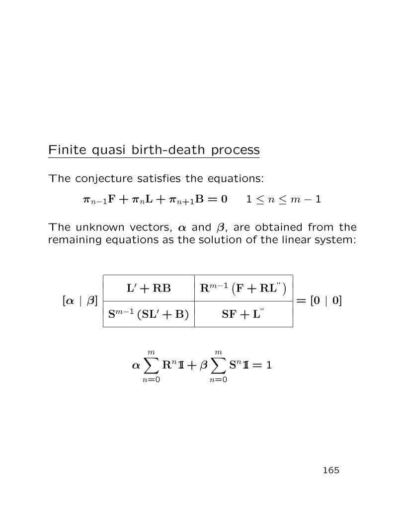
Finite quasi birth-death process

When the level process has an upper bound at level mthe generator matrix takes the form:

Q =

L′ F

B L . . .

B . . . F

. . . L F

B L”

Stationary equations:

π0L′ + π1B = 0

πn−1F + πnL + πn+1B = 0 1 ≤ n ≤ m− 1

πm−1F + πmL” = 0

m∑n=0

πn1I = 1

163

Finite quasi birth-death process

Due to the finite structure the stationary solution is notgeometric.

Conjecture:

We assume that the solution is a linear combination oftwo geometric series starting from the two bounds ofthe level process. I.e.,

πn = αRn + βSm−n, ∀0 ≤ n ≤ m,where matrix R and S are the solution of the matrixequations:

F + RL + R2B = 0

B + SL + S2F = 0

If in the homogeneous part the drift is

• negative: |λi(R)| < 1 and |λi(S)| ≤ 1,

• positive: |λi(R)| ≤ 1 and |λi(S)| < 1,

• zero: |λi(R)| ≤ 1 and |λi(S)| ≤ 1.

164

Finite quasi birth-death process

The conjecture satisfies the equations:

πn−1F + πnL + πn+1B = 0 1 ≤ n ≤ m− 1

The unknown vectors, α and β, are obtained from theremaining equations as the solution of the linear system:

[α | β]L′ + RB Rm−1

(F + RL”

)Sm−1 (SL′ + B) SF + L”

= [0 | 0]

αm∑n=0

Rn1I + βm∑n=0

Sn1I = 1

165

Finite quasi birth-death process

Computation ofm∑k=0

Rk (andm∑k=0

Sk):

• if |λi(R)| < 1, ∀i ∈ (1, . . . , n):

m∑k=0

Rk = (I−Rm+1)(I−R)−1

• if |λi(R)| ≤ 1, such that λ1(R) = 1

and |λi(R)| < 1, ∀i ∈ (2, . . . , n):

m∑k=0

Rk =

(I− (R−Π)m+1

)(I− (R−Π)

)−1

+mΠ

where

Π =uv

vu,

column vector u is a non-zero solution of

Ru = u

and row vector v is a non-zero solution of

vR = v .

Note that (R−Π)Π = Π(R−Π) = 0, Πi = Π and

Rk = ((R−Π) + Π)k = (R−Π)k+(R−Π)Π . . .︸ ︷︷ ︸0

+Πi

166

Piecewise constant infinite QBD with 2 parts

The process behaviour changes at level m:

Q =

0 1 · · · m−1 m m+1 · · ·L′ F

B L . . .

B . . . F

. . . L F

B L” F

B L F

B L . . .

. . . . . .

Stationary equations:

π0L′ + π1B = 0 n = 0

πn−1F + πnL + πn+1B = 0 1 ≤ n ≤ m− 1

πm−1F + πmL” + πm+1B = 0 n = m

πn−1F + πnL + πn+1B = 0 m+ 1 ≤ n∞∑n=0

πn1I = 1

167

Piecewise constant infinite QBD with 2 parts

Conjecture:

From levels 0 to m the solution is a linear combinationof two geometric series and from level m on it is matrixgeometric.

πn = αRn + βSm−n, 0 ≤ n ≤ m,

πn = πmRn−m = (αRm + β)Rn−m, m < n,

where matrices R, S and R are the solution of the matrixequations:

F + RL + R2B = 0

B + SL + S2F = 0

F + RL + R2B = 0

The conjecture satisfies the regular equations:

πn−1F + πnL + πn+1B = 0 1 ≤ n ≤ m− 1

πn−1F + πnL + πn+1B = 0 m+ 1 ≤ n

168

Piecewise constant infinite QBD with 2 parts

The unknown vectors, α and β, are obtained from theirregular equations (for level 0 and m) as the solution ofthe linear system:

[α | β] ·

L′ + RB Rm−1(F + R(L” + RB)

)Sm−1 (SL′ + B) SF + L” + RB

= [0 | 0]

αm−1∑n=0

Rn1I + βm−1∑n=0

Sn1I + (αRm + β)(I− R)−11I = 1

169

Piecewise constant finite QBD with 2 parts

Q =

0 1 · · · m−1 m m+1 · · · M−1 M

L′ F

B L . . .

B . . . F

. . . L F

B L” F

B L . . .

B . . . F

. . . L F

B L∗

Stationary equations:

π0L′ + π1B = 0 n = 0

πn−1F + πnL + πn+1B = 0 0 < n < m

πm−1F + πmL” + πm+1B = 0 n = m

πn−1F + πnL + πn+1B = 0 m < n < M

πm−1F + πmL∗ + πm+1B = 0 n = M∞∑n=0

πn1I = 1

170

Piecewise constant finite QBD with 2 parts

Conjecture:

πn = αRn + βSm−n, 0 ≤ n ≤ m,

πn = γRn−m + δSM−n, m ≤ n ≤M,

where matrices R, S and R, S are the solution of thematrix equations:

F + RL + R2B = 0, B + SL + S2F = 0,

F + RL + R2B = 0, B + SL + S2F = 0.

The conjecture satisfies the regular equations:

πn−1F + πnL + πn+1B = 0 0 < n < m

πn−1F + πnL + πn+1B = 0 m < n < M

171

Piecewise constant finite QBD with 2 parts

The unknown vectors, α, β, γ and δ, are obtained fromthe set of linear equations composed by the irregularequations (for level 0, m, m, M), where the two bound-ary equations for level m utilizes the two different formsof πm.

[α | β | γ | δ] ·

L′ + RB Rm−1(F+RL”

)Rm−1F 0

Sm−1(SL′+B) SF + L” SF 00 RB L” + RB RM−m−1

(F+RL∗

)0 SM−m−1B SM−m−1

(B+SL”

)SF + L∗

= [0 | 0 | 0 | 0]

αm−1∑n=0

Rn1I + βm−1∑n=0

Sn1I + γM−m∑n=0

Rn1I + δM−m∑n=0

Sn1I = 1

172

QBD with closed form solution

M/PH/1 queue:

Structure of the generator matrix:

Q =

−λ λα

a A−λI λI

aα A−λI λI

aα A−λI λI

. . . . . .

Stationary solution: πQ = 0, π1I = 1,

where π = π0,π1,π2, . . ..

Utilization: ρ = 1− π0 = λ E(PH) = λ α(−A)−11I

173

QBD with closed form solution

M/PH/1 queue balance equations:

− π0λ+ π1a = 0 (∗1)

π0λα+ π1(A−λI) + π2aα = 0 (∗2)

πn−1λI + πn(A−λI) + πn+1aα = 0 ∀n ≥ 2 (∗3)

First we show that

λπn1I = πn+1a ∀n ≥ 1. (∗4)

Substituting (∗1) it into (∗2) gives:

π1(aα+ A− λI) + π2aα = 0

Multiplying this with 1I from the right gives π1λ1I = π2a.Recursively substituting the result of the previous stepand multiplying (∗3) with 1I results in (∗4).

Substituting (∗4) into (∗3) gives:

λπn−1 + πn(A−λI) + λπn1Iα = 0 ∀n ≥ 2

and consequently

πn = πn−1 λ(λI−A− λ1Iα)−1︸ ︷︷ ︸R

∀n ≥ 2.

From (∗2) we also have π1 = π0αR.

−→ matrix geometric distribution:

πn = (1− ρ)αRn ∀n ≥ 1.

174

QBD with “closed” form solution

PH/M/1 queue:

Structure of the generator matrix:

Q =

A aα

µI A−µI aα

µI A−µI aα

µI A−λI aα

. . . . . .

Stationary solution: πQ = 0, π1I = 1,

where π = π0,π1,π2, . . ..

Utilization: ρ = 1− π01I =1

µ E(PH)=

1

µ α(−A)−11I

175

QBD with “closed” form solution

PH/M/1 queue balance equations:

π0A + π1µI = 0 (∗)

πn−1aα+ πn(A−µI) + πn+1µI = 0 ∀n ≥ 1 (∗∗)From (∗) we have π0 = µπ1(−A)−1.

The form of the stationary matrix geometric solution isπn = π0Rn where matrix R satisfies the matrix equation:

aα+ R(A−µI) + R2µ = 0.

Due to the fact that the first term, aα, is a diad matrixR is a diad as well in the form R = ar, where r is anunknown row vector. This diadic form results that r isproportional with πn, ∀n ≥ 1.

From (∗) and π0 = µπ1(−A)−1 we also have

π0A︸︷︷︸−µπ1

= −µπ0a︸︷︷︸µπ11I

r

and

r =π1

µπ11I.

176

QBD with “closed” form solution

Substituting these into (∗∗) with n = 1 gives:

µπ11Iα+ π1(A−µI) + µπ1ar = 0

and

π1 (µ1Iα+ A− µI) = −µπ1ar =−π1a

π11Iπ1.

That is, π1 is the left eigenvector of (µ1Iα+ A− µI)whose associated eigenvalue is the coefficient on theright hand side.

From πn = π1Rn−1 we have

π2 = π1ar =π1a

µπ11Iπ1 and πn = cn−1 π1,

where c = π1a/µπ11I.

From∑

nπn1I = 1 the normalizing condition for π1 is

π1

(µ(−A)−11I +

1

1− c1I

)= 1 .

177

QBD with “closed” form solution

On the other hand, multiplying (∗) with 1I from the rightresults

π0a = π1µ1I.

Recursively multiplying (∗∗) with 1I and substituting theprevious result gives

πn−1a = πnµ1I ∀n ≥ 1.

Substituting this into (∗∗) we have:

πnµ1Iα+ πn(A−µI) + πn+1µI = 0 ∀n ≥ 1

hence

πn+1 = πn (I−A/µ− 1Iα)︸ ︷︷ ︸this is not R!

∀n ≥ 1.

This relation does not hold for n = 0, but allows tocompute, e.g.

ρ =∞∑n=1

π1(I−A/µ− 1Iα)n−11I = π1(A/µ+ 1Iα)−11I

in closed form based on π1.

178

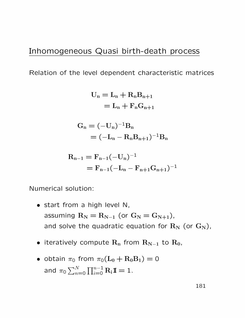
Inhomogeneous Quasi birth-death process

The transition rates (as well as level sizes) are leveldependent:

• Fn – (forward) transitions from level n to n+ 1

• Ln – (local) transitions in level n

• Bn – (backward) transitions from level n to n− 1.

Structure of the generator matrix:

Q =

L0 F0

B1 L1 F1

B2 L2 F2

B3 L3 F3

. . . . . .

On the block level it still has a birth-death structure,but with level dependent rates.

The stationary equations are

0 = π0L0 + π1B1

0 = πn−1Fn−1 + πnLn + πn+1Bn+1 for n ≥ 1

179

Inhomogeneous Quasi birth-death process

The level dependent characteristic matrices are:

• Rn – “ratio of time spent in level n and n+ 1”

• Gn – “return probability from level n to level n−1”

• Un – “generator of the restricted process on leveln”.

The stationary distribution has the form: πn+1 = πnRn

With this form the stationary equations become

0 = π0 (L0 + R0B1)

0 = πn−1 (Fn−1 + Rn−1Ln + Rn−1RnBn+1) for n ≥ 1

The level dependent analysis of the characteristic ma-trices gives

0 = Fn−1 + Rn−1Ln + Rn−1RnBn+1

0 = Bn + LnGn + FnGn+1Gn

Un = Ln + Fn(−Un+1)−1Bn+1

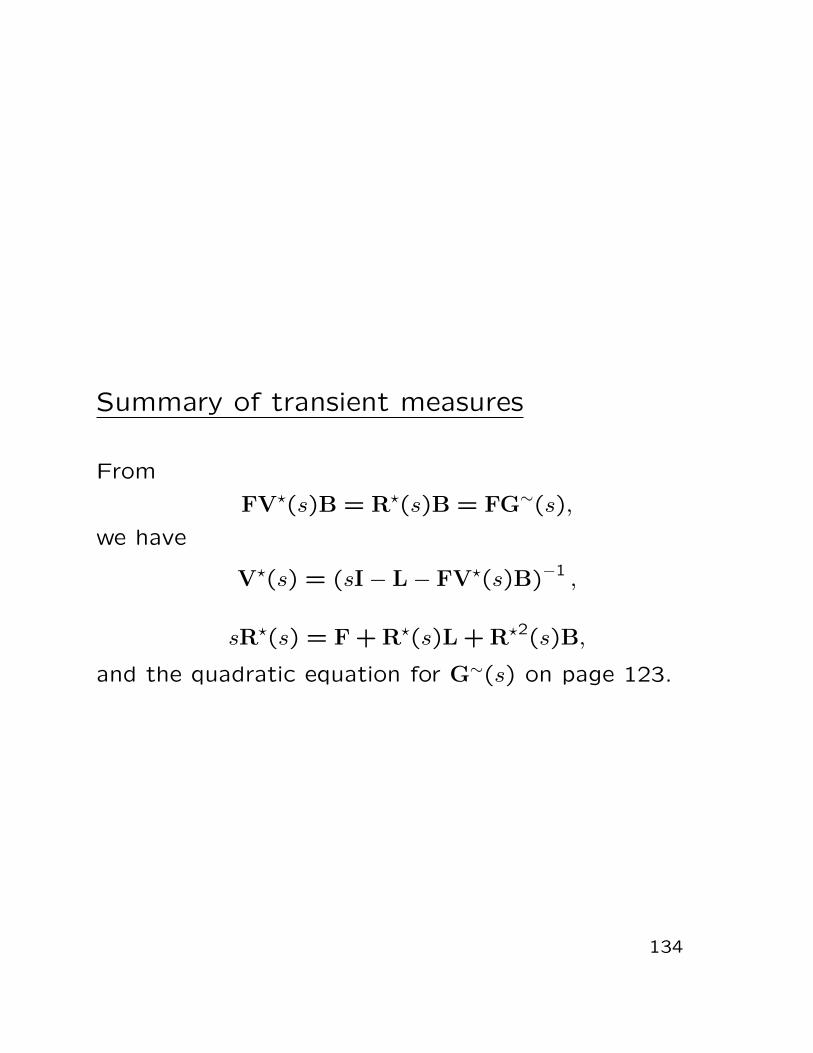
180

Inhomogeneous Quasi birth-death process

Relation of the level dependent characteristic matrices

Un = Ln + RnBn+1

= Ln + FnGn+1

Gn = (−Un)−1Bn

= (−Ln −RnBn+1)−1Bn

Rn−1 = Fn−1(−Un)−1

= Fn−1(−Ln − Fn+1Gn+1)−1

Numerical solution:

• start from a high level N,

assuming RN = RN−1 (or GN = GN+1),

and solve the quadratic equation for RN (or GN),

• iteratively compute Rn from RN−1 to R0,

• obtain π0 from π0(L0 + R0B1) = 0

and π0∑N

n=0

∏n−1i=0 Ri1I = 1.

181

G/M/1-type process

N(t), J(t) is a CTMC, where

• N(t) is the “level” process (e.g., number of cus-tomers in a queue),

• J(t) is the “phase” process (e.g., state of the en-vironment).

N(t), J(t) is a G/M/1-type process if upward transi-tions are restricted to one level up and there is no limiton downward transitions.

B1 ii

B1kk

B1 ii

B1kk

B1’jl

B2’kj B2kj

B1’ii

ijL’F’ji

F’ij

F’lj

L ij

Fji

Fij

Fjj

ijLF ij

Fji Fjj

ijL

i

j

i

j

L

k k

L’

l

i

j

L

k

i

j

L

k

Level 0 is irregular (e.g., no departure).

182

G/M/1-type process

Notation

• F – transitions one level up (e.g., arrival)

• L – transitions in the same level

• Bn – transitions n level down (e.g., departure)

• F′ – irregular block from level 0 to level 1.

• L′ – irregular block at level 0.

• B′n – irregular blocks down to level 0

Structure of the transition probability matrix:

Q =

L′ F′

B′1 L F

B′2 B1 L F

B′3 B2 B1 L F

... . . . . . . . . .

On the block level it has a G/M/1-type structure.

183

Condition of stability (G/M/1-type)

Asymptotically (n → ∞) the phase process is a CTMCwith generator matrix:

A = F + L +∞∑i=1

Bi

Assuming A is irreducible, the stationary solution of Ais:

αA = 0,α1I = 1

The stationary drift of the level process is:

d = αF1I−α∞∑i=1

i Bi 1I

Condition of stability:

d = αF1I−α∞∑i=1

i Bi 1I < 0

184

Matrix geometric distribution (G/M/1-type)

Stationary solution: πQ = 0, π1I = 1.

Partitioning π: π = π0,π1,π2, . . .

Decomposed stationary equations:

π0L′ +∞∑i=1

πiB′i = 0

π0F′ + π1L +∞∑i=1

πi+1Bi = 0

πn−1F + πnL +∞∑i=1

πn+iBi = 0 ∀n ≥ 2

∞∑n=0

πn1I = 1

Conjecture: πn = πn−1R, ∀n ≥ 1 → πn = π1Rn−1

where, matrix R is the solution of the matrix equation:

F + RL +∞∑i=1

Ri+1Bi = 0

185

Matrix geometric distribution (G/M/1-type)

The conjecture satisfies the equations:

πn−1F + πnL +∞∑i=1

πn+iBi = 0 ∀n ≥ 2

The remaining unknowns, π0 and π1, are the solutionof the linear system:

[π0|π1]

L′ F′

∞∑i=1

Ri−1B′i L +∞∑i=1

RiBi

= [ 0 | 0 ]

π01I + π1(I−R)−11I = 1

186

Matrix geometric distribution (G/M/1-type)

Linear algorithm to calculate R:

R := 0;REPEAT

Rold := R;

R := F

(−L−

∞∑i=1

RiBi

)−1

;

UNTIL||R−Rold|| ≤ ε

Linear algorithm to calculate R:

R := 0;REPEAT

Rold := R;

R :=

(−F−

∞∑i=1

Ri+1Bi

)L−1;

UNTIL||R−Rold|| ≤ ε

187

Matrix geometric distribution (G/M/1-type)

Properties of R:

• the matrix equation has more than one solution.

• if the G/M/1-type process is stable there is a so-lution R whose eigenvalues (λi(R)) are |λi(R)| < 1and this is the relevant R matrix.

• (if the G/M/1-type process is not stable there is asolution R whose eigenvalues (λi(R)) are |λi(R)| ≤1 and this is the relevant R matrix.)

Stochastic interpretation:

Rij is the ratio of the mean time spent in (n, j) and themean time spent in (n−1, i) before the first return tolevel n−1 starting from (n−1, i).

In a homogeneous G/M/1-type process Rij is indepen-dent of n.

188

Matrix geometric distribution (G/M/1-type)

Properties of the level crossing process:

• Matrix G cannot be used, because it is level depen-dent.

• Matrix U, remains level independent.

Interpretation of U :

The transient generator of the Markov chain restrictedto level n before the first visit to level n− 1.

Consequently −U−1 is the mean time spent in level nbefore the first visit to level n− 1.

U satisfies:

U = L +∞∑i=1

(F(−U)−1

)iBi = L +

∞∑i=1

RiBi.

189

M/G/1-type process

N(t), J(t) is a CTMC, where

• N(t) is the “level” process (e.g., number of cus-tomers in a queue),

• J(t) is the “phase” process (e.g., state of the en-vironment).

N(t), J(t) is an M/G/1-type process if downward tran-sitions are restricted to one level down and there is nolimit on upward transitions.

F1’lj

F1’ji

F1’ij

F2’jk F2 jk

Bii

F1ijijLBkk

F1jiF1jjF1jj

ijL

Bii

F1ijBkk

F1ji

ijL

B’jl

B’ii

ijL’

i

j

i

j

L

k k

L’

l

i

j

L

k

i

j

L

k

190

M/G/1-type process

Notation

• L – transitions in the same level

• B – transitions one level down (e.g., departure)

• Fn – transitions n level up (e.g., arrival)

• L′ – irregular block at level 0.

• B′ – irregular block from level 1 to level 0.

• F′n – irregular blocks starting from level 0

Structure of the transition probability matrix:

Q =

L′ F′1 F′2 F′3 F′4

B′ L F1 F2 F3

B L F1 F2

B L F1

. . . . . .

On the block level it has an M/G/1-type structure.

191

Condition of stability (M/G/1-type)

Asymptotically (n → ∞) the phase process is a CTMCwith generator matrix:

A = B + L +∞∑i=1

Fi

Assuming A is irreducible, the stationary solution of Ais:

αA = 0,α1I = 1

The stationary drift of the level process is:

d = α∞∑i=1

i Fi1I−αB 1I

Condition of stability:

d < 0

192

Stationary solution of M/G/1-type process

Stationary solution: πQ = 0, π1I = 1.

Decomposed stationary equations:

π0L′ + π1B′ = 0

π0F′n +n−1∑i=1

πiFn−i + πnL + πn+1B = 0 ∀n ≥ 1

∞∑n=0

πn1I = 1

Inhomogeneous dependency structure→ non-geometric solution

Invariant metric of the level process:matrix G (fundamental matrix)

B + LG +∞∑i=1

FiGi+1 = 0

193

Stationary solution of M/G/1-type process

Properties of G:

• the matrix equation has more than one solution.

• if the M/G/1-type process is stable G is a stochas-tic matrix,

• (if the M/G/1-type process is transient G is a sub-stochastic matrix.)

Stochastic interpretation:

Gij is the probability that starting from (n, i) the firststate visited in level n− 1 is (n− 1, j).

In a homogeneous M/G/1-type process Gij is indepen-dent of n.

(Matrix R cannot be used.)

(If B = γT · ν, where ν1I = 1, then G = 1I · ν.)

Matrix U satisfies

U = L +∞∑i=1

Fi

((−U)−1B︸ ︷︷ ︸

G

)i

194

Stationary solution of M/G/1-type process

Linear algorithm to calculate G:

G := I;REPEAT

Gold := G;

G :=

(−L−

∞∑i=1

FiGi

)−1

B;

UNTIL||G−Gold|| ≤ ε

Linear algorithm to calculate G:

G := I;REPEAT

Gold := G;

G := L−1

(−B−

∞∑i=1

FiGi+1

);

UNTIL||G−Gold|| ≤ ε

195

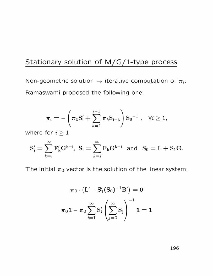
Stationary solution of M/G/1-type process

Non-geometric solution → iterative computation of πi:

Ramaswami proposed the following one:

πi = −

(π0S′i +

i−1∑k=1

πkSi−k

)S0−1 , ∀i ≥ 1,

where for i ≥ 1

S′i =∞∑k=i

F′kGk−i, Si =

∞∑k=i

FkGk−i and S0 = L + S1G.

The initial π0 vector is the solution of the linear system:

π0 ·(L′ − S′1(S0)−1B′

)= 0

π01I− π0

∞∑i=1

S′i

∞∑j=0

Sj

−1

1I = 1

196

Stationary solution of M/G/1-type process

Let us consider the restricted process on level 0 and 1:

Q(0,1) =L′ S′1

B′ S0

,

where S′1 contains all possible transitions from level 0 tolevel 1, S′1 =

∑∞k=1 F′kG

k−1, and S0 = U = L+∑∞

i=1 FiGi.

Further restricting the process to level 0,

Q(0) = L′ + S′1(−S0)−1B′ ,

from which

π0(L′ + S′1(−S0)−1B′) = 0.

From (π0,π1)Q(0,1) = 0 we have

π1 = π0S′1(−S0)−1 .

197

Stationary solution of M/G/1-type process

Similarly, let us consider the restricted process on level0, 1 and 2:

Q(0,1,2) =

L′ F′1 S′2

B′ L S1

B S0

where

• Sk describes the first transition from level ` (` ≥ 1)to level ` + k without visiting levels ` + 1 through`+ k − 1.

• S′k describes the first transition from level 0 to levelk without visiting levels 1 through k − 1.

From (π0,π1,π2)Q(0,1,2) = 0 we have

π2 =(π0S′2 + π1S1

)(−S0)−1 .

Level by level increasing the size of the restricted processwe obtain the Ramaswami formula.

198

Stationary solution of M/G/1-type process

We introduce an artificial infinite block structure of eachlevels to compose a QBD process.

block 0

block 1

block 2

B’ B

F’1 F1 F1

F’2 F2 F2

20 1levelL’ L L

I I

I I

199

Stationary solution of M/G/1-type process

Block structure of the infinite phase QBD process

Q′ =

L′ F

B′ L F

B L F

B L F

. . . . . .

, F =I

I

. . .

,

L′ =

L′ F′1 F′2 · · ·

−I

−I

. . .

, B′ =

B′

,

L =

L F1 F2 · · ·

−I

−I

. . .

, B =

B

.

200

Stationary solution of M/G/1-type process

At level 0 we have the stationary equation

0 = π′0L′ + π′1B.

The partitioned form of this equation is

0 = π′0,0L′ + π′1,0B′, block 0, (0*)

0 = −π′0,iI + π′0,0F′i, block i. (0**)

201

Stationary solution of M/G/1-type process

Form the transition structure of the QBD process wehave

G =

G

G2

G3

...

.

Restricting the QBD proces to the first n levels gives

Q′n =

L′ F

B′ L . . .

B . . . F

. . . L F

B L+FG

,

202

Stationary solution of M/G/1-type process

where

FG =

0

G

G2

...

,

and

L+FG =

L F1 F2 · · ·

G −I

G2 −I

... . . .

,

from which

0 = π′n−1F + π′n(L+FG).

The partitioned form of this equation is

0 = π′n−1,1 + π′n,0L +∞∑k=1

π′n,kGk, block 0, (*)

0 = π′n−1,i+1 − π′n,i + π′n,0Fi, block i. (**)

203

Stationary solution of M/G/1-type process

From (**) we have

π′n,i = π′n−1,i+1 + π′n,0Fi.

Substituting π′n,i into (*) we have

0 = π′n−1,1 + π′n,0L +∞∑k=1

π′n−1,k+1Gk +∞∑k=1

π′n,0FkGk,

= π′n,0

(L +

∞∑k=1

FkGk

)+

∞∑k=0

π′n−1,k+1Gk,

from which

π′n,0 = −

( ∞∑k=0

π′n−1,k+1Gk

)(L +

∞∑i=1

FiGi

)−1

︸ ︷︷ ︸S0−1

. (∗ ∗ ∗)

204

Stationary solution of M/G/1-type process

Now, we look for a recursive evaluation of π′n−1,i+1.

Applying (**) for block i+ 1 and level n− 1 we have

π′n−1,i+1 = π′n−2,i+2 + π′n−1,0Fi+1 ,

and similarly

π′n−2,i+2 = π′n−3,i+3 + π′n−2,0Fi+2 ,

Repeatedly applying this up to level 0 we have:

π′n−1,i+1 = π′0,i+n +n−1∑j=1

π′n−j,0Fi+j .

and using π′0,i+j = π′0,0F′i+j from (0**) we have

π′n−1,i+1 = π′0,0F′i+n +n−1∑j=1

π′n−j,0Fi+j .

205

Stationary solution of M/G/1-type process

Substituting this into (***) we have

π′n,0 = −

( ∞∑i=0

π′n−1,i+1Gi

)S0−1 =

= −

( ∞∑i=0

π′0,0F′i+nGi

)S0−1

−

∞∑i=0

n−1∑j=1

π′n−j,0Fi+jGi

S0−1 =

= −(π′0,0S′n

)S0−1 −

n−1∑j=1

π′n−j,0Sj

S0−1

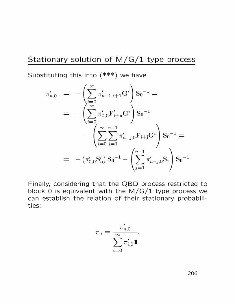
Finally, considering that the QBD process restricted toblock 0 is equivalent with the M/G/1 type process wecan establish the relation of their stationary probabili-ties:

πn =π′n,0∞∑i=0

π′i,01I

.

206

Computation of π0

Let Q0 be the generator of restricted CTMC of theoriginal M/G/1-type process on level 0.

Q0 = L′ +∞∑k=1

F′kPk→0,

where

Pk→0 = Pr(J(γ0) | X(0) = k, J(0)).

From the regular structure of the k ≥ 1 levels we havePk→0 = Gk−1P1→0 and similar to the equation definingmatrix G matrix P1→0 satisfies

B′ + LP1→0 +∞∑k=1

FkGkP1→0 = 0,

from which

P1→0 = −(L +∞∑k=1

FkGk)−1B′ = −S0

−1B′

and

Q0 = L′ +∞∑k=1

F′kGk(−S0)−1B′ = L′ + S′1(−S0)−1B′.

π0 satisfies π0Q0 = 0.

207

Normalizing π0

From

πi =

(π0S′i +

i−1∑k=1

πkSi−k

)(−S0)−1 , ∀i ≥ 1,

assuming S′0 = 0, S′(z) =∑∞

i=0 S′izi and S(z) =

∑∞i=0 Siz

i

we have

π(z) =∑∞

i=0πizi =

π0 + π0S′(z)(−S0)−1 + (π(z)− π0)(S(z)− S0)(−S0)−1

and than

π(z) = π0

(I− S′(z)S(z)−1

).

The normalizing equation is

1 =∞∑i=0

πi1I = π(1)1I = π01I− π0S′(1)(S(1))−1 1I

= π01I− π0

( ∞∑i=1

S′i

) ∞∑j=0

Sj

−1

1I.

208

Normalizing π0

Without introducing the transforms we have

∞∑i=1

πi =∞∑i=1

π0S′i(−S0)−1 +∞∑i=1

i−1∑k=1

πkSi−k(−S0)−1,

= π0

∞∑i=1

S′i(−S0)−1 +

( ∞∑k=1

πk

)( ∞∑i=1

Si

)(−S0)−1,

Multiplying with −S0 from the left gives

∞∑i=1

πi

(−S0 −

∞∑i=1

Si

)= π0

∞∑i=1

S′i

from which we obtain the same normalizing equation

1 = π01I− π0

( ∞∑i=1

S′i

) ∞∑j=0

Sj

−1

1I.

209

MAP/G/1 queue

(based on ”Lucantoni: New results ...” paper )

Special case:the M/G/1-type structure is resulted by a BMAP/G/1queue with:

• BMAP arrival process: D0,D1,D2, . . .

• (general) service time distribution: H(t)

Notations:

• number of arrivals in (0, t): N(t)

• D =∞∑i=0

Di, D(z) =∞∑i=0

Dizi

• arrival intensity: λ = γ∞∑k=1

kDk1I, where γ is the

solution of γD = 0,γ1I = 1

• utilization: ρ = λ/µ (1/µ is the mean service time)

• Pij(n, t) = Pr(N(t) = n, J(t) = j | J(0) = i)

P(z, t) = eD(z)t

210

MAP/G/1 queue

Stationary queue length at departure

Embedded DTMC:

P =

B0 B1 B2 B3 . . .

A0 A1 A2 A3 . . .

A0 A1 A2 . . .

A0 A1 . . .

. . . . . .

• [An]ij =Pr(phase moves from i to j and there are n arrivalsduring a service)

• [Bn]ij =Pr(phase moves from i to j and there are n+ 1arrivals during an arrival and a service)

211

MAP/G/1 queue

An =

∫ ∞t=0

P(n, t)dH(t), Bn = −D0−1

n∑k=0

Dk+1An−k.

A(z) =∞∑n=0

zn An =∞∑n=0

zn∫ ∞t=0

P(n, t)dH(t)

=

∫ ∞t=0

P(z, t)dH(t) =

∫ ∞t=0

eD(z)tdH(t)

B(z) = −D0−1[D(z)−D0] z−1A(z).

212

MAP/G/1 queue

Stationary equation of the embedded process:

πi = π0Bi +i+1∑k=1

πkAi+1−k, i ≥ 0

Multiplying the ith equation with zi and summing upgives:

π(z) = π0B(z) + z−1(π(z)− π0)A(z).

and the queue length distribution at departure is:

π(z)

(zI−A(z)

)= π0

(zB(z)−A(z)

)= π0(−D0)−1D(z)A(z),

(∗)

Let G(z) =∑∞

n=0 znG(n) where

Gij(n) = Pr(Jγ0 = j, γ0 = n | J0 = i, N0 = 1)

Transition from level i (i ≥ 1) to level i−1:

G(z) = z

∞∑k=0

AkGk(z), G =

∞∑k=0

AkGk.

Transition from level 0 to level 0:

K(z) = z

∞∑k=0

BkGk(z), K =

∞∑k=0

BkGk.

213

MAP/G/1 queue

The unknown vector, π0, is calculated based on thestationary solution of the restricted process on level 0(κ) and the mean time to return to level 0 (κ∗):

π0 =κ

κκ∗

where κ is the solution of κK = κ, κ1I = 1, and thenormalizing constant is computed from the mean timeto return to level 0,

κ∗ =d

dzK(z)1I

∣∣∣∣z=1

.

π0 can also be normalized based on z → 1 in (∗).

214

MAP/G/1 queue

Computation of κ∗

κ∗ =d

dzK(z)1I

∣∣∣∣z=1

=d

dzz

∞∑k=0

BkGk(z)1I

∣∣∣∣∣z=1

=∞∑k=0

Bk Gk1I︸︷︷︸1I︸ ︷︷ ︸

1I

+∞∑k=0

Bkd

dzGk(z)1I|z=1

=∞∑k=0

Bk Gk1I︸︷︷︸1I︸ ︷︷ ︸

1I

+∞∑k=0

Bk

k−1∑j=0

Gj

︸ ︷︷ ︸(∗)

G(1) Gk−j−11I︸ ︷︷ ︸1I

.

(∗) closed form expression is given at finite QBDs.

215

MAP/G/1 queue

Computation of the last term, G(1)1I

G(1)1I =d

dzG(z)1I|z=1 =

d

dzz

∞∑k=0

AkGk(z)1I

∣∣∣∣∣z=1

=

=∞∑k=0

AkGk1I︸ ︷︷ ︸

1I

+∞∑k=1

Akd

dzGk(z)1I|z=1 =

= 1I +∞∑k=1

Ak

k−1∑j=0

GjG(1)Gk−j−11I =

= 1I +∞∑k=1

Ak

k−1∑j=0

Gj

︸ ︷︷ ︸(∗)

G(1)1I =

(∗) closed form expression.

216

MAP/G/1 queue

Stationary queue length distribution at arbitrary time:

The (N(t), J(t)) process of a MAP/G/1 queue is aMarkov regenerative process with embedded points atdepartures.

The stationary distribution (ψ(z)) can be computed basedon the embedded distribution (π(z)) and the mean timespent in different state in a regenerative period.

Tij(k, `) =E(time in (`, j) in a reg. period | N(0) = k, J(0) = i)

For k ≤ `, k > 0

T(k, `) =

∫ ∞t=0

P(`− k, t) (1−H(t)) dt .

For ` = k = 0

T(0,0) =

∫ ∞t=0

eD0t dt = (−D0)−1 .

For k = 0, ` > 0

T(0, `) =∑k=1

(−D0)−1Dk︸ ︷︷ ︸1st arrival

∫ ∞t=0

P(`−k, t) (1−H(t)) dt .

217

MAP/G/1 queue

From Markov regenerative theory

ψ` =

∑k=0

πkT(k, `)

∞∑k=0

πk

∞∑n=k

T(k, n)1I

= λ∑k=0

πkT(k, `) ,

where the denominator is the mean time of a regenera-tive period, i.e., mean inter-departure time. When thesystem is stable it equals to the mean inter-arrival time,1/λ.

For ` = 0 we have

ψ0 = λπ0(−D0)−1

which satisfies ψ01I = 1 − ρ, since π0(−D0)−11I is themean idle time in a regeneration period.

218

MAP/G/1 queue

For ` > 0 we multiply with z` and sum up from 1 to ∞

ψ(z)− ψ0 =

λπ0(−D0)−1(D(z)−D0)

∫ ∞t=0

P(z) (1−H(t)) dt +

λ(π(z)− π0)

∫ ∞t=0

P(z) (1−H(t)) dt =

λ

(π0(−D0)−1D(z) + π(z)

)∫ ∞t=0

P(z) (1−H(t)) dt ,

where ∫ ∞t=0

P(z)(1−H(t)) dt =∫ ∞t=0

eD(z)t dt−∫ ∞t=0

eD(z)tH(t) dt =∫ ∞t=0

eD(z)t dt−∫ ∞t=0

(−D(z))−1eD(z)t dH(t) =

(−D(z))−1(I−A(z)) .

Note that, D(z) and A(z) commutes.

219

MAP/G/1 queue

ψ(z)− ψ0 =

λ

(π0(−D0)−1D(z) + π(z)

)(−D(z))−1(I−A(z)) =

λ

(− π0(−D0)−1︸ ︷︷ ︸

−ψ0

+π(z)(−D(z))−1

)(I−A(z)) =

− ψ0 + λπ0(−D0)−1A(z) + λπ(z)(−D(z))−1(I−A(z))

Simplifying with ψ0 and substituting π0(−D0)−1D(z)A(z)according to (∗), using that D(z) and A(z) commutes,gives

ψ(z) = λπ(z)(zI−A(z))(D(z))−1 +

λπ(z)(−D(z))−1(I−A(z)),

and we finally get

ψ(z)D(z) = λ(z − 1)π(z).

The inverse transformation gives

ψ`+1 =

(∑k=0

ψkD`+1−k − λ(π` − π`+1)

)(−D0)−1 .

220

Fluid models

A simple function of the current state of a discrete statestochastic process, S(t), governs the evolution of a con-tinuous variable X(t).

When the discrete state stochastic process is a CTMC

• S(t), X(t) is a Markov process ⇒ Markov fluidmodel.

Fluid models: bounded evolution of the continuous vari-able.

S(t)

k

i

j

t

t

X(t)

r

irkr kr

j

B

0

221

Classes of fluid models

• finite buffer – infinite buffer,

• first order – second order,

• homogeneous – fluid level dependent,

• barrier behaviour in second order case

– reflecting – absorbing.

222

Buffer size

Infinite buffer: X(t) is only lower bounded at zero.

Finite buffer: X(t) is lower bounded at zero and upperbounded at B.

S(t)

k

i

j

t

t

X(t)

r

irkr kr

j

0

S(t)

k

i

j

t

t

X(t)

r

irkr kr

j

B

0

223

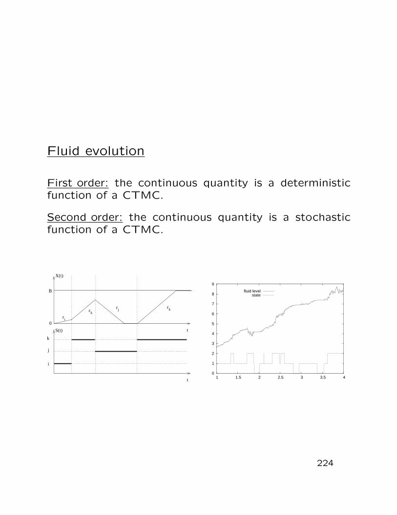
Fluid evolution

First order: the continuous quantity is a deterministicfunction of a CTMC.

Second order: the continuous quantity is a stochasticfunction of a CTMC.

S(t)

k

i

j

t

t

X(t)

r

irkr kr

j

B

0

0

1

2

3

4

5

6

7

8

9

1 1.5 2 2.5 3 3.5 4

fluid levelstate

224

Interpretation of second order fluid models

Random walk with decreasing time and fluid granularity.

CTMC state

Fluid

level

225

Dependence on fluid level

Homogeneous: the evolution of the CTMC is indepen-dent of the fluid level.

Fluid level dependent: the generator of the CTMC is afunction of the fluid level.

dX(t) =rdt

S(t)

Q

X(t)

S(t)

X(t)

S(t)

Q(X(t))

dX(t) =rdt

S(t)(X(t))

226

Boundary behaviour of second order fluid models

Reflecting: the fluid level is immediately reflected at theboundary.

Absorbing: the fluid level remains at the boundary up toa state transition of the Markov chain.

t

X(t)

S(t)

k

i

j

t

r=0iσ kr

B

j

>0

<0

t

X(t)

S(t)

k

i

j

t

r=0iσ kr

B

j

>0

<0

227

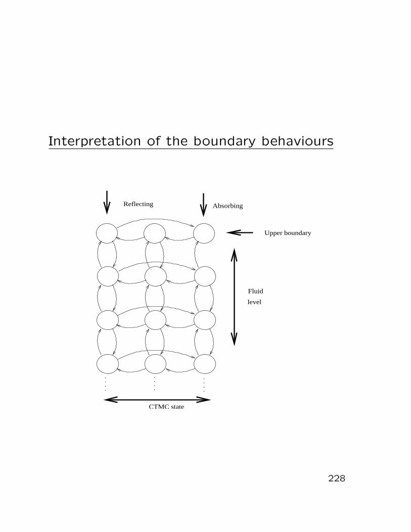
Interpretation of the boundary behaviours

CTMC state

Fluid

level

Upper boundary

Reflecting Absorbing

228

Transient behaviour of fluid models

First order, infinite buffer, homogeneous case

During a sojourn of the CTMC in state i (S(t) = i) thefluid level (X(t)) increases at rate ri when X(t) > 0:

X(t+ ∆)−X(t) = ri∆ if S(t) = i,X(t) > 0.

that is

d

dtX(t) = ri if S(t) = i,X(t) > 0.

When X(t) = 0 the fluid level can not decrease:

d

dtX(t) = max(ri,0) if S(t) = i,X(t) = 0.

That is

d

dtX(t) =

rS(t) if X(t) > 0,

max(rS(t),0) if X(t) = 0.

229

Transient behaviour with finite buffer

When X(t) = B the fluid level can not increase:

d

dtX(t) = min(ri,0), if S(t) = i,X(t) = B.

That is

d

dtX(t) =

rS(t), if X(t) > 0,max(rS(t),0), if X(t) = 0,min(rS(t),0), if X(t) = B.

230

3.2 Transient behaviour of fluid models

Second order, infinite buffer, homogeneous Markov fluidmodels with reflecting barrier

During a sojourn of the CTMC in state i (S(t) = i) in thesufficiently small (t, t+∆) interval the distribution of thefluid increment (X(t+ ∆)−X(t)) is normal distributedwith mean ri∆ and variance σ2

i ∆:

X(t+ ∆)−X(t) = N (ri∆, σ2i ∆),

if S(u) = i, u ∈ (t, t+ ∆), X(t) > 0.

At X(t) = 0 the fluid process is reflected immediately,

−→ Pr(X(t) = 0) = 0.

231

3.2 Transient behaviour of fluid models

Second order, infinite buffer, homogeneous Markov fluidmodels with absorbing barrier

Between the boundaries the evolution of the process isthe same as before.

First time when the fluid level decreases to zero the fluidprocess stops,

−→ Pr(X(t) = 0) > 0.

Due to the absorbing property of the boundary the prob-ability that the fluid level is close to it is very low,

−→ lim∆→0Pr(0<X(t)<∆)

∆= 0.

232

3.2 Transient behaviour of fluid models

Inhomogeneous (fluid level dependent), first order, infi-nite buffer Markov fluid models

The evolution of the fluid level is the same:

d

dtX(t) =

rS(t)(X(t)), if X(t) > 0,

max(rS(t)(X(t)),0), if X(t) = 0.

But the evolution of the CTMC depends on the fluidlevel:

lim∆→0

Pr(S(t+ ∆) = j|S(t) = i)

∆= qij(X(t)) .

The generator of the CTMC is Q(X(t)) and the rate

matrix is R(X(t)).

233

3.3 Transient description of fluid models

Notations:

πi(t) = Pr(S(t) = i) – state probability,

ui(t) = Pr(X(t) = B,S(t) = i) – buffer full probability,

`i(t) = Pr(X(t) = 0, S(t) = i) – buffer empty probability,

pi(t, x) = lim∆→0

1

∆Pr(x < X(t) < x+ ∆, S(t) = i)

– fluid density.

=⇒ πi(t) = `i(t) + ui(t) +∫xpi(t, x)dx.

234

3.3 Transient description of fluid models

First order, infinite buffer, homogeneous behaviour.

Forward argument:

If S(t+ ∆) = i, then between t and t+ ∆ the CTMC

• stays in i with probability 1 + qii∆,

• moves from k to i with probability qki∆,

• has more than 1 state transition with probabilityσ(∆).

235

3.3 Transient description of fluid models

Fluid density:

pi(t+ ∆, x) = (1 + qii∆) pi(t, x− ri∆)+∑k∈S,k 6=i

qki∆ pk(t, x−O(∆))+

σ(∆) ,

where lim∆→0 σ(∆)/∆ = 0 and lim∆→0O(∆) = 0.

236

3.3 Transient description of fluid models

pi(t+ ∆, x)− pi(t, x− ri∆) =∑k∈S

qki∆ pk(t, x−O(∆)) + σ(∆) ,

pi(t+ ∆, x)− pi(t, x)

∆+ ri

pi(t, x)− pi(t, x− ri∆)

ri∆=∑

k∈S

qki pk(t, x−O(∆)) +σ(∆)

∆,

∂

∂tpi(t, x) + ri

∂

∂xpi(t, x) =

∑k∈S

qki pk(t, x) .

237

3.3 Transient description of fluid models

Empty buffer probability:

If ri > 0,

−→ the fluid level increases in state i,

−→ `i(t) = Pr(X(t) = 0, S(t) = i) = 0.

238

3.3 Transient description of fluid models

If ri ≤ 0:

`i(t+ ∆) =

(1 + qii∆)

(`i(t) +

∫ −ri∆0

pi(t, x)dx︸ ︷︷ ︸∗

)+

∑k∈S,k 6=i

qki∆

(`k(t) +

∫ O(∆)

0pk(t, x)dx︸ ︷︷ ︸O(∆)

)+

σ(∆) .

239

3.3 Transient description of fluid models

When x ≤ −ri∆, then

pi(t, x) = pi(t,0) + xp′i(t,0) + σ(∆) ,

and

∗ =

∫ −ri∆0

pi(t, x)dx

=

∫ −ri∆0

pi(t,0)dx+

∫ −ri∆0

xp′i(t,0)dx+

∫ −ri∆0

σ(∆)dx

= −ri∆ pi(t,0) +(−ri∆)2

2p′i(t,0)︸ ︷︷ ︸

σ(∆)

+ (−ri∆) σ(∆)︸ ︷︷ ︸σ(∆)

.

240

3.3 Transient description of fluid models

From which the empty buffer probability:

`i(t+ ∆) = (1 + qii∆)(`i(t) −ri∆pi(t,0) + σ(∆)

)+∑

k∈S,k 6=i

qki∆ (`k(t) +O(∆)) + σ(∆) ,

`i(t+ ∆)− `i(t) = qii∆ `i(t)− ri∆pi(t,0)+∑k∈S,k 6=i

qki∆ (`k(t) +O(∆)) + σ(∆) ,

241

3.3 Transient description of fluid models

and

`i(t+ ∆)− `i(t)∆

=

− ri pi(t,0) +∑k∈S

qki (`k(t) +O(∆)) +σ(∆)

∆,

d

dt`i(t) = −ri pi(t,0) +

∑k∈S

qki `k(t) .

242

3.3 Transient description of fluid models

Set of governing equations:

Fluid density:

∂

∂tpi(t, x) + ri

∂

∂xpi(t, x) =

∑k∈S

qki pk(t, x) ,

Empty buffer probability:

if ri <= 0:

d

dt`i(t) = −ri pi(t,0) +

∑k∈S

qki `k(t),

if ri > 0:

`i(t) = 0.

243

3.3 Transient description of fluid models

By the definition of fluid density and empty buffer prob-ability: ∫ ∞

0pi(t, x)dx+ `i(t) = πi(t) .

In the homogeneous case:

d

dtπi(t) =

∑k∈S

qki πk(t), −→ πi(t) = πi(0)eQt.

244

3.3 Transient description of fluid models

First order, finite buffer , homogeneous behaviour.

If there is also an upper boundary:

if ri < 0:

ui(t) = 0,

if ri ≥ 0:

d

dtui(t) = ri pi(t, B) +

∑k∈S

qki uk(t).

245

3.3 Transient description of fluid models

Second order , infinite buffer, homogeneous behaviour.

Fluid density:

pi(t+ ∆, x) =

(1 + qii∆)

∫ ∞−∞

pi(t, x− u)fN (∆ri,∆σ2i )

(u)du︸ ︷︷ ︸∗∗

+

∑k∈S,k 6=i

qki∆ pk(t, x−O(∆))+

σ(∆)

246

3.3 Transient description of fluid models

Using

pi(t, x− u) = pi(t, x)− up′i(t, x) +u2

2p′′i (t, x) +O(u)3

we have:

∗∗ =

pi(t, x)

∫ ∞−∞

fN (∆ri,∆σ2i )

(u)du︸ ︷︷ ︸1

−p′i(t, x)

∫ ∞−∞

ufN (∆ri,∆σ2i )

(u)du︸ ︷︷ ︸∆ri

+

p′′i (t, x)

∫ ∞−∞

u2

2fN (∆ri,∆σ2

i )(u)du︸ ︷︷ ︸

∆2r2i +∆σ2

i /2=∆σ2i /2+σ(∆)

+

∫ ∞−∞O(u)3fN (∆ri,∆σ2

i )(u)du︸ ︷︷ ︸

O(∆)2=σ(∆)

.

247

3.3 Transient description of fluid models

From which:

pi(t+ ∆, x) =

(1 + qii∆)(pi(t, x)− p′i(t, x)∆ri + p′′i (t, x)∆σ2

i /2)

+∑k∈S,k 6=i

qki∆ pk(t, x−O(∆)) + σ(∆) ,

pi(t+ ∆, x)− pi(t, x) =qii∆pi(t, x)− p′i(t, x)∆ri + p′′i (t, x)∆σ2

i /2+∑k∈S,k 6=i

qki∆ pk(t, x−O(∆)) + σ(∆) ,

∂

∂tpi(t, x) +

∂

∂xpi(t, x)ri −

∂2

∂x2pi(t, x)

σ2i

2=∑k∈S

qki pk(t, x).

248

3.3 Transient description of fluid models

Second order , infinite buffer, reflecting barrier , homo-geneous behaviour.

Boundary condition:

Reflecting barrier −→ `i(t) = 0.

Fluid density at 0:∫ ∞0

pi(t, x)dx = πi(t)

/∂

∂t

249

3.3 Transient description of fluid models

∫ ∞x=0

∂

∂tpi(t, x)︸ ︷︷ ︸︷ ︸︸ ︷

−∂pi(t, x)

∂xri +

∂2pi(t, x)

∂x2

σ2i

2+∑k∈S

qki pk(t, x)

dx =∂

∂tπi(t)︸ ︷︷ ︸︷ ︸︸ ︷∑

k∈S

qkiπi(t)

−ri[pi(t, x)

]∞x=0︸ ︷︷ ︸

−pi(t,0)

+σ2i

2

[p′i(t, x)

]∞x=0︸ ︷︷ ︸

−p′i(t,0)

+∑k∈S

qki

∫ ∞x=0pk(t, x)dx︸ ︷︷ ︸πi(t)

=∑k∈S

qkiπi(t)

ripi(t,0)−σ2i

2p′i(t,0) = 0

250

3.3 Transient description of fluid models

First order, infinite buffer, inhomogeneous behaviour .

Fluid density:

∂

∂tpi(t, x) + ri(x)

∂

∂xpi(t, x) =

∑k∈S

qki(x) pk(t, x)

Empty buffer probability:

if ri(0) < 0 (and ri(x) is continuous):

d

dt`i(t) = − ri(0) pi(t,0) +

∑k∈S

qki(0) `k(t),

if ri(0) > 0 (and ri(x) is continuous):

`i(t) = 0.

251

3.3 Transient description of fluid models

General case:

Second order , finite buffer , inhomogeneous behaviour .

Differential equations:

∂p(t, x)

∂t+∂p(t, x)

∂xR(x) −

∂2p(t, x)

∂x2S(x) = p(t, x) Q(x) ,

p(t,0) R(0) − p′(t,0) S(0) = `(t) Q(0) ,

−p(t, B) R(B) + p′(t, B) S(B) = u(t) Q(B) ,

where R(x) = Diag〈ri(x)〉 and S(x) = Diag〈σ2i (x)2〉.

252

3.3 Transient description of fluid models

General case:

Second order , finite buffer , inhomogeneous behaviour .

Bounding behaviour:

σi = 0 and positive/negative drift: `i(t)=0/ui(t)=0.

σi>0 , reflecting lower/upper barrier: `i(t) = 0/ui(t) =0.

σi>0 , absor. lower/upper barrier: pi(t,0)=0/pi(t, B)=0.

Normalizing condition:∫ B

0p(t, x) dx1I + `(t)1I + u(t)1I = 1.

253

3.4 Stationary description of fluid models

Condition of ergodicity:

For ∀x, y ∈ R+, ∀i, j ∈ S the transition time

T = mint>0

(X(t) = y, S(t) = j|X(0) = x, S(0) = i)

has a finite mean (i.e., E(T ) <∞).

254

3.4 Stationary description of fluid models

Notations:

πi = limt→∞

Pr(S(t) = i) – state probability,

ui = limt→∞

Pr(X(t) = B,S(t) = i) – buffer full probability,

`i = limt→∞

Pr(X(t) = 0, S(t) = i) – buffer empty probabil-

ity,

pi(x) = limt→∞

lim∆→0

1

∆Pr(x < X(t) < x+ ∆, S(t) = i)

– fluid density,

Fi(x) = limt→∞

Pr(X(t) < x, S(t) = i)

– fluid distribution.

255

3.4 Stationary description of fluid models

First order, infinite buffer, homogeneous behaviour.

Fluid density:

ri∂

∂xpi(x) =

∑k∈S

qki pk(x) .

Empty buffer probability:

if ri <= 0:

0 = −ri pi(0) +∑k∈S

qki `k,

if ri > 0:

`i = 0.

256

3.4 Stationary description of fluid models

First order, finite buffer , homogeneous behaviour.

Fluid density:

ri∂

∂xpi(x) =

∑k∈S

qki pk(x) .

Boundary equations: ri pi(0) =∑k∈S

qki `k, if ri ≤ 0,

`i = 0, if ri > 0. −ri pi(B) =∑k∈S

qki uk, if ri ≥ 0,

ui = 0, if ri < 0.

257

3.4 Stationary description of fluid models

Second order , infinite buffer, reflecting boundary , ho-mogeneous behaviour.

Fluid density:

ri∂

∂xpi(x)−

∂2

∂x2pi(x)

σ2i

2=∑k∈S

qki pk(x) .

Empty buffer probability:

`i = 0.

Boundary equation:

ripi(0)−σ2i

2p′i(0) =

∑k∈S

qki `k = 0.

258

3.4 Stationary description of fluid models

Second order , infinite buffer, absorbing boundary , ho-mogeneous behaviour.

Fluid density:

ri∂

∂xpi(x)−

∂2

∂x2pi(x)

σ2i

2=∑k∈S

qki pk(x).

Empty buffer probability:

pi(0) = 0.

Boundary equation:

−σ2i

2p′i(0) =

∑k∈S

qki `k.

259

3.4 Stationary description of fluid models

General case:

Second order , finite buffer , inhomogeneous behaviour .

p′(x) R(x) − p′′(x) S(x) = p(x) Q(x) ,

p(0) R(0) − p′(0) S(0) = ` Q(0) ,

−p(B) R(B) + p′(B) S(B) = u Q(B) ,

σi=0 and positive/negative drift: `i = 0/ui = 0.

σi>0, reflecting lower/upper barrier: `i = 0/ui = 0.

σi>0, absorbing lower/upper barrier: pi(0) = 0/pi(B) =0.

260

4 Solution methods

Numerical techniques:

reward fluiddifferential equations (+) +

spectral decomposition (+) +randomization + +

transform domain + +matrix exponent + +

moments + -

261

4 Solution methods

Transient analysis:

• initial condition ,

• set of differential equations,

• bounding behaviour.

Stationary analysis:

• set of differential equations,

• bounding behaviour,

• normalizing condition .

262

4.1 Transient solution methods

• Numerical solution of differential equations,

• Randomization,

• Markov regenerative approach,

• Transform domain.

263

4.1 Transient solution methods

Numerical solution of differential equations (Chen et al.)

All cases.

The approach

• starts from the initial condition, and

• follows the evolution of the fluid distribution in the(t, t+ ∆) interval at some fluid levels based on thedifferential equations and the boundary condition.

This is the only approach for inhomogeneous models.

264

4.1 Transient solution methods

Randomization (Sericola)

First order, infinite buffer, homogeneous behaviour.

F ci (t, x) =

∞∑n=0

e−λt(λt)n

n!

n∑k=0

(nk

)xkj(1− xj)n−kb(j)

i (n, k),

where F ci (t, x) = Pr(X(t) > x, S(t) = i),

xj =x−r+

j−1t

rjt−r+j−1t

if x ∈ [r+j−1t, rjt), and

b(j)i (n, k) is defined by initial value and a simple recur-

sion.

265

4.1 Transient solution methods

Properties of the randomization based solution method:

• the expression with the given recursive formulas isa solution of the differential equation,the initial value of b(j)

i (n, k) is set to fulfill the bound-ary condition,

• 0 ≤ xj ≤ 1−→ convex combination of non-negative numbers−→ numerical stability,

• the initial fluid level is X(0) = 0.(extension to X(0) > 0 and to finite buffer is notavailable.)

266

4.1 Transient solution methods First order, in-

finite buffer, homogeneous case.

Markov regenerative approach (Ahn-Ramaswami)

Busy/idle period:interval when the buffer is non-empty/empty.

Ti : the beginning of the ith busy period.

=⇒(S(ti), Ti) is a Markov renewal sequence.

The idle period is PH distributed.

Analysis of a single busy period:

similar analysis as in Matrix geometric models.

267

4.1 Transient solution methods

First order, infinite/finite buffer, homogeneous case.

Transform domain description (Ren-Kobayashi)

The Laplace transform of

∂p(t, x)

∂t+∂p(t, x)

∂xR −

∂2p(t, x)

∂x2S = p(t, x) Q ,

is

p∗∗(s, v) = ( p∗(0, v)︸ ︷︷ ︸initial condition

+ p∗(s,0)︸ ︷︷ ︸unknown

R)(sI + vR−Q)−1.

p∗(s,0) eliminates the roots of det(sI + vR−Q).

268

4.2 Stationary solution methods

Condition of stability of infinite buffer first/second orderhomogeneous fluid models.

Suppose S(t) is a finite state irreducible CTMC withstationary distribution π.

The fluid model is stable if the overall drift is negative:

d =∑i∈S

πiri < 0.

−→ the variance does not play role.

269

4.2 Stationary solution methods

• Spectral decomposition,

• Matrix exponent,

• Numerical solution of differential equations,

• Randomization.

270

4.2 Stationary solution methods

State space partitioning:

• Sσ: i ∈ Sσ iff σi > 0,second order states,

• S0: i ∈ S0 iff ri = 0 and σi = 0,zero states,

• S+: i ∈ S+ iff ri > 0 and σi = 0,positive first order states,

• S−: i ∈ S− iff ri < 0 and σi = 0,negative first order states,

• S± = S−⋃S+,

first order states.

271

4.2 Stationary solution methods

First order, infinite/finite buffer, homogeneous case.

Spectral decomposition (Kulkarni)

Differential equation: p′(x) R = p(x) Q ,

Form of the solution vector: p(x) = eλxφ,

Substituting this solution we get the characteristic equa-tion:

φ(λR−Q) = 0,

whose solutions are obtained at det(λR−Q) = 0.

272

4.2 Stationary solution methods

Spectral decomposition

The characteristic equation of a stable model has |S±| =|S+|+ |S−| solutions, with |S

+| negative eigenvalue,1 zero eigenvalue,|S−| − 1 positive eigenvalue.

From which the solution is: p(x) =

|S±|∑j=1

ajeλjxφj,

and the aj coefficients are set to fulfill the boundary andnormalizing conditions.

273

4.2 Stationary solution methods

Spectral decomposition

In the infinite buffer case these conditions are:

• p(0) R = ` Q ,

• `i = 0 if ri > 0, and

•∫∞

0 pi(x) + `i = πi.

From which aj = 0 for λj > 0and the rest of the coefficients are obtained from a linearsystem of equations.

274

4.2 Stationary solution methods

Spectral decomposition

In the finite buffer case these conditions are:

• p(0) R = ` Q , p(B) R = u Q ,

• `i = 0 if ri > 0, ui = 0 if ri < 0, and

•∫∞

0 pi(x) + `i + ui = πi.

From which the aj coefficients are obtained from a linearsystem of equations.

275

4.2 Stationary solution methods

Consequences:

• If |S−| = 1−→ all eigenvalues are non-positive.

• If |S−| > 1 and the buffer is infinite−→ special treatment of the positive eigenvalues−→ spectral decomposition is necessary.

• If the buffer is finite−→ no need for special treatment of the positiveeigenvalues.

276

4.2 Stationary solution methods

First order, finite buffer, homogeneous case.

Matrix exponent: (Gribaudo)

Assume that |S0| = 0 and S = S±.

Introduce v = `+ u, Q−, Q+,

where q−ij = qij if i ∈ S− and otherwise q−ij = 0.

The set of equations becomes:

∂p(x)

∂xR = p(x)Q −→ p(B) = p(0) eQR

−1B = p(0) Φ,

p(0)R = vQ− −→ p(0) = vQ−R−1,

−p(B)R = vQ+ −→ v(Q−R−1ΦR+Q+) = 0 ,

277

4.2 Stationary solution methods

Matrix exponent:

And the normalizing condition is

`1I + u1I + p(0)

∫ B

0eQR

−1xdx︸ ︷︷ ︸

Ψ

1I =

v(I +Q−R−1Ψ)1I = 1 .

278

4.2 Stationary solution methods

Relation of spectral decomposition and matrix exponent:

Assume that |S0| = 0 and S = S±.

The characteristic equation is: φ(λI −QR−1) = 0,

The spectral solution is: p(x) =

|S|∑j=1

ajeλjxφj,

where λj and φj are the eigenvalues and the left eigen-vector of matrix QR−1.

279

4.2 Stationary solution methods

Relation of spectral decomposition and matrix exponent:

Introducing a = aj and B =

φ1φ2...φ|S±|

,

the spectral solution can be rewritten as:

p(x) =

|S|∑j=1

ajeλjxφj = a Diag〈eλix〉 B

= a B︸︷︷︸ B−1 Diag〈eλix〉 B︸ ︷︷ ︸= p(0) eQR

−1x,

280

4.2 Stationary solution methods

Second order, infinite/finite buffer, homogeneous case.

Spectral decomposition (Karandikar-Kulkarni)

Differential equation: p′(x) R − p′′(x) S = p(x) Q ,

Form of the solution vector: p(x) = eλxφ,

Substituting this solution we get the characteristic equa-tion:

φ(λR− λ2S −Q) = 0,

whose solutions are obtained at det(λR−λ2S−Q) =

0.

281

4.2 Stationary solution methods

Spectral decomposition

The characteristic equation of a stable model has 2|Sσ|+|S±| solutions, with |S

σ|+ |S+| negative eigenvalue,1 zero eigenvalue,|Sσ|+ |S−| − 1 positive eigenvalue.

From which the solution is: p(x) =

2|Sσ|+|S±|∑j=1

ajeλjxφj,

and the aj coefficients are set to fulfill the boundary andnormalizing conditions.

282

4.2 Stationary solution methods

Second order, infinite/infinite buffer, homogeneous case.

A transformation of the quadratic equation to a linear one

Assume that |S0| = |S±| = 0 and S = Sσ.

d

dxp(x) R −

d

dxp′(x) S = p(x) Q ,

d

dxp(x) I = p′(x) I ,

d

dxp(x) p′(x)

R I−S 0

= p(x) p′(x)Q 00 I

=⇒d

dxp(x) R = p(x) Q −→ p(B) = p(0) eQR

−1

B.

283

4.2 Stationary solution methods

Numerical solution of differential equations (Gribaudo etal.)

All cases with finite buffer.

Numerically solve the matrix function M(x) with initialcondition M(0) = I based on

M ′(x) R(x) − M ′′(x) S(x) = M(x) Q(x)

and calculate the unknown boundary conditions basedon

p(B) = p(0) M(B)

This is the only approach for inhomogeneous models.

284

4.2 Stationary solution methods

First order, infinite/finite buffer, homogeneous case.

Randomization (Sericola)

Randomization with simple coefficients:

Fi(x) =∞∑n=0

e−λt/r(λt/r)n

n!bi(n)

where r = min(ri|ri > 0) andbi(n) is defined by initial value and a simple recursion.

Applicable only when |S−| = 1.

285

Matrix analytic solution for infinite buffer

A model transformation is proposed by Soares and La-touche:

Q,R →Q = Q · diag〈

1

|ri|〉, R =

I 00 −I

t

X(t)

S(t)

k

i

j

t

t

X(t)

S(t)

t

k

j

i

0

ir

kr

ir

0

kr

286

Matrix analytic solution

The partitioned form of the differential equation and theboundary conditions are

d

dx[p+(x)|p−(x)]

I 0

0 −I

= [p+(x)|p−(x)]Q++ Q+−

Q−+ Q−−

.

`+(0) = 0,

p−(0) + `−(0)Q−− = 0,

and

p+(0) = `−(0)Q−+.

287

Busy-idle periods of the buffer

t

X(t)

S(t)

k

i

j

t

irkr kr

0

jr

Busy Idle

Θ

Idle period:

We have S(t) ∈ S− while X(t) = 0.

Length of the idle period: Ω = sup(t : X(t) = 0),

PH distributed.

State transition during the idle period:

Pr(S(Ω) = j ∈ S+|S(0) = i ∈ S−, X(0) = 0)

= [(−Q−−)−1Q−+]ij.

288

Analysis of the busy period

Busy period:

Length of the busy period: Θ = min(t : X(t) = 0)

State transition during the busy period:

Ψij = Pr(S(Θ) = j ∈ S−|S(0) = i ∈ S+, X(0) = 0).

289

Analysis of the busy period

Theorem:

p(x) = `−Q−+N(x),

where

Nij(x) =

E(#t∗ : t∗<Θ, X(t∗)=x, S(t∗)=j|X(0)=0, S(0)= i)

is the mean number of level crossings at level x in statej during a busy period.

Proof:

Pj(t, x) =∑i∈S−

∑k∈S+

∫ t

τ=0Pi(t−τ,0)[Q−+]ikP

0kj(x, τ)dτ

+∑i∈S+

Pr(S(0) = i)P 0ij(x, t)

where Pj(t, x) = Pr(X(t) < x, S(t) = j) and

P 0ij(t, x) = Pr(X(t)<x, S(t)=j, t<Θ|X(0)=0, S(0)= i).

290

Analysis of the busy period

Proof (cont.):

The derivative of Pj(t, x) with respect to x is

∂

∂xPj(t, x) =

∑i∈S−

∑k∈S+

∫ t

τ=0`i(t−τ,0)[Q−+]ik

∂

∂xP 0kj(x, τ)dτ

+∑i∈S+

`i(0)∂

∂xP 0ij(x, t) .

As t→∞ it gets

pj(x) =∑i∈S−

∑k∈S+

`i[Q−+]ik

∫ ∞τ=0

∂

∂xP 0kj(x, τ)dτ ,

since P 0ij(t, x)→ 0 as t→∞.

∫ ∞

τ=0

∂

∂xP 0kj(x, τ)dτ =∫ ∞

τ=0

lim∆→0

P 0kj(x+ ∆, τ)− P 0

kj(x, τ)

∆dτ =∫ ∞

τ=0

lim∆→0

Pr(x≤X(τ)<x+∆, S(τ)=j, τ <Θ|X(0)=0, S(0)=k)

∆dτ =∫ ∞

τ=0

lim∆→0

E(Ix≤X(τ)<x+∆,S(τ)=j,τ<Θ|X(0)=0,S(0)=k)

∆dτ =

Nkj(x) ,

291

Analysis of the busy period

Theorem:

N(x) = eKx[I Ψ],

Proof:

Due to level independency

N++(x+ y) = N++(x)N++(y),

consequently

N++(x) = eKx,

and from

N+−(x+ y) = N++(x)N+−(y),

by y → 0 we have

N+−(x) = N++(x)Ψ.

292

Analysis of the busy period

We still need to find K and Ψ.

Let y be the first + → − transition in the busy period,then

Ψ =

∫ ∞y=0

eQ++

yQ+−e(Q−−+Q−+Ψ)y︸ ︷︷ ︸F (y)

dy

where (Q−− +Q−+Ψ) is the generator of the censoredprocess for the negative states.

For F (y) we have

d

dyF (y) = Q++F (y) + F (y)(Q−− +Q−+Ψ)

and∫ ∞y=0

d

dyF (y)dy = F (∞)− F (0) = −Q+− =

=

∫ ∞y=0

Q++F (y)dy +

∫ ∞y=0

F (y)(Q−− +Q−+Ψ)dy

= Q++Ψ + Ψ(Q−− +Q−+Ψ)

which is a Ricatti equation for Ψ.

293

Analysis of the busy period

p0ij(x, t) =

∂

∂xP 0ij(x, t) satisfies the same PDE as pij(x, t)

for x > 0, that is

∂

∂tp0

++(x, t)+∂

∂xp0

++(x, t) = p0++(x, t)Q+++p0

+−(x, t)Q−+.

Integrating it from t = 0 to ∞ we have

∂

∂xN++(x) = N++(x)Q++ +N+−(x)Q−+.

Substituting N++(x) = eKx and N+−(x) = eKxΨ gives

K = Q++ + ΨQ−+.

294

Analysis of the busy period

Additionally, let z be the fluid level at the last + → −transition in the busy period, then

Ψ =

∫ ∞z=0

eKzQ+−eQ−−

z︸ ︷︷ ︸V (z)

dz .

Consequently K and Ψ satisfy

−Q+− = KΨ + ΨQ−−.

295

Process restricted to empty buffer

Restricting the fluid buffer for the time when the bufferis idle we have a CTMC with generator

Q−− +Q−+Ψ.

The stationary distribution of this restricted process isproportional with `− that is

`−(Q−− +Q−+Ψ) = 0.

The related normalizing condition is

1 = `−1I +

∫x

p(x)1Idx =

= `−1I +

∫x

`−Q−+eKx[I Ψ]1Idx

= `−(

1I +Q−+(−K)−1[I Ψ]1I

).

296

QBD based solution of the Ricatti equation

The Ricatti equation

0 = Q+− +Q++Ψ + ΨQ−− + ΨQ−+Ψ

of size |S+| × |S−| can be transformed into a quadraticmatrix equation of size |S| × |S|

Let c = maxi∈S |Qii| and define matrix P = I+Q/c whichis identically partitioned as Q. Let

F =12I 0

0 0

, L =12P++−I 0

P−+ −I

, B =0 1

2P+−

0 P−−

.

Ψ = G+− is obtained from the minimal non-negativesolution of B + LG + FG2 = 0.

297

Notations: Queues

m number of servers

B(t) service time distribution

S, TB service time r.v.

A(t) inter-arrival time distribution

TA inter-arrival time r.v.

W waiting time r.v.

T system time r.v. (T = S +W )

Q queue length r.v.

K number of customers (queue+servers) r.v.

X mean of r.v. X

ρ utilization

c2X squared coefficient of variation of r.v. X

298

Notations: Markov chains

Q generator matrix of a CTMC

π stationary probability vector of a CTMC

P state transition probability matrix of a DTMC

ν stationary probability vector of a DTMC

299

Textbooks

Non-Markovian queues:

• L. Kleinrock: Queueing systems, vol. I., John Wiley& Sons, 1975.

G. Bolch, S. Greiner,H. de Meer, K. Trivedi: Queue-ing Networks and Markov Chains, John Wiley &Sons, 1998.

Matrix geometric methods:

• G. Latouche, V. Ramaswami: Introduction to ma-trix analytic methods in stochastic modeling, ASA-SIAM, 1999.

M. Neuts: Matrix-geometric solutions in stochas-tic models. An algorithmic approach. The JohnsHopkins University Press, Baltimore, MD, 1981.

Both:

• L. Lakatos, L. Szeidl, and M. Telek, Introductionto Queueing Systems with Telecommunication Ap-plications. Springer, 2013.

300