36
A Modeling Framework to Implement Preemption
Policies in non-Markovian SPNs
Andrea Bobbio
Dipartimento di Informatica
Universit�a di Torino, 10149, Italy
Antonio Pulia�to
Istituto di Informatica e Telecomunicazioni
Universit�a di Catania, 95125 Catania, Italy
Mikl�os Telek
Department of Telecommunications
Technical University of Budapest, 1521 Budapest, Hungary
Abstract
Petri nets represent a useful tool for performance, dependability and performa-
bility analysis of complex systems. Their modeling power can be increased even
more if non-exponentially distributed events are considered. However, the inclusion
of non-exponential distributions destroys the memoryless property and requires to
specify how the marking process is conditioned upon its past history. In this paper,
we consider, in particular, the class of stochastic Petri nets whose marking process
can be mapped into a Markov regenerative process.
An adequate mathematical framework is developed to deal with the considered
class of Markov Regenerative Stochastic Petri Nets (MRSPN). An uni�ed approach
for the solution of MRSPNs where di�erent preemption policies can be de�ned in
the same model is presented. The solution is provided both in steady-state and in
transient condition. An example concludes the paper.
Key words: Stochastic Petri Nets, Markov regenerative processes, preemptive
policies, transient and steady-state analysis.
1 Introduction
Stochastic Petri Nets (SPN) provide a well known speci�cation language for the modeling
and analysis of stochastic systems. Over the years, many extensions to the basic model
1
have appeared in the literature. Some of these extensions are a matter of convenience,
mainly regarding graphical representation, and some others increase the modeling power.
While the usual de�nition of Stochastic Petri Nets (SPN) is based on the assumption
that all the �ring times are exponentially distributed, in this paper we consider the
implication of associating generally distributed �ring times (including the deterministic)
to the timed transitions.
Dealing with non-exponentially distributed events widens the �eld of applicability of
PN-based modeling tools to real situations, but destroys the memoryless property of the
underlying marking process.
There are a great number of circumstances in which deterministic or generally dis-
tributed events occur. Events such as timeouts in a protocol, service times in a man-
ufacturing system, hard deadlines in real-time systems, memory access or instruction
execution in a low-level hardware or software have durations which are constant or have
a very low coe�cient of variation. Continuous [14] or Discrete [9] Phase-type distribu-
tions can be used to approximate the occurrence time of a generally distributed event,
but this method leads to a prohibitive size for the expanded state space and the error
incurred in the �nal performance parameters can not be estimated; furthermore, one of
the possible preemption mechanisms cannot be captured.
Choi et al. have shown in [7, 8] that the marking process underlying a Stochastic Petri
Net (SPN), where at most one generally distributed transition is enabled in each marking,
belongs to the class of Markov Regenerative Processes (MRGP). For this reason, they
referred to this new class of PN as Markov Regenerative Stochastic Petri Net (MRSPN).
Various contributions have recently followed this line of research [16, 10, 17, 23, 24, 27].
The analysis technique proposed for this class of models, consists in identifying a se-
quence of time points, indicated as regeneration time points (RTP), at which the marking
process enjoys the Markov property: i.e. the future evolution depends only on the state
entered at a given RTP. Based on the sequence of the regeneration time points, an
analytical formulation of the process is available [13, 22].
All the mentioned references on MRSPNs implicitly assume an enabling memory
policy [1] for the non-exponential transitions, and the resampling of the �ring time each
time the corresponding transition is disabled or �res. This policy is also known as
the preemptive repeat di�erent (prd) policy. The authors have enlarged the previously
considered class of MRSPNs by introducing the concept of marking processes with non-
overlapping dominant transitions [5]. In this framework, new preemption policies [30,
3, 32] can be accommodated. With the preemptive resume (prs) policy an interrupted
event can be restarted by resuming the work already done before the interruption. This
policy was referred to as age memory policy in [1]. With a preemptive repeat identical
(pri) policy an interrupted event is restarted with an identical �ring time.
A natural objection to the implementation of PN models with generally distributed
events and complex combinations of preemption policies is that they are very hard to
formulate and solve. The authors reply is based on the following argumets:
i) - the world is not necessarily exponential: the use of exponential distributions is often
matter of analytical convenience rather than of motivated modeling assumptions.
2
ii) - theoretical research work is preliminary to the discovery of practical results and
the successive implementation of tools.
iii) - simulation approaches require also the de�nition of a well established and clearly
speci�ed modeling environment [18].
iv) - e�ective numerical methods, presented in this paper, are already available for the
steady state analysis of MRSPNs, and are ready to be integrated into a tool.
The present paper is an e�ort to o�er a contribution in the above directions and is an
attempt to synthesize the recent research activity of the authors in the area of MRSPNs
by providing a common formalism and a common solution technique.
The paper is organized as follows. Section 2 discusses the inclusion of generally
distributed transitions into a SPN and de�nes the concept of execution policy. Section
3 de�nes the class of MRSPNs examined in this paper. The analysis of this class, based
on the theory of Markov regenerative processes, is then considered. It is shown that
the underlying process can be decomposed into independent subproblems consisting in
considering the evolution of the marking process between two consecutive regeneration
time points. The analysis of a single subordinated process is carried on in Section 4, by
a proper partitioning of the state space. Moreover, particular cases are examined, when
the subordinated process is a Continuous Time Markov Chain (CTMC) or a Semi-
Markov Process (SMP). The steady-state analysis is dealt with in Section 5, and a
computationally e�ective method is derived in the case of subordinated CTMC. An
example with mixed preemption policies is evaluated in Section 6. Section 7 discusses
the complexity of the presented methodology. Finally, Section 8 concludes the paper.
2 The individual memory model
A non-Markovian SPN is a stochastically timed PN in which the time evolution of the
marking process can be more general than a CTMC. In the spirit of many modeling
formalisms [19], in which the complexity of the solution must be hidden to the modeler,
the way in which the future evolution of the marking process depends on its past history
needs to be speci�ed at the PN level.
We adhere to the model with generally distributed �ring times and with in-
dividual memory policies proposed in [1]. We refer to this model as Generally
Distributed Transition-SPN (GDT-SPN). Formally, a GDT-SPN is a tuple PN =
(P; Tr; I;O;H;G; �;M); where:
� P (of cardinality jjP jj) is the set of places (drawn as circles);
� Tr (of cardinality jjTrjj) is the set of transitions (drawn as bars);
� I, O and H are the input, the output and the inhibitor functions, respectively.
The input function I provides the multiplicities of the input arcs from places to
transitions; the output function O provides the multiplicities of the output arcs
from transitions to places; the inhibitor function H provides the multiplicity of the
inhibitor arcs from places to transitions.
3
� G (of cardinality jjTrjj) is the set of random variables
k
associated to each tran-
sition tr
k
, being G
k
(t) the corresponding cdf.
� � (of cardinality jjTrjj) is the set of execution policies
1
u
k
associated to each tran-
sition tr
k
. �
k
= (a
k
; �
k
) is composed by two elements: the age variable a
k
and the
indicator resampling variable �
k
.
� M (of cardinality jjP jj) is the marking. The generic entry m
i
is the number of
tokens (drawn as black dots) in place p
i
, in marking M .
Input and output arcs have an arrowhead on their destination, inhibitor arcs have
a small circle. A transition is enabled in a marking if each of its ordinary input places
contains at least as many tokens as the multiplicity of the input function I and each
of its inhibitor input places contains fewer tokens than the multiplicity of the inhibitor
function H. An enabled transition �res by removing as many tokens as the multiplicity
of the input function I from each ordinary input place, and adding as many tokens as
the multiplicity of the output function O to each output place. The number of tokens in
an inhibitor input place is not a�ected. The reachability set R(M
0
) is the set of all the
markings that can be generated from an initial marking M
0
by repeated application of
the above rules in an untimed net.
For the sake of simplicity, in the present formulation, the set Tr contains only timed
transitions. However, immediate transitions could be easily accommodated in the pro-
posed framework for the analysis of MRSPNs, as it will be indicated in the sequel of the
paper.
In a stochastically timed PN, a natural choice to select the next timed transition
to �re among those enabled in a given marking is according to a race policy: if more
than one timed transition is enabled, the transition �res whose associated delay is the
minimum.
However, in addition to the race policy, also an execution policymust be speci�ed. The
execution policy consists in a set of speci�cations for univocally de�ning the stochastic
process underlying a SPN. Two elements characterize the execution policy: a criterion
to keep memory of the past history of the process (the memory policy), and an indicator
of the resampling status of the �ring time. The memory policy de�nes how the process
is conditioned upon the past. An age variable a
g
associated to the timed transition tr
g
keeps track of the time in which the transition has been enabled. A timed transition �res
as soon as the memory variable a
g
reaches the value of the �ring time
g
. The activity
period of a transition is the period of time in which its age variable is not 0.
The random �ring time
g
of a transition tr
g
can be sampled in a time instant
antecedent to the beginning of an activity period. To keep track of the resampling
condition of the random �ring time associated to a timed transition, we assign to each
timed transition tr
g
a binary indicator variable �
g
that is equal to 1 when the �ring time
is sampled and equal to 0 when the �ring time is not sampled. �
g
is set to 1 each time tr
g
is enabled and its reset depends on the execution policy. We refer to �
g
as the resampling
indicator variable. Hence, in general, the (continuous) memory of a transition tr
g
is
1
A formal de�nition of execution policy will be provided in the following.
4

indicated by the tuple (a
g
; �
g
). At any time epoch t, transition tr
g
has memory (its
�ring process depends on the past) if either a
g
or �
g
are di�erent from zero.
At the entrance in a new marking, the remaining �ring time (rft
g
=
g
� a
g
) is
computed for each enabled transition given its currently sampled �ring time
g
and the
age variable a
g
. According to the race policy, the next �ring is determined by the minimal
of the rft's.
Adopting the previous formalism, the following individual execution policies can be
introduced. A timed transition tr
g
can be:
� Preemptive repeat di�erent (prd):
If both the age variable a
g
and the resampling indicator �
g
are reset each time tr
g
is disabled or �res.
� Preemptive resume (prs):
If both the age variable a
g
and the resampling indicator �
g
are reset only when tr
g
�res.
� Preemptive repeat identical (pri):
If the age variable a
g
is reset each time tr
g
is disabled or �res but the resampling
indicator �
g
is reset only when tr
g
�res.
Figure 1 gives a pictorial description of the introduced preemption policies with re-
spect to a single transition tr
g
. In the �gure, the time instants marked with E, D and
F indicate the enabling, disabling and �ring time points of tr
g
, respectively. Each pre-
emption policy is illustrated via the evolution of the age variable a
g
associated with
the considered transition tr
g
and of its remaining �ring time (rft
g
=
g
� a
g
). The
horizontal lines below the diagrams indicate the period of time while �
g
= 1.
Transition tr
g
is prd - Each time a prd transition is disabled or �res, its memory variable
a
g
is reset and its indicator resampling variable �
g
is set to 0 (the �ring time must be
resampled from the same distribution as tr
g
becomes enabled again). With reference
to Figure 1a, tr
g
is enabled for the �rst time at t = 0, its memory variable a
g
starts
increasing linearly, �
g
is set to 1 and the �ring time is sampled from its distribution to a
value, say,
1
. At time D, tr
g
is disabled and the memory is reset (a
g
= 0; �
g
= 0). At
the next enabling time instant E, a
g
restarts from zero, �
g
is set to 1 and the �ring time
is resampled from the same distribution assuming a di�erent value, say,
2
. When tr
g
�res (point F ) both a
g
and �
g
are reset. At the successive enabling point E, a
g
restarts
and the �ring time is resampled (
3
). From the above, it follows that a prd transition
looses its memory at any D and F points. The memory of the transition is con�ned to
the period of time in which tr
g
is continuously enabled.
Transition tr
g
is prs - With reference to Figure 1b, when tr
g
is disabled (in point D), its
associated age variable a
g
is not reset but maintains its constant value until tr
g
is enabled
again and �
g
= 1. In the successive enabling point E, a
g
restarts from the previously
retained value. When tr
g
�res, both a
g
and �
g
are reset so that the �ring time must be
5

-
6
6
6
-
-
E D E F E
rft
g
t
rft
g
t
rft
g
t
2
1
1
2
1
2
3
-
6
6
6
-
-�
�
�
�
�
�
�
�
�
�
�
�
�
�
�
�
"
"
"
�
�
�
�
�
�
�
�
�
�
�
E D E F E
a) - prd
b) - prs
c) - pri
a
g
t
a
g
t
a
g
t
2
1
1
2
1
2
3@
@
@
@
@
@
@
@
@
@
c
c
c
b
b
b
b
b
@
@
@
@
@
@
@
@
@
@
l
l
E D E F E E D E F E
E D E F E E D E F E
Figure 1: Pictorial representation of di�erent �ring time sampling policies
resampled at the successive enabling point (
2
). The memory of tr
g
is reset only when
the transition �res.
Transition tr
g
is pri - Under this policy (Figure 1c), each time tr
g
is disabled, its age
variable is reset, but �
g
remains equal to 1, and the �ring time value
1
remains active,
so that in the next enabling period an identical �ring time should be accomplished. In
Figure 1c, the same value (
1
) is maintained over di�erent enabling periods up to the
�ring of tr
g
. Only when tr
g
�res both a
g
and �
g
are reset and the �ring time is resampled
(
2
). Hence, also in this case, the memory is lost only upon �ring of tr
g
.
It is clear from Figure 1 that the instant of �ring of a transition, under any execution
policy, can be obtained as the �rst instant of time at which the age variable equals
the sampled value of the �ring time. Moreover, with any distribution, the three di�erent
preemption policies behave di�erently only if the corresponding transition can be disabled
before �ring. In this situation, the following particular cases can be mentioned. If the
�ring time is exponentially distributed both the prd and prs policy behave in the same
way and can be omitted. However, the pri policy does not enjoy the memoryless property
[3]. Thus, the marking process of a PN with only exponentially distributed �ring times
is not a CTMC if at least a single transition exists (that can be disabled before �ring)
with assigned pri policy. If the �ring time is deterministic, both the prd and pri policy
6

behave in the same way (indeed, resampling a deterministic variable provides always an
identical value).
According to the previous discussion, transitions can be classi�ed as EXP (or mem-
oryless) if they have associated an exponentially distributed �ring time with either prd
or prs policy, or MEM (non-memoryless) if they have associated an exponentially dis-
tributed �ring time with pri policy or any non-exponential distribution. Only MEM
transitions need to be assigned an execution policy. An usual graphical representation
to distinguish between an EXP and a MEM transition is to draw the former as an empty
rectangle an the latter as a �lled rectangle.
The memory of the global marking process is considered as the superposition of the
individual memories of the transitions.
3 Markov Regenerative Stochastic Petri Nets
De�nition 1 The stochastic process underlying a GDT SPN is called the marking pro-
cess M(t) (t � 0). M(t) is the marking of the GDT SPN at time t.
A single realization of the marking process M(t) can be written as:
R = f(�
0
; M
0
); (�
1
; M
1
); : : : ; (�
i
; M
i
); : : :g
where M
i+1
is a marking directly reachable from M
i
, and �
i+1
� �
i
is the sojourn time in
marking M
i
. With the above notation, M(t) = M
i
for �
i
� t < �
i+1
. In the following
�
i
will be referred to as a Regenerative Time Point (RTP).
In the following, we restrict our analysis to SPNs in which the random �ring times
have continuous cdfs. With this assumption, the marking process M(t) is a right-
continuous, piecewise constant, continuous-time discrete-state stochastic process whose
state space is isomorphic to the reachability graph of the untimed PN. Intrigued se-
mantic interpretations related to the possibility of contemporary �rings are avoided
[25, 20, 9, 12].
A formal de�nition of a class of Markov Regenerative Stochastic Petri Nets (MRSPN)
has been presented in [7]:
De�nition 2 A SPN is called a Markov Regenerative Stochastic Petri Net (MRSPN) if
its marking process M(t) is a Markov Regenerative Process (MRGP)
2
.
MRGPs [22] (or Semi Regenerative Processes [13]) are discrete-state continuous-time
stochastic processes with an embedded sequence of Regenerative Time Points (RTP) [33],
at which the process enjoys the Markov property. The relevance of De�nition 2 comes
from the fact that MRSPNs can be studied by resorting to the techniques available for
MRGPs [13, 22]. Only MEM transitions a�ect the search for the RTPs, since EXP
transitions do not have memory. Based on the concept of memory introduced in the
previous section, RTPs can be de�ned as follows:
2
MRSPNs are referred to as Semi Regenerative SPNs in [11].
7

De�nition 3 A regenerative time point (RTP) in the marking processM(t) underlying
a SPN is an instant of time where all the transitions do not have memory; i.e. all the
memory variables a
k
and the resampling indicator variables �
k
(k = 1; 2; : : : ; jjTrjj) are
equal to zero.
The time interval between two consecutive RTPs is indicated as a regeneration in-
terval. The framework in which a SPN, with mixed preemption policies [32], generates
a MRGP marking process is based on the notion of non-overlapping dominant MEM
transition [5].
De�nition 4 A MEM transition is a unique dominant transition over a regeneration
interval if it becomes enabled in the marking entered at the initial RTP and its memory
is reset at the successive RTP.
De�nition 5 A SPN is said to be non-overlapping if a unique dominant transition can
be associated to each regeneration period. A non-overlapping SPN is a MRSPN.
If in a marking entered at a RTP all the enabled transitions are EXP, any �ring results in
the successive RTP, so that no state transition is possible in between. The evolution of
the marking processM(t) during a regeneration period between two consecutive RTPs is
called the process subordinated to the MEM dominant transition. The subordinated pro-
cess can include any number of EXP transitions, but also MEM transitions provided that
their memory cycle is completely contained into the regeneration period of the unique
dominant transition (De�nition 4). However, a complete analytical characterization of
a MRSPN is possible if all the subordinated processes are restricted to be a SMP or a
CTMC.
3.1 Analysis by Markov Regenerative Theory
Given a PN, let R
TP
(M
0
) 2 R(M
0
) be the subsets of markings which determine RTPs,
according to De�nition 3. Let us further de�ne N = jjR(M
0
)jj and N
0
= jjR
TP
(M
0
)jj.
Hence, N
0
� N . By the memoryless property of the MRGP at the RTPs, the analysis
of a MRSPN can be split into N
0
independent subproblems each one represented by the
restriction of the marking process M(t) starting at any state i 2 R
TP
(M
0
), and before
the occurrence of the successive RTP.
Let us denote by M
i
(t) the subordinated process starting from state i 2 R
TP
(M
0
):
M
i
(t) = fM(t) : M(�
0
) = i; t < �
�
1
g (1)
where �
0
= 0 and �
�
1
are successive RTPs.
The probabilistic functions that must be evaluated for the transient analysis of a
MRSPN are commonly referred to as global and local kernels [13, 22]. The global kernel
is a (N
0
�N
0
) matrix K(t) = [K
ij
(t)] that describes the occurrence of the next RTP:
K
ij
(t) = Pr fM
(1)
= j 2 R
TP
(M
0
) ; �
�
1
� t jM(0) = i 2 R
TP
(M
0
)g
8
where M
(1)
is the right continuous state hit by the marking process at the next RTP.
The local kernel is a (N
0
�N) matrix E(t) = [E
ij
(t)] that describes the state transition
probabilities inside a regeneration period, before the next RTP occurs:
E
ij
(t) = Pr fM(t) = j 2 R(M
0
) ; �
�
1
> t jM(0) = i 2 R
TP
(M
0
)g
By these de�nitions
P
j2R
TP
(M
0
)
K
ij
(t) +
P
j2R(M
0
)
E
ij
(t) = 1, 8i 2 R
TP
(M
0
), 8t � 0.
In the particular case in which the marking process is a semi-Markov process all the
reachable states must be RTPs hence N
0
= N , and the local kernel E(t) results to
be a square (N � N) diagonal matrix, because no state transition is possible between
consecutive RTPs. The conditions under which a SPN generates a semi-Markov marking
process have been studied in [15].
The entries of the ith row (i 2 R
TP
(M
0
)) of the kernel matrices E(t) and K(t) de-
pends only on the subordinated processM
i
(t) starting from state i, and on the execution
policy of the single MEM transition dominating the considered regeneration period. For
a prd dominant MEM transition the analysis is given in [8], for a prs dominant MEM
transition in [5, 30] and for a pri dominant MEM transition in [3].
Let V(t) = [V
ij
(t)] denote the (N
0
�N) transition probability matrix over (0; t), i.e.:
V
ij
(t) = Pr fM(t) = j 2 R(M
0
) jM(0) = i 2 R
TP
(M
0
)g (2)
Note that the initial state i in any entry of (2) must be a regeneration state, since the
analysis based on the kernel matrices is valid only for that case. With PN, the initial
marking at t = 0 is memoryless and hence is always a RTP (De�nition 3).
Based on the global and the local kernels the transient analysis can be carried out in
the time domain by solving the following generalized Markov renewal equation [13, 22]:
V
ij
(t) = E
ij
(t) +
X
k2R
TP
(M
0
)
Z
t
0
dK
ik
(y) V
kj
(t� y) (3)
or in the transform domain:
V
�
(s) = [I � K
�
(s)]
�1
E
�
(s) (4)
where the superscript
�
indicates the Laplace-Stieltjes transform (LST) and s the com-
plex transform variable of t (i.e.: F
�
(s) =
R
1
0
e
�st
dF (t)).
A time domain solution for the transition probability matrix V(t) can be obtained
by numerically integrating Equation (3). Alternatively, starting from the LST Equation
(4) a combination of symbolic and numeric computation is needed to obtain measures in
the time domain [6].
For the purpose of the steady-state analysis of a MRSPN, the following measures of
the subordinated processes should be evaluated:
�
ij
= IE
�
Z
1
0
I
M
i
(t)=j
dt
�
(5)
�
ij
= Pr fM
(1)
= j j M(0) = ig
9
where I
(�)
is a binary indicator function, �
ij
is the expected time the subordinated process
M
i
(t) spends in state j, and �
ij
is the probability that the subordinated process M
i
(t)
is followed by a regeneration period starting from state j. Indeed, the matrix � = [�
ij
]
is the transition probability matrix of the DTMC embedded at the RTPs. The measures
in Equation (5) can be obtained from the global and local kernels either in the time or
in the transform domain:
�
ij
=
Z
1
t=0
E
ij
(t) dt = lim
s!0
1
s
E
�
ij
(s) (6)
�
ij
= lim
t!1
K
ij
(t) = lim
s!0
K
�
ij
(s) (7)
It is clear from the above equations that � = [�
ij
] is a (N
0
�N) matrix and � = [�
ij
] is
a (N
0
�N
0
) matrix.
The evaluation of the measures in (5) is also dependent on the nature of the execution
policy associated to the transition dominating the subordinated process. For a prd
dominant MEM transition the analysis is given in [2], for a prs dominant MEM transition
in [31] and for a pri dominant MEM transition in [4].
The steady-state analysis of an MRSPN requires three steps:
Step 1: Evaluate the � = [�
ij
] and � = [�
ij
] matrices based on the results of
Section 5 [2, 31, 4] and compute:
�
i
=
X
j2R(M
0
)
�
ij
where �
i
is the expected duration of M
i
(t) before the next RTP.
Step 2: Evaluate the N
0
-dimensional vector D = [D
i
], whose elements are the
stationary state probabilities of the DTMC embedded at the RTPs. D is the
unique solution of:
D = D� ;
X
i2R
TP
(M
0
)
D
i
= 1 (8)
Step 3: The steady-state probabilities of the MRGP are given by:
v
j
= lim
t!1
Pr fM(t) = j 2 R(M
0
)g =
X
k2R
TP
(M
0
)
D
k
�
kj
X
k2R
TP
(M
0
)
D
k
�
k
(9)
The following section shows how the previous equations can be derived by means of
an independent analysis of each subordinated process.
10

4 Analysis of a single subordinated process
Let us concentrate on the analysis of a single subordinated process M
i
(t) starting from
a generic RTP identi�ed as state i. This analysis provides all the entries of the ith row of
the kernel matrices E(t) and K(t). In order to completely evaluate the kernel matrices,
the analysis presented in this section must be iterated for any state i 2 R
TP
(M
0
).
When only exponential transitions are enabled in state i 2 R
TP
(M
0
) and when a
MEM transition is exclusively enabled so that the next �ring results in a new RTP with
probability 1, the elements of the ith row of the kernel matrices can be directly obtained
from their de�nition [30, 15]. In the following, we focus our attention on the subordinated
processes with possible intermediate state transitions.
By De�nition 4,M
i
(t) is dominated by a single transition tr
g
with �ring time distri-
bution G
g
(w) and associated either a prd, or a prs or a pri policy.
Theorem 1 Given a MRSPN with non-overlapping dominant transitions, the state
space R
i
of a generic subordinated process M
i
(t) starting from state i 2 R
TP
(M
0
),
can be generated from the original untimed PN by removing the dominant transition tr
g
,
and assuming marking i as the initial marking.
Proof - The second condition (assuming marking i as the initial marking) is implicit
in the de�nition of subordinated process given in Equation (1). The �rst condition
(removing the dominant transition) is equivalent to generating the subset of the original
reachability graph consisting in all the possible �ring sequences but the one involving
the �ring of the dominant transition. Hence, the generated subset is equal to the one
stopped by the �ring of the dominant transition. 2
It follows from Theorem 1 that R
i
is strictly contained in R(M
0
). The set R
i
can be
divided into two disjoint exhaustive subsets R
i
= E
i
[ D
i
(Figure 2), where:
� E
i
groups the states of R
i
in which tr
g
is enabled (a
g
strictly increases in E
i
);
� D
i
groups the states of R
i
in which tr
g
is not enabled (a
g
does not increase in D
i
).
Note that in the case of a prd dominant transition, any transition to states in D
i
concludes
the subordinated process.
Let N
i
= jjR
i
jj, N
i
E
= jjE
i
jj, and N
i
D
= jjD
i
jj, so that N
i
= N
i
E
+ N
i
D
.
The following analysis is developed in the case in which the �ring time associated to
the dominant MEM transition is deterministic. If, however, the distribution of the �ring
time is not deterministic, the analysis proceeds in two steps [30]:
1. Fix a value for the random �ring time w =
g
and perform the analysis as in the
deterministic case. Let A(� jw) be the calculated probability measure.
2. Uncondition the obtained results with respect to the �ring time distribution G
g
(w)
of
g
; i.e. A(�) =
R
1
w=0
A(� jw) dG
g
(w).
11
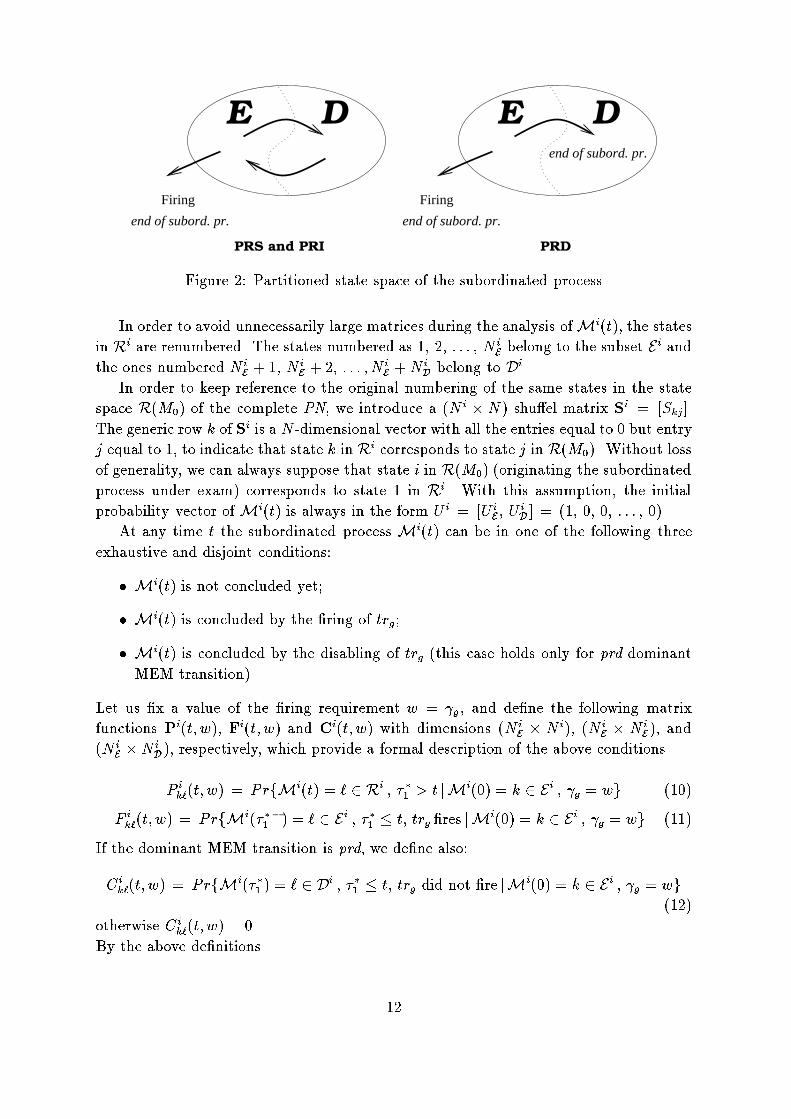
PRS and PRI
E D
Firing
E D
Firing
end of subord. pr. end of subord. pr.
end of subord. pr.
PRD
Figure 2: Partitioned state space of the subordinated process
In order to avoid unnecessarily large matrices during the analysis ofM
i
(t), the states
in R
i
are renumbered. The states numbered as 1; 2; : : : ; N
i
E
belong to the subset E
i
and
the ones numbered N
i
E
+ 1; N
i
E
+ 2; : : : ; N
i
E
+N
i
D
belong to D
i
.
In order to keep reference to the original numbering of the same states in the state
space R(M
0
) of the complete PN, we introduce a (N
i
� N) shu�el matrix S
i
= [S
kj
].
The generic row k of S
i
is a N -dimensional vector with all the entries equal to 0 but entry
j equal to 1, to indicate that state k in R
i
corresponds to state j in R(M
0
). Without loss
of generality, we can always suppose that state i in R(M
0
) (originating the subordinated
process under exam) corresponds to state 1 in R
i
. With this assumption, the initial
probability vector of M
i
(t) is always in the form U
i
= [U
i
E
; U
i
D
] = (1; 0; 0; : : : ; 0).
At any time t the subordinated process M
i
(t) can be in one of the following three
exhaustive and disjoint conditions:
� M
i
(t) is not concluded yet;
� M
i
(t) is concluded by the �ring of tr
g
;
� M
i
(t) is concluded by the disabling of tr
g
(this case holds only for prd dominant
MEM transition).
Let us �x a value of the �ring requirement w =
g
, and de�ne the following matrix
functions P
i
(t; w), F
i
(t; w) and C
i
(t; w) with dimensions (N
i
E
� N
i
), (N
i
E
� N
i
E
), and
(N
i
E
�N
i
D
), respectively, which provide a formal description of the above conditions.
P
i
k`
(t; w) = PrfM
i
(t) = ` 2 R
i
; �
�
1
> t jM
i
(0) = k 2 E
i
;
g
= wg (10)
F
i
k`
(t; w) = PrfM
i
(�
��
1
) = ` 2 E
i
; �
�
1
� t; tr
g
�res jM
i
(0) = k 2 E
i
;
g
= wg (11)
If the dominant MEM transition is prd, we de�ne also:
C
i
k`
(t; w) = PrfM
i
(�
�
1
) = ` 2 D
i
; �
�
1
� t; tr
g
did not �re jM
i
(0) = k 2 E
i
;
g
= wg
(12)
otherwise C
i
k`
(t; w) = 0.
By the above de�nitions
12
� P
i
k`
(t; w) is the probability that M
i
(t) is in state ` 2 R
i
at time t before the age
variable of the dominant transition reaches the value w, starting in state k 2 E
i
at
t = 0.
� F
i
k`
(t; w) is the probability that tr
g
�res from state ` 2 E
i
(the age variable of the
dominant transition reaches the value w in `) before t, starting in state k 2 E
i
at
t = 0.
� C
i
k`
(t; w) with prd dominant MEM transition is the probability that a transition to
` 2 D
i
occurs (resetting a
g
) before the �ring of tr
g
and before time t, starting in
state k 2 E
i
at t = 0.
The conditions covered by Equations (10), (11) and (12), represent all the possible
outcomes of M
i
(t) at a given time t. Hence, for any t � 0 and k 2 E
i
:
X
`2R
i
P
i
k`
(t; w) +
X
`2E
i
F
i
k`
(t; w) +
X
`2D
i
C
i
k`
(t; w) = 1 (13)
Let us further introduce the (N
i
E
�N) branching probability matrix�
i
= [�
i
kj
]. The
generic entry �
i
kj
represents the probability that the �ring of the dominant transition
tr
g
in state k 2 E
i
leads to a marking j 2 R(M
0
).
�
i
kj
= Pr fnext marking is j 2 R(M
0
) j current marking is k 2 E
i
; tr
g
�res g
If immediate transitions are excluded from the original PN de�nition (as in the present
setting), each row of �
i
contains one and only one entry equal to 1 being all the other
entries equal to 0. However, if immediate transitions are allowed, their e�ect could be
accounted for by properly modifying the entries of �
i
[8]. In this case, the probability
of jumping from a tangible state k to any possible tangible state j through vanishing
markings, must be located in the proper �
i
kj
entry of �
i
(being the sum of each row
equal to 1).
Remembering the initial probability vector U
i
of the subordinated processM
i
(t), the
elements of the ith row of matrices K(t) and E(t) can be expressed as a function of the
elements of the �rst row of the matrices P
i
(t; w), F
i
(t; w) and C
i
(t; w) in the following
way:
K
i
(t) =
Z
1
w=0
U
i
E
[F
i
(t; w)�
i
+ C
i
(t; w)S
i
D
] dG
g
(w) (14)
E
i
(t) =
Z
1
w=0
U
i
E
P
i
(t; w)S
i
dG
g
(w) (15)
where the notation A
i
(�) refers to the ith row of matrix A(�), and S
i
D
is the proper
(N
i
D
�N) partition of matrix S
i
.
Equations (14) and (15) show how the local and global kernels can be evaluated
from the knowledge of matrices P
i
(t; w), F
i
(t; w) and C
i
(t; w). In the following section,
the above matrices are derived from the analysis of the subordinated process over the
partitioned state space R
i
= E
i
[ D
i
.
13
4.1 Partitioned state space
In order to simply the notation, in the following derivation we eliminate the superscript
i in all the symbols.
It is however tacitly intended, that all the quantities refer to the single speci�c process
M
i
(t) subordinated to the regeneration period starting from state i.
With reference to Figure 2, and with the adopted renumbering of the states, M
i
(t)
starts in state 1 2 E, then moves through states in D reentering E in any state k 2 E.
However, the dominant transition of M
i
(t) can only �re from states in E. Let us denote
by T
1
the random time point until M
i
(t) visits E and by T
2
the random time point
until M
i
(t) visits D. By enumerating all the possible exhaustive and mutually exclusive
conditions in which the subordinated process M
i
(t) can be in states belonging to E or
D, the following partitioned measures can be evaluated. For states in E we de�ne:
PE
k`
(t; w) = PrfM
i
(t) = ` 2 E ; �
�
1
> t ; T
1
> t jM
i
(0) = k 2 E ;
g
= wg (16)
FE
k`
(t; w) = PrfM
i
(�
�
1
�
) = ` 2 E ; �
�
1
� t ; T
1
> �
�
1
jM
i
(0) = k 2 E ;
g
= wg (17)
PED
k`
(t; w) = PrfM
i
(T
1
) = ` 2 D ; �
�
1
> T
1
; T
1
< t jM
i
(0) = k 2 E ;
g
= wg (18)
Since tr
g
can not �re from D we also de�ne:
PD
k`
(t) = PrfM
i
(t) = ` 2 D ; T
2
> t jM
i
(0) = k 2 Dg (19)
PDE
k`
(t) = PrfM
i
(T
2
) = ` 2 E ; T
2
< t jM
i
(0) = k 2 Dg (20)
By the above de�nitions it follows that:
� PE(t; w) is a (N
E
� N
E
) dimensional matrix whose generic element PE
k`
(t; w) is
the probability of being at time t in state ` 2 E starting in state k 2 E at t = 0,
without intermediate passage to D and before the �ring of the dominant transition.
� FE(t; w) is a (N
E
� N
E
) dimensional matrix whose generic element FE
k`
(t; w) is
the probability that tr
g
�res from state ` 2 E before t, starting in state k 2 E at
t = 0, and without intermediate passage to D.
� PED(t; w) is a (N
E
�N
D
) dimensional matrix whose generic element PED
k`
(t; w)
is the probability that the subordinated process left E before time t and before the
�ring of the dominant transition, hitting state ` 2 D, starting from state k 2 E at
t = 0.
14
� PD(t; w) is a (N
D
�N
D
) dimensional matrix whose generic element PD
k`
(t) is the
probability of being at time t in state ` 2 D starting in state k 2 D at t = 0, and
without intermediate passage to E.
� PDE(t; w) is a (N
D
�N
E
) dimensional matrix whose generic element PDE
k`
(t) is
the probability that the subordinated process left D before time t hitting state
` 2 E, starting in state k 2 D at t = 0.
Given that the process started in a state k 2 E at t = 0, the following equality holds:
X
`2E
PE
k`
(t; w) +
X
`2D
PED
k`
(t; w) +
X
`2E
FE
k`
(t; w) = 1
The process starting from D is very similar to the one starting from E. The only
di�erence between the two is that the �ring of tr
g
is not possible in D. Hence, these
measures are independent of the �ring time requirement (w) and:
X
`2D
PD
k`
(t) +
X
`2E
PDE
k`
(t) = 1
The functions (16) to (20), are de�ned without any speci�c reference to the particular
execution policy of the dominant transition. However, this knowledge is now necessary
to evaluate the matrix functions P(t; w), F(t; w) and C(t; w) from Equation (16) - (20),
and then the kernel matrices of the MRSPN.
4.1.1 prd dominant MEM transition
Any transition out of subset E (either by �ring or by disabling the dominant transition
tr
g
) terminates the subordinated process M
i
(t).
Theorem 2 The time-domain and the LST transform expressions of the probability ma-
trices P(t; w), F(t; w) and C(t; w) satisfy:
P(t; w) = [PE(t; w); 0 ] P
�
(s;w) = [PE
�
(s;w); 0 ]
F(t; w) = FE(t; w) F
�
(s;w) = FE
�
(s;w)
C(t; w) = PED(t; w) C
�
(s;w) = PED
�
(s;w)
(21)
The proof follows directly from the de�nition of the functions [5]. The equality in
the LST domain has been explicitly reported, because this form is derived directly in the
next section.
In the �rst line of (21), P(t; w) = [�
EE
; �
ED
] is expressed in partitioned form, being
the second partition the (N
E
�N
D
) 0 matrix, since under the prd policy no transition is
possible from E to D before the successive RTP.
15
4.1.2 pri type dominant MEM transition
The regeneration period can be concluded only by the �ring of the dominant pri transition
from a state in E. However, the �ring can occur after (0; 1; 2; : : :) visits in D. Any time
the subordinated process enters or re-enters E, an identical �ring time requirement w
has to be completed.
Theorem 3 The LST transform of the probability matrices P(t; w), F(t; w) and C(t; w)
satisfy:
F
�
(s;w) = [I � PED
�
(s;w) PDE
�
(s)]
�1
FE
�
(s;w) (22)
P
�
(s;w) = [I � PED
�
(s;w) PDE
�
(s)]
�1
[PE
�
(s;w); PED
�
(s;w) PD
�
(s)](23)
C
�
(s;w) = 0 (24)
where the second member of the r.h.s. of Equation (23) is expressed in the same parti-
tioned form as in (21).
The proof is given in Appendix A.
4.1.3 prs type dominant MEM transition
The analysis of the process subordinated to a dominant prs transition is very similar to
the pri case, examined in the previous subsection. Also in the prs case, the regeneration
period can be concluded only by the �ring of the dominant transition from a state in
E. The �ring can occur after (0; 1; 2; : : :) visits in D, but any time the subordinated
process enters or re-enters E, only the residual �ring time needs to be accomplished.
Theorem 4 The double transform of the probability matrices P(t; w), F(t; w) and
C(t; w) satisfy:
F
��
(s; v) = [I� vPED
��
(s; v)PDE
�
(s)]
�1
FE
��
(s; v) (25)
P
��
(s; v) = [I� vPED
��
(s; v) PDE
�
(s)]
�1
[PE
��
(s; v) ; PED
��
(s; v) PD
�
(s)](26)
C
��
(s; v) = 0 (27)
where superscript
�
means Laplace transformation, and v is the complex transform vari-
able of w (i.e.: F
�
(v) =
R
1
0
F (w)e
�vw
dw).
The proof of Theorem 4 is given in Appendix B by resorting to a renewal argument.
16
4.2 Subordinated process of speci�c structure
If the stochastic structure of the subordinated process M
i
(t) is known, the measures
derived in the previous sections can be expressed in closed form and solved. In the
following two paragraphs, we consider the particular cases in which the subordinated
process is a SMP or a CTMC.
4.2.1 Subordinated SMP
Let M
i
(t) be a SMP whose probability transition matrix is a (N
i
�N
i
) matrix denoted
by Q(t) = [Q
k`
(t)]. Let the sojourn time distribution of state k be Q
k
(t) =
P
`2R
iQ
k`
(t).
Theorem 5 When the subordinated process is a SMP, the measures de�ned on the par-
titioned state space given in Equations (16) - (20), take the form:
PE
��
k`
(s; v) = �
k`
s [1 � Q
�
k
(s + v) ]
v(s + v)
+
X
u2E
Q
�
ku
(s + v)PE
��
u`
(s; v); k; ` 2 E (28)
FE
��
k`
(s; v) = �
k`
1 � Q
�
k
(s + v)
s + v
+
X
u2E
Q
�
ku
(s + v)FE
��
u`
(s; v); k; ` 2 E (29)
PED
��
k`
(s; v) =
1
v
Q
�
k`
(s + v) +
X
u2E
Q
�
ku
(s + v)PED
��
u`
(s; v); k 2 E; ` 2 D (30)
PD
�
k`
(s) = �
k`
[1 �Q
�
k
(s)] +
X
u2D
Q
�
ku
(s) PD
�
u`
(s); k; ` 2 D
(31)
PDE
�
k`
(s) = Q
�
k`
(s) +
X
u2D
Q
�
ku
(s)PDE
�
u`
(s); k 2 D; ` 2 E (32)
The proof of Theorem 5 can be found in Appendix C.
The Equations (28) - (32) must be substituted in the expressions for the matrices
P(t; w), F(t; w) and C(t; w) given in Theorems 2 - 4. Then Equation (14) and (15) can
be applied. Further symbolical manipulation requires the knowledge of the particular
functions in Q(t).
4.2.2 Subordinated CTMC
Let M
i
(t) be a CTMC whose in�nitesimal generator is a (N
i
�N
i
) matrix denoted by
A = [a
k`
]. The in�nitesimal generator can be expressed in the following partitioned
form:
17

A =
N
E
N
D
N
E
A
E
A
ED
N
D
A
DE
A
D
(33)
With respect to the SMP case, considered in the previous section, the following corre-
spondence can be established:
Q
�
k`
(s) =
8
>
>
<
>
>
:
a
k`
s � a
kk
if : k 6= `
0 if : k = `
(34)
where a
kk
= �
P
`2R
i
; ` 6=k
a
k`
. Applying a direct substitution of (34) into (28) - (32), the
partitioned measures can be expressed in matrix form based on the block description
(33) of the in�nitesimal generator of the subordinated CTMC [5, 3]. The matrix form is
given in the LST domain, being, as usual, s the transform variable of the time t and v
the transform variable of the sampled �ring time w.
PE
��
(s; v) =
s
v
((s+ v)I � A
E
)
�1
(35)
FE
��
(s; v) = ((s+ v)I � A
E
)
�1
(36)
PED
��
(s; v) =
1
v
((s+ v)I � A
E
)
�1
A
ED
(37)
PD
�
(s) = s (sI � A
D
)
�1
(38)
PDE
�
(s) = (sI � A
D
)
�1
A
DE
(39)
After a symbolical inverse Laplace transformation according to the variable v, Equa-
tions (35), (36) and (37) become, respectively:
PE
�
(s;w) = s
Z
w
0
e
(�sI+A
E
)z
dz (40)
FE
�
(s;w) = e
(�sI+A
E
)w
(41)
PED
�
(s;w) =
Z
w
0
e
(�sI+A
E
)z
dz A
ED
(42)
18

5 Steady state analysis
The steady-state analysis is based on Equations (6) and (7) of Section 3.1. In general, the
transient analysis of the kernel elements is needed, so that the computational complexity
of the steady-state solution is the same as the one of the transient solution.
However, if the subordinated process is a CTMC, Equations (6) and (7) can be solved
explicitly, and the elements of the matrices � and � can be expressed directly from the
in�nitesimal generator A. Hence, in this case, the steady-state solution can be obtained
by a computationally e�ective method. The proper expressions when the dominant
transition is either prd or prs or pri are presented in the following subsections.
Let us now concentrate on the steady-state analysis of a single subordinated process
M
i
(t) starting from state i 2 R
TP
(M
0
) under the hypothesis that M
i
(t) is a CTMC
with in�nitesimal generator of the form (33). Combining Equations (6) and (7) with
Equations (15) and (14), the ith row of matrices � and � can be written as:
�
i
= lim
s!0
1
s
E
�
i
(s) = lim
s!0
Z
1
w=0
U
i
E
1
s
P
i�
(s;w)S
i
dG
g
(w) (43)
�
i
= lim
s!0
K
�
i
(s) = lim
s!0
Z
1
w=0
U
i
E
[F
i�
(s;w)�
i
+ C
i�
(s;w)S
i
D
] dG
g
(w) (44)
If the dominant transition is deterministic, Equations (43) and (44) simplify, since
the integration
R
1
w=0
[�] dG
g
(w) is avoided. Equations (43) and (44) are now particular-
ized according to the preemption policy of the dominant transition. In the sequel, the
superscript i in the symbols is omitted.
5.1 The dominant MEM transition is prd
Theorem 6 Given the dominant transition is prd, and the subordinated process is a
CTMC with generator of the form (33), the �
i
and �
i
row vectors are given by:
�
i
=
Z
1
w=0
U
E
[L(w); 0 ] S dG
g
(w) (45)
�
i
=
Z
1
w=0
U
E
[ e
wA
E
� + L(w) A
ED
S
D
] dG
g
(w) (46)
where L(w) =
Z
w
z=0
e
zA
E
dz.
Proof - From (21) and (40) we obtain:
lim
s!0
1
s
P
�
(s;w) = lim
s!0
1
s
[PE
�
(s;w); 0 ] = [L(w); 0 ] (47)
substituting (47) into (43), Equation (45) is obtained. Furthermore, from (21), (41) and
(42), we get:
lim
s!0
[F
�
(s;w)� + C
�
(s;w)S
D
] = lim
s!0
[FE
�
(s;w)� + PED
�
(s;w) S
D
] =
FE
�
(0; w)� + PED
�
(0; w) S
D
= e
wA
E
� + L(w) A
ED
S
D
(48)
19
Equation (48), combined with (44), provides (46) 2.
Theorem 6 shows that the row elements of matrices � and � can be directly evaluated
from the in�nitesimal generator of the underlying CTMC at the same cost of evaluating
the transient solution (term e
wA
E
in Equation 46), or the integral solution (term L(w)
in Equations 45 and 46), up to time w.
5.2 The dominant MEM transition is pri
Theorem 7 Given the dominant transition is pri, and the subordinated process is a
CTMC with generator of the form (33), the �
i
and �
i
row vectors are given by:
�
i
=
Z
1
w=0
U
E
[ I + L(w)A
ED
A
�1
D
A
DE
]
�1
[L(w); �L(w)A
ED
A
�1
D
] S dG
g
(w)(49)
�
i
=
Z
1
w=0
U
E
[ I + L(w)A
ED
A
�1
D
A
DE
]
�1
e
wA
E
� dG
g
(w) (50)
where L(w) =
Z
w
z=0
e
zA
E
dz.
Proof - From (23), we obtain:
lim
s!0
1
s
P
�
(s;w) =
lim
s!0
1
s
[I � PED
�
(s;w) PDE
�
(s)]
�1
[PE
�
(s;w); PED
�
(s;w) PD
�
(s)]
(51)
remembering the explicit expressions from (35) to (42), expression (49) is easily obtained.
Similarly, from (22), we have:
lim
s!0
F
�
(s;w) = [I � PED
�
(s;w) PDE
�
(s)]
�1
FE
�
(s;w) (52)
from which Equation (50) can be obtained by substituting the explicit expressions (35)
- (42) in the corresponding terms in (52). 2
The steady-state solution in the pri case, involves the inversion of matrix A
D
and of
the matrix term I + L(w)A
ED
A
�1
D
A
DE
. The cardinality of these square matrices is
equal to the number of states in D and E, respectively. However, all the terms can be
computed by the knowledge of the in�nitesimal generator of the subordinated CTMC,
only.
5.3 The dominant MEM transition is prs
Theorem 8 Given the dominant transition is prs, and the subordinated process is a
CTMC with generator of the form (33), the �
i
and �
i
row vectors are given by:
�
i
=
Z
1
w=0
U
E
h
L
�
(w) ; �L
�
(w) A
ED
A
�1
D
i
dG
g
(w) (53)
�
i
=
Z
1
w=0
U
E
[ e
w�
]� dG
g
(w) (54)
20

where
� = A
E
� A
ED
A
�1
D
A
ED
and L
�
(w) =
Z
w
z=0
e
z�
dz
Proof - We adopt the notation LT
�1
v!w
A
�
(v) = A(w) to indicate the inverse Laplace
transformation with respect to the variable v. From (26) and (35) - (42), by successive
manipulations, we can write:
LT
�1
v!w
lim
s!0
1
s
P
��
(s; v)
= LT
�1
v!w
lim
s!0
1
s
[I � vPED
��
(s; v) PDE
�
(s)]
�1
[PE
��
(s; v) ; PED
��
(s; v) PD
�
(s)]
= LT
�1
v!w
[ I+ (vI�A
E
)
�1
A
ED
A
�1
D
A
DE
]
�1
[
1
v
(vI�A
E
)
�1
; �
1
v
(vI�A
E
)
�1
A
ED
A
�1
D
]
= LT
�1
v!w
[
1
v
(vI� �)
�1
; �(vI�
1
v
�)
�1
A
ED
A
�1
D
]
(55)
from which Equation (53) is obtained. Furthermore, from (25), we can write:
LT
�1
v!w
[ lim
s!0
F
��
(s; v) ]
= LT
�1
v!w
[ I+ (vI�A
E
)
�1
A
ED
A
�1
D
A
DE
]
�1
(vI�A
E
)
�1
= LT
�1
v!w
[ (vI� �)
�1
]
(56)
Equation (54) comes from (56). 2
Matrix � is the in�nitesimal generator of a CTMC de�ned over the states in E.
Hence, the computational complexity associated to the solution of Equations (53) and
(54) is determined by the computation of � (that involves the inverse of A
D
), and the
evaluation of the transient solution of the CTMC with generator � up to time w (terms
[e
w�
]) and its integral (term [L
�
(w)]). A fully developed example has been reported in
[31].
6 Combined preemption policies: an example
A two processor system runs two types of jobs according to the following scheduling
policy. Jobs of class 1 require both processors and have preemptive priority over jobs of
class 2. Jobs of class 2 have lower priority and are scheduled to run on a single processor
that is chosen according to a prede�ned switching probability.
A PN modeling the system operation according to the described scheduling policy
is represented in Figure 3a. Place p
1
is the customer of class 2 thinking. The thinking
time is exponentially distributed with a global rate �. However, with a rate c � � jobs
are directed to processor 1 (transition t
1
), and with a rate (1� c) �� jobs are directed to
21

��
��
��
��
r
��
��
��
��
?
6
s
0
s
2
t
5
t
6
10010
10001
a) b)
p
1
��
��
��
��
66
��
��
r
p
4
�
�/
S
Sw�
�7
S
So
c c
T
T
T
T
T
T
T
T
�
�
�
�
�
�
�
�
p
5
p
2
p
3
t
4
t
2
t
5
t
6
��
��
��
��
?
6
s
3
s
5
t
5
t
6
00110
00101
��
��
��
��
?
6
s
1
s
4
t
5
t
6
01010
01001
t
3
t
1
t
3
t
2
t
4
t
1
-
��
-
� -
(pri)(prs)
S
S
S
S
S
So
�
�
�
�
�
�7
t
1
�
�
�
��
C
C
C
CW
�
�
��
C
C
CW
t
3
Figure 3: The Petri net and the reachability graph of the two processor system
processor 2 (transition t
3
). Place p
2
(p
3
) is processor 1 (processor 2) serving customer
2 with service time distribution modeled by transition t
2
(t
4
). Place p
4
is customer 1
thinking, while place p
5
represents jobs of class 1 running on both processors while pre-
empting customer 2 under service. (Inhibitor arcs from p
5
to both t
2
and t
4
). Transitions
t
5
and t
6
represent the arrival and the service of jobs of class 1 and have an exponentially
distributed �ring time with parameter �
5
and �
6
, respectively.
We assume that the service time of customer 2 is generally distributed. Therefore,
t
2
and t
4
are MEM transitions (�lled rectangles) with distribution G
2
(t) and G
4
(t),
respectively. We further assume that processor 1 has 'state saving' capabilities so that
the execution of jobs is prs. Processor 2, instead, does not have 'state saving' capabilities
so that a recovery of an interrupted job occurs according to a pri policy. To this end, we
associate to transition t
2
a prs policy, and to transition t
4
a pri policy.
Inspection of the reachability graph, depicted in Figure 3b, leads to the following
assertions:
- The instants of entrance into state s
0
and s
2
are always RTPs, and the associ-
ated subordinated processes are concluded by the next state transition due to the
enabled EXP transitions;
- The instants of entrance into states s
1
and s
3
from s
0
are RTPs as well. According
to the described system characteristics the subordinated process starting from state
s
1
(s
3
) is dominated by t
2
(t
4
) with prs (pri) policy and is concluded by the �ring
of t
2
(t
4
), only.
- The instants of entrance into states s
4
and s
5
from s
2
are RTPs. But when states
s
4
and s
5
are entered from s
1
and s
3
they do not generate RTPs since the memory
22
variable associated to transitions t
2
and t
4
, respectively, is never zero. The outgoing
transitions from s
4
and s
5
are EXP transitions.
From the above assertions follows that all the states can become a regeneration state,
i.e. R
TP
(M
0
) = R(M
0
) and N
0
= N = 6. The analysis proceeds by examining in
isolation all the subordinated processes starting from each possible regeneration state.
Subordinated process starting from s
0
- From s
0
, all the enabled transitions are EXP
and the next regeneration marking can be either s
1
, s
2
or s
3
. The subordinated
process is a single step CTMC.
Subordinated process starting from s
2
- From s
2
, all the enabled transitions are EXP
and the next regeneration marking can be s
0
, s
4
or s
5
. The subordinated process
is a single step CTMC.
Subordinated process starting from s
4
- The EXP transition t
6
is the only enabled one,
and the next regeneration marking is s
1
. The subordinated process is a single step
CTMC.
Subordinated process starting from s
5
- The EXP transition t
6
is the only enabled one,
and the next regeneration marking is s
3
. The subordinated process is a single step
CTMC.
Subordinated process starting from s
1
- The subordinated process starting from s
1
is
dominated by the MEM transition t
2
with associated prs policy and is a CTMC
with state space R
s
1
= fs
1
; s
4
g. The next regeneration marking can be s
0
, only.
Subordinated process starting from s
3
- The subordinated process starting from s
3
is
dominated by the MEM transition t
4
with associated pri policy and is a CTMC
with state space R
s
3
= fs
3
; s
5
g. The next regeneration marking can be s
0
, only.
Based on the above considerations, the subordinated processes starting from states
s
0
, s
2
, s
4
and s
5
can be evaluated by simple Markovian analysis, and the corresponding
rows of the kernel matrices in the transient and the steady-state case can be �lled in
based on the knowledge of the transition rates of the enabled exponential transitions.
The analysis of the subordinated processes starting from states s
1
and s
3
deserves a more
detailed description.
6.1 The analysis of the subordinated process starting from s
1
The markings reachable during the subordinated process starting from state s
1
are gen-
erated (Theorem 1) by removing the dominant MEM transition t
2
from the original PN,
and by assuming s
1
as initial marking. Figure 4 shows the reduced PN and its reacha-
bility graph corresponding to the state space R
s
1
of the subordinated process dominated
by the removed transition t
2
. According to the de�nitions of Section 4, the state space
is R
s
1
= fs
1
; s
4
g, where E
s
1
= fs
1
g and D
s
1
= fs
4
g (N
s
1
E
= 1 and N
s
1
D
= 1).
23
��
��
��
��
r
a) b)
p
1
��
��
��
��
6
��
��
r
p
4
�
�/
S
Sw�
�7
S
So
c
T
T
T
T
T
T
T
T
p
5
p
2
p
3
t
4
t
5
t
6
��
��
��
��
?
6
s
1
s
4
t
5
t
6
01010
01001
(pri)
S
S
S
S
S
So
t
1
�
�
�
��
C
C
C
CW
�
�
��
C
C
CW
t
3
E
D
Figure 4: The subordinated process starting from s
1
Since only EXP transitions are enabled in this reduced PN, the subordinated process
is a CTMC with generator
A
s
1
=
"
��
5
�
5
�
6
��
6
#
the non-overlapping condition with subordinated SMP as it is discussed, for example, in
[5, 30]. In this example we assume t
6
to be EXP in order to apply the results available
for the steady state analysis (Equation (45) - (56)).
During the generation of the reachable markings in the subordinated process the
shu�el matrix can be generated based on the correspondence of the states:
S
s
1
=
"
0 1 0 0 0 0
0 0 0 0 1 0
#
;
and the e�ect of the �ring of t
2
is stored as:
�
s
1
=
h
1 0 0 0 0 0
i
:
Applying Equations (35) - (39) for this example, we obtain the following (1 � 1)
matrices:
PE
s
1
��
(s; v) =
s
v(s+ v + �
5
)
FE
s
1
��
(s; v) =
1
s+ v + �
5
PED
s
1
��
(s; v) =
�
5
v(s+ v + �
5
)
24

PD
s
1
�
(s) =
s
s+ �
6
PDE
s
1
�
(s) =
�
6
s+ �
6
Applying Equation (25) and (26), we obtain:
P
s
1
��
(s; v) =
"
s(s+ �
6
)
v[s
2
+ (�
5
+ �
6
)s+ (�
6
+ s)v]
;
s�
5
v[s
2
+ (�
5
+ �
6
)s+ (�
6
+ s)v]
#
F
s
1
��
(s; v) =
s+ �
6
s
2
+ (�
5
+ �
6
)s+ (�
6
+ s)v
An inverse Laplace transformation provides:
P
s
1
�
(s;w) =
�
s+ �
6
�
5
+ �
6
+ s
�
1 � e
�c
1
w
�
;
�
5
�
5
+ �
6
+ s
�
1� e
�c
1
w
�
�
F
s
1
�
(s;w) = e
�c
1
w
where c
1
=
s(�
5
+ �
6
+ s)
�
6
+ s
. Note that condition (13), which is also valid in LST domain,
holds. The next step, which is the application of (14) and (15), results in the 2nd row
of the kernel matrices. To go further in the analytical derivation, let assume that the
service time of customer 2 on processor 1 is uniformly distributed on the interval (x
1
; x
2
).
The cumulative distribution function F (x), its derivative f(x) and the Laplace transform
F
�
(s) are:
F (x) =
8
>
<
>
:
0 0 � x < x
1
x�x
1
x
2
�x
1
x
1
� x � x
2
1 x > x
2
; f(x) =
1
x
2
� x
1
; F
�
(s) =
e
�x
1
s
� e
�x
2
s
s(x
2
� x
1
)
The following expressions hold:
E
�
s
1
s
1
(s) =
s+ �
6
�
5
+ �
6
+ s
"
1�
e
�c
1
x
1
� e
�c
1
x
2
c
1
(x
2
� x
1
)
#
E
�
s
1
s
4
(s) =
�
5
�
5
+ �
6
+ s
"
1�
e
�c
1
x
1
� e
�c
1
x
2
c
1
(x
2
� x
1
)
#
K
�
s
1
s
0
(s) =
e
�c
1
x
1
� e
�c
1
x
2
c
1
(x
2
� x
1
)
To evaluate �
s
1
s
1
and �
s
1
s
4
, Equation (55) is used:
�
s
1
s
1
=
Z
1
0
w dG
2
(w) =
x
1
+ x
2
2
�
s
1
s
4
=
Z
1
0
�
5
�
6
w dG
2
(w) =
�
5
(x
1
+ x
2
)
2�
6
While the 2nd row of the � matrix is know from the fact that next regeneration
period starts always from s
1
.
25

6.2 The analysis of the subordinated process starting from s
3
Following the same approach, one can observe that the subordinated processes starting
from marking s
1
and s
3
are the same two-state CTMC with rates �
5
and �
6
, i.e. A
s
1
=
A
s
3
. Hence, also the partitioned state space related measures (35) - (39) are the same.
The di�erence between the relevant rows of the kernel matrices comes from the di�erent
preemption policies of t
4
(pri) with respect to t
2
(prs).
In order to analyze the subordinated process of a pri dominant transition we also
need (from Equation (40) - (42)):
PE
s
3
�
(s;w) = s
Z
w
0
e
�(s+�
5
)z
dz =
s
s+ �
5
h
1 � e
�(s+�
5
)w
i
FE
s
3
�
(s;w) = e
�(s+�
5
)w
PED
s
3
�
(s;w) = �
5
Z
w
0
e
�(s+�
5
)z
dz =
�
5
s+ �
5
h
1� e
�(s+�
5
)w
i
from which Theorem 3 gives:
P
s
3
�
(s;w) =
"
s(s+ �
6
)(1� c
2
)
(s+ �
5
)(s+ �
6
)� �
5
�
6
(1� c
2
)
;
s�
5
(1 � c
2
)
(s+ �
5
)(s+ �
6
)� �
5
�
6
(1 � c
2
)
#
F
s
3
�
(s;w) =
(s+ �
5
)(s+ �
6
)c
2
(s+ �
5
)(s+ �
6
)� �
5
�
6
(1 � c
2
)
where c
2
= e
�(s+�
5
)w
. Once again, condition (13) holds.
From the above expressions, the 4th row of the kernel matrices E
�
s
3
s
3
(s), E
�
s
3
s
5
(s),
K
�
s
3
s
0
(s) can be obtained by unconditioning with respect to the �ring time distribution
of t
4
.
Considering again the special case when the service time of customer 2 on processor
2 is uniformly distributed on the interval (x
3
; x
4
), we obtain:
E
�
s
3
s
3
(s) =
s+ �
6
s+ �
5
+ �
6
"
(s+ �
6
)c
3
(x
4
� x
3
)�
5
�
6
+ 1
#
E
�
s
3
s
5
(s) =
�
5
s+ �
5
+ �
6
"
(s+ �
6
)c
3
(x
4
� x
3
)�
5
�
6
+ 1
#
K
�
s
3
s
0
(s) = �
(s+ �
6
)c
3
(x
4
� x
3
)�
5
�
6
where c
3
= ln[s(s+ �
5
+ �
6
) + �
5
�
6
e
�(s+�
5
)x
4
]� ln[s(s+ �
5
+ �
6
) + �
5
�
6
e
�(s+�
5
)x
3
].
To compute �
s
3
s
3
and �
s
3
s
5
(49) is used, while �
s
3
s
0
= 1.
�
s
3
s
3
=
Z
1
0
1
�
5
(e
�
5
w
� 1) dG
4
(w) =
1
�
5
"
e
�
5
x
4
� e
�
5
x
3
�
5
(x
4
� x
3
)
� 1
#
�
s
3
s
5
=
Z
1
0
1
�
6
(e
�
5
w
� 1) dG
4
(w) =
1
�
6
"
e
�
5
x
4
� e
�
5
x
3
�
5
(x
4
� x
3
)
� 1
#
26
6.3 Numerical results
The transient analysis can be performed by applying Equation (4), where the complete
kernel matrices are given by:
K
�
(s) =
2
6
6
6
6
6
6
6
6
6
6
6
6
4
0
c �
s+ �+ �
5
�
5
s + �+ �
5
(1� c) �
s+ �+ �
5
0 0
K
�
s
1
s
0
(s) 0 0 0 0 0
�
6
s + �+ �
6
0 0 0
c �
s + �+ �
6
(1� c) �
s+ �+ �
6
K
�
s
3
s
0
(s) 0 0 0 0 0
0
�
6
s+ �
6
0 0 0 0
0 0 0
�
6
s+ �
6
0 0
3
7
7
7
7
7
7
7
7
7
7
7
7
5
E
�
(s) =
2
6
6
6
6
6
6
6
6
6
6
6
6
6
4
s
s + � + �
5
0 0 0 0 0
0 E
�
s
1
s
1
(s) 0 0 E
�
s
1
s
4
(s) 0
0 0
s
s + � + �
6
0 0 0
0 0 0 E
�
s
3
s
3
(s) 0 E
�
s
3
s
5
(s)
0 0 0 0
s
s + �
6
0
0 0 0 0 0
s
s+ �
6
3
7
7
7
7
7
7
7
7
7
7
7
7
7
5
The steady state analysis requires the computation of the following matrices:
� =
2
6
6
6
6
6
6
6
6
6
6
6
6
4
0
c �
�+ �
5
�
5
�+ �
5
(1� c) �
� + �
5
0 0
1 0 0 0 0 0
�
6
� + �
6
0 0 0
c �
� + �
6
(1� c) �
�+ �
6
1 0 0 0 0 0
0 1 0 0 0 0
0 0 0 1 0 0
3
7
7
7
7
7
7
7
7
7
7
7
7
5
� =
2
6
6
6
6
6
6
6
6
6
6
6
6
6
6
4
1
� + �
5
0 0 0 0 0
0 �
s
1
s
1
0 0 �
s
1
s
4
0
0 0
1
� + �
6
0 0 0
0 0 0 �
s
3
s
3
0 �
s
3
s
5
0 0 0 0
1
�
6
0
0 0 0 0 0
1
�
6
3
7
7
7
7
7
7
7
7
7
7
7
7
7
7
5
Suppose that the two processors are of di�erent classes, and the average computation
time on processor 1 is less than on processor 2 (i.e.: x
2
� x
1
> x
4
� x
3
). The considered
design problem consists in optimizing the switching probability c in order to optimize
the performance characteristics of the system.
The steady state probabilities (v
j
) can be evaluated based on � and � by Equation
(8) and (9). With a given tra�c pattern the dependence of the system performance on
27

00.2
0.40.6
0.81
c
1
2
3
la5
0
0.2
0.4
0.6
0.8
Pr
00.2
0.40.6
0.81
c
1
2
3
la5
0
0.2
.4
.6
8
Figure 5: Probability of state s
0
(idle state) versus c and �
5
0 0.20.40.60.8 1
0.5
1
1.5
2
2.5
3
Figure 6: Surface plot of Figure 5
c can be measured by the steady state probability of the idle state (s
0
). The better the
system performance is, the higher is the steady state probability of s
0
.
In Figure 5, the steady state probability of s
0
is depicted as a function of the switching
probability (c) and the submission rate of customer 1 (�
5
). Figure 5 contains the 3D-view
of the function. In order to emphasize the dependence on c Figure 6 shows the surface
plot of it. The parameters of the model are set as follows:
� the submission rate of customer 1 (�
5
) is varying from 0:1 to 3,
� the service rate of customer 1 (�
6
) is 1,
� the submission rate of customer 2 (�) is 0:2,
� the service time of customer 2 is assumed to be uniformly distributed. On the slower
processor (processor 1) the service time (�ring time of t
2
) is uniformly distributed
on (0; 2) (i.e.: x
1
= 0; x
2
= 2), while on the faster processor (processor 2) the service
time (�ring time of t
4
) is uniformly distributed on (0; 1) (i.e.: x
3
= 0; x
4
= 1),
28
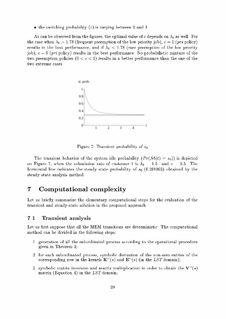
� the switching probability (c) is varying between 0 and 1.
As can be observed from the �gures, the optimal value of c depends on �
5
as well. For
the case when �
5
> 1:78 (frequent preemption of the low priority job), c = 1 (prs policy)
results in the best performance, and if �
5
< 1:78 (rare preemption of the low priority
job), c = 0 (pri policy) results in the best performance. No probabilistic mixture of the
two preemption policies (0 < c < 1) results in a better performance than the one of the
two extreme cases.
1 2 3 4t0
0.2
0.4
0.6
0.8
1
st. prob.
Figure 7: Transient probability of s
0
The transient behavior of the system idle probability (Pr(M(t) = s
0
)) is depicted
on Figure 7, when the submission rate of customer 1 is �
5
= 1:5. and c = 0:5. The
horizontal line indicates the steady state probability of s
0
(0:281063) obtained by the
steady state analysis method.
7 Computational complexity
Let us brie y summarize the elementary computational steps for the evaluation of the
transient and steady-state solution in the proposed approach.
7.1 Transient analysis
Let us �rst suppose that all the MEM transitions are deterministic. The computational
method can be divided in the following steps:
1. generation of all the subordinated process according to the operational procedure
given in Theorem 1;
2. for each subordinated process, symbolic derivation of the non-zero entries of the
corresponding row in the kernels K
�
(s) and E
�
(s) (in the LST domain);
3. symbolic matrix inversion and matrix multiplication in order to obtain the V
�
(s)
matrix (Equation 4) in the LST domain;
29
4. time domain solution obtained by a numerical inversion of the entries of the V
�
(s).
If the dominant MEM transition is not deterministic, Step 2) in the above list should
be replaced by:
2
0
symbolic derivation of the entries of the K
�
(s) and E
�
(s) matrices in LST domain
as in the deterministic case;
2
00
unconditioning of the entries of the K
�
(s) and E
�
(s) matrices, according to the
Cdf of the �ring time of the MEM transitions (Equations (14) and (15)).
Any standard algorithm generating reachability graph from standard PN description
can be used for Step 1); during the generation of the state space of a given subordinated
process, matrices � and S must be �lled in. In our case Step 2) is done manually, only
because of the intrinsic limitations of the mathematical packages we used in manipulating
symbolic algebraic expressions. The complexity of this step depends on the non-zero
entries of the involved matrices, and on the complexity of the process subordinated to
the dominant MEM transitions.
The computational complexity of Step 3) depends on the dimension of the matri-
ces (i.e. the number of tangible markings) and the complexity of the elements of the
kernels (the di�culty of Step 3 is related to the di�culty of Step 2). We performed
these symbolic computations using MATHEMATICA. The complexity of the numerical
inversion at Step 4) also depends on two factors; the complexity of the function to in-
vert, and the prescribed accuracy. We used the Jagerman's method [21] implemented in
MATHEMATICA language.
7.2 Steady-state analysis
In the general case the steady-state analysis follows the same procedure described for
the transient one. However, a very e�cient technique has been extensively discussed in
Section 5 in the particular case where all the subordinated processes are CTMCs. The
main di�erence is that the introduced method is composed by numerical analysis steps
only, hence it does not require any symbolic and transform domain manipulation as it is
in the case of transient analysis.
If the transition dominating the considered regeneration period is deterministic, the
steady-state analysis requires for each subordinated process the transient solution for
the instantaneous and integral probabilities of a CTMC up to the �ring time w of the
dominant transition. Any standard algorithm can be used at this purpose, and it is known
that the computation of the instantaneous probabilities and of the integral probabilities
can be performed at the same time with a very little overhead [28, 29]. When the
transition dominating the considered regeneration period is not deterministic, numerical
integration according to the distribution of the �ring time has to be performed [26].
30
8 Conclusion
The paper has provided a detailed discussion and an analytical procedure to deal with the
class ofMRSPN with non-overlapping dominant transitions. The analytical description is
based on the Markov renewal theory and allows to include di�erent preemption policies
associated to di�erent dominant transitions into a single MRSPN model. Complete
analytical descriptions have been provided for the transient and steady state cases, when
all the subordinated processes are restricted to be CTMC or SMP.
The complexity of the proposed approach has been discussed and, for the steady-
state analysis with subordinated CTMCs, a procedure ready to be implemented into an
automatic solution tool has been provided.
The transient analysis still requires some symbolic manipulation. However, we believe
that all the necessary elements for its automatic computation have been fully identi�ed.
Our approach extends previously available results and o�er the possibility to adopt
di�erent preemption policies inside the same model, thus widening the �eld of applica-
bility of stochastic Petri nets.
Future extensions are related with the introduction of interlaced, or state dependent,
memory policies, where the memory of a transition can be modi�ed by the occurrence
of some condition on the net.
Acknowledgements
This work has been partially supported by the Italian CNR under Grant No. 96-01939-
CT12 and the Hungarian OTKA under Grant No. T-16637.
References
[1] M. Ajmone Marsan, G. Balbo, A. Bobbio, G. Chiola, G. Conte, and A. Cumani.
The e�ect of execution policies on the semantics and analysis of stochastic Petri
nets. IEEE Transactions on Software Engineering, SE-15:832{846, 1989.
[2] M. Ajmone Marsan and G. Chiola. On Petri nets with deterministic and exponen-
tially distributed �ring times. In Lecture Notes in Computer Science, volume 266,
pages 132{145. Springer Verlag, 1987.
[3] A. Bobbio, V.G. Kulkarni, A. Pulia�to, M. Telek, and K. Trivedi. Preemptive
repeat identical transitions in Markov Regenerative Stochastic Petri Nets. In 6-th
International Conference on Petri Nets and Performance Models - PNPM95, pages
113{122. IEEE Computer Society, 1995.
[4] A. Bobbio and M. Telek. Combined preemption policies in MRSPN. In Ravi Mittal
et al., editor, Fault Tolerant Systems and Software, pages 92{98. Narosa Pub. House,
New Dehli - India, 1995.
31
[5] A. Bobbio and M. Telek. Markov regenerative SPN with non-overlapping activity
cycles. In International Computer Performance and Dependability Symposium -
IPDS95, pages 124{133. IEEE Computer Society Press, 1995.
[6] A. Bobbio and M. Telek. Non-exponential stochastic Petri nets: an overview of
methods and techniques. In To be published in: Computer Systems Science & En-
gineering, 1997.
[7] Hoon Choi, V.G. Kulkarni, and K. Trivedi. Transient analysis of deterministic
and stochastic Petri nets. In Proceedings of the 14-th International Conference on
Application and Theory of Petri Nets, Chicago, June 1993.
[8] Hoon Choi, V.G. Kulkarni, and K. Trivedi. Markov regenerative stochastic Petri
nets. Performance Evaluation, 20:337{357, 1994.
[9] G. Ciardo. Discrete-time markovian stochastic Petri nets. In Proceedings of the 2-nd
International Workshop on Numerical Solution of Markov Chains, pages 339{358,
1995.
[10] G. Ciardo, R. German, and C. Lindemann. A characterization of the stochastic pro-
cess underlying a stochastic Petri net. IEEE Transactions on Software Engineering,
20:506{515, 1994.
[11] G. Ciardo and K.S. Trivedi. A decomposition approach for stochastic reward net
models. Performance Evaluation, 18:37{59, 1993.
[12] G. Ciardo and R. Zijal. Well-de�ned stochastic Petri nets. In Proceedings of the
4-th International Workshop on Modeling Analysis and Simulation of Computer
and Telecommunication Systems (MASCOTS'96), pages 278{284. IEEE Computer
Society Press, 1996.
[13] E. Cinlar. Introduction to Stochastic Processes. Prentice-Hall, Englewood Cli�s,
1975.
[14] A. Cumani. Esp - A package for the evaluation of stochastic Petri nets with phase-
type distributed transition times. In Proceedings International Workshop Timed
Petri Nets, pages 144{151, Torino (Italy), 1985. IEEE Computer Society Press no.
674.
[15] J. Bechta Dugan, K. Trivedi, R. Geist, and V.F. Nicola. Extended stochastic Petri
nets: applications and analysis. In Proceedings PERFORMANCE '84, Paris, 1984.
[16] R. German. Transient Analysis of deterministic and stochastic Petri nets by the
method of supplementary variables. MASCOT'95, 1995.
[17] R. German, D. Logothetis, and K. Trivedi. Transient analysis of Markov Regenera-
tive Stochastic Petri Nets: a comparison of approaches. In 6-th International Con-
ference on Petri Nets and Performance Models - PNPM95, pages 103{112. IEEE
Computer Society, 1995.
[18] P.J. Haas and G.S. Shedler. Regenerative stochastic Petri nets. Performance Eval-
uation, 6:189{204, 1986.
[19] B.R. Haverkort and K. Trivedi. Speci�cation techniques for Markov Reward Models.
Discrete Event Dynamic Systems: Theory and Applications, 3:219{247, 1993.
32
[20] M.A. Holliday and M.K. Vernon. A generalized timed Petri net model for per-
formance analysis. IEEE Transactions on Software Engineering, SE-13:1297{1310,
1987.
[21] D.L. Jagerman. An inversion technique for the Laplace transform. The Bell System
Technical Journal, 61:1995{2002, October 1982.
[22] V.G. Kulkarni. Modeling and Analysis of Stochastic Systems. Chapman Hall, 1995.
[23] C. Lindemann. An improved numerical algorithm for calculating steady-state so-
lutions of deterministic and stochastic Petri net models. Performance Evaluation,
18:75{95, 1993.
[24] C. Lindemann. DSPNexpress: a software package for the e�cient solution of deter-
ministic and stochastic Petri nets. Performance Evaluation, 22:3{21, 1995.
[25] M.K. Molloy. Discrete time stochastic Petri nets. IEEE Transactions on Software
Engineering, SE-11:417{423, 1985.
[26] W.H. Press, S.A. Teukolsky, W.T. Vetterling and B.P. Flannery. Numerical Recipes
in C: The art of Scienti�c Computing. Cambridge University Press, 1992.
[27] A. Pulia�to, M. Scarpa, and K.S. Trivedi. Petri nets with k simultaneously enabled
generally distributed timed transitions. In To appear in: Performance Evaluation,
1997.
[28] A. Reibman and K.S. Trivedi. Numerical transient analysis of Markov models.
Computers and Operations Research, 15:19{36, 1988.
[29] A. Reibman and K.S. Trivedi. Transient analysis of cumulative measures of Markov
chain behavior. Stochastic Models, 5:683{710, 1989.
[30] M. Telek and A. Bobbio. Markov regenerative stochastic Petri nets with age type
general transitions. In G. De Michelis and M. Diaz, editors, Application and Theory
of Petri Nets (16-th International Conference), Lecture Notes in Computer Science,
volume 935, pages 471{489. Springer Verlag, 1995.
[31] M. Telek, A. Bobbio, L. Jereb, A. Pulia�to, and K. Trivedi. Steady state analysis
of Markov regenerative SPN with age memory policy. In H. Beilner and F. Bause,
editors, 8-th International Conference on Modeling Techniques and Tools for Com-
puter Performance Evaluation, Lecture Notes in Computer Science, volume 977,
pages 165{179. Springer Verlag, 1995.
[32] M. Telek, A. Bobbio, and A. Pulia�to. Steady state solution of MRSPN with mixed
preemption policies. In International Computer Performance and Dependability
Symposium - IPDS96, pages 106{115. IEEE Computer Society Press, 1996.
[33] Mikl�os Telek. Some advanced reliability modelling techniques. Phd Thesis, Hungar-
ian Academy of Science, 1994.
33

Appendix A Proof of Theorem 3
The event that the process is resident in R
i
= E
i
[ D
i
at time t before the �ring of the
dominant transition tr
g
can be decomposed into the mutually exclusive events according
to the number of cycles between D and E. Hence:
P
�
(s;w) = [PE
�
(s;w); PED
�
(s;w) PD
�
(s) ]
+ PED
�
(s;w) PDE
�
(s) [PE
�
(s;w); PED
�
(s;w) PD
�
(s)]
+ [PED
�
(s;w) PDE
�
(s)]
2
[PE
�
(s;w); PED
�
(s;w) PD
�
(s)]
+ : : : (57)
=
1
X
u=0
[PED
�
(s;w) PDE
�
(s)]
u
[PE
�
(s;w); PED
�
(s;w) PD
�
(s)]
Expression (23) is obtained from (57) by applying the relation
P
1
u=0
M
u
= [I�M]
�1
.
Similarly, for matrix F
�
(s;w):
F
�
(s;w) = FE
�
(s;w) + PED
�
(s;w) PDE
�
(s)FE
�
(s;w) +
[PED
�
(s;w) PDE
�
(s)]
2
FE
�
(s;w) + : : :
(58)
=
1
X
u=0
[PED
�
(s;w) PDE
�
(s)]
u
FE
�
(s;w)
which proves the theorem.
An alternative proof of this theorem can be given using the regenerative property at
the �rst return to E.
Appendix B Proof of Theorem 4
To evaluate F
ij
(t; w) we should consider two di�erent cases for the �ring of the dominant
MEM transition. The �rst one is when the transition �res before leaving E and the second
one is when the subordinated process leaves E for state k 2 D at time t
0
accumulating
w
0
�ring time units, and it stays in D up to t" when it enters ` 2 E. For the quantitative
analysis of these cases we introduce:
PED
ij
(t) = PrfZ(T
1
) = j 2 D ; T
1
< t jZ(0) = i 2 Eg (59)
and
d
PED
ij
(t; w) = PrfZ(T
1
) = j 2 D ; �
�
1
> T
1
jZ(0) = i 2 E ; T
1
= t ;
g
= wg (60)
F
ij
(t; w) can then be expressed as:
F
ij
(t; w) = FE
ij
(t; w)+
X
k2D
X
`2E
Z
t
t
0
=0
Z
t
t"=t
0
Z
w
w
0
=0
F
`j
(t� t"; w � w
0
) d
d
PED
ik
(t
0
; w
0
) dPED
ik
(t
0
) dPDE
k`
(t")
(61)
34
The LST with respect to w results in:
F
�
ij
(t; v) = FE
�
ij
(t; v)+
P
k2D
P
`2E
R
t
t
0
=0
R
t
t"=t
0
F
�
`j
(t� t"; v)
d
PED
�
ik
(t
0
; v) dPED
ik
(t
0
) dPDE
k`
(t")
(62)
By the de�nition of
d
PED
ij
(t; w) and PED
ij
(t) we can write:
F
�
ij
(t; v) = FE
�
ij
(t; v) +
X
k2D
X
`2E
Z
t
t
0
=0
Z
t
t"=t
0
F
�
`j
(t� t"; v) dPED
�
ik
(t
0
; v) dPDE
k`
(t") (63)
Which is a triple convolution according to the time variable t, whose LST is:
F
��
ij
(s; v) = FE
��
ij
(s; v) +
X
k2D
X
`2E
F
��
`j
(s; v) PED
��
ik
(s; v) PDE
k`
(s) (64)
Expression (25) is obtained from (64), by remembering the relation between the LST
and the LT of a given function:
A
�
(v) = v A
�
(v) :
The derivation of P
��
(s; v) follows the same pattern.
Appendix C Proof of Theorem 5
Conditioning on the sojourn time H = h in state k 2 E, we have:
FE
k`
(t; w jH = h) =
8
>
>
>
>
<
>
>
>
>
:
�
k`
U (t � w) if : h � w
X
u2E
dQ
ku
(h)
dQ
k
(h)
� FE
u`
(t� h;w � h) if : h < w
(65)
where U(t) is the unit step function. In (65), two mutually exclusive events are
identi�ed. If h � w, a sojourn time equals to w is accumulated before leaving state k,
so that the �ring of the dominant MEM transition occures at t = w. If h < w then a
transition occurs to state u with probability dQ
ku
(h)=dQ
k
(h) and the residual �ring time
(w � h) should be accumulated starting from state u at time h. Taking the LST with
respect to t (denoting the transform variable by s), the LT with respect to w (denoting
the transform variable by v) of (65) and then unconditioning with respect to H proves
the Theorem.
Similarly conditioning on H = h the probability of sojourn in E is:
PE
k`
(t; w jH = h) =
8
>
>
>
>
>
>
>
>
>
>
>
>
>
<
>
>
>
>
>
>
>
>
>
>
>
>
>
:
�
k`
[U(t) � U(t�w)]
if : h � w
�
k`
[U(t)� U(t� h)] +
X
u2E
dQ
ku
(h)
dQ
k
(h)
PE
u`
(t� h;w � h)
if : h < w
(66)
35

The derivation of the matrix function PE(t; w) based on (66) follows the same pattern
as for the function FE(t; w).
Finally conditioning on H = h , PED
k`
(t; w) can be de�ned as:
PED
k`
(t; w jH = h) =
8
>
>
>
>
>
>
<
>
>
>
>
>
>
:
0 if : h � w
dQ
k`
(h)
dQ
k
(h)
U(t� h) +
X
u2R
dQ
ku
(h)
dQ
k
(h)
PED
u`
(t� h;w � h)
if : h < w
(67)
The derivation of the matrix function PED(t; w) based on (67) follows the same
pattern as for the function FE(t; w).
The matrix functions PD(t) and PDE (t) can be obtained from PE(t; w) and
PED(t; w) by interchanging E and D and by letting w!1.
36


