Millsboro Biomonitoring Study Final Report

7/30/2019 Millsboro Biomonitoring Study Final Report

http://slidepdf.com/reader/full/millsboro-biomonitoring-study-final-report 1/91

May 28, 2013

RTI Project 0213061

Millsboro Inhalation Exposure andBiomonitoring Study

Final Report

Prepared for

State of Delaware

Department of Natural Resources and Environmental Control

Department of Health and Social Services

Dover, DE

Prepared by

RTI International

3040 Cornwallis Road

Research Triangle Park, NC 27709-2194





ii

States (Ondov, 2006) The exception to this occurred with personal level samples. Personal samples were

enriched with Bromine (avg. 686.4 ng/m3) when compared to outdoor samples collected during this

study (avg. 3.9 ng/m3). These elements have several potential indoor sources, including environmental

tobacco smoke, which would require further sampling and data analysis to identify.

Results for the blood biospecimen samples showed that none of the analytes were above the

reference values for the 32 participants during either season. Urinary Arsenic and Selenium were above

the reference ranges in 12 of the participants during Season 1 while these same two metals were

similarly above reference values in 8 of the participants during Season 2. Although uncertain, this may

be attributable to dietary exposure. Further investigation would be needed to better understand this

finding.

The MIEBS resulted in high quality data that could serve as a baseline for additional studies in

the future. The motivated Sussex County residents willing to participate in this exposure health study

contributed significantly to the quality of the data collected. Data revealed expected spatial and

elemental distributions with concentration differences being observed between indoor, personal,

outdoor, and background sampling locations. Significantly, data demonstrated that ambient background

PM2.5 concentrations in southern Delaware are driven by long-range airborne transport from

neighboring upwind states and metropolitan areas.



iii

Table of ContentsExecutive Summary ........................................................................................................................................ i

Table of Contents ......................................................................................................................................... iii

List of Figures ................................................................................................................................................ v

List of Tables ............................................................................................................................................... vii

Forward ...................................................................................................................................................... viii

Acknowledgments ........................................................................................................................................ ix

List of Acronyms ............................................................................................................................................ x

Introduction .................................................................................................................................................. 1

Background ............................................................................................................................................... 1

Study Purpose and Goals .......................................................................................................................... 1

Data for Objective 1—Evaluation of IRPP Operating Capacity ............................................................. 2

Data for Objective 2—Contribution of Out-of-State Sources to Sussex County PM2.5 Exposures ........ 2

Data for Objective 3—Contribution of Other Sources to PM2.5 Exposure ............................................ 2

Data for Objective 4—Collect Biological Specimens ............................................................................. 2

Hypotheses ............................................................................................................................................... 3

Report Framework .................................................................................................................................... 3

Study Methodology ....................................................................................................................................... 4

Sample Analysis ......................................................................................................................................... 7

Gravimetric Analysis ............................................................................................................................. 7

Environmental Tobacco Smoke/Brown Carbon and Black Carbon Analysis ......................................... 7

X-Ray Fluorescence Analysis ................................................................................................................. 8

Urine Analysis ........................................................................................................................................ 8

Blood Analysis ....................................................................................................................................... 8

Data Quality Results ...................................................................................................................................... 8

Sample Results .............................................................................................................................................. 9

Seaford Site ............................................................................................................................................... 9

Fixed Site Data ........................................................................................................................................ 10

Outdoor PM2.5 Residential Data .............................................................................................................. 16

Indoor PM2.5 Residential Data ................................................................................................................. 21



iv

Personal PM2.5 Data ................................................................................................................................ 26

Residential Temperature and Humidity .................................................................................................. 32

Questionnaires ........................................................................................................................................ 32

Biospecimen Samples ............................................................................................................................. 32

Evaluation of Study Objectives and Hypothesis ......................................................................................... 49

Objective 1 .............................................................................................................................................. 49

Objective 2 .............................................................................................................................................. 50

Objective 3 .............................................................................................................................................. 53

Objective 4 .............................................................................................................................................. 57

Conclusions ................................................................................................................................................. 57

Recommendations ...................................................................................................................................... 58

References .................................................................................................................................................. 61

Appendices ..................................................................................................................................................... I

Appendix A: Questionnaire Data ............................................................................................................... I

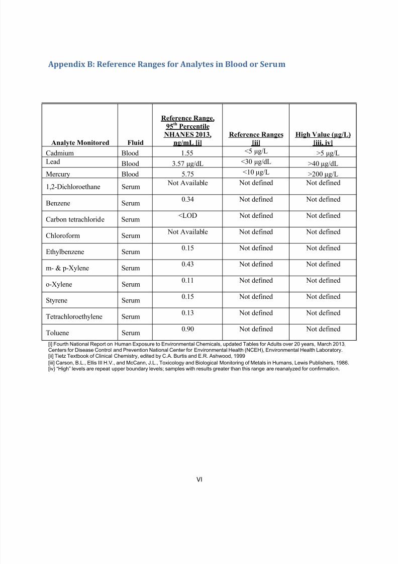
Appendix B: Reference Ranges for Analytes in Blood or Serum (Provided by DHSS) .............................. VI

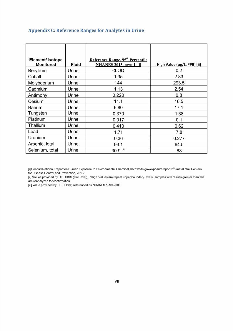
Appendix C: Reference Ranges for Analytes in Urine (Provided by DHSS) ............................................. VII

Appendix D: Data Quality Indicator Determination Methods ............................................................... VIII

Glossary ...................................................................................................................................................... XVI



v

List of FiguresFigure 1. Participant Sampling area (Red circle) with number of participants in each sector denoted

(including two replacement participants for 2012), Fixed Sites (Green), and NRG Energy power plant

(Yellow) during both Season 1 and 2 of the MIEBS Study. Note the Seaford monitor is not shown. .......... 6

Figure 2. Distributions of Seaford Site PM2.5, BrC, and BC concentrations during Season 1 (Red, NRG

Energy power plant not operating) & Season 2 (Blue, power plant operating) along with geometric

means (asterisks). Values below the MDL were assigned a value of the MDL divided by square root of 2.

.................................................................................................................................................................... 11

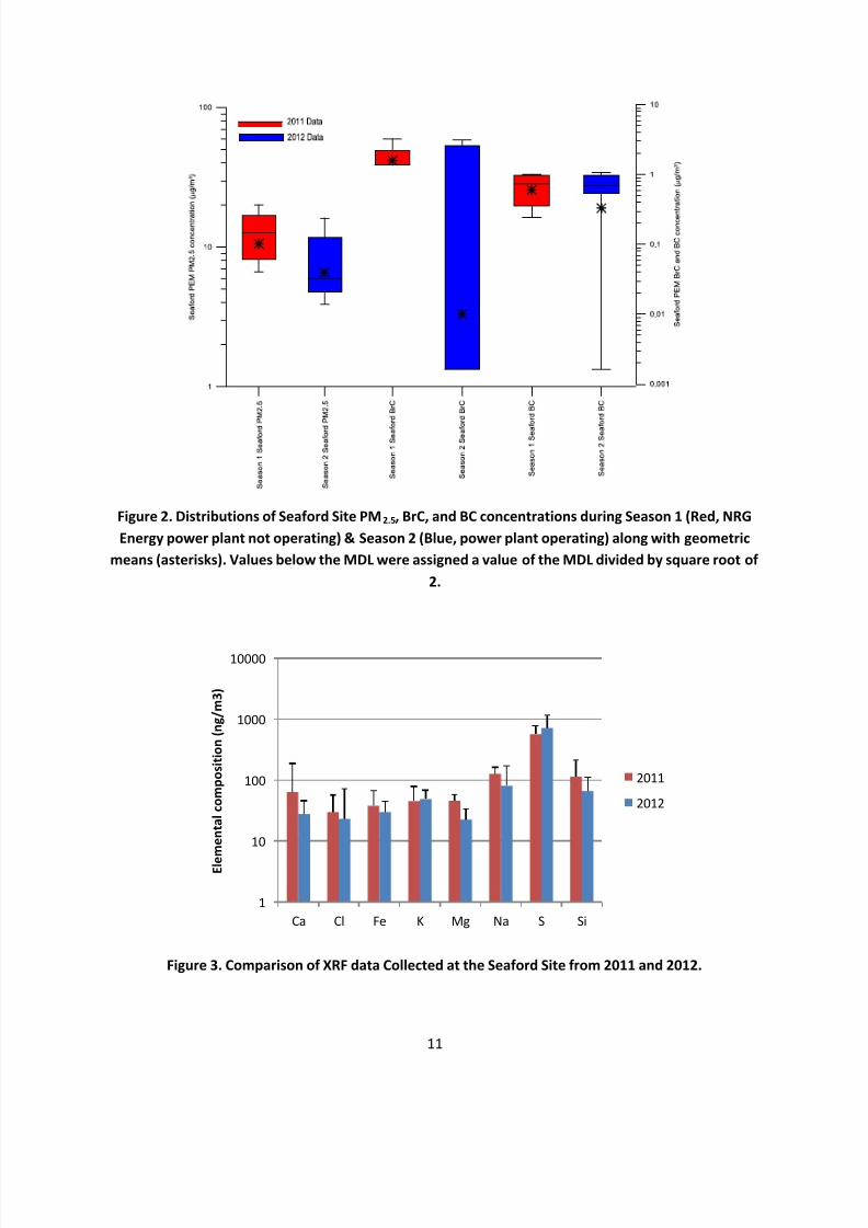
Figure 3. Comparison of XRF data Collected at the Seaford Site from 2011 and 2012. ............................. 11

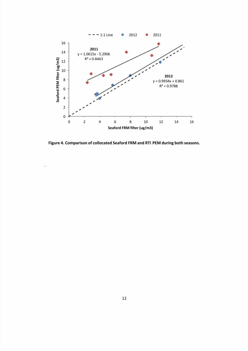
Figure 4. Comparison of collocated Seaford FRM and RTI PEM during both seasons. ............................... 12

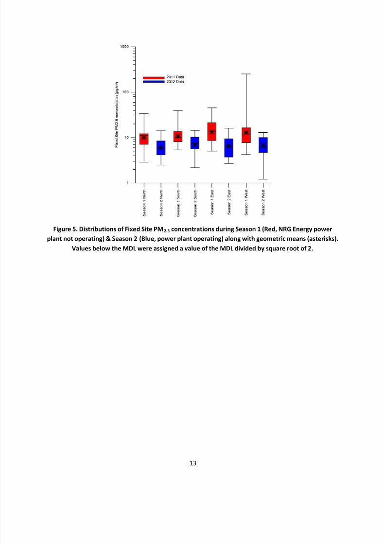
Figure 5. Distributions of Fixed Site PM2.5 concentrations during Season 1 (Red, NRG Energy power plant

not operating) & Season 2 (Blue, power plant operating) along with geometric means (asterisks). Values

below the MDL were assigned a value of the MDL divided by square root of 2. ....................................... 13

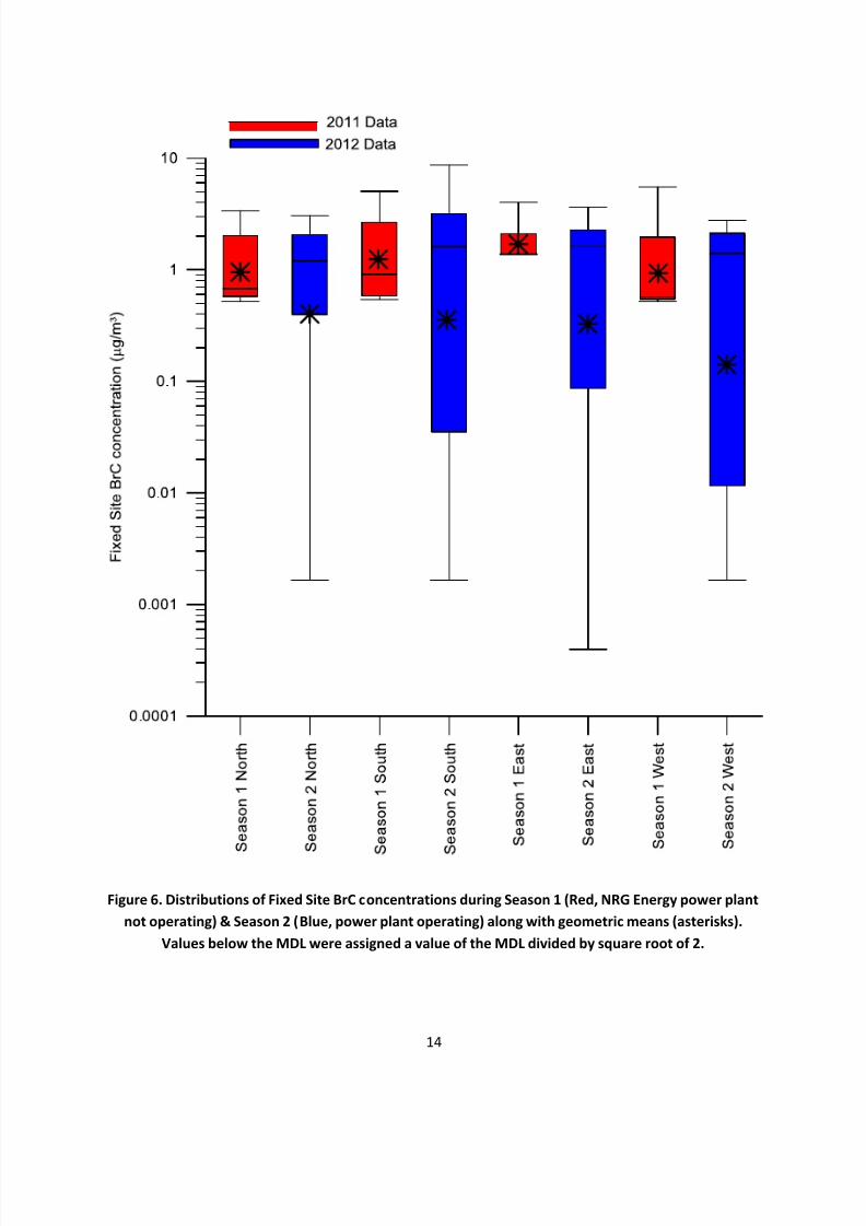
Figure 6. Distributions of Fixed Site BrC concentrations during Season 1 (Red, NRG Energy power plant



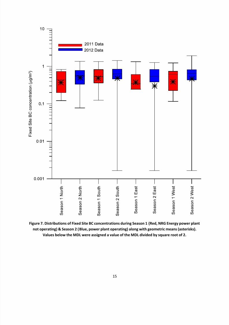
Figure 7. Distributions of Fixed Site BC concentrations during Season 1 (Red, NRG Energy power plant



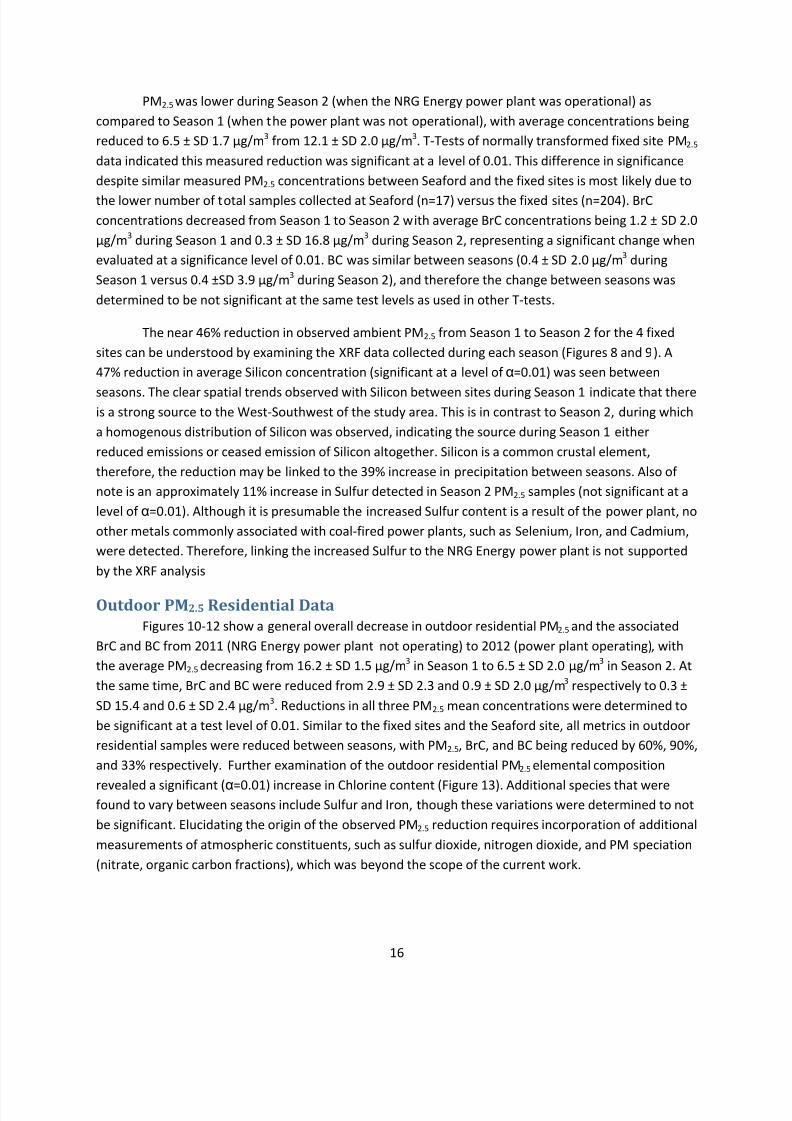
Figure 8. XRF Results from 2011 Fixed Site ambient samplers, Trace elements above MDL not shown. .. 17

Figure 9. XRF Results from 2012 Fixed Site ambient samplers, Trace elements above MDL not shown. .. 17

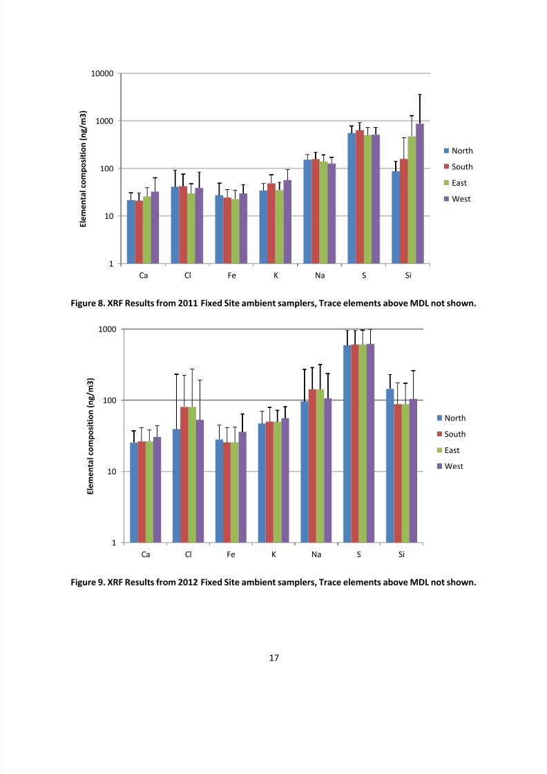
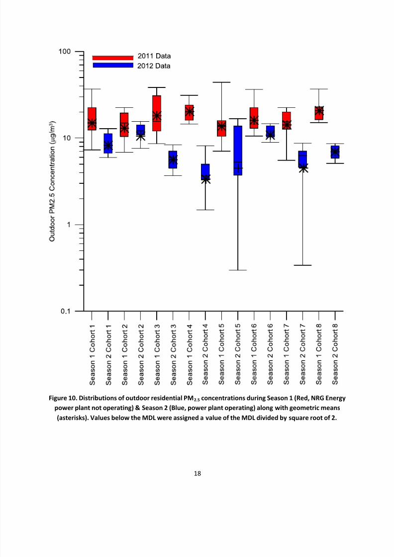
Figure 10. Distributions of outdoor residential PM2.5 concentrations during Season 1 (Red, NRG Energy

power plant not operating) & Season 2 (Blue, power plant operating) along with geometric means

(asterisks). Values below the MDL were assigned a value of the MDL divided by square root of 2. ......... 18

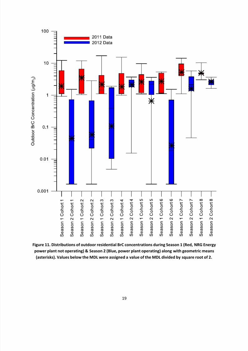
Figure 11. Distributions of outdoor residential BrC concentrations during Season 1 (Red, NRG Energy



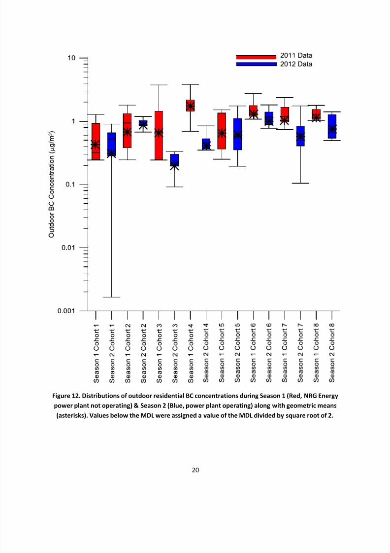
Figure 12. Distributions of outdoor residential BC concentrations during Season 1 (Red, NRG Energy



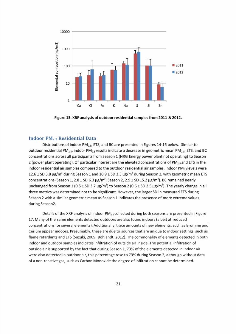
Figure 13. XRF analysis of outdoor residential samples from 2011 & 2012. .............................................. 21

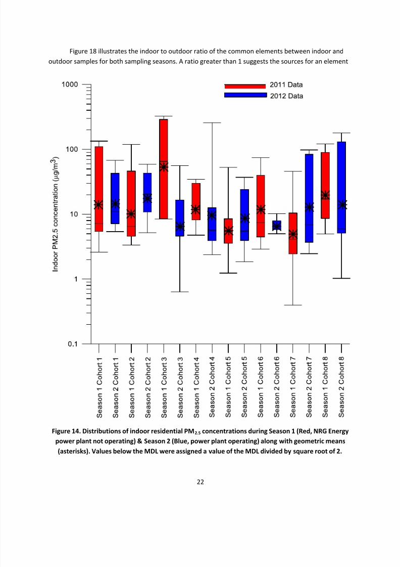
Figure 14. Distributions of indoor residential PM2.5 concentrations during Season 1 (Red, NRG Energy


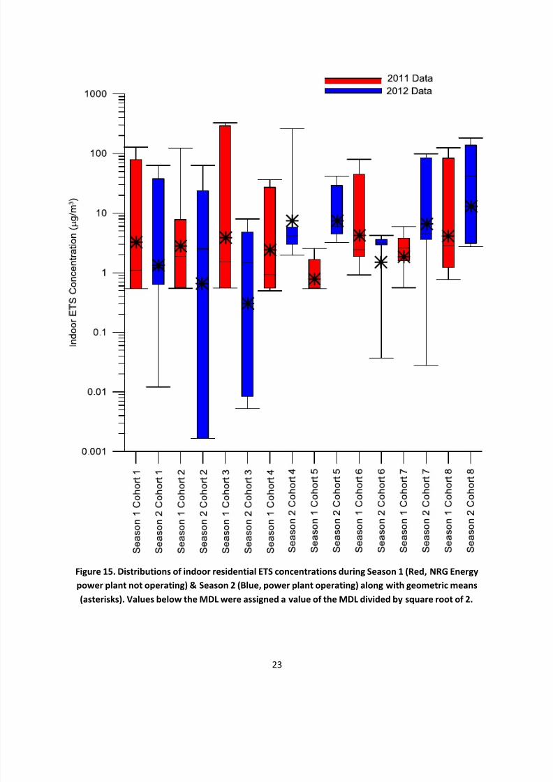
(asterisks). Values below the MDL were assigned a value of the MDL divided by square root of 2. ......... 22Figure 15. Distributions of indoor residential ETS concentrations during Season 1 (Red, NRG Energy







vii

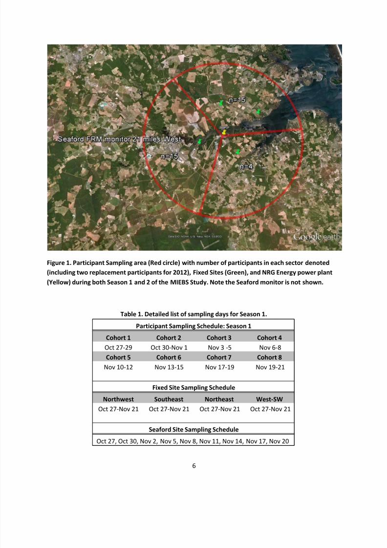
List of TablesTable 1. Detailed list of sampling days for Season 1. .................................................................................... 6

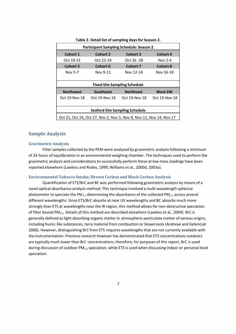
Table 2. Detail list of sampling days for Season 2. ........................................................................................ 7

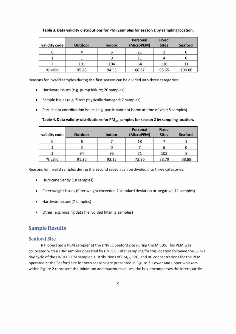
Table 3. Data validity distributions for PM2.5 samples for season 1 by sampling location............................ 9

Table 4. Data validity distributions for PM2.5 samples for season 2 by sampling location. .......................... 9

Table 5. Average temperatures and relative humidities for Season 1 & Season 2 participants. ............... 32

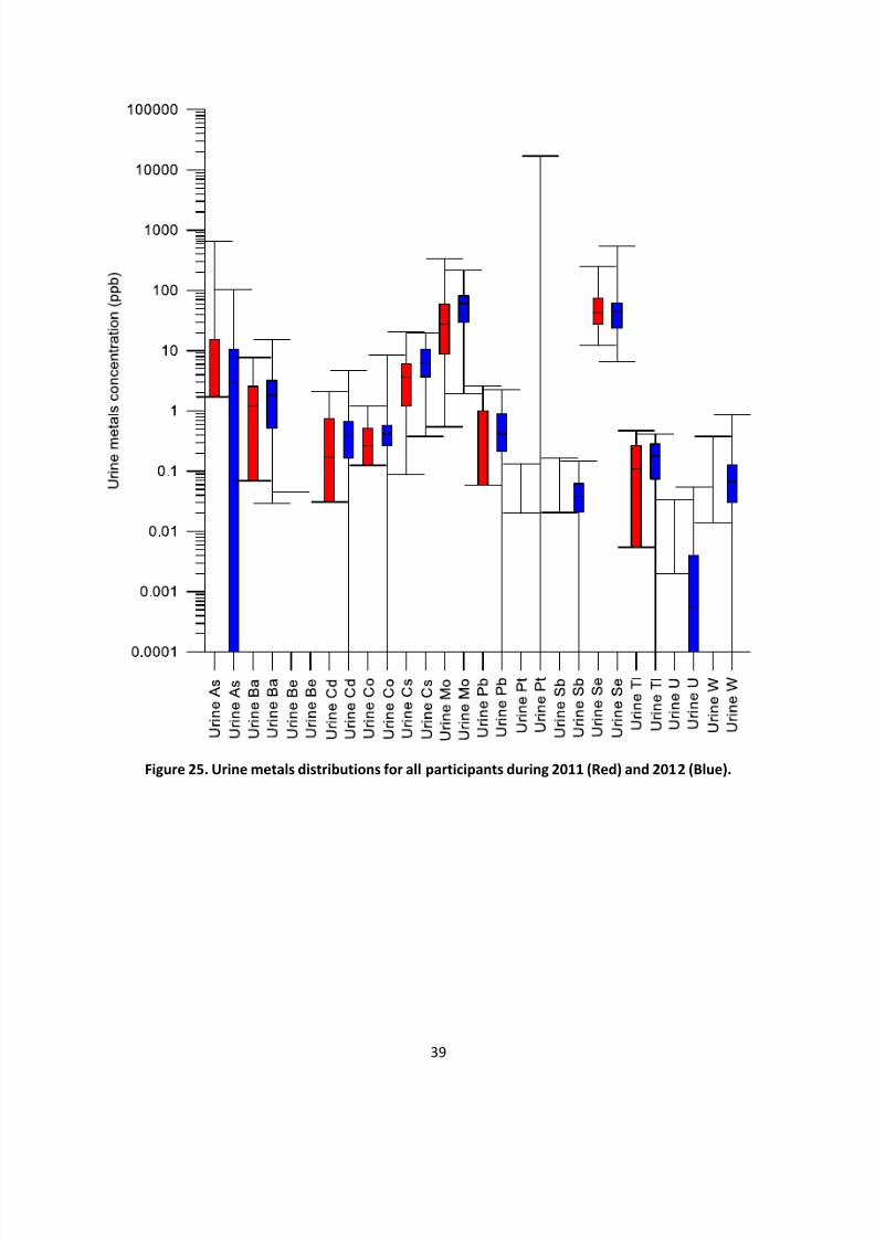
Table 6. 2011 Concentrations of metals in urine (ppb).[i] ........................................................................... 33

Table 7. 2012 Concentrations of metals in urine (ppb). [i] .......................................................................... 34

Table 8. 2011 and 2012 blood metals concentrations (ppb). ..................................................................... 35

Table 9. Participants for whom any of the analytes in blood or urine exceeded high reference value (*

indicates a measurement above the reference value). .............................................................................. 37

Table 10. Pearson correlations of PM mass with biospecimen elements by year. .................................... 40

Table 11. Pearson correlations of ETS mass with biospecimen elements by year. .................................... 41

Table 12. Pearson correlations of BC mass with biospecimen elements by year. ..................................... 43

Table 13.Pearson correlations of elements on personal filters by XRF with biospecimen elements by

year. ............................................................................................................................................................ 46

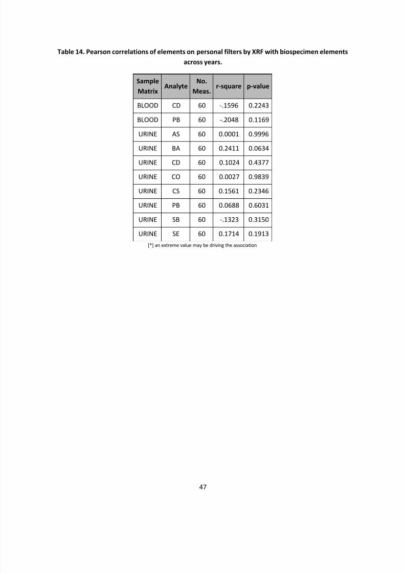
Table 14. Pearson correlations of elements on personal filters by XRF with biospecimen elements across

years. ........................................................................................................................................................... 47

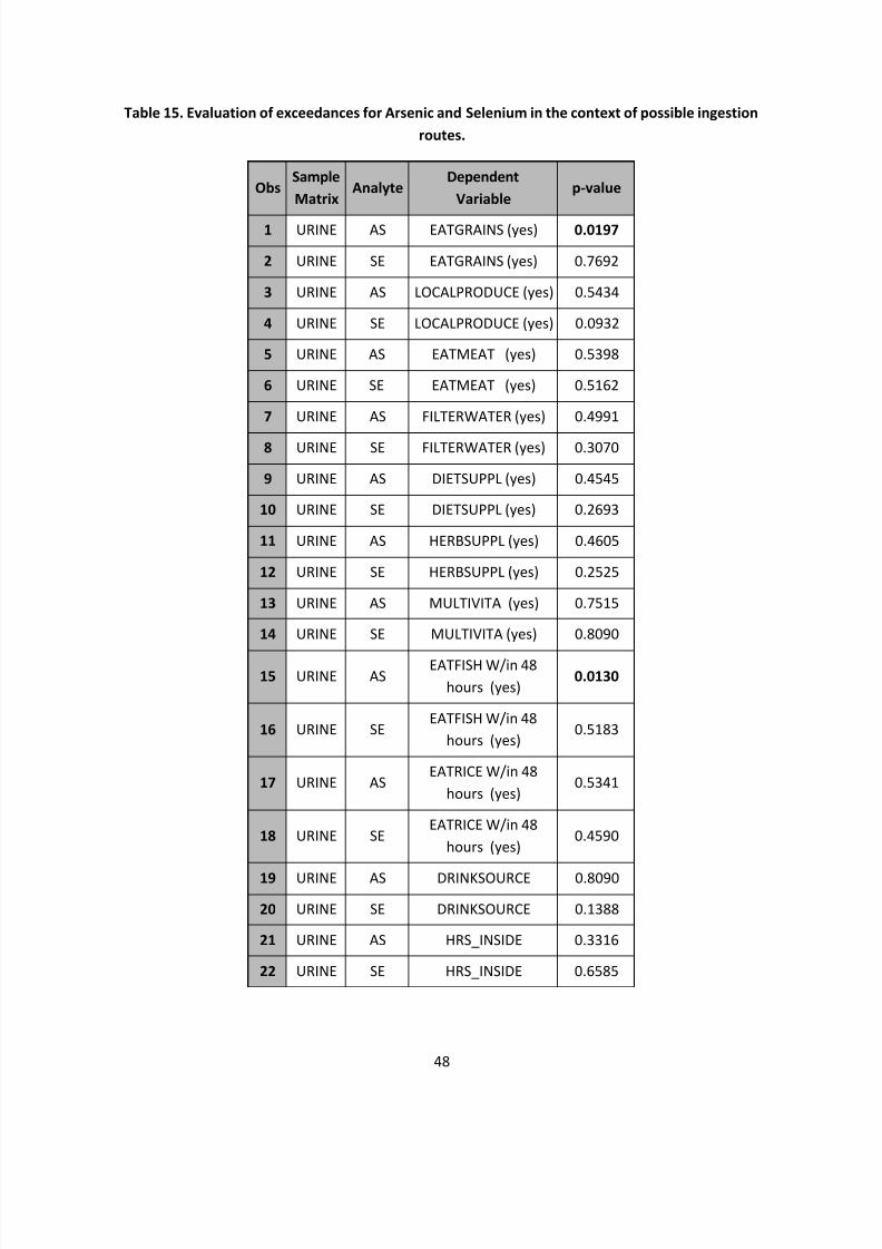
Table 15. Evaluation of exceedances for Arsenic and Selenium in the context of possible ingestion

routes. ......................................................................................................................................................... 48

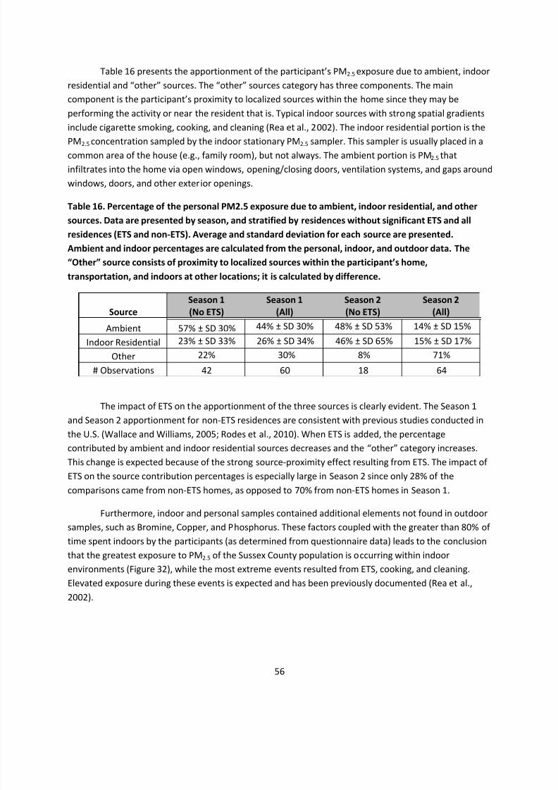
Table 16. Percentage of the personal PM2.5 exposure due to ambient, indoor residential, and other

sources. Data are presented by season, and stratified by residences without significant ETS and all

residences (ETS and non-ETS). Average and standard deviation for each source are presented. Ambient

and indoor percentages are calculated from the personal, indoor, and outdoor data. The “Other” source

consists of proximity to localized sources within the participant’s home, transportation, and indoors at

other locations; it is calculated by difference. ............................................................................................ 56

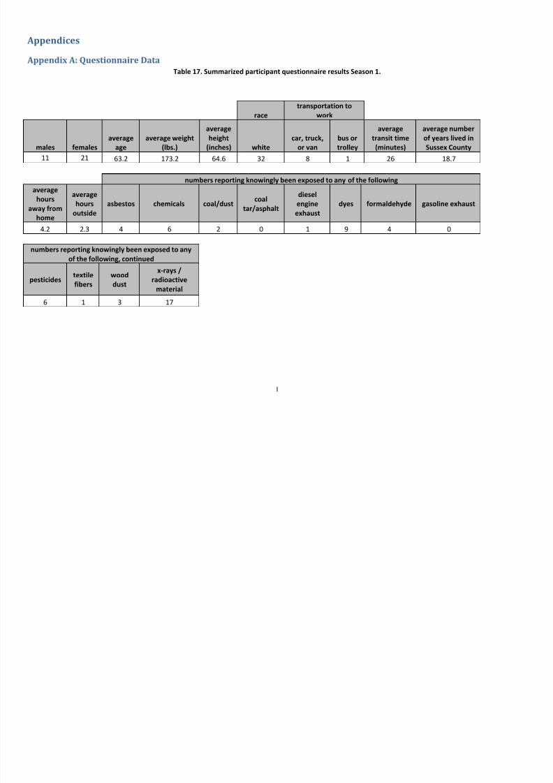
Table 17. Summarized participant questionnaire results Season 1. .............................................................. I

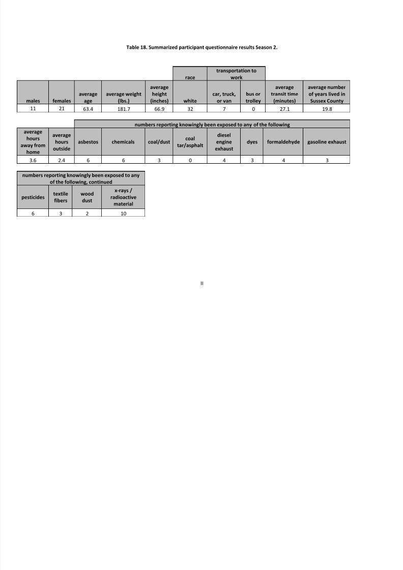
Table 18. Summarized participant questionnaire results Season 2. ............................................................. II

Table 19. Summarized residential questionnaire results Season 1. ............................................................ III

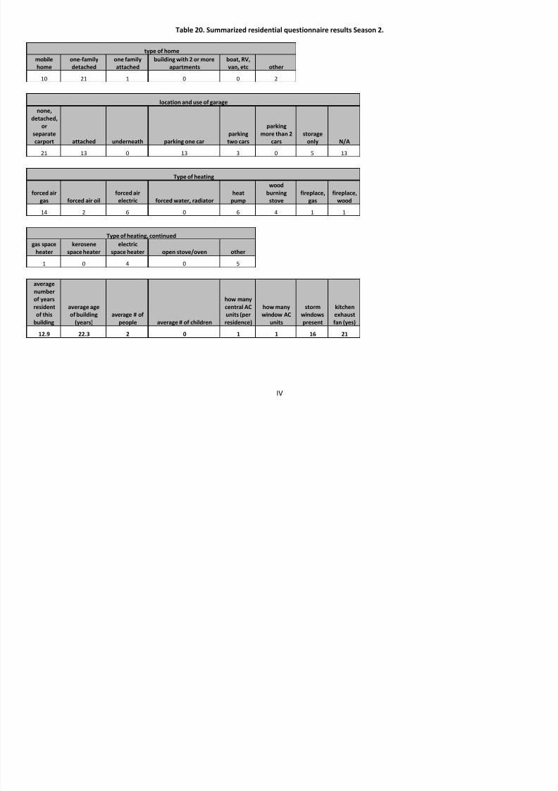
Table 20. Summarized residential questionnaire results Season 2. ............................................................ IV

Table 21. Summarized additional questionnaire data taken during season 2. ............................................ V

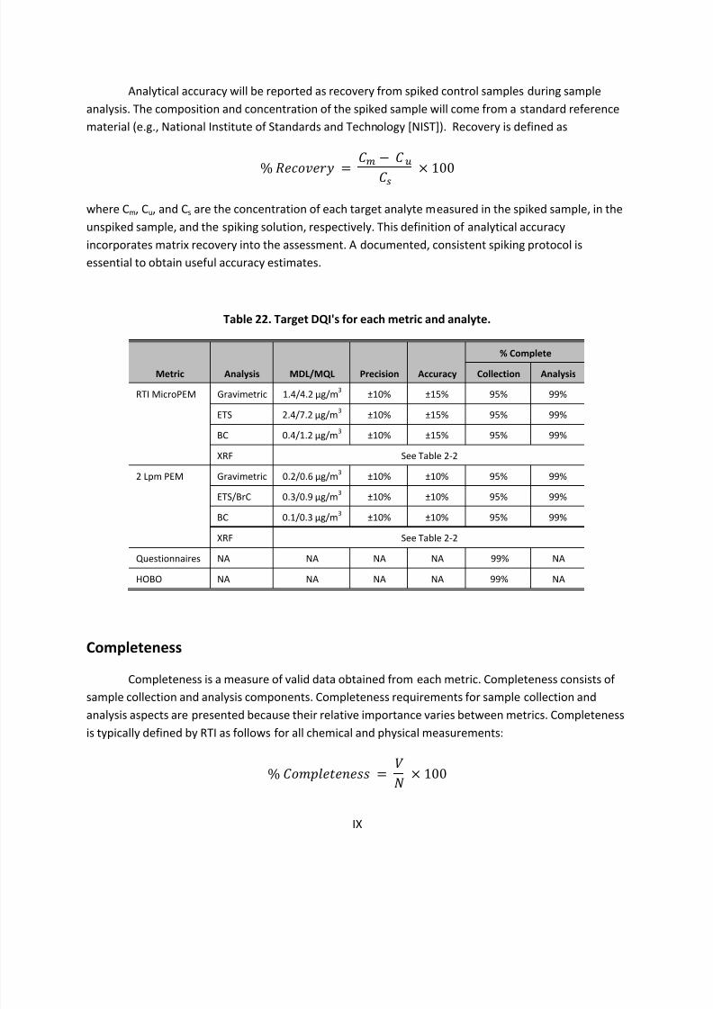
Table 22. Target DQI's for each metric and analyte. ................................................................................... IX

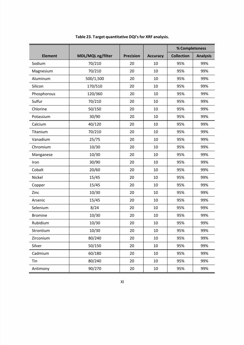
Table 23. Target quantitative DQI's for XRF analysis. .................................................................................. XI

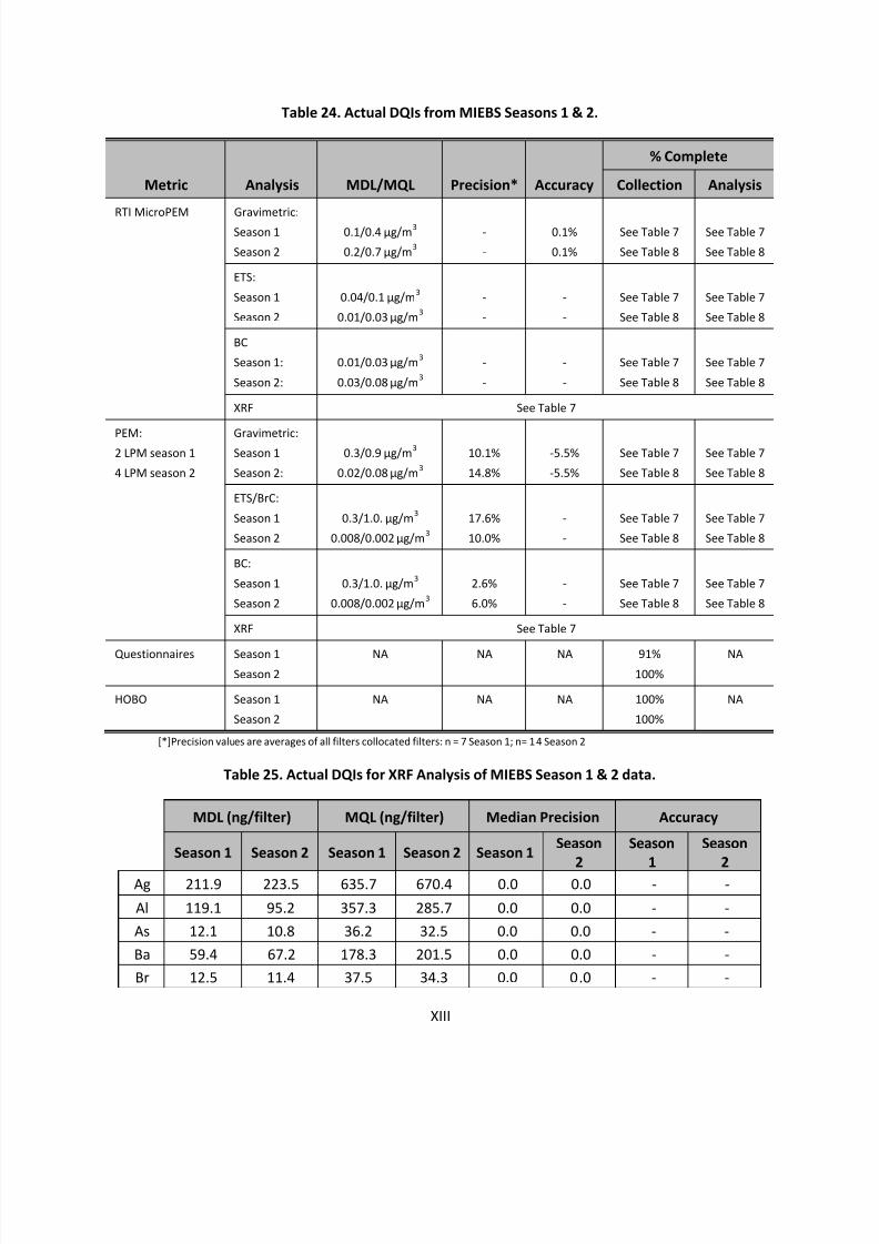
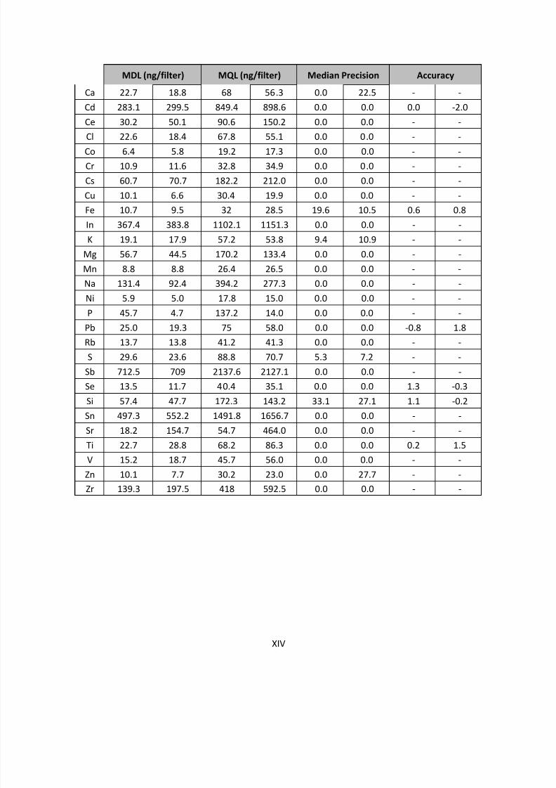
Table 24. Actual DQIs from MIEBS Seasons 1 & 2. .................................................................................... XIIITable 25. Actual DQIs for XRF Analysis of MIEBS Season 1 & 2 data. ........................................................ XIII



viii

ForwardThe Millsboro Inhalation Exposure and Biomonitoring Study (MIEBS) was performed to assess

the role of the NRG Energy power plant in Millsboro, Delaware in increasing the exposure of Sussex

County residents to particulate matter, metals, and selected organic contaminants. The study involved

the collection of outdoor air quality data, indoor air quality data, personal air quality data, biospecimen

data, and questionnaire data in the Fall of 2011 and the Fall of 2012. This report presents the objectives,

methods, results, and conclusions of the study.

This study has been a partnership between the Delaware Department of Natural Resources and

Environmental Control (DNREC) and the Delaware Department of Health and Social Services (DHSS),

with technical assistance from RTI International who was contracted to perform the environmental

sampling and analysis.



ix

AcknowledgmentsForemost, this study would not be possible without the participation and support of the Sussex

County residents. Thirty-five Sussex County residents participated in the study, while numerous others

expressed a willingness to participate.

This project was underwritten by the Delaware Department of Natural Resources and

Environmental Control and the Delaware Cancer Consortium, in collaboration with the Delaware Health

Fund.

Several RTI International (RTI) staff contributed significantly to this project. Dr. Jonathan

Thornburg and Dr. James Raymer were co-Principal Investigators. Dr. Quentin Malloy managed the daily

technical details of sample collection and analysis. Michael Philips recruited the study participants.

Cortina Johnson and Jocelin Deese-Spruill spent six weeks in Delaware in 2011 and 2012 working with

the participants to collect the particulate matter samples. Meaghan McGrath and Andrea McWilliams

analyzed the collected environmental samples. Larry Michael performed the statistical analysis of thedata. Lastly, Wayne Dawson is a Sussex County resident hired by RTI as a temporary contractor to assist

with sample collection.

RTI conducted this project in conjunction with the Delaware Department of Natural Resources

and Environmental Control (DNREC) and Delaware Health and Social Services Division of Public Health

(DPH). Elizabeth Frey (DNREC), Lisa Henry (DPH), and Richard Perkins (DPH) provided oversight of the

project. Mohammed Majeed (DNREC) performed air dispersion modeling to aid siting of the fixed site air

monitors and identify areas for participant recruitment. Susan Mitchell, R.N. (DPH) collected the

biological specimens from the participants. The Delaware Public Health Laboratory, under the direction

of Tara Lydick, analyzed the biological specimens. Richard Greene (DNREC) provided extensive

comments that improved the quality of this report.



x

List of Acronymsµg: Microgram

BC: Black Carbon

BrC: Brown Carbon

Cm: Measured concentration of a spiked sample

Cs: Measured concentration of a spiked solution

Csample: Measured concentration of a sample

Cstd: Measured concentration of a certified standard

Cu: Measured concentration of an unspiked sample

DHSS: Delaware Department of Health and Social Services

DNREC: Delaware Department of Natural Resources and Environmental Control

DPHL: Delaware Public Health Laboratory

DQI: Data Quality Indicator

ETS: Environmental Tobacco Smoke

FRM: Federal Reference Method

ICP-DRC/MS: Inductively Coupled Plasma-Dynamic Reaction Cell/Mass Spectrometry

ICP-MS: Inductively Coupled Plasma-Mass Spectrometry

LPM: Liter Per Minute

MDL: Minimum Detection Limit

MIEBS: Millsboro Inhalation Exposure and Biomonitoring Study

MQL: Minimum Quantification Limit

P/I: Personal-to-Indoor ratio

PEM: Personal Exposure Monitor

PM: Particulate Matter

PM2.5: Particulate Matter with an aerodynamic diameter equal to or less than 2.5 micrometers

RSD: Relative Standard Deviation

RTI: Research Triangle Institute

SD: Standard Deviation

SPME-GC: Solid-Phase Micro Extraction-Gas Chromatography

TAD: Time Activity Diary

VOC: Volatile Organic Compound

XRF: X-Ray Fluorescence



1

Introduction

Background

Evidence is increasing that long-term human exposure to particulate matter (PM) has negative

impacts on human health, including adverse respiratory and cardiovascular effects (Dockery 2001; Ito et

al. 2011). It has also been demonstrated that acute exposures to elevated PM can lead to a myriad of

health end points, including non-accidental mortality, total mortality, respiratory deaths, and morbidity

(Goldberg et al. 2001; Laden et al. 2000; Hoek et al. 2001; Zanobetti, Schwartz, and Dockery 2000).

However, there exists a need for more information about the amount and composition of this PM as it

relates to health end points of the exposed population. Those who live close to sources of PM2.5 (PM

with an aerodynamic diameter equal to or less than 2.5 micrometers) are especially vulnerable to the

negative impacts; therefore, federal and state agencies have made it a priority to gather more

information concerning the health outcomes of long-term exposure to these particles.

Research has shown the spatial gradients in PM2.5 to be smaller than PM10 (PM with an

aerodynamic diameter equal to or less than 10 micrometers) with concentrations being higher in urban

areas and close to point sources, but temporal trends are stronger with PM2.5 (Environment Canada-

Health Canada 2000; Thornburg et al. 2009; Rodes et al. 2010). It has also been noted that strong diurnal

trends exist with the chemical composition of PM2.5 (Cheung et al. 2011). Many factors influence these

gradients, including temperature, wind direction, and human activity patterns. Because of the regional

nature of PM2.5, the adverse health effects associated with it are more widespread and can be harder to

link to specific sources. This is especially compounded by the paucity of personal exposure data.

Study Purpose and Goals

This study centers around the DESIGN I plan presented to the Department of Natural Resources

and Environmental Control (DNREC) by RTI International in June 2008 (DNREC-OTS, 2008). The DESIGN I

plan described a multi-media exposure study in Sussex County that would serve as a pilot effort as a

prelude to a statewide study. The scope of the DESIGN I plan was reduced in accordance with the

available budget resources. The final study design yielded the Millsboro Inhalation Exposure and

Biomonitoring Study (MIEBS). Although MIEBS was developed to explore inhalation exposure pathways,

it is possible alternative exposure routes, such as seafood consumption, may be of interest though

outside the scope of MIEBS (Greene and Crecelius, 2006). MIEBS addressed four objectives over the

course of an 18-month study. MIEBS had the following objectives:

1) Evaluate the impacts of the NRG Energy power plant operating capacity on PM2.5 exposure levels

of the Sussex County population.

2) Ascertain the relative contributions of upwind sources in Virginia, Maryland, Pennsylvania, New

York, and the New England area on the PM2.5 exposure of the Sussex County population.

3) Establish the contribution of point, local, and personal sources to the Sussex County

population’s exposure to PM2.5.

4) Collect biological samples for dose measurements of the Sussex County population.



2

Objectives one, two, and three focused on the NRG Energy power plant, other ambient sources, and

residential sources and their impact on the inhalation exposures of the surrounding Sussex County

population. Objective four attempted to link the participants PM2.5 exposures to their dose of specific

chemical species.

Data for Objective 1—

Evaluation of NRG Energy Power Plant Operating CapacityTo evaluate the effect of the NRG Energy power plant operating capacity on PM2.5 exposures of

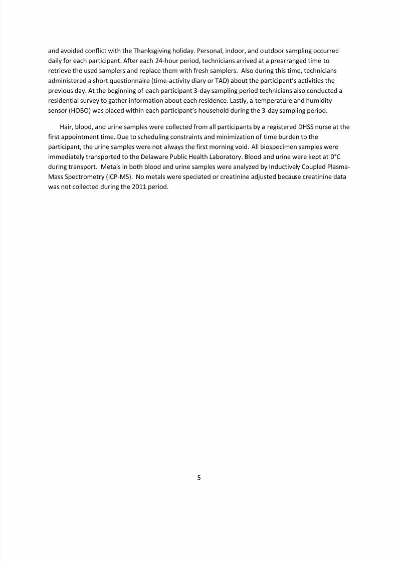
the Sussex County population, air samples were collected in a variety of locations over the course of two

periods (non-operating and operating). The locations included fixed site monitors located upwind and

downwind of the power plant. In addition to the fixed sites, samples were taken outside and inside

participants’ houses along with personal air samples. It should be noted that NRG Energy power

electricity generation load fluctuated daily during the second season.

Measurements for this objective included not only PM2.5 mass, but also PM2.5 composition,

which included environmental tobacco smoke (ETS), brown carbon (BrC), black carbon (BC), and metals.

Metals were identified for analysis based on previous studies by DNREC (DNREC, 2006) along with thecurrent U.S. Environmental Protection Agency (EPA) criteria document (U.S. EPA 2004).

Data for Objective 2—Contribution of Out-of-State Sources to Sussex County PM2.5 Exposures

In addition to evaluating the effect of the NRG Energy power plant operating capacity, RTI

determined the relative contribution of sources in upwind states such as Pennsylvania, Maryland, and

Virginia to Sussex County PM2.5. For this objective, meteorological data and optimal spatial distribution

of monitors was key. Data from the same samples were used to address Objectives 1 and 2 through

proper spatial planning of sampler deployment.

Data for Objective 3—Contribution of Other Sources to PM2.5 Exposure

Data collection for Objective 3 used the same sampling platforms as used in Objective 1. This

information was used to locate potential sources of PM2.5 other than the NRG Energy power plant,

which could significantly contribute to the exposure of the Sussex County population. The

questionnaires and permitting database mining were used in conjunction with the personal sampling to

gather detailed data concerning personal exposures.

Data for Objective 4—Collect Biological Specimens

Blood, hair, and urine samples were collected from each participant once during each sampling

campaign. These biospecimens were used to investigate changes in personal PM2.5 measures (mass, ETS)

with changes in human exposure. Of particular interest were changes in PM2.5 that might be associated

with the NRG Energy power plant. Blood and urine samples were analyzed by DHSS. Blood samples were

analyzed for VOCs and metals and urine samples were analyzed for metals. Blood, urine, and hair were

archived for potential future analysis of other environmental pollutants. Blood and urine samples were

archived at -80C.



3

Hypotheses

The hypotheses for each objective are outlined below. The details describing how each

hypothesis was tested are provided in more detail in the following section.

Objective 1

Hypothesis 1: Contributions of the NRG Energy power plant to ambient PM2.5 concentrations in Sussex

County will increase with increasing usage of the electricity generating capacity of the power plant.

Indoor residential and personal PM2.5 concentrations will not be affected.

Objective 2

Hypothesis 2: Upwind source contributions to ambient Sussex County PM2.5 levels will be detectable,

and their relative contribution to the PM2.5 concentration will decrease as the load on the NRG Energy

power plant increases. However, exact sources will be difficult to determine unless a unique emissions

profile exists.

Hypothesis 3: The relative contribution of upwind sources from bordering states to the ambient PM2.5

concentration will decrease as usage of the energy generating capacity from the NRG Energy power

plant increases.

Objective 3

Hypothesis 4: Relative contributions of other point PM2.5 sources to ambient concentrations will

decrease after the NRG Energy power plant increases its electricity generation.

Hypothesis 5: Personal sources will contribute more to PM2.5 exposure relative to during the low

electricity generation period than during the high generation sampling period.

Objective 4

Hypothesis 6: Markers for PM2.5 exposure from NRG Energy power plant emissions in biological

specimens will increase as the load demand on the power plant increases.

Report Framework

The structure of this report presents the study methodology, data quality summary, PM2.5

concentration and biospecimen data presentation, evaluation of the hypotheses, and the study

conclusions/recommendations. The study methodology summarizes the study area, participants, and

sample collection methods. The data quality summary provides an overview of data capture for each

metric, including reasons for invalid samples. Subsequent sections present PM2.5 concentrations from

each sampling season along with corresponding environmental tobacco smoke (ETS) and black carbon

(BC) measurements. Particulate metals analysis performed by X-ray fluorescence (XRF) is also presented

during discussion of results from each sample type. Following the data presentation, discussion of the



4

study objectives and hypotheses in the context of the previously presented data is performed followed

by conclusions and recommendations by RTI.

Study Methodology

RTI conducted two sampling periods for the MIEBS in October through November of 2011 and

October through November of 2012. Data acquired during the first sampling campaign (hereinafter

referred to as Season 1) captured PM concentrations while the NRG Energy power plant was shut-down

for the installation of pollution control technologies. The second campaign (hereinafter referred to

Season 2) took place after the power plant had resumed operation. Sample collection consisted of

personal exposure, residential indoor, residential outdoor, and ambient fixed site monitoring. Figure 1

presents the area of Sussex County sampled, and the three sectors where recruited participants reside.

Four fixed site ambient monitors near the power plant are also shown; the DNREC ambient monitoring

site, not shown, is located in Seaford, Delaware.

Multiple types of personal exposure monitors collected PM2.5 filter samples. RTI used the

MicroPEM to collect PM2.5 personal exposure samples. Participants wore the MicroPEM unit during

their normal, daily activities. Participants did not wear the unit while bathing or sleeping. The MicroPEM

operated at 0.5 LPM and collected PM2.5 on a 25 mm Teflo® filter (Gelman Sciences, Ann Arbor,

Michigan, 3 µm porosity) during both seasons. Participants during the second season used MicroPEM

units that also contained nephelometers which permitted real-time PM2.5 mass concentration to be

collected. RTI deployed Personal Exposure Monitors (PEMS, MSP Corporation, Minneapolis, MN) as

stationary residential indoor, residential outdoor, and ambient PM2.5 samplers. A PEM unit is a single

channel PM2.5 inlet operating at either 2 or 4 liters per minute (LPM) with a 37 mm Teflo filter and 2 µm

porosity.

RTI recruited and enrolled 32 participants for each season. Participant retention was high, with

29 recruits (91%) participating in both sampling seasons. Three replacement participants were recruited

in 2012 from the same sector (Figure 1) as the participants that withdrew. Participants were grouped

into eight cohorts of 4 participants each. There was no constraints put on participant involvement for

smokers, nor was questionnaire data collected that related to their smoking habits. Eight participants

per week were scheduled to complete the campaign within the 4-week window available. The exception

to this was during the second sampling season when Hurricane Sandy forced a suspension in all

sampling activities during the course of four days (October 29-November 1).

The five fixed sites operated continuously with filters being replaced every 24 hours, except at

the Seaford site, which operated on a 1-in-3 day schedule corresponding to the DNREC PM2.5 FRM

monitor. The four 24-hour fixed site monitors were located within a 2.5 mile radius of the power plant,

whereas the Seaford site was located 21-miles west of the power plant, therefore data obtained from

the Seaford site is presented separately in order to uncover potential regional transport of power plant

associated PM2.5. Tables 1 and 2 provide a detailed overview of the sampling schedule and frequency of

visits during the each campaign. The appointment schedule minimized time burdens on the participants



5

and avoided conflict with the Thanksgiving holiday. Personal, indoor, and outdoor sampling occurred

daily for each participant. After each 24-hour period, technicians arrived at a prearranged time to

retrieve the used samplers and replace them with fresh samplers. Also during this time, technicians

administered a short questionnaire (time-activity diary or TAD) about the participant’s activities the

previous day. At the beginning of each participant 3-day sampling period technicians also conducted a

residential survey to gather information about each residence. Lastly, a temperature and humidity

sensor (HOBO) was placed within each participant’s household during the 3-day sampling period.

Hair, blood, and urine samples were collected from all participants by a registered DHSS nurse at the

first appointment time. Due to scheduling constraints and minimization of time burden to the

participant, the urine samples were not always the first morning void. All biospecimen samples were

immediately transported to the Delaware Public Health Laboratory. Blood and urine were kept at 0°C

during transport. Metals in both blood and urine samples were analyzed by Inductively Coupled Plasma-

Mass Spectrometry (ICP-MS). No metals were speciated or creatinine adjusted because creatinine data

was not collected during the 2011 period.



6

Figure 1. Participant Sampling area (Red circle) with number of participants in each sector denoted

(including two replacement participants for 2012), Fixed Sites (Green), and NRG Energy power plant

(Yellow) during both Season 1 and 2 of the MIEBS Study. Note the Seaford monitor is not shown.

Table 1. Detailed list of sampling days for Season 1.

Participant Sampling Schedule: Season 1

Cohort 1 Cohort 2 Cohort 3 Cohort 4

Oct 27-29 Oct 30-Nov 1 Nov 3 -5 Nov 6-8


Nov 10-12 Nov 13-15 Nov 17-19 Nov 19-21

Fixed Site Sampling Schedule

Northwest Southeast Northeast West-SW

Oct 27-Nov 21 Oct 27-Nov 21 Oct 27-Nov 21 Oct 27-Nov 21

Seaford Site Sampling Schedule

Oct 27, Oct 30, Nov 2, Nov 5, Nov 8, Nov 11, Nov 14, Nov 17, Nov 20



7

Table 2. Detail list of sampling days for Season 2.

Participant Sampling Schedule: Season 2


Oct 19-21 Oct 22-24 Oct 26 -28 Nov 2-4


Nov 5-7 Nov 9-11 Nov 12-14 Nov 16-18

Fixed Site Sampling Schedule

Northwest Southeast Northeast West-SW

Oct 19-Nov 18 Oct 19-Nov 18 Oct 19-Nov 18 Oct 19-Nov 18

Seaford Site Sampling Schedule

Oct 21, Oct 24, Oct 27, Nov 2, Nov 5, Nov 8, Nov 11, Nov 14, Nov 17

Sample Analysis

Gravimetric Analysis

Filter samples collected by the PEM were analyzed by gravimetric analysis following a minimum

of 24 hours of equilibration in an environmental weighing chamber. The techniques used to perform the

gravimetric analysis and considerations to successfully perform these at low mass loadings have been

reported elsewhere (Lawless and Rodes, 1999; Williams et al., 2000d, 2003a).

Environmental Tobacco Smoke/Brown Carbon and Black Carbon Analysis

Quantification of ETS/BrC and BC was performed following gravimetric analysis by means of a

novel optical absorbance analysis method. This technique involved a multi-wavelength spherical

photometer to speciate the PM2.5 determining the absorbance of the collected PM2.5 across several

different wavelengths. Since ETS/BrC absorbs at near UV wavelengths and BC absorbs much more

strongly than ETS at wavelengths near the IR region, this method allows for non-destructive speciation

of filter bound PM2.5. Details of this method are described elsewhere (Lawless et al., 2004). BrC is

generally defined as light absorbing organic matter in atmospheric particulate matter of various origins,

including humic like substances, tarry material from combustion or bioaerosols (Andreae and Gelencsér

2006). However, distinguishing BrC from ETS requires wavelengths that are not currently available with

the instrumentation. Previous research however has demonstrated that ETS concentrations outdoors

are typically much lower than BrC concentrations; therefore, for purposes of this report, BrC is used

during discussion of outdoor PM2.5 speciation, while ETS is used when discussing indoor or personal level

speciation.



8

X-Ray Fluorescence Analysis

Following gravimetric and optical analysis, the Teflon filters were analyzed for selected elements

by X-ray fluorescence (XRF). Details about the normal XRF operational procedures employed for these

types of samples have been reported by Dzubay et al. (1988) and Landis et al. (2001).

Urine AnalysisUrine samples were tested by Delaware Public Health Laboratory (DPHL) for trace metals (Ba,

Be, Cd, Co, Cs, Mo, Pb, Pt, Sb, Tl, U, W) by inductively coupled plasma mass spectrometry (ICP/MS) and

inductively coupled dynamic reaction cell-plasma mass spectrometry (ICP-DRC/MS) (As, Se). This

method utilizes small volumes of urine that are spiked with known internal standard solution in an

acidified dilute matrix. The method is based upon that utilized by the Centers for Disease Control and

Prevention. Plasma is used to ionize the sample and mass spectrometric scanning of resulting specific

isotopes to identify the metal species in question. A DRC is used for As and Se to reduce the possibility of

interferences from isobaric, doubly charged, and polyatomic species. This provides excellent accuracy,

specificity, dynamic range, precision, and multi-element capability. No metals were speciated or

creatinine adjusted.

Blood Analysis

DPHL analyzed blood metals (Cd, Hg, Pb) by ICP/MS. This method utilizes small volumes of blood

that are spiked with known internal standard solution in a basic diluent matrix. Similar to urine analysis,

blood samples are ionized and then a mass spectrometer scans the resulting specific isotopes to identify

the metals in question.

Blood Volatile Organic Compounds (VOCs) were analyzed by isotope dilution solid phase micro

extraction gas chromatography (SPME-GC/MS). This method utilizes small volumes of blood that are

spiked with known isotopically labeled internal standard solution. A microfiber is used to absorb the

volatile components released from the blood in the head space of the vial when heated. The

components are then desorbed into a heated inlet, separated via GC, ionized, then fragmented into

charged fragments which are collected and separated on the basis of their mass / charge ratio with the

mass spectrometer. This method is based on a method used by the Centers for Disease Control and

Prevention.

Data Quality ResultsTables 3 and 4 present data capture rate for 2011 and 2012 by sample type. Sample collection

during each sampling season was generally in excess of 90%.



9

Table 3. Data validity distributions for PM2.5 samples for season 1 by sampling location.

validity code Outdoor Indoor

Personal

(MicroPEM)

Fixed

Sites Seaford

0 4 6 21 1 0

1 1 0 11 4 02 101 104 64 110 11

% valid 95.28 94.55 66.67 95.65 100.00

Reasons for invalid samples during the first season can be divided into three categories:

Hardware issues (e.g. pump failure; 20 samples)

Sample issues (e.g. filters physically damaged; 7 samples)

Participant coordination issues (e.g. participant not home at time of visit; 5 samples)

Table 4. Data validity distributions for PM2.5 samples for season 2 by sampling location.

validity code Outdoor Indoor

Personal

(MicroPEM)

Fixed

Sites Seaford

0 6 7 18 7 1

1 3 0 7 6 0

2 94 95 71 103 8

% valid 91.26 93.13 73.96 88.79 88.88

Reasons for invalid samples during the second season can be divided into three categories:

Hurricane Sandy (18 samples)

Filter weight issues (filter weight exceeded 2 standard deviation or negative; 11 samples)

Hardware issues (7 samples)

Other (e.g. missing data file, voided filter; 3 samples)

Sample Results

Seaford Site

RTI operated a PEM sampler at the DNREC Seaford site during the MIEBS. This PEM was

collocated with a FRM sampler operated by DNREC. Filter sampling for this location followed the 1-in-3

day cycle of the DNREC FRM sampler. Distributions of PM2.5, BrC, and BC concentrations for the PEM

operated at the Seaford site for both seasons are presented in Figure 2. Lower and upper whiskers

within Figure 2 represent the minimum and maximum values, the box encompasses the interquartile



10

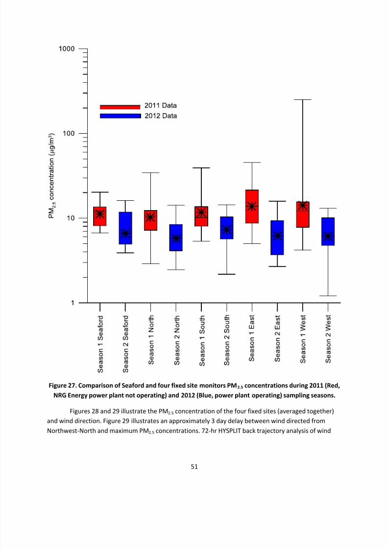
range (25th percent to 75th percent) of the data; the horizontal line in the box represents the median or

50th percentile value; and the star represents the arithmetic average of the data. All subsequent data

presented as box-and-whisker plots within this report all conform to this standard.

PM2.5 data for the Seaford monitoring site were lognormally distributed. Geometric mean PM2.5

concentrations during Season 2 (6.7 ± SD 1.6 µg/m3

) were reduced by 40% in comparison to Season 1concentrations (11.1 ± SD 1.5 µg/m3). BrC was also reduced from Season 1 to Season 2, with

concentrations dropping from 1.7 ± SD 1.4 µg/m3 during Season 1 to 0.01 ± SD 31.6 µg/m3 during Season

2. This trend in decreasing PM2.5 from Season 1 to Season 2 continued with BC decreasing between

Season 1 (0.6 ± SD 1.7 µg/m3) and Season 2 (0.34 ± SD 8.8 µg/m3). After transformation of the data to a

normal distribution, T-Test’s of the PM2.5, BrC, and BC indicate that the differences of means between

seasons were not significant at an alpha value of 0.01. Operating capacity of the NRG Energy power

plant was not available during the 2012 sampling period, therefore a correlation between PM2.5

reductions with power plant operation was not possible.

Evaluation of the XRF data (Figure 3) collected during the two sampling seasons reveals thatalthough there was a 26% increase in Sulfur content during this time, it was accompanied by reductions

in most other elements, including Calcium (56%), Chlorine (22%), Iron (21%), Magnesium (51%), Sodium

(37%), and Silicon (41%). T-Tests (α=0.01) of the normally transformed results between seasons

indicates that there are no significant differences with the exception of Magnesium, which had a P-value

of 0.0002. Because most of the elements that were reduced in mass between the two seasons originate

from crustal material, they are most prevalent in their oxide form, a fact which could account for the

overall mass reduction from Season 1 to Season 2.

Figure 4 illustrates the comparison between the Seaford FRM PM2.5 concentration and the RTI

collocated PEM sampler for both seasons (not blank corrected). The first season showed a reasonable

correlation (R-squared =0.85). However, the Seaford FRM samples were biased low, possibly due to the

increased face velocity of the FRM inducing additional volatilization of filter bound nitrate as has been

documented in comparison of PM2.5 filters with different filter face velocities (CARB, 1998). The FRM has

a face velocity five times greater than the 2 LPM PEM. In contrast to Season 1, comparison of RTI PEM

from Season 2 and Seaford FRM samples showed extremely good agreement, with a correlation

coefficient of 0.98. This increased correlation could be due to increased filter face velocity of RTI PEMs

during the switch to 4 LPM samplers which have a face velocity equal to 40% of the FRM.

Fixed Site Data

PEM samplers were attached to permanent structures at four locations (North, South, East, and

West) within approximately 2.5 miles of the NRG Energy power plant. These fixed site samplers

operated continuously for 24 hours, with filters from these samplers being collected each day

throughout the sampling phase. Fixed site samplers during Season 1 operated at 2 LPM, while Season 2

samplers were operated at 4 LPM. Figures 5-7 below detail the PM2.5, BrC, and BC concentration

distributions at these sites during Season 1 and Season 2.



11

Figure 2. Distributions of Seaford Site PM2.5, BrC, and BC concentrations during Season 1 (Red, NRG

Energy power plant not operating) & Season 2 (Blue, power plant operating) along with geometric

means (asterisks). Values below the MDL were assigned a value of the MDL divided by square root of

2.

Figure 3. Comparison of XRF data Collected at the Seaford Site from 2011 and 2012.

1

10

100

1000

10000

Ca Cl Fe K Mg Na S Si

E l e

m e n t a l c o m p o s i t i o n ( n g / m 3 )

2011

2012



12

Figure 4. Comparison of collocated Seaford FRM and RTI PEM during both seasons.

.

2012

y = 0.9934x + 0.861

R² = 0.9788

2011

y = 1.0615x - 5.2906

R² = 0.8463

0

2

4

6

8

10

12

14

16

0 2 4 6 8 10 12 14 16

S e a f o r d P E M

f i l t e r ( u g / m 3 )

Seaford FRM filter (ug/m3)

1:1 Line 2012 2011



13

Figure 5. Distributions of Fixed Site PM2.5 concentrations during Season 1 (Red, NRG Energy power

plant not operating) & Season 2 (Blue, power plant operating) along with geometric means (asterisks).

Values below the MDL were assigned a value of the MDL divided by square root of 2.



14

Figure 6. Distributions of Fixed Site BrC concentrations during Season 1 (Red, NRG Energy power plant

not operating) & Season 2 (Blue, power plant operating) along with geometric means (asterisks).




15

Figure 7. Distributions of Fixed Site BC concentrations during Season 1 (Red, NRG Energy power plant

not operating) & Season 2 (Blue, power plant operating) along with geometric means (asterisks).




16

PM2.5 was lower during Season 2 (when the NRG Energy power plant was operational) as

compared to Season 1 (when the power plant was not operational), with average concentrations being

reduced to 6.5 ± SD 1.7 µg/m3 from 12.1 ± SD 2.0 µg/m3. T-Tests of normally transformed fixed site PM2.5

data indicated this measured reduction was significant at a level of 0.01. This difference in significance

despite similar measured PM2.5 concentrations between Seaford and the fixed sites is most likely due to

the lower number of total samples collected at Seaford (n=17) versus the fixed sites (n=204). BrC

concentrations decreased from Season 1 to Season 2 with average BrC concentrations being 1.2 ± SD 2.0

µg/m3 during Season 1 and 0.3 ± SD 16.8 µg/m3 during Season 2, representing a significant change when

evaluated at a significance level of 0.01. BC was similar between seasons (0.4 ± SD 2.0 µg/m3 during

Season 1 versus 0.4 ±SD 3.9 µg/m3 during Season 2), and therefore the change between seasons was

determined to be not significant at the same test levels as used in other T-tests.

The near 46% reduction in observed ambient PM2.5 from Season 1 to Season 2 for the 4 fixed

sites can be understood by examining the XRF data collected during each season (Figures 8 and 9). A

47% reduction in average Silicon concentration (significant at a level of α=0.01) was seen between

seasons. The clear spatial trends observed with Silicon between sites during Season 1 indicate that thereis a strong source to the West-Southwest of the study area. This is in contrast to Season 2, during which

a homogenous distribution of Silicon was observed, indicating the source during Season 1 either

reduced emissions or ceased emission of Silicon altogether. Silicon is a common crustal element,

therefore, the reduction may be linked to the 39% increase in precipitation between seasons. Also of

note is an approximately 11% increase in Sulfur detected in Season 2 PM2.5 samples (not significant at a

level of α=0.01). Although it is presumable the increased Sulfur content is a result of the power plant, no

other metals commonly associated with coal-fired power plants, such as Selenium, Iron, and Cadmium,

were detected. Therefore, linking the increased Sulfur to the NRG Energy power plant is not supported

by the XRF analysis

Outdoor PM2.5 Residential Data

Figures 10-12 show a general overall decrease in outdoor residential PM2.5 and the associated

BrC and BC from 2011 (NRG Energy power plant not operating) to 2012 (power plant operating), with

the average PM2.5 decreasing from 16.2 ± SD 1.5 µg/m3 in Season 1 to 6.5 ± SD 2.0 µg/m3 in Season 2. At

the same time, BrC and BC were reduced from 2.9 ± SD 2.3 and 0.9 ± SD 2.0 µg/m3 respectively to 0.3 ±

SD 15.4 and 0.6 ± SD 2.4 µg/m3. Reductions in all three PM2.5 mean concentrations were determined to

be significant at a test level of 0.01. Similar to the fixed sites and the Seaford site, all metrics in outdoor

residential samples were reduced between seasons, with PM2.5, BrC, and BC being reduced by 60%, 90%,

and 33% respectively. Further examination of the outdoor residential PM2.5 elemental composition

revealed a significant (α=0.01) increase in Chlorine content (Figure 13). Additional species that werefound to vary between seasons include Sulfur and Iron, though these variations were determined to not

be significant. Elucidating the origin of the observed PM2.5 reduction requires incorporation of additional

measurements of atmospheric constituents, such as sulfur dioxide, nitrogen dioxide, and PM speciation

(nitrate, organic carbon fractions), which was beyond the scope of the current work.



17

Figure 8. XRF Results from 2011 Fixed Site ambient samplers, Trace elements above MDL not shown.

Figure 9. XRF Results from 2012 Fixed Site ambient samplers, Trace elements above MDL not shown.

1

10

100

1000

10000

Ca Cl Fe K Na S Si

E l e m e n t a l c o m p o s i t i o n ( n

g / m 3 )

North

South

East

West

1

10

100

1000

Ca Cl Fe K Na S Si

E l e m e n t a l c o m p o s i t i o n ( n g / m 3 )

North

South

East

West



18

Figure 10. Distributions of outdoor residential PM2.5 concentrations during Season 1 (Red, NRG Energy


(asterisks). Values below the MDL were assigned a value of the MDL divided by square root of 2.



19

Figure 11. Distributions of outdoor residential BrC concentrations during Season 1 (Red, NRG Energypower plant not operating) & Season 2 (Blue, power plant operating) along with geometric means




20

Figure 12. Distributions of outdoor residential BC concentrations during Season 1 (Red, NRG Energy





21

Figure 13. XRF analysis of outdoor residential samples from 2011 & 2012.

Indoor PM2.5 Residential Data

Distributions of indoor PM2.5, ETS, and BC are presented in Figures 14-16 below. Similar to

outdoor residential PM2.5, indoor PM2.5 results indicate a decrease in geometric mean PM2.5, ETS, and BC

concentrations across all participants from Season 1 (NRG Energy power plant not operating) to Season

2 (power plant operating). Of particular interest are the elevated concentrations of PM2.5 and ETS in the

indoor residential air samples compared to the outdoor residential air samples. Indoor PM2.5 levels were

12.6 ± SD 3.8 µg/m

3

during Season 1 and 10.9 ± SD 3.3 µg/m

3

during Season 2, with geometric mean ETSconcentrations (Season 1, 2.8 ± SD 6.3 µg/m3; Season 2, 2.9 ± SD 15.2 µg/m3). BC remained nearly

unchanged from Season 1 (0.5 ± SD 3.7 µg/m3) to Season 2 (0.6 ± SD 2.5 µg/m3). The yearly change in all

three metrics was determined not to be significant. However, the larger SD in measured ETS during

Season 2 with a similar geometric mean as Season 1 indicates the presence of more extreme values

during Season2.

Details of the XRF analysis of indoor PM2.5 collected during both seasons are presented in Figure

17. Many of the same elements detected outdoors are also found indoors (albeit at reduced

concentrations for several elements). Additionally, trace amounts of new elements, such as Bromine and

Cerium appear indoors. Presumably, these are due to sources that are unique to indoor settings, such as

flame retardants and ETS (Suzuki, 2009; Böhlandt, 2012). The commonality of elements detected in both

indoor and outdoor samples indicates infiltration of outside air inside. The potential infiltration of

outside air is supported by the fact that during Season 1, 73% of the elements detected in indoor air

were also detected in outdoor air, this percentage rose to 79% during Season 2, although without data

of a non-reactive gas, such as Carbon Monoxide the degree of infiltration cannot be determined.

1

10

100

1000

10000

Ca Cl Fe K Na S Si Zn

E l e m e n t a l c o m p o s t i o

n ( n g / m 3 )

2011

2012



22

Figure 18 illustrates the indoor to outdoor ratio of the common elements between indoor and

outdoor samples for both sampling seasons. A ratio greater than 1 suggests the sources for an element

Figure 14. Distributions of indoor residential PM2.5 concentrations during Season 1 (Red, NRG Energy





23

Figure 15. Distributions of indoor residential ETS concentrations during Season 1 (Red, NRG Energy





24

Figure 16. Distributions of indoor residential BC concentrations during Season 1 (Red, NRG Energy





25

Figure 17. Comparison of XRF analysis for indoor residential PM2.5 during 2011 & 2012.

Figure 18. Indoor residential-outdoor residential ratio of select elements.

1

10

100

1000

10000

Br Ca Ce Cl Cu Fe K Mg Na P S Si Zn

E l e m e n t a l c o m p o s i t i o

n ( n g / m 3 )

2011

2012



26

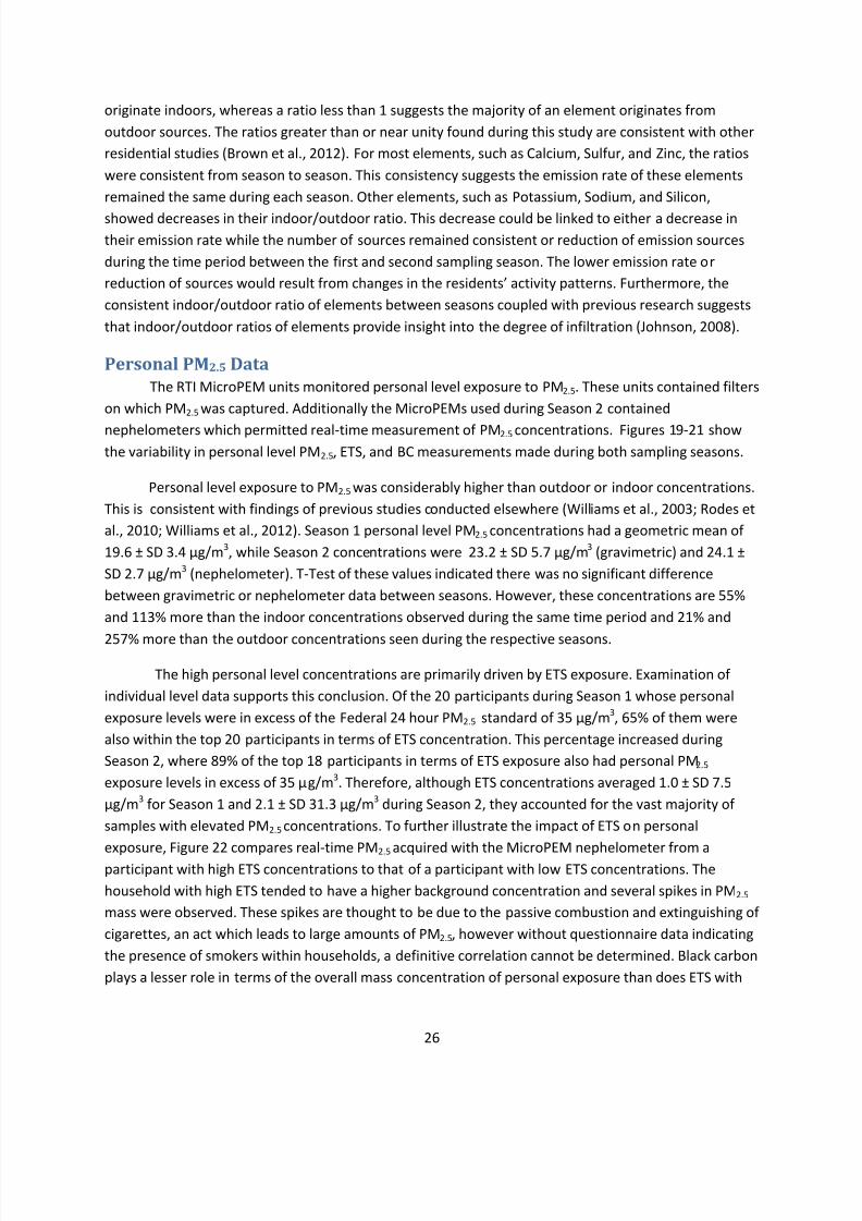
originate indoors, whereas a ratio less than 1 suggests the majority of an element originates from

outdoor sources. The ratios greater than or near unity found during this study are consistent with other

residential studies (Brown et al., 2012). For most elements, such as Calcium, Sulfur, and Zinc, the ratios

were consistent from season to season. This consistency suggests the emission rate of these elements

remained the same during each season. Other elements, such as Potassium, Sodium, and Silicon,

showed decreases in their indoor/outdoor ratio. This decrease could be linked to either a decrease in

their emission rate while the number of sources remained consistent or reduction of emission sources

during the time period between the first and second sampling season. The lower emission rate or

reduction of sources would result from changes in the residents’ activity patterns. Furthermore, the

consistent indoor/outdoor ratio of elements between seasons coupled with previous research suggests

that indoor/outdoor ratios of elements provide insight into the degree of infiltration (Johnson, 2008).

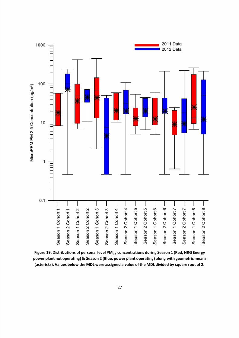
Personal PM2.5 Data

The RTI MicroPEM units monitored personal level exposure to PM2.5. These units contained filters

on which PM2.5 was captured. Additionally the MicroPEMs used during Season 2 contained

nephelometers which permitted real-time measurement of PM2.5 concentrations. Figures 19-21 showthe variability in personal level PM2.5, ETS, and BC measurements made during both sampling seasons.

Personal level exposure to PM2.5 was considerably higher than outdoor or indoor concentrations.

This is consistent with findings of previous studies conducted elsewhere (Williams et al., 2003; Rodes et

al., 2010; Williams et al., 2012). Season 1 personal level PM2.5 concentrations had a geometric mean of

19.6 ± SD 3.4 µg/m3, while Season 2 concentrations were 23.2 ± SD 5.7 µg/m3 (gravimetric) and 24.1 ±

SD 2.7 µg/m3 (nephelometer). T-Test of these values indicated there was no significant difference

between gravimetric or nephelometer data between seasons. However, these concentrations are 55%

and 113% more than the indoor concentrations observed during the same time period and 21% and

257% more than the outdoor concentrations seen during the respective seasons.

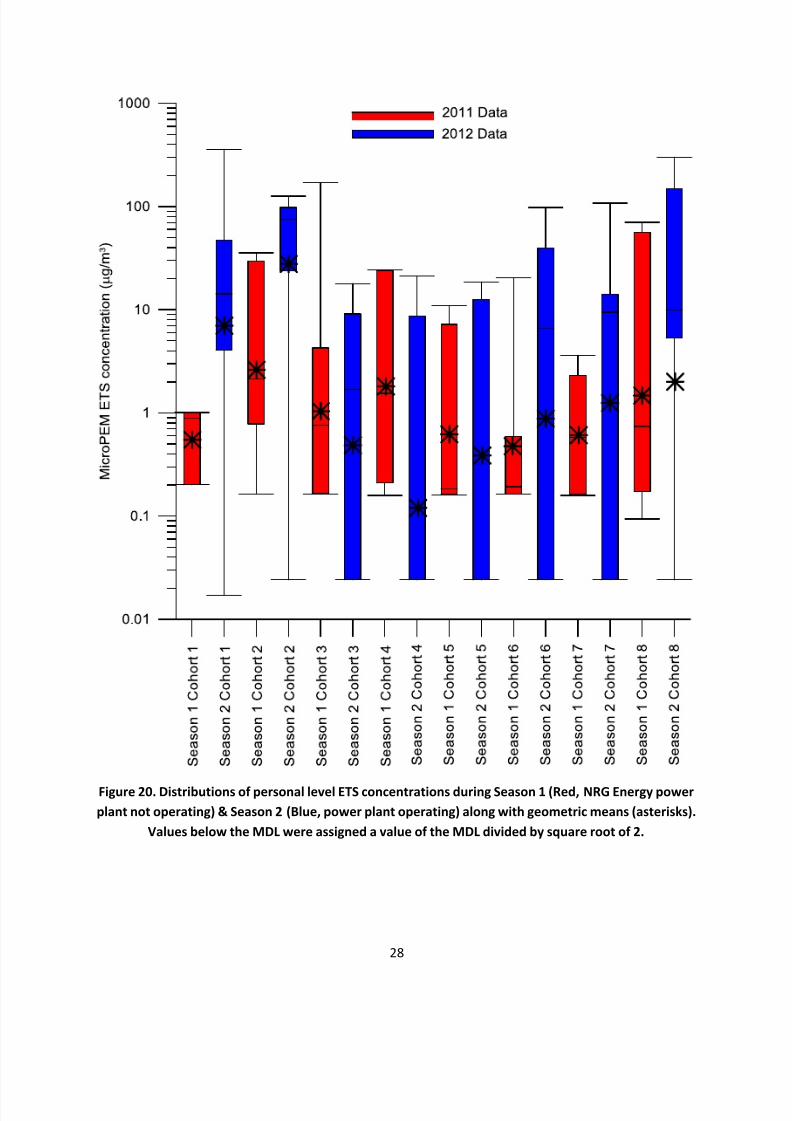
The high personal level concentrations are primarily driven by ETS exposure. Examination of

individual level data supports this conclusion. Of the 20 participants during Season 1 whose personal

exposure levels were in excess of the Federal 24 hour PM2.5 standard of 35 µg/m3, 65% of them were

also within the top 20 participants in terms of ETS concentration. This percentage increased during

Season 2, where 89% of the top 18 participants in terms of ETS exposure also had personal PM2.5

exposure levels in excess of 35 µg/m3. Therefore, although ETS concentrations averaged 1.0 ± SD 7.5

µg/m3 for Season 1 and 2.1 ± SD 31.3 µg/m3 during Season 2, they accounted for the vast majority of

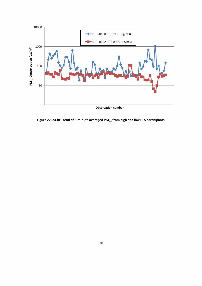
samples with elevated PM2.5 concentrations. To further illustrate the impact of ETS on personal

exposure, Figure 22 compares real-time PM2.5

acquired with the MicroPEM nephelometer from a

participant with high ETS concentrations to that of a participant with low ETS concentrations. The

household with high ETS tended to have a higher background concentration and several spikes in PM2.5

mass were observed. These spikes are thought to be due to the passive combustion and extinguishing of

cigarettes, an act which leads to large amounts of PM2.5, however without questionnaire data indicating

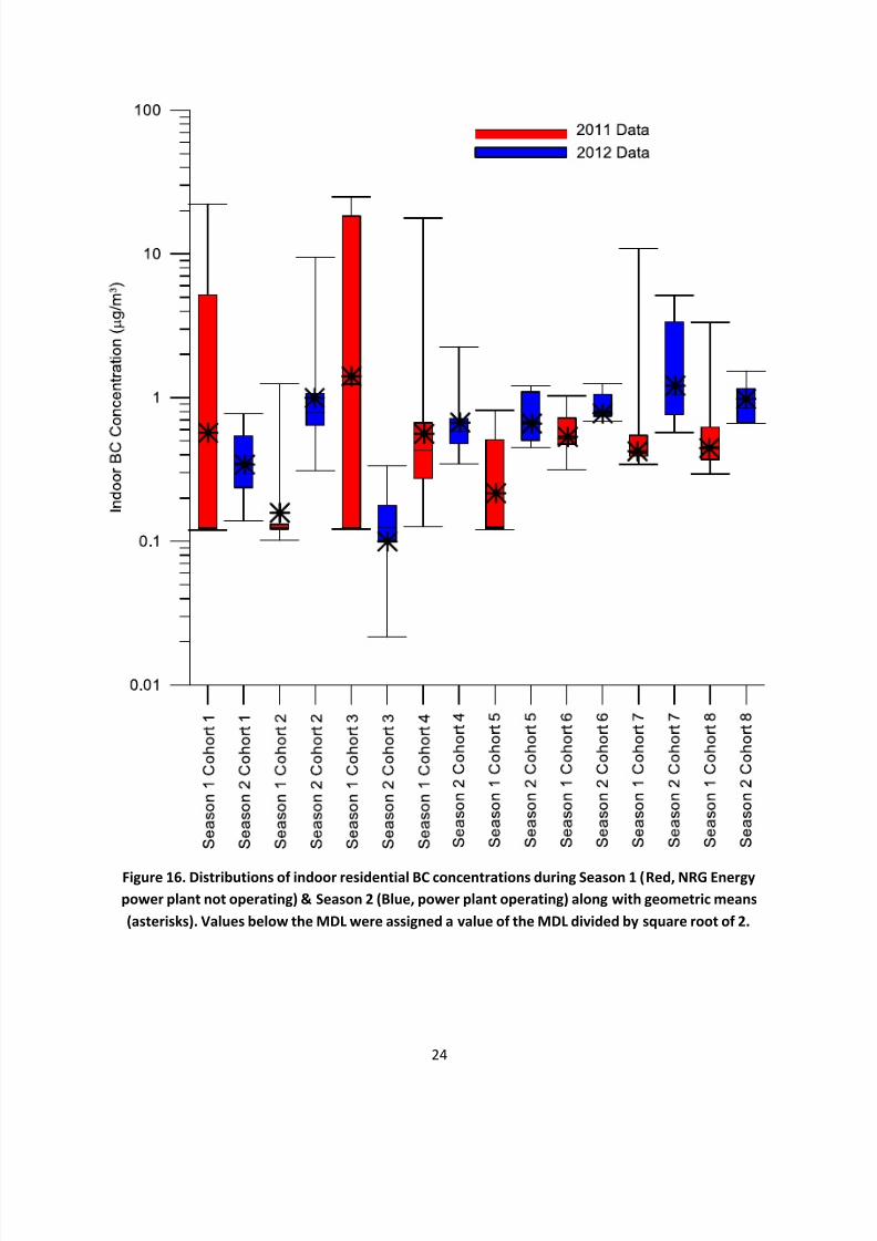
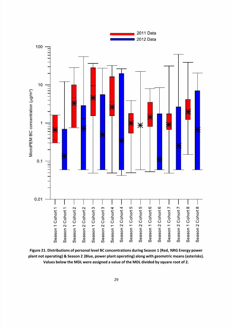
the presence of smokers within households, a definitive correlation cannot be determined. Black carbon

plays a lesser role in terms of the overall mass concentration of personal exposure than does ETS with



27

Figure 19. Distributions of personal level PM2.5 concentrations during Season 1 (Red, NRG Energy





28

Figure 20. Distributions of personal level ETS concentrations during Season 1 (Red, NRG Energy power





29

Figure 21. Distributions of personal level BC concentrations during Season 1 (Red, NRG Energy power





30

Figure 22. 24-hr Trend of 5-minute averaged PM2.5 from high and low ETS participants.

1

10

100

1000

10000

P M 2 . 5

C o n c e n t r a t i o n ( µ g / m

3 )

Observation number

DUP-0108 (ETS 59.78 µg/m3)

DUP-0102 (ETS 0.676 µg/m3)



31

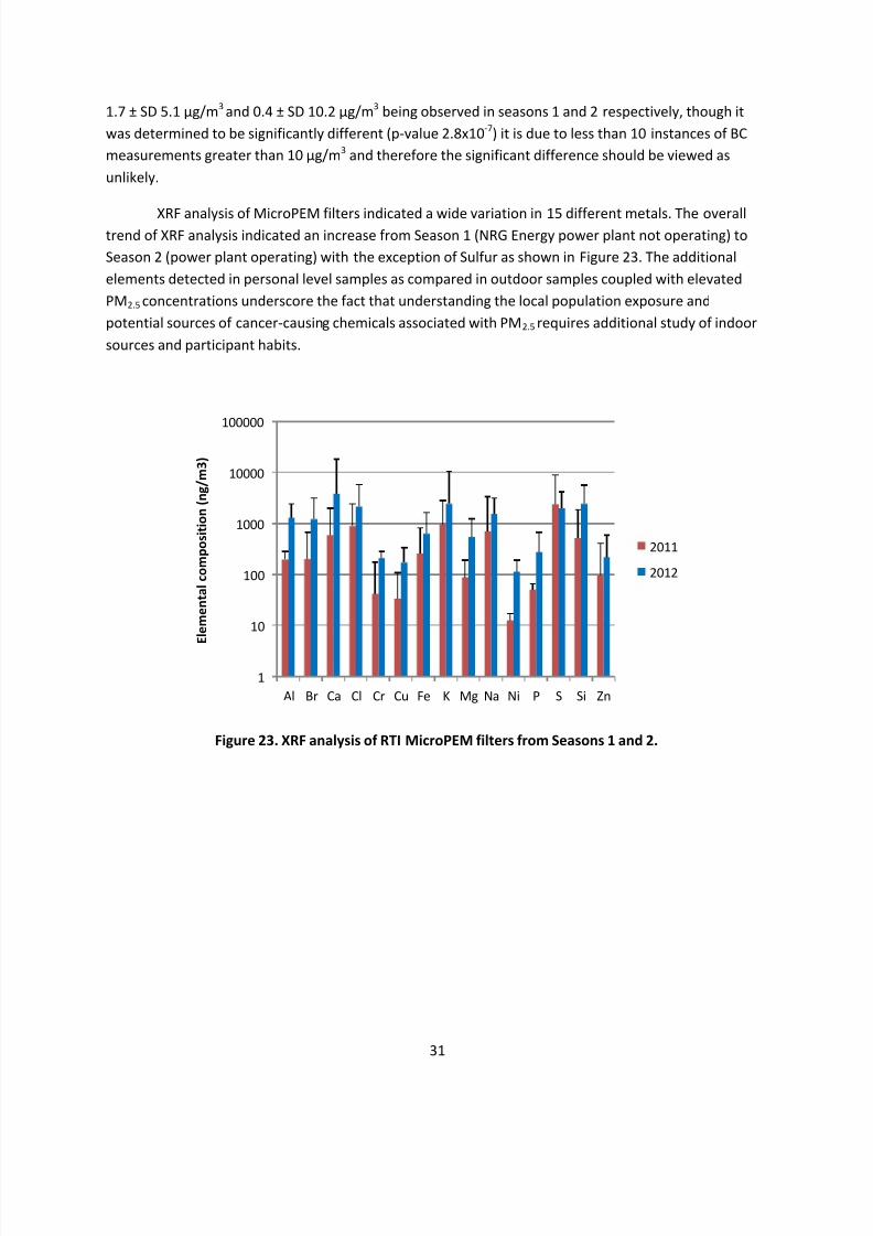
1.7 ± SD 5.1 µg/m3 and 0.4 ± SD 10.2 µg/m3 being observed in seasons 1 and 2 respectively, though it

was determined to be significantly different (p-value 2.8x10-7) it is due to less than 10 instances of BC

measurements greater than 10 µg/m3 and therefore the significant difference should be viewed as

unlikely.

XRF analysis of MicroPEM filters indicated a wide variation in 15 different metals. The overalltrend of XRF analysis indicated an increase from Season 1 (NRG Energy power plant not operating) to

Season 2 (power plant operating) with the exception of Sulfur as shown in Figure 23. The additional

elements detected in personal level samples as compared in outdoor samples coupled with elevated

PM2.5 concentrations underscore the fact that understanding the local population exposure and

potential sources of cancer-causing chemicals associated with PM2.5 requires additional study of indoor

sources and participant habits.

Figure 23. XRF analysis of RTI MicroPEM filters from Seasons 1 and 2.

1

10

100

1000

10000

100000

Al Br Ca Cl Cr Cu Fe K Mg Na Ni P S Si Zn

E l e m e n t a l c o m p o s i t i o n ( n g / m 3 )

2011

2012



32

Residential Temperature and Humidity

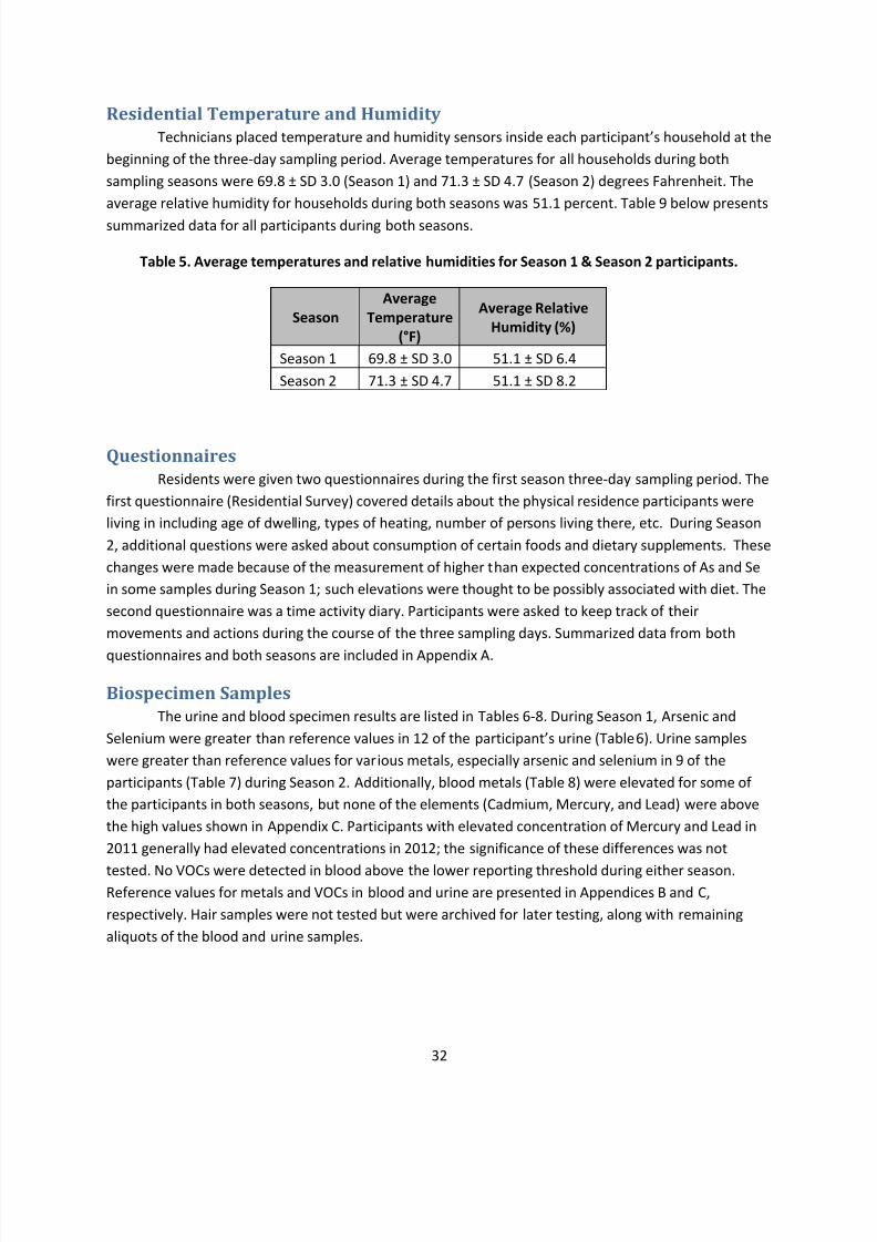
Technicians placed temperature and humidity sensors inside each participant’s household at the

beginning of the three-day sampling period. Average temperatures for all households during both

sampling seasons were 69.8 ± SD 3.0 (Season 1) and 71.3 ± SD 4.7 (Season 2) degrees Fahrenheit. The

average relative humidity for households during both seasons was 51.1 percent. Table 9 below presents

summarized data for all participants during both seasons.

Table 5. Average temperatures and relative humidities for Season 1 & Season 2 participants.

Season

Average

Temperature

(°F)

Average Relative

Humidity (%)

Season 1 69.8 ± SD 3.0 51.1 ± SD 6.4

Season 2 71.3 ± SD 4.7 51.1 ± SD 8.2

Questionnaires

Residents were given two questionnaires during the first season three-day sampling period. The

first questionnaire (Residential Survey) covered details about the physical residence participants were

living in including age of dwelling, types of heating, number of persons living there, etc. During Season

2, additional questions were asked about consumption of certain foods and dietary supplements. These

changes were made because of the measurement of higher than expected concentrations of As and Se

in some samples during Season 1; such elevations were thought to be possibly associated with diet. The

second questionnaire was a time activity diary. Participants were asked to keep track of their

movements and actions during the course of the three sampling days. Summarized data from both

questionnaires and both seasons are included in Appendix A.

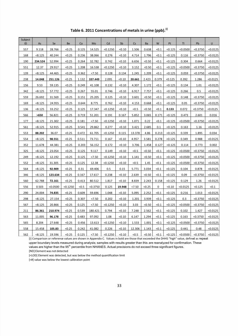
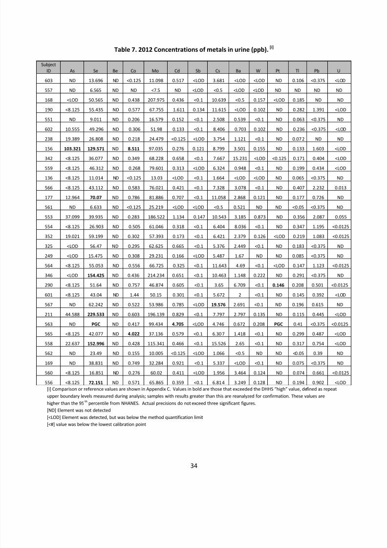
Biospecimen Samples

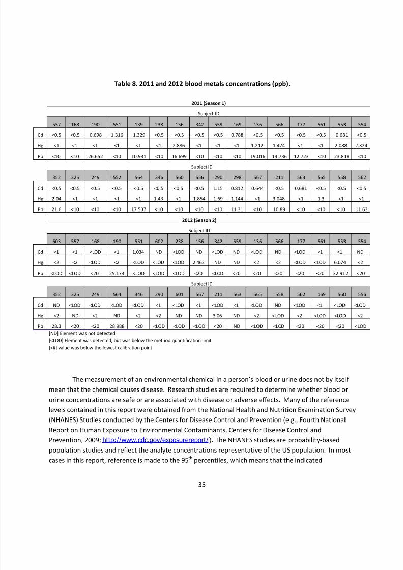
The urine and blood specimen results are listed in Tables 6-8. During Season 1, Arsenic and

Selenium were greater than reference values in 12 of the participant’s urine (Table6). Urine samples

were greater than reference values for various metals, especially arsenic and selenium in 9 of the

participants (Table 7) during Season 2. Additionally, blood metals (Table 8) were elevated for some of

the participants in both seasons, but none of the elements (Cadmium, Mercury, and Lead) were above

the high values shown in Appendix C. Participants with elevated concentration of Mercury and Lead in

2011 generally had elevated concentrations in 2012; the significance of these differences was not

tested. No VOCs were detected in blood above the lower reporting threshold during either season.Reference values for metals and VOCs in blood and urine are presented in Appendices B and C,

respectively. Hair samples were not tested but were archived for later testing, along with remaining

aliquots of the blood and urine samples.



33

Table 6. 2011 Concentrations of metals in urine (ppb).[i]

Subject

ID As Se Be Co Mo Cd Sb Cs Ba W Pt Tl Pb U

557 9.118 28.766 <0.25 0.125 14.525 <0.1250 <0.10 1.506 0.638 <0.1 <0.125 <0.0500 <0.3750 <0.0125

168 <8.125 40.244 <0.25 0.236 38.066 0.276 <0.10 4.714 1.796 <0.1 <0.125 0.116 <0.3750 <0.0125

190 234.524 52.994 <0.25 0.264 32.782 0.742 <0.10 6.656 <0.50 <0.1 <0.125 0.304 0.664 <0.0125

551 12.37 29.917 <0.25 1.208 16.538 <0.1250 <0.10 3.152 <0.50 <0.1 <0.125 <0.0500 <0.3750 <0.0125

139 <8.125 44.465 <0.25 0.362 <7.50 0.128 0.134 1.245 1.209 <0.1 <0.125 0.059 <0.3750 <0.0125

238 14.048 251.126 <0.25 1.132 337.449 2.095 <0.10 20.661 2.423 0.379 <0.125 0.392 1.286 <0.0125

156 9.53 59.135 <0.25 0.249 41.108 0.132 <0.10 4.307 1.172 <0.1 <0.125 0.134 1.01 <0.0125

342 <8.125 57.772 <0.25 0.267 55.01 0.746 <0.10 6.917 7.757 <0.1 <0.125 0.266 0.5 <0.0125

559 26.692 31.569 <0.25 0.151 25.205 0.125 <0.10 3.601 <0.50 <0.1 <0.125 0.148 <0.3750 <0.0125

169 <8.125 24.955 <0.25 0.644 8.775 0.762 <0.10 4.153 0.668 <0.1 <0.125 0.05 <0.3750 <0.0125

136 <8.125 33.252 <0.25 0.125 17.347 <0.1250 <0.10 <0.5 <0.50 <0.1 0.133 0.072 <0.3750 <0.0125

566 >650 56.821 <0.25 0.719 51.201 0.191 0.167 5.852 3.065 0.171 <0.125 0.473 2.601 0.016

177 <8.125 21.302 <0.25 0.181 <7.50 <0.1250 <0.10 1.071 0.22 <0.1 <0.125 <0.0500 <0.3750 <0.0125

561 <8.125 52.915 <0.25 0.541 29.862 0.277 <0.10 3.421 2.685 0.1 <0.125 0.163 1.16 <0.0125

553 88.202 36.07 <0.25 0.472 61.705 <0.1250 0.115 13.378 4.86 0.213 <0.125 0.339 1.895 0.034

554 <8.125 98.551 <0.25 0.511 73.711 0.167 <0.10 4.957 3.581 0.278 <0.125 0.349 0.988 <0.0125

352 11.678 44.381 <0.25 0.203 56.152 0.172 <0.10 3.706 1.458 0.127 <0.125 0.114 0.773 0.002

325 <8.125 23.054 <0.25 0.125 9.117 0.149 <0.10 <0.5 <0.50 <0.1 <0.125 <0.0500 <0.3750 <0.0125

249 <8.125 12.192 <0.25 0.125 <7.50 <0.1250 <0.10 1.141 <0.50 <0.1 <0.125 <0.0500 <0.3750 <0.0125

552 <8.125 31.305 <0.25 0.125 12.38 <0.1250 <0.10 <0.5 1.45 <0.1 <0.125 <0.0500 <0.3750 <0.0125

564 <8.125 92.909 <0.25 0.31 69.406 0.5 0.15 5.771 3.034 <0.1 <0.125 0.104 0.878 <0.0125

346 <8.125 123.634 <0.25 0.167 17.617 0.238 <0.10 2.639 <0.50 <0.1 <0.125 0.09 <0.3750 <0.0125

560 62.788 72.161 <0.25 0.413 80.512 1.817 <0.10 8.839 2.243 0.158 <0.125 0.129 1.26 <0.0125

556 0.503 <0.0500 <0.1250 <0.5 <0.3750 0.125 19.948 <7.50 <0.25 0 <0.10 <0.0125 <0.125 <0.1

290 24.004 74.835 <0.25 0.609 59.696 1.048 <0.10 5.095 2.252 <0.1 <0.125 0.216 1.013 <0.0125

298 <8.125 27.154 <0.25 0.307 <7.50 0.202 <0.10 1.201 3.939 <0.1 <0.125 0.3 <0.3750 <0.0125

567 <8.125 20.866 <0.25 0.125 <7.50 <0.1250 <0.10 3.03 <0.50 <0.1 <0.125 <0.0500 <0.3750 <0.0125

211 86.361 210.974 <0.25 0.539 180.421 0.794 <0.10 7.248 2.562 <0.1 <0.125 0.102 1.427 <0.0125

563 11.005 96.178 <0.25 0.483 97.092 1.08 <0.10 6.147 1.294 <0.1 <0.125 0.163 <0.3750 <0.0125

565 8.204 27.648 <0.25 0.456 13.613 <0.1250 <0.10 1.533 1.001 <0.1 <0.125 <0.0500 <0.3750 <0.0125

558 15.458 105.83 <0.25 0.242 41.082 0.226 <0.10 12.306 1.143 <0.1 <0.125 0.441 0.48 <0.0125

562 <8.125 19.596 <0.25 0.125 <7.50 <0.1250 <0.10 <0.5 <0.50 <0.1 <0.125 <0.0500 <0.3750 <0.0125[i] Comparison or reference values are shown in Appendix C. Values in bold are those that exceeded the DHHS “high” value, defined as repeat

upper boundary levels measured during analysis; samples with results greater than this are reanalyzed for confirmation. These

values are higher than the 95th

percentile from NHANES. Actual precisions do not exceed three significant figures.

[ND] Element was not detected

[<LOD] Element was detected, but was below the method quantification limit

[<#] value was below the lowest calibration point



34

Table 7. 2012 Concentrations of metals in urine (ppb). [i]

Subject

ID As Se Be Co Mo Cd Sb Cs Ba W Pt Tl Pb U

603 ND 13.696 ND <0.125 11.098 0.517 <LOD 3.681 <LOD <LOD ND 0.106 <0.375 <LOD

557 ND 6.565 ND ND <7.5 ND <LOD <0.5 <LOD <LOD ND ND ND ND

168 <LOD 50.565 ND 0.438 207.975 0.436 <0.1 10.639 <0.5 0.157 <LOD 0.185 ND ND

190 <8.125 55.435 ND 0.577 67.755 1.611 0.134 11.615 <LOD 0.102 ND 0.282 1.391 <LOD

551 ND 9.011 ND 0.206 16.579 0.152 <0.1 2.508 0.539 <0.1 ND 0.063 <0.375 ND

602 10.555 49.296 ND 0.306 51.98 0.133 <0.1 8.406 0.703 0.102 ND 0.236 <0.375 <LOD

238 19.389 26.808 ND 0.218 24.479 <0.125 <LOD 3.754 1.121 <0.1 ND 0.072 ND ND

156 103.321 129.571 ND 8.511 97.035 0.276 0.121 8.799 3.501 0.155 ND 0.133 1.603 <LOD

342 <8.125 36.077 ND 0.349 68.228 0.658 <0.1 7.667 15.231 <LOD <0.125 0.171 0.404 <LOD

559 <8.125 46.312 ND 0.268 79.601 0.313 <LOD 6.324 0.948 <0.1 ND 0.199 0.434 <LOD

136 <8.125 11.014 ND <0.125 13.03 <LOD <0.1 1.664 <LOD <LOD ND 0.065 <0.375 ND

566 <8.125 43.112 ND 0.583 76.021 0.421 <0.1 7.328 3.078 <0.1 ND 0.407 2.232 0.013

177 12.964 70.07 ND 0.786 81.886 0.707 <0.1 11.058 2.868 0.121 ND 0.177 0.726 ND

561 ND 6.633 ND <0.125 25.219 <LOD <LOD <0.5 0.521 ND ND <0.05 <0.375 ND

553 37.099 39.935 ND 0.283 186.522 1.134 0.147 10.543 3.185 0.873 ND 0.356 2.087 0.055

554 <8.125 26.903 ND 0.505 61.046 0.318 <0.1 6.404 8.036 <0.1 ND 0.347 1.195 <0.0125

352 19.021 59.199 ND 0.302 57.393 0.173 <0.1 6.421 2.379 0.126 <LOD 0.219 1.083 <0.0125

325 <LOD 56.47 ND 0.295 62.625 0.665 <0.1 5.376 2.449 <0.1 ND 0.183 <0.375 ND

249 <LOD 15.475 ND 0.308 29.231 0.166 <LOD 5.487 1.67 ND ND 0.085 <0.375 ND

564 <8.125 55.053 ND 0.556 66.725 0.325 <0.1 11.643 4.69 <0.1 <LOD 0.147 1.123 <0.0125

346 <LOD 154.425 ND 0.436 214.234 0.651 <0.1 10.463 1.148 0.222 ND 0.291 <0.375 ND

290 <8.125 51.64 ND 0.757 46.874 0.605 <0.1 3.65 6.709 <0.1 0.146 0.208 0.501 <0.0125

601 <8.125 43.04 ND 1.44 50.15 0.301 <0.1 5.672 2 <0.1 ND 0.145 0.392 <LOD

567 ND 62.242 ND 0.522 53.986 0.785 <LOD 19.576 2.691 <0.1 ND 0.196 0.615 ND

211 44.588 229.533 ND 0.603 196.139 0.829 <0.1 7.797 2.797 0.135 ND 0.115 0.445 <LOD

563 ND PGC ND 0.417 99.434 4.705 <LOD 4.746 0.672 0.208 PGC 0.41 <0.375 <0.0125

565 <8.125 42.077 ND 4.022 37.136 0.579 <0.1 6.307 1.418 <0.1 ND 0.299 0.487 <LOD

558 22.637 152.996 ND 0.428 115.341 0.466 <0.1 15.526 2.65 <0.1 ND 0.317 0.754 <LOD

562 ND 23.49 ND 0.155 10.005 <0.125 <LOD 1.066 <0.5 ND ND <0.05 0.39 ND

169 ND 38.831 ND 0.749 32.284 0.921 <0.1 5.337 <LOD <0.1 ND 0.075 <0.375 ND

560 <8.125 16.851 ND 0.276 60.02 0.411 <LOD 1.956 3.464 0.124 ND 0.074 0.661 <0.0125

556 <8.125 72.151 ND 0.571 65.865 0.359 <0.1 6.814 3.249 0.128 ND 0.194 0.902 <LOD[i] Comparison or reference values are shown in Appendix C. Values in bold are those that exceeded the DHHS “high” value, defined as repeat

upper boundary levels measured during analysis; samples with results greater than this are reanalyzed for confirmation. These values are

higher than the 95th

percentile from NHANES. Actual precisions do not exceed three significant figures.






35

Table 8. 2011 and 2012 blood metals concentrations (ppb).

2011 (Season 1)

Subject ID

557 168 190 551 139 238 156 342 559 169 136 566 177 561 553 554

Cd <0.5 <0.5 0.698 1.316 1.329 <0.5 <0.5 <0.5 <0.5 0.788 <0.5 <0.5 <0.5 <0.5 0.681 <0.5

Hg <1 <1 <1 <1 <1 <1 2.886 <1 <1 <1 1.212 1.474 <1 <1 2.088 2.324

Pb <10 <10 26.652 <10 10.931 <10 16.699 <10 <10 <10 19.016 14.736 12.723 <10 23.818 <10

Subject ID

352 325 249 552 564 346 560 556 290 298 567 211 563 565 558 562

Cd <0.5 <0.5 <0.5 <0.5 <0.5 <0.5 <0.5 <0.5 1.15 0.812 0.644 <0.5 0.681 <0.5 <0.5 <0.5

Hg 2.04 <1 <1 <1 <1 1.43 <1 1.854 1.69 1.144 <1 3.048 <1 1.3 <1 <1

Pb 21.6 <10 <10 <10 17.537 <10 <10 <10 <10 11.31 <10 10.89 <10 <10 <10 11.63

2012 (Season 2)

Subject ID

603 557 168 190 551 602 238 156 342 559 136 566 177 561 553 554

Cd <1 <1 <LOD <1 1.034 ND <LOD ND <LOD ND <LOD ND <LOD <1 <1 ND

Hg <2 <2 <LOD <2 <LOD <LOD <LOD 2.462 ND ND <2 <2 <LOD <LOD 6.074 <2

Pb <LOD <LOD <20 25.173 <LOD <LOD <LOD <20 <LOD <20 <20 <20 <20 <20 32.912 <20

Subject ID

352 325 249 564 346 290 601 567 211 563 565 558 562 169 560 556

Cd ND <LOD <LOD <LOD <LOD <1 <LOD <1 <LOD <1 <LOD ND <LOD <1 <LOD <LOD

Hg <2 ND <2 ND <2 <2 ND ND 3.06 ND <2 <LOD <2 <LOD <LOD <2

Pb 28.3 <20 <20 28.988 <20 <LOD <LOD <LOD <20 ND <LOD <LOD <20 <20 <20 <LOD




The measurement of an environmental chemical in a person’s blood or urine does not by itself

mean that the chemical causes disease. Research studies are required to determine whether blood or

urine concentrations are safe or are associated with disease or adverse effects. Many of the referencelevels contained in this report were obtained from the National Health and Nutrition Examination Survey

(NHANES) Studies conducted by the Centers for Disease Control and Prevention (e.g., Fourth National

Report on Human Exposure to Environmental Contaminants, Centers for Disease Control and

Prevention, 2009; http://www.cdc.gov/exposurereport/). The NHANES studies are probability-based

population studies and reflect the analyte concentrations representative of the US population. In most

cases in this report, reference is made to the 95th percentiles, which means that the indicated

http://www.cdc.gov/exposurereport/






36

concentrations are equal to or higher than those measured for 95% of the population. This value is

useful for determining whether or not a concentration measured in any particular public health study is

unusual. The reader is encouraged to visit the website shown above for more information about many

of the analytes measured.

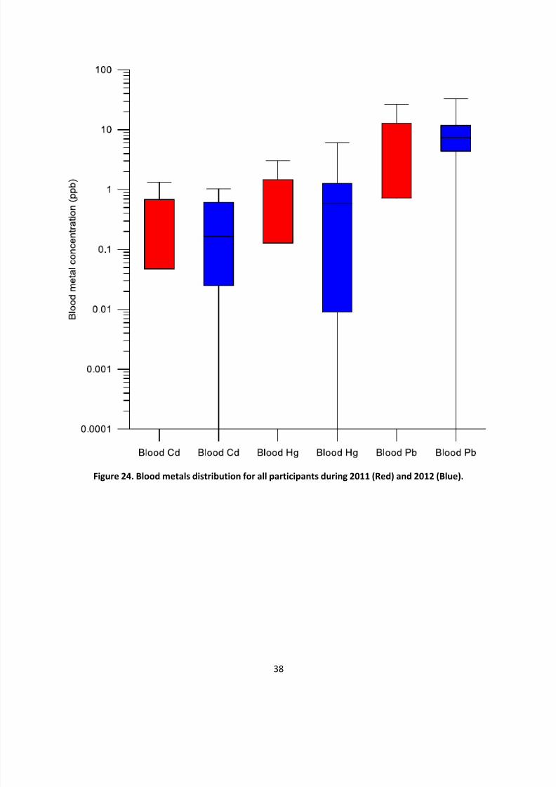
Distributions of the biospecimen results for each season are shown below for blood (Figure 24)and for urine (Figure 25) for both seasons. Note that for these results, values below MDL or those that

were not detected were reported as 0.5 times the limit of detection. On average, there do not appear to

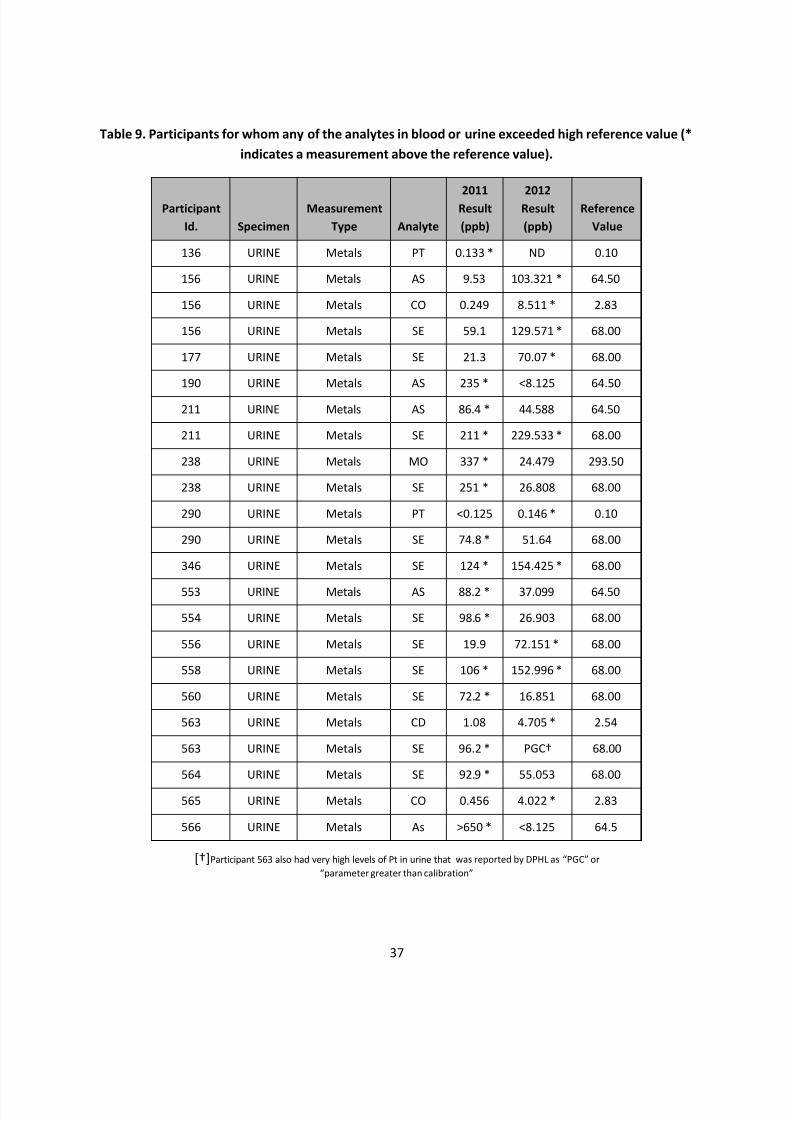
be any significant changes across seasons. However, several participants had concentrations that

exceeded the high reference value for various elements in one or both seasons (Table 9). By far the

most common exceedances were for Arsenic and Selenium. For those 2012 participants with urinary

concentrations of As or Se that were above the high reference values, we evaluated their responses to

the dietary questions added for the 2012 sampling season. Participant 156 consumed locally caught fish

(tautog), ate meat, poultry, and locally-grown produce on a on a regular basis but did not report taking

any multivitamins or Selenium containing supplements. Those participants with elevated concentrations

of Se only (346, 211. 558, and 556) reported regular consumption of meats, poultry, grains, and localproduce. Participants 346, 211, 558, and 556 all took multivitamins with participants 211 and 556

reporting taking a fish oil supplement. A key parameter in evaluation of the effect of these actions on

urinary metals concentrations is the time between providing a urine sample and consumption. In the

case of grains and local seafood, these actions were taken within the past 48 hours of providing a urine

sample; therefore the linkage between these actions is potentially stronger than those actions with no

time-related information.

An important component of this study was to evaluate how exposure to particulate matter is

associated with measures from the biospecimens. Measured PM permitted evaluation of four

characteristics: mass, ETS, Black carbon, and elemental composition. Relationships of each PM measureto each analyte/matrix combination in the biospecimens were examined. PM measurement

characteristics were averaged over the course of the three day sampling period since there was only one

biospecimen data point to reflect each participant. Non-ranked correlations were performed with the

following tables indicating how predictive each PM characteristic was for each biospecimen analyte. The

scatter plots were examined to ensure that the correlation was not being driven by a single extreme

value.

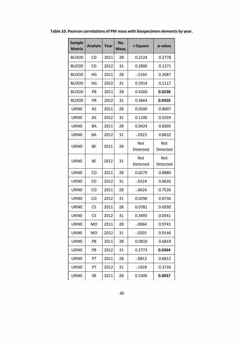
Table 10 shows the results for PM mass to be predictive of elements in blood and urine. Blood

lead appears to be associated with PM mass each year, but it is also persistent in the body. Table 11

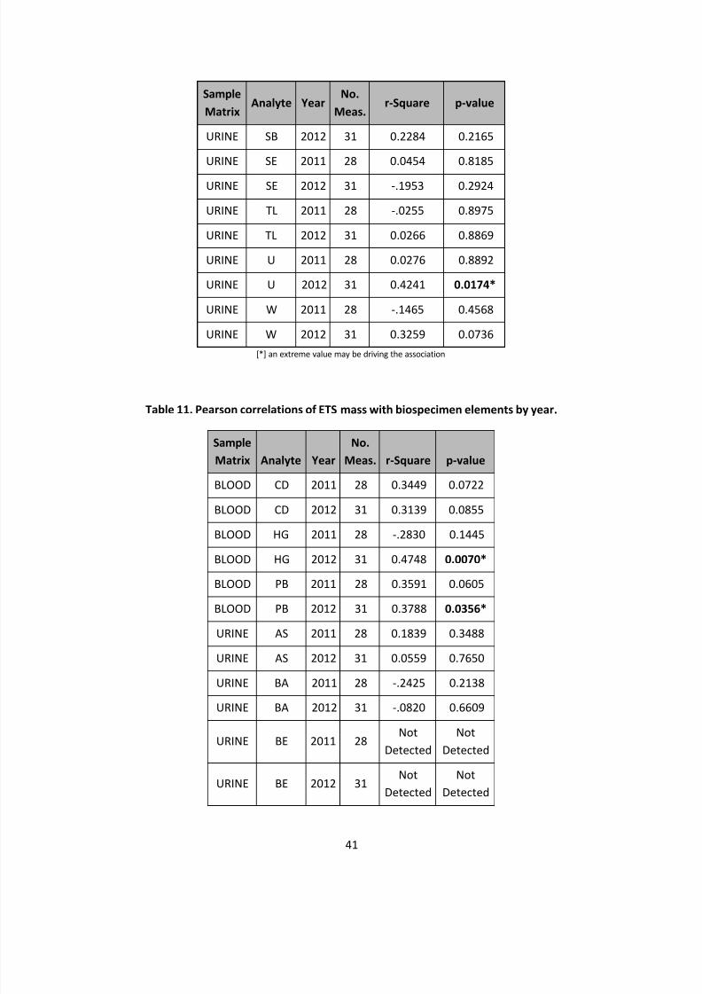
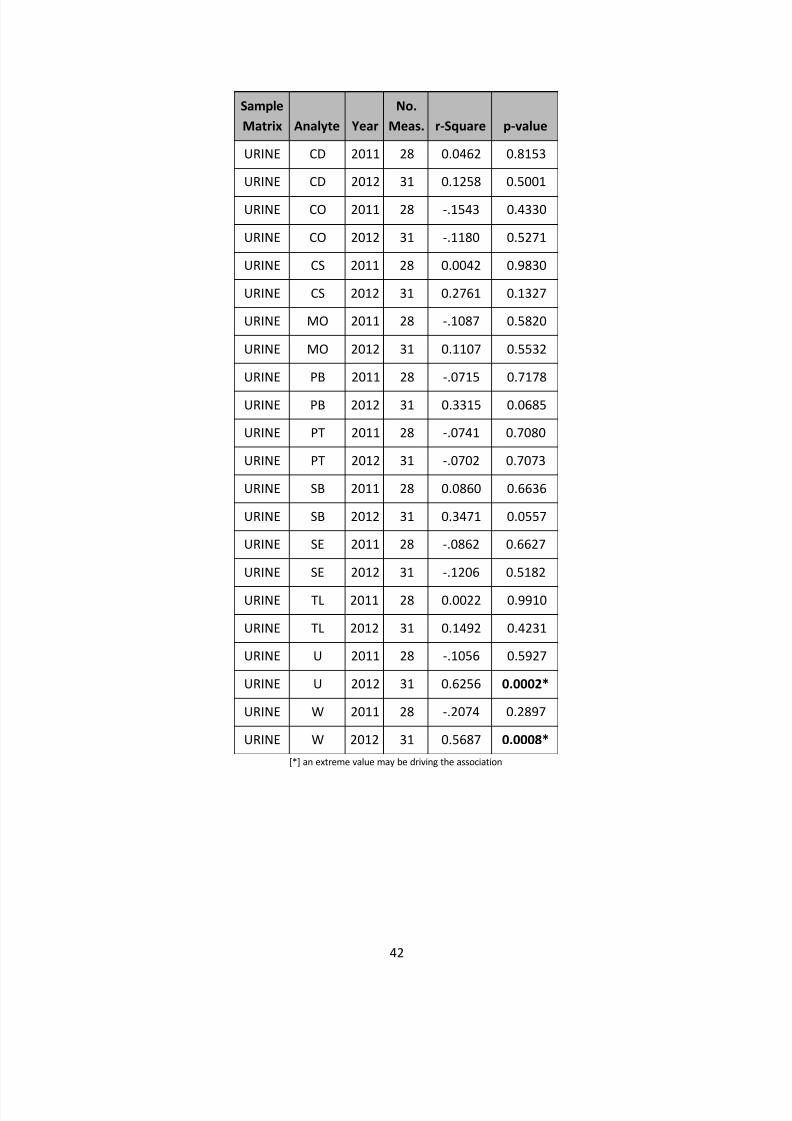
shows the correlation of ETS with elements in blood and urine. Although significance was found for

blood mercury, blood lead, and urinary uranium, all of these appeared to be driven by a single, high

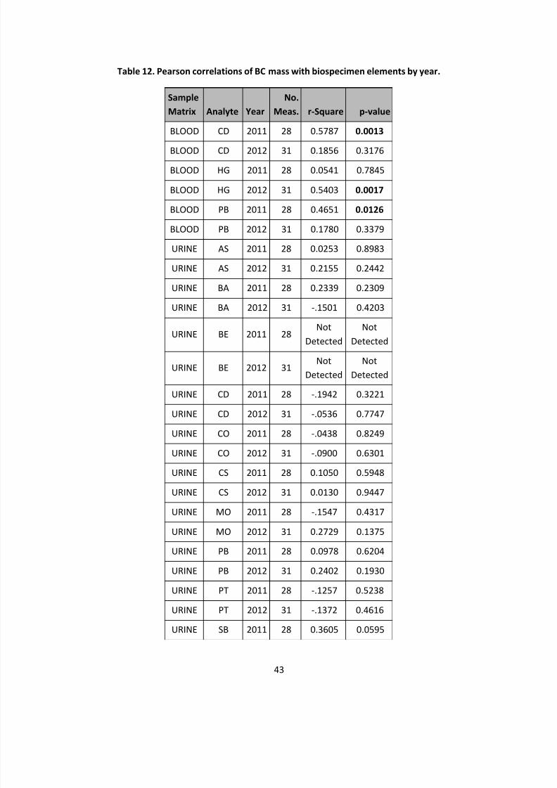
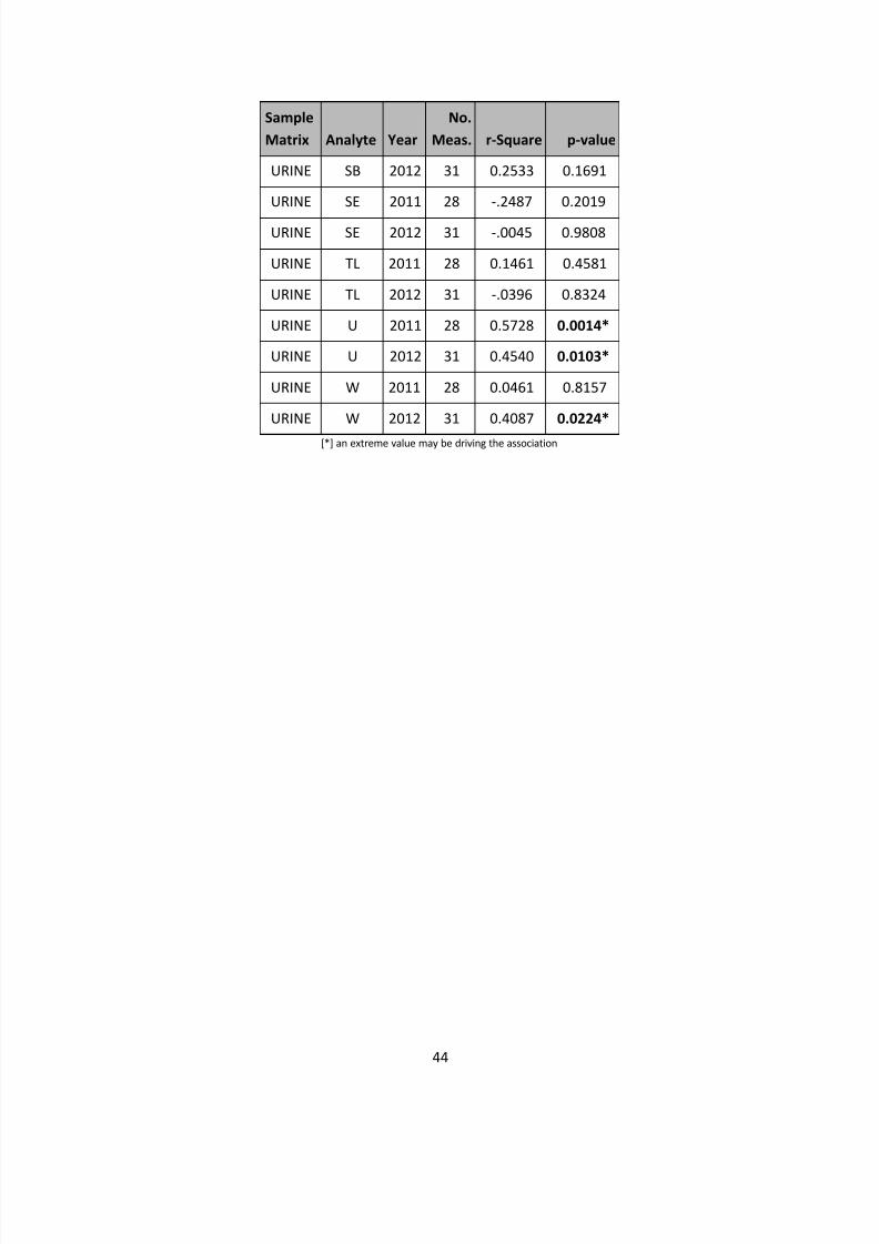
value. Table 12 shows associations of BC with elements in blood and urine. P-values <0.05 were found

for blood Cd and Pb in 2011 and blood Hg in 2012; other significant associations were clearly driven by

extreme values and should not be believed. In general, some associations were observed between some

elements with total mass, ETS, and BC, but they were not consistent across all elements or across the

two years of the study.



37

Table 9. Participants for whom any of the analytes in blood or urine exceeded high reference value (*

indicates a measurement above the reference value).

[†]Participant 563 also had very high levels of Pt in urine that was reported by DPHL as “PGC” or

“parameter greater than calibration”

Participant

Id. Specimen

Measurement

Type Analyte

2011Result

(ppb)

2012Result

(ppb)

Reference

Value

136 URINE Metals PT 0.133 * ND 0.10

156 URINE Metals AS 9.53 103.321 * 64.50

156 URINE Metals CO 0.249 8.511 * 2.83

156 URINE Metals SE 59.1 129.571 * 68.00

177 URINE Metals SE 21.3 70.07 * 68.00

190 URINE Metals AS 235 * <8.125 64.50

211 URINE Metals AS 86.4 * 44.588 64.50

211 URINE Metals SE 211 * 229.533 * 68.00

238 URINE Metals MO 337 * 24.479 293.50

238 URINE Metals SE 251 * 26.808 68.00

290 URINE Metals PT <0.125 0.146 * 0.10

290 URINE Metals SE 74.8 * 51.64 68.00

346 URINE Metals SE 124 * 154.425 * 68.00

553 URINE Metals AS 88.2 * 37.099 64.50

554 URINE Metals SE 98.6 * 26.903 68.00

556 URINE Metals SE 19.9 72.151 * 68.00

558 URINE Metals SE 106 * 152.996 * 68.00

560 URINE Metals SE 72.2 * 16.851 68.00

563 URINE Metals CD 1.08 4.705 * 2.54

563 URINE Metals SE 96.2 * PGC† 68.00

564 URINE Metals SE 92.9 * 55.053 68.00

565 URINE Metals CO 0.456 4.022 * 2.83

566 URINE Metals As >650 * <8.125 64.5



38

Figure 24. Blood metals distribution for all participants during 2011 (Red) and 2012 (Blue).



39

Figure 25. Urine metals distributions for all participants during 2011 (Red) and 2012 (Blue).



40

Table 10. Pearson correlations of PM mass with biospecimen elements by year.

Sample

MatrixAnalyte Year

No.

Meas.r-Square p-value

BLOOD CD 2011 28 0.2124 0.2778

BLOOD CD 2012 31 0.2800 0.1271

BLOOD HG 2011 28 -.2164 0.2687

BLOOD HG 2012 31 0.2914 0.1117

BLOOD PB 2011 28 0.4260 0.0238

BLOOD PB 2012 31 0.3664 0.0426

URINE AS 2011 28 0.0500 0.8007

URINE AS 2012 31 0.1100 0.5559

URINE BA 2011 28 0.0424 0.8305

URINE BA 2012 31 -.0323 0.8632

URINE BE 2011 28Not

Detected

Not

Detected

URINE BE 2012 31Not

Detected

Not

Detected

URINE CD 2011 28 0.0279 0.8880

URINE CD 2012 31 -.0324 0.8626

URINE CO 2011 28 -.0624 0.7526

URINE CO 2012 31 0.0298 0.8736

URINE CS 2011 28 0.0781 0.6930

URINE CS 2012 31 0.3493 0.0541

URINE MO 2011 28 -.0064 0.9741

URINE MO 2012 31 -.0201 0.9146

URINE PB 2011 28 0.0810 0.6819

URINE PB 2012 31 0.3773 0.0364

URINE PT 2011 28 -.0812 0.6812

URINE PT 2012 31 -.1659 0.3726

URINE SB 2011 28 0.5306 0.0037



41

Sample

MatrixAnalyte Year

No.

Meas.r-Square p-value

URINE SB 2012 31 0.2284 0.2165

URINE SE 2011 28 0.0454 0.8185

URINE SE 2012 31 -.1953 0.2924

URINE TL 2011 28 -.0255 0.8975

URINE TL 2012 31 0.0266 0.8869

URINE U 2011 28 0.0276 0.8892

URINE U 2012 31 0.4241 0.0174*

URINE W 2011 28 -.1465 0.4568

URINE W 2012 31 0.3259 0.0736

[*] an extreme value may be driving the association

Table 11. Pearson correlations of ETS mass with biospecimen elements by year.

Sample

Matrix Analyte Year

No.

Meas. r-Square p-value

BLOOD CD 2011 28 0.3449 0.0722

BLOOD CD 2012 31 0.3139 0.0855

BLOOD HG 2011 28 -.2830 0.1445

BLOOD HG 2012 31 0.4748 0.0070*

BLOOD PB 2011 28 0.3591 0.0605

BLOOD PB 2012 31 0.3788 0.0356*

URINE AS 2011 28 0.1839 0.3488

URINE AS 2012 31 0.0559 0.7650

URINE BA 2011 28 -.2425 0.2138

URINE BA 2012 31 -.0820 0.6609

URINE BE 2011 28Not

Detected

Not

Detected

URINE BE 2012 31Not

Detected

Not

Detected



42

Sample

Matrix Analyte Year

No.


URINE CD 2011 28 0.0462 0.8153

URINE CD 2012 31 0.1258 0.5001

URINE CO 2011 28 -.1543 0.4330

URINE CO 2012 31 -.1180 0.5271

URINE CS 2011 28 0.0042 0.9830

URINE CS 2012 31 0.2761 0.1327

URINE MO 2011 28 -.1087 0.5820

URINE MO 2012 31 0.1107 0.5532

URINE PB 2011 28 -.0715 0.7178

URINE PB 2012 31 0.3315 0.0685

URINE PT 2011 28 -.0741 0.7080

URINE PT 2012 31 -.0702 0.7073

URINE SB 2011 28 0.0860 0.6636

URINE SB 2012 31 0.3471 0.0557

URINE SE 2011 28 -.0862 0.6627

URINE SE 2012 31 -.1206 0.5182

URINE TL 2011 28 0.0022 0.9910

URINE TL 2012 31 0.1492 0.4231

URINE U 2011 28 -.1056 0.5927

URINE U 2012 31 0.6256 0.0002*

URINE W 2011 28 -.2074 0.2897

URINE W 2012 31 0.5687 0.0008*




43

Table 12. Pearson correlations of BC mass with biospecimen elements by year.

Sample

Matrix Analyte Year

No.


BLOOD CD 2011 28 0.5787 0.0013

BLOOD CD 2012 31 0.1856 0.3176

BLOOD HG 2011 28 0.0541 0.7845

BLOOD HG 2012 31 0.5403 0.0017

BLOOD PB 2011 28 0.4651 0.0126

BLOOD PB 2012 31 0.1780 0.3379

URINE AS 2011 28 0.0253 0.8983

URINE AS 2012 31 0.2155 0.2442

URINE BA 2011 28 0.2339 0.2309

URINE BA 2012 31 -.1501 0.4203

URINE BE 2011 28Not

Detected

Not

Detected

URINE BE 2012 31Not

Detected

Not

Detected

URINE CD 2011 28 -.1942 0.3221

URINE CD 2012 31 -.0536 0.7747

URINE CO 2011 28 -.0438 0.8249

URINE CO 2012 31 -.0900 0.6301

URINE CS 2011 28 0.1050 0.5948

URINE CS 2012 31 0.0130 0.9447

URINE MO 2011 28 -.1547 0.4317

URINE MO 2012 31 0.2729 0.1375

URINE PB 2011 28 0.0978 0.6204

URINE PB 2012 31 0.2402 0.1930

URINE PT 2011 28 -.1257 0.5238

URINE PT 2012 31 -.1372 0.4616

URINE SB 2011 28 0.3605 0.0595



44

Sample

Matrix Analyte Year

No.


URINE SB 2012 31 0.2533 0.1691

URINE SE 2011 28 -.2487 0.2019

URINE SE 2012 31 -.0045 0.9808

URINE TL 2011 28 0.1461 0.4581

URINE TL 2012 31 -.0396 0.8324

URINE U 2011 28 0.5728 0.0014*

URINE U 2012 31 0.4540 0.0103*

URINE W 2011 28 0.0461 0.8157

URINE W 2012 31 0.4087 0.0224*




45

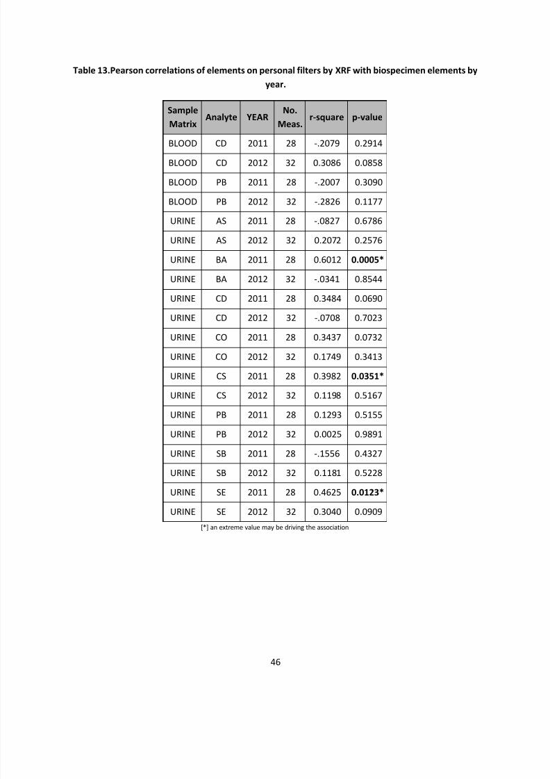
Lastly, a comparison was performed between the elemental concentrations measured of the

collected personal level PM2.5 to those measured in urine or blood. Table 13 indicates the associations of

elements on personal PM filters, as measured by XRF, to the same elements measured in biospecimen

samples by year, while Table 14 compares across both years of sampling. When examined by year, three

associations were identified, but they were all found to have been driven by one or a few extreme

values and are not predictive. No significant associations were observed when the data from both years

were combined.

It does not appear that the personal PM characteristics measured in this study have strong and

consistent contributions to the analytes measured in the blood and urine from the study participants.

The lack of relationship may mean that current exposures do not result in large biospecimen changes on

the time scale of this study. In other words, measures for some of the analytes in biospecimens might

reflect long-term equilibria that are not perturbed to any great extent by the short-term change in PM.

These data might also indicate the possibility of non-inhalation routes of exposure. When considering

the biospecimen analyte concentrations that exceeded reference values (Table 9), most of the

excursions are measured for Arsenic and Selenium, two elements known to have dietary sources.Exposure to these metals has health consequences that range from cancer to other less severe

consequences which depend on both exposure amount and length. As described earlier, questions were

added to the participant survey for Season 2 to examine some potential dietary sources.

Table 15 examines the relationship between elevated urinary concentrations of Arsenic and

Selenium and various ingestion sources. Specific potential contributors to individual excursions were

examined previously. The purpose of the correlations presented in Table 15 is an attempt to see how

generalizable the findings might be to the rest of the study participants, whether or not their particular

biospecimen results where high or more typical of this group. Some of the dependent variables in the

table are categorical, i.e., they have a “yes” or “no” response. Such variables include eating grains, localproduce, rice, or meat, drinking filtered water, taking dietary supplements, eating fish/seafood, or

whether a participant’s source of drinking water was a private well or municipal water supply. Another

factor to consider is the relative amount of time spent indoor versus outdoors. This would not be

expected to influence exposure to Arsenic or Selenium, unless there is an inhalation source (not

supported by the results shown above), but could for other pollutants. This was not explored further in

this work. In any event, the data show that the consumption of seafood within 48 hours of providing a

urinary sample is significantly linked to increased urinary Arsenic levels. It is important to recognize,

however, that this study measured total (inorganic + organic) arsenic in urine, while arsenic in fish is

predominantly organic arsenic (Greene and Crecelius, 2006). Inorganic arsenic is considered toxic, while

organic arsenic is not. Further, organic arsenic is quickly excreted from the body. Total urinary arsenicvalues can occasionally increase to several thousands of ug/L after seafood consumption (Caldwell et.

al., 2009), which is well above values seen in the current study. It is also important to note that arsenic

concentrations in fish and shellfish from the local Inland Bays are not greater than concentrations in fish

and shellfish from the entire East and Gulf Coasts of the U.S. (Greene, 2010). The data also suggest that

the regular consumption of grains significantly decreases exposure to Arsenic. The reason is not

immediately obvious, but could reflect associated dietary factors or food interactions.



46

Table 13.Pearson correlations of elements on personal filters by XRF with biospecimen elements by

year.

Sample

MatrixAnalyte YEAR

No.

Meas.r-square p-value

BLOOD CD 2011 28 -.2079 0.2914

BLOOD CD 2012 32 0.3086 0.0858

BLOOD PB 2011 28 -.2007 0.3090

BLOOD PB 2012 32 -.2826 0.1177

URINE AS 2011 28 -.0827 0.6786

URINE AS 2012 32 0.2072 0.2576

URINE BA 2011 28 0.6012 0.0005*

URINE BA 2012 32 -.0341 0.8544

URINE CD 2011 28 0.3484 0.0690

URINE CD 2012 32 -.0708 0.7023

URINE CO 2011 28 0.3437 0.0732

URINE CO 2012 32 0.1749 0.3413

URINE CS 2011 28 0.3982 0.0351*

URINE CS 2012 32 0.1198 0.5167

URINE PB 2011 28 0.1293 0.5155

URINE PB 2012 32 0.0025 0.9891

URINE SB 2011 28 -.1556 0.4327

URINE SB 2012 32 0.1181 0.5228

URINE SE 2011 28 0.4625 0.0123*

URINE SE 2012 32 0.3040 0.0909




47

Table 14. Pearson correlations of elements on personal filters by XRF with biospecimen elements

across years.

Sample

MatrixAnalyte

No.

Meas.r-square p-value

BLOOD CD 60 -.1596 0.2243

BLOOD PB 60 -.2048 0.1169

URINE AS 60 0.0001 0.9996

URINE BA 60 0.2411 0.0634

URINE CD 60 0.1024 0.4377

URINE CO 60 0.0027 0.9839

URINE CS 60 0.1561 0.2346

URINE PB 60 0.0688 0.6031

URINE SB 60 -.1323 0.3150

URINE SE 60 0.1714 0.1913




48

Table 15. Evaluation of exceedances for Arsenic and Selenium in the context of possible ingestion

routes.

ObsSample

MatrixAnalyte

Dependent

Variablep-value

1 URINE AS EATGRAINS (yes) 0.0197

2 URINE SE EATGRAINS (yes) 0.7692

3 URINE AS LOCALPRODUCE (yes) 0.5434

4 URINE SE LOCALPRODUCE (yes) 0.0932

5 URINE AS EATMEAT (yes) 0.5398

6 URINE SE EATMEAT (yes) 0.5162

7 URINE AS FILTERWATER (yes) 0.4991

8 URINE SE FILTERWATER (yes) 0.3070

9 URINE AS DIETSUPPL (yes) 0.4545

10 URINE SE DIETSUPPL (yes) 0.2693

11 URINE AS HERBSUPPL (yes) 0.4605

12 URINE SE HERBSUPPL (yes) 0.2525

13 URINE AS MULTIVITA (yes) 0.7515

14 URINE SE MULTIVITA (yes) 0.8090

15 URINE ASEATFISH W/in 48

hours (yes)0.0130

16 URINE SEEATFISH W/in 48

hours (yes)0.5183

17 URINE ASEATRICE W/in 48

hours (yes)0.5341

18 URINE SEEATRICE W/in 48

hours (yes)0.4590

19 URINE AS DRINKSOURCE 0.8090

20 URINE SE DRINKSOURCE 0.1388

21 URINE AS HRS_INSIDE 0.3316

22 URINE SE HRS_INSIDE 0.6585



49

Evaluation of Study Objectives and HypothesisBased on the data presented in the preceding sections, the hypotheses listed in the hypotheses

section can be evaluated and answers to the study objectives can be posited.

Objective 1

Hypothesis 1: Contributions of the NRG Energy power plant to ambient PM2.5 concentrations in

Sussex County will increase with increasing usage of the electricity generating capacity of the power

plant. Indoor residential and personal PM2.5 concentrations will not be affected.

Results: Contributions of the NRG Energy power plant to ambient PM2.5 was not found to

increase with electrical generating capacity of the power plant. According to data collected, indoor and

personal PM2.5 concentrations did not appear to be affected by the operation of the power plant. This is

supported by the average 46% reduction in overall PM2.5 from Season 1 to Season 2 in all samplers with

the exception of personal monitors. The 6.8% increase in personal level PM2.5 concentrations is thought

to be due to changes in habits of the participants as indicated by the increase in XRF concentrations

across a wide variety of elements not typically associated with coal-fired power plants. However, theNRG Energy power plant operates on a variable load that depends on electricity generation needs in the

Northeast. The inconsistent operation of the power plant prevented any conclusive evidence about its

operational capacity on local PM2.5 levels from being discerned. Additionally, without additional gas and

particle speciation data, specific linkages between power plant and local PM2.5 cannot be established.

Such specific information required for the source apportionment would involve particle phase

ammonium nitrate, ammonium sulfate, and organic carbon. Gas phase Sulfur dioxide would also be

required to generate linkages between local PM2.5 and the power plant.

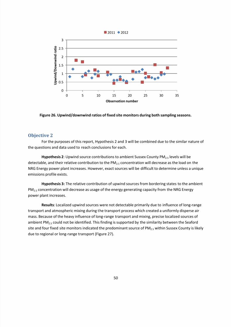
To support the finding that the NRG Energy power plant did not affect the Sussex County PM2.5

concentrations average daily wind directions identified the fixed site monitors located downwind andupwind of the power during each day of the study for both seasons (Figure 26). A ratio of

upwind/downwind mass concentrations less than unity indicates a source of PM2.5 between the two

monitors in question. During the first season the average upwind/downwind ratio of 1.7 ± SD 1.6

indicated no significant sources of PM2.5 between the two monitors. The same analysis carried out

during Season 2 resulted in an upwind/downwind ratio of 0.9 ± SD 0.2. At a level of α=0.01, the

upwind/downwind ratios between seasons are not statistically different, resulting in the conclusion that

the operating conditions of the power plant during the second season do not contribute to the local

PM2.5 in an appreciable amount in comparison to regional and long-range transport.



50

Figure 26. Upwind/downwind ratios of fixed site monitors during both sampling seasons.

Objective 2

For the purposes of this report, Hypothesis 2 and 3 will be combined due to the similar nature of

the questions and data used to reach conclusions for each.

Hypothesis 2: Upwind source contributions to ambient Sussex County PM2.5 levels will be

detectable, and their relative contribution to the PM2.5 concentration will decrease as the load on the

NRG Energy power plant increases. However, exact sources will be difficult to determine unless a unique

emissions profile exists.

Hypothesis 3: The relative contribution of upwind sources from bordering states to the ambient

PM2.5 concentration will decrease as usage of the energy generating capacity from the NRG Energy

power plant increases.

Results: Localized upwind sources were not detectable primarily due to influence of long-range

transport and atmospheric mixing during the transport process which created a uniformly disperse air

mass. Because of the heavy influence of long-range transport and mixing, precise localized sources of

ambient PM2.5 could not be identified. This finding is supported by the similarity between the Seaford

site and four fixed site monitors indicated the predominant source of PM2.5 within Sussex County is likelydue to regional or long-range transport (Figure 27).

0

0.5

1

1.5

2

2.5

3

0 5 10 15 20 25 30 35

U p w i n d / D o w n w i n

d r a t i o

Observation number

2011 2012



51

Figure 27. Comparison of Seaford and four fixed site monitors PM2.5 concentrations during 2011 (Red,NRG Energy power plant not operating) and 2012 (Blue, power plant operating) sampling seasons.

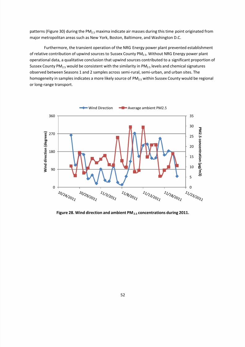
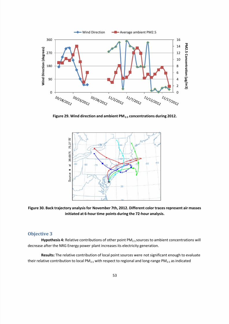
Figures 28 and 29 illustrate the PM2.5 concentration of the four fixed sites (averaged together)

and wind direction. Figure 29 illustrates an approximately 3 day delay between wind directed from

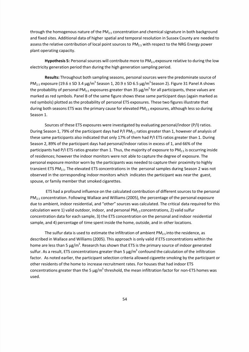
Northwest-North and maximum PM2.5 concentrations. 72-hr HYSPLIT back trajectory analysis of wind



52

patterns (Figure 30) during the PM2.5 maxima indicate air masses during this time point originated from

major metropolitan areas such as New York, Boston, Baltimore, and Washington D.C.

Furthermore, the transient operation of the NRG Energy power plant prevented establishment

of relative contribution of upwind sources to Sussex County PM2.5. Without NRG Energy power plant

operational data, a qualitative conclusion that upwind sources contributed to a significant proportion of Sussex County PM2.5 would be consistent with the similarity in PM2.5 levels and chemical signatures

observed between Seasons 1 and 2 samples across semi-rural, semi-urban, and urban sites. The

homogeneity in samples indicates a more likely source of PM2.5 within Sussex County would be regional

or long-range transport.

Figure 28. Wind direction and ambient PM2.5 concentrations during 2011.

0

5

10

15

20

25

30

35

0

90

180

270

360

P M2 . 5 c o n c e n t r a t i o n ( µ g / m 3 )

W i n d d i r e c t i o n ( d e g r e e s )

Wind Direction Average ambient PM2.5



53

Figure 29. Wind direction and ambient PM2.5 concentrations during 2012.

Figure 30. Back trajectory analysis for November 7th, 2012. Different color traces represent air masses

initiated at 6-hour time points during the 72-hour analysis.

Objective 3

Hypothesis 4: Relative contributions of other point PM2.5 sources to ambient concentrations will

decrease after the NRG Energy power plant increases its electricity generation.

Results: The relative contribution of local point sources were not significant enough to evaluate

their relative contribution to local PM2.5 with respect to regional and long-range PM2.5 as indicated

0

2

4

6

8

10

12

14

16

0

90

180

270

360 P M2 . 5

C o n c e n t r a t i o n ( µ g / m 3 )

W i n d D i r e c t i o n ( d e g r e e s )

Wind Direction Average ambient PM2.5



54

through the homogenous nature of the PM2.5 concentration and chemical signature in both background

and fixed sites. Additional data of higher spatial and temporal resolution in Sussex County are needed to

assess the relative contribution of local point sources to PM2.5 with respect to the NRG Energy power

plant operating capacity.

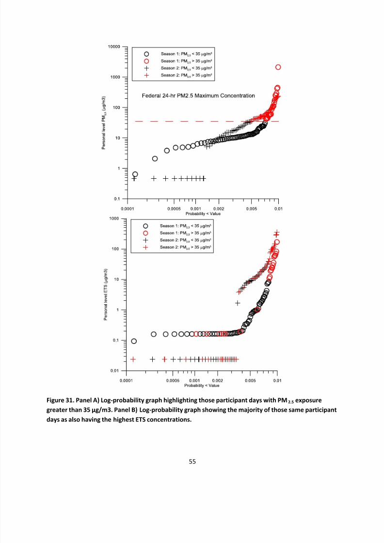
Hypothesis 5: Personal sources will contribute more to PM2.5 exposure relative to during the lowelectricity generation period than during the high generation sampling period.

Results: Throughout both sampling seasons, personal sources were the predominate source of

PM2.5 exposure (19.6 ± SD 3.4 µg/m3 Season 1, 20.9 ± SD 6.5 µg/m3 Season 2). Figure 31 Panel A shows

the probability of personal PM2.5 exposures greater than 35 µg/m3 for all participants, these values are

marked as red symbols. Panel B of the same figure shows these same participant days (again marked as

red symbols) plotted as the probability of personal ETS exposures. These two figures illustrate that

during both seasons ETS was the primary cause for elevated PM2.5 exposures, although less so during

Season 1.

Sources of these ETS exposures were investigated by evaluating personal/indoor (P/I) ratios.

During Season 1, 79% of the participant days had P/I PM2.5 ratios greater than 1, however of analysis of

these same participants also indicated that only 17% of them had P/I ETS ratios greater than 1. During

Season 2, 89% of the participant days had personal/indoor ratios in excess of 1, and 66% of the

participants had P/I ETS ratios greater than 1. Thus, the majority of exposure to PM2.5 is occurring inside

of residences; however the indoor monitors were not able to capture the degree of exposure. The

personal exposure monitor worn by the participants was needed to capture their proximity to highly

transient ETS PM2.5. The elevated ETS concentrations in the personal samples during Season 2 was not

observed in the corresponding indoor monitors which indicates the participant was near the guest,

spouse, or family member that smoked cigarettes.

ETS had a profound influence on the calculated contribution of different sources to the personal

PM2.5 concentration. Following Wallace and Williams (2005), the percentage of the personal exposure

due to ambient, indoor residential, and “other” sources was calculated. The critical data required for this

calculation were 1) valid outdoor, indoor, and personal PM2.5 concentrations, 2) valid sulfur

concentration data for each sample, 3) the ETS concentration on the personal and indoor residential

sample, and 4) percentage of time spent inside the home, outside, and in other locations.

The sulfur data is used to estimate the infiltration of ambient PM2.5 into the residence, as

described in Wallace and Williams (2005). This approach is only valid if ETS concentrations within the

home are less than 5 µg/m

3

. Research has shown that ETS is the primary source of indoor generatedsulfur. As a result, ETS concentrations greater than 5 µg/m3 confound the calculation of the infiltration

factor. As noted earlier, the participant selection criteria allowed cigarette smoking by the participant or

other residents of the home to increase recruitment rates. For houses that had indoor ETS

concentrations greater than the 5 µg/m3 threshold, the mean infiltration factor for non-ETS homes was

used.



55

Figure 31. Panel A) Log-probability graph highlighting those participant days with PM2.5 exposure

greater than 35 µg/m3. Panel B) Log-probability graph showing the majority of those same participant

days as also having the highest ETS concentrations.



56

Table 16 presents the apportionment of the participant’s PM2.5 exposure due to ambient, indoor

residential and “other” sources. The “other” sources category has three components. The main

component is the participant’s proximity to localized sources within the home since they may be

performing the activity or near the resident that is. Typical indoor sources with strong spatial gradients

include cigarette smoking, cooking, and cleaning (Rea et al., 2002). The indoor residential portion is the

PM2.5 concentration sampled by the indoor stationary PM2.5 sampler. This sampler is usually placed in a

common area of the house (e.g., family room), but not always. The ambient portion is PM2.5 that

infiltrates into the home via open windows, opening/closing doors, ventilation systems, and gaps around

windows, doors, and other exterior openings.

Table 16. Percentage of the personal PM2.5 exposure due to ambient, indoor residential, and other

sources. Data are presented by season, and stratified by residences without significant ETS and all

residences (ETS and non-ETS). Average and standard deviation for each source are presented.

Ambient and indoor percentages are calculated from the personal, indoor, and outdoor data. The

“Other” source consists of proximity to localized sources within the participant’s home,

transportation, and indoors at other locations; it is calculated by difference.

Source

Season 1

(No ETS)

Season 1

(All)

Season 2

(No ETS)

Season 2

(All)

Ambient 57% ± SD 30% 44% ± SD 30% 48% ± SD 53% 14% ± SD 15%

Indoor Residential 23% ± SD 33% 26% ± SD 34% 46% ± SD 65% 15% ± SD 17%

Other 22% 30% 8% 71%

# Observations 42 60 18 64

The impact of ETS on the apportionment of the three sources is clearly evident. The Season 1

and Season 2 apportionment for non-ETS residences are consistent with previous studies conducted in

the U.S. (Wallace and Williams, 2005; Rodes et al., 2010). When ETS is added, the percentage

contributed by ambient and indoor residential sources decreases and the “other” category increases.

This change is expected because of the strong source-proximity effect resulting from ETS. The impact of

ETS on the source contribution percentages is especially large in Season 2 since only 28% of the

comparisons came from non-ETS homes, as opposed to 70% from non-ETS homes in Season 1.

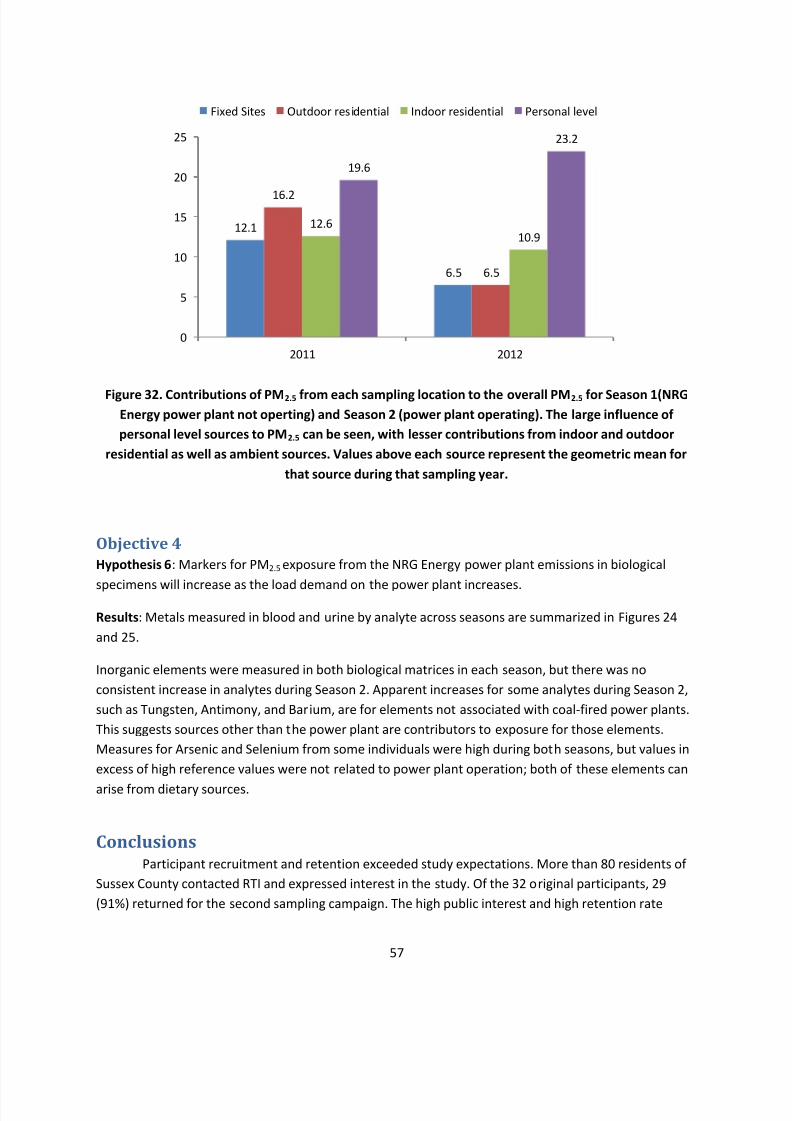
Furthermore, indoor and personal samples contained additional elements not found in outdoor

samples, such as Bromine, Copper, and Phosphorus. These factors coupled with the greater than 80% of

time spent indoors by the participants (as determined from questionnaire data) leads to the conclusion

that the greatest exposure to PM2.5 of the Sussex County population is occurring within indoorenvironments (Figure 32), while the most extreme events resulted from ETS, cooking, and cleaning.

Elevated exposure during these events is expected and has been previously documented (Rea et al.,

2002).



57

Figure 32. Contributions of PM2.5 from each sampling location to the overall PM2.5 for Season 1(NRGEnergy power plant not operting) and Season 2 (power plant operating). The large influence of

personal level sources to PM2.5 can be seen, with lesser contributions from indoor and outdoor

residential as well as ambient sources. Values above each source represent the geometric mean for

that source during that sampling year.

Objective 4

Hypothesis 6: Markers for PM2.5 exposure from the NRG Energy power plant emissions in biological

specimens will increase as the load demand on the power plant increases.

Results: Metals measured in blood and urine by analyte across seasons are summarized in Figures 24

and 25.

Inorganic elements were measured in both biological matrices in each season, but there was no

consistent increase in analytes during Season 2. Apparent increases for some analytes during Season 2,

such as Tungsten, Antimony, and Barium, are for elements not associated with coal-fired power plants.

This suggests sources other than the power plant are contributors to exposure for those elements.

Measures for Arsenic and Selenium from some individuals were high during both seasons, but values in

excess of high reference values were not related to power plant operation; both of these elements can

arise from dietary sources.

ConclusionsParticipant recruitment and retention exceeded study expectations. More than 80 residents of

Sussex County contacted RTI and expressed interest in the study. Of the 32 original participants, 29

(91%) returned for the second sampling campaign. The high public interest and high retention rate

12.1

6.5

16.2

6.5

12.610.9

19.6

23.2

0

5

10

15

20

25

2011 2012

Fixed Sites Outdoor residential Indoor residential Personal level



58

indicated Sussex County residents are interested in their health and quality of life. The community

interest and data quality achievements indicate statewide, longitudinal, multimedia exposure studies

are feasible.

Sampling conducted for PM2.5 during the fall of 2011 and 2012 indicated the geometric mean

ambient PM2.5 concentrations of the Millsboro area was 9.3 µg/m3

. The semi-rural location of Seafordhad an average PM2.5 concentration of 8.9 µg/m3, both below the Federal Standard of 15 µg/m3 and

were not statistically different at a test value of α=0.01. Sampling conducted outdoors and indoors of 35

distinct participants (32 each season) resulted in average PM2.5 concentrations of 11.3 µg/m3 and 11.8

µg/m3 respectively. The higher elevated indoor concentration is expected due to the strength and

proximity of PM2.5 sources found indoors (e.g. cooking, cleaning, candle burning, smoking, etc.). Personal

level sampling conducted during both seasons revealed geometric mean PM2.5 concentrations of 20.3

µg/m3 across both seasons. Similar to indoor PM2.5 measurements that were elevated with respect

outdoor and ambient measurement, higher personal level concentrations were presumably due to

personal proximity and strength of sources and is to be expected based on previous studies.

Analysis of the chemical and time-series analysis of the ambient PM2.5 of Sussex county reveals

the predominate source of PM2.5 within Sussex county to be regional and long-range transport of PM2.5

from upwind metropolitan locations such as Baltimore, New York City, and Boston. This can be observed

from the homogeneity of PM2.5 from a concentration as well as a compositional standpoint.

Additionally, though not part of the MIEBS, it is conceivable that due to the design of the NRG

Energy power plant stacks, the exhaust plume may lead to the majority of the PM2.5 to be deposited at

great distance from the stack, perhaps in the Atlantic. However, pollutants deposited by this mechanism

would be subject to significant dilution.

Despite the fact that control of much of the PM2.5 within Sussex County is beyond the control of Delaware officials, the majority of participants spent more than 80% of their day inside their own

homes. Thus RTI recommends performing a more detailed study of indoor PM2.5 sources as these

sources dominate the exposure of the Sussex County population to PM2.5. Results from this follow-up

study can be used to design an educational plan for the local population in an effort to reduce their

exposure and improve their long-term health.

The personal PM species measured do not have a strong and consistent contribution to the

analytes measured in the blood and urine from the study participants. The lack of a relationship may

mean that current exposures do not result in large biospecimen changes on the time scale of this study.

These data might also indicate the possibility of non-inhalation routes of exposure. Dietary and non-dietary ingestion of inorganic species should be considered for future investigation.

RecommendationsThe findings from this study suggest several recommendations for future research into the

environmental exposures that impact the health of Delaware residents. The recommendations are easily



59

separated into two groups: 1) additional analyses that can be performed using the collected biological,

PM2.5 and survey data and 2) future data collection and analysis efforts.

Recommendations for further analysis of the existing samples and dataset are summarized

below.

The PM2.5 emission from the NRG Energy power plant and the resulting concentration in the

ambient air within the study area should be modeled. This analysis will estimate the fraction of

the ambient PM2.5 contributed by the power plant. RTI wanted to perform this modeling for this

report. However, the fact the power plant operated under a variable load during Fall 2012

prohibits performing any modeling until NRG Energy reports PM2.5 emission data to DNREC

(expected in late 2013). If this modeling is performed, this report should be updated to

incorporate the results and revised conclusions.

Detailed statistical analysis of the PM2.5 and biospecimen data against the collected metadata is

recommended. The objectives of this report did not include a detailed analysis of the survey,

geospatial, or meteorological data in relation to the PM2.5 and biospecimen results. A

multivariate cluster analysis, such as principal component analysis, will identify variables or

classes of variables that predict the PM2.5 and biospecimen results. The findings from this

analysis would provide valuable information into the design of a larger, statewide multimedia

exposure study.

The additional analysis of PM2.5 and biospecimen samples will provide additional details to

clarify some of the findings or provide additional data for the multivariate analysis discussed

previously. The detailed recommendations listed below can be performed individually, as a

subset, or in total.

o The total arsenic mass in the urine should be speciated into organic and inorganic

fractions. CDC has a standard method for this analysis. This data will provide insight into

the toxicity and sources of the arsenic exposure noted in the report.

o The personal PM2.5 filters should be analyzed by inductively coupled plasma – mass

spectrometry (ICP-MS) to increase the number of elements per filter that are detected.

This data would be useful for the multivariate cluster analysis.

o Measure the urinary cotinine (biomarker of ETS exposure) to confirm ETS is a major

source of PM2.5 exposure in this study. The data from this inexpensive analysis would

provide further confirmation that the study participants were exposed to high levels of

tobacco smoke.

Multiple future studies are recommended to provide the information necessary to understand

the PM2.5 exposures of Sussex County residents and all Delaware residents.

There is a need to confirm long-range transport of PM2.5 from upwind urban areas is the primary

contributor to ambient PM2.5 concentrations in Delaware. A combination of ambient PM2.5



60

concentration measurements and Hysplit modeling will provide the information. RTI

recommends that daily PM2.5 samples be collected at an urban, suburban, and rural location for

at least four weeks in each season (Winter, Spring, Summer, Fall). The three sites can be existing

DNREC monitoring locations. Hysplit back-trajectory analysis, similar to the one conducted for

this study, will identify the origin of the ambient air up to 72 hours previously. A time series

correlation analysis will determine if the highest PM2.5 concentrations at the three monitoring

locations are correlated to air that originated over the metropolitan areas surrounding

Delaware.

A source apportionment study conducted at the DNREC Seaford site and one additional site near

the NRG Energy power plant would confirm the impact of long-range transport, regional

sources, and local sources (including the power plant) on PM2.5 concentrations and the Sussex

County residents’ exposure. This study would require detailed PM2.5 speciation data, including

metals (as measured for this study), nitrate, sulfate, and organic carbon fractions. Nitrogen

dioxide and sulfur dioxide gas concentration data would also be required.

Establish multimedia (air, dietary, and non-dietary ingestion) carcinogen exposure and

biospecimen distributions on a statewide level. This study would assess the broader, temporal

contribution of multiple sources to the total body burden of environmental contaminants and

account for individual behavior patterns. Exposure distributions would be captured by enrolling

participants in urban, suburban, and rural areas of Delaware and would help to establish the

baseline to monitor future exposures. This study would combine the Design I and Design II study

designs developed in 2008 (RTI, 2008).

As an initial step towards establishing a baseline, a study similar to that performed around

Millsboro could be conducted in the Wilmington area. This would provide for a comparison of

the rural Sussex County to an urban area with regard to the same pollutants. An expansion of

the methods to provide more data about the exposures (additional chemical measures in both

environmental and biological specimens) will begin to define those measures of greatest use in

the broader study.



61

ReferencesAndreae, M.O. and A. Gelencsér. 2006. “Black Carbon or brown carbon? The nature of light-absorbing

carbonaceous aerosol.” Atmospheric Chemistry and Physics 6:3131-3148.

Brown, K.W., Sarnat, J.A., and P. Koutrakis. 2012. “Concentrations of PM2.5 mass and components inresidential and non-residential indoor microenvironments: The Sources and Composition of

Particulates Exposures Study.” Journal of Exposure Science and Environmental Epidemiology

22:161-172.

Böhlandt, A., R. Schierl, J. Diemer, C. Koch, G. Bolte, M. Kiranoglu, H. Fromme, and D. Nowak. 2012.

“High concentrations of cadmium, cerium, and lanthanum in indoor air due to environmental

tobacco smoke.” Science of the Total Environment 414:738-741

Caldwell, K., R.L. Jones, C.P. Verdon, J.M. Jarrett, S.P. Caudill, and J.D. Osterloh. 2009. “Levels of urinary

total and speciated arsenic in the US population: National Health and Nutrition Examination

Survey 2003-2004.” Journal of Exposure Science and Environmental Epidemiology 19: 59-68.

CARB (California Air Resources Board). September 1998. Loss of Particle Nitrate from Teflon Sampling

Filters: Effects on Measured Gravimetric Mass. Sacramento, CA: California Air Resources Board,

Research Divison.

Cheung, K., N. Daher, W. Kam, M.W. Shafer, Z. Ning, J.J. Schauer, and C. Sioutas. 2011. “Spatial and

Temporal Variation of Chemical Composition and Mass Closure of Ambient Coarse Particulate

Matter (PM10 –2.5) in the Los Angeles Area.” Atmospheric Environment 45(16):2651-2662.

DNREC-OTS (Delaware Department of Natural Resources and Environment Control- Office of the

Secretary) June, 2008 Study Designs for Pilot Testing and a Multimedia, Total Exposure Study in

Delaware. Dover, DE: Delaware Department of Natural Resources and Environment Control-

Office of the Secretary.

DNREC (Delaware Department of Natural Resources and Environmental Control). September 2006.

Enhanced Delaware Air Toxics Assessment Study —E-DATAS Project Report . Dover, DE: Delaware

Department of Natural Resources and Environmental Control, Division of Air and Waste

Management.

Dockery, D.W. 2001. “Epidemiologic Evidence of Cardiovascular Effects of Particulate Air Pollution.”

Environmental Health Perspectives 109(Suppl 4):483-486.

Dzubay, T.G., R.K. Stevens, G.E. Gordon, I. Olmez, A.E. Sheffield, and W.J. Courtney. 1988. “A composite

receptor method applied to Philadelphia aerosol.” Environmental Science and Technology 22:46-

52.



62

Environment Canada-Health Canada. 2000. Priority Substances List Assessment Report: Respirable

Particulate Matter Less or Equal to Than 10 Micrometers Environment Canada. Gatineau,

Quebec: Environment Canada-Health Canada.

Goldberg, M.S., R.T. Burnett, J.C. Bailar, J. Brook, Y. Bonvalot, R. Tamblyn, R. Singh, and M.F. Valois.

2001. “The Association between Daily Mortality and Ambient Air Particle Pollution in Montreal,Quebec 1. Nonaccidental Mortality.” Environmental Research 86:12-25.

Greene, R. and E. Crecelius. 2006, “Total and inorganic arsenic in mid-atlantic marine fish and shellfish

and implications for fish advisories. Integrated Environmental Assessment and Management 2:

344-354.

Greene, R. 2010. Arsenic in the Delaware Inland Bays. November 5, 2010. Delaware Department of

Natural Resources and Environmental Control, Dover, DE.

Hoek, G., B. Brunekreef, P. Fischer, and J. Van Wijnen. 2001. “The Association between Air Pollution and

Heart Failure, Arrhythmia, Embolism, Thrombosis and Other Cardiovascular Causes of Death in aTime Series Study.” Epidemiology 12:355-357.

Ito, K., R. Mathes, Z. Ross, A. Nádas, G. Thurston, and T. Matte. 2011. “Fine Particulate Matter

Constituents Associated with Cardiovascular Hospitalizations and Mortality in New York City.”

Environmental Health Perspectives 119:467-473.

Johnson, D.L. 2008. “A first generation ingress, redistribution, and transport model of soil track-in:

DIRT.” Environmental Geochemistry and Health, 30:589-596, 2008.

Laden, F., L.M. Neas, D.W. Dockery, and J. Schwartz. 2000. “Association of fine Particulate Matter from

Different Sources with Daily Mortality in Six U.S. Cities.” Environmental Health Perspectives 108:941-947.

Lai, H.K., M. Kendall, H. Ferrier, I. Lindup, S. Alm, O. Hannien, M. Jantunen, P. Mathys, R. Colvile, M.R.

Ashmore, P. Cullinan, and M.J. Nieuwenhuijsen. 2004. “Personal exposures and

microenvironment concentrations of PM2.5, VOC, NO2, and CO in Oxford, UK.” Atmospheric

Environment 38:6399-6410.

Landis, M.S., G.A. Norris, R.W. Williams, and J.P. Weinstein. 2001. “Personal exposure to PM2.5 mass

and trace elements in Baltimore, MD, USA.” Atmospheric Environment 35:6511-6524.

Lawless, P.A., and Rodes, C.E. 1999. “Maximizing data quality in the gravimetric analysis of personalexposure sample filters”. Journal of the Air and Waste Management Association, 49:1039-1049.

Lawless, P.A., C.E. Rodes, and D.S. Ensor. 2004. Multiwavelength absorbance of filter deposits for

determination of environmental tobacco smoke and black carbon. Atmospheric Environment

38:3373 –3383.



63

Ondov, J.M., T.J. Buckley, P.K. Hopke, D. Ogulei, M.B. Parlange, W.F. Rogge, K.S. Squibb, M.V. Johnston,

A.S. Wexler. 2006. “Baltimore Supersite: Highly time- and size-resolved concentrations of urban

PM2.5 and its constituents for resolution of sources and immune responses.” Atmospheric

Environment 40:S224-S237.

Rea, A.W., C. Crogham, J. Thornburg, B. Rodes, and R. Williams. 2002. “PM concentrations associatedwith personal activities based on real-time personal nephelometry data from the NERL RTP PM

panel study.” Epidemiology 13:S82-S83.

Rodes, C.E., P.A. Lawless, J. Thornburg, R.W. Williams, and C. Croghan. 2010. DEARS “Particulate Matter

Relationships: Enhanced Personal, Indoor, Outdoor, and Central Site Exposure Data for a

General Population Cohort.” Atmospheric Environment 44:1386-1399.

RTI International. Study Designs for Pilot Testing and a Multimedia, Total Exposure Study in Delaware.

Final Report. PO 40-01010000777, June 20, 2008.

Suzuki, G., A. Kida, S. Sakai, and H. Takigami. 2009. “Existence state of bromine as an indicator of thesource of brominated flame retardants in indoor dust”. Environmental Science and Technology

43:1437-1442.

Thornburg, J., C.E. Rodes, P.A. Lawless, and R.W. Williams. 2009. “Sources and Causes of Coarse

Particulate Matter Spatial Variability in Detroit, MI.” Atmospheric Environment 43:4251-4258.

U.S. EPA (Environmental Protection Agency). 2004. Air Quality Criteria for Particulate Matter . U.S.

Environmental Protection Agency, Office of Research and Development, National Center for

Environmental Assessment, Washington, DC. August. Available at

http://cfpub2.epa.gov/ncea/cfm/recordisplay.cfm?deid=87903#Download.

Wallace, L. and R. Williams. 2005. “Use of personal-indoor-outdoor sulfur concentrations to estimate the

infiltration factor, outdoor exposure factor, penetration coefficient, and deposition rate for

individual homes.” Environmental Science and Technology 39:399-414.

Williams, R. J. Suggs, C. Rodes, P. Lawless, R. Zweidinger, R. Kwok, J. Creason, and L. Sheldon. 2000.

Comparison of PM2.5 and PM10 monitors.” Journal of Exposure Analysis and Environmental

Epidemiology 10:497-505.

Williams, R. J. Suggs, A. Rea, K. Leovic, A. Vette, C. Croghan, L. Sheldon, C. Rodes, J. Thornburg, A. Ejire,

M. Herbst, W. Sanders. 2003. The Research Triangle Park particulate matter panel study: PM

mass concentration relationships.” Atmospheric Environment 37:5349-5363.

Williams, R., Rappold, A.G., Case, M., Schmitt, M., Stone, S., Jones, P., Thornburg, J., and R.B. Devlin.

2012. “Multi-pollutant Exposures in an Asthmatic Cohort.” Atmospheric Environment 61:244-

252.

Zanobetti, A., J. Schwartz, and D.W. Dockery. 2000. “Airborne Particles Are a Risk Factor for Hospital

Admissions for Heart and Lung Disease.” Environmental Health Perspectives 108:1071-1077.

http://cfpub2.epa.gov/ncea/cfm/recordisplay.cfm?deid=87903%23Download.

http://cfpub2.epa.gov/ncea/cfm/recordisplay.cfm?deid=87903%23Download.



64

This page intentionally left blank



I

Appendices

Appendix A: Questionnaire Data

Table 17. Summarized participant questionnaire results Season 1.

race

transportation to

work

males femalesaverage

ageaverage weight

(lbs.)

average

height(inches) white

car, truck,or van

bus ortrolley

average

transit time(minutes)

average number

of years lived inSussex County

11 21 63.2 173.2 64.6 32 8 1 26 18.7

numbers reporting knowingly been exposed to any of the following

average

hours

away from

home

average

hours

outside

asbestos chemicals coal/dustcoal

tar/asphalt

diesel

engine

exhaust

dyes formaldehyde gasoline exhaust

4.2 2.3 4 6 2 0 1 9 4 0

numbers reporting knowingly been exposed to any

of the following, continued

pesticides textilefibers

wooddust

x-rays /radioactive

material

6 1 3 17



II

Table 18. Summarized participant questionnaire results Season 2.

race

transportation to

work

males females

average

age

average weight

(lbs.)

average

height

(inches) white

car, truck,

or van

bus or

trolley

average

transit time

(minutes)

average number

of years lived in

Sussex County

11 21 63.4 181.7 66.9 32 7 0 27.1 19.8

numbers reporting knowingly been exposed to any of the following

average

hours

away from

home

average

hours

outside

asbestos chemicals coal/dustcoal

tar/asphalt

diesel

engine

exhaust

dyes formaldehyde gasoline exhaust

3.6 2.4 6 6 3 0 4 3 4 3

numbers reporting knowingly been exposed to any

of the following, continued

pesticides

textile

fibers

wood

dust

x-rays /

radioactivematerial

6 3 2 10



III

Table 19. Summarized residential questionnaire results Season 1.

type of home

mobile

home

one-family

detached

one family

attached

building with 2 or more

apartments

boat, RV,

van, etc other

9 19 1 0 0 2

location and use of garage

none,

detached,

or

separate

carport attached underneath parking one car

parking

two cars

parking

more than 2

cars

storage

only N/A

19 12 0 12 3 0 4 10

Type of heating

forced air

gas forced air oil

forced air

electric forced water, radiator

heat

pump

wood

burning

stove

fireplace,

gas

fireplace,

wood

12 2 6 0 5 3 1 1

Type of heating, continued

gas space

heater

kerosene

space heater

electric

space heater open stove/oven other

1 0 4 0 5

average

number

of years

resident

of this

building

average age

of building

(years)

average # of

people average # of children

how many

central AC

units (per

residence)

how many

window AC

units

storm

windows

present

kitchen

exhaust

fan (yes)

12.9 23.1 2 0 1 1 20 27



IV

Table 20. Summarized residential questionnaire results Season 2.

type of home

mobile

home

one-family

detached

one family

attached

building with 2 or more

apartments

boat, RV,

van, etc other

10 21 1 0 0 2

location and use of garage

none,

detached,

or

separate

carport attached underneath parking one car

parking

two cars

parking

more than 2

cars

storage

only N/A

21 13 0 13 3 0 5 13

Type of heating

forced air

gas forced air oil

forced air

electric forced water, radiator

heat

pump

wood

burning

stove

fireplace,

gas

fireplace,

wood

14 2 6 0 6 4 1 1

Type of heating, continued

gas space

heater

kerosene

space heater

electric

space heater open stove/oven other

1 0 4 0 5

average

number

of years

resident

of this

building

average age

of building

(years)

average # of

people average # of children

how many

central AC

units (per

residence)

how many

window AC

units

storm

windows

present

kitchen

exhaust

fan (yes)

12.9 22.3 2 0 1 1 16 21





VI

Appendix B: Reference Ranges for Analytes in Blood or Serum

Analyte Monitored Fluid

Reference Range,

95th

Percentile

NHANES 2013,

ng/mL [i] Reference Ranges

[ii]

High Value (µg/L)

[iii, iv]

Cadmium Blood 1.55 <5 μg/L >5 μg/L

Lead Blood 3.57 μg/dL <30 μg/dL >40 μg/dL

Mercury Blood 5.75 <10 μg/L >200 μg/L

1,2-Dichloroethane Serum Not Available Not defined Not defined

Benzene Serum 0.34 Not defined Not defined

Carbon tetrachloride Serum<LOD Not defined Not defined

Chloroform Serum Not Available Not defined Not defined

Ethylbenzene Serum0.15 Not defined Not defined

m- & p-Xylene Serum0.43 Not defined Not defined

o-Xylene Serum0.11 Not defined Not defined

Styrene Serum 0.15 Not defined Not defined

Tetrachloroethylene Serum0.13 Not defined Not defined

Toluene Serum0.90 Not defined Not defined

[i] Fourth National Report on Human Exposure to Environmental Chemicals, updated Tables for Adults over 20 years, March 2013,Centers for Disease Control and Prevention National Center for Environmental Health (NCEH), Environmental Health Laboratory.[ii] Tietz Textbook of Clinical Chemistry, edited by C.A. Burtis and E.R. Ashwood, 1999

[iii] Carson, B.L., Ellis III H.V., and McCann, J.L., Toxicology and Biological Monitoring of Metals in Humans, Lewis Publishers, 1986.[iv} “High” levels are repeat upper boundary levels; samples with results greater than this range are reanalyzed for confirmation.

http://c/Documents%20and%20Settings/jraymer/Local%20Settings/Temporary%20Internet%20Files/Content.Outlook/BYTHZJP2/2012%20DPHL%20Biomonitoring%20Data%20Summary%20REPORTED.xlsx%23RANGE!A29

















VII

Appendix C: Reference Ranges for Analytes in Urine

Element/ IsotopeMonitored Fluid

Reference Range, 95th Percentile

NHANES 2013, ng/mL [i] High Value (μg/L, PPB) [ii]

Beryllium Urine <LOD 0.2

Cobalt Urine 1.35 2.83

Molybdenum Urine 144 293.5

Cadmium Urine 1.13 2.54

Antimony Urine 0.220 0.8

Cesium Urine 11.1 16.5

Barium Urine 6.80 17.1

Tungsten Urine0.370 1.38Platinum Urine 0.017 0.1

Thallium Urine 0.410 0.62

Lead Urine 1.71 7.8

Uranium Urine 0.36 0.277

Arsenic, total Urine 93.1 64.5

Selenium, total Urine 30.9[iii]

68

[i] Second National Report on Human Exposure to Environmental Chemical, hhtp://cdc.gov/exposurereport/2nd

/metal.htm, Centers

for Disease Control and Prevention, 2013.[ii] Values provided by DE DHSS (Call level). “High “values are repeat upper boundary levels; samples with results greater than this

are reanalyzed for confirmation

[iii] value provided by DE DHSS; referenced as NHANES 1999-2000









VIII

Appendix D: Data Quality Indicator Determination Methods

Quantitative data quality indicators (DQIs) targeted for each metric collected are presented in

Tables 3 and 4. DQIs include method detection limit (MDL), precision, accuracy, and completeness.

Qualitative DQIs include representativeness and comparability. Quality control sample results from the

outdoor, indoor, and fixed sites were combined to increase the statistical strength of the DQIs.

Collocated duplicate samples from all locations were combined to calculate the precision of the PEMs.

Field blanks and standard weight analyses were combined when calculating the MDL and MQL values for

the PEMs. This approach is reasonable given the same sampler (PEMs) was deployed at each location

and the filter underwent identical analysis (gravimetric, ETS/BrC, and BC).

Precision Precision is the agreement between the measurements collected by two identical devices or

measures under similar conditions. Collection of collocated duplicate samples provides information on

the variability in the sample collection, handling, storage, and analysis. Precision is reported as percent

relative standard deviation (% RSD) between replicate samples or sample analyses and is defined as

where SD is the standard deviation and Mean is the mean value of the measurements from each

replicate set.

Accuracy and Bias Accuracy is the measure of the closeness of a measured value to a known or true value and

includes both random error (precision) and systematic error (bias). Precision was discussed previously.

Bias is the distortion of the data in a consistent direction due to measurement or analytical error.

Measurement and analytical bias should be estimated using materials as independent as possible from

the measurement system.

Measurement accuracy is used to assess sample collection with the integrated and continuous

instrumentation. Measurement accuracy will be reported as a comparison between the measured value

and the known value of a standard. Accuracy is defined as

where Cstd and Csample are the values for the standard and the sample, respectively. Measurement

accuracy for instrumentation typically is determined by the validation of the instrument performance

during instrument development. For continuous monitors, accuracy also is determined during

instrument calibration certification.



IX

Analytical accuracy will be reported as recovery from spiked control samples during sample

analysis. The composition and concentration of the spiked sample will come from a standard reference

material (e.g., National Institute of Standards and Technology [NIST]). Recovery is defined as

where Cm, Cu, and Cs are the concentration of each target analyte measured in the spiked sample, in the

unspiked sample, and the spiking solution, respectively. This definition of analytical accuracy

incorporates matrix recovery into the assessment. A documented, consistent spiking protocol is

essential to obtain useful accuracy estimates.

Table 22. Target DQI's for each metric and analyte.

Metric Analysis MDL/MQL Precision Accuracy

% Complete

Collection Analysis

RTI MicroPEM Gravimetric 1.4/4.2 µg/m3

±10% ±15% 95% 99%

ETS 2.4/7.2 µg/m3

±10% ±15% 95% 99%

BC 0.4/1.2 µg/m3

±10% ±15% 95% 99%

XRF See Table 2-2

2 Lpm PEM Gravimetric 0.2/0.6 µg/m3

±10% ±10% 95% 99%

ETS/BrC 0.3/0.9 µg/m3

±10% ±10% 95% 99%

BC 0.1/0.3 µg/m3

±10% ±10% 95% 99%

XRF See Table 2-2

Questionnaires NA NA NA NA 99% NA

HOBO NA NA NA NA 99% NA

Completeness Completeness is a measure of valid data obtained from each metric. Completeness consists of

sample collection and analysis components. Completeness requirements for sample collection and

analysis aspects are presented because their relative importance varies between metrics. Completeness

is typically defined by RTI as follows for all chemical and physical measurements:



X

where V is the number of measurements judged valid, and N is the number of measurements planned.

The anticipated influence of completeness for each metric on the ability to answer the study hypotheses

should be considered when the statistical design for the study is being developed.

Other Quality Criteria Instrument Detection Limit (IDL)

The quantity of the target analyte that can be measured and distinguished from zero on a

continuous monitor provides direct output of the metric of interest. It is the lowest level readable on a

display or recorded that can be distinguished from background.

Method Detection Limit (MDL), Corrected for Optimal Sample Volume

The method detection limit (MDL) is defined as the minimum concentration of substance that

can be measured and reported with a known confidence that the analyte concentration is greater than

zero and is determined from analysis of a sample in a given matrix containing the analyte. For allapplicable metrics, the equation to determine the MDL for a given analyte is:

MDL = t(n-1, a=0.68)S

where, t(n-1, a = 0.68) represents the Students’ t-test t value appropriate for a 68% confidence level

(84% one-tailed) and a standard deviation estimate with n-1 degrees of freedom. S is equal to the

standard deviation of the replicate (usually seven samples) analyses. This value is obtained from

analyzing standard samples containing the target mass between the MDL and the lowest target analyte

mass expected to be observed (or blank filters for filter media). This value is then divided by the

theoretical sample volume. For example, the theoretical volume for a 24 h PM sample collected on aPEM sampler operating at 4 L per minute is 5,760 L or 5.76 cubic meters.

Method Quantitation Limit (MQL)

For other analyses, such as gravimetric, the MQL is three times the MDL [MQL = 3 x MDL] and

within the specified limits of precision and accuracy during routine analytical operating conditions.

Tables 4 and 5 contain the current values of MQL.



XI

Table 23. Target quantitative DQI's for XRF analysis.

Element MDL/MQL ng/filter Precision Accuracy

% Completeness

Collection Analysis

Sodium 70/210 20 10 95% 99%

Magnesium 70/210 20 10 95% 99%

Aluminum 500/1,500 20 10 95% 99%

Silicon 170/510 20 10 95% 99%

Phosphorous 120/360 20 10 95% 99%

Sulfur 70/210 20 10 95% 99%

Chlorine 50/150 20 10 95% 99%

Potassium 30/90 20 10 95% 99%

Calcium 40/120 20 10 95% 99%

Titanium 70/210 20 10 95% 99%

Vanadium 25/75 20 10 95% 99%

Chromium 10/30 20 10 95% 99%

Manganese 10/30 20 10 95% 99%

Iron 30/90 20 10 95% 99%

Cobalt 20/60 20 10 95% 99%

Nickel 15/45 20 10 95% 99%

Copper 15/45 20 10 95% 99%

Zinc 10/30 20 10 95% 99%

Arsenic 15/45 20 10 95% 99%

Selenium 8/24 20 10 95% 99%

Bromine 10/30 20 10 95% 99%

Rubidium 10/30 20 10 95% 99%

Strontium 10/30 20 10 95% 99%

Zirconium 80/240 20 10 95% 99%

Silver 50/150 20 10 95% 99%

Cadmium 60/180 20 10 95% 99%

Tin 80/240 20 10 95% 99%

Antimony 90/270 20 10 95% 99%



XII

Element MDL/MQL ng/filter Precision Accuracy

% Completeness

Collection Analysis

Cesium 133/400 20 10 95% 99%

Barium 170/510 20 10 95% 99%

Cerium 467/1,400 20 10 95% 99%

Mercury 23/70 20 10 95% 99%

Lead 24/72 20 10 95% 99%



XIII

Table 24. Actual DQIs from MIEBS Seasons 1 & 2.

Metric Analysis MDL/MQL Precision* Accuracy

% Complete

Collection Analysis

RTI MicroPEM Gravimetric:Season 1

Season 2

0.1/0.4 µg/m3

0.2/0.7 µg/m3

-

-

0.1%

0.1%

See Table 7

See Table 8

See Table 7

See Table 8

ETS:

Season 1

Season 2

0.04/0.1 µg/m3

0.01/0.03 µg/m3

-

-

-

-

See Table 7

See Table 8

See Table 7

See Table 8

BC

Season 1:

Season 2:

0.01/0.03 µg/m3

0.03/0.08 µg/m3

-

-

-

-

See Table 7

See Table 8

See Table 7

See Table 8

XRF See Table 7

PEM:2 LPM season 1

4 LPM season 2

Gravimetric:Season 1

Season 2:

0.3/0.9 µg/m3

0.02/0.08 µg/m3

10.1%

14.8%

-5.5%

-5.5%

See Table 7

See Table 8

See Table 7

See Table 8

ETS/BrC:

Season 1

Season 2

0.3/1.0. µg/m3

0.008/0.002 µg/m3

17.6%

10.0%

-

-

See Table 7

See Table 8

See Table 7

See Table 8

BC:

Season 1

Season 2

0.3/1.0. µg/m3

0.008/0.002 µg/m3

2.6%

6.0%

-

-

See Table 7

See Table 8

See Table 7

See Table 8

XRF See Table 7

Questionnaires Season 1Season 2

NA NA NA 91%100%

NA

HOBO Season 1

Season 2

NA NA NA 100%

100%

NA

[*]Precision values are averages of all filters collocated filters: n = 7 Season 1; n= 14 Season 2

Table 25. Actual DQIs for XRF Analysis of MIEBS Season 1 & 2 data.

MDL (ng/filter) MQL (ng/filter) Median Precision Accuracy

Season 1 Season 2 Season 1 Season 2 Season 1Season

2

Season

1

Season

2

Ag 211.9 223.5 635.7 670.4 0.0 0.0 - -

Al 119.1 95.2 357.3 285.7 0.0 0.0 - -

As 12.1 10.8 36.2 32.5 0.0 0.0 - -

Ba 59.4 67.2 178.3 201.5 0.0 0.0 - -

Br 12.5 11.4 37.5 34.3 0.0 0.0 - -



XIV

MDL (ng/filter) MQL (ng/filter) Median Precision Accuracy

Ca 22.7 18.8 68 56.3 0.0 22.5 - -

Cd 283.1 299.5 849.4 898.6 0.0 0.0 0.0 -2.0

Ce 30.2 50.1 90.6 150.2 0.0 0.0 - -

Cl 22.6 18.4 67.8 55.1 0.0 0.0 - -Co 6.4 5.8 19.2 17.3 0.0 0.0 - -

Cr 10.9 11.6 32.8 34.9 0.0 0.0 - -

Cs 60.7 70.7 182.2 212.0 0.0 0.0 - -

Cu 10.1 6.6 30.4 19.9 0.0 0.0 - -

Fe 10.7 9.5 32 28.5 19.6 10.5 0.6 0.8

In 367.4 383.8 1102.1 1151.3 0.0 0.0 - -

K 19.1 17.9 57.2 53.8 9.4 10.9 - -

Mg 56.7 44.5 170.2 133.4 0.0 0.0 - -

Mn 8.8 8.8 26.4 26.5 0.0 0.0 - -

Na 131.4 92.4 394.2 277.3 0.0 0.0 - -

Ni 5.9 5.0 17.8 15.0 0.0 0.0 - -

P 45.7 4.7 137.2 14.0 0.0 0.0 - -

Pb 25.0 19.3 75 58.0 0.0 0.0 -0.8 1.8

Rb 13.7 13.8 41.2 41.3 0.0 0.0 - -

S 29.6 23.6 88.8 70.7 5.3 7.2 - -

Sb 712.5 709 2137.6 2127.1 0.0 0.0 - -

Se 13.5 11.7 40.4 35.1 0.0 0.0 1.3 -0.3

Si 57.4 47.7 172.3 143.2 33.1 27.1 1.1 -0.2

Sn 497.3 552.2 1491.8 1656.7 0.0 0.0 - -

Sr 18.2 154.7 54.7 464.0 0.0 0.0 - -

Ti 22.7 28.8 68.2 86.3 0.0 0.0 0.2 1.5

V 15.2 18.7 45.7 56.0 0.0 0.0 - -

Zn 10.1 7.7 30.2 23.0 0.0 27.7 - -

Zr 139.3 197.5 418 592.5 0.0 0.0 - -



XV

Data validity was determined on three levels: 1) review of data collection sheets recorded by

field technicians during sampling, 2) physical inspection of filters, and 3) comparison of analysis results

against other filters collected. During each of these steps filters were given one of three levels of

validity:

Invalid (code = 0; noted handling issue or obvious filter damage which precludes analysis)

Suspect (code = 1; no noted issues, but reported value is more or less than twice the standard

deviation of the mean)

Valid (code = 2; no noted issues and data value is within two standard deviations of the mean)

During the first level of data validation, any filters that were noted as incorrectly handled were marked

as invalid due to possible contamination. The second level of data review involved visual inspection of

filters for any holes which might induce errors in analytical analysis. The final level of data validation

resulted from comparison of analytical data amongst all filters of similar sample collection parameters.

All data was entered into a comprehensive file in order to provide a unified space for data to be housed.Results from the validation procedures are displayed in Tables 7 and 8.



GlossaryParticulate Matter (PM): Any material, except pure water, that exists in the solid or liquid state in the

atmosphere, such as soot, dust, smoke, fumes, and aerosols. The size of particulate matter can vary

from coarse, wind-blown dust particles to fine particle combustion products.

Particulate Matter less than 2.5 micrometers (PM2.5): A major air pollutant consisting of tiny solid orliquid particles, generally soot and aerosols. The size of the particles (2.5 micrometers or smaller, about

0.0001 inches or less) allows them to easily enter the air sacs deep in the lungs where they may cause

adverse health effects, as noted in several recent studies. PM2.5 also causes visibility reduction.

Volatile Organic Compound (VOC): This term is generally used similarly to the term "reactive organic

compounds" but excludes ethane, which the federal government does not consider to be reactive. VOCs

are hydrocarbon compounds that exist in the ambient air and contribute to the formation of smog

and/or may themselves be toxic. VOCs often have an odor, and some examples include gasoline,

alcohol, and the solvents used in paints.

Minimum Detection Limit (MDL): The minimum concentration of a substance that can be measured and

reported with 99 percent confidence that the analyte concentration is greater than zero and is

determined from analysis of a sample in a given matrix containing the analyte.

Minimum Quantification Limit: The smallest detectable concentration of analyte greater than the

detection limit where the required* accuracy (precision & bias) is achieved for the intended purpose.

Date post:	14-Apr-2018
Category:	Documents
Upload:	zackseward
View:	221 times
Download:	0 times