"Expected Utility - Mean Absolute Semideviation" Model of Individual Decision Making under Risk Pavlo R. Blavatskyy Institute of Public Finance University of Innsbruck Universitaetsstrasse 15 A-6020 Innsbruck Austria Phone: +43 (0) 512 507 71 56 Fax: +43 (0) 512 507 29 70 E-mail: [email protected]Abstract. This paper presents a new theory of decision under risk. Individual preferences over lotteries are assumed to be complete, transitive, continuous and satisfy transformed independence axiom. Such preferences admit representation of the form U(L)-ρ·r (L), where U(L) denotes the expected utility of lottery L, ρ∈[-1,1] is a constant and r (L) is the mean absolute (utility) semideviation of lottery L. The model is interpreted as a linear trade-off between expected utility and utility dispersion. The model is compatible with all major behavioral regularities. In particular, it respects stochastic dominance, allows for the Allais paradox and rationalizes switching behavior in the Samuelson's example. Key Words: Decision Theory, Expected Utility, Risk, Utility Dispersion, Mean- Variance Approach JEL Classification Codes: D00, D03, D81
Transcript
"Expected Utility - Mean Absolute Semideviation"Model of Individual Decision Making under Risk
Pavlo R. Blavatskyy
Institute of Public FinanceUniversity of InnsbruckUniversitaetsstrasse 15
Abstract. This paper presents a new theory of decision under risk. Individual preferences over lotteries are assumed to be complete, transitive, continuous and satisfy transformed independence axiom. Such preferences admit representation of the form U(L)-ρ·r (L), where U(L) denotes the expected utility of lottery L, ρ∈[-1,1] is a constant and r (L) is the mean absolute (utility) semideviation of lottery L. The model is interpreted as a linear trade-off between expected utility and utility dispersion. The model is compatible with all major behavioral regularities. In particular, it respects stochastic dominance, allows for the Allais paradox and rationalizes switching behavior in the Samuelson's example.
The goal of this paper is to develop a new theory of individual decision making under risk that fulfills three basic requirements. First, a theory is developed in a general framework of von Neumann and Morgenstern (1944). In other words, possible outcomes (consequences) are arbitrary and not restricted only to monetary payoffs. Second, a theory is derived from basic assumptions (axioms) about individual preferences over risky alternatives and it has a normatively appealing interpretation (both in terms of economic intuition and aesthetically pleasing algebra). Third, a theory is descriptively adequate in a sense that it is consistent with all major behavioral regularities. In particular, it does not violate the first-order stochastic dominance and it can account for the Allais paradox (Allais, 1953).
A new theory can be summarized as follows. Let L: X → [0,1] denote a lottery, i.e., a probability distribution on an arbitrary set X of possible outcomes. An individual has a preference relation ≿ over lotteries. We assume that this preference relation is complete, transitive, continuous and satisfies the transformed independence axiom. The first three axioms are standard assumptions about individual preferences (cf. von Neumann and Morgenstern, 1944). The transformed independence axiom is a new preference condition that is not used in the existing literature.
If a preference relation ≿ satisfies four proposed axioms then there exist a utility function u:X→ℝ and a constant ρ ∈[-1,1] such that:(1) L ≿ L' if and only if U(L)-ρ·r (L) ≥ U(L' )-ρ·r (L' ),where(2) U(L)=∑x∈X L(x)u(x) is the expected utility of lottery L and(3) r (L)=0.5∑x∈X L(x)·|U(L)-u(x)| is the mean absolute semideviation of utility of L's outcomes from the expected utility of L. Model (1)-(3) is a parsimonious one-parameter generalization of expected utility theory. The latter emerges as a special case of representation
2
(1) when coefficient ρ is equal to zero.Model (1)-(3) has an intuitive economic interpretation. Quantity r (L)
captures utility dispersion of lottery L. In particular, r (L)=0 when L is a degenerate lottery that yields one outcome for certain (i.e., L bares no risk) or when an individual is indifferent between all outcomes in L that have a strictly positive probability of occurrence (i.e., L has de facto no risk exposure). For all other lotteries quantity r (L) is strictly positive. Quantity r (L) is related to risk measures commonly used in engineering and finance.
If quantity r (L) measures utility dispersion of lottery L then it is natural to think that a coefficient ρ ∈[-1,1] captures individual attitude towards risk. A positive value of ρ∈(0,1] denotes risk aversion. In this case, representation (1) is simply a linear trade-off between expected utility and risk. An individual prefers lotteries with a higher expected utility and a lower utility dispersion. A negative value of ρ∈[-1,0) denotes risk seeking (loving). In this case, there is no trade-off: an individual prefers lotteries with higher expected utility and higher utility dispersion. In a special case when ρ=0 an individual does not care about utility dispersion and acts as a neoclassical expected utility maximizer.
Model (1)-(3) is not only a simple and intuitively appealing theory but it also has a significant descriptive merit. The model is consistent with all major behavioral regularities. Moreover, it can account for most behavioral patterns only when its coefficient ρ is positive (cf. Table 1 below). This is in line with economic intuition behind the model. Most behavioral regularities can be driven by a simple fact that people do not only seek to maximize their expected utility but they are also exhibiting aversion to utility dispersion.
Behavioral regularities listed in Table 1 have seemingly little in common, except for the fact that they are all persistently documented over and over again in empirical studies. However, these diverse behavioral patterns fit together as pieces of one puzzle once we look at them through the lens of risk aversion. This is perhaps the most important contribution of this paper.
3
╔═══════════════════════╦═══════════╗║ Behavioral regularity ║Necessary condition ║╠═══════════════════════╬═══════════╣║Stochastic dominance is not violated ║ ρ ∈[-1,1] ║╠═══════════════════════╬═══════════╣║The common ratio effect ║ ρ ∈(0,1) ║╠═══════════════════════╬═══════════╣║The common consequence effect (Allais paradox) ║ ρ ∈(0,1] ║╠═══════════════════════╬═══════════╣║Vertical fanning-in in the probability triangle ║ ρ ∈(0,1] ║╠═══════════════════════╬═══════════╣║The betweenness axiom is violated ║ ρ ≠0 ║╠═══════════════════════╬═══════════╣║The fourfold pattern of risk attitudes ║ρ∈(0,1] & u(.) is convex ║║ ║ρ∈[-1,0) & u(.) is concave║╠═══════════════════════╬═══════════╣║Switching behavior in the Samuelson's example ║ ρ ∈(0,1] ║╚═══════════════════════╩═══════════╝
Table 1 Necessary conditions in model (1)-(3) for various behavioral regularities
The model presented in this paper resembles the mean-variance approach (Markowitz, 1952). However, there is a fundamental difference between the two. The mean-variance approach lacks axiomatic foundation. It uses an ad hoc risk measure (variance or standard deviation) that violates stochastic dominance (e.g., Borch, 1969). In contrast, the model presented in this paper is derived from four basic assumptions about individual preferences. This imposes a good deal of rational structure on the derived representation. In particular, our model always respects (first-order) stochastic dominance.
There is also another important difference. The mean-variance approach does not use the concept of utility, i.e., the risk of a lottery is an objective characteristic. In contrast, representation (1) has a subjective utility function. In this model, people care about subjective utility dispersion not an objective risk, i.e. two individuals may disagree on the riskiness of the same lottery.
In terms of descriptive merit, there are only few other theories that can accommodate all behavioral regularities listed in Table 1. One of them is the perceived relative argument model (PRAM) recently proposed by Loomes (2008). PRAM does not have axiomatic foundation and allows for intransitive preferences over risky alternatives. In contrast, the model presented in this
4
paper is derived from four primitive assumptions about individual preferences. One of these assumptions is transitivity of preferences.
Another prominent descriptive model is rank-dependent utility theory (RDU) proposed by Quiggin (1981). RDU has axiomatic foundation (e.g. Abdellaoui, 2002) but the model faces difficulties when it comes to explaining the Samuelson's example. That is why Tversky and Kahneman (1992) extended RDU model by introducing the possibility of loss aversion. The extended model is known as cumulative prospect theory (CPT). CPT rationalizes all behavioral patterns listed in Table 1 as a consequence of either non-linear probability weighting or loss aversion. In contrast, the model presented in this paper is more parsimonious—behavioral regularities listed in Table 1 are explained by individual aversion to utility dispersion. Additional behavioral assumptions, such as loss aversion, are not necessary within this model.
The remainder of the paper is structured as follows. The next section presents a formal framework, four proposed axioms and the representation theorem. Section 2 goes over behavioral implications of this model. Section 3 concludes with a general discussion.
5
1. TheoryLet X be a finite non-empty set of possible outcomes (consequences).
Set X is an abstract set, not necessarily a subset of the Euclidian space ℝn. A lottery L: X → [0,1] is a probability distribution on X, i.e., L(x)∈[0,1] for all x∈Xand ∑x∈X L(x)=1. For simplicity, a degenerate lottery that yields one outcome x∈X with probability one is denoted by x. The set of all lotteries is denoted by ℒ. Notation LαL' denotes a compound lottery that yields lottery L with probability α∈[0,1] and lottery L' with probability 1-α.
A decision maker has a preference relation ≿ on ℒ. As usual, the sign ≻ denotes the asymmetric component of ≿ and the sign ~ denotes the symmetric component of ≿. We assume that the preference relation ≿ satisfies the following three axioms.Axiom 1 (Completeness) For any L,L' ∈ℒ either L ≿ L' or L' ≿ L (or both).Axiom 2 (Transitivity) For any L, L', L" ∈ℒ if L ≿ L' and L' ≿ L" then L ≿ L".Axiom 3 (Continuity) For any L, L', L" ∈ℒ the sets {α∈[0,1] : LαL' ≿L" } and {α∈[0,1] : L" ≿LαL' } are closed.
Before presenting the fourth and final assumption about individual preferences, it is necessary to introduce a new concept of a transformed lottery. Consider a binary lottery L that yields either an outcome x∈X or an outcome y∈X, x≿y. This lottery can be transformed into a new lottery Lρ as follows: Lρ(x)=L(x)·[1-ρ·L(y)] and Lρ(y)=L(y)·[1+ρ·L(x)]. Note that if ρ ∈[-1,1] then the transformed lottery Lρ is a well-defined probability distribution on X (i.e., Lρ∈ℒ) for any binary lottery L∈ℒ. If lottery L is a degenerate lottery that yields one outcome for certain then the transformed lottery Lρ is the same degenerate lottery (i.e., Lρ=L). In a special case when ρ=0, the transformed lottery Lρ is identical to the original lottery L for any binary lottery L∈ℒ.
When ρ∈(0,1], the transformation works as follows. On the one hand, the probability of a desirable outcome x is decreased. In percentage terms, this decrease is proportionate to the probability of an undesirable outcome y in the
6
original lottery L. On the other hand, the probability of an undesirable outcome y is increased. In percentage terms, this increase is proportionate to the probability of a desirable outcome x in the original lottery L. Intuitively, when ρ∈(0,1], we can imagine that the transformed lottery Lρ is the perception of a risky lottery L by a risk averse individual who downplays (exaggerates) the likelihood of a desirable (undesirable) outcome.
When ρ∈[-1,0), the transformation works in the opposite direction. Probability of a desirable outcome increases and probability of an undesirable outcome decreases. Intuitively, in this case, we can imagine that the transformed lottery is the perception of lottery L by a risk loving individual.
Let us now consider a more general case when lottery L yields more than two outcomes. Suppose that an outcome z∈X and any outcome that is at least as good as z are desirable outcomes (all remaining outcomes are undesirable). Then any lottery L∈ℒ can be transformed into a new lottery Lρ as follows:
L(x)·[1-ρ·∑y∈X, z≻y L(y)], for any x∈X such that x ≿z(4) Lρ (x) =
L(x)·[1+ρ·∑y∈X, y≿z L(y)], for any x∈X such that z ≻x.
If ρ ∈[-1,1] then the transformed lottery Lρ is a well-defined probability distribution on X (i.e., Lρ∈ℒ) for any lottery L∈ℒ. Note that the transformed lottery Lρ is identical to the original lottery L only in two cases: when L is a degenerate lottery that yields one outcome for certain and when ρ=0. When ρ∈(0,1] the transformation works as follows. The probability of any desirable outcome is decreased. In percentage terms, this decrease is proportionate to the cumulative probability of all undesirable outcomes in the original lottery L. The probability of any undesirable outcome is increased. In percentage terms, this increase is proportionate to the cumulative probability of all desirable outcomes in the original lottery L. When ρ∈[-1,0) the probability of any desirable outcome is increased and the probability of any undesirable outcome is decreased during the transformation.
Table 2 Transformed lottery Lρ (d ≻ c ≻b ≻a , only a is undesirable)
Table 2 presents an example of transformation (4). The set of outcomes is {a, b, c, d } such that d ≻ c ≻b ≻a. Suppose that only outcome a is undesirable and all other outcomes are desirable. The original lottery is shown in the line that corresponds to ρ=0. Other lines in Table 2 present the transformed lottery Lρ for different values of ρ. For example, the probability of the worst outcome a is 0.2 in the original lottery. This probability is transformed into 0.36 (0.04) when ρ=1 (ρ=-1). This simple example illustrates that an individual with a positive (negative) coefficient ρ can significantly exaggerate (downplay) the chance of an undesirable outcome.
Now it remains only to define which outcomes are desirable and which are not. Clearly, the desirability of an outcome depends on a lottery. Consider a lottery that yields 100 Euros with probability 90%, 10 Euros with probability 5% and nothing with probability 5%. In the context of this lottery, a payoff of 10 Euros is likely to be an undesirable outcome for the majority of people. Now consider another lottery that yields 100 Euros with probability 5%, 10 Euros with probability 5% and nothing with probability 90%. In this context, a payoff of 10 Euros is likely to be a desirable outcome for the majority of people.
8
A natural candidate for capturing such lottery-dependent desirability of outcomes is elation/disappointment decomposition of lottery outcomes (Gul, 1991, p. 671). Gul (1991) divides the outcomes of lottery L into two groups: those that are preferred to the certainty equivalent of L (elation outcomes) and those that are not (disappointment outcomes). In our framework, the set of outcomes is not restricted to be a subset of ℝn, i.e. lotteries generally do not have certainty equivalents. Thus, elation/disappointment decomposition is not directly feasible but we can exploit the same idea in a roundabout manner.
Since the set of lottery outcomes X is finite and the preference relation ≿ on X is complete and transitive (Axioms 1 and 2), there must be the most preferred outcome x ̄∈X (i.e., x ̄ ≿x for any x∈X ) and the least preferred outcome x ̱∈X (i.e., x ≿x ̱ for any x∈X ). Furthermore, since the preference relation ≿ is continuous (Axiom 3), for any outcome x∈X, there is a number αx∈[0,1] such that x ~ x ̄αxx ̱. Finally, this number αx is unique if x ̄αx ̱ ≻ x ̄βx ̱ for any α>β. The latter property follows from Axiom 4 introduced below and there is no need to assume it explicitly.
To sum up, given our assumptions about preferences, for any outcome x∈X we can find a unique number αx∈[0,1] such that x ~ x ̄αxx.̱ In principle, we can use this number αx as a measure of "goodness" of outcome x as it is done in von Neumann and Morgenstern (1944). However, such approach warrants some caution. Suppose that an individual is indifferent between a degenerate lottery that yields x for certain and a binary lottery that yields x ̄ with probability αx and x ̱otherwise. The first lottery is a degenerate lottery that bares no risk. In contrast, the second lottery is a risky distribution. Hence, number αx does not only capture the "goodness" of outcome x but it also has some risk premium built into it. In other words, in general, number αx overestimates the "goodness" of outcome x. To correct for this bias, we need to scale αx down. We scale αx down using the same transformation, as already described above (for binary lotteries): αx,ρ =αx·[1-ρ·(1-αx)].
9
We treat number αx,ρ as a measure of "goodness" of outcome x∈X. In a similar vein, number ∑y∈X L(y)·αy,ρ captures the "goodness" of lottery L∈ℒ. It is natural to assume that an outcome x ∈X in lottery L∈ℒ is desirable when αx,ρ ≥ ∑y∈X L(y)·αy,ρ and it is undesirable when αx,ρ < ∑y∈X L(y)·αy,ρ . This completes our definition of a transformed lottery. For convenience, this notion is summarized in Definition 1 below.Definition 1 A transformed lottery Lρ of a lottery L∈ℒ is defined as
L(x)·[1-ρ·∑y∈X, z≻y L(y)], for any x∈X such that x ≿z Lρ (x) =
L(x)·[1+ρ·∑y∈X, y≿z L(y)], for any x∈X such that z ≻x,
where ρ ∈[-1,1] is a constant, z ∈X denotes the least preferred outcome such that αz·[1-ρ·(1-αz)] ≥ ∑y∈X L(y)·αy·[1-ρ·(1-αy)] and αy∈[0,1] denotes a number such that y ~ x ̄αyx ̱ for any outcome y ∈X.
Given the above definition, we can impose the fourth axiom on the preference relation ≿.Axiom 4 (Transformed Independence Axiom) There exist ρ ∈[-1,1] such that for any L, L', L" ∈ℒ and any α∈[0,1] we have L ≿ L' if and only if S ≿ S' where S, S' ∈ℒ are two lotteries such that Sρ =LραL" and S'ρ =L'ραL".
In a special case when ρ=0, Axiom 4 becomes the independence axiom of expected utility theory (cf. von Neumann and Morgenstern, 1944). Intuitively, we can think of Axiom 4 as follows. When making decisions under risk, people first mentally transform lotteries how they actually perceive them. Risk averse individuals downplay (exaggerate) the likelihood of desirable (undesirable) outcomes. Risk loving individuals make the opposite transformation. Once transformed, lotteries are treated as in the classical independence axiom. If two transformed lotteries are mixed in identical proportions with the third one, individual preference over two compound lotteries is independent of the third lottery. Viewed from another perspective, Axiom 4 postulates that preferences over lotteries are linear in transformed probabilities (but not in original probabilities, except for the case when ρ=0).
10
Theorem 1 A preference relation ≿ satisfies Axioms 1-4 if and only if there exists a utility function u:X→ℝ such that for any L, L' ∈ℒ we have(5) L ≿ L' if and only if U(L)-ρ·r (L)≥U(L' )-ρ·r (L' ),where U(L)=∑x∈X L(x)u(x) is the expected utility of lottery L, ρ ∈[-1,1] is a constant and r (L)=∑x∈X, u(x)<U(L) L(x)·[U(L)-u(x)]=0.5∑x∈X L(x)·|U(L)-u(x)| is the mean absolute semideviation of lottery L (measured on utility scale).Proof. It is relatively straightforward to verify the necessity of Axioms 1-4 for representation (5). We shall prove only the sufficiency of Axioms 1-4. Define a new preference relation Lρ≿ρ L'ρ if L ≿ L'. If Axioms 1-4 hold then the preference relation ≿ρ is complete, transitive, continuous and it satisfies the independence axiom. Von Neumann and Morgenstern (1944) prove that such preference relation admits expected utility representation, i.e. there exist a utility function u:X→ℝ such that for any Lρ,L'ρ∈ℒ we have Lρ≿ρ L'ρ if and only if ∑x∈X Lρ(x)u(x) ≥ ∑x∈X L'ρ(x)u(x). Using Definition 1 we can rearrange the latter inequality into U(L) - ρ·r (L) ≥ U(L' ) - ρ·r (L' ). Q.E.D.
Representation (5) is a simple one-parameter generalization of neoclassical expected utility theory. Individual preferences over lotteries are represented by a linear trade-off between standard expected utility U(L) and a quantity r (L), which we interpret as a risk measure. Indeed, quantity r (L) has all the properties of a standard risk measure, some of which are listed below.
First, r (L)=0 if L is a degenerate lottery that yields one outcome for certain (i.e., L bears no risk). Second, r (L)=0 if an individual is indifferent between all outcomes of lottery L (all outcomes in L bring the same utility and, hence, L is de facto not risky). Third, r (L) is strictly positive in all remaining cases when L yields at least two outcomes that an individual is not indifferent between (i.e., L bears some risk). Fourth, r (xαy) is a quasiconcave function of probability α∈[0,1] with a maximum at α=0.5. This implies, inter alia, that among all probability mixtures of two outcomes x,y ∈X the 50%-50% mixture is the riskiest. Fifth, r (xαz)=r (xαy)+r (yαz) for any α∈[0,1] and any x,y,z∈X
11
such that x≿y ≿z, i.e. risk is additive across outcomes. Sixth, r (LαL´)=α·r (L)+ +(1-α)·r (L´) for any α∈[0,1] and any L, L´∈ℒ such that u(L)=u(L´). In other words, risk is linear in probabilities if lotteries yield the same expected utility.
Risk measure r (L) is related to the engineering concept of risk. In many hazardous industries risk is defined as the probability of an accident times losses per accident. If "an accident" is a situation when an ex post outcome of a lottery brings a lower utility compared to an ex ante expectation (i.e., expected utility), we immediately obtain formula (6). Risk is measured by expected utility deviations below the expected utility of a lottery. (6) r (L)=∑x∈X, u(x)<U(L) L(x)·[U(L)-u(x)]
Risk measure r (L) is also related to the financial concept of risk. In finance, risk is defined as the expected volatility of asset returns. If expected volatility is captured through the mean absolute deviation, we end up with formula (7). Risk is nothing but the average absolute semideviation of a lottery (measured on the utility scale).(7) r (L)=0.5∑x∈X L(x)·|U(L)-u(x)|
If quantity r (L) is interpreted as a risk measure then it is natural to think that coefficient ρ ∈[-1,1] captures individual attitude towards risk. Positive values of ρ indicate risk aversion. A risk averse individual prefers lotteries with a higher expected utility and a lower utility dispersion. Negative values of ρ indicate risk seeking (loving). A risk seeking individual prefers lotteries with a higher expected utility and a higher utility dispersion. In fact, for such an individual, there is no tradeoff between expected utility and risk. In a special case when ρ=0, an individual does not care about risk and acts as a classical expected utility maximizer.
In the remainder of the paper, coefficient ρ is interpreted as individual attitude towards risk. This interpretation allows us to think of representation (5) in very intuitive terms but it is, by no means, necessary. Risk attitude may be linked to the curvature of utility function u(.) with no relation to parameter ρ.
People seldom violate stochastic dominance, at least when the dominance relation is transparent. For example, Hey (2001) finds only 24 violations of transparent dominance in 1590 choice decisions (rate of violation 1.5%). Stochastic dominance is also believed to be one of fundamental principles of rationality. Any model that allows for violations of stochastic dominance is unlikely to have a significant normative appeal. Let us first define (first-order) stochastic dominance for an arbitrary outcome set X.Definition 2 Lottery L∈ℒ stochastically dominates lottery L´∈ℒ if ∑x∈X, x≾y L(x) ≤ ≤∑x∈X, x≾y L´(x) for all y∈X, with a strict inequality for at least one outcome y∈X.Theorem 2 In model (1)-(3), if L stochastically dominates L´ then L ≿ L´.
Proof is presented in the Appendix.Note that if ρ ∉ [-1,1] then it is always possible to construct two
lotteries L, L´∈ ℒ such that L stochastically dominates L´ but L´ ≿ L. The following example illustrates this. Consider a degenerate lottery that yields outcome x for certain and a binary lottery xαy. If y ≿x then lottery xαy stochastically dominates the degenerate lottery x for any α∈[0,1). According to representation (1), a decision maker finds x at least as good as xαy whenever(8) α·[1-ρ·(1-α)]·[u(y)-u(x)] ≤ 0.
Obviously, if ρ >1 then it is always possible to find probability α sufficiently close to zero (specifically, α < 1-1/ρ ) such that inequality (8) is satisfied and a decision maker violates first-order stochastic dominance.
On the other hand, if x ≿y then lottery x stochastically dominates lottery xαy for any α∈[0,1). A decision maker prefers xαy over x if(9) α·[1+ρ·(1-α)]·[u(x)-u(y)] ≤ 0.
If ρ <-1 then it is always possible to find probability α sufficiently close to zero (specifically, α < 1+1/ρ ) such that inequality (9) is satisfied and a decision maker violates first-order stochastic dominance.
13
2.2. The Common Ratio Effect Consider two lotteries x[αβ]z and yαz, where α,β∈[0,1] and x,y,z∈X,
such that x ≻y ≻z. The common ratio effect is an empirical observation that people who prefer yαz to x[αβ]z when α =1 often switch their preference and prefer x[αβ]z to yαz as probability α approaches zero. According to the representation (1), an individual prefers yαz to x[αβ]z when α =1 if the following inequality holds:(10) [u(y) - u(z)] / [u(x) - u(z)] ≥ β·[1-ρ·(1-β)].At the same time, this individual prefers x[αβ]z to yαz for some α <1 if (11) [u(y) - u(z)] / [u(x) - u(z)] ≤ β·[1-ρ·(1-α·β)] / [1-ρ·(1-α)].
If an individual cares only about the maximization of expected utility, i.e., when coefficient ρ is zero, right hand sides of inequalities (10) and (11) are the same. In this case, there can be no systematic common ratio effect.
If ρ ∈(0,1) then the right hand side of inequality (11) is always strictly greater than the right hand side of inequality (10) for all α <1. In this case it is possible to observe a systematic common ratio effect. This result is quite intuitive. When α =1 an individual chooses between a degenerate lottery y and a binary lottery xβz. An individual averse to utility dispersion (for whom ρ >0) may prefer a riskless lottery y over a risky lottery xβz, even if the latter yields a slightly higher expected utility. When α approaches zero both lotteries become risky and lottery yαz loses its comparative advantage over x[αβ]z.
2.3. The Common Consequence Effect (the Allais Paradox)Let L denote a lottery that yields outcome x with probability β, outcome
y with probability 1-α and outcome z with probability α -β, for some α, β∈(0,1) such that α >β and x,y,z∈X such that x ≻y ≻z. The common consequence effect occurs when an individual prefers a degenerate lottery y over lottery L but prefers lottery xβz over lottery yαz. The Allais paradox is a famous example of the common consequence effect (Allais, 1953).
According to representation (1), a decision maker prefers lottery xβz
14
over lottery yαz if the following inequality is satisfied:(12) [u(y) - u(z)] / [u(x) - u(z)] ≤ [β -ρ·β·(1-β)] / [α -ρ·α·(1-α)].
For any ρ ≥0, the right hand side of (12) is less than or equal to the ratio β/α. Hence, inequality (12) may hold only if its left hand side is less than or equal to the ratio β/α. The latter condition is equivalent to u(y) ≤ u(L). Given this necessary inequality, an individual prefers lottery y over lottery L if (13) [u(y) - u(z)] / [u(x) - u(z)] ≥ [β -ρ·β·(1-β)] / [α -ρ·β·(1-α)].
If a decision maker does not care about utility dispersion, i.e., when a coefficient ρ is zero, the right hand side in both inequalities (12) and (13) is equal to β/α. In this case, there can be no systematic common consequence effect. If a decision maker is averse to utility dispersion, i.e., when a coefficient ρ is strictly positive, the right hand side of inequality (12) is strictly greater than the right hand side of inequality (13) because α>β. In this case, inequalities (12) and (13) may hold simultaneously as strict inequalities. In other words, an individual may reveal a systematic common consequence effect.
The intuition behind the common consequence effect is simple. A risk averse individual may prefer a riskless lottery y over a risky lottery L even if the latter yields a slightly higher expected utility. Now take lotteries y and Land shift the same probability mass 1-α from outcome y to outcome z in both lotteries. This creates a new pair of lotteries yαz and xβz such that the second lottery still has a slightly higher expected utility compared to the first lottery. However, both lotteries yαz and xβz are risky. In other words, the first lottery no longer has a clear comparative advantage over the first lottery, when it comes to risk. Hence, an individual may prefer y over L and xβz over yαz.
2.4. Vertical Fanning-InLet L´ denote a lottery that yields outcome x with probability β-α,
outcome y with probability α and outcome z with probability 1-β, for some α,β∈(0,1) such that β >α and x,y,z∈X such that x ≻y ≻z. A decision maker reveals vertical fanning-in when she prefers a degenerate lottery y to lottery L´
15
but prefers lottery xβz over lottery xαy. This behavioral pattern is called vertical fanning-in because the map of implied indifference curves plotted in the Marschak-Machina probability triangle exhibits a fanning-in pattern along the vertical axis.
According to our model, an individual prefers xβz over xαy if (14) [u(x) - u(y)] / [u(x) - u(z)] ≥ [(1-β)·(1+ρ·β)] / [(1-α)·(1+ρ·α)].The right hand side of (14) is greater than or equal to the ratio (1-β)/(1-α) for all ρ ≥0 because β >α. Therefore, inequality (14) may hold only if its left hand side is greater than or equal to the ratio (1-β)/(1-α). The latter condition is equivalent to u(y) ≤ u(L´). Given this necessary inequality, an individual prefers lottery y over lottery L´ if (15) [u(x) - u(y)] / [u(x) - u(z)] ≤ [(1-β)·(1+ρ·(β-α))] / [1-α -ρ·α·(β-α))].
If an individual ignores risk (i.e., ρ=0) the right hand side in inequality (14) is the same as in inequality (15). In this case, there can be no systematic common consequence effect. If an individual is averse to risk (i.e., ρ>0) the right hand side in inequality (15) is always strictly greater than the right hand side in inequality (14). In this case, inequalities (14) and (15) may both hold as strict inequalities, i.e., an individual may reveal systematic vertical fanning-in.
The intuition behind vertical fanning-in is similar to the intuition for the common consequence effect. A decision maker who is averse to risk may prefer a riskless lottery y over a risky lottery L´ even if the latter yields a slightly higher expected utility. We can obtain lotteries xαy and xβz by shifting probability mass α from outcome y to outcome x in lotteries y and L´. Therefore, if lottery L´ has a slight expected utility advantage over a degenerate lottery y then lottery xβz has the same expected utility advantage over lottery xαy. However, both lotteries xαy and xβz are risky, i.e., lottery xαy does not have a clear advantage over xβz in terms of risk. Thus, it is entirely possible for a risk averse individual to prefer y over L´ (on the grounds that y is less risky) and xβz over xαy (on the grounds that xβz yields a higher utility).
16
2.5. Violations of the Betweenness PropertyAccording to the betweenness axiom, if a decision maker is indifferent
between two lotteries then any probability mixture of these two lotteries is equally good. Despite its normative appeal, the betweenness property is often violated (cf. Camerer and Ho, 1994). The model presented in this paper does not imply the betweenness property. According to our model, an individual is indifferent between L and L´ if(16) u(L) - ρ·r (L) = u(L´) - ρ·r (L´). This individual is also indifferent between a probability mixture LαL´ and L if(17) α·u(L) + (1-α)·u(L´) - ρ·r (LαL´) = u(L) - ρ·r (L), α∈(0,1).
If an individual does not care about risk (i.e., ρ=0), equation (16) implies that lotteries L and L´ have the same expected utility, in which case equation (17) is always satisfied. This is a standard result: an expected utility maximizer never violates the betweenness. If the individual takes utility dispersion into account (i.e., ρ≠0) and equation (16) holds then equation (17) may hold only if(18) r (LαL´) = α·r (L)+(1-α)·r (L´).
The last equation is always satisfied if lotteries L and L´ have the same expected utility. Otherwise, it needs not to hold. Hence, an individual whose preferences are represented by equation (1) may violate the betweenness property. This implication is quite intuitive. The betweenness property effectively means that indifference curves are linear in probability. Expected utility is a linear function of probability but quantity r (L) is not (cf. equation 3). Thus, an individual who cares about utility dispersion always has nonlinear indifference curves and violates the betweenness property.
2.6. The Fourfold Pattern of Risk AttitudesThe fourfold pattern of risk attitudes is observed when lotteries have
monetary outcomes, i.e., X⊂ℝ. Let v (α ) denote the expected value of lottery xαy, α∈[0,1], x,y ∈ℝ such that x>y. Outcomes x and y can be positive ("gains") or negative ("losses"). The fourfold pattern of risk attitudes occurs if an
17
individual prefers lottery xαy over a degenerate lottery v (α ) when probability α is close to zero, but at the same time she prefers v (1-α ) for certain over lottery x[1-α]y (cf. Tversky and Kahneman, 1992). According to representation (1) an individual prefers xαy over v (α ) for certain, for some α close to zero, if the following inequality is satisfied:(19) α·u(x) + (1-α)·u(y) - ρ·α·(1-α )·[u(x)-u(y)] ≥ u(α·x + (1-α)·y).At the same time, this individual prefers v (1-α ) for certain over x[1-α]y if(20) (1-α)·u(x) + α·u(y) - ρ·α·(1-α )·[u(x)-u(y)] ≤ u((1-α)·x + α·y).
If utility function u(.) is linear, inequalities (19) and (20) cannot hold simultaneously as strict inequalities because an individual can be either risk averse (i.e., ρ>0) or risk seeking (i.e., ρ<0) but not both at the same time. Intuitively, lottery xαy is exactly as risky as its "mirror" lottery x[1-α]y. Hence, in this context, the behavior of an individual who cares about risk is not much different from the behavior of an expected value maximizer.
If utility function u(.) is nonlinear, weak inequalities (19) and (20) can both hold as strict inequalities. In particular, this can happen when utility function is convex on [y,x] but ρ>0, or when utility function is concave on [y,x] but ρ<0. The intuition is quite simple. For example, consider the first case. If utility function is convex, the expected utility of both lotteries xαy and x[1-α]y is higher than the utility of their expected values (due to Jensen's inequality). However, if a decision maker is averse to risk (i.e., ρ>0), she discounts the expected utility of risky lotteries xαy and x[1-α]y in comparison to riskless lotteries v (α) and v (1-α ) correspondingly. Hence, it is possible that her preference for a risky lottery, based on expected utility alone, reverses into a preference for a degenerate lottery, when risk is taken into account.
Whether this reversal occurs in the first lottery pair, in the second lottery pair or in both depends on the shape of individual utility function. For example, consider a power utility function normalized so that u(y)=0 and u(x)=1:(21) u(z) = ([z-y ]/[x-y ])a , z∈[y,x] , a =const.
18
If an individual has this utility function, then inequalities (19) and (20) are both satisfied whenever risk attitude ρ falls into the following interval:(22) [1-(1-α)a-1]/α ≤ρ ≤[1-α a-1]/(1-α).
If a ∈(1,2) then the left hand side of inequality (22) is strictly less than its right hand side for all α<0.5. Thus, if an individual has a mildly convex power utility function (with a power coefficient between one and two) and she is also averse to risk (with risk attitude ρ falling into interval (22)), then this individual always exhibits the fourfold pattern of risk attitudes. On the other hand, if a decision maker has a power utility function that is "more convex" than quadratic utility, then both sides of inequality (22) are greater than one, i.e., there are no plausible risk attitudes that may satisfy such inequality.
2.7. Samuelson's exampleSamuelson (1963) presents the following example. Lottery L yields a
50%-50% chance either to gain $200 or to lose $100. An individual declines this bet but she is willing to play 100 such bets.
Samuelson's example shows that individual attitude towards risk cannot be captured by the curvature of her Bernoulli utility function. Under expected utility theory, if an individual turns down lottery L for all wealth levels, she should also turn down a combination of several lotteries L.
Clearly this is not the way how most people feel about risk. Intuitively, playing lottery L several times is relatively less risky than playing it only once. The model presented in this paper captures this intuition.
Consider the simplest example when an individual has a linear utility function over money. In this case, the expected utility of lottery L is 50 and the risk of L is 75. Thus, a risk averse individual with ρ>2/3 always rejects lottery L.
When lottery L is played two times in a row, the expected utility is 100 but the risk still remains 75. Now even the most risk averse individual with ρ=1 is willing to play the bet. Thus, our model can rationalize Samuelson's example (without evoking any additional assumptions such as loss aversion).
19
3. ConclusionThis paper unifies two different approaches to modeling decision
making under risk. In an economic literature, decision making is modeled as expected utility maximization. In a financial literature, decision making is modeled as a tradeoff between expected value and volatility. A thoughtful combination of these two classical approaches produces a significant synergy effect, which may end a great schism between economics and finance.
Many non-expected utility theories postulate that the utility of a binary lottery xαy is given by the following formula: (23) u(xαy) = w (α)·u(x)+[1-w (α)]·u(y) for any α∈[0,1] and any x,y ∈X, x≿y, where w :[0,1]→[0,1] is a function that differs across various decision theories. For example, in expected utility theory w (α)=α ; in disappointment aversion theory w (α)=α/[1+(1-α)·β], where β>-1 is constant (e.g., Gul, 1991); in rank-dependent utility theory w (.) is an arbitrary subadditive function, and etc.
The model presented in this paper also fits into formula (23) with a function w (α)=α -ρ·α·(1-α ). Interestingly, this function is subadditive for a risk seeking individual (i.e., when ρ<0) and superadditive for a risk averse individual (i.e., when ρ>0). Since people are usually believed to be risk averse, this offers an opportunity for testing rank-dependent utility theory versus our model. In such a test, we need to elicit function w (.) from choices among binary lotteries. Rank-dependent utility theory predicts that the elicited function is subadditive, while our model predicts that this function is superadditive for risk averse individuals.
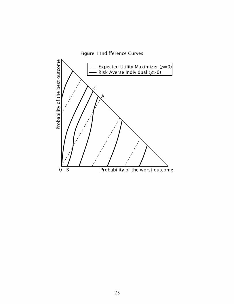
"One-fit-all" formula (23) shows that the model presented in this paper is not radically different from the existing decision theories, at least, when it comes to binary lotteries. However, crucial differences are already apparent when we consider lotteries with three outcomes. The latter case is typically visualized in a Marschak-Machina triangle (e.g., Machina, 1982). The set of all lotteries with up to three outcomes is depicted as an isosceles right triangle
20
with side length one. The vertical side of the triangle shows the probability of the best outcome and the horizontal side shows the probability of the worst outcome.
[INSERT FIGURE 1 HERE]Dashed lines on Figure 1 illustrate indifference curves of an expected
utility maximizer (for whom ρ =0). These curves are parallel straight lines. Solid lines on Figure 1 show indifference curves of a risk averse individual (for whom ρ >0). These curves are convex in the south-east part of the triangle (below line OA) and concave in the north-west part of the triangle (above line OA).
Notably, an indifference curve BC is S-shaped. It is convex in the vicinity of point B and concave—in the vicinity of point C. Such S-shaped indifference curves were discovered in experimental studies (e.g., Bernasconi, 1994). However, few decision theories can generate such curves. In fact, beside the model presented in this paper, there are only two theories able to do this job—rank-dependent utility theory and PRAM. We already discussed how to test our model versus the former. A discriminating test versus the latter is also possible. Our model assumes that individual preferences over lotteries are transitive, while PRAM allows for the possibility of intransitive cycles.
Despite its simplicity, the model presented in this paper can account for a variety of behavioral regularities such as the Allais paradox or the switching behavior in the Samuelson's example. The model has a normative appeal as well. It is rather natural to assume that a decision maker weighs expected utility and utility dispersion in a linear manner. However, the key to success is an appropriate risk measure. Popular ad hoc risk measures, such as the standard deviation or variance, may lead to violations of stochastic dominance (e.g., Borch, 1969). That is why the model presented in this paper is derived from four axioms imposed on a preference relation over lotteries: completeness, transitivity, continuity and the transformed independence axiom. Our derived representation is always compatible with stochastic dominance.
21
AppendixProof of Theorem 2.Consider two arbitrary lotteries L, L´∈ ℒ such that L stochastically
dominates L´. If lottery L stochastically dominates lottery L´ then(A1) ∑x∈X L(x)·g (L) ≥ ∑x∈X L´(x)·g (L), for any function g :X→ℝ such that g(x)≥g(y) if x ≿ y.
Set g (.)=u (.) into (A1) to obtain a standard result: if L stochastically dominates L´ then L yields a higher expected utility, i.e. u (L)≥u (L´). Next, set g (x)=u (x) for all x ∈X such that u (x)<u (L), and set g (x)=u (L) for all x ∈X such that u (x)≥u (L). Inequality (A1) then becomes(A2) ∑x∈X, u(x)<u(L) L(x)·u(x) + u (L)·[1-∑x∈X, u(x)<u(L) L(x)] ≥
≥ ∑x∈X, u(x)<u(L) L´(x)·u(x) + u (L)·[1-∑x∈X, u(x)<u(L) L´(x)]. Since u (L)≥u (L´), it is possible to rewrite inequality (A2) as follows
(A3) u (L)-∑x∈X, u(x)<u(L)L(x)·[u (L)-u(x)]≥u (L´)-∑x∈X, u(x)<u(L´)L´(x)·[u (L´)-u(x)]. If ρ≥0, we can multiply both sides of inequality (A3) by ρ, add u(L)-u(L)
to the left hand side and u (L´)-u (L´) to the right hand side of (A3) and obtain(A4) (ρ -1)·u(L) + u(L) - ρ·r (L) ≥ (ρ -1)·u(L´) + u(L´) - ρ·r (L´).If ρ ≤1 then (ρ -1)·u(L) ≤ (ρ -1)·u(L´) and inequality (A4) may hold only if(A5) u(L) - ρ·r (L) ≥ u(L´) - ρ·r (L´).
Hence, L ≿ L´ due to (1). In the other remaining case, if ρ <0, the proof is similar. First, set g (x)=u (L) for all x ∈X such that u (x)<u (L), and set g (x)=u (x) for all x ∈X such that u (x)≥u (L). Inequality (A1) then becomes(A6) ∑x∈X, u(x)<u(L) L(x)·u(L) + ∑x∈X, u(x)≥u(L) L(x)·u(x) ≥
≥ ∑x∈X, u(x)<u(L) L´(x)·u(L) + ∑x∈X, u(x)≥u(L) L´(x)·u(x). Since u (L)≥u (L´), it is possible to rewrite inequality (A6) as follows
(A7) u (L)+∑x∈X, u(x)<u(L)L(x)·[u (L)-u(x)]≥u (L´)+∑x∈X, u(x)<u(L´)L´(x)·[u (L´)-u(x)]. If ρ <0, it is possible to multiply both sides of inequality (A7) by -ρ
without changing the sign of (A7). Repeating the same manipulation as above (add u (L) - u (L) to the left hand side and u (L´)-u (L´) to the right hand side)
22
yields the following result: (A8) -(1+ρ)·u(L) + u(L) - ρ·r (L) ≥ -(1+ρ)·u(L´) + u(L´) - ρ·r (L´).If ρ ≥-1 then -(1+ρ)·u(L) ≤ -(1+ρ)·u(L´) and inequality (A8) may hold only if(A9) u(L) - ρ·r (L) ≥ u(L´) - ρ·r (L´).
Hence, L ≿ L´ due to (1). Q.E.D.
ReferencesAbdellaoui, Mohammed (2002) "A Genuine Rank-Dependent
Generalization of the von Neumann-Morgenstern Expected Utility Theorem" Econometrica, Vol. 70, pp. 717-736
Allais, Maurice (1953) “Le Comportement de l’Homme Rationnel devant le Risque: Critique des Postulats et Axiomes de l’Ecole Americaine” Econometrica, Vol. 21, pp. 503-546
Bernasconi, Michele (1994) "Nonlinear Preferences and Two-Stage Lotteries: Theories and Evidence" The Economic Journal, Vol. 104, pp. 54-70
Borch, K. (1969) "A Note on Uncertainty and Indifference Curves" The Review of Economic Studies, Vol. 36, No. 1, pp. 1-4
Camerer, Colin and Teck-Hua Ho (1994) “Violations of the Betweenness Axiom and Nonlinearity in Probability” Journal of Risk and Uncertainty, Vol. 8, pp. 167-196
Gul, Faruk (1991) "A Theory of Disappointment Aversion" EconometricaVol. 59, pp. 667-686
Hey, John (2001) “Does repetition improve consistency?” Experimental Economics, Vol. 4, pp. 5-54
Loomes, Graham (2008) “Modelling Choice and Valuation in Decision Experiments”, University of East Anglia working paper
Machina, Mark (1982) ""Expected Utility" Analysis without the Independence Axiom" Econometrica, Vol. 50, pp. 277-324
23
Markowitz, Harry (1952) "Portfolio Selection" The Journal of Finance, Vol. 7, pp. 77-91
Quiggin, John (1981) “Risk perception and risk aversion among Australian farmers” Australian Journal of Agricultural Recourse Economics 25, 160-169
Samuelson, Paul (1963) "Risk and Uncertainty: A Fallacy of Large Numbers" Scientia, Vol. 98, pp. 108-113
Tversky, Amos and Daniel Kahneman (1992) “Advances in Prospect Theory: Cumulative Representation of Uncertainty” Journal of Risk and Uncertainty, Vol. 5, pp. 297-323
von Neumann, John and Oscar Morgenstern (1944) Theory of games and economic behavior Princeton, Princeton University Press