Department of Economics and Business

Aarhus University

Fuglesangs Allé 4

DK-8210 Aarhus V

Denmark

Email: oekonomi@au.dk

Tel: +45 8716 5515

Modeling and Forecasting the Distribution of Energy

Forward Returns

Evidence from the Nordic Power Exchange

Asger Lunde and Kasper V. Olesen

CREATES Research Paper 2013-19

Modeling and Forecasting theDistribution of Energy Forward Returns∗

Evidence from the Nordic Power Exchange

Asger Lunde Kasper V. OlesenAarhus University, Department of Economics and Business & CREATES

July 11, 2014

Abstract

We explore intraday transaction records from NASDAQ OMX Commodities Europe from January

2006 to October 2013. We analyze empirical results for a selection of existing realized measures of

volatility and incorporate them in a Realized GARCH framework for the joint modeling of returns and

realized measures of volatility. An influential bias in these measures is documented, which motivates

the use of a flexible and robust methodology such as the Realized GARCH. Within this framework,

forecasting of the full density for long horizons is feasible, which we pursue. We document variability

in conditional variances over time, which stresses the importance of careful modeling and forecasting

of volatility. We show that improved model fit can be obtained in-sample by utilizing high-frequency

data compared to standard models that use only daily observations. Additionally, we show that the

intraday sampling frequency and method have significant implications for model fit in-sample. Finally,

we consider an extensive out-of-sample exercise to forecast the conditional return distribution. The

out-of-sample results for the Realized GARCH forecasts suggest a limited added value from using

“traditional” realized volatility measures. For the conditional variance, a small gain is found, but for

densities the opposite is the case. We conclude that realized measures of volatility developed in recent

years must be used with caution in this market, and importantly that the use of high-frequency financial

data in this market leaves much room for future research.

Keywords: Volatility, Realized GARCH, High-Frequency Data, Electricity, Power, Forecasting, Realized

Variance, Realized Kernel, Model Confidence Set, Predictive Likelihood

JEL Classification: C10, C22, C53, C58, C80, G40

∗Acknowledgments. Both authors acknowledge support from CREATES - Center for Research in EconometricAnalysis of Time Series (DNRF78), funded by the Danish National Research Foundation, and thank NASDAQOMX Commodities Europe for data access. We also thank the AU Ideas Pilot Center, Stochastic and EconometricAnalysis of Commodity Markets, for financial support. We are grateful to the editor (Torben G. Andersen), theassociate editor, and two referees for a detailed review and comments on a first version of the paper. Also, we thankconference participants at the International Risk Management Conference 2012 in Rome, the CEQURA Conference2012 in Munich, the Energy Finance Conference 2012 in Trondheim, and seminar participants at CREATES forhelpful comments and suggestions. Send correspondence to Asger Lunde, Dept. of Economics and Business, AarhusUniversity, Fuglesangs Allé 4, 8000 Aarhus C, Denmark. E-mail address: alunde@creates.au.dk. All errors are ours.

1 Introduction

Over the past decades, the availability of high-frequency financial data has opened a new

field of research and paved the way for improved measurement, modeling, and forecasting of

volatilities and co-volatilities (see Barndorff-Nielsen and Shephard (2007), Andersen et al. (2009),

and Hansen and Lunde (2011) for recent surveys). Recently, complete records of transaction

prices have become available for a range of derivative contracts that have the system price on

power in the Nordic countries as underlying reference.1 These financial products, and similar in

other regions, have emerged in the aftermath of the liberalizations in numerous countries and

regions. The Nordic countries were the pioneers in the 1990’es, and today the price setting in

all Nordic physical spot markets, with actual delivery of power, is handled by Nord Pool Spot

(NPS). Spot markets have been an active field of study in the academic literature (see Higgs

and Worthington (2008) for a recent survey), whereas the financial markets have caught less

attention. NPS serves as underlying reference for financial futures, forwards, and options traded

on NASDAQ OMX Commodities Europe (NOMXC). The financial contracts were introduced in

1995 motivated by a need for hedging possibilities for market participants exposed to price risk.

We make three main contributions to the literature. First, we are the first to study and use

tick-by-tick data at the highest available frequency in this market. Specifically, we investigate the

liquidity in the NOMXC and conduct an analysis of the most liquid derivative products traded;

the base load forwards (referred to as NOMXC forwards in the following).2 Most previous

research conducted on this data use a daily, or lower, resolution (e.g., Benth and Koekebakker

(2008) or Bauwens et al. (2012)). To the best of our knowledge, only Haugom (2011, 2013) and

Haugom et al. (2011a,b, 2012) have used equally spaced 30-minute intraday prices in this market.

Haugom et al. (2011a,b) calculate the realized variance, the realized bi-power of Barndorff-

Nielsen and Shephard (2004), and the realized outlyingness co-variation of Boudt et al. (2011).

Using these measures in different time-series models they compare the ability to forecast one-

step ahead in-sample with that of traditional GARCH models with and without explanatory

market measures. We investigate the added value from sampling at higher frequencies, which

in many cases are a necessity for the validity of a realized volatility measure (i.e., 30-minute

sampling is often too low as also pointed out in both Barndorff-Nielsen and Shephard (2004)

and Boudt et al. (2011)). Also, as we will show, one must be cautious with the evaluation of

models using different proxies for the true, unobservable volatility due to an inherent bias in

“traditional” realized volatility measures.3

1We refer to “electric power” as “power” throughout.2Strictly speaking, the contracts are swaps, as they specify an exchange of a fixed cash flow (the forward price)

for a floating cash flow (the underlying reference) over a settlement period. We follow the NOMXC terminology.3For example, Haugom et al. (2011a) use the 30-minute realized variance as proxy for the true unobservable

volatility. In Section 3.4, we show that the realized variance is a biased proxy in this market.

2

Second, we show that the inclusion of intraday information and the use of novel econometric

methodologies improve the modeling and forecasting of volatilities in an important branch

of the energy markets. We utilize the information contained in realized measures of volatility

to estimate the conditional variance of daily returns within the Realized GARCH framework

of Hansen et al. (2012a). We find that Realized GARCH models that utilize the information

in realized ex-post measures of volatility outperform the benchmark GARCH type models in-

sample. The Realized GARCH framework is itself dependent on the realized volatility measure

being used. This is used to provide guidance for the optimal sampling frequency and method.

Furthermore, in some cases even better in-sample performance can be obtained by including

multiple realized measures of volatility.

Third, we are the first to consider empirical out-of-sample forecasting in the Realized GARCH

framework beyond one day. We present out-of-sample forecasts up to 40 business days of both

the conditional return variance and return density. We find that the superior performance in-

sample does not fully manifest itself out-of-sample. The added value is limited for volatility

forecasts and non-existing for density forecasts.

Overall, our work shows that by means of the Realized GARCH framework one can in a

simple way obtain more precise volatility estimates and short term predictions for the NOMXC

forwards, but that the use of realized measures of volatility should be tailored to the market.

In our opinion, power markets are distinct and require further analysis on their own. The

importance is demonstrated in for example Geman and Roncoroni (2006), Escribano et al. (2011),

and Veraart and Veraart (2013) for spot prices. Contrasting these studies, our data set is from the

derivatives market. We expect, and find, that these prices behave more as traditional financial

assets than the spot price that has a very special structure in power markets (see e.g.Veraart

and Veraart (2013)). Derivatives on flow commodities, such as power, are often settled against

an average of the spot price over a specified delivery period. That is easily contracted for

futures and forwards contracts and in the option space classified as Asian options. Consequently,

futures and forwards stop trading before the delivery period, which creates the need for rollover

between consecutive contracts in order to analyze continual time series.4 Intraday, the derivative

contracts trade as in other markets. This creates potential also for speculation. For the specific

contracts analyzed in this paper the trading activity counts almost 1, 000, 000 transactions over

our sample period from January 2006 to October 2013. Our results are of major importance

for producers, utility companies, and other participants in the power sector. These agents are

exposed to the physical spot market for power, and the financial products traded on NOMXC

provide important tools for hedging the risk inherent. The financial products provide protection

to rapidly changing prices and to others they are vehicles for portfolio diversification. In active

risk and portfolio management, volatility estimates, and in some situations the full return

4A discussion of this topic can be found in the Online Appendix.

3

distribution, are needed for traditional Markowitz portfolio theory, calculation of hedge ratios,

value at risk (VaR) estimates, and so forth. Further, volatility estimates are needed in the pricing

of options written on these products, which trade both on NOMXC and over-the-counter.

The paper is organized as follows. Section 2 introduces the history of, and the products

traded on, NOMXC and related markets. Section 3 presents the data and how how we our handle

it. Then it briefly introduces the realized volatility measures used, investigate their properties,

and analyzes the continual series at the daily frequency. Section 4 presents the econometric

methodology used, the Realized GARCH framework, and Section 5 presents estimation results.

In Section 6 we perform regular and bootstrapped rolling-window forecasting and evaluate

volatility predictions from the models using Mincer-Zarnowitz type regressions, and using the

predictive likelihood for evaluation of the full density. Section 7 concludes.

2 The Financial Market for Nordic Power

Wholesale power markets were liberalized in numerous countries beginning in the early 1990s.

The non-storability of power creates a need for real-time balancing of locational supply and

demand, which in most countries rely on an independent transmission system operator (ITSO).5

The ITSOs are non-commercial monopolies that operate the high-voltage grids and secure the

supply of power through the regulating markets.6 In regulating markets, prices are volatile

and most market participants seek to forecast production or demand in order to take positions

beforehand, bilaterally or through pools. Optimally, only discrepancies between the expectations

and actual needs are settled in the regulating market. NPS is a pool and operates a day-ahead

double auction market, Elspot, where market participants submit supply and demand no later

than noon the day before the energy is delivered to the grid. A market system clearing price for

all hours in the following day is calculated and announced.7 The system clearing price from the

NPS is the underlying reference price for a range of derivative contracts traded on NOMXC,

where the participants contract for the delivery of power ranging from a few days to years

ahead.8 NOMXC is exchange-based, but also bilateral or broker-based OTC trades are registered,

and for some products one or more market makers post two-sided quotes in the order book.

We consider the set of base load forward contracts traded on NOMXC with the NPS system

5In the Nordic countries the ITSOs are Energinet.dk, Statnett, Svenska Kraftnät, and Fingrid. The ITSOs maintainthe system and manages provision, contracting, and infrastructure for all needed activities.

6Actual consumption may exceed production and the frequency of the alternating current falls below the target(50 Hz in this region). The ITSO procures “up regulating” (as opposed to “down regulating” in the opposite case).

7Furthermore, due to grid bottlenecks, bidding areas develop such that different regions in the Nordic countriesare exposed to different prices in some hours. To further reduce the exposure to the balancing market, a cross-borderintraday market, Elbas, opens two hours after the closure of NPS and closes one hour prior to the operation hour.The organization of physical exchanges varies between regions, and we limit ourselves to this brief and simplifiedexposition of the Nordic market. See www.nordpoolspot.com for details.

8Originally introduced as Eltermin by Nord Pool in late 1995, which among other entities was acquired byNASDAQ OMX in 2008 and merged into NOMXC, the exchange is among the leading and most liquid exchanges inthe world for financial derivatives on power.

4

clearing price as the underlying reference. This is by far the most liquid subset of the traded

products. Market participants enter into contracts with a specified delivery period; monthly,

quarterly or yearly, and contracts kept until expiry are settled financially on every clearing

day during this period. No physical supply or receipt of power occurs. Prices are quoted in

EUR/MWh, and each contract specifies delivery of a continuous flow of power during the

delivery period of 1MW.9 Monthly contracts trade until the last trading day before the specified

delivery period, and settlement is spot reference cash on every clearing day during the delivery

period. Quarterly contracts are cascaded from yearly contracts and into monthly contracts

on the last trading day before the specified delivery period.10 All settling of accounts takes

place through NOMXC, and the two parties involved do not know each others identity, but

the settling is guaranteed by NOMXC. Swedish Vattenfall acts as market maker on base load

forward contracts with commitments to continuously quote buy and sell prices in the order

book within a maximum spread determined by volatility and price levels.11

3 Data

We have available transaction data for all contracts traded on NOMXC in the period 2 January

2006 to 25 October 2013 delivering 1966 distinct trading days. The information contained in the

data files and our data handling is relegated to the Online Appendix. The left part of Table 1

sorts according to deal source and category. The most traded contracts are among the base load

futures and forwards. The trade in peak loads is limited, and also options are rarely traded. We

exclude the OTC trades as the time stamps are often imprecise. This makes them unfit for an

intraday analysis. Also, the transaction prices of OTC trades are often unreliable.12 Focusing

on exchange-traded base load futures and forwards alone leaves 960, 256 transactions. From

the right part of Table 1 quarterly contracts are seen to be the most traded, and the futures

are the least traded. With liquidity deemed important, we limit ourselves to consider the most

traded contracts, the forwards. In the period 2 January 2006 to 25 October 2013, the specifications

(delivery period, contract size, currency quote, etc.) of the forwards have remained unchanged.

Further, the opening hours of the exchange have remained the same and no half trading days

are present.

9The structure of traded derivatives has changed several times since the market opening but has remainedunchanged since January 2006. Also, contracts with a delivery period prior to 2006 were quoted in NOK/MWh.

10Yearly contracts are cascaded into quarterly contracts three trading days prior to the delivery period.11See NASDAQ OMX Commodities (2011a) for details on traded products, and NASDAQ OMX Commodi-

ties (2011b) and NASDAQ OMX Commodities (2011c) for details on trading and clearing on NOMXC. Also, seenordpoolspot.com, nasdaqomxcommodities.com, and eex.com for further details on this Section.

12As an example, the ENOMMAR-08 contract was traded to 1 EUR/MWh and 528.6 EUR/MWh at the same timeon 11 February 2008 implying that the trade may have been a part of a bigger deal.

5

Table 1: Overview of transactions in derivative contracts traded on NOMXC.

Product OTC ExchangeSpecification Transactions Transactions

Base 271, 875 951, 654BaseDay 443 8, 602

CfD 30, 437 17, 941Option 4, 947 23Peak 36 54

307, 738 978, 274

Length ofDelivery Period Transactions

Day (future) 8, 602Week (future) 47, 337

Month (forward) 148, 310Quarter (forward) 568, 275

Year (forward) 187, 732960, 256

The sample period is 02 January 2006 to 25 October 2013. Left part: Number of transactions sorted according toDealSource (OTC: Over The Counter, Exchange) and MainCategory (Base: forward and future base load contracts witha weekly, monthly, quarterly, or yearly delivery period, BaseDay: future base load contracts with a daily deliveryperiod, CfD: Contract for Differences, Option: European call and put (written on quarterly forwards), Peak: forwardand future peak load contracts with a weekly, monthly, quarterly, or yearly delivery period). Right part: Number ofexchange transactions in future and forward base load contracts sorted according to length of delivery period.

3.1 Realized Measures of Volatility

We consider a collection of realized measures of volatility, which we briefly introduce in this

section. We follow the implementation of the authors of the original papers as closely as possible

and omit detailed descriptions of each estimator in the interest of space. Intraday log-returns are

defined from the log-prices at time t, p?t , by

r?tj,m:= p?tj,m

− p?tj−1,m, j = 1, . . . m,

and calculated from intraday log-prices spanning the period 8:00 AM to 15:30 PM (the hours

the exchange is open). Here, subscript index j refers to the (possibly) irregular spaced sequence

of the raw data series at day t, i.e., we partition the interval [0, T] into m sub-intervals. The

standard realized variance of p? is defined as

RV(m)? :=

m

∑j=1

(r?j,m)2

,

which yields a precise estimate of volatility when prices are observed continuously and without

measurement error (see, e.g., Protter (2005) and Barndorff-Nielsen and Shephard (2002)). RV(m)?

is ideal, but infeasible as p? is latent. For the observable price process, p, we observe on day t the

RV based on m intraday returns, which is generally inconsistent for the quadratic variation of the

latent price (see, e.g., Zhang et al. (2005)). We consider various versions of RV(m) := ∑mj=1(rj,m)2 ,

where rj,m is the observed intraday return, that is a noisy proxy of r?j,m. We take tj,m, j = 0, . . . , m,

to be equidistant in calender time, i.e., calendar time sampling (CTS), which we implement using

previous-tick interpolation (see Hansen and Lunde (2006)). Under CTS, we write RV(x sec), when

6

δj,m = x seconds, and we make use of simple one-minute sub-sampling, which is indicated in the

subscript, e.g., RV(300 sec)ss .13 Finally, we consider the realized variance based on all tick-by-tick

returns, RV(tick).

To the best of our knowledge, the sensitivity of the realized variance to market frictions has

not been studied for NOMXC forwards. Thus, we include the realized kernels of Barndorff-

Nielsen et al. (2011), which is a broad set of estimators designed to be robust to most types of

frictions. In the univariate case with time gap δm > 0 they are given by

K (pδm) =m

∑h=−m

k(

hH + 1

)Γh, Γh =

m

∑j=|h|+1

rtj,m rt(j−h),m ,

where k (x), for x ∈ R, is a non-stochastic weight function and Γh is the hth realized auto-

covariance. We follow the suggestions in Barndorff-Nielsen et al. (2011) with respect to the

jittering of the initial and final time points each day, the selection of the optimal bandwidth, H,

for the recommended “non-flat-top Parzen” kernel as the choice of k (x), and for the estimation

of the noise-to-signal-ratio ξ2 by ξ2 =(RV(tick)/(2·N))

RV(1800 sec) .14 We refer to this simply as the realized

kernel (RK). All realized volatility measures were based on cleaned transactions data following

Barndorff-Nielsen et al. (2009). Section 3.3 presents stylized facts for the realized volatility

measures.

3.2 Stylized Facts for the Price Process at the Daily Frequency

The existing literature on modeling and forecasting volatility in power futures and forwards

has mainly utilized observations at a daily frequency (see e.g. references in the introduction

and also Malo and Kanto (2006), Benth et al. (2008a), and Pen and Sévi (2010)). The classical

GARCH framework often utilizes daily returns (or lower frequencies) to extract information

about the current and future level of volatility. To motivate the application of GARCH models

we document in this section the common stylized facts of financial series at the daily frequency:

unpredictability of returns, volatility clustering, leptokurtosis, asymmetries, and so forth. In the

Realized GARCH framework we use roct and rcc

t to denote open-to-close and close-to-close daily

returns at day t, respectively, with realized measures of volatility denoted by xt. Open-to-close

returns are the daily changes in the logarithm of the first and last transaction price each day, and

close-to-close returns at time t are the daily changes in the logarithm of the last transaction price

at time t− 1 and t. The information set is then given by Ft ={

roct , rcc

t , xt, roct−1, rcc

t−1, xt−1, . . .}

,

which is richer than in the conventional GARCH framework.

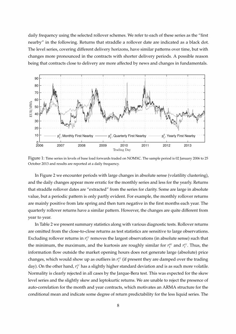
In Figure 1 we present the continual monthly, quarterly, and yearly series in levels, and in

Figure 2 the daily changes in the logarithm of these, i.e., the close-to-close returns, all at the

13See the Online Appendix for an explanation of our use of sub-sampling.14We set H = c?ξ

4/5m3/5, where c? ={

k′′ (0) /k0,0•}1/5

and k0,0• :=

∫ 10 k (x)2 dx.

7

daily frequency using the selected rollover schemes. We refer to each of these series as the “first

nearby” in the following. Returns that straddle a rollover date are indicated as a black dot.

The level series, covering different delivery horizons, have similar patterns over time, but with

changes more pronounced in the contracts with shorter delivery periods. A possible reason

being that contracts close to delivery are more affected by news and changes in fundamentals.

2006 2007 2008 2009 2010 2011 2012 20130

10

20

30

40

50

60

70

80

90

Trading Day

EUR/M

Wh

pc

t, Monthly First Nearby p

c

t, Quarterly First Nearby p

c

t, Yearly First Nearby

Figure 1: Time series in levels of base load forwards traded on NOMXC. The sample period is 02 January 2006 to 25October 2013 and results are reported at a daily frequency.

In Figure 2 we encounter periods with large changes in absolute sense (volatility clustering),

and the daily changes appear more erratic for the monthly series and less for the yearly. Returns

that straddle rollover dates are “extracted” from the series for clarity. Some are large in absolute

value, but a periodic pattern is only partly evident. For example, the monthly rollover returns

are mainly positive from late spring and then turn negative in the first months each year. The

quarterly rollover returns have a similar pattern. However, the changes are quite different from

year to year.

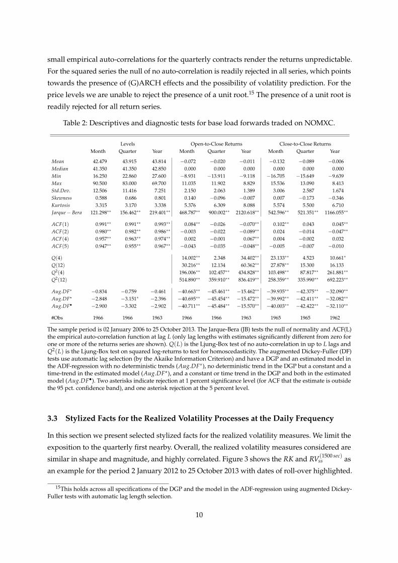
In Table 2 we present summary statistics along with various diagnostic tests. Rollover returns

are omitted from the close-to-close returns as test statistics are sensitive to large observations.

Excluding rollover returns in rcct removes the largest observations (in absolute sense) such that

the minimum, the maximum, and the kurtosis are roughly similar for roct and rcc

t . Thus, the

information flow outside the market opening hours does not generate large (absolute) price

changes, which would show up as outliers in rcct (if present they are damped over the trading

day). On the other hand, rcct has a slightly higher standard deviation and is as such more volatile.

Normality is clearly rejected in all cases by the Jarque-Bera test. This was expected for the skew

level series and the slightly skew and leptokurtic returns. We are unable to reject the presence of

auto-correlation for the month and year contracts, which motivates an ARMA structure for the

conditional mean and indicate some degree of return predictability for the less liquid series. The

8

2006 2007 2008 2009 2010 2011 2012 2013−15

−10

−5

0

5

10

15

Trading Day

Chan

ge(inpercent)

rcc

t, Monthly First Nearby Rollover returns

2006 2007 2008 2009 2010 2011 2012 2013−15

−10

−5

0

5

10

15

Trading Day

Chan

ge(inpercent)

rcc

t, Quarterly First Nearby Rollover returns

2006 2007 2008 2009 2010 2011 2012 2013−15

−10

−5

0

5

10

15

Trading Day

Chan

ge(inpercent)

rcc

t, Yearly First Nearby Rollover returns

Figure 2: Log-returns of base load forwards traded on NOMXC. The sample period is 02 January 2006 to 25 October2013, and results are reported at a daily frequency. The top row presents the monthly first nearby, the middle row thequarterly first nearby, and the bottom row the yearly first nearby. Returns that straddle a rollover date are indicated asa black dot (some observations are outside the chosen range).

9

small empirical auto-correlations for the quarterly contracts render the returns unpredictable.

For the squared series the null of no auto-correlation is readily rejected in all series, which points

towards the presence of (G)ARCH effects and the possibility of volatility prediction. For the

price levels we are unable to reject the presence of a unit root.15 The presence of a unit root is

readily rejected for all return series.

Table 2: Descriptives and diagnostic tests for base load forwards traded on NOMXC.

Levels Open-to-Close Returns Close-to-Close ReturnsMonth Quarter Year Month Quarter Year Month Quarter Year

Mean 42.479 43.915 43.814 −0.072 −0.020 −0.011 −0.132 −0.089 −0.006Median 41.350 41.350 42.850 0.000 0.000 0.000 0.000 0.000 0.000Min 16.250 22.860 27.600 −8.931 −13.911 −9.118 −16.705 −15.649 −9.639Max 90.500 83.000 69.700 11.035 11.902 8.829 15.536 13.090 8.413Std.Dev. 12.506 11.416 7.251 2.150 2.063 1.389 3.006 2.587 1.674Skewness 0.588 0.686 0.801 0.140 −0.096 −0.007 0.007 −0.173 −0.346Kurtosis 3.315 3.170 3.338 5.376 6.309 8.088 5.574 5.500 6.710Jarque− Bera 121.298∗∗ 156.462∗∗ 219.401∗∗ 468.787∗∗ 900.002∗∗ 2120.618∗∗ 542.596∗∗ 521.351∗∗ 1166.055∗∗

ACF(1) 0.991∗∗ 0.991∗∗ 0.993∗∗ 0.084∗∗ −0.026 −0.070∗∗ 0.102∗∗ 0.043 0.045∗∗

ACF(2) 0.980∗∗ 0.982∗∗ 0.986∗∗ −0.003 −0.022 −0.089∗∗ 0.024 −0.014 −0.047∗∗

ACF(4) 0.957∗∗ 0.963∗∗ 0.974∗∗ 0.002 −0.001 0.067∗∗ 0.004 −0.002 0.032ACF(5) 0.947∗∗ 0.955∗∗ 0.967∗∗ −0.043 −0.035 −0.048∗∗ −0.005 −0.007 −0.010

Q(4) 14.002∗∗ 2.348 34.402∗∗ 23.133∗∗ 4.523 10.661∗

Q(12) 30.216∗∗ 12.134 60.362∗∗ 27.878∗∗ 15.300 16.133Q2(4) 196.006∗∗ 102.457∗∗ 434.828∗∗ 103.498∗∗ 87.817∗∗ 261.881∗∗

Q2(12) 514.890∗∗ 359.910∗∗ 836.419∗∗ 258.359∗∗ 335.990∗∗ 692.223∗∗

Aug.DF∗ −0.834 −0.759 −0.461 −40.663∗∗ −45.461∗∗ −15.462∗∗ −39.935∗∗ −42.375∗∗ −32.090∗∗

Aug.DF? −2.848 −3.151∗ −2.396 −40.695∗∗ −45.454∗∗ −15.472∗∗ −39.992∗∗ −42.411∗∗ −32.082∗∗

Aug.DF• −2.900 −3.302 −2.902 −40.711∗∗ −45.484∗∗ −15.570∗∗ −40.003∗∗ −42.422∗∗ −32.110∗∗

#Obs 1966 1966 1963 1966 1966 1963 1965 1965 1962

The sample period is 02 January 2006 to 25 October 2013. The Jarque-Bera (JB) tests the null of normality and ACF(L)the empirical auto-correlation function at lag L (only lag lengths with estimates significantly different from zero forone or more of the returns series are shown). Q(L) is the Ljung-Box test of no auto-correlation in up to L lags andQ2(L) is the Ljung-Box test on squared log-returns to test for homoscedasticity. The augmented Dickey-Fuller (DF)tests use automatic lag selection (by the Akaike Information Criterion) and have a DGP and an estimated model inthe ADF-regression with no deterministic trends (Aug.DF∗), no deterministic trend in the DGP but a constant and atime-trend in the estimated model (Aug.DF?), and a constant or time trend in the DGP and both in the estimatedmodel (Aug.DF•). Two asterisks indicate rejection at 1 percent significance level (for ACF that the estimate is outsidethe 95 pct. confidence band), and one asterisk rejection at the 5 percent level.

3.3 Stylized Facts for the Realized Volatility Processes at the Daily Frequency

In this section we present selected stylized facts for the realized volatility measures. We limit the

exposition to the quarterly first nearby. Overall, the realized volatility measures considered are

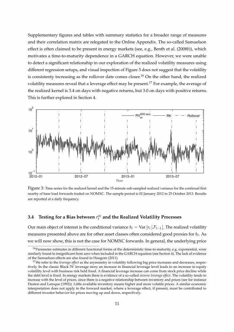
similar in shape and magnitude, and highly correlated. Figure 3 shows the RK and RV(1500 sec)ss as

an example for the period 2 January 2012 to 25 October 2013 with dates of roll-over highlighted.

15This holds across all specifications of the DGP and the model in the ADF-regression using augmented Dickey-Fuller tests with automatic lag length selection.

10

Supplementary figures and tables with summary statistics for a broader range of measures

and their correlation matrix are relegated to the Online Appendix. The so-called Samuelson

effect is often claimed to be present in energy markets (see, e.g., Benth et al. (2008b)), which

motivates a time-to-maturity dependence in a GARCH equation. However, we were unable

to detect a significant relationship in our exploration of the realized volatility measures using

different regression setups, and visual inspection of Figure 3 does not suggest that the volatility

is consistenty increasing as the rollover date comes closer.16 On the other hand, the realized

volatility measures reveal that a leverage effect may be present.17 For example, the average of

the realized kernel is 3.4 on days with negative returns, but 3.0 on days with positive returns.

This is further explored in Section 4.

2012−01 2012−07 2013−01 2013−0710

−1

100

101

102

Date

RV(900 sec)

ssRK Rollover

Figure 3: Time series for the realized kernel and the 15-minute sub-sampled realized variance for the continual firstnearby of base load forwards traded on NOMXC. The sample period is 02 January 2012 to 25 October 2013. Resultsare reported at a daily frequency.

3.4 Testing for a Bias between roct and the Realized Volatility Processes

Our main object of interest is the conditional variance ht = Var [rt |Ft−1 ]. The realized volatility

measures presented above are for other asset classes often considered good proxies for ht. As

we will now show, this is not the case for NOMXC forwards. In general, the underlying price

16Parameter estimates in different functional forms of the deterministic time-to-maturity, e.g. exponential, weresimilarly found to insignificant from zero when included in the GARCH-equation (see Section 4). The lack of evidenceof the Samuelson effects are also found in Haugom (2011).

17We refer to the leverage effect as the asymmetry in volatility following big price increases and decreases, respec-tively. In the classic Black 76’ leverage story an increase in financial leverage level leads to an increase in equityvolatility level with business risk held fixed. A financial leverage increase can come from stock price decline whilethe debt level is fixed. In energy markets there is evidence of a so-called inverse leverage effect. The volatility tends toincrease with the level of prices, since there is a negative relationship between inventory and prices (see for instanceDeaton and Laroque (1992)). Little available inventory means higher and more volatile prices. A similar economicinterpretation does not apply in the forward market, where a leverage effect, if present, must be contributed todifferent investor behavior for prices moving up and down, respectively.

11

process and market microstructure noise is not well understood for NOMXC forwards, and

we are concerned that the direct use of them in traditional time-series models (as it is done

in e.g. Haugom et al. (2011a,b, 2012)) limits the validity of several central results. Testing the

many different assumptions and building modified realized measures for this particular market

is not the purpose of this paper. We seek to utilize the information contained in traditional

realized measures of volatility without jeopardizing the validity of our results. The methodology

presented in Section 4 achieves this, and the realized kernel is used as a robust measure that uses

all available tick-by-tick data. To evaluate model performance in Section 6 only a bias between

roct and the realized volatility processes is a concern. Following Hansen and Lunde (2005), Table

3 presents regression results for selected kitchen sink regressions of the form

(roct )2 − xt = β′Zt + ut.

Panel A uses only a constant (i.e. Zt = 1) as regressor and confirms the existence of a bias. (roct )2 is

a noisy, but an unbiased measure of hoct . Thus, Panel A clearly reveals that xt is a biased measure

of hoct . Panel B has Zt =

(Dmon,t, Dtue,t, Dwed,t, Dthu,t, Dfri,t

), which consists of five weekday

indicator functions. Panel B reveals that the bias is most severe on Mondays. For most realized

measures the bias is decreasing Monday-Thursday and slightly higher on Fridays relative to

Thursdays. Panel C has Zt =(

QACF1,t , QACF

2,t , . . . , QACF5,t

), where we define QACF

j,t = 1{ACF(1)t∈Ij}for j = 1, . . . , 5, t = 1, . . . T, and I1, I2, I3, I4, and I5 is the segmentation of support for the first-

order auto-correlation of intraday (non-zero) returns using the 20%, 40%, 60%, and 80% empirical

quantiles.18 Panel C reveals interesting differences among the realized measures. The realized

kernel eliminated the bias for the largest positive auto-correlation, but suffers in the mid-range

like the others. In particular, the bias is large between the 60% and 80% quantiles. RV(tick) has

the largest bias among all measures except for the days with the smallest (most negative) auto-

correlation. The realized variances are similar with sub-sampling, and the bias gets smaller for

more sparse sampling as expected. Next, Panel D has Zt =(

QNobs1,t , QNobs

2,t , . . . , QNobs5,t

), where we

define QNobsj,t = 1{Nobst∈Ij} for j = 1, . . . , 5, t = 1, . . . T, and I1, I2, . . ., and I5, is the segmentation

of support for the number of intraday transactions using similar quantiles as before. Interestingly,

the bias is larger for days with more observations, where we expected the realized measures

to perform better. Finally, Panel E has Zt =(

Q|roc|

1,t , Q|roc|

2,t , . . . , Q|roc|

10,t

), where we define Q|r

oc|j,t =

1{|roc|t∈Ij} for j = 1, . . . , 10, t = 1, . . . T, and I1, I2, . . ., and I10 is the segmentation of support

for the daily absolute open-to-close returns. A bias arise for returns around zero and for large

returns.

It is beyond the scope of this paper to go into more detail. We provide Table 3 for further

research. Also, Figure 4 illustrates the intraday price paths for two days with a large transaction

count, and Figures A.3-A.5 in the Online Appendix shows the time-span of each trading day,

18In Panel B, the quantiles are −0.070, 0.014, 0.082, and 0.171. In Panel D, the quantiles are 113, 156, 204, and 269.

12

Table 3: Kitchen sink regressions for the bias (roct )2 − xt.

Measure: RK RV RVss RVss RVss RV RV RV RV RVFrequency: Tick Tick 5-min 15-min 30-min 5-min 15-min 30-min 60-min 120-min

Panel A: Regression on a Constant

β 1.082(0.000)

1.707(0.000)

0.997(0.000)

0.921(0.000)

1.040(0.000)

0.955(0.000)

0.750(0.000)

0.835(0.000)

0.801(0.000)

0.686(0.000)

Panel B: Regression on Weekday Dummies

β1, Dmon,t 3.200(0.000)

3.944(0.000)

3.181(0.000)

3.048(0.000)

3.080(0.000)

3.094(0.000)

2.816(0.000)

2.738(0.000)

2.535(0.000)

2.248(0.000)

β2, Dtue,t 0.838(0.022)

1.480(0.000)

0.723(0.053)

0.654(0.068)

0.790(0.019)

0.681(0.059)

0.482(0.171)

0.699(0.041)

0.703(0.033)

0.469(0.133)

β3, Dwed,t 0.806(0.029)

1.485(0.000)

0.673(0.062)

0.596(0.097)

0.764(0.032)

0.637(0.081)

0.471(0.194)

0.530(0.155)

0.466(0.199)

0.437(0.160)

β4, Dthu,t 0.133(0.707)

0.769(0.027)

0.092(0.778)

0.026(0.934)

0.118(0.694)

0.099(0.763)

−0.089(0.767)

−0.060(0.813)

−0.048(0.870)

0.023(0.930)

β5, D f ri,t 0.492(0.032)

0.918(0.000)

0.379(0.109)

0.341(0.133)

0.504(0.023)

0.324(0.173)

0.128(0.561)

0.321(0.132)

0.398(0.049)

0.297(0.096)

Panel C: Regression on Intraday Autocorrelation Quantiles

β1, QACF1,t 0.809

(0.029)0.484(0.196)

0.381(0.267)

0.519(0.118)

0.670(0.030)

0.402(0.237)

0.375(0.207)

0.408(0.110)

0.631(0.044)

0.512(0.039)

β2, QACF2,t 0.580

(0.113)0.639(0.080)

0.453(0.203)

0.491(0.169)

0.555(0.109)

0.455(0.200)

0.452(0.211)

0.520(0.120)

0.648(0.041)

0.572(0.031)

β3, QACF3,t 0.586

(0.079)0.763(0.032)

0.534(0.106)

0.474(0.138)

0.484(0.116)

0.484(0.144)

0.361(0.262)

0.368(0.241)

0.214(0.484)

0.024(0.933)

β4, QACF4,t 1.000

(0.040)1.525(0.003)

1.008(0.037)

0.967(0.037)

1.057(0.015)

1.005(0.037)

0.858(0.064)

0.942(0.034)

0.833(0.053)

0.986(0.004)

β5, QACF5,t 0.055

(0.902)1.327(0.009)

0.356(0.434)

0.063(0.888)

0.125(0.769)

0.292(0.526)

−0.073(0.866)

−0.145(0.733)

−0.130(0.759)

−0.213(0.581)

Panel D: Regression on Intraday Transaction Counts

β1, QNobs1,t 0.091

(0.683)0.273(0.267)

0.050(0.830)

0.003(0.991)

0.124(0.587)

0.052(0.812)

−0.076(0.738)

−0.032(0.892)

0.036(0.864)

0.135(0.414)

β2, QNobs2,t 0.174

(0.399)0.517(0.019)

0.138(0.506)

0.082(0.679)

0.218(0.271)

0.118(0.568)

−0.102(0.587)

0.037(0.830)

0.109(0.517)

0.198(0.151)

β3, QNobs3,t 0.105

(0.711)0.143(0.633)

0.034(0.906)

0.131(0.633)

0.144(0.594)

−0.006(0.985)

0.144(0.597)

0.109(0.672)

0.027(0.914)

0.027(0.906)

β4, QNobs4,t 0.854

(0.157)1.354(0.033)

0.941(0.114)

0.779(0.171)

0.768(0.144)

0.946(0.105)

0.739(0.199)

0.853(0.112)

0.838(0.113)

0.649(0.193)

β5, QNobs5,t 2.660

(0.005)3.124(0.002)

2.457(0.009)

2.373(0.008)

2.289(0.007)

2.433(0.008)

2.377(0.007)

2.077(0.016)

1.822(0.030)

1.144(0.118)

Panel E: Regression on Daily Returns

β1, Qroct

1,t 1.721(0.002)

2.146(0.000)

1.681(0.028)

1.570(0.034)

1.481(0.011)

1.726(0.037)

1.132(0.034)

1.082(0.014)

0.922(0.022)

0.543(0.012)

β2, Qroct

2,t −0.890(0.085)

−0.854(0.110)

−0.924(0.209)

−0.964(0.179)

−1.091(0.051)

−0.907(0.259)

−1.356(0.008)

−1.370(0.001)

−1.375(0.000)

−1.063(0.000)

β3, Qroct

3,t −0.885(0.123)

−0.868(0.132)

−0.902(0.244)

−0.888(0.248)

−1.025(0.099)

−0.862(0.302)

−1.218(0.035)

−1.232(0.009)

−1.193(0.006)

−0.769(0.000)

β4, Qroct

4,t −0.442(0.396)

−0.335(0.530)

−0.422(0.568)

−0.394(0.582)

−0.481(0.384)

−0.385(0.633)

−0.737(0.153)

−0.821(0.057)

−0.696(0.073)

−0.758(0.000)

β5, Qroct

5,t −0.474(0.400)

−0.389(0.495)

−0.479(0.535)

−0.470(0.532)

−0.505(0.392)

−0.447(0.594)

−0.802(0.142)

−0.801(0.072)

−0.876(0.039)

−0.710(0.001)

β6, Qroct

6,t −0.933(0.057)

−0.738(0.160)

−1.011(0.161)

−0.973(0.164)

−0.721(0.175)

−1.084(0.170)

−0.708(0.136)

−0.529(0.156)

−0.376(0.263)

−0.060(0.631)

β7, Qroct

7,t 0.155(0.393)

0.519(0.003)

0.057(0.787)

0.010(0.963)

0.155(0.455)

0.013(0.952)

−0.091(0.670)

−0.036(0.861)

0.088(0.665)

0.172(0.389)

β8, Qroct

8,t 1.150(0.000)

1.871(0.000)

1.156(0.000)

1.076(0.000)

1.070(0.000)

1.135(0.000)

1.037(0.000)

0.901(0.001)

0.504(0.114)

0.391(0.195)

β9, Qroct

9,t 2.782(0.000)

4.062(0.000)

2.868(0.000)

2.842(0.000)

3.008(0.000)

2.746(0.000)

2.580(0.000)

2.660(0.000)

2.512(0.000)

2.294(0.000)

β10, Qroct

10,t 18.10(0.000)

20.08(0.000)

18.02(0.000)

17.26(0.000)

16.75(0.000)

17.84(0.000)

16.48(0.000)

16.01(0.000)

14.86(0.000)

11.33(0.000)

Parameter estimates for four kitchen sink regressions with p-values in parenthesis. Estimates that are significantlydifferent from zero at the 5% level is marked in gray. The sample period is 02 January 2006 to 25 October 2013.

13

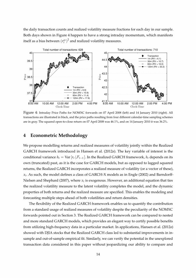
the daily transaction counts and realized volatility measure fractions for each day in our sample.

Both days shown in Figure 4 happen to have a strong intraday momentum, which manifests

itself as a bias between (roct )2 and realized volatility measures.

8:00 AM 10:00 AM 12:00 AM 2:00 PM 4:00 PM37

37.5

38

38.5

39

39.5

40

Clock-Time

Price

Total number of transactions: 628

Transaction

1m (RV = 6.9)

30m (RV = 10.9)

60m (RV = 11.4)

120m (RV = 17.8)

8:00 AM 10:00 AM 12:00 AM 2:00 PM 4:00 PM41.5

42

42.5

43

43.5

44

44.5

45

Clock-Time

Price

Total number of transactions: 710

Transaction

1m (RV = 6.1)

30m (RV = 10.7)

60m (RV = 16.0)

120m (RV = 33.2)

Figure 4: Intraday Price Paths for NOMXC forwards on 07 April 2008 (left) and 14 January 2010 (right). Alltransactions are illustrated in black, and the price paths resulting from four different calendar-time sampling schemesare in gray. The squared open-to-close return on 07 April 2008 was 46.1%, and on 14 January 2010 it was 36.2%.

4 Econometric Methodology

We propose modelling returns and realized measures of volatility jointly within the Realized

GARCH framework introduced in Hansen et al. (2012a). The key variable of interest is the

conditional variance ht = Var [rt |Ft−1 ]. In the Realized GARCH framework, ht depends on its

own (truncated) past, as it is the case for GARCH models, but as opposed to lagged squared

returns, the Realized GARCH incorporates a realized measure of volatility (or a vector of these),

xt. As such, the model defines a class of GARCH-X models as in Engle (2002) and Barndorff-

Nielsen and Shephard (2007), where xt is exogenous. However, an additional equation that ties

the realized volatility measure to the latent volatility completes the model, and the dynamic

properties of both returns and the realized measure are specified. This enables the modeling and

forecasting multiple steps ahead of both volatilities and return densities.

The flexibility of the Realized GARCH framework enables us to quantify the contribution

from a standard usage of realized measures of volatility despite the peculiarity of the NOMXC

forwards pointed out in Section 3. The Realized GARCH framework can be compared to nested

and more standard GARCH models, which provides an elegant way to certify possible benefits

from utilizing high-frequency data in a particular market. In applications, Hansen et al. (2012a)

showed with DJIA stocks that the Realized GARCH class led to substantial improvements in in-

sample and out-of-sample empirical fit. Similarly, we can verify the potential in the unexplored

transaction data considered in this paper without jeopardizing our ability to compare and

14

evaluate. We present below the specifications used in the up until now limited literature covering

Realized GARCH type models.

4.1 A Small Review of Realized GARCH Models and Terminology

Hansen et al. (2012a) introduced the Realized GARCH framework in its general form with the

addition of a measurement equation to the usual return and GARCH equation. Their empirical

contributions focused on the linear Realized GARCH and, primarily, a logarithmic Realized

GARCH shown in the left and middle panel below. Later, Hansen and Huang (2012) introduced

the Realized Exponential GARCH model with K realized measures of volatility shown in the

right panel. For ht = log ht and xk,t = log xk,t we have,

Realized GARCH

rt = µt +√

htzt,

ht = ω + βht−1 + γ′xt−1,

xt = ξ + ϕht + δ (zt) + ut.

Realized LGARCH

rt = µt + eht/2zt,

ht = ω + βht−1 + γ′ xt−1,

xt = ξ + ϕht + δ (zt) + ut.

Realized EGARCH

rt = µt + eht/2zt,

ht = ω + βht−1 + τ (zt) + γ′ut−1,

xk,t = ξk + ϕk hk,t + δk (zt) + uk,t.

We will refer to these as the Realized GARCH (RG), the Realized LGARCH (RLG), and the

Realized EGARCH (REG), respectively. To model market returns, Hansen et al. (2014) used a

version of the Realized LGARCH with a leverage function in the GARCH equation similar to

the Realized EGARCH. They also named their model the Realized EGARCH, but it is important

to notice that this is a restricted version of the Realized EGARCH of Hansen and Huang

(2012). Important differences are that RLG and REG are specified in logarithms, REG introduces

leverage in the GARCH equation and incorporates the measurement equation differently than

the two other models. As shown in Hansen and Huang (2012), the RLG is nested in the REG by

imposing proportionality of the leverage equations and setting their relative magnitude to γ.

Hansen et al. (2012a) found that a simple second-order polynomial form for the functions

τ (zt) and δk (zt) provides a good empirical fit, and that log z2t was inferior to z2

t . We will

adopt this structure and set τ (zt) = τ′at and δ(k) (zt) = δ′kbt, k = 1, . . . , K, where at = bt =[zt z2

t − 1]′

. E [τ (zt)] = 0 and E[δ(k) (zt)

]= 0, k = 1, . . . , K, for any distribution of zt as long

as E [zt] = 0 and Var [zt] = 1. We adopt a Gaussian specification and assume that zt ∼ N (0, 1)

and ut ∼ N (0, Σu) with zt and ut mutually independent. This is motivated by the empirical fact

that realized volatility is approximately log-normal and that returns standardized by realized

volatility are close to normal, respectively. We standardize returns by the conditional variance,

which incorporates the realized measure. The Gaussian specification may be too restrictive

and for that reason we compare regular and bootstrapped forecasts in Section 6. The Gaussian

specification is not crucial to the estimation, and as such we follow Hansen and Huang (2012)

and apply a QMLE approach to assess the precisions of the parameter estimates.

15

The “intercept” ξ and “slope” ϕ add flexibility to the measurement equation, which is

required when we link realized measures of volatility that span a shorter period than the return.

Similarly, this flexibility will capture the bias found in Section 3. As long as xt and ht are roughly

proportional we should expect ϕ ≈ 1 and ξ < 0. The presence of zt in the measurement equation

provides a simple way to model the joint dependence between rt and xt. Tying the realized

measure to the conditional variance is nicely motivated by the fact that the mean equation

implies that log r2t = log ht + log z2

t , and because xt is similar to r2t in many ways, albeit a more

accurate measure of ht, one may expect that log xt ≈ log ht + f (zt) + errort. This motivates

a logarithmic measurement equation, which further makes a logarithmic GARCH equation

convenient. A logarithmic specification automatically ensures a positive variance, and as log r2t−1

does not appear in the GARCH equation (it is replaced by log xt−1) zero returns do not cause

havoc for the specification.

The auto-correlation documented in Table 2 for some of the series motivates the inclusion of

auto-regressive terms in µt, and rollover dummies or other exogenous terms can similarly be

included. In Section 5.4 we seek to accommodate the rollover effect on returns. Otherwise, we

assume market efficiency and a refinement of the mean equation is left for future research. In

the GARCH equation we investigate the benefits of multiple lags, inclusion of a leverage effect,

and one may as for the mean equation extend the range of specifications further by inclusion

of exogenous variables in the GARCH equation. In the measurement equation the inclusion of

multiple realized measures of volatility is a neat way to show the superiority of some measures

over others, which we pursue in Section 5.3.

4.1.1 Benchmark Models

We compare both in-sample and out-of-sample model performance to simple benchmark models.

REG has a GARCH equation similar to an EGARCH-type model, which motivates the benchmark

GARCH equation,

ht = ω + βht−1 + τ (zt) .

The log-likelihood function of REG can be expressed to make it directly comparable to the

log-likelihood function of this nested EGARCH-type model. Therefore, we can easily detect

whether realized measures of volatility lead to improved empirical fit. In-sample in terms of

the log-likelihoods in optimum, which is the goal of Section 5, and out-of-sample in terms of

the forecasting performance, which is the goal of Section 6. Lastly, in Section 6, we include a

standard GARCH model and a logarithmic GARCH.

16

4.2 Estimation

The estimation of Realized GARCH models follows Hansen et al. (2012a) and Hansen and

Huang (2012). The quasi log-likelihood function is given by

` (r, x; θ, Σu) = −12·

T

∑t=1

(log 2π + ht + z2

t + K · log 2π + log |Σu|+ u′tΣ−1u ut

).

where |Σu| is the determinant of the matrix Σu and θ is the model parameters. We treat the initial

value of the conditional variance as unknown. The value of Σu that maximizes the likelihood

among the class of all symmetric positive definite matrices is Σu (θ) =1T ∑T

t=1 ut (θ) u′t (θ) , and

as ∑Tt=1 ut (θ) Σu (θ)

−1 u′t (θ) = tr[∑T

t=1 Σu (θ)−1 ut (θ) u′t (θ)

]= TK, which does not depend on

θ, we can express the objective function as

`(r, x; θ, Σu (θ)

)∝ −1

2

T

∑t=1

[ht + z2

t]

︸ ︷︷ ︸=`(r)

− T2

log∣∣Σu (θ)

∣∣︸ ︷︷ ︸=`(x|r )

.

This reduces the parameter set that the optimizer has to search over and, using C-based MEX-files

for the recursive filter, the optimization is completed in a few seconds.19 If one is only interested

in one-step ahead modeling, specifying the measurement equation becomes redundant and the

parameters in the model are further reduced. Standard GARCH models do not model xt, so the

log-likelihood we obtain for these models cannot be compared to those of a Realized GARCH

model. However, the expression for the log-likelihood above proves useful in this respect as

` (r) is a partial log-likelihood, which is directly comparable to the log-likelihood of standard

GARCH models.

5 Estimation Results

We present selected estimation results for the Realized GARCH framework in four steps. First,

Table 4 is a comparison of RLG, REG and its nested EG. Secondly, Table 5 presents estimation

results for RLG with a range of specifications and using different realized volatility measures.

Thirdly, Table 6 presents results for RLG with multiple measurement equations, and finally,

Table 7 shows results for model specifications that account for the rollover returns. We limit

the discussion to the quarterly first nearby and focus primarily on close-to-close returns.20

Open-to-close returns are used only for the specifications in Table 4 to highlight characteristics

of the parameters in the measurement equation. The realized measure of volatility being used is

19We tried different initial values and made sure results coincided. Overall, the optimization is fairly robust.20The quarterly contracts are of particular interest as they are the more liquid subclass of forwards and because

they serve as the underlying asset for exchange-traded options.

17

indicated in each table. We follow the terminology of Section 4 and indicate in parenthesis the

number of lags of the conditional volatility and the realized volatility measure, respectively.

5.1 Realized LGARCH, Realized EGARCH, and EGARCH

As stated in Section 4, both RLG and EG is nested in REG. The purpose of this subsection is

twofold. First, we want to verify the first evidence of a gain from using realized measures of

volatility for NOMXC forwards by comparing REG to EG. Second, we want to test (in-sample)

the restrictions RLG imposes. We do not include RG as this was done in Hansen et al. (2012a)

in-sample, but we do include it out-of-sample in Section 6. Table 4 shows estimation results

for EG, REG, and RLG for open-to-close returns in columns 1-3 and close-to-close returns in

columns 4-6, respectively.

For EG and REG, the key take-away is the rather large improvement in the partial log-

likelihood, ` (r), for both open-to-close and close-to-close returns. Also, γ1 is significantly larger

than zero. We conclude that using information contained in the realized kernel do lead to an

improvement in in-sample model fit.

For RLG and REG, the key take-away is a mixed gain from the increased flexibility of REG.

For open-to-close returns, the improvement in the partial log-likelihood, ` (r), and the full

log-likelihood, ` (r, x), is significant using likelihood ratio tests, but for close-to-close returns

it is not. For close-to-close returns, the added flexibility introduce challenges to the numerical

optimizer and the extra parameters of REG are insignificant.21 We conclude that RLG should

be used for close-to-close returns, which we utilize in the following subsections. In Section 6

we include both specifications to investigate the importance of the flexibility for out-of-sample

forecasting.

At this point, it is worth giving a few comments to the parameters in REG and RLG. Overall,

they are all of expected magnitude and in line with results for individual stocks in Hansen

et al. (2012a) and Hansen and Huang (2012). ξ is negative and of a much larger magnitude for

close-to-close returns. ϕ is close to one for both. The estimates of the leverage parameters δ1 and

δ2 are similar to the ones reported in Hansen et al. (2012a) and Hansen and Huang (2012) and

describe an asymmetric volatility response to positive versus negative shocks. On the contrary,

the estimates of the τ1 parameter are insignificant from zero, whereas τ2 (the “ARCH-term”)

is significant only for open-to-close returns. The realized measure loadings, γ1, are large and

the typical GARCH effects, β1 for RLG and β1 (1− γ1) for REG, are of a smaller magnitude

compared to conventional GARCH models. However, the lagged conditional volatility is still

the dominant term. These findings are in line with results for individual stocks in Hansen et al.

(2012a) and Hansen and Huang (2012).

21We consider the slightly larger ` (r, x) for RLG to be a numerical fluke. Theoretically, the nested model shouldof course have a lower log-likelihood in optimum.

18

Table 4: Parameter estimates and log-likelihood for Realized GARCH models and EGARCHfitted to the continual quarterly first nearby of base load forwards traded on NOMXC.

Model: EG(1,1) REG(1,1) RLG(1,1) EG(1,1) REG(1,1) RLG(1,1)Returns: Open-Close Open-Close Open-Close Close-Close Close-Close Close-Close

log h1 1.669(0.578)

1.125(3.681)

1.329(0.350)

1.056(1.188)

2.156(0.239)

1.362(0.235)

ω 0.039(0.023)

0.062(0.005)

0.237(0.011)

0.222(0.505)

0.092(0.014)

0.582(0.073)

β1 0.968(0.018)

0.949(0.009)

0.572(0.012)

0.904(0.217)

0.957(0.007)

0.617(0.029)

γ1 0.281(0.017)

0.380(0.024)

0.328(0.080)

0.323(0.080)

τ1 −0.009(0.134)

−0.007(0.302)

−0.058(0.076)

−0.009(0.012)

τ2 0.097(0.031)

0.102(0.018)

0.026(0.114)

0.001(0.002)

ξ −0.439(0.067)

−0.461(0.043)

−1.496(0.519)

−1.515(0.527)

ϕ 0.980(0.068)

0.993(0.050)

1.045(0.264)

1.053(0.267)

δ1 −0.026(0.156)

−0.022(0.000)

−0.054(0.003)

−0.052(0.001)

δ2 0.155(0.006)

0.154(0.004)

0.009(0.001)

0.008(0.000)

`(r, x) −5331.4 −5373.8 −6535.5 −6533.9`(r) −4013.2 −3993.5 −4000.6 −5054.1 −4910.7 −4911.5

The sample period is 02 January 2006 to 25 October 2013. EG denotes the conventional EGARCH, REG the RealizedEGARCH, and RLG the Realized LGARCH with the choice of lags of ht and xt in parenthesis. Columns 1-3 useopen-to-close returns and columns 4-6 use close-to-close returns. The realized kernel (see Section 3.1) is used as ourrealized measure of volatility. Robust standard errors in parenthesis are calculated from the sandwich estimatorusing the numerical scores and the Hessian matrix of the log-likelihood function.

5.2 Realized LGARCH Specifications and the Realized Volatility Measure

Table 5 shows estimation results for RLG, but includes also richer specifications. The realized

volatility measure used is indicated in the superscript with information about sampling fre-

quency stated below. First, focusing on the log-likelihood, the richer specifications in column 1-3

gives small improvements compared to column 4-5. However, these differences are dwarfed by

the differences between ` (r, x) for models using different realized measures. σ2u is remarkably

small for models using the realized variance sampled at high frequencies. This indicates that the

linear relationsship given in the measurement equation fits the data better for these measures.

However, focusing on the partial log-likelihood, columns 6 and 7 have the most negative ` (r),

and is therefore outperformed by both the realized kernel and the realized variances using more

sparsely sampled data. Also, the last column shows results for a model using a non sub-sampled

realized variance, which leads to a reduced model fit as measured by both ` (r, x) and ` (r).

Measured by ` (r), sparse sampling is clearly preferred and maximized for 2 hour sampling.

19

Tabl

e5:

Res

ults

for

the

Rea

lized

LGA

RC

Hm

odel

fitte

dto

the

cont

inua

lqua

rter

lyfir

stne

arby

ofba

selo

adfo

rwar

dstr

aded

onN

OM

XC

.

Pane

lA:P

oint

Estim

ates

Mod

el:

RLG

(2,2

)RK

RLG

(1,2

)RK

RLG

(2,1

)RK

RLG

(1,1

)RK

RLG

(1,1

)RK

RLG

(1,1

)RVR

LG(1

,1)RV

ssR

LG(1

,1)RV

ssR

LG(1

,1)RV

ssR

LG(1

,1)RV

ssR

LG(1

,1)RV

Freq

ency

:Ti

ckTi

ckTi

ckTi

ckTi

ckTi

ck5-

min

15-m

in30

-min

120-

min

5-m

in

log

h 1;l

ogh 2

1.76

9(0

.180);−

0.20

0(0

.216)

1.76

2(0

.252)

2.74

4(0

.456);−

1.91

0(1

.692)

1.42

7(0

.239)

1.13

1(0

.247)

1.30

7(0

.167)

1.11

8(0

.432)

0.99

7(1

.103)

0.93

2(0

.381)

1.18

1(0

.284)

1.18

9(0

.299)

φ0.

050

(0.0

18)

0.05

0(0

.148)

0.05

0(0

.028)

0.05

0(0

.019)

ω0.

439

(0.0

54)

0.43

5(0

.259)

0.63

1(0

.080)

0.57

6(0

.067)

0.58

2(0

.067)

0.75

0(0

.076)

0.68

2(0

.090)

0.60

9(0

.084)

0.55

3(0

.086)

0.36

6(0

.049)

0.65

1(0

.087)

β1;

β2

0.70

3(0

.026);0

.005

(0.0

08)

0.71

0(0

.184)

0.38

2(0

.104);0

.197

(0.0

74)

0.61

8(0

.026)

0.61

6(0

.026)

0.52

8(0

.021)

0.54

2(0

.033)

0.58

4(0

.034)

0.63

4(0

.033)

0.79

7(0

.019)

0.56

0(0

.029)

γ1;

γ2

0.36

9(0

.062);−

0.11

7(0

.047)

0.36

9(0

.106);−

0.11

9(0

.262)

0.36

3(0

.064)

0.32

5(0

.050)

0.32

4(0

.050)

0.43

6(0

.058)

0.38

2(0

.057)

0.36

0(0

.050)

0.32

1(0

.041)

0.17

8(0

.023)

0.37

0(0

.051)

ξ−

1.49

0(0

.355)

−1.

490

(0.3

61)

−1.

481

(0.3

53)

−1.

490

(0.3

52)

−1.

511

(0.3

54)

−1.

462

(0.2

93)

−1.

493

(0.3

40)

−1.

409

(0.3

11)

−1.

436

(0.3

17)

−1.

636

(0.3

15)

−1.

466

(0.3

32)

ϕ1.

043

(0.1

49)

1.04

4(0

.158)

1.04

0(0

.149)

1.04

3(0

.147)

1.05

1(0

.147)

0.96

4(0

.129)

1.06

3(0

.148)

1.02

5(0

.134)

1.00

6(0

.130)

0.94

3(0

.120)

1.05

4(0

.145)

δ 1−

0.05

2(0

.005)

−0.

052

(0.0

26)

−0.

051

(0.0

04)

−0.

051

(0.0

03)

−0.

052

(0.0

04)

−0.

053

(0.0

03)

−0.

055

(0.0

03)

−0.

055

(0.0

03)

−0.

053

(0.0

04)

−0.

084

(0.0

06)

−0.

059

(0.0

03)

δ 20.

008

(0.0

01)

0.00

8(0

.017)

0.00

8(0

.001)

0.00

8(0

.001)

0.00

8(0

.001)

0.00

7(0

.001)

0.00

8(0

.001)

0.00

9(0

.001)

0.00

8(0

.001)

0.01

6(0

.002)

0.00

9(0

.001)

Pane

lB:L

og-L

ikel

ihoo

dan

dA

uxili

ary

Stat

istic

s

Mod

el:

RLG

(2,2

)RK

RLG

(1,2

)RK

RLG

(2,1

)RK

RLG

(1,1

)RK

RLG

(1,1

)RK

RLG

(1,1

)RVR

LG(1

,1)RV

ssR

LG(1

,1)RV

ssR

LG(1

,1)RV

ssR

LG(1

,1)RV

ssR

LG(1

,1)RV

Freq

ency

:Ti

ckTi

ckTi

ckTi

ckTi

ckTi

ck5-

min

15-m

in30

-min

120-

min

5-m

in

`(r,

x)−

6516

.5−

6516

.5−

6517

.2−

6523

.4−

6528

.4−

6073

.1−

6328

.8−

6476

.7−

6661

.0−

7664

.0−

6377

.4`(

r)−

4901

.1−

4901

.2−

4899

.7−

4901

.9−

4907

.1−

4916

.9−

4919

.3−

4905

.5−

4899

.7−

4871

.6−

4920

.2σ

2 u0.

304

0.30

40.

305

0.30

60.

306

0.19

00.

246

0.29

00.

353

1.00

90.

259

AIC

(p)

0.01

30.

011

0.01

20.

010

0.00

90.

009

0.00

90.

009

0.00

90.

009

0.00

9B

IC(p)

0.05

00.

042

0.04

60.

039

0.03

50.

035

0.03

50.

035

0.03

50.

035

0.03

5

The

sam

ple

peri

odis

02Ja

nuar

y20

06to

25O

ctob

er20

13.R

LGde

note

sth

eR

ealiz

edLG

AR

CH

with

the

choi

ceof

lags

ofh t

and

x tin

pare

nthe

sis.

Pane

lAco

ntai

nspa

ram

eter

estim

ates

.Pan

elB

cont

ains

the

full

and

the

part

iall

og-l

ikel

ihoo

d,an

dσ

2 uis

the

estim

ated

seco

ndm

omen

tofu

tas

outli

ned

in4.

2,i.e

.for

K=

1w

ew

rite

σ2 u

inpl

ace

ofΣ

u.

All

colu

mns

use

clos

e-to

-clo

sere

turn

s.Th

em

odel

sus

eei

ther

the

real

ized

kern

elor

are

aliz

edva

rian

ceas

indi

cate

din

the

supe

rscr

iptu

sing

tick

time

sam

plin

gor

cale

ndar

tim

esa

mpl

ing

wit

hsa

mpl

ing

freq

uen

cyas

stat

ed(s

eeSe

ctio

n3.

1).R

obu

stst

and

ard

erro

rsin

pare

nthe

sis

are

calc

ula

ted

from

the

sand

wic

hes

tim

ator

usin

gnu

mer

ical

scor

esan

dH

essi

anm

atri

xof

the

log-

likel

ihoo

dfu

ncti

on.N

ote:`(r

,x)

and`(r)

can

notb

edi

rect

lyco

mpa

red

toTa

ble

4as

one

obse

rvat

ion

mor

eis

used

.

20

Second, focusing on parameters, the estimates for the measurement equation are close to

those of Table 4. We find γ2 < 0 and significant, which is in line with Hansen et al. (2012a).

Again, γ1 is large, and decreasing in sampling frequency for the realized variance.

5.3 Realized LGARCH with Multiple Measurement Equations

The Realized GARCH framework provides an elegant way to incorporate multiple realized

measures of volatility and verify superiority of some over others. We are especially interested

in the performance of the realized kernel relative to the different realized variances. Table 6

present results. Again, the realized measures being used are indicated in the superscript. They

are all standardized to allow for direct comparison of the realized measure loadings.22 Several

parameter estimates are omitted to conserve space. γ11 corresponds to the realized kernel, and

γ21 to the respective realized variances. We find γ1

1 < γ21 except for RV(7200 sec)

ss , which indicates

that the realized variances for high and moderate sampling frequencies are more informative

about ht than the realized kernel. We deduce from Table 6 that the 15-min sampling frequency is

optimal in the range of frequencies considered both from γ21 and ` (r, x). Again, RV(7200 sec)

ss gives

best results for ` (r). Column 6 confirms our recommendation of sub-sampling from above.

5.4 Accounting for the Rollover Returns in the Realized LGARCH

Lastly, we want to assess the effect on the in-sample fit from separating out the roll-over returns.

Let dt take the value one if a roll-over occurred between day t− 1 and t, and zero otherwise, and

let pt be the price on day t of the contract in our continual series.23 We seperate out the roll-over

returns by incorporating the indicators dt · I{pt<pt−1}and dt · I{pt>pt−1}. In column 1, 3, and 5 in

Table 7 the indicators are only in the mean equation, η1 and η2, whereas column 2, 4, and 6

present results for specifications that incorporate both indicators also in the GARCH equation, η3

and η4. Column 1 and 2 show results for RLG(1, 1)RK and the specification is similar to column 5

in Table 5. Column 3 and 4 show results for RLG(1, 1)RVss with a 15-minute sampling frequency

and apart from an autoregressive term (and the rollover indicators, of course) the specification

is similar to column 8 in Table 5. Column 5 and 6 are similar to column 3 in Table 6.

The key-take away from Table 7 are the large and significant estimates of the rollover

parameters in the mean equation, and the large increase in both ` (r, x) and ` (r), when compared

to the abovementioned specifications. η1 is large and positive and η2 is large and negative as

expected. Only a small further increase is obtained by including η3 and η4, and they are in some

cases not significantly different from zero.24

22Which makes it infeasible to compare the diagonal elements of Σu with the estimates of σ2u in Table 5.

23Thus, if dt = 1, pt and pt−1 will be the price of to different forwards (and on two consecutive days, of course).24Collapsing η3 and η4 to one parameter does not change conclusions.

21

Table 6: Parameter estimates and log-likelihood for the Realized LGARCH model with multiplemeasurement equations fitted to the contiual quarterly first nearby of base load forwards.

Model RLG(1,1)RK,RV RLG(1,1)RK,RVss RLG(1,1)RK,RVss RLG(1,1)RK,RVss RLG(1,1)RK,RVss RLG(1,1)RK,RV

Freqency: Tick 5-min 15-min 30-min 120-min 5-min

β1 0.520(0.025)

0.537(0.033)

0.564(0.040)

0.592(0.033)

0.627(0.029)

0.550(0.032)

γ11; γ2

1 0.201(0.058)

; 0.280(0.041)

0.174(0.074)

; 0.274(0.054)

0.136(0.115)

; 0.322(0.077)

0.199(0.069)

; 0.248(0.055)

0.304(0.052)

; 0.134(0.037)

0.219(0.086)

; 0.219(0.073)

`(r, x) −5921.7 −5601.6 −5494.7 −5739.7 −6813.8 −5820.9`(r) −4914.4 −4916.7 −4909.9 −4909.8 −4901.4 −4915.9

Σu

[0.20 0.150.15 0.16

] [0.20 0.170.17 0.19

] [0.20 0.170.17 0.18

] [0.20 0.170.17 0.18

] [0.20 0.140.14 0.22

] [0.20 0.180.18 0.20

]

Σu is the estimated second moment of ut as outlined in 4.2. The models use the realized kernel and a realized variance

as indicated in the superscript using tick time sampling or calendar time sampling with sampling frequency as stated

(see Section 3.1). See Table 5 for further information.

Table 7: Parameter estimates and log-likelihood for the Realized LGARCH model with rolloverdummies for the quarterly first nearby for base load forwards traded on NOMXC.

Model RLG(1,1)RK RLG(1,1)RK RLG(1,1)RVss RLG(1,1)RVss RLG(1,1)RK,RVss RLG(1,1)RK,RVss

Freqency: Tick Tick 15-min 15-min 15-min 15-min

η1; η2 11.477(1.801)

;−9.561(1.261)

11.433(1.828)

;−9.549(1.267)

11.234(1.758)

;−9.655(1.270)

11.190(1.772)

;−9.646(1.266)

11.463(1.744)

;−9.716(1.277)

11.420(1.765)

;−9.702(1.272)

β1 0.599(0.018)

0.608(0.019)

0.561(0.022)

0.569(0.024)

0.541(0.021)

0.550(0.023)

γ11; γ2

1 0.308(0.035)

0.306(0.033)

0.337(0.035)

0.336(0.035)

0.129(0.029)

; 0.297(0.031)

0.129(0.038)

; 0.296(0.032)

η3; η4 −0.185(0.050)

; 0.158(0.124)

−0.134(0.043)

; 0.194(0.094)

−0.127(0.045)

; 0.189(0.090)

`(r, x) −6268.8 −6265.4 −6217.5 −6214.9 −5229.8 −5227.1`(r) −4673.7 −4670.2 −4673.2 −4669.7 −4674.5 −4671.1

See Table 5 and 6 for table information.

6 Forecasting

The Realized GARCH framework presented in Section 4 enables us to construct multi-step

predictions of volatilities and return densities. We discuss this for RG, RLG, and REG. To the

best of our knowledge we are the first to (empirically) consider multi-step predictions of both

volatility and return densities in the Realized GARCH framework. We limit ourself to the case of

one measurement equation and p = q = 1. Generalizations are straightforward. For volatilities,

we use open-to-close returns for the estimation of a selection of models to compare with common

time-series models that work on realized measures directly. For comparison, the nested GARCH,

22

LGARCH, and EGARCH models are included along with logarithmic versions of an ARMA-

model, an ARFIMA-model, and the HAR-model of Corsi (2009).25 The ARFIMA-model and the

HAR-model allow us to explore the issue of long-memory in volatility. We consider forecasting

performance from k = 1 to k = 40 steps ahead corresponding to a forecasting horizon ranging

from 1 day to approximately two months. Results are evaluated using Mincer-Zarnowitz type

regressions using both the squared open-to-close returns and a sparse sub-sampled realized

variance as proxy for the true, unobservable volatility.26 For return densities, we are inspired

by Maheu and McCurdy (2011), who build a bivariate model to assess whether high-frequency

measures of volatility improve forecasts of the return distribution. Our purpose is similar. For

this part, we use close-to-close returns, which would be the relevant series in practice for, e.g.,

the calculation of value-at-risk.

6.1 Volatility Forecasting

Volatility point forecasts are easy to obtain in the Realized GARCH framework owing to the fact

that the vector ht+1 can be represented as an ARMA(1,1) system. Substituting the measurement

equation into the equation for the corresponding conditional moment one obtains

ht+1 = C + Aht + Bεt,

where the terms depend on the model as stated in Table 8. Parameters and residuals follow from

the estimation up until time t. Additionally, we include results for restricted models, where

ϕ = 1 as discussed in Hansen and Huang (2012), and for δ1 = δ2 = 0.27

Table 8: Components in the k = 1 forecasting equation for the conditional variance.

Model ht+1 A B C εt

Realized GARCH (RG) ht+1 β + γϕ[

γ γ]

ω + γξ[

δ(zt) ut

]′GARCH (G) ht+1 β α ω rt

Realized LGARCH (RLG) log ht+1 β + γϕ[

γ γ]

ω + γξ[

δ(zt) ut

]′LGARCH (LG) log ht+1 β α ω rt

Realized EGARCH (REG) log ht+1 β[

1 γ]

ω[

τ(zt) ut

]′EGARCH (EG) log ht+1 β 1 ω τ(zt)

The Realized GARCH and the Realized LGARCH are the models of Hansen et al. (2012a), and the Realized EGARCHmodel is from Hansen and Huang (2012). Parameters are explained in the main text. rt is the return on day t andrt = log rt.

25We estimated standard ARMA(1, 1) and ARFIMA(1, d, 1) models using the Arfima package 1.07 for Ox (Doornikand Ooms (2014)). The construction of multistep forecasts is explained in the Online Appendix.

26Following the results in Section 3.4, one should be careful with using realized volatility measures as proxy dueto the inherent bias.

27Setting µ = 0 as discussed in Hansen and Huang (2012) did not improve results.

23

The innovation process, εt, is a martingale difference sequence, and it follows that

E(ht+k|ht) = Ak ht +

k−1

∑j=0

AjC,

which can be used to produce a k-step ahead forecast of ht+k. For RLG and REG, and nested

models, non-linearity implies E[exp(ht)

]6= exp E

[ht]. Forecasts of the conditional distribution

of ht+k|Ft, which can be used to deduce unbiased forecasts of the non-transformed variables,

e.g., ht = exp(ht), can be obtained by simulation methods or the bootstrap. In the simulation

approach, we first generate

ζt =

(zt

ut

)∼ N

(0,

[1 0

0 σ2u

]), t = 1, . . . T,

and εt can be computed. Based on S simulations we estimate ht+k as 1S ∑S

s=1 exp(ht+k). Alter-

natively, a bootstrap approach can be preferable if the Gaussian assumption concerning the

distribution of ζt is questionable. From the estimated model we obtain residuals, (ζ1, . . . , ζT),

from which we draw re-samples instead of sampling from the Gaussian distribution. The time

series for ht can now be generated from the bootstrapped residuals {ζ∗t } in the same manner as

with the simulated {ζt}. For RG, simulations are not needed. This is a computational advantage,

but as shown below RG is rarely a preferred specification.

6.1.1 Empirical Results

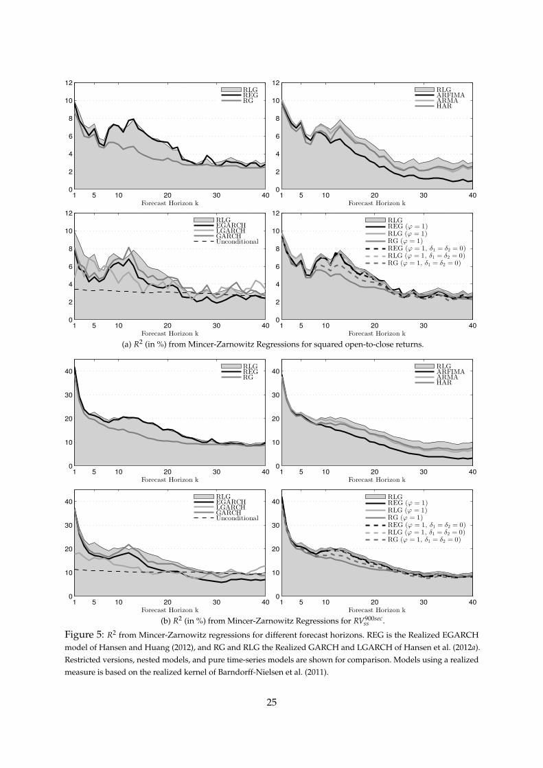
Figure 5a and Figure 5b present performance results for volatility forecasting in the Realized

GARCH framework using Mincer-Zarnowitz type regressions for evaluation purposes. Regres-

sion R2 are shown for each k. We take as dependent variable two volatility proxies namely the

daily open-to-close return squared (5a) and the sub-sampled 15-minute realized variance (5b).

As the independent variable we take the forecast for each k from the range of models presented

above. All models that are based on a realized measure of volatility uses the realized kernel.

For non-linear specifications we set S = 10.000 in the simulation. We take 1126 days as the

estimation window leaving 840 observations for evalution in a rolling-window setup. Such that

the first in-sample window is 2 January 2006 to 30 June 2010 constructing forecasts from 1 July

2010 to 24 August 2010. Rolling the estimation window day by day we create forecasts for the

period 1 July 2010 to 25 October 2013. 39 forecasts for each k are discarded in order to base the

Mincer-Zarnowitz regression on the same number of observations and using the same realized

values.

24

1 5 10 20 30 400

2

4

6

8

10

12

Forecast Horizon k

RLGREGRG

1 5 10 20 30 400

2

4

6

8

10

12

Forecast Horizon k

RLGARFIMAARMAHAR

1 5 10 20 30 400

2

4

6

8

10

12

Forecast Horizon k

RLGEGARCHLGARCHGARCHUnconditional

1 5 10 20 30 400

2

4

6

8

10

12

Forecast Horizon k

RLG

REG (ϕ = 1)

RLG (ϕ = 1)

RG (ϕ = 1)

REG (ϕ = 1, δ1 = δ2 = 0)

RLG (ϕ = 1, δ1 = δ2 = 0)

RG (ϕ = 1, δ1 = δ2 = 0)

(a) R2 (in %) from Mincer-Zarnowitz Regressions for squared open-to-close returns.

1 5 10 20 30 400

10

20

30

40

Forecast Horizon k

RLGREGRG

1 5 10 20 30 400

10

20

30

40

Forecast Horizon k

RLGARFIMAARMAHAR

1 5 10 20 30 400

10

20

30

40

Forecast Horizon k

RLGEGARCHLGARCHGARCHUnconditional

1 5 10 20 30 400

10

20

30

40

Forecast Horizon k

RLG

REG (ϕ = 1)

RLG (ϕ = 1)

RG (ϕ = 1)

REG (ϕ = 1, δ1 = δ2 = 0)

RLG (ϕ = 1, δ1 = δ2 = 0)

RG (ϕ = 1, δ1 = δ2 = 0)

(b) R2 (in %) from Mincer-Zarnowitz Regressions for RV900secss .

Figure 5: R2 from Mincer-Zarnowitz regressions for different forecast horizons. REG is the Realized EGARCHmodel of Hansen and Huang (2012), and RG and RLG the Realized GARCH and LGARCH of Hansen et al. (2012a).Restricted versions, nested models, and pure time-series models are shown for comparison. Models using a realizedmeasure is based on the realized kernel of Barndorff-Nielsen et al. (2011).

25

The top left hand corner of all panels shows the non-restricted versions of RG, RLG, and REG.

The area beneath RLG is filled and added to all other panels for comparison.28 The top right hand

corner shows the pure time series models that work on a realized measure directly, the bottom

left hand corner the nested models, and the bottom right hand corner the restricted models. A

few interesting observations can be made. R2 for REG and RLG are very close and larger for

most k in both panels compared to R2 for all other models. Measured by the R2 both REG and

RLG dominates RG. For the time-series models, the Mincer-Zarnowitz regressions suggest that

the ability of RLG to capture the dynamics of the volatility proxy is slightly better than that of

the time-series models. This, and the fact the ARMA model is among the best performing of the

three for all k, reduce the suspicion of long-memory importance for volatility forecasting. On the

basis of the Mincer-Zarnowitz regressions, we conclude that REG can compete with the pure

time series models. Among the nested models, performance is mixed and dependent on proxy

and evaluation. R2 is volatile for the nested models, but suggest that performance is worse than

RLG for k . 25. For k & 25 the performance of all models converge to the performance of a

model based on the unconditional variance. Among the restricted models, the restriction ϕ = 1

is not important for RG and RLG, but reduce the performance of REG. Removing the leverage

term in the measurement equation slightly improves the performance of RG for a mid-range of

k, and the performance of RLG with and without restrictions are similar.

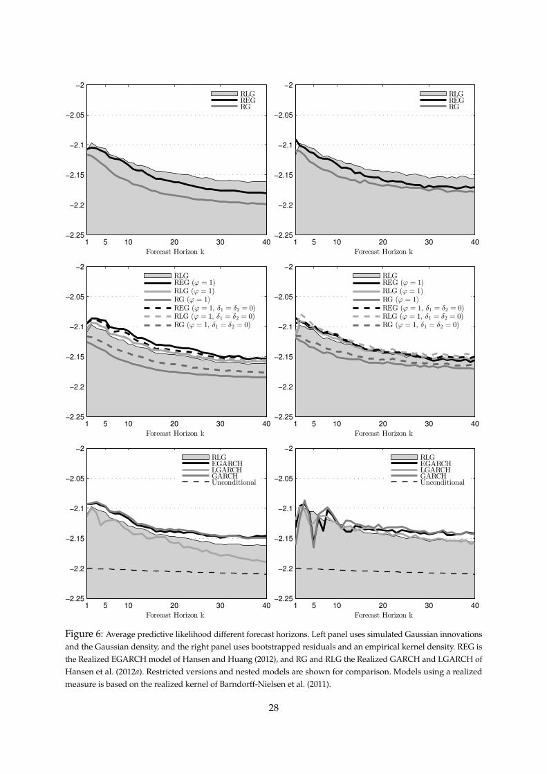
6.2 Density Forecasting

The Realized GARCH framework has much more flexibility to provide also forecasts of the full

density to which we will now turn our attention. Thus, let fM,k (�|Ft, θ) be the k-period ahead

predictive return density of model M, given Ft and θ. For the simulation based approach, we

assume that both zt and ut are conditionally Gaussian and rely on conditional analytic results

(“Rao-Blackwellization”) to obtain the conditional return density. Alas, the return density at t+ k

is Gaussian with mean µ and variance ht+k. For the bootstrap based approach, we utilize that

we have fully specified the law of motion for daily returns and the realized volatility measure.

We simulate the model out k periods S times using the bootstraps for ht+k and a apply a kernel

density estimator to the simulated returns.29 A popular approach to assess the accuracy of a

model’s density forecasts is the predictive likelihood (see Amisano and Giacomini (2007)). This

approach evaluates the model’s density forecast at the realized return. Intuitively, models that

fit the data better give higher density forecasts. Inspired by Maheu and McCurdy (2011) we use

the average predictive likelihood

DM,k =1

T − τ − kmax + 1

T−k

∑t=τ+kmax−k

log fM,k (rt+k|Ft, θ) , k ≥ 1,

28Thus, a model is preferred over RLG if it is above (below) the filled area for the top (bottom) panels for a given k.29We use the in-build MATLAB function ksdensity with a normal kernel with the theoretical optimal bandwith.

26

which we denote DSimM,k and DBoot

M,k for the simulation and bootstrap based approach, respectively.

Statistically, we can compare the ability to forecast return densities for many models in the

Model Confidence Set (MCS) of Hansen et al. (2011). This is done for every choice of k, where we

also use the time series of log fM,k (rt+k|Ft, θ) for t = τ + kmax, . . . , T − k as the loss function for

all M. The MCS is by construction able to account for the variance of the selected loss function,

which is attractive for the bootstrap approach in particular, which is prone to large losses.

6.2.1 Empirical Results

Figure 6 shows DSimM,k and DBoot

M,k in the left and right panel, respectively. For both, we take first for

the initial estimation the in-sample period to be 2 January 2006 to 30 June 2010 (i.e. τ = 1107).30

Second, using the obtained parameter estimates, we set S = 10, 000 and kmax = 40, and determine

log fM,k (rt+k|Ft, θ) for t = τ + kmax using the simulation and bootstrap based approach for all

models. Third, we roll the estimation window one day forward and repeat the two steps. Several

interesting remarks can be made to Figure 6. First, REG and RLG is superior to RG, and RLG

performs better than REG except for k = 1. With parameter restrictions, RLG and REG is close

to be on par. ϕ = 1 is important for all models, but gains from further imposing simplifying

restrictions are observed only for RG. An important message is the good performance of the

nested EG and an ordinary GARCH. LG performs worse. Overall, we conclude that evidence in

favour of using realized volatility measures for the purpose of forecasting the return density of

NOMXC forwards is weak.

To more formally compare the forecast performance of the models we apply the MCS of

Hansen et al. (2011) in Table 9. The objective of the MCS procedure is to determine the set of

“best” models, M?, from a collection of models M0, where “best” here is defined by a loss

function. Thus, one can view the MCS as a set of models that includes the “best” models with a

given level of confidence. With informative data the MCS will consist only of the best model, and

less informative data may result in a MCS with several models. We refer to Hansen et al. (2011)

for details. Overall, the MCS results confirm the visual inspection of the average from Figure 6.

For the unrestricted models, RLG is in M?90% except for k = 1 using bootstrapped innovations.

REG is in M?90% only for small k, and RG is clearly outperformed. Imposing restrictions is

beneficial for RLG and REG as evident from Panel B. From Panel C it is clear that dynamic

modeling of the variance is important for forecasting the return distribution. However, the

added gains from using high-frequency data is small as the nested EGARCH-type model and

the standard GARCH are consistently in M?90%.

30Recall, that we for this part use close-to-close returns. The deterministic roll-over returns are removed andshould be analyzed on their own.

27

1 5 10 20 30 40−2.25

−2.2

−2.15

−2.1

−2.05

−2

Forecast Horizon k

RLG

REGRG

1 5 10 20 30 40−2.25

−2.2

−2.15

−2.1

−2.05

−2

Forecast Horizon k

RLG

REGRG

1 5 10 20 30 40−2.25

−2.2

−2.15

−2.1

−2.05

−2

Forecast Horizon k

RLG

REG (ϕ = 1)

RLG (ϕ = 1)

RG (ϕ = 1)

REG (ϕ = 1, δ1 = δ2 = 0)

RLG (ϕ = 1, δ1 = δ2 = 0)

RG (ϕ = 1, δ1 = δ2 = 0)

1 5 10 20 30 40−2.25

−2.2

−2.15

−2.1

−2.05

−2

Forecast Horizon k

RLG

REG (ϕ = 1)

RLG (ϕ = 1)

RG (ϕ = 1)

REG (ϕ = 1, δ1 = δ2 = 0)

RLG (ϕ = 1, δ1 = δ2 = 0)

RG (ϕ = 1, δ1 = δ2 = 0)

1 5 10 20 30 40−2.25

−2.2

−2.15

−2.1

−2.05

−2

Forecast Horizon k

RLGEGARCHLGARCHGARCHUnconditional

1 5 10 20 30 40−2.25

−2.2

−2.15

−2.1

−2.05

−2

Forecast Horizon k

RLGEGARCHLGARCHGARCHUnconditional

Figure 6: Average predictive likelihood different forecast horizons. Left panel uses simulated Gaussian innovationsand the Gaussian density, and the right panel uses bootstrapped residuals and an empirical kernel density. REG isthe Realized EGARCH model of Hansen and Huang (2012), and RG and RLG the Realized GARCH and LGARCH ofHansen et al. (2012a). Restricted versions and nested models are shown for comparison. Models using a realizedmeasure is based on the realized kernel of Barndorff-Nielsen et al. (2011).

28

Tabl

e9:

MC

Sre

sult

sfo

rD

Sim

M,k

(lef

t)an

dD

Boo

tM

,k(r

ight

).

k1

25

1020

3040

12

510

2030

40Pa

nelA

:Unr

estr

icte

dM

odel

s

RLG

0.86

?1.

00?

1.00

?1.

00?

1.00

?1.

00?

1.00

?0.

091.

00?

1.00

?1.

00?

1.00

?1.

00?

1.00

?

RE

G1.

00?

0.41

?0.

38?

0.57

?0.

000.

000.

001.

00?

0.62

?0.

11?

0.22

?0.

000.

000.

00R

G0.

70?

0.00

0.00

0.00

0.00

0.00

0.00

0.09

0.16

?0.

000.

000.

000.

000.

00

Pane

lB:R

estr

icte

dM

odel

s

RLG

0.05

0.22

?0.

020.

020.

070.

010.

000.

080.

000.

040.

010.

28?

0.14

?0.

00R

EG(ϕ

=1)

1.00

?1.

00?

1.00

?1.

00?

1.00

?1.

00?

0.84

?0.

12?

0.02

0.33

?0.

71?

0.73

?0.

65?

0.03

RLG

(ϕ=

1)0.

16?

0.33

?0.

050.

030.

21?

0.07

0.00

0.08

0.00

0.49

?0.

010.

28?

0.65

?0.

00R

G(ϕ

=1)

0.00

0.00

0.00

0.00

0.00

0.00

0.00

0.08

0.00

0.00

0.01

0.14

?0.

060.

00R

EG(ϕ

=1,

δ 1=

δ 2=

0)0.

99?

0.36

?0.

29?

0.28

?0.

25?

0.56

?1.

00?

1.00

?0.

001.

00?

1.00

?0.

73?

0.65

?0.

03R

LG(ϕ

=1,

δ 1=

δ 2=

0)0.

16?

0.33

?0.

050.

030.

25?

0.56

?0.

66?

0.08

1.00

?0.

77?

0.95

?1.

00?

1.00

?1.

00?

RG(ϕ

=1,

δ 1=

δ 2=

0)0.

16?

0.04

0.01

0.01

0.03

0.01

0.00

0.08

0.00

0.03

0.01

0.28

?0.

14?

0.00

Pane

lC:A

llM

odel

sin

cl.B

ench

mar

ks

RLG

0.12

?0.

43?

0.06

0.02

0.08

0.02

0.00

0.13

?0.

000.

040.

010.

40?

0.21

?0.

00R

EG

0.30

?0.

43?

0.06

0.02

0.00

0.00

0.00

0.64

?0.

000.

020.

010.

000.

000.

00R

G0.

12?

0.02

0.00

0.00

0.00

0.00

0.00

0.14

?0.

000.

010.

000.

000.

000.

00R

EG(ϕ

=1)

0.99

?1.

00?

1.00

?1.

00?

1.00

?0.

90?

0.66

?0.

22?

0.02

0.33

?0.

86?

0.72

?0.

28?

0.07

RLG

(ϕ=

1)0.

30?

0.56

?0.

090.

040.

28?

0.10

?0.

000.

14?

0.00

0.49

?0.

020.

49?

0.28

?0.

00R

G(ϕ

=1)

0.00

0.00

0.00

0.00

0.00

0.00

0.00

0.10

0.00

0.00

0.01

0.21

?0.

080.

00R

EG(ϕ

=1,

δ 1=

δ 2=

0)0.

99?

0.78

?0.

67?

0.62

?0.

48?

0.42

?0.

66?

1.00

?0.

001.

00?

1.00

?0.

72?

0.21

?0.

07R

LG(ϕ

=1,

δ 1=

δ 2=

0)0.

30?

0.56

?0.

090.

040.

38?

0.56

?0.

66?

0.14

?1.

00?

0.76

?0.

95?

0.72

?0.

28?

0.89

?

RG(ϕ

=1,

δ 1=

δ 2=

0)0.

12?

0.08

0.03

0.02

0.04

0.01

0.00

0.13

?0.

000.

020.

010.

40?

0.21

?0.

00E

GA

RC

H1.

00?

0.78

?0.

67?

0.62

?0.

65?

0.90

?1.

00?

0.13

?0.

000.

010.

020.

72?

0.57

?1.

00?

LGA

RC

H0.

30?

0.56

?0.

060.

020.

040.

000.

000.

13?

0.00

0.02

0.02

0.72

?0.

26?

0.00

GA

RC

H0.

99?

0.78

?0.

67?

0.62

?0.

75?

1.00

?0.

66?

0.10

0.00

0.02

0.86

?1.

00?

1.00

?0.

89?

MC

Sp-

valu

esfo

rth

epr

edic

tive

likel

ihoo

dfo

rd

iffe

rent

fore

cast

hori

zons

,k.T

hefo

reca

sts

inM∗ 90

%ar

eid

enti

fied

byan

aste

risk

.Lef

tpan

elu

ses

sim

ula

ted

Gau

ssia

nin

nova

tion

san

dth

eG

auss

ian

dens

ity,

and

the

righ

tpan

elus

esbo

otst

rapp

edre

sidu

als

and

anem

piri

calk

erne

lden

sity

.REG

isth

eR

ealiz

edEG

AR

CH

mod

elof

Han

sen

and

Hu

ang

(201

2),a

ndR

Gan

dR

LG

the

Rea

lized

GA

RC

Han

dL

GA

RC

Hof

Han

sen

etal

.(20

12a)

.Res

tric

ted

vers

ions

and

nest

edm

odel

sar

esh

own

for

com

par

ison

.M

odel

sus

ing

are

aliz

edm

easu

reis

base

don

the

real

ized

kern

elof

Barn

dorf

f-N

iels

enet

al.(

2011

).

29

7 Conclusion

We have explored the transaction records from NOMXC from January 2006 to October 2013 and

discussed the construction of continual nearby contracts. We have estimated a range of realized

measures of volatility that have been developed mostly for stock markets, and documented

an inherent bias for the underlying volatility when applied to NOMXC forwards. This bias is

important to take into careful consideration when using realized measures to study NOMXC

forwards, and it opens an interesting area to further explore as realized measures of volatility

must be adjusted to this market. We use a selection of “traditional” realized measures of volatility

to enrich the information set of GARCH models in the Realized GARCH framework of Hansen

et al. (2012a). Within this framework, we were able to validate possible gains from utilizing

realized measures of volatility, despite their bias, for the modeling and forecasting of the con-

ditional return variance. Estimations revealed a gain from utilizing data at higher frequencies

by comparing to ordinary EGARCH models, which is nested in the Realized EGARCH model

considered. Improved empirical fit was obtained in-sample as measured by the log-likelihood

and the obtained results illustrated the importance of careful volatility estimation as the level is

time-dependent but predictable. However, the out-of-sample assessment was less in favor of us-

ing realized measures. The added value was limited considering both regular and bootstrapped

rolling-window forecasts for volatility and return density forecasting. Overall, the Realized

GARCH framework was found to provide slightly better volatility forecasts than standard daily

models, which conversely in some cases provided better density forecasts. It is expected that

these results can be significantly improved with a better understanding of how to use realized

measures of volatility in this market. This is an important area to study going forward. Another

appealing extension is in the multivariate setting, where co-volatilities between the different

NOMXC forwards, and between the forwards and other energy markets such as coal, gas, and

oil, are important to many (e.g. energy and utility companies). This could for example extend

the daily analysis in Bauwens et al. (2012) to incorporate intraday data. Another interesting

venue would be to adapt the Hansen et al. (2012b) approach to the energy markets.

30

References

Amisano, G. and Giacomini, R. (2007), ‘Comparing Density Forecasts via Weighted Likelihood

Ratio Tests’, Journal of Business & Economic Statistics 25, 177–190.

Andersen, T. G., Bollerslev, T. and Diebold, F. X. (2009), Parametric and nonparametric volatility

measurement, in L. P. Hansen and Y. Ait-Sahalia, eds, ‘Handbook of Financial Econometrics’,

North-Holland, Amsterdam.

Barndorff-Nielsen, O. E., Hansen, P. R., Lunde, A. and Shephard, N. (2009), ‘Realised kernels in

practice: Trades and quotes’, Econometrics Journal 12, C1–C32.

Barndorff-Nielsen, O. E., Hansen, P. R., Lunde, A. and Shephard, N. (2011), ‘Multivariate realised

kernels: consistent positive semi-definite estimators of the covariation of equity prices with

noise and non-synchronous trading’, Journal of Econometrics 162, 149–169.

Barndorff-Nielsen, O. E. and Shephard, N. (2002), ‘Econometric analysis of realised volatility

and its use in estimating stochastic volatility models’, Journal of the Royal Statistical Society B

64, 253–280.

Barndorff-Nielsen, O. E. and Shephard, N. (2004), ‘Power and bipower variation with stochastic

volatility and jumps (with discussion)’, Journal of Financial Econometrics 2, 1–37.

Barndorff-Nielsen, O. E. and Shephard, N. (2007), Variation, jumps and high frequency data

in financial econometrics, in R. Blundell, T. Persson and W. K. Newey, eds, ‘Advances in

Economics and Econometrics. Theory and Applications, Ninth World Congress’, Econometric

Society Monographs, Cambridge University Press, pp. 328–372.

Bauwens, L., Hafner, C. M. and Pierret, D. (2012), ‘Multivariate volatility modeling of electricity

futures’, Journal of Applied Econometrics, forthcoming .

Benth, F. E., Álvaro Cartea and Kiesel, R. (2008a), ‘Pricing forward contracts in power markets by

the certainty equivalence principle: Explaining the sign of the market risk premium’, Journal

of Banking & Finance 32(10), 2006 – 2021.

Benth, F. E., Benth, J. S. and Koekebakker, S. (2008b), Stochastic Modelling of Electricity and Related

Markets, World Scientific Publishing, Toh Tuck Link, Singapore.

Benth, F. E. and Koekebakker, S. (2008), ‘Stochastic modeling of financial electricity contracts’,

Energy Economics 30(3), 1116 – 1157.

Boudt, K., Croux, C. and Laurent, S. (2011), ‘Outlyingness Weighted Covariation’, Journal of

Financial Econometrics 9(4), 657–684.

31

Corsi, F. (2009), ‘A simple approximate long-memory model of realized volatility’, Journal of

Financial Econometrics .

Deaton, A. and Laroque, G. (1992), ‘On the behavior of commodity prices’, Rev. Financ. Econ.

Stud. 59, 1–23.

Doornik, J. and Ooms, M. (2014), ‘A package for estimating, forecasting and simulating arfima

models: Arfima package 1.07 for ox’.

Engle, R. F. (2002), ‘New frontiers for ARCH models’, Journal of Applied Econometrics 17, 425–446.

Escribano, A., Pena, J. I. and Villaplana, P. (2011), ‘Modelling electricity prices: International

evidence’, Oxford Bulletin of Economics and Statistics 73, 622–650.

Geman, H. and Roncoroni, A. (2006), ‘Understanding the fine structure of electricity prices’,

Journal of Business 79, 1225–1261.

Hansen, P. R. and Huang, Z. (2012), ‘Exponential garch modeling with realized measures of

volatility’, Working Paper, CREATES .

Hansen, P. R., Huang, Z. and Shek, H. H. (2012a), ‘Realized garch: A joint model of returns and

realized measures of volatility’, Journal of Applied Econometrics 27, 877–906.

Hansen, P. R. and Lunde, A. (2005), ‘A realized variance for the whole day based on intermittent

high-frequency data’, Journal of Financial Econometrics 3, 525–544.

Hansen, P. R. and Lunde, A. (2006), ‘Realized variance and market microstructure noise’, Journal

of Business and Economic Statistics 24, 127–218. The 2005 Invited Address with Comments and

Rejoinder.

Hansen, P. R. and Lunde, A. (2011), Forecasting volatility using high-frequency data, in

M. Clements and D. Hendry, eds, ‘The Oxford Handbook of Economic Forecasting’, Ox-

ford: Blackwell, chapter 19, pp. 525–556.

Hansen, P. R., Lunde, A. and Nason, J. M. (2011), ‘The model confidence set’, Econometrica

79, 456–497.

Hansen, P. R., Lunde, A. and Voev, V. (2012b), ‘Realized beta garch: A multivariate garch model

with realized measures of volatility and covolatility’, Working Paper, CREATES .

Hansen, P. R., Lunde, A. and Voev, V. (2014), ‘Realized beta garch: A multivariate garch model

with realized measures of volatility’, Journal of Aplied Econometrics .

Haugom, E. (2011), ‘Some stylized facts about high-frequency nord pool forward prices’, The

Journal of Energy Markets 4.

32

Haugom, E. (2013), ‘Predicting realized volatility for nord pool forward prices by including

volatility spillover and covariance effects’, The Journal of Energy Markets 6.

Haugom, E., Westgaard, S., Solibakke, P. B. and Lien, G. (2011a), ‘Modelling day-ahead nord

pool forward-price volatility: Realized volatility versus garch models’, International Research

Journal of Finance and Economics .

Haugom, E., Westgaard, S., Solibakke, P. B. and Lien, G. (2011b), ‘Realized volatility and the

influence of market measures on predictability: Analysis of Nord Pool forward electricity

data’, Energy Economics 33, 1206 – 1215.

Haugom, E., Westgaard, S., Solibakke, P. B. and Lien, G. (2012), ‘Covariance estimation using

high-frequency data: An analysis of nord pool electricity forward data’, Journal of Energy and

Power Engineering .

Higgs, H. and Worthington, A. (2008), ‘Stochastic price modeling of high volatility, mean-

reverting, spike-prone commodities: The australian wholesale spot electricity market’, Energy

Economics 30(6), 3172 – 3185. Technological Change and the Environment.

Maheu, J. M. and McCurdy, T. H. (2011), ‘Do high-frequency measures of volatility improve

forecasts of return distributions?’, Journal of Econometrics 160(1), 69–76.

Malo, P. and Kanto, A. (2006), ‘Evaluating multivariate garch models in the nordic electricity

markets’, Communications in Statistics - Simulation and Computation 35(1), 117–148.

NASDAQ OMX Commodities (2011a), Productcalendar.

NASDAQ OMX Commodities (2011b), Trade at NASDAQ OMX Commodities Europe’s Financial

Market.

NASDAQ OMX Commodities (2011c), Trading and Clearing Financial Power Contracts.

Pen, Y. L. and Sévi, B. (2010), ‘Volatility transmission and volatility impulse response functions

in european electricity forward markets’, Energy Economics 32(4), 758 – 770. Policymaking

Benefits and Limitations from Using Financial Methods and Modelling in Electricity Markets.

Protter, P. (2005), Stochastic Integration and Differential Equations, New York: Springer-Verlag.

Veraart, A. E. D. and Veraart, L. A. M. (2013), Modelling electricity day-ahead prices by multi-

variate levy semistationary processes, in Benth, Kholodnyi and Laurence, eds, ‘Forthcoming

in Quantitative Energy Finance’, Springer, Berlin.

Zhang, L., Mykland, P. A. and Aït-Sahalia, Y. (2005), ‘A tale of two time scales: Determining inte-

grated volatility with noisy high frequency data’, Journal of the American Statistical Association

100, 1394–1411.

33

Research Papers 2013

2013-02: Almut E. D. Veraart and Luitgard A. M. Veraart: Risk premia in energy markets

2013-03: Stefano Grassi and Paolo Santucci de Magistris: It’s all about volatility (of volatility): evidence from a two-factor stochastic volatility model

2013-04: Tom Engsted and Thomas Q. Pedersen: Housing market volatility in the OECD area: Evidence from VAR based return decompositions

2013-05: Søren Johansen and Bent Nielsen: Asymptotic analysis of the Forward Search

2013-06: Debopam Bhattacharya, Pascaline Dupasand Shin Kanaya: Estimating the Impact of Means-tested Subsidies under Treatment Externalities with Application to Anti-Malarial Bednets

2013-07: Sílvia Gonçalves, Ulrich Hounyo and Nour Meddahi: Bootstrap inference for pre-averaged realized volatility based on non-overlapping returns

2013-08: Katarzyna Lasak and Carlos Velasco: Fractional cointegration rank estimation

2013-09: Roberto Casarin, Stefano Grassi, Francesco Ravazzolo and Herman K. van Dijk: Parallel Sequential Monte Carlo for Efficient Density Combination: The Deco Matlab Toolbox

2013-10: Hendrik Kaufmann and Robinson Kruse: Bias-corrected estimation in potentially mildly explosive autoregressive models

2013-11: Robinson Kruse, Daniel Ventosa-Santaulària and Antonio E. Noriega: Changes in persistence, spurious regressions and the Fisher hypothesis

2013-12: Martin M. Andreasen, Jesús Fernández-Villaverde and Juan F. Rubio-Ramírez: The Pruned State-Space System for Non-Linear DSGE Models: Theory and Empirical Applications

2013-13: Tom Engsted, Stig V. Møller and Magnus Sander: Bond return predictability in expansions and recessions

2013-14: Charlotte Christiansen, Jonas Nygaard Eriksen and Stig V. Møller: Forecasting US Recessions: The Role of Sentiments

2013-15: Ole E. Barndorff-Nielsen, Mikko S. Pakkanen and Jürgen Schmiegel: Assessing Relative Volatility/Intermittency/Energy Dissipation

2013-16: Peter Exterkate, Patrick J.F. Groenen, Christiaan Heij and Dick van Dijk: Nonlinear Forecasting With Many Predictors Using Kernel Ridge Regression

2013-17: Daniela Osterrieder: Interest Rates with Long Memory: A Generalized Affine Term-Structure Model

2013-18: Kirstin Hubrich and Timo Teräsvirta: Thresholds and Smooth Transitions in Vector Autoregressive Models

2013-19: Asger Lunde and Kasper V. Olesen: Modeling and Forecasting the Distribution of Energy Forward Returns - Evidence from the Nordic Power Exchange