Modeling elves observed by FORMOSAT-2 satellite

Modeling elves observed by FORMOSAT-2 satellite

Cheng-Ling Kuo,1,2 A. B. Chen,1 Y. J. Lee,1 L. Y. Tsai,1 R. K. Chou,1 R. R. Hsu,1

H. T. Su,1 L. C. Lee,2 S. A. Cummer,3 H. U. Frey,4 S. B. Mende,4 Y. Takahashi,5

and H. Fukunishi5

Received 18 March 2007; revised 20 July 2007; accepted 31 July 2007; published 22 November 2007.

[1] The ISUAL experiment on the FORMOSAT-2 satellite has confirmed the existence ofionization and Lyman-Birge-Hopfield (LBH) band emissions in elves. In this paper,an in-depth study of the ISUAL recorded elves was carried out. Numerical simulationresults of elves based on an electromagnetic finite difference time domain (FDTD) modelof the emissions between 185–800 nm and of their spatial-temporal evolution arepresented. To account for the effect of atmospheric attenuation, three major attenuationmechanisms: O2, O3, and molecular Rayleigh scattering are considered. Validations of theelectromagnetic FDTD model were conducted in three ways: by comparing the calculatedand observed photon fluxes in the ISUAL spectrophotometric channels, by directlycomparing the simulated and observed morphologies of elves, and by comparing thecomputed photon counts of the ISUAL Imager based on the derived peak currents for twoelve-associated NLDN (National Lightning Detection Network) cloud-to-grounddischarges (CGs) with those recorded by the ISUAL Imager. In all three ways,very good agreement was achieved.

Citation: Kuo, C.-L., et al. (2007), Modeling elves observed by FORMOSAT-2 satellite, J. Geophys. Res., 112, A11312, doi:10.1029/

2007JA012407.

1. Introduction

[2] Thunderstorm-related optical flashes in the lowerionosphere and middle atmosphere are categorized intoseveral types of transient luminous events (TLEs), includingsprites [Franz et al., 1990; Sentman et al., 1995; Pasko etal., 1997; Su et al., 2002], elves [Inan et al., 1991; Boeck etal., 1992; Fukunishi et al., 1996], blue jets and gigantic jets[Wescott et al., 1995; Pasko et al., 2002; Su et al., 2003].Elves were first discovered in the space shuttle images[Boeck et al., 1992] and were subsequently identifiedfrom ground observations using high-speed photometry[Fukunishi et al., 1996]. The cause of elves is believed tobe heating of the electrons by the electromagnetic pulses(EMPs) emitted from cloud-to-ground discharges [Inan etal., 1996; Fernsler and Rowland, 1996; Barrington-Leighand Inan, 1999; Veronis et al., 1999]. The E field drivenelectrons collide with molecular nitrogen and molecularoxygen, inducing excitation and/or ionization and eventu-ally resulting in the expanding luminous emissions in the

lower ionosphere. The typical altitude of elves is in therange of 80–95 km and their lateral dimension is 200–500 km. The short luminous duration (�1 ms) and thesevere atmospheric attenuation of short-wavelength emis-sions have limited the success in obtaining the full spectro-scopic information of elves from ground observations. Forexample, several high-speed (�60 kHz) photomultiplier-based photometric measurements of elves [Inan et al., 1997;Barrington-Leigh and Inan, 1999] have been performed,but the full band emissions of elves, especially in the UVand FUV bands, have not been resolved.[3] Recently, the ISUAL experiment on FORMOSAT-2

satellite has confirmed the existence of ionization andLyman-Birge-Hopfield (LBH) band emissions in elves[Mende et al., 2005]. This exciting result demonstratedthe advantage of space-borne observation platform. Herewe report in-depth numerical simulations based on anelectromagnetic finite difference time domain (FDTD)model to elucidate the observed characteristics of theISUAL elves. An electromagnetic FDTD model has beenused to in the past to explain the morphologies and topredict the photometric behavior of ground-observed elves[Inan et al., 1997; Pasko et al., 1998; Barrington-Leigh andInan, 1999; Veronis et al., 1999]. In this paper, a similarelectromagnetic FDTD model was employed to predict theelves emissions between 185–800 nm, to project thespatial-temporal evolution, to explain the morphology andto elucidate the photometric behavior of the ISUALrecorded elves. The numerical study includes an electriccurrent which flows in the conducting channel of a cloud-to-

JOURNAL OF GEOPHYSICAL RESEARCH, VOL. 112, A11312, doi:10.1029/2007JA012407, 2007ClickHere

for

FullArticle

1Department of Physics, National Cheng Kung University, Tainan,Taiwan.

2Institute of Space Science, National Central University, Jhongli,Taiwan.

3Electrical and Computer Engineering Department, Duke University,Durham, North Carolina, USA.

4Space Sciences Laboratory, University of California, Berkeley,California, USA.

5Department of Geophysics, Tohoku University, Sendai, Japan.

Copyright 2007 by the American Geophysical Union.0148-0227/07/2007JA012407$09.00

A11312 1 of 18

http://dx.doi.org/10.1029/2007JA012407

ground lighting for an extended period. This nearly impul-sive current radiates an electromagnetic dipole field, whosestrength at the lower ionosphere can be computed via theMaxwell equations and a coupled electron density continu-ity equation. The E field–energized electrons impact, ex-cite, or ionize the ambient molecular nitrogen and oxygen,which subsequently emit the observed luminous emissions.

2. ISUAL Experiment

[4] The elves data presented in this paper were recordedby the ISUAL payload on FORMOSAT-2 satellite [Chern etal., 2003]. FORMOSAT-2 is a Sun-synchronous satellitewhich is capable of surveying the whole globe with 14 dailyrevisiting orbits. The ISUAL payload consists of an ICCDImager, a six-channel spectrophotometer (SP) and an arrayphotometer (AP). The Imager data were obtained through a623–750 nm filter with an image frame integration time of14 ms. The key SP data are from channel 2 (centered at337 nm; bandwidth 5.6 nm) and channel 3 (centered at391.4 nm; bandwidth 4.2 nm) of the ISUAL SP. Other SPchannels include SP1 (150–290 nm), SP4 (608.9 –753.4 nm), SP5 (centered at 777.4 nm), and SP6 (228.2–410.2 nm). The sampling rate of the ISUAL SP is 10 kHz.The ISUAL AP contains a blue (370–450 nm) and a red(530–650 nm) band multiple-anode photometers. Eachband of AP has 16 vertically stacked PMTs with a combinedfield-of-view (FOV) of 22 deg (H) � 3.6 deg (V) [Chern etal., 2003; Mende et al., 2005; Kuo et al., 2005]. The ISUALImager, SP and AP are coaligned at the center of theirviews. ISUAL Imager and SP are bore-sighted, and theirFOV is approximately 20 deg (H) � 5 deg (V). Figure 1shows the observational geometry of the ISUAL payloadonboard the FORMOSAT-2. The Imager and SP FOVsproject out an area of nearly two million square kilometerson Earth’s surface (the gray area in Figure 1), with the nearedge at a distance of 2370 km (lateral AB � 910 km), thelimb at 3370 km away (lateral CD � 1210 km) and the far

edge for 90 km altitude at a distance of 4410 km (lateral EF� 1590 km).

3. Model Formulation

3.1. Electromagnetic FDTD Model

[5] The electromagnetic FDTD model simulates theeffects of the electromagnetic pulse (EMP) released by thevertical current of a cloud-to-ground lightning in a circularly

symmetric (@

@f= 0) cylindrical coordinate system (r, f, z),

and involves Maxwell equations that couples with anelectron density continuity equation [Pasko et al., 1998;Veronis et al., 1999]. The spatial-and-temporal-varyinglightning current waveform is assumed to posses the fol-lowing form,

Js r; z; tð Þ ¼ IpT tð ÞS r; zð Þ: ð1Þ

Here, the peak current Ip occurs at t = tr; T(t) is the time-

varying function of the current waveform, and T(t) =t

trat

t < tr or e� t�trð Þ=tf½ �2 at t tr where tr and tf are therisetime and the fall-time of the current. The currentwaveform of the +CGs typically has a risetime of �10 ms[Rakov and Uman, 2003, p. 233], which is longer than thatof the �CGs (�5 ms) [Rakov and Uman, 2003, p. 7]. Therisetimes of the +CG current waveform could be up tohundreds of microseconds for very long upward negativeleaders [Rakov and Uman, 2003, p. 234]. However, such acomplex discharge process is not considered in ourmodeling. The fall-time of the current waveform is inthe order of hundreds of microseconds [Rakov and Uman,2003, p. 215, and references therein]. Therefore for atypical +CG, the risetime tr and the fall-time tf is chosento be 10 ms and 100 ms in our model. Figure 2a shows a+CG with a peak current of 280 kA and b = 0.5, whichgave the best fitted to the ISUAL recorded elve on7 August 2004 1801:22 universal time (UT) and is less thanthe highest directly measured +CG currents of �300 kA[Rakov and Uman, 2003, p. 214, and references therein].The spatial distribution function of the current waveform

satisfies S(r, z) =1

A0

e�r=r20 for z < a or

1

A0

e�r=r20� z�að Þ2=z2

0 for

z a, where A0 is a normalized area constant and A0 =Z 1

0

e�r=r20 2prdr = pr0

2; ro and zo are chosen to be three

times of the cell sizes in the r direction (2 km) andz direction (0.5 km), and a is the current channel lengthwhich is assumed to be 10 km. The current channel length istypically 6 km for �CG and 10 km for +CG. The expecteddisparity between them is in the distance effect, which isless significant for far field (>100 km) since the E field

magnitude decays as E(r) � 1

rat the elves altitude. From our

numerical studies, the maximum E fields at elve altitude87 km were �30 V/m and �27 V/m for a current channellength of 10 km and 6 km, respectively. Also, if the currentrisetime is 5 ms, instead of 10 ms, the E field magnitude froma typical �CG or +CG at the elve altitude would differ byless than 5%. The FDTD model itself is independent of thepolarity of the CGs. Also the E field deviation due to thechanges in the current waveform and channel length is lessthan 10%.

Figure 1. Observational configuration of the ISUALinstruments onboard the FORMOSAT-2 satellite (labeledas ‘‘S’’). The FOVof ISUAL Imager and SP cover a regionof nearly two million square kilometers on Earth’s surface(gray area).

A11312 KUO ET AL.: FORMOSAT-2 SATELLITE RECORDED ELVES

2 of 18

A11312

[6] The assumed Gaussian form of the current channelwidth makes the calculated pulses (E or B field) propagationsmoother and reduces the ringing effect due to the numer-ical dispersion [Taflove and Hagness, 2005, p. 34]. Thelarge sampling grid, 3Dr, of the current pulse decreases theerror in computing the phase velocity [Taflove and Hagness,2005, Figure 2.2, p. 35]. However, these requirements makethe lightning channel unusually broad. For a field point at analtitude of 87 km, the distance between current channelcenter and the field point is j~rj 87 km. At the far-fieldlimit j~rj � j~r0j, the E field magnitude at field point is

proportional to j~r �~r0j�1 � j~rj�1 (1 � ~r 0j j~rj j cosh) where the

distance between the lightning channel center and broadcurrent channel edge j~r0j is about 6 km (3Dr), and h is aangle between ~r and ~r0. The expected error owing to thebroad current channel is minor since j~rj � j~r0j. Thisassessment will be further confirmed in section 4.1, bycomparing the predicted E field from the FDTD model andthat computed by transmission line model (TL) at 100 kmaway.[7] We used the MSIS model [Hedin, 1991] to calculate

molecular nitrogen and molecular oxygen density profilesin our model. The ambient electron density profile is shownin Figure 2b and has the form of ne(z) = 1.43 � 107

exp(�0.15 � h0) exp [(hb � 0.15) � (z � h0)] (cm�3),where hb = 0.5 km�1 at the effective reflection height; z isthe altitude of interest in units of kilometers and h0 is thenighttime VLF reflection height of �85 km [Cummer et al.,1998; Barrington-Leigh et al., 2001]. In Figure 2c, the totalconductivity used in our model can be calculated using stotal= si + se, which contains both the ion (si) and electron (se)components. The ambient ion conductivity profile is adop-

ted from Volland’s [1995] model, si = 1/X3i¼1

Aie�Biz where

Ai

1012Wm;

Bi

km�1

� �= (46.9, 4.527)1, (22.2, 0.375)2, (5.9,

0.121)3, [Volland, 1995, p. 249, and references therein]. Theelectron conductivity is represented by se = qemeNe whereqe is electron charge, Ne is electron density, and me ismobility, which is a function of the reduced E field, E/N,and can be derived from experimental swarm data [Pasko etal., 1997, and references therein]. The electron componentse of the total conductivity is a low-frequency approxima-

tion (wave frequency, w, is much lower than the electroncollision frequency, veff). Arguably, besides depending onthe electron density, conductivity is also a function of the

wave-frequency via s(w) =q2ene

meveff

1

1þ w2=v2eff

� � [Raizer,

1997, p. 44] where me is electron mass. At 87 km altitude,

the collision frequency veff =qe

meme

is 16 MHz for E = Ek,

which is the conventional breakdown threshold field andwill be defined in the text after equation (2), and thecollision frequency is 0.6 MHz for a low field E � 0; thecollision frequencies at this altitude for both E fields aremuch higher than the wave frequency in the VLF range (3–30 kHz). Moreover, electromagnetic pulses with E fieldstrength exceeding 0.3 times of the conventional breakdownthreshold field at this altitude is sufficient to induce the firstpositive band nitrogen emissions of elves [Veronis et al.,1999]. Therefore treating the conductivity as a low-frequen-cy approximation will have minor effect on our emission

calculation, thus s(w) � q2ene

meveff= qemene is used in conduc-

tivity term of Maxwell equations. The electron densitycontinuity equation is

dne

dt¼ vi � vað Þne; ð2Þ

where ne, vi and va are the electron density, the ionizationrate and dissociative attachment (O2 + e� ! O� + O) rate,respectively. The values of vi and va are related to thestrength of the E field which will be derived from Maxwellequations. The conventional breakdown threshold field isdefined as the E field that produces vi = va [Raizer, 1997,pp. 135–136; Liu et al., 2006]. In return, the change inelectron density will modify the ambient conductivity andalter the strength of the E field. The three-body attachmentprocess (A + O2 + e� ! A + O2

�), where A is molecularoxygen or molecular nitrogen in the lower-ionosphere Dregion, has a timescale >1 s and is not included, since themodel deals with processes that last only for a fewmilliseconds [Glukhov et al., 1992; Pasko et al., 1997].[8] The numerical simulation domain extends from z =

0 km to z = 100 km and r = 600 km. For EM waves in theVLF range (3–30 kHz), where the lightning radiated

Figure 2. (a) Current waveform (peak current 280 kA, risetime tr = 10 ms, and fall-time tf = 100 ms) foran assumed CG lightning in our electromagnetic FDTD model, (b) assumed profiles of the neutral speciesdensity, electron density in the upper atmosphere, and (c) the total conductivity including both ionic andelectronic contributions.


3 of 18

A11312

electromagnetic field is most intense, the ground and theboundary at 100 km altitude can be assumed to be perfectlyconducting [Inan et al., 1996]. For the boundary at 100 km,a previous study has shown that only negligible EM waveenergy can penetrate into the lower ionosphere above 95 kmaltitude [Taranenko et al., 1993]. For a vertical lightningcurrent above a perfectly conductive ground, only thevertical component of the radiated E field is observed at afar-field point on the ground. For an imperfectly conductiveground, the image current below the ground is not strictlyequal to the magnitude of lightning current above it. Thehorizontal component of the E field contributed by the realand the image currents does not cancel. However, in ourmodel, we assume the ground to be perfectly conductiveand the tilting effect of lightning current has not beenconsidered [Rakov and Uman, 2003, p.162, and referencestherein].

3.2. Optical Emission Models

[9] We use the ELENDIF code [Morgan and Penetrante,1990] and the cross section data of N2(B

3Pg), N2(C3Pu),

N2(B03Su

�), N2(a1Pg) [Cartwright et al., 1977], N2

+(A2Su+)

[Cartwright et al., 1975] and N2+(B2Su

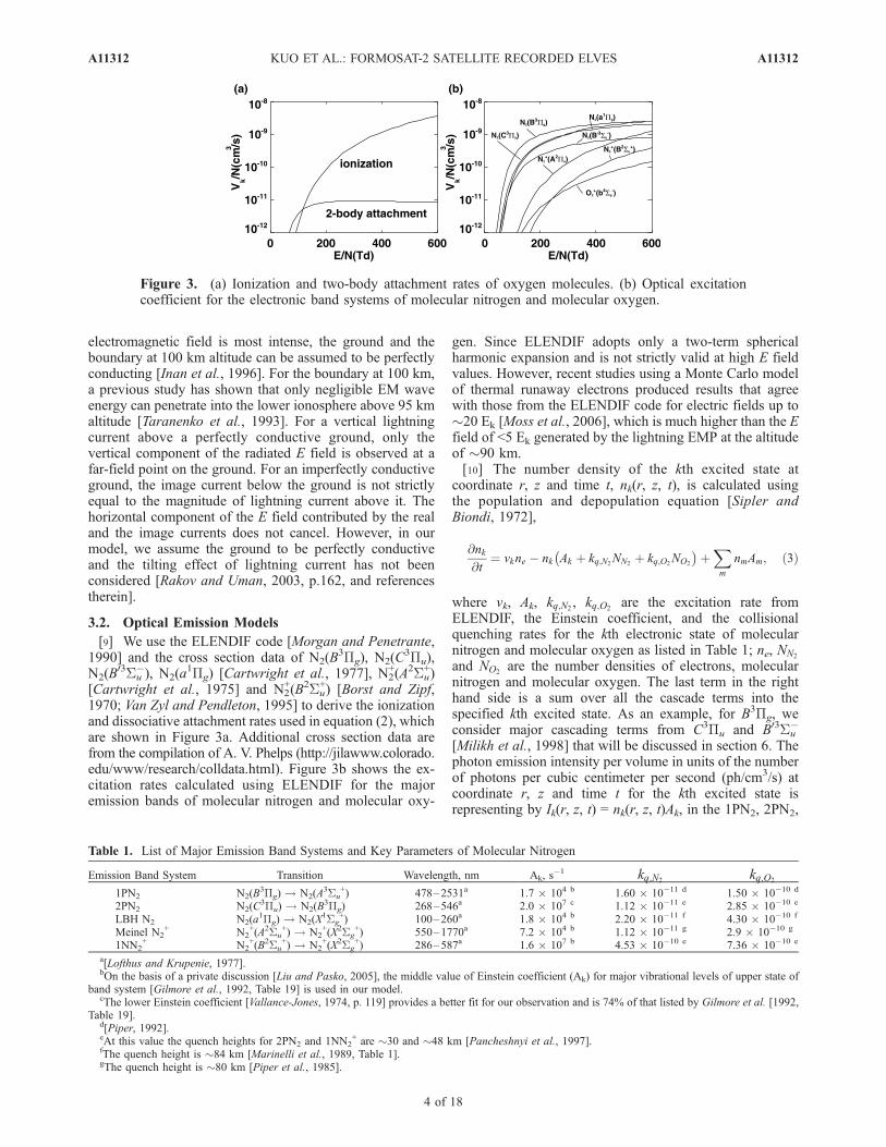
+) [Borst and Zipf,1970; Van Zyl and Pendleton, 1995] to derive the ionizationand dissociative attachment rates used in equation (2), whichare shown in Figure 3a. Additional cross section data arefrom the compilation of A. V. Phelps (http://jilawww.colorado.edu/www/research/colldata.html). Figure 3b shows the ex-citation rates calculated using ELENDIF for the majoremission bands of molecular nitrogen and molecular oxy-

gen. Since ELENDIF adopts only a two-term sphericalharmonic expansion and is not strictly valid at high E fieldvalues. However, recent studies using a Monte Carlo modelof thermal runaway electrons produced results that agreewith those from the ELENDIF code for electric fields up to�20 Ek [Moss et al., 2006], which is much higher than the Efield of <5 Ek generated by the lightning EMP at the altitudeof �90 km.[10] The number density of the kth excited state at

coordinate r, z and time t, nk(r, z, t), is calculated usingthe population and depopulation equation [Sipler andBiondi, 1972],

@nk@t

¼ vkne � nk Ak þ kq;N2NN2

þ kq;O2NO2

� �þXm

nmAm; ð3Þ

where vk, Ak, kq;N2, kq;O2

are the excitation rate fromELENDIF, the Einstein coefficient, and the collisionalquenching rates for the kth electronic state of molecularnitrogen and molecular oxygen as listed in Table 1; ne, NN2

and NO2are the number densities of electrons, molecular

nitrogen and molecular oxygen. The last term in the righthand side is a sum over all the cascade terms into thespecified kth excited state. As an example, for B3Pg, weconsider major cascading terms from C3Pu and B03Su

�

[Milikh et al., 1998] that will be discussed in section 6. Thephoton emission intensity per volume in units of the numberof photons per cubic centimeter per second (ph/cm3/s) atcoordinate r, z and time t for the kth excited state isrepresenting by Ik(r, z, t) = nk(r, z, t)Ak, in the 1PN2, 2PN2,

Figure 3. (a) Ionization and two-body attachment rates of oxygen molecules. (b) Optical excitationcoefficient for the electronic band systems of molecular nitrogen and molecular oxygen.

Table 1. List of Major Emission Band Systems and Key Parameters of Molecular Nitrogen

Emission Band System Transition Wavelength, nm Ak, s�1 kq;N2

kq;O2

1PN2 N2(B3Pg) ! N2(A

3Su+) 478–2531a 1.7 � 104 b 1.60 � 10�11 d 1.50 � 10�10 d

2PN2 N2(C3Pu) ! N2(B

3Pg) 268–546a 2.0 � 107 c 1.12 � 10�11 e 2.85 � 10�10 e

LBH N2 N2(a1Pg) ! N2(X

1Sg+) 100–260a 1.8 � 104 b 2.20 � 10�11 f 4.30 � 10�10 f

Meinel N2+ N2

+(A2Su+) ! N2

+(X2Sg+) 550–1770a 7.2 � 104 b 1.12 � 10�11 g 2.9 � 10�10 g

1NN2+ N2

+(B2Su+) ! N2

+(X2Sg+) 286–587a 1.6 � 107 b 4.53 � 10�10 e 7.36 � 10�10 e

a[Lofthus and Krupenie, 1977].bOn the basis of a private discussion [Liu and Pasko, 2005], the middle value of Einstein coefficient (Ak) for major vibrational levels of upper state of

band system [Gilmore et al., 1992, Table 19] is used in our model.cThe lower Einstein coefficient [Vallance-Jones, 1974, p. 119] provides a better fit for our observation and is 74% of that listed by Gilmore et al. [1992,

Table 19].d[Piper, 1992].eAt this value the quench heights for 2PN2 and 1NN2

+ are �30 and �48 km [Pancheshnyi et al., 1997].fThe quench height is �84 km [Marinelli et al., 1989, Table 1].gThe quench height is �80 km [Piper et al., 1985].


4 of 18

A11312

LBH N2, Meinel N2+ and 1NN2

+ band systems in our model.The emission lines of the vth vibrational state of the kthexcited state into the v0th vibrational state of the k0th excitedstate is calculated by

Ik;v;k0;v0 lð Þ ¼ nkqx;0;k;vAk;v;k 0:v0 ð4Þ

where l is the wavelength, and nk is the number density ofthe ambient molecular nitrogen or molecular oxygen; qx,0;k,vis the Franck-Condon factor, which represents the relativepopulation of the vth vibrational level of the kth excitedstate from the 0th vibrational state of the ground state;Ak,v;k0,v0 is the Einstein coefficient from the vth vibrationalstate of kth electronic state to the v0th vibrational state of k0thelectronic state, and the adopted value is from Gilmore et al.[1992].

3.3. Observational Geometry for Modeling ISUALElves

[11] Figure 4 illustrates the observation geometryfor modeling ISUAL recorded elves. The cylinder shapesimulation domain in the electromagnetic FDTD model isrepresented by the column on Earth surface with OE as thesymmetrical axis. For point P (X, Y, Z) along the line-of-sightfrom FORMOSAT-2 (indicated by S), its coordinates canalso be written as P(r, z) by letting r = OP � q and z = OP �RE where OP =

ffiffiffiffiffiffiffiffiffiffiffiffiffiffiffiffiffiffiffiffiffiffiffiffiffiffiffiffiX 2 þ Y 2 þ Z2

p, q is the angle between OE

and OP, and RE is Earth radius (�6378 km). The reading inthe ISUAL Imager pixel is an integration of the optical

emissions from all points along the line-of-sight, wherethe emission intensity emission intensity (ph/cm3/s) atP(r, z) has to be computed [Veronis et al., 1999; C. P.Barrington-Leigh, private communication, 2006]. Henceone needs to compute the column flux along path L,

Sk(t) =

ZL

nk(X, Y, Z, t �l

c)Akdl (ph/cm

2/s), where nk(X, Y,

Y, Z, t � l

c) (cm�3) is the number density of the kth excited

state in the Cartesian coordinate (X, Y, Z) at time t0 = t � l

c,

c is light speed, Ak is in the unit of ph/s, and l (cm) is thedistance between the satellite and the P(X, Y, Z). As shown

in Figure 4, nk(X, Y, Z, t �l

c) at point P is transformed

into nk(r, z, t0) and its value can be derived via theelectromagnetic FDTD model. The length of the emissionray into a pixel of the Imager CCD is characterized bythe tangent height ht. After accounting for the atmospherictransmittance T(l, ht) and instrument response R(l), thecontribution to the Imager or SP readings from kth excitedstate of molecular band is given by Mk(ht) =Z X

v;v0

Ik;v;k 0;v0 lð ÞT l; htð ÞR lð ÞdlZ X

v;v0

Ik;v;k 0;v0 lð Þdl, where emission lines,

Ik,v;k0,v0 can be obtained in equation (4). The simulatedreading at time t in each pixel of the ISUAL Imager isgiven by Sk(t) Mk(ht). However, to improve simulationefficiency, the simulation domain has to be constrained tothe region surrounding an elve. Hence the distance be-tween an elve and the satellite has to be inferred beforecarrying out the computation.[12] In Figure 5, points O, S, E, and T represent the Earth

center (0, 0, 0), the satellite position, the geometric center ofelves, and the tangent point of ray SE along line-of-sightbetween the satellite S and an elve with a center at E. LinesSO, TO and EO intercept the Earth great circle S0T0E0 atpoints S0, T0, E0. We characterize the ray SE from thespecified pixel on the CCD to the geometric center of elvesby a tangent height, TT 0 or ht, which is represented by thenumber of pixels between the airglow upper boundary andthe observed geometric center of elves in Figure 6. Hencethe distance between the geometric center of elves andsatellite can be calculated using the following numericalintegration. For elves occurring in front of the limb, thedistance is

lfront htð Þ ¼Z hs

he

1� ht þ REð Þ2= hþ REð Þ2h i�1=2

dh: ð5aÞ

and for elves appearing behind the limb, the distance is

lbehind htð Þ ¼ 2

Z he

ht


dh

þZ hs

he


dh ð5bÞ

where ht, he, hs and RE are the tangent height of the centralray, the altitude of elve (�87 km), the altitude of satellite(�891 km) and the Earth radius, and h = HO � RE is the

Figure 4. Geometry for modeling ISUAL recorded elves,where the numerical simulating domain of the electro-magnetic FDTD model in the 2-D cylindrical coordinate isrepresented by a disk with a symmetrical axis, OE and OEmakes an angle a with OZ (z axis). Simulated reading ineach pixel of the ISUAL Imager is an integration of theoptical emissions from every point (at time t0 = t � SP=c)along the line-of-sight from satellite to the elve and beyond.More specifically, the emission from Point P(X, Y, Z) can beobtained by converting its coordinates into the circularlysymmetric cylindrical coordinates P(r, z) and usingelectromagnetic FDTD model to compute the emission atthis point.


5 of 18

A11312

altitude of a point H along the ray SE. The length of HT isZ h

ht

dlHT =

Z h

ht

dh/sinq(h), where q(h) = ffHOT and sinq(h) =

[1 � (ht + RE)2/(h + RE)

2]1/2. By choosing an appropriateupper limit and lower limit of integration, equation (5) givesthe whole length of the ray SE [Mende et al., 2005].

3.4. Atmospheric Attenuation

[13] To account for the atmospheric absorption, we con-sidered three major attenuation mechanisms: O2 absorption,O3 absorption, and molecular Rayleigh scattering [Mende etal., 2005; Liu et al., 2006]. The ISUAL Imager and SPFOVs are 20 deg (horizontal) � 5 deg (vertical) as shown inFigures 5 and 6. For each ray of emission into the ISUALImager and SP with a specified tangent height (ht), theintegrated density for molecular nitrogen, molecular oxygen

and ozone along the ray can be represented by the followingequations. For in front of the limb emissions, the integratedatmospheric species density in units of cm�2 is

Lfront htð Þ ¼Z hs

he

N hð Þ 1� ht þ REð Þ2= hþ REð Þ2h i�1=2

dh ð6aÞ

and for behind the limb emissions, the integrated atmo-spheric density is

Lbehind htð Þ ¼ 2

Z he

ht


dh

þZ hs

he


dh ð6bÞ

Figure 5. (a) Y-Z plane project of Figure 4, (b) X-Y plane project of Figure 4, and (c) zoom-in-view ofthe dashed area in Figure 5a, where Earth center O, satellite position S, the geometric center E of elves,and the tangent point T of ray SE are labeled, and lines SO, EO and TO intercept the Earth’s great circle atpoints S0, E0, T0. Distance and the integrated molecular density of the ray SE with the tangent height, TT 0

or ht can be calculated using equations (5a), (5b), (6a), and (6c). Integrated molecular density can be usedto calculate the atmospheric absorption via Lambert’s law (also refer to section 3.4).

Figure 6. An elve recorded by ISUAL imager on 7 August 2004 1801:22 UT. The angular separationbetween the geometric center of the elve and the airglow layer is 15 pixels (indicated by the black arrow),which is corresponding to a vertical distance of �34 km, for an event distance of �4100 km between theelve (E) and the satellite (S) in Figure 5a, as indicated by the ray SE with a tangent height ht � 53 km.


6 of 18

A11312

where ht is the tangent height of the ray originating from thegeometric center of the elve, he is the altitude of the elve, hsis the altitude of satellite and N(h) is the number density ofmolecular nitrogen, molecular oxygen or ozone as afunction of height (h). The nighttime ozone density profilebetween 18 and 100 km altitude was from the MIPASmeasurement (Michelson Interferometer for Passive Atmo-spheric Sounding) [Verronen et al., 2005]. The ozonedensity below 100 km accounts for the majority of ozoneabsorption in our calculated atmospheric extinction. With aknown tangent height of the OH airglow (87 km) and aprecalibrated vertical angular resolution of the ISUALImager, the tangent height ht for an elves is determined bymeasuring the angular separation between the airglow layerand the geometric center of elves [Mende et al., 2005].[14] On the basis of Lambert’s law, atmospheric trans-

mittance, T(l, ht), can be expressed as T(l, ht) =exp(�L(ht)s(l)), where s(l) is the absorption cross sectionin units of cm2 for the major atmospheric species. Theabsorption cross sections for molecular oxygen [Greenblattet al., 1990; Yoshino et al., 1992; Minschwaner et al., 1992;Amoruso et al., 1996; Yoshino et al., 2005], ozone [Molinaand Molina, 1986; Burrows et al., 1999], and molecularRayleigh scattering [Jursa, 1985, p. 18-8] were compiledand used in computing the atmospheric transmittance. Theabsorption cross section of molecular nitrogen is very smallbetween 185–800 nm, and its effect on the transmittance isneglected [Jursa, 1985, p. 22-4]. Figure 7 shows the

atmospheric transmittance in the range of 185–800 nmfor behind the limb emissions with different tangent heights.Below 185 nm the transmittance is nearly zero because ofabsorption of Schumann-Runge continuum and Schumann-Runge bands of molecular oxygen. At tangent height of87 km, the atmospheric absorption only affects band emis-sions with wavelength of less than 300 nm. Hence foremission rays originating in front of the limb, we only needto consider the atmospheric absorption on SP1 (LBH band).

3.5. Molecular Band Contributions to ISUAL Imagerand SP

[15] An emission ray with a specific tangent height couldoriginate in front of or behind the limb. The atmospherictransmittance depends strongly on the origin of the ray.Figure 8 shows the major molecular nitrogen band contri-butions to the ISUAL Imager first positive band (1PG) filterand all channels of the ISUAL SP. The responsitivity of theImager 1PG filter and the ISUAL SP channels are normal-ized to unity at their central wavelength of the band pass(Imager 1PG filter, 690 nm; SP1, 210 nm; SP2, 337 nm;SP3, 391.4 nm; SP4, 690 nm; SP5, 777.4 nm; SP6, 326 nm).The upper scale of Figure 8 is the distance of elves tosatellite. For elves occurring in front of the limb (Figure 8,left), all molecular band contributions, except for SP1, areapproximately constant with 26.6% for SP2, 63.2% for SP3,25.8 for SP4 and 86.6% for SP6. For elves with distance ofless than 2500 km (tangent height < 20 km), molecular

Figure 7. Atmospheric transmittance for the emission wavelength range of 185–800 nm and tangentheights of 10–90 km of behind-the-limb elves. Dashed, gray, long-dashed, and solid lines represent theextinction from O2, O3, Rayleigh scattering, and their combined effect.


7 of 18

A11312

nitrogen LBH band contribution to SP1 is close to 17%. Forelves behind the limb, the molecular nitrogen band contri-butions to the Imager filter 1 and SP1–SP5 stay nearlyconstant up to 4100 km, and then decline sharply. SP1 isexpected to record no significant molecular nitrogen LBHemission from elves with event distance of greater than4100 km.

4. Results

[16] Earlier theoretical and numerical studies on theoptical emissions of elves have explained the donut-shapedmorphology [Inan et al., 1996], predicted the response ofphotometers and aerial views of the ground cameras[Veronis et al., 1999], and provided a direct comparisonwith ground-based measurements [Barrington-Leigh andInan, 1999]. Major objectives of this study are to simulateelve emissions as seen from the ISUAL payload onboardthe FORMOSAT-2 satellite observation, and to infer thelightning peak currents that generated the observed elveemissions. The present electromagnetic FDTD model,optical emission model and observational geometry andthose by Barrington-Leigh and Inan [1999] differ in three

major ways: Here we (1) explore the 185–800 nm emis-sions for elves, (2) perform a 3-D geometric mapping bytaking the earth curvature into account, and (3) consider theatmospheric absorption of O2, O3 and the molecular Ray-leigh scattering for the ISUAL satellite observation.

4.1. EM Field in Elves

[17] The strength of the B field from a peak current Ip canbe derived using the transmission line model (TL) and isgiven by Bp = (u/c)m0Ip/2pd, where c is the speed of light invacuum, u is the propagation speed of return stroke, m0 isthe magnetic permeability of free space, and d is thedistance to CG stroke [Uman et al., 1975; Orville, 1987].The E field is related to the B field by E = cB if the observeris sufficiently far from the lightning. For example, the Efield strength on ground and at 100 km away calculatedusing the TL model with the derived peak NLDN current isknown to be well-matched with that recorded by NLDN.The peak current derived from the distant peak E field withb = 0.5 in TL model also agreed with the directly measuredpeak current in the triggered rocket experiments within 20–30% [Cummins et al., 1998]. However, in the electromag-netic FDTD model, the propagation speed of the return

Figure 8. Cumulative molecular band contribution to the ISUAL spectrophotometer channels andImager (1PG band) for various tangent heights and distances of elves occurring in front of the limb (left)and behind the limb (right).

Figure 9. Strength of (a) E field and (b) B field derived using the transmission line (TL) model forvarious peak currents and at a field distance of 100 km away, where the two lines are for b = 0.5 and 0.99.Solid squares are E and B fields from the electromagnetic FDTD model at the same distance. b is definedas the ratio between the propagation speed of the return stroke and the speed of light in a vacuum.


8 of 18

A11312

stroke has not been factored in explicitly. Hence we need tocalibrate the E field strength and the causative current in theelectromagnetic FDTD model using the TL model. Thepeak EM field at 100 km away from our electromagneticFDTD model (solid squares) and from TL model (solidlines) are shown in Figure 9, where b = u/c is the ratio of thevelocity of return stroke to the speed of light in vacuum.The strengths of the EM fields in the electromagnetic FDTDmodel for CG currents of 80, 100, 120, 140, 160 kA areequivalent to those from TL with b = 0.99. To satisfy theempirical value of 44 V/m on the ground and at a distanceof 100 km away as was generated by a peak current of150 kA [Inan et al., 1996], we found that the choice of apeak current of 75 kA if b = 0.99 or a peak current of 150kA if b = 0.5 in the electromagnetic FDTD model areneeded to produce an electric field E100 of 44 V/m. To beconsistent with the NLDN recorded CG events, we adoptthe b value of 0.5 by doubling the values of peak currentobtained in our model. It should be noted that, for typical�CGs with b values of 0.33–0.66 and +CGs with b �0.33, the propagation velocities of the return strokes are 1 �2 � 108 m/s [Rakov and Uman, 2003, and referencestherein]. Hence the value of the derived peak currentsensitively depends on the choice of the b value in thelightning return stroke.

[18] Figure 10a shows the calculated time-varying wave-form of the total magnitude of E field Ev, including verticaland radial component of E field, at elve altitude (87 km)from a lightning stroke with a peak current of 280 kA if b =0.5. The snapshots of E waveform are taken at 0.3, 0.5,0.75, 1.0 and 1.2 ms. At each instance, the E field waveformis double-peaked. The first peak originates from the sourcecurrent in the electromagnetic FDTD model, and the secondpeak is from the mirror current due to the perfect conduc-tivity boundary at ground in our numerical domain. Owingto its closer range, the first peak has a higher E fieldmagnitude and has a dominant effect on heating of electronsat elves altitude. The dashed enveloping curve in Figure 10ashows the radial distribution of the generated E field.Figure 10b shows the radial distribution of generated Efield from several peak currents (120 kA, 200 kA, 280 kA,and 400 kA at b = 0.5) studied in our model.

4.2. Emissions From Elves

[19] Figure 11 shows a cross-sectional view of the spatialdistribution of emissions (1PN2, 2PN2, LBH N2, Meinel N2

+,1NN2

+) from a modeled elve in the cylindrical coordinatesystem. The contour lines indicate the time-integratedphoton emission number per cubic centimeter (ph/cm3). In

Figure 10. (a) E field waveform at the elves altitude of 87 km, at 0.3, 0.5, 0.75, 1.0, and 1.2 ms after aCG peak current of 280 kA at b = 0.5 and (b) enveloping curves of the maximum E fields for modeledelves with peak currents of 120, 200, 280, and 400 kA at b = 0.5.

Figure 11. The time-integrated and spatial distribution of emissions from 1PN2, 2PN2, LBH N2, MeinelN2+, and 1NN2

+(a–e) for modeled elves in cylindrical coordinates. Contour lines represent various time-integrated intensities of the produced photons per cubic centimeter (ph/cm3). (f) Normalized inducedelectron density change (DNe/Ne).


9 of 18

A11312

this case, the peak current of the CG lightning is assumed tobe 280 kA if b = 0.5. With the enveloping curve of peaksof the E field produced by lightning at altitude 87 km(Figure 10b), the maximum optical emissions and theelectron density enhancement occur roughly 90–100 kmhorizontally away from the lightning at altitude 87 kmand with a time delay of �450 ms after the return stroke.Figure 11f shows that the electron density enhancement canbe as high as 70% along a ring-shaped structure of hori-zontal width �35 km. The brightness of emission variesgreatly depending on the level of the ambient electrondensity and the peak current of the causative lightning.The most intense optical emissions for the simulated elve inFigure 11 is consistent with that observed by ISUAL imagerat the airglow altitude of �87 km triggered by a parentlightning near the limb, see also Figure 15 (b1).

4.3. Spatial Distribution of Emissions in Elves

[20] To simplify the computation, the satellite in Figure 4is constrained to move in the Y-Z plane and the symmetricalaxis OE is assumed to be the z axis, thus the angle a is zero.Therefore the geometric center of modeled elves is hori-zontally centered at the FOV of the ISUAL Imager (theangle a in Figure 6 also is zero). The coordinates (X, Y, Z) ofthe geometric center of modeled elves are (0, 0, RE + he)where he is the elve altitude of �87 km. The satelliteposition is stipulated by the distance between the elve andsatellite as shown in Figures 12c, 12d, and 12e for topviewing (2500 km), side viewing (3317 km), and bottomviewing (4100 km).[21] To predict the Imagery of elves in a wide-FOV

camera, the time-of-flight of photons from different regionsshould be considered [Barrington-Leigh et al., 2001]. Thepredicted spatial-temporal evolution of brightness in elves,in units of mega-Rayleigh (MR), for three event distances of

2500, 3300, and 4100 km is presented in Figure 13. Theintegration time of each frame is 0.1 ms and the dottedcurves in the frame are the tangent height curves of 87 km(top) and 0 km (bottom). The integration time of ISUALelves images taken through Imager filter 1 (band pass 633–750 nm, for 1PN2) was 14 ms and was much longer than the0.1-ms duration of the frames in Figure 13.[22] The observational geometry of an elves occurring at

a distance of 2500 km away is shown in Figure 12c, inwhich a space-borne Imager sees the top side of the elvewith the near edge located at the lower region of FOV withrespect to the far edge. An Imager with sufficient time-resolving power would see a downward curving luminoustrace propagating upward since the light from the near edgeof ring shape intersection between dipole EMP emissionand lower ionosphere arrives before those from the far edge.In the Imager, luminous emissions from an elve occurring infront of the limb would start at the region below the tangentheight curve of 0 km, and then propagate upward but neverexceeding the 87 km tangent curve. For an elve appearingbehind the limb, the Imager will observe the bottom side. Inthe FOV of Imager, the near edge of the elve is higher thanthe far edge, but the time-of-flight of the near edge photonsis shorter than for those from the far edge. Thus theluminous trace of elves will appear to curve upward andits apparent motion is downward. For elves located rightabove the Earth’s limb, the line-of-sight of Imager is parallelto the luminous plane of elves. The emissions from elveswould concentrate on a small area of Imager and noapparent motion of the luminous trace would be detected,except for the trace to lengthen with time. For the ISUALImager, the typical integration is 14 ms and is much longerthan the frame time in Figure 13. Summing over all theframes for the same event distance in Figure 13 gives the

Figure 12. (a) Coordinates (X, Y, Z) of the ‘‘central’’ geometric system. (b) The X-Y plane projectionwith the two dashed lines representing the 20-degree lateral FOV of the ISUAL Imager. (c–e) The Z-Yplane projections of elves, satellite, and FOV for elves occur in front of (Figure 12c), above (Figure 12d),and behind (Figure 12e) the limb. To simply the simulation, the modeled elves are assumed to occuralong the z axis in the ‘‘central’’ geometric system.


10 of 18

A11312

composite views in Figure 14, which are the predictedmorphologies of elves seen from various distances in theISUAL Imager.[23] While ISUAL Imager failed to detect the apparent

motion of elves with a 14 ms frame setting, the ISUAL APdoes has sufficient vertical spatial (14 km at the limb) andtemporal (0.5 ms for the first 20 ms) resolutions to resolve

their dynamical evolution. Figure 15 shows three represen-tative ISUAL Imager recorded images, corresponding toelves occurring in front of (a1), at (b1), and behind (c1) theEarth’s limb, and red band AP signal traces (a2, b2, and c2)in units of kilo-Rayleigh (kR) at 690 nm, respectively. Forelves around the limb, the luminous trace occupies only asingle AP channel and no vertical motion is discernible.

Figure 13. Spatial-temporal evolution of emission 1PN2 for a modeled elve from a peak current of280 kA at b = 0.5 without considering the atmospheric extinction in units of mega-Rayleigh (MR) atdistances of 2500, 3300, and 4100 km away, where the frame integration time is 100 ms. Dashed lines aretangent height curves of 87 km and 0 km, respectively.


11 of 18

A11312

Whereas for elves appearing in front and behind the limb,they can straddle multiple AP channels and the apparentvertical motion can be identified.

4.4. Spectrophotometer Readings

[24] Figure 16 illustrates the total column flux (ph/cm2/s)of emissions (1PN2, 2PN2, 1NN2

+, LBH, and Meinel band

systems) integrated over the SP FOV for elves induced byprogressively stronger causative CGs (160 kA to 400 kA atb = 0.5) for event distances of 2500, 3300, and 4100 km,but without considering atmospheric extinction. The impor-tant features of time-varying waveforms in Figure 13include the early sharp rise, the bump at approximately 1ms and smooth tails. The early sharp peak corresponds torising region (�10 ms) of lightning current waveform. Thelong tail is connected to the expanding shell of radiated EMfield, whose strength is varying as r�1 since the energy ofthe EM field is nearly conserved in the cylindrical coordi-nate system [Inan et al., 1996]. The bump is most noticeablein the 1NN2

+ and Meinel bands since their excitation ratesdecrease more rapidly at lower E field strengths. It shouldalso be noted that the event distance only affects thetemporal shape of the total column flux over SP slightly.However, the emission intensities are proportional to r�2

and delaying the peak time of the optical emission beyondthe lightning onset, referring to the x axis in Figure 10a fordifferent radial distances.[25] The molecular band contribution from elves to var-

ious ISUAL photometer channels have been reported in aprevious study [Mende et al., 2005], but O3 attenuation hasnot been considered, especially for the LBH band, as shownby the gray lines in Figure 7. The atmospheric attenuationfor TLEs occurring behinds Earth’s limb can be substantialas shown in Figure 8. The predicted photon flux (ph/cm2/s)that should be measured by SP for elves at distances 2500,3300, and 4100 km are shown in Figure 17 (left, center, and

Figure 14. Optical emission 1PN2 for a modeled elve(peak current 280 kA at b = 0.5) without consideringthe atmospheric extinction at distances of 2500, 3300, and4100 km with a frame integration time of 14 ms. Dashedlines are tangent height curves of 87 km and 0 km,respectively.

Figure 15. ISUAL Imager (a1, b1, and c1) and AP red band (a2, b2, and c2) data for elves occurring infront, at, and behind the limb. Except for the elves around the limb, the near edge of the elve disk eithertilts up (behind the limb) or dips down (in front of the limb) thus resulting in the apparent motion inISUAL AP.


12 of 18

A11312

right). For emissions from elves with tangent heights ht <40 km and occurring behind the limb as shown in Figure 8,atmospheric absorption reduces the predicted flux substan-tially, indicating that the contribution to ISUAL SP1 (LBH

band) from the molecular bands depends highly on thetangent height owing to the O3 attenuation. By comparingthe results for elves distance of 2500 km (in front of the limb),3300 km (above the limb, ht� 90 km), and 4100 km (behind

Figure 16. Simulated emission fluxes (top to bottom; 1PN2, 2PN2, 1NN2+, LBH, and Meinel band

systems) from elves in units of photons per square centimeters per second, for elves distances of 2500,3300, and 4100 km and causative peak currents of 160, 200, 240, 280, 320, 360, and 400 kA at b = 0.5without considering the atmospheric extinction.

Figure 17. Simulated fluxes of ISUAL spectrophotometer channels with atmospheric extinction forcausative CG lightning with peak currents of 160–400 kA at b = 0.5. For elves behind the limb thereading in SP1 is severely affected by atmospheric absorption.


13 of 18

A11312

the limb, 30 < ht < 70 km), we see that the tail section ofpredicted SP1 flux is absorbed severely whereas the fluxreduction in the other SP channels are not noticeable.

5. Validations of Elves Model

5.1. Validations of Elves Model by Observed CGPeak Current

[26] Five ISUAL recorded elves over the US were foundto have possible associated NLDN CGs. However, becauseof waveform complexity, only two associated NLDNstrokes can be geolocated and only one stroke was deter-mined with a high certainty. From the NLDN geolocationinformation, the separation between these two CG events isreported to be 450 km. VLF magnetic field recordings of thesferics at Duke University show that the two associatedstrokes (Event A, 28 August 2004 0430:49.547 UT; Event B,28 August 2004 0430:38.835 UT) occurred at the sameazimuth from Duke (estimated from direction finding) andthe same range (estimated from signal dispersion), and theywere horizontally displaced by less than 100 km from eachother. We used these two events to validate the input currentof the electromagnetic FDTD model in computing the totaltime-integrated column flux (ph/cm2) on Imager optics ofelves in the ISUAL Imager (1PG). The two squared-markdata points in Figure 18a are the time-integrated photonflux (ph/cm2) measured by the Imager from elvesinduced by these two �CGs with NLDN recorded peakcurrents of �125 kA (Event A; 4.9 � 104 ph/cm2 with anuncertainty of 15% for ISUAL Imager) and �204 kA(Event B; 7.3 � 104 ph/cm2 with an uncertainty of 13%).[27] The solid line in Figure 18a is the total time-inte-

grated column flux on Imager for various strength of peakcurrents which are compatible with NLDN recorded CGcurrents; that is, b = 0.5. On the basis of the time-integratedphoton flux measured by SP, the expected peak currents inour model are �150 and �170 kA at b = 0.5 for Event Aand Event B. The relative difference between predicted andNLDN peak currents are in close agreement (+25% and�17%, respectively). Interestingly, the peak VLF fieldsrecorded at Duke for these two events are closer than theNLDN peak currents. The Duke magnetic field sensors havea flat response between 100 Hz and 13 kHz, singe pole roll-offs above and below these frequencies, and a sharp 6 pole

low-pass cutoff at 25 kHz. The peak VLF magnetic fieldwaveform magnitude was 14.6 nT and 12.0 nT for thelightning strokes associated with Events A and B, respec-tively. This suggests that the 21.7% difference of peak VLFelectric fields at elve altitudes may have been less than the63% difference as suggested by the NLDN peak currents(�125 kA and �204 kA) and this is more consistent withthe 13.3% difference of the inferred peak currents (�150and �170 kA) from the elve optical emissions. The possiblereason for the higher difference by NLDN data may beattributed to the unreliable geolocation of the second asso-ciated lightning strokes, because both ISUAL and Dukereported that the distance between these two events is lessthan 100 km. Other uncertainties in this analysis arediscussed below in section 6. In Figure 18b, we also plotthe simulated total time-integrated column flux (ph/cm2) asa function of CG peak currents for ISUAL Imager atdistances of 2500, 3300, and 4100 km.

5.2. Validation of Elve Model by Emissions ObservedFrom ISUAL Imager

5.2.1. Event 7 August 2004 1801:22 UT[28] In Figure 19a, ISUAL Imager data of the elve from

7 August 2004 1801:22 UT is overlapped with curves of87, 53, 30, and 0 km elevations. The dotted lines indicatethe region of interest whose brightness distribution wascomputed and mapped in Figure 19c. The salient proper-ties of this elve, including radius of the elves �165 km,event distance �4100 km, apparent brightness �332 kRfor an exposure time 14 ms, and the time-integratedphoton flux of � 2.5 � 105 ph/cm2 have been deducedand discussed by Mende et al. [2005]. To a propercomparison, simulated results of this event with the sameexposure time, and the same brightness scale (kR), and inthe same geometry system are displayed in Figures 19band 19d. For this elve, the time-integrated photon fluxrecorded by Imager was 2.15 � 105 ph/cm2, while thetotal time-integrated column flux over Imager for themodeled elves was 1.8 � 105 ph/cm2. Thus the simulatedmorphology closely matches the observed, and their pho-ton fluxes are also in good agreement.[29] The SP waveforms of this elve (solid lines) and the

predicted photon fluxes (dotted lines) of a modeled elvewith a causative peak current of 264 kA at b = 0.5 are

Figure 18. (a) Solid line represents the theoretical time-integrated photon flux observed by ISUALImager at a distance of 2885 km as a function of peak current. Also shown are two elves-associated CGs(Events A and B), in which the time-integrated photon fluxes are observed by the ISUAL Imager, and thepeak currents are measured by NLDN. (b) Theoretical time-integrated photon fluxes observed by Imageras a function of CG peak currents for elves at distances of 2500, 3300, and 4100 km.


14 of 18

A11312

shown in Figure 20. The observed time-integrated photonfluxes are 1.6 � 103, 2.4 � 104, 1.4 � 103, 1.8 � 105, and6.2 � 104 ph/cm2, while the predicted values are 1.7 � 103,2.5 � 104, 1.2 � 103, 1.7 � 105, and 7.7 � 104 for SP1, 2,3, 4, and 6. The relative differences are 6%, 4%, 14%, 6%and 23%, respectively. The predicted waveforms of time-varying photon fluxes (ph/cm2/s) for ISUAL SP match wellwith those from the observed SP recordings. Some overes-timation, especially for SP2 and SP6, occurs at the tailsections of the SP signal traces. For the behind-the-limbelves, the signal in the trailing section originates from theouter edge of the elves, therefore has a smaller tangentheight and longer propagation path. Hence the extinction isprobably due to aerosol absorption and scattering, which isnot included in our calculation of atmospheric attenuation.The major component of the normal upper atmosphericaerosol comes from the time-varying meteoric dust layer,which is difficult to estimate.5.2.2. Emissions From Elves With Distances From�3700 to �4500 km[30] Table 2 shows the comparative results between the

modeled and the observed SP readings of five representativeISUAL elves out of the 105 behind-the-limb elves recordedby ISUAL between August 2004 and November 2005 thathave minimal lightning signal mixing in SP readings sincetheir parent lightning was blocked by solid Earth. In order toderive the peak current of the parent lighting from observedelves emissions, we searched for the peak current thatproduced minimal differences on the time-integrated photonfluxes of SP between the observed and the modeled elves.The difference between modeled and observed fluxes aredefined as the Relative Difference, kImod � Iobsk/Imod �

100% where Imod and Iobs are the predicted and the observedtime-integrated photon fluxes (ph/cm2) in the ISUAL SPchannels. The average relative difference for SP 1 � 4 and 6of 105 ISUAL recorded elves were 44%, 20%, 58%, <1%and 33%, respectively. However, the average relative dif-ference for SP1 (far UV), SP2 (narrow band; 337 nm), SP3(narrow band; 391.4 nm), and SP6 (mid-UV) were greater,probably owing to the signal in these channels are weakerthus experienced more fluctuation or the unaccounted foraerosol along the emission raypath. Among the 105 behind-the-limb elves analyzed in this work, we found that the

Figure 19. (a) Observed and (b) modeled elves on 7 August 2004 1801:22 UT. Brightness is in units ofkilo-Rayleigh (kR). Images are overlapped with tangent height curves of 87, 53, 30, and 0 km. (c and d)Cropped views of the gray dotted rectangles in Figures 19a and 19b.

Figure 20. ISUAL spectrophotometer signal traces of theelves on 7 August 2004 1801:22 UT, in which dashed linesare the predicted photon fluxes for a causative lightningwith a peak current of 264 kA at b = 0.5.


15 of 18

A11312

causative CG currents were between 160 kA and 400 kA ifb = 0.5. For NLDN data, Lyons et al. [1998] reported thatthe largest recorded �CG peak current was 957 kA, whilethe largest +CG peak current was 580 kA. However, thededuction of the NLDN current by Lyons et al. was basedon an empirical formula, similar to our choice of b = 0.5 inTL model as mentioned above. Their empirical fit assumedthat the peak radiated field is linear proportional to thelightning peak current recorded on ground and the returnstroke velocities are all the same and are a constant[Cummins et al., 1998]. It should be noted that, in thetriggered rocket experiments, no �CG peak current greaterthan 60 kA was measured and no +CG current was everrecorded [Orville, 1999].

6. Discussion

[31] For the major cascading terms in the optical emissionmodel, equation (3), we only consider two upper states(C3Pu and B03Su

�) of B3Pg in the 1PN2 band. The otherpossible cascade pathways from D3Su

+ can be neglected;because the excitation rate of D3Su

+ is about 1 order ofmagnitude lower than that of B03Su

� [Milikh et al., 1998,Figure 2]. Using the electromagnetic FDTD model, a CGlightning with a peak current of 280 kA and b = 0.5 willgenerate an E field of �30 V/m (0.45 ms after the CG) atthe location of z = 87 km and r = 102 km, which isequivalent to �300 Td (1 Townsend = 10�17 volt cm2) at87 km altitude where the nitrogen density is �1014 cm�3.The direct excitation rate of B3Pg at 300 Td (see Figure 3b)

isvk

N� 1.6 � 10�9 cm3/s. The direct electron impact

excitation, the first term in right hand side of equation (3),is vkne � 1.9 � 107 cm�3/s; whereas the cascading con-tributions from C3Pu and B03Su

� are nkAk � 8.2 � 106 and9.4 � 105 cm�3/s. The contribution from B03Su

� was about11% of that from C3Pu in our numerical study.[32] The correlation between the peak emission of elves

and the NLDN peak current was first confirmed in ground-based observation, but strictly only for 1PN2 band (650–850 nm) [see Barrington-Leigh and Inan, 1999, Figure 3b].

For ISUAL data, spectroscopic measurements between185–800 nm can be used to validate the optical emissionmodel, to elucidate the photometric signatures and toevaluate their correlation with causative CG current, allwith a minimal atmospheric extinction. The time-integratedphoton flux through ISUAL Imager 1 filter and channels ofISUAL SP are all found to have a correlation with thecausative lightning current similar to that in Figure 18. Thepredicted and the observed photometric fluxes differ by lessthan 25% (section 5.2.1). One of the causes that maycontribute to the difference could be atmospheric aerosols,which are not accounted for in the elves model. Majordiscrepancy contributors are the ambient electron densityprofile in the upper atmosphere and the current waveform ofthe lightning return stroke. The electron density profile usedin the elves model is based on the work of Wait and Spies[1964], which has a nighttime VLF reflection of 85 km. It ispossible that the VLF reflection height could vary fromlocation to location. Taking a modeled elves with peakcurrent 280 kA at b = 0.5 as an example, if the reflectionheight is at 88 km, the optical emission intensity of 1PN2

would be 5% higher than that with a reflection height of85 km. If the reflection height further lowers to 83 km or80 km, the optical intensity of 1PN2 will reduce to 58% or23% of that for ho is 85 km. To achieve the same effect onthe emission intensity, the strength of causative lightingcurrent would needs to be reduced by 20 kA and 50 kA,respectively. Hence the variation of VLF reflection heightfrom the assumed ho of 85 km could be a major contributionsource for the difference between the observed and simu-lated emission intensity.[33] The ISUAL Imager provides the most reliable way to

identify elves, while the SP readings of elves are alwayscontaminated by lightning emissions and AP cannot resolvethe horizontal spatial morphology of elves. The typicalbrightness of the airglow emission is about 10 kR. Toreliably distinguish elves from the airglow background,the brightness of elves should be greater than 30 kR (if S/N = 3). The luminous volume of elves is at least 200 km inwidth and 2 km in height at the airglow altitude, which will

Table 2. Comparison of ISUAL SP and Modeled Fluxes for Selected ISUAL Elves

Trigger Time, UT,Distance, km

SP1a SP2a SP3a SP4a SP6a Max.Diff.b, %

Ipc,kAObs.d Mod.d Obs.d Mod.d Obs.d Mod.d Obs.d Mod.d Obs.d Mod.d

17 March 2005,1950:48.725,3797 km

4.6 � 103 4.9 � 103 2.1 � 104 2.0 � 104 9.5 � 102 9.3 � 102 1.6 � 105 1.5 � 105 5.0 � 104 6.5 � 104 �23 240

21 August 2005,1126:20.852,3850 km

2.5 � 103 3.1 � 103 1.5 � 104 1.1 � 104 7.2 � 102 6.6 � 102 1.1 � 105 1.1 � 105 3.9 � 104 4.6 � 104 �15 216

13 September 2005,1637:45.509,4080 km

1.1 � 103 1.0 � 103 1.2 � 104 1.3 � 104 6.1 � 102 6.1 � 102 1.0 � 105 1.0 � 105 3.1 � 104 4.1 � 104 �24 220

7 August 2004,1801:22.742,4081 km

1.6 � 103 1.7 � 103 2.4 � 104 2.5 � 104 1.4 � 103 1.2 � 103 1.8 � 105 1.7 � 105 6.2 � 104 7.7 � 104 �19 264

11 March 2005,1442:09.139,4300 km

N/A N/A 3.6 � 103 4.6 � 103 3.8 � 102 3.0 � 102 4.7 � 104 4.6 � 104 9.7 � 103 1.4 � 104 �30 250

aMeasured time-integrated photon flux of ISUAL SP1 �4 and 6 is in units of ph/cm2.bMax. Diff. is the maximum relative difference between the predicted and the observed fluxes for SP1 �4 and 6 in units of %.cIp is the peak current in the elves model at b = 0.5, in units of kilo-ampere (kA).dObs. and Mod. indicate the observed and the modeled time-integrated photon fluxes in ISUAL SP1 �4 and 6.


16 of 18

A11312

result in a 100-pixel image in the ISUAL imager (1 pixel �2 km near the limb). Because of the effect of emissionintegration along the line-of-sight, elve occurring above thelimb was the most often observed elves. The extended solidangle per imaging pixel is 4.8 � 10�7 radian and theintegrated time is 14 ms for the ISUAL imager inperforming these elve observations. By converting thebrightness kR into time-integrated photon flux [Mende et al.,2005], the time-integrated photon flux is 1.6 � 103 ph/cm2,corresponding to the photon flux expected to be generated byan 80 kA CG lightning with b = 0.5, as shown in Figure 18b.The minimum peak current of the causative CGs for ISUALrecorded elves is 80 kA at b = 0.5 for NLDN CGs in thisstudy, due to the detection threshold setting of the ISUALSP and greater elves distances (>2200 km for ISUAL) thanthose in ground observations (<700 km). The threshold ofpeak currents for CGs to initiate elves, which was firstdiscussed by Barrington-Leigh and Inan [1999], is 60 kAfor NLDN recorded causative CGs. Rakov and Tuni [2003]estimated that return stroke currents of 151 and 82 kA at b= 0.3 and 0.5 are needed to initiate elves, on the basis of theTL model. Hence ISUAL did not resolve the threshold peakCG currents for generating elves. However, ISUAL doesprovide the global occurrence of elves induced by intenselightning current of greater than 80 kA.

7. Summary

[34] We have successfully used the electromagnetic finitedifference time domain (FDTD) model to simulate theemissions of elves between 185–800 nm and their spatial-temporal evolution, as seen by a space-borne instrument.Two associated NLDN CG events were found for theanalyzed ISUAL elve events, and were used to validatethe electromagnetic FDTD model. The derived currentbased on the ISUAL Imager data for these two elves werefound to agree within 25% with those of the associated CGevents reported by NLDN. For the ISUAL elves studied inthis article, the inferred peak currents of the causative CGsare 160–400 kA if b = 0.5. The relatively high elvesinitiation current was due to the high preset triggering levelof the ISUAL SP and the long event distances of greaterthan 3700 km. Therefore ISUAL can be viewed as a spaceprobe of elves induced by intense lightning events.

[35] Acknowledgments. Thanks to Victor Pasko and Ningyu Liu forfruitful discussions and to Christopher Barrington-Leigh for comments andsupport of his optical mapping algorithm. Work performed at NCKU wassupported in part by the National Space Center and National ScienceCouncil in Taiwan under grant numbers 94-NSPO(B)-ISUAL-FA09-01,NSC95-2112-M-006-016, and NSC95-2111-M-006-002-MY2.[36] Zuyin Pu thanks the reviewers for their assistance in evaluating

this paper.

ReferencesAmoruso, A., L. Crescentini, M. Cola, and G. Fiocco (1996), Oxygenabsorption cross-section in the Herzberg continuum, J. Quant. Spectrosc.Radiat. Transfer, 56, 145–152.

Barrington-Leigh, C. P., and U. S. Inan (1999), Elves triggered by positiveand negative lightning discharges, Geophys. Res. Lett., 26, 683–686.

Barrington-Leigh, C. P., U. S. Inan, and M. Stanley (2001), Identification ofsprites and elves with intensified video and broadband array photometry,J. Geophys. Res., 106, 1741–1750.

Boeck, W. L., O. H. Vaughan Jr., R. Blakeslee, B. Vonnegut, and M. Brook(1992), Lightning induced brightening in the airglow layer, Geophys.Res. Lett., 19, 99–102.

Borst, W. L., and E. C. Zipf (1970), Cross section for electron-impactexcitation of the (0, 0) first negative band of N2

+ from threshold to3 keV, Phys. Rev. A, 1, 834–840.

Burrows, J. P., A. Richter, A. Dehn, B. Deters, S. Himmelmann, S. Voigt,and J. Orphal (1999), Atmospheric remote-sensing reference data fromGOME-2: Temperature-dependent absorption cross sections of O3 in the231–794 nm range, J. Quant. Spectrosc. Radiat. Transfer, 61, 509–517.

Cartwright, D. C., W. R. Pendleton Jr., and L. D. Weaver (1975), Auroralemission of the N2

+ Meinel bands, J. Geophys. Res., 80, 651–654.Cartwright, D. C., S. Trajmar, A. Chutjian, and W. Williams (1977), Elec-tron impact excitation of the electronic states of N2: II. Integral crosssections at incident energies from 10 to 50 eV, Phys. Rev. A, 16, 1041–1051.

Chern, J. L., R. R. Hsu, H. T. Su, S. B. Mende, H. Fukunishi, Y. Takahashi,and L. C. Lee (2003), Global survey of upper atmospheric transientluminous events on the ROCSAT-2 satellite, J. Atmos. Sol. Terr. Phys.,65, 647–659.

Cummer, S. A., U. S. Inan, and T. F. Bell (1998), Ionospheric D region remotesensing using VLF radio atmospherics, Radio Sci., 33, 1781–1792.

Cummins, K. L., E. P. Krider, and M. D. Malone (1998), The US NationalLightning Detection NetworkTM and applications of cloud-to-groundlightning data by electric power utilities, IEEE Trans. Electromagn.Compat., 40(4), 465–480.

Fernsler, R. F., and H. L. Rowland (1996), Models of lightning-producedsprites and elves, J. Geophys. Res., 101, 29,653–29,662.

Franz, R. C., R. J. Nemzek, and J. R. Winckler (1990), Television image ofa large upward electrical discharge above a thunderstorm system,Science, 249, 48–51.

Fukunishi, H., Y. Takahashi, M. Kubota, K. Sakanoi, U. S. Inan, and W. A.Lyons (1996), Elves: Lightning-induced transient luminous events in thelower ionosphere, Geophys. Res. Lett., 23, 2157–2160.

Gilmore, F. R., R. R. Laher, and P. J. Espy (1992), Franck-Condon factors,r-centroids, electronic transition moments, and Einstein coefficients formany nitrogen and oxygen band systems, J. Phys. Chem. Ref. Data, 21,1005–1107.

Glukhov, V. S., V. P. Pasko, and U. S. Inan (1992), Relaxation of transientlower ionospheric disturbances caused by lightning-whistler-inducedelectron precipitation bursts, J. Geophys. Res., 97, 16,971–16,979.

Greenblatt, G. D., J. J. Orlando, J. B. Burkholder, and A. R. Ravishankara(1990), Absorption measurements of oxygen between 330 and 1140 nm,J. Geophys. Res., 95, 18,577–18,582.

Hedin, A. E. (1991), Extension of the MSIS thermosphere model into themiddle and lower atmosphere, J. Geophys. Res., 96, 1159–1172.

Inan, U. S., T. F. Bell, and J. V. Rodriguez (1991), Heating and ionization ofthe lower ionosphere by lightning, Geophys. Res. Lett., 18, 705–708.

Inan, U. S., W. A. Sampson, and Y. N. Taranenko (1996), Space-timestructure of optical flashes and ionization changes produced by light-ing-EMP, Geophys. Res. Lett., 23, 133–136.

Inan, U. S., C. Barrington-Leigh, S. Hansen, V. S. Glukhov, T. F. Bell, andR. Rairden (1997), Rapid lateral expansion of optical luminosity in light-ning-induced ionospheric flashes referred to as ‘elves’, Geophys. Res.Lett., 24, 583–586.

Jursa, A. S. (1985), Handbook of Geophysics and the Space Environment,4th ed., Air Force Geophys. Lab., Hanscom AFB, Mass.

Kuo, C.-L., R. R. Hsu, A. B. Chen, H. T. Su, L. C. Lee, S. B. Mende, H. U.Frey, H. Fukunishi, and Y. Takahashi (2005), Electric fields and electronenergies inferred from the ISUAL recorded sprites, Geophys. Res. Lett.,32, L19103, doi:10.1029/2005GL023389.

Liu, N., and V. P. Pasko (2005), Molecular nitrogen LBH band system far-UV emissions of sprite streamers, Geophys. Res. Lett., 32, L05104,doi:10.1029/2004GL022001.

Liu, N., et al. (2006), Comparison of results from sprite streamer modelingwith spectrophotometric measurements by ISUAL instrument on FOR-MOSAT-2 satellite, Geophys. Res. Lett., 33, L01101, doi:10.1029/2005GL024243.

Lofthus, A., and P. H. Krupenie (1977), The spectrum of molecular nitro-gen, J. Phys. Chem. Ref. Data, 6, 113–307.

Lyons, W. A., M. Uliasz, and T. E. Nelson (1998), Large peak currentcloud-to-ground lightning flashes during the summer months in the con-tiguous United States, Mon. Weather Rev., 126(8), 2217–2233.

Marinelli, W. J., W. J. Kessler, B. D. Green, and W. A. M. Blumberg(1989), Quenching of N2(a

1Pg, v0 = 0) by N2, O2, CO, CO2, CH4, H2,

and Ar, J. Chem. Phys., 90, 2167–2173.Mende, S. B., H. U. Frey, R. R. Hsu, H. T. Su, A. B. Chen, L. C. Lee, D. D.Sentman, Y. Takahashi, and H. Fukunishi (2005), D region ionization bylightning-induced electromagnetic pulses, J. Geophys. Res., 110, A11312,doi:10.1029/2005JA011064.

Milikh, G., J. A. Valdivia, and K. Papadopoulos (1998), Spectrum of redsprites, J. Atmos. Sol. Terr. Phys., 60, 907–915.


17 of 18

A11312

Minschwaner, K., G. P. Anderson, L. A. Hall, and K. Yoshino (1992),Polynomial coefficients for calculating O2 Schumann-Runge cross sec-tions at 0.5 cm�1 resolution, J. Geophys. Res., 97, 10,103–10,108.

Molina, L. T., and M. J. Molina (1986), Absolute absorption cross sectionsof ozone in the 185- to 350-nm wavelength range, J. Geophys. Res., 91,14,501–14,508.

Morgan, W. L., and B. M. Penetrante (1990), ELENDIF: A time-dependentBoltzmann solver for partially ionized plasmas, Comput. Phys. Commun.,58, 127–152.

Moss, G. D., V. P. Pasko, N. Liu, and G. Veronis (2006), Monte Carlomodel for analysis of thermal runaway electrons in streamer tips in tran-sient luminous events and streamer zones of lightning leaders, J. Geo-phys. Res., 111, A02307, doi:10.1029/2005JA011350.

Orville, R. E. (1987), An analytical solution to obtain the optimum sourcelocation using multiple direction finders on a spherical surface, J. Geo-phys. Res., 92, 10,877–10,886.

Orville, R. E. (1999), Comments on ‘‘Large peak current cloud-to-groundlightning flashes during the summer months in the contiguous UnitedStates’’, Mon. Weather Rev., 127(8), 1937–1938.

Pancheshnyi, S. V., S. M. Starikovskaya, and A. Y. Starikovskii (1997),Measurements of the rates of quenching of N2(C

3Pu) and N2+(B2Su

+)states by N2, O2, and CO molecules in the afterglow plasma of a nano-second discharge, Plasma Phys. Rep., 23, 616–620.

Pasko, V. P., U. S. Inan, T. F. Bell, and Y. N. Taranenko (1997), Spritesproduced by quasi-electrostatic heating and ionization in the lower iono-sphere, J. Geophys. Res., 102, 4529–4562.

Pasko, V. P., U. S. Inan, T. F. Bell, and S. C. Reising (1998), Mechanism ofELF radiation from sprites, Geophys. Res. Lett., 25, 3493–3496.

Pasko, V. P., M. A. Stanley, J. D. Mathews, U. S. Inan, and T. G. Wood(2002), Electrical discharge from a thundercloud top to the lower iono-sphere, Nature, 416, 152–154.

Piper, L. G. (1992), Energy transfer studies on N2(X1Sg

+, v) and N2(B3Pg),

J. Chem. Phys., 97, 270–275.Piper, L. G., B. D. Green, W. A. M. Blumberg, and S. J. Wolnik (1985), N2

+

Meinel band quenching, J. Chem. Phys., 82, 3139–3145.Raizer, Y. P. (1997), Gas Discharge Physics, pp. 135–136, Springer, NewYork.

Rakov, V. A., and W. G. Tuni (2003), Lightning electric field intensity athigh altitudes: Inferences for production of elves, J. Geophys. Res.,108(D20), 4639, doi:10.1029/2003JD003618.

Rakov, V. A., and M. A. Uman (2003), Lightning: Physics and Effects,Cambridge Univ. Press, Cambridge, UK.

Sentman, D. D., E. M. Wescott, D. L. Osborne, D. L. Hampton, and M. J.Heavner (1995), Preliminary results from the Sprites94 aircraft campaign:1. Red sprites, Geophys. Res. Lett., 22, 1205–1208.

Sipler, D. P., and M. A. Biondi (1972), Measurements of O(1D) quenchingrates in the F region, J. Geophys. Res., 77, 6202–6212.

Su, H.-T., R.-R. Hsu, A. B.-C. Chen, Y.-J. Lee, and L.-C. Lee (2002),Observation of sprites over the Asian continent and over oceans aroundTaiwan, Geophys. Res. Lett., 29(4), 1044, doi:10.1029/2001GL013737.

Su, H. T., R. R. Hsu, A. B. Chen, Y. C. Wang, W. S. Hsiao, W. C. Lai, L. C.Lee, M. Sato, and H. Fukunishi (2003), Gigantic jets between a thunder-cloud and the ionosphere, Nature, 423, 974–976.

Taflove, A., and S. C. Hagness (2005),Computational Electrodynamics: TheFinite-Difference Time-Domain Method, 3rd ed., Artech House, Boston.

Taranenko, Y. N., U. S. Inan, and T. F. Bell (1993), Interaction with thelower ionosphere of electromagnetic pulses from lightning: Heating, at-tachment, and ionization, Geophys. Res. Lett., 20, 1539–1542.

Uman, M. A., R. D. Brantley, Y. T. Lin, J. A. Tiller, E. P. Krider, and D. K.McLain (1975), Correlated electric and magnetic fields from lightningreturn strokes, J. Geophys. Res., 80, 373–376.

Vallance-Jones, A. (1974), Aurora, D. Reidel Publ., Dordrecht.Van Zyl, B., and W. Pendleton Jr. (1995), N2

+(X), N2+(A), and N2

+(B) pro-duction in e� + N2 collisions, J. Geophys. Res., 100, 23,755–23,762.

Veronis, G., V. P. Pasko, and U. S. Inan (1999), Characteristics of meso-spheric optical emissions produced by lighting discharges, J. Geophys.Res., 104, 12,645–12,656.

Verronen, P. T., et al. (2005), A comparison of night-time GOMOS andMIPAS ozone profiles in the stratosphere and mesosphere, Adv. SpaceRes., 36, 958–966.

Volland, H. (1995), Handbook of Atmospheric Electrodynamics, CRCPress, Boca Raton, Fla.

Wait, J. R., and K. P. Spies (1964), Characteristics of the Earth-ionospherewaveguide for VLF radio waves, Tech. Note 300, Natl. Bur. of Stand.,Boulder, Colo.

Wescott, E. M., D. Sentman, D. Osborne, D. Hampton, and M. Heavner(1995), Preliminary results from the Sprites94 aircraft campaign: 2. Bluejets, Geophys. Res. Lett., 22, 1209–1212.

Yoshino, K., J. R. Esmond, A. S. C. Cheung, D. E. Freeman, and W. H.Parkinson (1992), High resolution absorption cross sections in the trans-mission window region of the Schumann-Runge bands and Herzbergcontinuum of O2, Planet. Space Sci., 40, 185–192.

Yoshino, K., W. H. Parkinson, K. Ito, and T. Matsui (2005), Absoluteabsorption cross-section measurements of Schumann Runge continuumof O2 at 90 and 295 K, J. Mol. Spectrosc., 229, 238–243.

��A. B. Chen, R. K. Chou, R. R. Hsu, C.-L. Kuo, Y. J. Lee, H. T. Su, and

L. Y. Tsai, Department of Physics, National Cheng Kung University, 1,University Road, Tainan City 701, Taiwan. ([email protected])S. A. Cummer, Electrical and Computer Engineering Department, Duke

University, Box 90291, Durham, NC 27708, USA.H. U. Frey and S. B. Mende, Space Sciences Laboratory, University of

California, 7 Gauss Way, Berkeley, CA 94720-7450, USA.H. Fukunishi and Y. Takahashi, Department of Geophysics, Tohoku

University, Sendai 980-8578, Japan.L. C. Lee, Institute of Space Science, National Central University, 300,

Jhongda Road, Jhongli City, Taoyuan County 32001, Taiwan.


18 of 18

A11312

Date post:	06-Nov-2021
Category:	Documents
Upload:	others
View:	1 times
Download:	0 times

Modeling elves observed by FORMOSAT-2 satellite

Documents