General rights Copyright and moral rights for the publications made accessible in the public portal are retained by the authors and/or other copyright owners and it is a condition of accessing publications that users recognise and abide by the legal requirements associated with these rights. Users may download and print one copy of any publication from the public portal for the purpose of private study or research. You may not further distribute the material or use it for any profit-making activity or commercial gain You may freely distribute the URL identifying the publication in the public portal If you believe that this document breaches copyright please contact us providing details, and we will remove access to the work immediately and investigate your claim. Downloaded from orbit.dtu.dk on: Jun 18, 2019 Modeling, Experimentation, and Control of Autotrophic Nitrogen Removal in Granular Sludge Systems Vangsgaard, Anna Katrine Publication date: 2013 Document Version Publisher's PDF, also known as Version of record Link back to DTU Orbit Citation (APA): Vangsgaard, A. K. (2013). Modeling, Experimentation, and Control of Autotrophic Nitrogen Removal in Granular Sludge Systems. Kgs. Lyngby: Technical University of Denmark, Department of Chemical and Biochemical Engineering.
Transcript
General rights Copyright and moral rights for the publications made accessible in the public portal are retained by the authors and/or other copyright owners and it is a condition of accessing publications that users recognise and abide by the legal requirements associated with these rights.
Users may download and print one copy of any publication from the public portal for the purpose of private study or research.
You may not further distribute the material or use it for any profit-making activity or commercial gain
You may freely distribute the URL identifying the publication in the public portal If you believe that this document breaches copyright please contact us providing details, and we will remove access to the work immediately and investigate your claim.
Downloaded from orbit.dtu.dk on: Jun 18, 2019
Modeling, Experimentation, and Control of Autotrophic Nitrogen Removal in GranularSludge Systems
Vangsgaard, Anna Katrine
Publication date:2013
Document VersionPublisher's PDF, also known as Version of record
Link back to DTU Orbit
Citation (APA):Vangsgaard, A. K. (2013). Modeling, Experimentation, and Control of Autotrophic Nitrogen Removal in GranularSludge Systems. Kgs. Lyngby: Technical University of Denmark, Department of Chemical and BiochemicalEngineering.
Address: Computer Aided Process Engineering Center
Department of Chemical and Biochemical Engineering
Technical University of Denmark
Building 229
DK-2800 Kgs. Lyngby
Denmark
Phone: +45 4525 2800
Fax: +45 4588 4588
Web: www.capec.kt.dtu.dk
Print: J&R Frydenberg A/S
København
October 2013
ISBN: 978-87-93054-12-7
i
0BPreface This thesis is submitted as partial fulfillment of the requirements for the Doctor of Philosophy
(Ph.D.) degree at the Technical University of Denmark (DTU). The work presented has been
carried out at the Department of Chemical & Biochemical Engineering at the Computer Aided
Process Engineering Center (CAPEC) and at the Department of Environmental Engineering from
September 2010 to August 2013 under the guidance of Associate Professor Gürkan Sin as main
supervisor as well as Professor Krist V. Gernaey and Professor Barth F. Smets (DTU Environment)
as co-supervisors.
For financial support I thank the Danish Strategic Research Council for funding through the
Centre for Design of Microbial Communities in Membrane Bioreactors (EcoDesign-MBR) (DSF no.
09-067230) and the Technical University of Denmark.
I have the pleasure to acknowledge numerous people who have contributed directly and
indirectly to the development of this project:
I would like to start by expressing my special gratitude to my supervisors Gürkan Sin, Krist V.
Gernaey and Barth F. Smets for their support, inspiring ideas, discussion and enthusiasm for the
project.
I would also like to thank fellow Ph.D. student A. Gizem Mutlu for great collaboration and
discussions in- and outside the lab. Without her, many obstacles would not have been
overcome. I would also like to express my gratitude to researcher Miguel Mauricio-Iglesias who
has supplied invaluable ideas, support, time, and discussions throughout my Ph.D. project. I
thank the co-workers at DTU Environment. Especially thanks to Christina, Chen, Carlos, Carles,
and Bent for help and assistance in the lab. Also many thanks to all of my co-workers in CAPEC,
with whom I have had many great times, at and outside of DTU.
Finally, I would like to thank both my friends and my Danish, Italian, and Norwegian family for
the great support they have given and the patience they have shown me during the last three
years.
Kongens Lyngby, August 2013
Anna Katrine Vangsgaard
3
ii
1BAbstract Complete autotrophic nitrogen removal (CANR) is a novel process that can increase the
treatment capacity for wastewaters containing high concentrations of nitrogen and low organic
carbon to nitrogen ratios, through an increase of the volumetric removal rate by approximately
five times. This process is convenient for treating anaerobic digester liquor, landfill leachate, or
special industrial wastewaters, because costs related to the need for aeration and carbon
addition are lowered by 60% and 100%, respectively, compared to conventional nitrification-
denitrification treatment. Energy and capital costs can further be reduced by intensifying the
process and performing it in a single reactor, where all processes take place simultaneously, e.g.
in a granular sludge reactor, which was studied in this project. This process intensification means
on the other hand an increased complexity from an operation and control perspective, due to
the smaller number of actuators available.
In this work, an integrated modeling and experimental approach was used to improve the
understanding of the process, and subsequently use this understanding to design novel control
strategies, providing alternatives to the current ones available. First, simulation studies showed
that the best removal efficiency was almost linearly dependent on the volumetric oxygen to
nitrogen loading ratio. This finding among others, along with experimental results from start-up
of lab-scale reactors, served as the basis for development of three single-loop control strategies,
having oxygen supply as the actuator and removal efficiency as the controlled variable. These
were investigated through simulations of an experimentally calibrated and validated model. A
feedforward-feedback control strategy was found to be the most versatile towards the
disturbances at the expense of slightly slower dynamic responses and additional complexity of
the control structure. The functionality of this strategy was tested experimentally in a lab-scale
reactor, where it showed the ability to reject disturbances in the incoming ammonium
concentrations. However, during high ammonium loadings, when the capacity of the present
sludge was reached, an oscillatory response was observed. Proper tuning of the controller is
therefore of essential importance.
In this thesis, it was demonstrated that proactive use of model simulations, in an integrated
methodology with experimentation, resulted in improved process understanding and novel
control ideas. This will contribute to moving this promising technology from a case-by-case ad
hoc approach to a more systematic knowledge based approach.
4
iii
2BResumé på dansk Fuldstændig autotrof kvælstoffjernelse er en relativ ny proces, som kan øge behandlings-
kapaciteten for spildevand, der indeholder høje koncentrationer af kvælstof og lave mængder
organisk kulstof i forhold til kvælstof. Denne proces er velegnet til behandling rejektvand fra
rådnetank brugt i biogasanlæg, perkolat fra affaldsdeponier eller andre specielle typer af spilde-
vand fra industrien, fordi omkostningerne forbundet med beluftning og tilførsel af ekstern kul-
stof bliver sænket med henholdsvis 60% og 100%, sammenlignet med den konventionelle be-
handling bestående af nitrifikation og denitrifikation. Energi- og kapitalomkostninger kan
reduceres yderligere ved at intensivere processen og udføre den i en enkelt reaktor, hvor alle
processer foregår samtidig. Et eksempel på en intensiveret proces er en bioreaktor med
granulater, hvilket blev undersøgt i dette projekt. Denne procesintensivering betyder samtidig
en øget kompleksitet med hensyn til drift og regulering, på grund af en reducering i antallet af
reguleringshåndtag til rådighed.
I dette arbejde blev en integreret tilgang bestående af både modellering og eksperimentelle
forsøg brugt til at forbedre forståelsen af processen. Efterfølgende blev denne forståelse brugt
til at designe nye reguleringsstrategier, hvorved alternativer til de nuværende blev udarbejdet.
Matematiske modelsimuleringer viste, at den bedste fjernelseseffektivitet er lineært afhængig af
forholdet mellem ilt- og kvælstoftilførslen. Sammen med eksperimentelle erfaringer fra opstart
af laboratorie-skala reaktorerne, tjente dette som grundlag for udviklingen af tre single-loop
reguleringsstrategier, som har ilttilførsel gennem beluftning som aktuator og effektiviteten af
kvælstoffjernelsen som reguleret variabel. Disse tre reguleringsstrategier blev grundigt testet
igennem modelsimuleringer foretaget med en eksperimentelt kalibreret og valideret proces-
model. En feedforward-feedback strategi viste sig at være den mest alsidige mod forstyrrelser på
bekostning af lidt langsommere dynamiske respons og en lidt mere kompleks regulerings-
struktur. Anvendeligheden af denne strategi blev testet eksperimentelt i en laboratorie-skala
reaktor, hvor evnen til at afvise forstyrrelser i de indkommende ammoniumkoncentrationer blev
bekræftet. Reaktorslammets maksimum kapacitet blev nået ved høje ammoniumbelastninger,
hvilket resulterede i et oscillerende, ikke-stabilt respons. Korrekt justering af reguleringen er der-
for af afgørende betydning.
Dette bidrag vil, igennem både modelsimuleringer og eksperimenter, hjælpe med til at tage
anvendelsen af denne lovende teknologi i retning af en mere systematisk, videnbaseret, stand-
ard fuldskalaimplementering igennem de præsenterede resultater og de udviklede regulerings-
strategier.
5
iv
3BNomenclature Abbreviations AE Algebraic equation AnAOB Anaerobic ammonium oxidizing bacteria (anammox bacteria) ANR Autotrophic nitrogen removal AOB Ammonium oxidizing bacteria ASM Activated sludge model BNR Biological nitrogen removal BOD Biological oxygen demand BSM Benchmark simulation model CANON Complete autotrophic nitrogen removal over nitrite CANR Complete autotrophic nitrogen removal CFD Computational fluid dynamics COD Chemical oxygen demand CS Control strategy CSTR Continuously stirred tank reactor CV Controlled variable DO Dissolved oxygen EBPR Enhanced biological phosphorus removal EPS Extracellular polymeric substance ER Exchange ratio GAO Glycogen accumulating organism GHG Green house gas HB Heterotrophic bacteria HRT Hydraulic retention time IAE Integral absolute error IMC Internal model control ISE Ion selective electrode LHS Latin hypercube sampling MABR Membrane aerated biofilm reactor MBBR Moving bed biofilm reactor MBR Membrane bioreactor MC Monte Carlo MF Membership function MFC Mass flow controller MPC Model predictive control MTBL Mass transfer boundary layer MV Manipulated variable N Nitrogen NDF Numerical differentiation formula NOB Nitrite oxidizing bacteria ODE Ordinary differential equation OLAND Oxygen-limited autotrophic nitrification-denitrification
6
v
ORP Oxidation reduction potential P Proportional PAO Phosphor accumulating organism PBM Population balance model PDE Partial differential equation PI Proportional-integral PSD Particle size distribution RBC Rotating biological contactor RMSE Root-mean-square error rpm Rotations per minute SBR Sequencing batch reactor SHARON Single reactor system for high activity ammonium removal over nitrite SNAP Single-stage nitrogen removal using anammox and partial nitritation SRC Standardized regression coefficient SRT Sludge/solids retention time SVI Sludge volume index TAN Total ammonium nitrogen TIC Total inorganic carbon TN Total nitrogen TNN Total nitrite nitrogen TSS Total suspended solids TV Total variance VSS Volatile suspended solids WSSE Weighted sum of squared errors WWT Wastewater treatment WWTP Wastewater treatment plant Symbols A Area Abiofilm Total biofilm area b Decay rate Ci Concentration of compound i Dbio,i Diffusivity of compound i in a biofilm matrix Di Diffusivity of compound i in water e Error or offset EAmm Ammonium removal efficiency ETot Total nitrogen removal efficiency – in percent f Ratio between biofilm and water diffusivities fi Inert content in biomass fredox Number of redox transitions within one SBR cycle iNXB Nitrogen content in active biomass iNXI Nitrogen content in inert biomass
7
vi
ji Flux of compound i J Janus coefficient KC Proportional controller gain ki Mass transfer coefficient kH Hydrolysis rate constant kLa Volumetric mass transfer coefficient KS / Ki Affinity (half saturation)/inhibition constant KX Hydrolysis half saturation constant L Biofilm thickness LB Mass transfer boundary layer thickness LNH4 Volumetric ammonium loading LO2 Volumetric oxygen loading Mi Mass of compound i n Number of discretized points in biofilm, unless otherwise stated ncal Number of experimental observations for calibration nval Number of experimental observations for validation Q Flow rate ri Reaction rate for compound i rgran Radius of the granules RAmmTot Ammonium removed over total nitrogen removed RNitAmm Nitrite produced over ammonium removed RNatTot Nitrate produced over total nitrogen removed Ron Fraction of an SBR cycle, which is being aerated RO Volumetric oxygen loading rate over ammonium loading rate RT Total nitrogen removal efficiency - fraction Si Concentration of soluble compound i t Time taer Length of time that aeration is turned on during a cycle tcycle Length of an SBR cycle toff Length of a non-aerated phase ton Length of an aerated phase uD Biofilm detachment velocity uF Biofilm growth velocity uL Biofilm net growth velocity V Volume Vreactor Reactor volume Xi Concentration of particulate compound i Y Growth yield ymeas Observed output ymodel Model output yreg Linearly regressed model output z Radial distance zmax Maximum granule radius Z+ Background charge
8
vii
Subscripts bio Occurring or present in the biofilm bulk Occurring or present in the bulk liquid end At the end of an SBR cycle g SBR cycle number h Process number i Compound i, unless otherwise stated in Influent entering the reactor k Location in biofilm out Effluent leaving the reactor sat Saturation concentration sp Set point start At the beginning of an SBR cycle ∞ Steady state value Greek symbols β Standardized regression coefficient ϕ Non-settled fraction of free cells in bulk liquid ηHB Anoxic inactivation coefficient θ Parameter value or biofilm porosity μ Mean value μmax Maximum specific growth rate ρ Biomass density ρh Process rate of process h σ Standard deviation τC Closed loop time constant τI Integral time ν Stoichiometric coefficient υs Superficial gas velocity
9
viii
Contents
PREFACE .......................................................................................................................... I
ABSTRACT ....................................................................................................................... II
RESUMÉ PÅ DANSK........................................................................................................ III
NOMENCLATURE ........................................................................................................... IV
PART I - Introduction, Experimentation, and Modeling
1.1 AUTOTROPHIC NITROGEN REMOVAL - WHAT, WHY, AND WHERE? .............................................. 4 1.1.1 What is autotrophic nitrogen removal? ................................................................................. 4 1.1.2 Why use complete autotrophic nitrogen removal? ................................................................ 9 1.1.3 Where to use CANR? ........................................................................................................... 10
1.2 MATHEMATICAL MODELING OF BIOLOGICAL WWT ............................................................... 13 1.2.1 Mathematical modeling of biofilm systems ......................................................................... 14 1.2.2 Mathematical modeling of CANR systems ........................................................................... 15
1.3 CONTROL OF BIOLOGICAL WWT PROCESSES ........................................................................ 16 1.4 ISSUES AND CHALLENGES ................................................................................................. 18 1.5 OBJECTIVES OF THE PHD PROJECT ..................................................................................... 20 1.6 STRUCTURE OF PHD THESIS .............................................................................................. 23
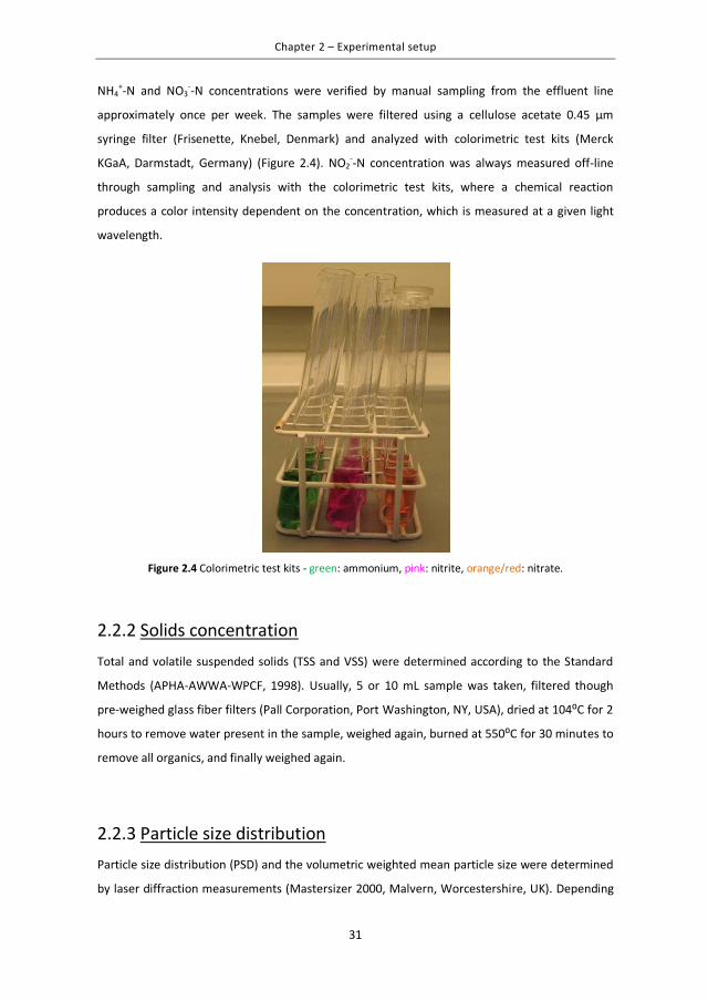
2.2 MEASUREMENTS AND ANALYSES ....................................................................................... 30 2.2.1 N analyses .......................................................................................................................... 30 2.2.2 Solids concentration ........................................................................................................... 31 2.2.3 Particle size distribution ...................................................................................................... 31 2.2.4 Oxygen transfer coefficient (kLa) ......................................................................................... 32 2.2.5 Microbiological analysis ...................................................................................................... 32
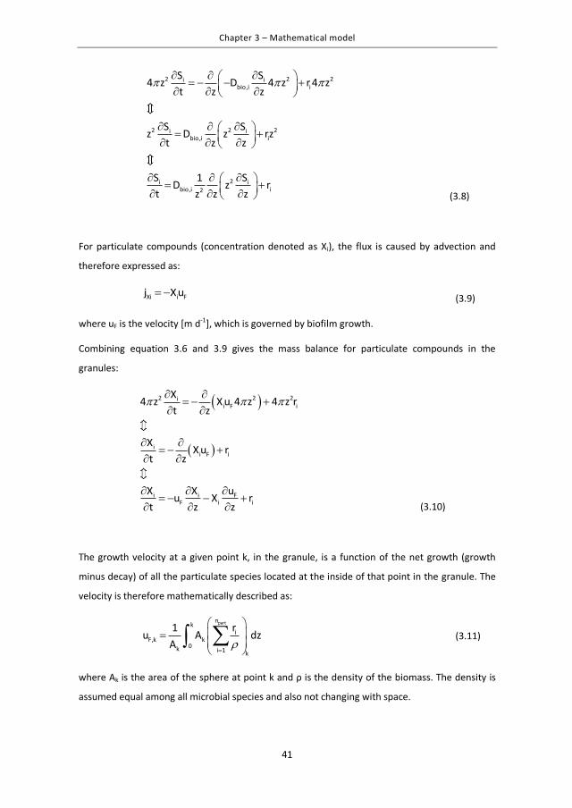
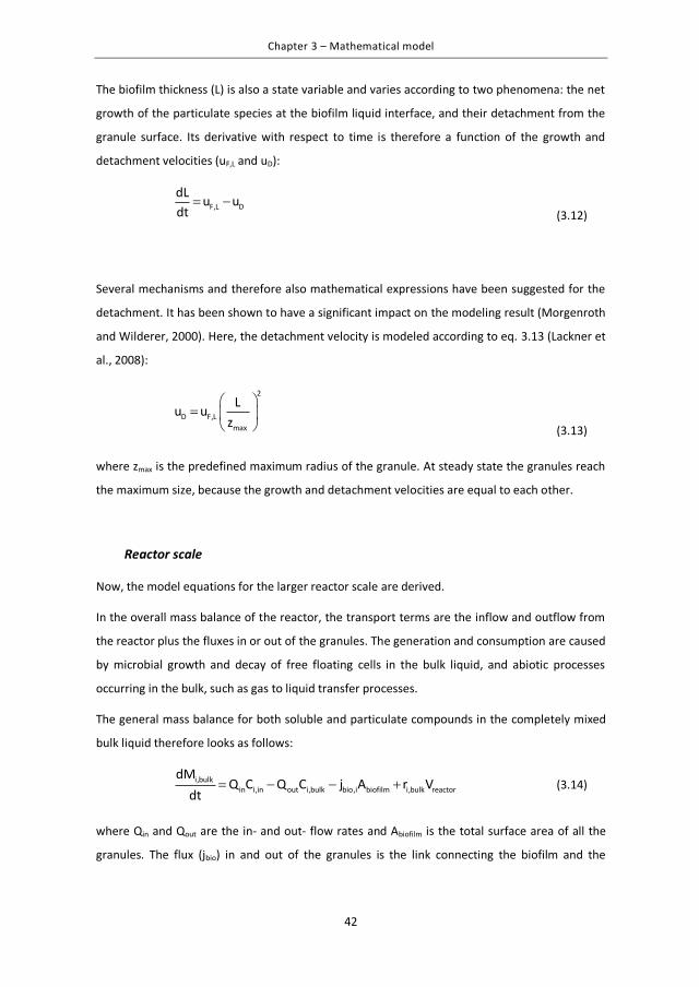
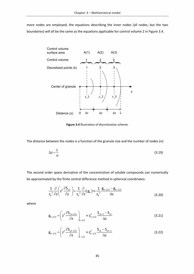
3 MATHEMATICAL MODEL ....................................................................................... 35
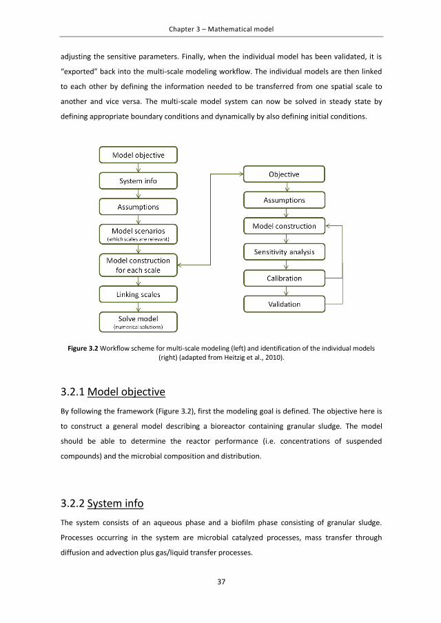
3.1 CONCEPTUAL MODEL ...................................................................................................... 35 3.2 MODEL DEVELOPMENT FRAMEWORK ................................................................................. 36
3.2.1 Model objective .................................................................................................................. 37 3.2.2 System info ......................................................................................................................... 37 3.2.3 Assumptions ....................................................................................................................... 38 3.2.4 Model equations ................................................................................................................. 38 3.2.5 Linking scales...................................................................................................................... 43 3.2.6 Model summary ................................................................................................................. 44
10
ix
3.2.7 Numerical solutions ............................................................................................................ 44 3.2.8 Model solving ..................................................................................................................... 48
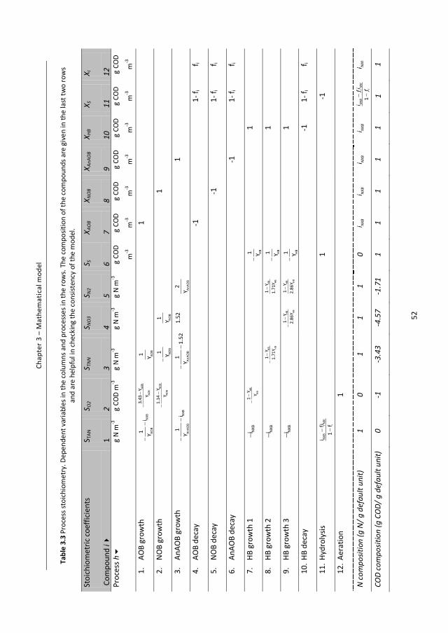
3.3 MODEL APPLIED TO CANR .............................................................................................. 48 3.3.1 Model states and variables ................................................................................................. 48 3.3.2 Model processes ................................................................................................................. 49 3.3.3 Reactor operation – CSTR vs. SBR ........................................................................................ 56 3.3.4 Model solution for the CANR system ................................................................................... 57
PART II - Simulation, Scenario, and Sensitivity Analyses
4 SENSITIVITY ANALYSIS: INFLUENCE OF MASS TRANSFER VERSUS MICROBIAL KINETICS ....................................................................................................................... 61
4.2.1 Step 1: System description .................................................................................................. 63 4.2.2 Step 2: Model description .................................................................................................... 64 4.2.3 Step 3: Uncertainty analysis ................................................................................................ 66 4.2.4 Step 4: Linear regression of Monte Carlo simulations ........................................................... 67
4.3 RESULTS AND DISCUSSION ............................................................................................... 68 4.3.1 Steady state bulk concentrations and microbial composition ............................................... 68 4.3.2 Effect of oxygen load on bulk concentrations and microbial composition ............................. 72 4.3.3 Effect of granule size on bulk concentrations and microbial composition.............................. 73 4.3.4 Effect of high N loading on bulk concentrations and microbial composition ......................... 76 4.3.5 Summarizing insights: Impact of operational conditions on N removal rates ........................ 77
7 DEVELOPMENT OF NOVEL CONTROL STRATEGIES: A PROCESS ORIENTED APPROACH ................................................................................................................. 115
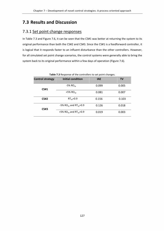
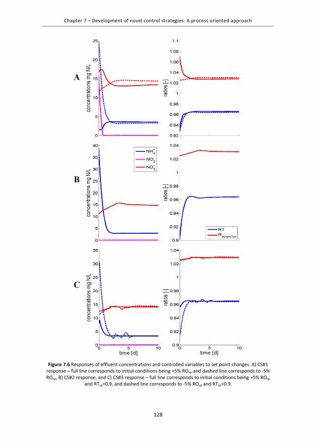
7.1 INTRODUCTION............................................................................................................ 116 7.2 A PROCESS ORIENTED APPROACH TO CONTROLLER DESIGN ................................................... 117 7.3 RESULTS AND DISCUSSION ............................................................................................. 127
7.3.1 Set point change responses ............................................................................................... 127 7.3.2 Input disturbances: step change analyses .......................................................................... 129 7.3.3 Controller response to dynamic influent profile ................................................................. 131
7.4 CONCLUSIONS AND OUTLOOK ......................................................................................... 132
8 EXPERIMENTAL VALIDATION OF A NOVEL CONTROL STRATEGY ......................... 133
8.1 INTRODUCTION............................................................................................................ 134 8.2 MATERIAL AND METHODS.............................................................................................. 134
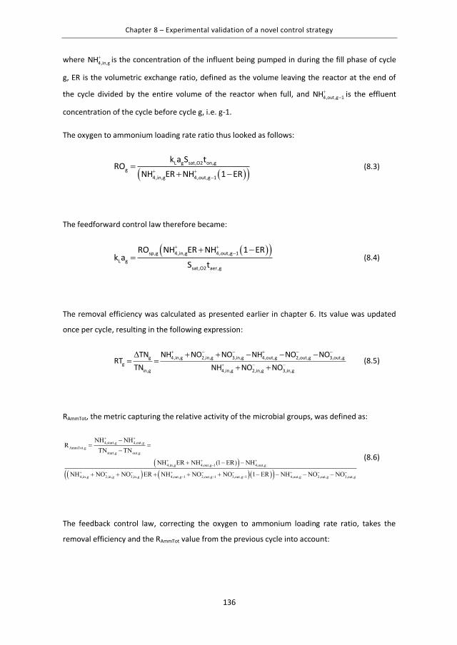
8.2.1 Reactor features and operation ........................................................................................ 134 8.2.2 Measurements and actuator ............................................................................................. 135 8.2.3 Structure of the controller ................................................................................................. 135 8.2.4 Design of control performance experiments ...................................................................... 140
8.3 RESULTS ..................................................................................................................... 142 8.3.1 Set point change response ................................................................................................ 142 8.3.2 Responses to influent ammonium disturbances ................................................................. 143 8.3.3 Dynamic influent response ................................................................................................ 145
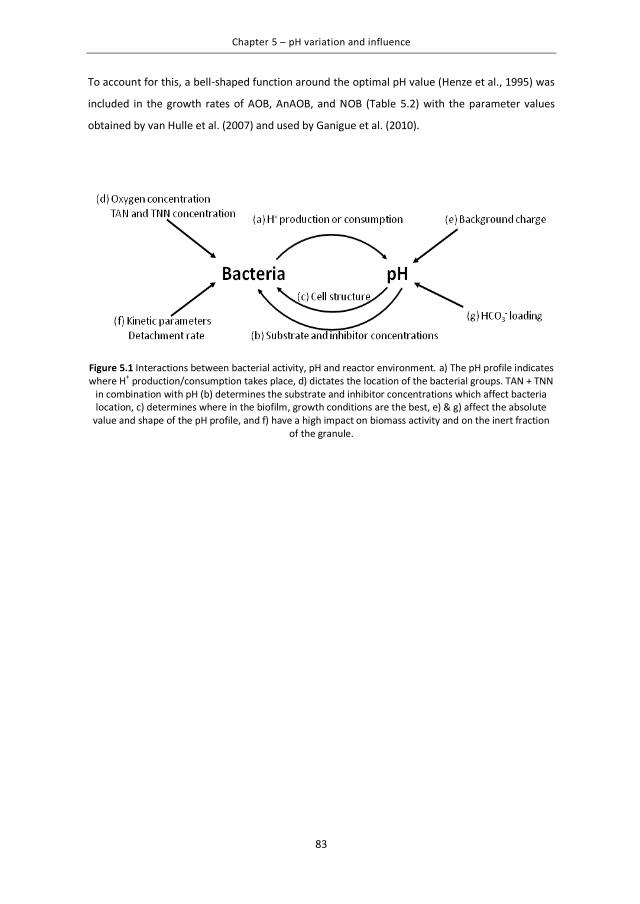
In a WWTP, biological nitrification takes place in aerated activated sludge tanks (indicated in
Figure 1.2B).
Figure 1.1 The inorganic nitrogen cycle. 1. Nitritation, 2. Nitratation, 3. Denitrification, 4. Anammox, 5. N fixation. The numbers in between the parentheses behind the compounds indicate the oxidation state of
the nitrogen atom.
17
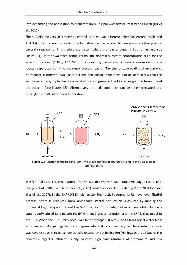
Chapter 1 - Introduction
6
Anoxic Aerated
Biological treatment Secondary clarifier
Effluent
Anaerobicdigester
Biogas
CANRReject water
Influent
Return sludge
Org. C dosing
Internal recirculation
Sludge
A B
C Sludgedewatering
Figure 1.2 Schematic diagram of a typical wastewater treatment plant (WWTP) with biological nitrogen removal (BNR), sludge digestion, and side-stream treatment. A) Anoxic denitrification tank, B) Aerobic
nitrification tank, and C) CANR of the sludge digester liquor.
The rates, at which AOB and NOB convert nitrogen, are influenced by many different
environmental factors. Manipulation of these factors has been sought to control the relative
abundance of the microbial groups in a mixed culture community. Temperature, hydraulic
retention time (HRT), sludge retention time (SRT), pH and alkalinity, inhibiting compounds, and
substrate concentrations are among the most important factors (Gujer, 2010).
The HRT control concept uses the fact that at high temperatures (above 15-20⁰C) AOB have a
higher specific growth rate than NOB, whereas the opposite is true at low temperatures
(Hellinga et al., 1998). The difference in specific growth rates can be utilized by choosing a
sufficiently low SRT to wash out NOB from the system, while retaining AOB in the system (Pollice
et al., 2002). This can relatively easily be done in continuously operated suspended sludge
systems, where there is no biomass retention and the SRT is equal to the HRT. However this
strategy becomes more difficult to administer in attached growth, sedimentation, or membrane
based systems in which solids, and thus the bacteria, are retained to a higher degree in the
system.
pH directly affects nitrification as it determines the relative distribution of the nitrogen species’
concentrations in the medium due to chemical acid-base equilibria. In addition, the nitrification
process itself affects the pH of the medium, because protons are produced when ammonium is
oxidized to nitrite (eq. 1.1). The speciation of the true substrates of the nitrogen compounds for
AOB and NOB has been a point of discussion for a while, with Anthonisen et al. (1976) proposing
18
Chapter 1 - Introduction
7
the unionized forms (ammonia (NH3) and nitrous acid (HNO2)) as the true substrates. pH can also
affect the concentration of inhibiting compounds. Many different concentrations have been
reported, and the speciation is also important in case of substrate or product inhibition
(Anthonisen et al. 1976; Wiesmann, 1994).
Another important factor affecting nitrification is the dissolved oxygen (DO) concentration. Even
though many different values, within a significant range of variation, have been reported for the
oxygen half saturation constants for both AOB and NOB (Wiesmann, 1994; Brockmann et al.,
2008; Lackner and Smets, 2012), there is a general trend that the half saturation constant of AOB
is lower compared to that of NOB. This means that at low DO concentrations, AOB will have a
competitive advantage over NOB. As a consequence many studies (Picioreanu et al., 1997;
Bernet et al., 2001; Chen et al., 2001; Downing and Nerenberg, 2008; Pambrun et al., 2008 to
name a few) have focused on controlling the DO concentration as a tool for obtaining partial
nitrification (i.e. nitritation without nitratation or nitrite accumulation).
Denitrification
In conventional treatment systems, the nitrification is typically followed by denitrification, where
nitrate is reduced eventually to nitrogen gas (N2) by heterotrophic bacteria (HB) (see Figure 1.1).
The process occurs under anoxic conditions and with organic carbon as electron donor. This
process takes place in multiple steps with several intermediates (eq. 1.5). A broad range of HB
exists, some of which have the ability to completely reduce nitrate to nitrogen gas, whereas
others are specialized in a specific step of the process.
NO3- → NO2
- → NO → N2O → N2 (1.5)
Different configurations of nitrification-denitrification can be implemented in the biological
treatment train at a WWTP. One common configuration is an anoxic tank followed by an aerated
tank with an internal recirculation stream carrying nitrate from the aerobic tank back to the
anoxic tank, where the nitrate is denitrified (see Figure 1.2A+B).
Depending on the wastewater composition, it might be necessary to supply external organic
carbon to the anoxic stage in order to ensure complete denitrification (Tchobanoglous et al.,
2003).
A detailed understanding of the denitrification mechanism, the substrate preference and
competition, and the bacteria involved remains somewhat unclear due to the complexity of the
19
Chapter 1 - Introduction
8
process (Sin et al., 2008c). Since heterotrophic activity is not the focus of this study, the reader is
referred to the reviews of Peng and Zhu (2006) and Sin et al. (2008c) for discussion of the status
of the understanding, operation, and control of this process.
Anaerobic ammonium oxidation (Anammox)
In the anammox process, ammonium is oxidized by using nitrite as electron acceptor, to form
nitrogen gas and a bit of nitrate. This process is performed by anaerobic ammonium oxidizing
bacteria (AnAOB). A simplified (1.6) and a complete (1.7) version of the process stoichiometry is
As can be seen in equation 1.7, in practice, the stoichiometry of ammonium to nitrite is 1 to
1.12. Most of the nitrogen is converted to N2, but about 6-7% of the converted nitrogen can be
found as nitrate, and the rest is incorporated in new biomass that is produced during growth.
The possible existence of AnAOB was first mentioned in the article “Two lithotrophs missing in
nature” (Broda, 1977), but was not proved existing until the 1990s (Mulder et al., 1995; van de
Graaf et al., 1995). Most of the identified AnAOB belong to the bacterial division
Planctomycetales (Kuenen, 2008). AnAOB have a characteristic bright red color, which is related
to their high production of cytochrome C (Jetten et al., 1999). Since the discovery of the AnAOB,
almost two decades ago, they have been found to be present in many WWTPs around the world
and in natural redox-stratified ecosystems, such as in sea sediments. It is estimated that up to
35% of the natural nitrogen turnover in the marine environment is through the anammox
process (Dalsgaard et al., 2003). Thus, this process is of great significance both in engineered
systems, as well as in the natural nitrogen cycle.
AnAOB are extremely slow growing with a doubling time of approximately 11 days (Strous et al.,
1998). They are very sensitive toward certain compounds and are inhibited by oxygen and nitrite
(Strous et al., 1999). Since the process is catalyzed by an obligate anoxic microorganism, oxygen
has an inhibiting effect on AnAOB already at a concentration of 0.2 mg O2 L-1 (Jung et al., 2007).
However, it has been found that AnAOB can recover their activity after exposure to low oxygen
20
Chapter 1 - Introduction
9
concentrations (Strous et al., 1997; Egli et al., 2001), thus the inhibition is probably somewhat
reversible.
Complete autotrophic nitrogen removal (CANR) is the combination of aerobic (eq. 1.1) and
anaerobic (eq. 1.6) ammonium oxidation (see eq. 1.8), and can therefore be described by the
simplified version below:
2NH4+ +1.5O2 → N2 + 2H+ + 3H2O (1.8)
1.1.2 Why use complete autotrophic nitrogen removal? As the name gives away, the CANR process is completely autotrophic, which means that the
microorganisms assimilate inorganic compounds as their carbon source. Since only 53% of the
influent ammonium has to be converted to nitrite to obtain CANR, the oxygen requirement is
1.83 g O2 (g N)-1 as opposed to 4.30 g O2 (g N)-1, which is required for complete nitrification (see
Table 1.1). The organic carbon requirement, measured as chemical oxygen demand (COD), for N
removal is 8.67 g COD (g N removed)-1 in complete nitrification-denitrification, whereas it is 0 g
COD (g N removed)-1 in CANR. This is an advantage, because organic carbon, e.g. in the form of
methanol, often is added in conventional treatment to reach complete denitrification of nitrate
(Tchobanoglous et al., 2003), and thus comprises an extra operational cost. Also the sludge
production is reduced significantly from 4.27 g biosolids (g N removed)-1 in the nitrification-
denitrification process to 0.14 g biosolids (g N removed)-1 in CANR. This is due to the relatively
low biomass yield of the AOB and AnAOB (Strous et al., 1999) compared to the yield of
heterotrophic denitrifiers (Henze et al., 2000). As can be seen in Table 1.1, the shortcut
nitrification-denitrification is superior to complete nitrification-denitrification with respect to
oxygen consumption, organic carbon requirement, and sludge production. However, the CANR is
still significantly more efficient than the short-cut pathway.
Table 1.1 Comparison of substrate requirements and sludge production for conventional nitrification-denitrification, shortcut nitrification-denitrification, and CANR, when considering the stoichiometries given
AnAOB growth yield YAnAOB 0.159 (0.07) g COD (g N)-1 (mol C (mol N)-1) (Strous et al., 1998)
HB growth yield YHB 0.67 g COD (g COD)-1 (Henze et al., 2000) (ASM1)
Inert content in biomass fi 0.08 g COD (g COD)-1 (Henze et al., 2000) (ASM1)
Nitrogen content in inert iNXI 0.06 g N (g COD)-1 (Henze et al., 2000) (ASM1)
Nitrogen content in biomass iNXB 0.086 g N (g COD)-1 (Henze et al., 2000) (ASM1)
Table 3.7 Biofilm and mass transfer parameters and their default values.
Parameter Symbol Value Unit Reference
Biomass density ρ 50000 g COD m-3 (Koch et al., 2000)
Biofilm porosity θ 0.75 - (Koch et al., 2000)
Max granule radius zmax 0.001 m (Koch et al., 2000; Vlaeminck et al., 2009)
Boundary layer thickness LB 10-5-10-4 m (Nicolella et al., 1998)
Hydrolysis rate kH 3e-0.110(293-T) day-1 (Henze et al., 2000) (ASM1)
Hydrolysis half saturation constant KX 0.3e-0.110(293-T) g COD (g COD)-1 (Henze et al., 2000) (ASM1)
Diffusivity of Ammonium in water DNH4 1.7e-4 m2 day-1 (Perry and Green, 1997)
Diffusivity of Nitrite in water DNO2 2.6e-4 m2 day-1 (Perry and Green, 1997)
Diffusivity of Nitrate in water DNO3 2.6e-4 m2 day-1 (Perry and Green, 1997)
Diffusivity of Oxygen in water DO2 2.2e-4 m2 day-1 (Perry and Green, 1997)
Diffusivity of nitrogen gas in water DN2 1.6e-4 m2 day-1 (Perry and Green, 1997)
Diffusivity of Bicarbonate in water Dalk 1.7e-4 m2 day-1 (Perry and Green, 1997)
Diffusivity of organic matter in water DS 1e-4 m2 day-1 (Hao and van Loosdrecht, 2004)
Ratio biofilm/water diffusivity f 0.75 -
Nitric acid dissociation constant pKa 3.25 -
Ammonium dissociation constant pKa 9.25 -
67
Chapter 3 – Mathematical model
56
3.3.3 Reactor operation – CSTR vs. SBR The abovementioned model can be used to simulate both continuous systems and systems of a
more discrete nature such as fed-batch reactors or SBRs.
In a CSTR type system, influent and effluent are continuously fed to and leaving the system, and
the bulk liquid is continuously aerated. The bulk liquid volume will thus be constant and its
derivative will be equal to zero:
reactordV0
dt (3.35)
The mass balance of the compounds in the bulk liquid can therefore be simplified to:
i,bulk in i,in out i,bulk bio,ii,bulk
reactor
dC Q C Q C j Ar
dt V (3.36)
where Vreactor, Qin, and Qout are constants.
In the SBR system, the model structure is the same, but some parameters change value from
one phase to another. An SBR cycle consists of the following phases: Fill, reaction, settling, draw,
and idle, as outlined in the description of the experimental setup in the previous chapter 2. Qin
has a certain value during the fill phase and is zero during the other phases. The same applies to
Qout, which only has a positive value during the draw phase, but is zero during the other phases.
Finally the aeration, in the form of the value of the mass transfer coefficient (kLa), is only active
during the reaction phase and kLa has a value of zero during the other phases (see Figure 3.5).
Figure 3.5 Schematic illustration of operational parameters affected by the SBR operation.
68
Chapter 3 – Mathematical model
57
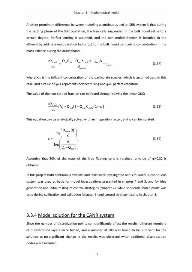
Another prominent difference between modeling a continuous and an SBR system is that during
the settling phase of the SBR operation, the free cells suspended in the bulk liquid settle to a
certain degree. Perfect settling is assumed, and the non-settled fraction is included in the
effluent by adding a multiplication factor (ϕ) to the bulk liquid particulate concentration in the
mass balance during the draw phase:
i,bulk in i,in out i,bulk bio,ii,bulk
reactor
dX Q X Q X j Ar
dt V (3.37)
where Xi,in is the influent concentration of the particulate species, which is assumed zero in this
case, and a value of ϕ=1 represents perfect mixing and ϕ=0 perfect retention.
The value of the non-settled fraction can be found through solving the linear ODE:
i,bulk0 out out i,bulk
dXV Q t Q X 1
dt (3.38)
This equation can be analytically solved with an integration factor, and ϕ can be isolated:
i,bulk
0
0
0 out
X (t)log
XVlog
V Q t
(3.39)
Assuming that 80% of the mass of the free floating cells is retained, a value of ϕ=0.32 is
obtained.
In this project both continuous systems and SBRs were investigated and simulated. A continuous
system was used as basis for model investigations presented in chapter 4 and 5, and for idea
generation and initial testing of control strategies (chapter 7), while sequential batch mode was
used during calibration and validation (chapter 6) and control strategy testing in chapter 8.
3.3.4 Model solution for the CANR system Since the number of discretization points can significantly affect the results, different numbers
of discretization layers were tested, and a number of 100 was found to be sufficient for the
solution as no significant change in the results was observed when additional discretization
nodes were included.
69
Chapter 3 – Mathematical model
58
70
59
PART II - Simulation, Scenario, and Sensitivity Analyses
This part presents the results of the simulation studies of the CANR process, which were aimed
at gaining a better understanding of the mechanisms and interactions affecting the process. In
chapter 4, the relative importance of microbial kinetics and mass transfer was investigated
through a global sensitivity analysis study performed under a number of different operation
scenarios. In chapter 5, the effect of including pH as a variable in the system (instead of
assuming it constant) was investigated by developing a pH model and an effective solution
strategy.
71
60
72
Chapter 4 – Sensitivity analysis: Influence of mass transfer versus microbial kinetics
61
4 Sensitivity analysis: Influence of mass transfer versus microbial kinetics
Summary
A comprehensive global sensitivity analysis was conducted under a range of operating
conditions. The relative importance of mass transfer resistance versus kinetic parameters was
studied and found to depend on the operating regime as follows: When operating under the
optimal loading ratio of 1.90 (g O2 m-3 d-1)/(g N m-3 d-1), the system was influenced by mass
transfer (10% impact on nitrogen removal) and performance was limited by AOB activity (75%
impact on nitrogen removal), while operating above the optimal loading ratio, AnAOB activity
was limiting (68% impact on nitrogen removal). In that case, the negative effect of oxygen mass
transfer had an impact of 15% on nitrogen removal. Summarizing such quantitative analyses led
to formulation of an optimal operation window, which serves as a valuable tool for diagnosis of
performance problems and identification of optimal solutions in nitritation-anammox
applications.
73
Chapter 4 – Sensitivity analysis: Influence of mass transfer versus microbial kinetics
62
4.1 Introduction A better understanding of which mechanisms and which process steps control and affect the
microbial community composition and the process performance is essential for future operation
and optimization of the nitrogen removal process.
Previous contributions have attempted to identify the key phenomena involved in the operation
and establishment of microbial communities based on local sensitivity analysis studies (Hao et
al., 2002a; Terada et al., 2007). In these modeling studies, external mass transfer resistance was
neglected and only kinetic and biomass related parameters were considered. The relative
importance of the mass transfer and its interaction with microbial kinetics were therefore not
examined. It has previously been shown that inclusion of external mass transfer has an impact
on the parameter identifiability in nitrifying biofilms (Brockmann et al., 2008), and it is therefore
of interest to investigate the sensitivity towards this mass transfer. To overcome the limitations
of the local sensitivity analysis and the lack of the external mass transfer resistance of previous
studies and to expand the boundary of the process analysis, this study use global sensitivity
analysis with a significantly expanded scope. The global sensitivity analysis, e.g. linear regression
of Monte Carlo (MC) simulations, has previously been demonstrated as a useful tool to diagnose
the state of the system, obtain valuable insights, and identify bottlenecks in a process (Sin et al.,
2011).
The aim of the work presented in this chapter was, therefore, to elucidate which mechanisms
were the most influential on the process performance of a single-stage complete autotrophic
nitrogen removing granular sludge reactor. Specific emphasis was put on diagnosing the key step
in the overall process for a given set of operating conditions. Mass transfer parameters and
microbial kinetic parameters and their individual impacts on the concentrations of substrates,
intermediates, products, and bacterial groups were therefore investigated for several scenarios
considering different influent conditions, different operational strategies and different granule
sizes. To this end, a model-based methodology that employs global sensitivity analysis
techniques along with the 1-D multi-scale multi-species granular biofilm model from chapter 3
was developed and used.
74
Chapter 4 – Sensitivity analysis: Influence of mass transfer versus microbial kinetics
63
4.2 Methods Before carrying out the sensitivity analysis, scenarios of interest were first identified, and
appropriate models were set up. The key steps in the uncertainty and sensitivity analysis were
defined, which included identifying and characterizing parameter uncertainty, sampling of the
defined parameter space, and performing Monte Carlo simulations (Sin et al., 2009). The
sensitivity of the uncertain parameters was then quantified by constructing linear models of
selected model outputs, and finally the sensitivity analysis results were evaluated by putting
them into context with the system information of the given scenario.
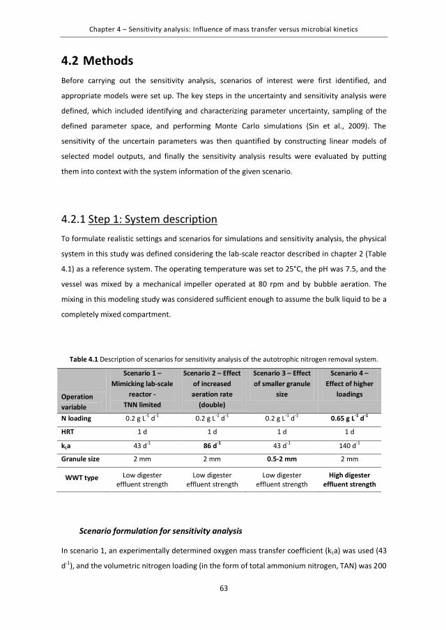
4.2.1 Step 1: System description To formulate realistic settings and scenarios for simulations and sensitivity analysis, the physical
system in this study was defined considering the lab-scale reactor described in chapter 2 (Table
4.1) as a reference system. The operating temperature was set to 25°C, the pH was 7.5, and the
vessel was mixed by a mechanical impeller operated at 80 rpm and by bubble aeration. The
mixing in this modeling study was considered sufficient enough to assume the bulk liquid to be a
completely mixed compartment.
Table 4.1 Description of scenarios for sensitivity analysis of the autotrophic nitrogen removal system.
Operation variable
Scenario 1 – Mimicking lab-scale
reactor - TNN limited
Scenario 2 – Effect of increased aeration rate
(double)
Scenario 3 – Effect of smaller granule
size
Scenario 4 – Effect of higher
loadings
N loading 0.2 g L-1 d-1 0.2 g L-1 d-1 0.2 g L-1 d-1 0.65 g L-1 d-1
HRT 1 d 1 d 1 d 1 d
kLa 43 d-1 86 d-1 43 d-1 140 d-1
Granule size 2 mm 2 mm 0.5-2 mm 2 mm
WWT type Low digester effluent strength
Low digester effluent strength
Low digester effluent strength
High digester effluent strength
Scenario formulation for sensitivity analysis
In scenario 1, an experimentally determined oxygen mass transfer coefficient (kLa) was used (43
d-1), and the volumetric nitrogen loading (in the form of total ammonium nitrogen, TAN) was 200
75
Chapter 4 – Sensitivity analysis: Influence of mass transfer versus microbial kinetics
64
g N m-3 d-1. The solids concentration was maintained at 3.14 g VSS L-1 in the reactor, which is
within the range of lab-scale (Vazquez-Padin et al., 2009; Figueroa et al., 2012) and full-scale
observations (Joss et al., 2009). This solids concentration was used as a reference in the
simulations and scenarios for the sensitivity analysis. The mass transfer coefficients were
determined using a semi-empirical correlation for mixed reactors with aeration (Nicolella et al.,
1998). The average thickness of the external mass transfer boundary layer (LB) was estimated to
be 64 μm, which is also within the range reported in attached growth experiments (Masic et al.,
2010). Three additional scenarios were evaluated (Table 4.1). In scenario 2, the effect of oxygen
supply was investigated by doubling the mass transfer coefficient. In scenario 3, the effect of
granule sizes was investigated. Lastly, the effect of high influent loading was investigated in
scenario 4. In the latter scenario, the oxygen supply was simultaneously increased by increasing
the kLa to 140 d-1.
4.2.2 Step 2: Model description The model of the CANR process operated as a continuous system, described in chapter 3, was
used as basis for the analysis.
The steady state concentrations in the biofilm and the bulk liquid were found by simulating the
system for a sufficiently long time (in this case 5000 days) using the default parameter values
shown in Table 4.2. These steady state concentrations were used as initial conditions for the
mass balance equations for each of the scenarios.
76
Chapter 4 – Sensitivity analysis: Influence of mass transfer versus microbial kinetics
65
Table 4.2 Parameters included in the uncertainty analysis and the classification of their uncertainties.
No. Parameter Default value at 20⁰C
Unit Reference Uncertainty class
1 μmax,AOB 0.80 day-1 Hao et al., 2002b 2 2 KO2,AOB 0.30 g O2 m-3 Wiesmann, 1994 3 3 KNH3,AOB 0.04 g N m-3 Wiesmann, 1994 3 4 KHNO2,AOB 2.04 g N m-3 Van Hulle et al., 2007 3 5 bAOB 0.05 day-1 Hao et al., 2002b 2 6 μmax,NOB 0.79 day-1 Hao et al., 2002b 2 7 KO2,NOB 1.10 g O2 m-3 Wiesmann, 1994 3 8 KHNO2,NOB 3.09e-4 g N m-3 Wiesmann, 1994 3 9 bNOB 0.033 day-1 Hao et al., 2002b 2 10 μmax,AnAOB 0.028 day-1 Hao et al., 2002b 2 11 KO2,AnAOB 0.01 g O2 m-3 Strous et al., 1999 3 12 KNH3,AnAOB 1.20e-3 g N m-3 Strous et al., 1998 3 13 KHNO2,AnAOB 2.81e-6 g N m-3 Strous et al., 1998 3 14 bAnAOB 0.001 day-1 Hao et al., 2002b 2 15 μmax,HB 6.00 day-1 Henze et al., 2000(ASM1) 2 16 KO2,HB 0.20 g O2 m-3 Henze et al., 2000 (ASM1) 3 17 KS,HB 20.0 g COD m-3 Henze et al., 2000 (ASM1) 3 18 KTNN,HB 0.50 g N m-3 Henze et al., 2000 (ASM1) 3 19 KNO3,HB 0.50 g N m-3 Henze et al., 2000 (ASM1) 3 20 KTAN,HB 0.01 g N m-3 Henze et al., 2000 (ASM3) 3 21 ηHB 0.80 - Henze et al., 2000 (ASM1) 2 22 bHB 0.62 day-1 Henze et al., 2000 (ASM1) 1 23 YAOB 0.21 g COD (g N)-1 Wiesmann, 1994 1 24 YNOB 0.059 g COD (g N)-1 Wiesmann, 1994 1 25 YAnAOB 0.159 g COD (g N)-1 Strous et al., 1998 1 26 YHB 0.67 g COD (g COD)-1 Henze et al., 2000 (ASM1) 1 27 fi 0.08 g COD (g COD)-1 Henze et al., 2000 (ASM1) 2 28 iNXI 0.06 g N (g COD)-1 Henze et al., 2000 (ASM1) 2 29 iNXB 0.086 g N (g COD)-1 Henze et al., 2000 (ASM1) 2 30 kH 3.00 day-1 Henze et al., 2000 (ASM1) 1 31 KX 0.30 g COD (g COD)-1 Henze et al., 2000 (ASM1) 1 32 DNH4 1.70e-4 m2 day-1 Perry and Green, 1997 2 33 DNO2 2.60e-4 m2 day-1 Perry and Green, 1997 2 34 DO2 2.20e-4 m2 day-1 Perry and Green, 1997 2 35 DNO3 2.60e-4 m2 day-1 Perry and Green, 1997 2 36 DN2 1.60e-4 m2 day-1 Perry and Green, 1997 2 37 DS 1.00e-4 m2 day-1 Perry and Green, 1997 2 38 LB 6.40e-5 m Nicolella et al., 1998 3
77
Chapter 4 – Sensitivity analysis: Influence of mass transfer versus microbial kinetics
66
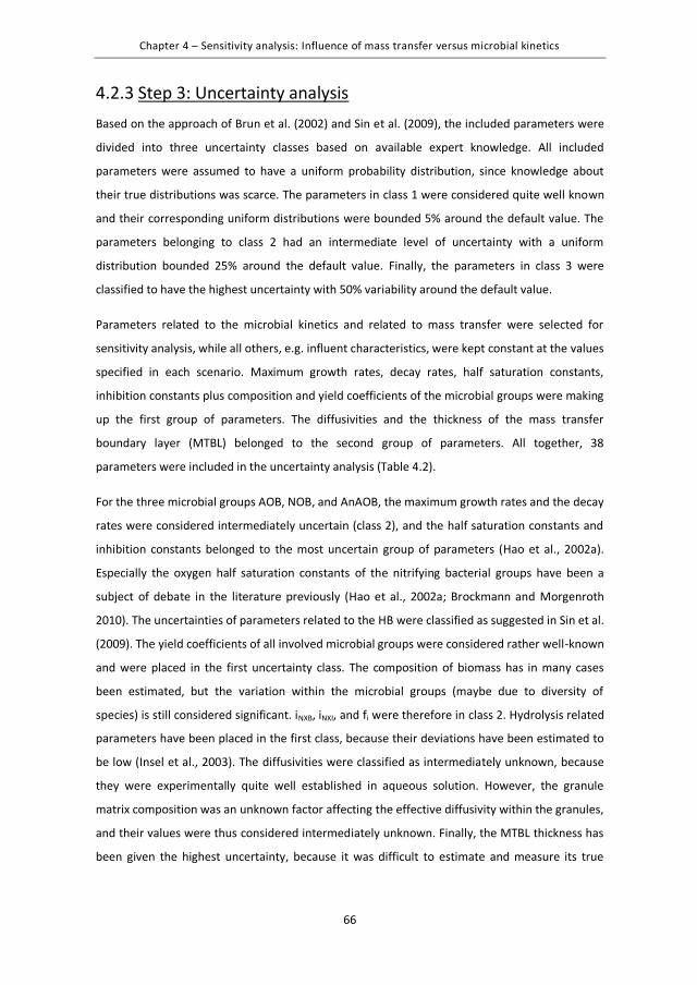
4.2.3 Step 3: Uncertainty analysis Based on the approach of Brun et al. (2002) and Sin et al. (2009), the included parameters were
divided into three uncertainty classes based on available expert knowledge. All included
parameters were assumed to have a uniform probability distribution, since knowledge about
their true distributions was scarce. The parameters in class 1 were considered quite well known
and their corresponding uniform distributions were bounded 5% around the default value. The
parameters belonging to class 2 had an intermediate level of uncertainty with a uniform
distribution bounded 25% around the default value. Finally, the parameters in class 3 were
classified to have the highest uncertainty with 50% variability around the default value.
Parameters related to the microbial kinetics and related to mass transfer were selected for
sensitivity analysis, while all others, e.g. influent characteristics, were kept constant at the values
specified in each scenario. Maximum growth rates, decay rates, half saturation constants,
inhibition constants plus composition and yield coefficients of the microbial groups were making
up the first group of parameters. The diffusivities and the thickness of the mass transfer
boundary layer (MTBL) belonged to the second group of parameters. All together, 38
parameters were included in the uncertainty analysis (Table 4.2).
For the three microbial groups AOB, NOB, and AnAOB, the maximum growth rates and the decay
rates were considered intermediately uncertain (class 2), and the half saturation constants and
inhibition constants belonged to the most uncertain group of parameters (Hao et al., 2002a).
Especially the oxygen half saturation constants of the nitrifying bacterial groups have been a
subject of debate in the literature previously (Hao et al., 2002a; Brockmann and Morgenroth
2010). The uncertainties of parameters related to the HB were classified as suggested in Sin et al.
(2009). The yield coefficients of all involved microbial groups were considered rather well-known
and were placed in the first uncertainty class. The composition of biomass has in many cases
been estimated, but the variation within the microbial groups (maybe due to diversity of
species) is still considered significant. iNXB, iNXI, and fi were therefore in class 2. Hydrolysis related
parameters have been placed in the first class, because their deviations have been estimated to
be low (Insel et al., 2003). The diffusivities were classified as intermediately unknown, because
they were experimentally quite well established in aqueous solution. However, the granule
matrix composition was an unknown factor affecting the effective diffusivity within the granules,
and their values were thus considered intermediately unknown. Finally, the MTBL thickness has
been given the highest uncertainty, because it was difficult to estimate and measure its true
78
Chapter 4 – Sensitivity analysis: Influence of mass transfer versus microbial kinetics
67
value due to its high sensitivity to the hydrodynamic conditions around the granule (Masic et al.,
2010; Boltz et al., 2011).
The above defined parameter space was sampled by the Latin Hypercube Sampling (LHS)
method (Iman and Conover, 1982). The parameters were considered to be uncorrelated due to
unavailability of the information on the correlation matrix. As the sampling number from the
joint probability distributions of the uncertain parameter space, 500 samples were taken and
used for Monte Carlo simulations of the system for a period of 5000 days, from which the steady
state model outputs were obtained. Similar time periods needed to reach steady state in such
systems have been reported elsewhere (Volcke et al., 2010).
The model outputs formed the basis of the subsequent sensitivity analysis.
4.2.4 Step 4: Linear regression of Monte Carlo simulations The sensitivity was found by performing linear regression on each of the model outputs. A first
order linear multivariate model was fitted to the model outputs (yk), which was relating it to the
parameter values (θi) (Saltelli et al., 2008):
, ,reg k k k i ii
y a b (4.1)
where ak and bk,i are linear regression coefficients. The standardized linear regression
coefficients (SRCs), βk,i, were obtained by making eq. 4.1 non-dimensional by mean-centered
sigma-scaling, where μyk and i are the mean values and σyk and i are the standard deviations
of the model outputs and input parameters, respectively:
,,
reg k yk i ik i
iyk i
y (4.2)
The linear coefficient (bk,i) is related to the standardized coefficient in the following way:
, ,i
k i k iyk
b (4.3)
79
Chapter 4 – Sensitivity analysis: Influence of mass transfer versus microbial kinetics
68
If the model was linearly additive, then 2 1ii
for each model output, and 2i would
represent the relative variance contribution of parameter i and thus be giving a measure of the
importance of the model output. In this study the model was assumed linear if the squared
coefficient of correlation (R2) between the Monte Carlo simulation output (yk) and the regressed
linear output (yreg,k) was above 0.7. A parameter was considered sensitive or significant when
0.1i , meaning that the parameter approximately contributed with at least 1% of the model
output variance (Sin et al., 2011).
4.3 Results and discussion Ten selected outputs were evaluated after reaching steady state for every set of parameter
values. To obtain more details on how the entire process was affected, the bulk concentrations
of TAN, TNN, nitrate, and DO on top of N2 (which is equal to the nitrogen removal and represents
the process performance) were selected for evaluation. The last five model outputs evaluated
were the mass fractions of the particulate species within the granules, namely the AOB, AnAOB,
NOB, HB, and the inert material, which gave information about the microbial community
composition.
4.3.1 Steady state bulk concentrations and microbial composition The steady state concentrations of soluble compounds and the granule composition, found by
simulations using the default parameter values and operation as specified in scenario 1, can be
seen in Figure 4.1A. Oxygen and TNN were depleted within the first few hundred μm, while TAN
penetrated the entire granule. HB were only present in low concentrations close to the
biofilm/bulk liquid interface, and NOB were present in negligible concentrations.
80
Chapter 4 – Sensitivity analysis: Influence of mass transfer versus microbial kinetics
69
Figure 4.1 Soluble compounds and biomass concentrations inside the granule obtained from simulations using the default parameter values. The dashed vertical line indicates the position of the biofilm/liquid
Chapter 4 – Sensitivity analysis: Influence of mass transfer versus microbial kinetics
71
Significance of microbial conversion kinetics vs. mass transfer parameters on
microbial interactions in scenario 1
In order to elucidate the mechanisms affecting the microbial composition and process
performance, the kinetic parameters were further divided according to the groups of
microorganisms they were related to. From this analysis, the microbial interactions could be
inferred. The variance of the AOB mass fraction was predominantly governed by variance of
their own kinetic parameters (see Table 4.3), which entails them not being significantly affected
by substrate competition with other organisms under these operational conditions. For the
AnAOB mass fraction, a significant amount of the variance could be assigned to the AOB
parameters (see Table 4.3), because AnAOB were dependent on AOB for production of substrate
(TNN) as electron acceptor and removal of the inhibiting oxygen. The variance of HB mainly
(43%) originated from their own kinetic parameters, but a large part (40%) could be attributed to
the AOB kinetics as well, and a smaller amount (14%) to the AnAOB kinetic parameters. This
shows that the HB mainly utilized decay products originating from AOB. The variance in the inert
mass fraction was almost solely due to AOB and AnAOB.
Overall, it can be concluded that AOB activity and TNN availability for AnAOB were the main
limiting factors for the nitrogen removal in oxygen limited systems. This is furthermore
supported by the N2 mainly being affected by AOB kinetics (see Figure 4.2). The linear model
obtained from the linear regression of the Monte Carlo simulations is valid for the given
operating point defined in scenario 1 and provides an approximation of the steady state
nitrogen removal, in the form of nitrogen gas concentration in the bulk liquid, as a function of
parameters, which had an impact of at least 5% (see eq. 4.4). The unit of the number in front of
each parameter value has the unit of g N2-N m-3 in the bulk per unit of the given parameter.
From this it can be deduced, that as AOB activity increased (μmax,AOB increased or KO2,AOB
decreased) the nitrogen removal simultaneously increased. Also noteworthy is that as the
external mass transfer resistance increased (increased LB), the performance decreased.
32 max,AOB O2,AOB AnAOB BN 4.79 13.73 K 132.5 Y 27554 L 180.5 g N/m (4.4)
83
Chapter 4 – Sensitivity analysis: Influence of mass transfer versus microbial kinetics
72
Figure 4.2 Result of sensitivity analyses for the bulk concentration of N2, which represents the process
performance. The slices are given as the sum of the squared SRCs within the given group divided by the sum of all the squared SRCs. The output could be sufficiently linearized for all scenarios except for
scenario 4.
4.3.2 Effect of oxygen load on bulk concentrations and microbial
composition In scenario 2, the volumetric mass transfer coefficient for oxygen, kLa, was doubled, which
entailed an increased oxygen loading to the system. This resulted in an increase in the bulk DO
concentration to 0.5-1.3 g O2 m-3 (in all Monte Carlo simulations), as opposed to 0.1-0.4 g O2 m-3
in scenario 1. Even at double kLa, the oxygen was depleted within the granule. The higher oxygen
supply caused the system to no longer be TNN limited (see the left hand side of Figure 4.1B), and
NOB could compete for space with the other microbial groups in the granules. Even though
AnAOB had a higher affinity for TNN than NOB, competition between the species was possible
since NOB could withstand a higher oxygen concentration. As a consequence they could occupy
a region close to the source of TNN in the granules (see Figure 4.1B). This is in line with the
findings by Hao et al. (2002a), who found that AnAOB win the competition for TNN against NOB,
when KO2,NOB/ KO2,AOB > 0.2 and KO2,NOB/ KO2,AnAOB > 3. This is, however, only valid under sufficiently
low oxygen supply conditions, as can be observed from the results obtained here.
84
Chapter 4 – Sensitivity analysis: Influence of mass transfer versus microbial kinetics
73
The sensitivity analysis results (see Appendix A2) showed that the TAN and TNN bulk
concentrations were mainly affected by the microbial kinetics and no longer by mass transfer
related parameters. While this result made sense for TNN, it was a bit surprising for TAN. The
bulk TNN concentration was no longer affected by the producer’s kinetics (AOB), but by its
consumers’ kinetics (NOB and AnAOB), which underlined, that the TNN production by AOB was
no longer a key step for the reactor performance. AOB were slightly dependent on AnAOB
kinetics, in contrast with scenario 1. Along with the TAN concentration being affected by AnAOB
kinetics, this indicates that the TAN substrate competition between AOB and AnAOB was an
important mechanism influencing the overall process.
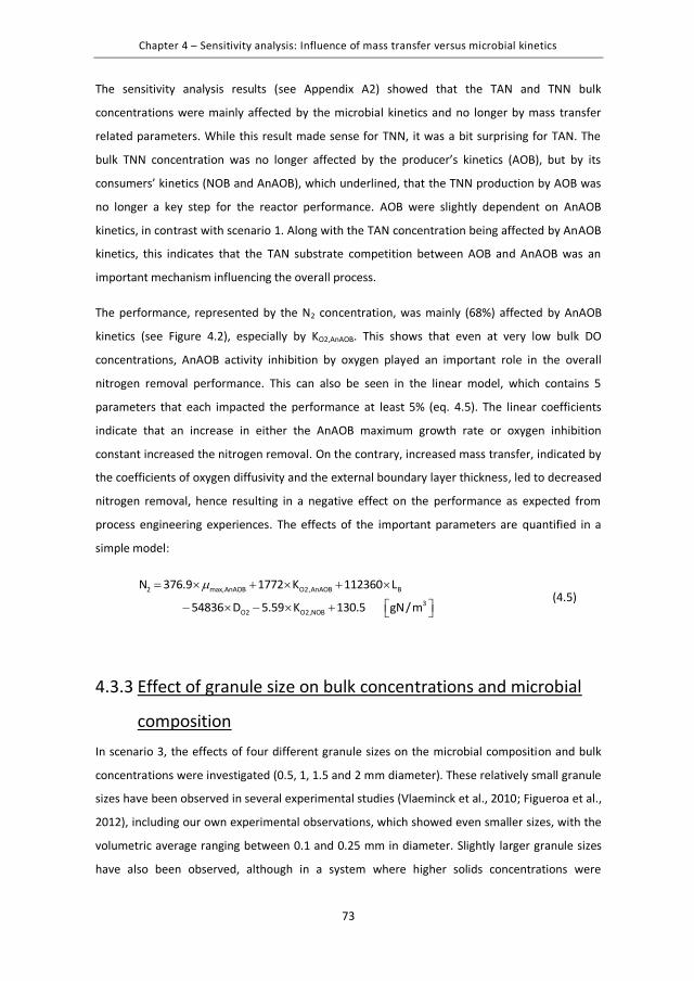
The performance, represented by the N2 concentration, was mainly (68%) affected by AnAOB
kinetics (see Figure 4.2), especially by KO2,AnAOB. This shows that even at very low bulk DO
concentrations, AnAOB activity inhibition by oxygen played an important role in the overall
nitrogen removal performance. This can also be seen in the linear model, which contains 5
parameters that each impacted the performance at least 5% (eq. 4.5). The linear coefficients
indicate that an increase in either the AnAOB maximum growth rate or oxygen inhibition
constant increased the nitrogen removal. On the contrary, increased mass transfer, indicated by
the coefficients of oxygen diffusivity and the external boundary layer thickness, led to decreased
nitrogen removal, hence resulting in a negative effect on the performance as expected from
process engineering experiences. The effects of the important parameters are quantified in a
simple model:
2 max,AnAOB O2,AnAOB B
3O2 O2,NOB
N 376.9 1772 K 112360 L
54836 D 5.59 K 130.5 gN/m (4.5)
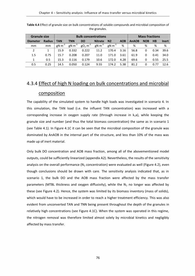
4.3.3 Effect of granule size on bulk concentrations and microbial
composition In scenario 3, the effects of four different granule sizes on the microbial composition and bulk
concentrations were investigated (0.5, 1, 1.5 and 2 mm diameter). These relatively small granule
sizes have been observed in several experimental studies (Vlaeminck et al., 2010; Figueroa et al.,
2012), including our own experimental observations, which showed even smaller sizes, with the
volumetric average ranging between 0.1 and 0.25 mm in diameter. Slightly larger granule sizes
have also been observed, although in a system where higher solids concentrations were
85
Chapter 4 – Sensitivity analysis: Influence of mass transfer versus microbial kinetics
74
observed as well (Vazquez-Padin et al., 2009). The total solids concentration was kept constant
in the different simulation scenarios by increasing the number of granules with decreasing
granule size, while assuming a constant granule density for all the granule sizes. This means that
external mass transfer resistance will decrease with increasing specific surface area of the
granules (i.e. smaller granules, higher mass transfer rate).
In line with this, the AOB mass fraction slightly increased while the bulk DO concentration
slightly decreased with decreasing size (Table 4.4 and Figure 4.3). The granule sizes investigated
showed quite similar performance results, with the overall process performance slightly
increasing with decreasing granule size (Table 4.4). This is in line with the results of Volcke et al.
(2010). However, similar to their results, this is expected only to happen when operating under
conditions where the performance is limited by AOB activity (as in scenario 1), because the
aerobic volume is increased in smaller granules, and not by AnAOB activity, for which larger
granules are expected to perform better.
The result of the sensitivity analysis was almost identical to scenario 1 (Figure 4.2), which entails
that the mass transfer was still important for AOB, TNN, and N2 at smaller granule sizes, even
though the mass transfer resistance was lowered as the specific surface area increased. The
inhibitory effect of oxygen on AnAOB activity is speculated to be the reason, which is also
reflected in the changes in the biomass composition; the smaller granules consist of higher
amounts of AnAOB (Table 4.4), but with a lower activity due to oxygen inhibition. In line with
this finding, Vlaeminck et al. (2010) showed in batch tests conducted with granules belonging to
the smallest size fraction that the specific rate of ammonium conversion by AnAOB was lower
than in larger granules. However, they also found lower abundance of AnAOB in smaller granules
than in bigger ones. This observation could be due to the particular operation history of their
OLAND reactor that affected the granule composition and physiology of the biomass (e.g. the
performance of the OLAND reactor is a combination of the performance of the different sizes of
granules). To resolve this observation, more experimental investigations on different systems
are needed. It could thus be deduced that there was no simple relationship between biomass
composition and process performance, which was also shown by Lackner et al. (2008) in a
modeling study of membrane aerated biofilm reactors.
Since the result of the sensitivity analysis was similar to the observations made in scenario 1, the
key step in the overall removal remained the AOB activity and TNN availability for AnAOB.
86
Chapter 4 – Sensitivity analysis: Influence of mass transfer versus microbial kinetics
75
Figure 4.3 Biomass distribution in granules at different granule sizes. (A) rgran = 1 mm, (B) rgran = 0.75 mm,
(C) rgran = 0.5 mm, and (D) rgran = 0.25 mm.
It can be argued that systems containing the bigger granules (2 mm in diameter) were containing
excess solids and the specific nitrogen removal rate (measured as g Nremoved g VSS-1 d-1) could
therefore be increased. The same was found by Ni et al. (2009), who found that anammox
performing granules above 1.3 mm in diameter did not perform better, but showed a lower
specific nitrogen removal rate.
An interesting observation is that as the N2 production increased with decreasing size, the bulk
nitrate concentration decreased simultaneously (Table 4.4). This may be attributed to HB
activity, which indicated that HB, even though low in numbers, had an impact on the
performance. As in scenario 1, HB grew on decay products originating from AOB, and when they
were present in higher concentration (as is the case with smaller granules with less oxygen
limitation), the HB had better conditions to grow. Thus, HB in low concentrations contributed to
a slightly better nitrogen removal through a) anoxic heterotrophic activity (denitrification) with
N2 production and nitrate removal and b) TAN assimilation for growth of HB.
87
Chapter 4 – Sensitivity analysis: Influence of mass transfer versus microbial kinetics
76
Table 4.4 Effect of granule size on bulk concentrations of soluble compounds and microbial composition of the granules.
Granule size Bulk concentrations Mass fractions Diameter Radius TAN TNN DO Nitrate N2 AOB AnAOB NOB HB Inert
mm mm gN m-3 gN m-3 gO2 m-3 gN m-3 gN m-3 % % % % %
4.3.4 Effect of high N loading on bulk concentrations and microbial
composition The capability of the simulated system to handle high loads was investigated in scenario 4. In
this simulation, the TAN load (i.e. the influent TAN concentration) was increased with a
corresponding increase in oxygen supply rate (through increase in kLa), while keeping the
granule size and number (and thus the total biomass concentration) the same as in scenario 1
(see Table 4.1). In Figure 4.1C it can be seen that the microbial composition of the granule was
dominated by AnAOB in the internal part of the structure, and less than 10% of the mass was
made up of inert material.
Only bulk DO concentration and AOB mass fraction, among all of the abovementioned model
outputs, could be sufficiently linearized (appendix A2). Nevertheless, the results of the sensitivity
analysis on the overall performance (N2 concentration) were evaluated as well (Figure 4.2), even
though conclusions should be drawn with care. The sensitivity analysis indicated that, as in
scenario 1, the bulk DO and the AOB mass fraction were affected by the mass transfer
parameters (MTBL thickness and oxygen diffusivity), while the N2 no longer was affected by
these (see Figure 4.2). Hence, the system was limited by its biomass inventory (mass of solids),
which would have to be increased in order to reach a higher treatment efficiency. This was also
evident from unconverted TAN and TNN being present throughout the depth of the granules in
relatively high concentrations (see Figure 4.1C). When the system was operated in this regime,
the nitrogen removal was therefore limited almost solely by microbial kinetics and negligibly
affected by mass transfer.
88
Chapter 4 – Sensitivity analysis: Influence of mass transfer versus microbial kinetics
77
4.3.5 Summarizing insights: Impact of operational conditions on N
removal rates To sum up the findings from all the abovementioned scenarios, the process performance as a
function of the nitrogen and oxygen loading was investigated by simulating 10 TAN loads ranging
from 100 to 1000 g N m-3 d-1 combined with 10 kLa values, ranging from 25 to 250 d-1, resulting in
100 different operational conditions. The system was simulated to steady state with these
operational conditions, and the resulting volumetric nitrogen removal rates (g N m-3 d-1) and
removal efficiencies are shown in Figure 4.4. The graphs presented serve as a two dimensional
operation window.
Figure 4.4 Process performance as N removal rate (left) and N removal efficiency (right) as a function of
the operational conditions (oxygen and N load). The locations of the four operational scenarios are shown in the left plot.
The observed optimal loading ratio was slightly higher than the theoretical ratio of the
stoichiometry of nitrogen and oxygen substrates. The theoretical stoichiometry yields a ratio of
1.83 g O2 (g N)-1, whereas the observed optimal loading ratio was here found to be 1.90 (g O2 m-3
d-1)/(g N m-3 d-1), as can be seen from Figure 4.5. This is higher than the values reported for
conventional flat biofilm and membrane aerated biofilm systems (Terada et al., 2007). In the
study of Terada et al. (2007), the optimal surface loading ratio was found to be 1.5-1.6 (g O2 m-2
d-1)/(g N m-2 d-1), which was below the theoretical value. However, the external mass transfer
resistance was neglected in that study, which under certain operational conditions plays an
important role. The different results could be caused by the presence of HB, or because the
89
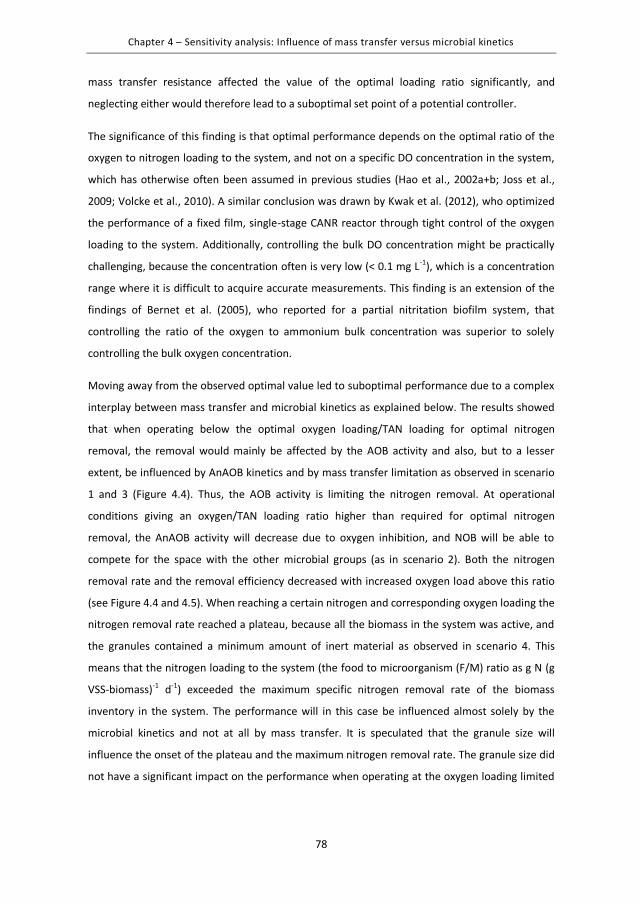
Chapter 4 – Sensitivity analysis: Influence of mass transfer versus microbial kinetics
78
mass transfer resistance affected the value of the optimal loading ratio significantly, and
neglecting either would therefore lead to a suboptimal set point of a potential controller.
The significance of this finding is that optimal performance depends on the optimal ratio of the
oxygen to nitrogen loading to the system, and not on a specific DO concentration in the system,
which has otherwise often been assumed in previous studies (Hao et al., 2002a+b; Joss et al.,
2009; Volcke et al., 2010). A similar conclusion was drawn by Kwak et al. (2012), who optimized
the performance of a fixed film, single-stage CANR reactor through tight control of the oxygen
loading to the system. Additionally, controlling the bulk DO concentration might be practically
challenging, because the concentration often is very low (< 0.1 mg L-1), which is a concentration
range where it is difficult to acquire accurate measurements. This finding is an extension of the
findings of Bernet et al. (2005), who reported for a partial nitritation biofilm system, that
controlling the ratio of the oxygen to ammonium bulk concentration was superior to solely
controlling the bulk oxygen concentration.
Moving away from the observed optimal value led to suboptimal performance due to a complex
interplay between mass transfer and microbial kinetics as explained below. The results showed
that when operating below the optimal oxygen loading/TAN loading for optimal nitrogen
removal, the removal would mainly be affected by the AOB activity and also, but to a lesser
extent, be influenced by AnAOB kinetics and by mass transfer limitation as observed in scenario
1 and 3 (Figure 4.4). Thus, the AOB activity is limiting the nitrogen removal. At operational
conditions giving an oxygen/TAN loading ratio higher than required for optimal nitrogen
removal, the AnAOB activity will decrease due to oxygen inhibition, and NOB will be able to
compete for the space with the other microbial groups (as in scenario 2). Both the nitrogen
removal rate and the removal efficiency decreased with increased oxygen load above this ratio
(see Figure 4.4 and 4.5). When reaching a certain nitrogen and corresponding oxygen loading the
nitrogen removal rate reached a plateau, because all the biomass in the system was active, and
the granules contained a minimum amount of inert material as observed in scenario 4. This
means that the nitrogen loading to the system (the food to microorganism (F/M) ratio as g N (g
VSS-biomass)-1 d-1) exceeded the maximum specific nitrogen removal rate of the biomass
inventory in the system. The performance will in this case be influenced almost solely by the
microbial kinetics and not at all by mass transfer. It is speculated that the granule size will
influence the onset of the plateau and the maximum nitrogen removal rate. The granule size did
not have a significant impact on the performance when operating at the oxygen loading limited
90
Chapter 4 – Sensitivity analysis: Influence of mass transfer versus microbial kinetics
79
regions in Figure 4.4, which was the case in scenario 3. However, if operating at the biomass
limited plateau, the size is expected to have an impact on the performance.
The removal efficiency was optimal at a loading ratio of 1.90 (g O2 m-3 d-1)/(g N m-3 d-1) and at
low nitrogen loadings (Figure 4.4). As the nitrogen loading increased, the removal efficiency
decreased due to increased AnAOB inhibition by oxygen and limitation of the biomass inventory
in the system to convert all nitrogen present in the influent (these operational conditions are
indicated in the center of Figure 4.5).
Figure 4.5 Nitrogen removal efficiency as a function of the oxygen to nitrogen loading ratio.
4.4 Conclusions In this work, phenomena that are the most influential on process performance of nitritation-
anammox granular bioreactors were computationally identified and quantified via a global
sensitivity analysis. Based on the analysis, an optimal operation window for the system was
developed, which among others, revealed that the optimal nitrogen removal performance is
critically controlled by the ratio of the oxygen supplied to the nitrogen loading of the system,
and not by the DO concentration in the bulk alone.
The relative importance of mass transfer and kinetic parameters were found to depend on the
operating regime of the system. Operating under the optimal loading ratio of 1.90 (g O2 m-3 d-
1)/(g N m-3 d-1), the system was influenced by mass transfer (10% impact on N2) and performance
91
Chapter 4 – Sensitivity analysis: Influence of mass transfer versus microbial kinetics
80
was limited by AOB activity (75% impact on N2), while operating above the optimal loading ratio,
AnAOB activity was limiting (68% impact on N2). The negative effect of oxygen mass transfer had
an impact of 15% on N2.
The developed optimal operation window is a valuable tool for diagnosing performance
problems, and can contribute significantly to successful scale-up and control development for
this important technology.
92
Chapter 5 – pH variation and influence
81
5 pH variation and influence
Summary
A pH simulator consisting of an efficient numerical solver of a system of nine non-linear
equations was constructed and implemented in the modeling software MATLAB®. The pH
simulator was integrated in a granular biofilm model and used to simulate the pH profiles within
granules performing the nitritation-anammox process for a range of operating points. The
simulation results showed that pH profiles were consistently increasing with increasing depth
into the granule, since the proton producing aerobic ammonium oxidizers (AOB) were located
close to the granule surface. Despite this pH profile, more NH3 was available for AOB than for
anaerobic ammonium oxidizers (AnAOB) located in the center of the granules. However,
operating at a higher oxygen loading resulted in steeper changes in pH over the depth of the
granule and caused the NH3 concentration profile to increase from the granule surface towards
the center. The initial value of the background charge and influent bicarbonate concentration
were found to greatly influence the simulation result and should be accurately measured. Since
the change in pH over the depth of the biofilm was relatively small, the activity potential of the
microbial groups affected by the pH did not change more than 5% over the depth of the
granules.
93
Chapter 5 – pH variation and influence
82
5.1 Introduction Among the operating conditions in the reactor, pH has a major impact on the nitrification and on
the anammox process, since it has an impact on: 1) the compound speciation, and thus on the
substrate concentration; and, 2) the structure and stability of the bacterial cell wall and
membrane. In addition, pH varies as a consequence of the activity of these microbial groups, due
to their production or consumption of protons during their metabolism (Figure 5.1). The
objective of this study was to improve the process understanding by elucidating the close
relation between microbial activity and pH in a stratified biofilm structure by means of numerical
model simulations. To reach this objective, an efficient pH calculation procedure including a pH
model and numerical solution strategy was developed.
5.2 Materials and methods
5.2.1 Model description The model described in chapter 3 of a continuously run granular sludge reactor consisting of
mass balances for soluble and particulate compounds within the granules and in the bulk liquid
was used. It was extended to also include HCO3- (bicarbonate) as a state variable. The
stoichiometric coefficients for bicarbonate and the modified process rates can be seen in Table
5.1 and 5.2. In the model, aeration was included in the bulk liquid mass balance for oxygen. On
the contrary, no stripping was considered for any of the other gaseous compounds (CO2 or N2)
produced or consumed in the system.
The speciation of the true substrates has been, and still is, a point of discussion (Sin et al., 2008c;
Jin et al., 2012), with Anthonisen et al. (1976) being among the first to propose that NH3, rather
than NH4+ or total ammonium nitrogen (TAN), is the true substrate for AOB. This has since been
extended to AnAOB substrates with van Hulle (2005) showing that the unionized species were
the true substrates. In this work, the unionized forms of the compounds were assumed to be the
true substrates for all autotrophic microbial groups, i.e. AOB, NOB, and AnAOB. Thus AOB use
NH3 and are product inhibited by free nitrous acid (HNO2), rather than by NO2- or total nitrite
nitrogen (TNN), NOB grow on HNO2, and AnAOB utilize NH3 and HNO2 (Table 5.2). The pH
therefore has a significant impact on the substrate and inhibitor concentrations and availability
(Figure 5.1). Additionally, pH affects the structure and permeability of the bacterial cell
membrane and the energy required for maintenance of the internal cell proton concentration.
94
Chapter 5 – pH variation and influence
83
To account for this, a bell-shaped function around the optimal pH value (Henze et al., 1995) was
included in the growth rates of AOB, AnAOB, and NOB (Table 5.2) with the parameter values
obtained by van Hulle et al. (2007) and used by Ganigue et al. (2010).
Figure 5.1 Interactions between bacterial activity, pH and reactor environment. a) The pH profile indicates where H+ production/consumption takes place, d) dictates the location of the bacterial groups. TAN + TNN
in combination with pH (b) determines the substrate and inhibitor concentrations which affect bacteria location, c) determines where in the biofilm, growth conditions are the best, e) & g) affect the absolute
value and shape of the pH profile, and f) have a high impact on biomass activity and on the inert fraction of the granule.
95
Chap
ter
5 –
pH v
aria
tion
and
influ
ence
84
Tabl
e 5.
1 Pr
oces
s sto
ichi
omet
ry. T
he d
epen
dent
var
iabl
es in
the
colu
mns
hav
e be
en e
xten
ded
to in
clud
e bi
carb
onat
e (c
ompo
und
6).
Stoi
chio
met
ric co
effic
ient
s
Com
poun
d i
S TAN
1
S O2
2
S TN
N
3
S NO
3
4
S N2
5
S HCO
3
6
S S
7
X AO
B
8
X NO
B
9
X AnA
OB
10
X HB
11
X S
12
X I
13
Proc
ess h
g
N m
-3
g CO
D m
-3
g N
m-3
g
N m
-3
g N
m-3
m
ole
m-3
g
COD
m-3
g CO
D
m-3
g CO
D
m-3
g CO
D
m-3
g CO
D
m-3
g CO
D
m-3
g CO
D
m-3
13
. AO
B gr
owth
N
XBAO
B
1i
YAO
B
AOB
3.43
YY
AO
B
1 Y
NXB
AOB
12
i14
Y
1
14. N
OB
grow
th
N
OB
NO
B
1.14
YY
N
OB
1 Y
NO
B
1 Y
NX
Bi 14
1
15. A
nAO
B gr
owth
N
XBAn
AOB
1i
Y
AnAO
B
11.
52Y
1.52
An
AOB
2Y
NX
Bi 14
1
16. A
OB
deca
y
-1
1-
f i
f i
17. N
OB
deca
y
-1
1-
f i
f i
18. A
nAO
B de
cay
-1
1- f i
f i
19. H
B gr
owth
1
NXBi
HB
HB
1Y
Y
NX
Bi 14
HB1 Y
1
20. H
B gr
owth
2
NXBi
HB HB
1Y
1.71
Y
H
B HB
1Y
1.71
Y
HBNX
BHB
1Y
1i
141.
71Y
HB1 Y
1
21. H
B gr
owth
3
NXBi
HB HB
1Y
2.86
Y
HB HB
1Y
2.86
Y
HBN
XBHB
1Y
1i
142.
86Y
HB1 Y
1
22. H
B de
cay
-1
1- f i
f i
23. H
ydro
lysis
N
XBiN
XI
i
ifi
1f
N
XBiN
XI
i
ifi
1 141
f1
-1
24. A
erat
ion
1
96
Chapter 5 – pH variation and influence
85
Table 5.2 Modified process rate expressions including pH for the first 3 of the 12 processes included in the model.
5.2.2 pH calculation and numerical solution The procedure of the determination of pH was carried out through the solution of a system of
equations, consisting of three mass balances of TAN, TNN, and total inorganic carbon (TIC) (eqs.
5.1-5.3), five acid-base equilibrium conditions (eqs. 5.3-5.8), and a global charge balance (eq.
5.9). In the global charge balance, the background charge (Z+) represents the net charge that
participates neither in acid/base equilibria nor in the biological conversions. A value of 10
charge-mol m-3 was used in all simulations. As an illustration, addition of NaCl does not
contribute to Z+, since its net charge is zero (the anion Cl- and the cation Na+ compensate each
other), whereas addition of HCl would decrease the background charge (corresponding to the
contribution of the anion Cl-, which is completely dissociated).
The resulting system of nine nonlinear equations was solved by a multidimensional Newton-
Raphson method adapted from Luff et al. (2001).
97
Chapter 5 – pH variation and influence
86
4 30 TAN NH NH (5.1)
2 20 TNN HNO NO (5.2)
22 3 30 TIC CO HCO CO (5.3)
W0 K OH H (5.4)
e,NH4 4 30 K NH NH H (5.5)
e,HNO2 2 20 K HNO NO H (5.6)
e,CO2 2 30 K CO HCO H (5.7)
2e,HCO3 3 30 K HCO CO H (5.8)
23 3 3 2 40 Z NO HCO 2 CO NO OH NH H (5.9)
The model of the CANR system, consisting of partial differential equations (PDEs) (the compound
mass balances), was discretized in space into 100 nodes, each accounting for a given control
volume, which resulted in a system of ordinary differential equations (ODEs). The numerical pH
solver along with the model was implemented and solved during dynamic simulations in the
MATLAB software. The built-in “ode15s” solver based on numerical differentiation formulas was
used to solve the ODEs. It was assumed that the establishment of the acid-base equilibria was
immediate compared to the diffusion and production/consumption of compounds. As a
consequence, a new distribution of the chemical species was calculated for every integration
time step of the equation system.
However, it was quickly found out that the determination of pH through numerical solution of
eqs. 5.1-5.9 was computationally heavy and prone to numerical errors in some implementations,
since the Newton-Raphson numerical method was not convergent for every initial guess. To
overcome these problems and to obtain an efficient solution strategy, pH was determined off-
line (still through the Newton-Raphson method), prior to simulation, for the complete expected
range of TAN, TNN, TIC and NO3- concentrations. A lookup table was constructed from these
results using the Matlab command “TriScatteredInterp” and then used to interpolate the value
of pH during integration of the ODEs in dynamic simulations. The error of interpolation was
98
Chapter 5 – pH variation and influence
87
estimated by evaluating the difference between the Newton-Raphson method solution and the
interpolation. This was done for 10000 points which were different from the ones used to build
the interpolator. The expected root mean squared interpolation error was 0.014 pH units and
the variance was 3.87·10-4 (pH unit squared) for the range pH=3 to pH=9. If the range of pH was
restricted to the range 6.5-8.5, the expected root mean squared interpolation error became
7.89·10-5 and the variance 6.09·10-9. This error was considered negligible.
For all simulations the initial conditions were the steady state result of a simulation using a
constant pH value. To obtain a steady state solution, the dynamic model was solved for a long
enough time (in this case 10000 days) and the final values were recorded as steady state results.
5.2.3 Description of scenarios The four scenarios, comprising four different operating points described in chapter 4, were
simulated and evaluated (see Table 4.1).
In scenario 1, an oxygen mass transfer coefficient (kLa) determined through clean water tests
was used (43 d-1), the volumetric nitrogen loading was 200 g N m-3 d-1, and the bicarbonate
loading was 1.22 g HCO3- L-1 d-1, corresponding to a molar ratio of 1:1.43 TAN-N:HCO3
-. In
scenario 2, the effect of oxygen supply was investigated by doubling the value of the mass
transfer coefficient (kLa). In scenario 3, the effect of granule size was investigated by decreasing
the granule diameter from 2 mm to 0.5 mm. Finally, the effect of high influent loading for a
given amount of biomass was investigated in scenario 4. In the latter scenario, the increased
loading of nitrogen implied increasing the supply of bicarbonate to 4.27 g HCO3- L-1 d-1 and the
oxygen supply to kLa=140 d-1 (see Table 4.1).
5.3 Results and discussion From the modeling results it was found that the initial value of the background charge had a
significant impact on the pH due to its impact on the solution of the system of equations (eqs.
5.1-5.9). Both the value of the pH and the shape of the pH profile were affected by this variable.
The higher the background charge, the higher the pH and the flatter the pH profile. The
background charge changes with composition and strength of wastewater, and estimation of
this prior to pH calculation should therefore preferably be conducted. Unfortunately, the
99
Chapter 5 – pH variation and influence
88
background charge is very difficult to estimate for a biofilm system for two reasons: the actual
detailed composition of the biofilm is not known (or not considered in the model, e.g. ions,
along with the extracellular polymeric substances (EPS) making up the biofilm matrix are not
considered); and secondly, there is no reason why the background charge should be constant
throughout the biofilm thickness.
Since background charge values are rarely reported and vary from system to system, the
approach has been to use a value of Z+ which would give a pH close to 7.2 in the bulk of the
reactor, given the concentrations predicted for a constant pH. This resulted in the Z+ value being
10 charge-mol m-3. The simulations with such a value of charge and with the given bicarbonate
concentrations lead to different but relatively close values of pH in the bulk (from approximately
7.2 in scenario 4 to 7.6 in scenarios 1 and 3, as it can be seen below).
The results shown in the Figures 5.2-5.5 were steady state conditions obtained after simulating
10000 days of operation.
5.3.1 Scenario 1. Interpretation of the results The pH decreased from the center to the surface of the biofilm (Figure 5.2A), where AOB were
present at the biofilm/liquid interface (Figure 5.2C). The combination of the TAN concentration
profile and the pH profile yielded an NH3 profile (Figure 5.2B), which despite the shape of the pH
profile, showed that less NH3 was available as substrate for AnAOB, located a bit further inside
the granule (Figure 5.2C), than there was for the AOB located at the surface. Both the pH profile
and the HNO2 profile, which also showed a decreasing trend from the surface towards the
center of the granule, were opposite compared to observations made by Park et al. (2010). The
difference can be found in the consumption of TNN, which in this study is taking place inside the
granule at the location of the AnAOB (Figure 5.2C). AOB consumed significantly more alkalinity
than the AnAOB, which was evident from the pH profile showing that the greatest change was
happening in the vicinity of the biofilm/liquid interface where the AOB were present (illustrating
process (a) in Figure 5.1). The microbial composition in this scenario was similar to investigations
made without inclusion of the pH effect (Volcke et al., 2010; Vangsgaard et al., 2012), which is
reasonable considering the relatively small change in pH value over the depth of the granule.
The total nitrogen removal efficiency of the granular reactor was 86.4%.
100
Chapter 5 – pH variation and influence
89
Figure 5.2 A) pH profile with biofilm depth, B) NH3 and HNO2 profiles with biofilm depth, and C) biomass composition inside the granular biofilm in scenario 1 simulated with pH effect on microbial growth. The
vertical dashed line in A) and B) indicates the biofilm/liquid interface.
5.3.2 Scenarios 2-4. Effect of operating conditions Simulation of scenario 2 resulted in a similar pH profile as obtained in scenario 1, with a lower
pH closer to the biofilm/liquid interface and increasing towards the granule center (Figure 5.3A).
However, the shape of the pH profile was very different, with the pH changing over almost the
entire depth of the granules, instead of just close to the biofilm/liquid interface, and the slope of
the pH profile was much steeper. The effect of the relatively high change in pH resulted in an
NH3 concentration profile showing an increasing trend from the granule surface towards the
center of the granule. The AnAOB were located from a couple of hundred μm below the surface
of the granules and all the way to the center, where there was a tradeoff between availability of
NH3 and HNO2 and low oxygen concentrations (Figure 5.3C). It could also be observed that NOB
growth appeared close to the biofilm/liquid interface under these conditions. The higher
amount of oxygen supplied thus caused nitrification to be the dominating process, and the
nitrogen removal efficiency was therefore only 27.2%, while the TAN removal efficiency was
83.5%.
At smaller granule sizes, similar results as in scenario 1 were observed, showing a relatively small
change in pH value over the depth of the granules, but with the difference that the pH profile
was smoother with on the one hand a reduced slope, and on the other hand a gradient that was
penetrating deeper in the granule. The NH3 concentration did therefore not change much over
the depth as a result, and the HNO2 concentration was mainly a function of the TNN
101
Chapter 5 – pH variation and influence
90
concentration profile. The HNO2 penetrated all the way through the granule, albeit in low
concentrations in the center of the granule (Figure 5.4B). As a result the granules contained
higher amounts of AnAOB, and the inert core took up less space (Figure 5.4C) than in scenario 1.
Despite the change in microbial composition, the efficiency of the total nitrogen removal
remained similar to scenario 1.
Figure 5.3 A) pH profile with biofilm depth, B) NH3 and HNO2 profiles with biofilm depth, and C) biomass composition inside the granular biofilm in scenario 2 simulated with pH effect on microbial growth. The
vertical dashed line in A) and B) indicates the biofilm/liquid interface.
Figure 5.4 A) pH profile with biofilm depth, B) NH3 and HNO2 profiles with biofilm depth, and C) biomass composition inside the granular biofilm in scenario 3 simulated with pH effect on microbial growth. The
vertical dashed line in A) and B) indicates the biofilm/liquid interface.
102
Chapter 5 – pH variation and influence
91
In the final scenario, the pH profile obtained showed changes in pH over the entire depth of the
granules (Figure 5.5A). Since a higher load was applied, more substrate was available for both
the AOB and the AnAOB. This meant that more TAN was converted, and thus more protons
produced, causing the slope of the pH profile to last the entire depth of the granules, similar to
scenario 2. The higher load also meant that the AnAOB were present in higher concentrations
and dominated the interior of the granules (Figure 5.5C). Despite their increase in amount, they
were not able to convert all the supplied nitrogen, and the overall nitrogen removal efficiency
was therefore just 75.1% of the supplied nitrogen load.
Figure 5.5 A) pH profile with biofilm depth, B) NH3 and HNO2 profiles with biofilm depth, and C) biomass composition inside the granular biofilm in scenario 4 simulated with pH effect on microbial growth. The
vertical dashed line in A) and B) indicates the biofilm/liquid interface.
5.4 Conclusions and outlook A pH simulator was constructed through a numerical solver of a system of nine nonlinear
equations and was implemented in the MATLAB® software. The pH simulator was coupled to the
dynamic granule model by using a lookup table to facilitate the computational efficiency. In this
way, the pH profiles within granular sludge performing the nitritation-anammox process, at a
range of different operating points, were simulated. The results showed the following: granules
containing proton producing AOB in the outer layers of the granules, next to the biofilm/liquid
interface, always resulted in an increasing pH with increasing depth into the granules.
103
Chapter 5 – pH variation and influence
92
A number of approximations were needed to complete the solution of the whole model, e.g. the
value of the background charge and bicarbonate concentrations. This was found to have a great
impact on the value and shape of the pH profile, and estimating or measuring an appropriate
and correct value of these variables is therefore of great importance. As a conclusion, these
results represent a first step in the evaluation of the impact of pH in granular systems. However,
more information about the effect on the cell structure and the background charge estimation,
supported by experimental essays, will be needed to verify the conclusions and consolidate the
pH effect on microbial activities.
Despite the difficulty related to determining the appropriate value of the background charge, it
is believed that the approach developed and described in this work provides valuable
information about how the pH impacts the processes and the relation between microorganisms
within the granule. Even though a pH profile could be simulated and constructed over the depth
of the granules, it was evident that the change in pH over the depth was relatively small (highest
in scenario 2 and lowest in scenario 3), due to the buffering capacity of bicarbonate. Thus, the
stratification was present for pH, but the difference in impact on the activity potential of the
different microbial groups, caused by predicted pH change over the depth of the granules, was
relatively small (about 5% at most). Compared to the impact on the activity potential caused by
e.g. the stratified oxygen concentration, the impact caused by pH changes on the microbial
activity potential was relatively small.
As a future perspective, ultimately, experimental work (e.g. with micro-sensors) should be
carried out to give more insight about the actual conditions of pH and background charge inside
the granule as these two are important to validate any pH modeling efforts.
Further, the above presented simulation scenarios for pH assumes negligible impact of aeration
through CO2 stripping – an assumption valid for relatively small aeration regimes which is the
case for the investigated granular CANR system in this work. However, for the sake of
generalization and scale-up efforts of this technology, it is important to also study the effect of
CO2 stripping on pH under a different range of aeration rates and especially in systems exposed
to high aeration rates. CO2 stripping has previously been included in activated sludge models
(e.g. Sin and Vanrolleghem, 2007), and should be relatively easily incorporated in the presented
model. Related to this, it will also be relevant to consider scenarios with different bicarbonate
and alkalinity concentrations.
104
93
PART III – Control and Optimization
In this part, the possibilities of optimizing and controlling the CANR process are explored. In
order to test and evaluate control strategies, a model able to predict process performance was
needed. This was obtained through calibration and validation of the model presented in chapter
3 to experimental data collected in the lab-scale reactors. The procedure of the calibration and
validation is presented in chapter 6. Subsequently, using a process oriented approach, several
novel control strategies were developed, designed, and evaluated based on extensive model
simulations of continuous operation with the validated model (chapter 7). Finally, the most
promising technology from the simulation investigations was tested experimentally in one of the
lab-scale reactors presented in chapter 2. The experimental validation of the control strategy is
presented in chapter 8.
105
94
106
Chapter 6 – Calibration and validation of a model of a granular SBR system
95
6 Calibration and validation of a model of a granular SBR system
Summary
A validated model describing the nitritation-anammox process in a granular SBR system is an
important tool for: a) design of future experiments and b) prediction of process performance
during optimization, while applying process control, or during system scale-up. To this end, a
model was calibrated using a step-wise procedure customized to the specific needs of the
system. The important steps in the procedure were initialization, steady-state and dynamic
calibration, and validation. A fast and effective initialization approach was developed to
approximate pseudo steady-state in the biofilm system. For oxygen mass transfer coefficient
(kLa) estimation, long-term data, removal efficiencies, and the stoichiometry of the reactions
were used. For the dynamic calibration a pragmatic model fitting approach was used - in this
case an iterative Monte Carlo based screening of the parameter space proposed by Sin et al.
(2008b) - to find the best fit of the model to dynamic data. Finally, the calibrated model was
validated with an independent data set.
The presented calibration procedure is the first customized procedure for this type of system
and is expected to contribute to achieve a fast and effective model calibration, an important
enabling tool for various biochemical engineering design, control, and operation problems.
107
Chapter 6 – Calibration and validation of a model of a granular SBR system
96
6.1 Introduction Good modeling practice requires, among other things, following a systematic model calibration
guideline for quality check and consistency purposes (Sin et al., 2008b). For this purpose, a
number of calibration protocols have previously been presented targeting SBR systems (Insel et
al., 2006; Ganigue et al., 2010). However, a general guideline for calibration of biofilm reactor
models is still under way (Boltz et al., 2012).
The issue of model calibration in wastewater treatment has been extensively studied and
debated by both academia and practicing modelers/consultants (e.g. WERF protocol, HSG
guidelines). Broadly speaking there are two schools of thought: (1) a systems analysis approach
that aims to ground the model calibration on a more scientific basis by using parameter
estimation theory and comprehensive sensitivity/identifiability analyses that come along with it;
and, (2) an expert approach which relies on experiences for model fitting including parameter
subset selection and manual fine-tuning of the selected parameter values.
In the systems analysis approach, the identifiability of the selected parameters must be ensured
when estimating parameter values. Previous studies have investigated the parameter
identifiability issue caused by model structure, where the model is typically overparameterized.
Ruano et al. (2007) compared different approaches for subset selection of activated sludge
models and found that up to 13 parameters could be identified, if sufficient data was available.
Brun et al. (2002) found a maximum of 9 identifiable parameters consisting of a smaller subset
of parameters belonging to different parameter/microbial groups in the ASM2d. Brockmann et
al. (2008) found a maximum of 4 identifiable parameters in a nitrifying biofilm model. Findings
like these led Gujer to conclude that “the unique identification of model parameters of ASM2d
becomes impossible” (Gujer, 2006). In other words, model complexity is believed to make it
impossible to allow unique parameter values resulting from a parameter estimation procedure.
In addition to this, there are many other issues with systems analysis as discussed in Sin et al.
(2008b): (1) search algorithms can get stuck without finding a global minimum; (2) identifiability
analysis returns a limited number of parameters as identifiable while the remaining parameters
(which cannot be identified) need to be assigned arbitrary default values. This makes parameter
estimation conditional to other fixed values of parameters; (3) many parameter subsets exist as
identifiable candidates without an obvious one to choose; (4) both sensitivity and identifiability
analysis and parameter estimation are computationally very demanding. Given these practical
challenges and constraints associated with using a systems analysis approach in model
calibration studies, Sin et al. (2008b) proposed a pragmatic Monte Carlo based approach for
108
Chapter 6 – Calibration and validation of a model of a granular SBR system
97
model fitting purposes. In fact, the recently published IWA GMP guidelines (Rieger et al., 2013)
also suggest a combination of heuristics, expert knowledge, and sensitivity analysis as an option
for parameter subset selection for the task of model calibration.
Calibration is strongly dependent on the purpose of the model usage. In this work, it was
decided to use the pragmatic approach, since the overall objective of this current study was to
obtain a model, which could capture the performance of the SBR by adequately predicting the
concentrations of the soluble nitrogen species in the bulk liquid.
The aim of this work was therefore to calibrate a model of nitrogen conversion in granular
sludge dominated by autotrophic microorganisms. To this end, first a customized calibration
protocol, addressing the specific needs and features of the autotrophic nitrogen removal
systems was developed. Second long-term data approximating steady-state performance and
short-term dynamic data sets were collected from the lab-scale SBR reactor and used for model
calibration and validation.
6.2 Modeling and methods
6.2.1 Granular sequencing batch reactor One of the lab-scale SBRs described in chapter 2 was operated and data for calibration and
validation were collected from it. The reactor was operated as described in the default operation
with the following exceptions. The 8 hour cycle was distributed in a 10 minute fill phase, a 444
minute reaction phase, which was divided into three aerated and three non-aerated phases (see
Figure 6.1), a 6 minute settling phase, a 10 minute draw phase, and a 10 minute idle phase.
During the aerated phases the air flow was controlled at 1.2 L min-1.
The DO signal was logged on-line, but the measured concentration was typically below the
detection limit.
The concentrations of NH4+-N, NO2
--N, and NO3--N were measured with the colorimetric test kits
during the dynamic calibration measurement campaign. During long-term operation, NH4+-N and
NO3--N in the effluent were logged on-line with the ion selective electrodes (ISE), while NO2
--N
was manually measured with the test kits. Total and volatile suspended solids were determined
and the particle size distribution and the volumetric weighted mean particle size were measured
as described in chapter 2.
109
Chapter 6 – Calibration and validation of a model of a granular SBR system
98
Figure 6.1 Scheme of the sequencing batch reactor operation with illustration of the phases.
6.2.2 Model description The model described in chapter 3, consisting of mass balances for all of the compounds
throughout the depth of the granules as well as in the bulk liquid, was employed.
The SBR operation was introduced to the model by letting the inflow, outflow, and oxygen
supply, in the form of kLa, only being active during certain phases of the SBR cycle (see Figure
6.1, bottom). Ideal settling was assumed, such that 80% of the suspended cells in the bulk was
retained during the draw phase as explained in chapter 3.
110
Chapter 6 – Calibration and validation of a model of a granular SBR system
99
Figure 6.2 Flow diagram of the step-wise model calibration procedure.
6.2.3 Calibration methodology In the calibration procedure a distinction between “steady-state” (pseudo steady-state, meaning
that the performance of one cycle was similar to the previous one) and dynamic calibration was
made (see Figure 6.2). In the steady-state calibration, the model was fitted to the overall reactor
performance data, by calibrating operational parameters, which could not be determined
111
Chapter 6 – Calibration and validation of a model of a granular SBR system
100
accurately by experimentation (e.g. oxygen transfer coefficient, granule size, or solids
concentration), while in the dynamic calibration the specific removal and production rates due
to the inherent dynamics of cyclic batch operation were evaluated (by calibration of a subset of
parameters). Finally, after both steady-state and dynamic calibration the model was subjected to
a validation procedure. Following this methodology, a workflow was developed as can be viewed
in Figure 6.2. Below, the steps in the methodology are explained in detail.
As stated earlier, the objective of the calibration was to obtain a model which could capture the
performance of the SBR by adequately predicting the concentrations of the soluble nitrogen
species in the bulk liquid.
Step 2. Synthesis of required information, data collection, and data treatment
In the next step the required information was synthesized by defining the evaluation criteria to
be used in the steady-state calibration. In order to represent the overall microbial activity and
performance, five evaluation criteria were defined; three ratios of the production or
consumption of the soluble nitrogen species from the start to the end of one cycle (Mutlu et al.,
2013), and two removal efficiencies (see eqs. 6.1-6.5). The first ratio was nitrite produced over
ammonium consumed, RNitAmm, which was a measure of AOB activity (nitrite producer) vs.
AnAOB+NOB activity (nitrite consumers) and expected to be approximately zero, since nitrite
was an intermediate compound in the overall removal process. The second ratio was the
ammonium removed over the total nitrogen removal, RAmmTot, which gave information on AOB
vs. AnAOB activity and was, based on reaction stoichiometry, expected to be around 1.09 for a
balanced nitritation-anammox process. Finally, the third ratio was nitrate produced over total
nitrogen removal, RNatTot, indicating NOB vs. AnAOB activity (both nitrate producers), and was
expected to have a value of approximately 0.07, when AnAOB were the only nitrate and nitrogen
gas producers. All ratios were also affected by the possible activity of heterotrophic bacteria
(HB), which can be present in these types of systems even though no external organic carbon
source is supplied (Dapena-Mora et al., 2004).
The ratios thus gave information on the relative activity of the microbial groups, whereas the
removal efficiencies supplied information on their absolute activity.
112
Chapter 6 – Calibration and validation of a model of a granular SBR system
101
2,start 2,end 2NitAmm
44,start 4,end
NO NO NOR
NHNH NH (6.1)
4,in 4,endAmm
4,in
NH NHE 100%
NH (6.4)
4,in 2,in 3,in 4,end 2,end 3,endTot
4,in 2,in 3,in
NH NO NO NH NO NOE 100%
NH NO NO
(6.5)
where the subscript “start” denotes the concentration in the beginning of a cycle, the subscript
“end” denotes the concentration at the end of a cycle, and the subscript “in” denotes the
concentration in the influent.
The data collection for the steady-state calibration was considered sufficient when, during one
week of operation, the evaluation criteria varied less than 5% (the evaluation criteria were
calculated once per day).
Step 3. “Steady-state” calibration
A one week period of “pseudo steady-state” operation was used as the calibration period (see
Figure 6.3), and average values of the evaluation criteria were used to compare with the
simulation results.
A challenging task in biofilm modeling is initialization, i.e. simulating sufficient time to reach
steady-state. Since the retention time of the solids increases over the depth of the biofilm, the
normal rule of thumb of simulating operation for three times the SRT cannot be applied.
Previously, 1000 days (Sin et al., 2008a) and 10000 days (Volcke et al., 2010) of operation have
been simulated to reach steady-state in continuously operated biofilm systems. In addition, the
discrete nature of SBR operation causes fast dynamics and steep concentration gradients in the
system. The combination of these very slow biofilm dynamics with the relatively fast SBR
operation dynamics makes it computationally very heavy to solve the model. In this work, this
113
Chapter 6 – Calibration and validation of a model of a granular SBR system
102
problem was tackled by initializing the model by simulating 1000 days (assumed steady-state) of
continuous operation, with continuous influent, effluent, and aeration, followed by 10 days of
SBR operation. Finally, the values of the evaluation criteria were calculated on the basis of the
last cycle of the 10 days of SBR operation.
6.2.5 Dynamic calibration Following the pragmatic approach of Sin et al. (2008b), first a parameter subset was selected by
using process knowledge, previous experiences, and sensitivity analysis. Then the Latin
Hypercube Sampling (LHS) technique was used to efficiently sample the parameter subspace
(defined by an upper and lower range assigned for each parameter in the subset). The Monte
Carlo simulations were performed with these samples, and the resulting model fits to the data
were assessed and ranked. The best fit was selected and thereby concluded the model fitting
task. In this approach, the parameter values obtained are interpreted as an arbitrary
combination of values from a parameter subspace (among many other possible ones) that
provided a good fit to data. The values are not considered unique estimates of the parameter
values, as one would get from parameter estimation theories, and hence no physical meaning is
attached to them.
Step 4. Parameter subset identification
In the dynamic calibration, the first step was to define a parameter subset to be used for
calibration (see Figure 6.2). Previously, different approaches have been used to select the
parameter subset, ranging from the simplest approach based on expert knowledge to the more
computationally demanding identifiability analysis (Ruano et al., 2007; Brockmann et al., 2008).
In this work we used a combination of expert knowledge, process knowledge, and sensitivity
analysis as commonly used for selecting parameters for fitting models to data, see e.g. the
STOWA protocol (Hulsbeek et al., 2002) and the IWA GMP guidelines (Rieger et al., 2013) among
others.
114
Chapter 6 – Calibration and validation of a model of a granular SBR system
103
Step 5. In-cycle data collection
In the following step of the calibration procedure, data of the bulk concentrations of the soluble
nitrogen species were collected by manually sampling from the reactor vessel every 15 minutes,
which in total gave 30 data points for each measured compound during one cycle.
Step 6. Dynamic calibration
100 samples were taken from the defined parameter space by LHS (Iman and Conover, 1982)
and the resulting 100 Monte Carlo simulations were run. Similar to the steady-state calibration,
each of the 100 simulations of the model was initialized by simulating 1000 days of continuous
operation followed by four cycles of SBR operation. Simulation of four cycles was found to be
sufficient to reach “pseudo steady-state”, where the nitrogen concentration profiles did not
change more than 1% from one cycle to the next. The last of these four cycles was therefore
used for comparison with the experimental data.
Different objective functions was used to assess the quality of the model fit, such as root mean
squared error (RMSE) and weighted sum of squared errors (WSSE) (see eqs. 6.6 and 6.7):
n 2
meas,i ii 1
1RMSE y y t ,n
(6.6)
2m nmeas,k i model,k i
k 1 i 1 k
y (t ) y (t , )WSSE (6.7)
where m is the number of variables measured (three; ammonium, nitrite, and nitrate), n is the
number of experimental observations (the number of sample times), ymeas,k is the observed
value, ymodel,k is the simulated output value, θ represents the values of the parameters in a given
subset, and σk represents the measurement error of variable k, which was found as the standard
deviation resulting from triplicate measurements of a standard concentration of each of the
three variables (ammonium, nitrite, and nitrate). The Monte Carlo simulations were ranked, and
the parameter set in the sample resulting in the lowest error was selected.
In order to ensure that the dynamically calibrated parameters also captured the overall
performance, a long-term simulation, consisting of 1000 days of continuous operation followed
115
Chapter 6 – Calibration and validation of a model of a granular SBR system
104
by 10 days of SBR operation as in the steady-state calibration, was conducted and the five
evaluation criteria were calculated and compared to the experimental values.
6.2.6 Validation Step 7. Data collection for validation
It is desirable to collect data at a different operating point, than the one where the calibration
was conducted, to ensure that the validity range of the model is as wide as possible. Samples
were taken every 15 minutes as in the data collection for calibration.
Step 8. Validation
A simulation, with the different conditions and the new values of the parameters in the
calibrated subset, was conducted in a similar fashion as for the calibration, by first simulating
1000 days of continuous operation followed by four SBR cycles. In order to ensure the model’s
validity before application, the calibrated parameters were checked by comparing the RMSEs
from the calibration to the RMSEs from the validation and through calculation of the Janus
coefficient (J) (Power, 1993):
val
cal
2n
meas,i model ii 12 val
2n
meas,i model ii 1cal
1 y y t ,n
J1 y y t ,
n
(6.8)
where nval is the number of experimental observations for validation and ncal is the number of
experimental observations for calibration.
6.3 Results and discussion
6.3.1 Steady-state calibration The solids concentration was 4.2 g VSS L-1, and a particle size distribution was determined by
laser diffraction with the average granule/floc diameter being 100 μm. The kLa value was first
estimated by conducting clean water tests in the lab-scale SBR, since it could not be determined
in-situ with the sludge present in the reactor, as this would lead to inhibition of the anoxic
microbial groups (i.e. AnAOB). However, simulation results quickly showed that the actual kLa
116
Chapter 6 – Calibration and validation of a model of a granular SBR system
105
value in the SBR during microbial reaction was strongly underestimated, which can be seen on
the predicted removal efficiencies of simulation 1 in Table 6.1. This discrepancy is speculated to
be caused by differences in the ionic strength, viscosity, etc. between the clean water and the
synthetic influent/sludge mixture. The kLa value was therefore chosen as a calibration parameter
in the steady-state calibration, while all other operational parameters were assumed accurately
measured. Based on theoretical reaction stoichiometry, a set of kLa values was selected as first
guesses for the correct kLa value (simulation 2 to 5 in Table 6.1).
Table 6.1 Simulations for kLa determination. Simulation no. 1 corresponds to the kLa obtained from clean water test estimation, while simulations no. 2 to 5 were simulated to obtain the best fit to the steady-
state experimental values.
kLa R1 R2 R3 NH4+ removal TN removal
No. Simulation d-1 ΔNO2-/ΔNH4
+ ΔNH4+/ΔTN ΔNO3
-/ΔTN % %
1 369 0.000 1.047 0.045 47.9 44.7
2 444 0.000 1.051 0.048 67.7 64.6
3 516 0.000 1.052 0.049 82.1 78.2
4 533 0.000 1.051 0.049 84.3 80.3
5 565 0.000 1.051 0.049 90.2 85.9
Experimental 0.001 1.072 0.071 86.9 81.0
Expected* 0.00 1.09 0.07
* From stoichiometric reactions of complete autotrophic nitrogen removal, i.e. AOB and AnAOB activity without any activity of NOB and HB.
The simulations were assessed by calculating the sum of the relative errors of the five evaluation
criteria. The values of evaluation criteria were obtained as an average of one week of SBR
operation data, where measurements were made once per day. From the simulation results,
evaluation criteria were calculated for one cycle after 10 days of simulated SBR operation. In
simulation, the cycles were already repeatable after four cycles, with the nitrogen
concentrations changing less than 1%, but in order to visually compare data and modeling
results (Figure 6.3), 10 days of operation were simulated. As a result, the kLa during the aerated
phases of the SBR cycle was determined to be the average of the kLa values used for simulations
3 and 4, i.e. kLa=524 d-1 (see Table 6.1). Results of the simulation with kLa=524 d-1 along with the
experimental data from the calibration period can be seen in Figure 6.3. This calibrated value is
relatively far from the measured value in clean water, and it is therefore important to stress that
the calibrated value does not carry any physical meaning, but captures the performance and
state of the system.
117
Chapter 6 – Calibration and validation of a model of a granular SBR system
106
Figure 6.3 “Long-term” (1 week) concentration data at the beginning and at the end of the SBR cycles along with model results.
6.3.2 Dynamic calibration From a global sensitivity analysis (Vangsgaard et al., 2012), the squared standardized regression
coefficients (SRCs) of the bulk concentrations of ammonium, nitrite, and nitrate for each
parameter were calculated, and a cut off value of 0.05 (corresponding to 5% impact) was used to
distinguish the significant parameters from the non-significant ones. Conducting this analysis, a
parameter subset containing one stoichiometric and five kinetic parameters was selected (see
Table 6.2). Uniform probability distributions of the parameter values were assumed, since no a
priori information about the true statistical distributions was available. The variability of the
parameters in the subset was assigned based on expert knowledge and previous experiences
(Sin et al., 2009). For μmax,AOB, bAOB, and μmax,AnAOB the uniform distribution was bounded 25%
around the default value, for KO2,AOB and KO2,AnAOB the distribution was bounded 50% around the
default value and for YAnAOB, which was considered relatively well-known, the distribution was
bounded 5% around the default value. All Monte Carlo simulations are shown along with the
experimental data in Figure 6.4.
The calibrated values obtained from the parameter subset giving the smallest value of WSSE can
be seen in Table 6.2.
118
Chapter 6 – Calibration and validation of a model of a granular SBR system
107
Table 6.2 Default values, upper and lower boundaries of the uniform distribution and calibrated values of the selected parameter subset.
Parameter Name Unit Default value
Lower bound
Upper bound
Calibrated value
Max growth rate of AOB
μmax,AOB d-1 2.050 1.538 2.563 2.450
Oxygen affinity constant for AOB
KO2,AOB g O2 m-3 0.300 0.150 0.450 0.165
AOB decay rate bAOB d-1 0.130 0.098 0.163 0.136
Max growth rate of AnAOB
μmax,AnAOB d-1 0.073 0.055 0.091 0.068
Oxygen inhibition constant for AnAOB
KO2,AnAOB g O2 m-3 0.010 0.005 0.015 0.011
AnAOB growth yield
YAnAOB g COD (g N)-1 0.160 0.152 0.168 0.166
Figure 6.4 Experimental data from three cycle analyses shown as averages with standard deviations, compared to the results of the last cycle from the Monte Carlo simulations.
119
Chapter 6 – Calibration and validation of a model of a granular SBR system
108
As can be seen in Figure 6.4, all of the MC simulations have an offset compared to the data
collected, especially for ammonium. Two measures were therefore taken in order to tackle this
problem.
First, the dynamic calibration step was iterated once again by revising the parameter subset (this
option is indicated in the workflow in Figure 6.2). The parameter subset was therefore extended
to also include μmax,NOB, KO2,NOB, bNOB, KHNO2,AnAOB, YAOB, DNO2, LB and the parameter space was
expanded to be ±50% around the default value in a uniform distribution for all of the parameters
in the subset. The new parameter subset selection was based on a combination of the most
sensitive parameters based on model analysis (like in the previous iteration) and parameters
expected to have an impact based on practical experiences. Thus a combination of expert
knowledge and sensitivity analysis was applied in this iteration. Among these last parameters
were kinetic parameters of NOB, which according to the sensitivity analysis should not have a
large impact, but which by experience can strongly influence the reactor system. The new subset
and its upper, lower, and default values can be seen in Table 6.3.
Secondly, both the data and the model result were scaled based on the initial concentrations,
such that any inaccuracy caused by equipment, but not included in the model (e.g. deviations in
pump flow rates which were assumed constant in the model), did not influence the calibration.
The ammonium and nitrate concentrations were scaled by dividing all of the concentrations in
the measured points by the first measurement point (the start of the reaction phase). The nitrite
concentrations were scaled by dividing all the measurements by the concentration
corresponding to the fourth measurement (55 minutes into the cycle) in order to avoid dividing
by zero, which was the value of the concentration at the beginning of the cycle. The new MC
simulations and the scaled concentrations can be seen in Figure 6.5.
120
Chapter 6 – Calibration and validation of a model of a granular SBR system
109
Table 6.3 Default values, upper and lower boundaries of the uniform distribution and calibrated values of the selected parameter subset after iteration.
Parameter
Unit Default value
Lower bound
Upper bound
Calibrated value
Max growth rate of AOB
μmax,AOB d-1 2.050 1.025 3.075 2.064
Oxygen affinity constant for AOB
KO2,AOB g O2 m-3 0.300 0.150 0.450 0.332
AOB decay rate bAOB d-1 0.130 0.065 0.195 0.150
Max growth rate of NOB
μmax,NOB d-1 1.454 0.727 2.181 0.974
Oxygen affinity constant for NOB
KO2,NOB g O2 m-3 1.100 0.550 1.650 0.752
NOB decay rate bNOB d-1 0.061 0.030 0.091 0.069
Max growth rate of AnAOB
μmax,AnAOB d-1 0.073 0.037 0.110 0.088
Oxygen inhibition constant for AnAOB
KO2,AnAOB g O2 m-3 0.010 0.005 0.015 0.013
HNO2 affinity constant for NOB
KHNO2,AnAOB g N m-3 2.81e-6 1.41e-6 4.22e-6 2.92e-6
Variable Unit Candidate for: Description Qout L d-1 MV Reactor outflow
Heating W MV Electrical heating jacket Mixer rpm MV Electrical motor for rotor kLa d-1 MV Oxygen mass transfer coefficient
NH4+
out mg N L-1 CV Effluent ammonium concentration
NO2-out mg N L-1 CV Effluent nitrite concentration
NO3-out mg N L-1 CV Effluent nitrate concentration
DO bulk mg COD L-1 CV Dissolved oxygen concentration in bulk
pH - CV pH in the bulk liquid T ⁰C CV Temperature in the bulk liquid RT - CV Total nitrogen removal efficiency
RAmmTot - CV Ammonium to total nitrogen removal – metric of relative activity of microbial groups
NH4+
in mg N L-1 Disturbance Influent ammonium concentration
SS mg COD L-1 Disturbance Influent organic carbon concentration
130
Chapter 7 – Development of novel control strategies: A process oriented approach
119
Step 2 - Variable analysis
The potential controlled variables (CVs) and potential manipulated variables (MVs) can be seen
in Figure 7.2, where sensors and actuators are indicated in red and blue, respectively.
Descriptions of these, along with a description of the disturbances in the system, are provided in
Table 7.1.
The removal efficiency (RT) in Table 7.1 is defined similarly as the evaluation criteria in the
previous chapter in eq. 6.5, however here it is given as a fraction instead of in percent. It is
calculated as the total nitrogen removed (ΔTN) over the total nitrogen in the influent (TNin), and
is thus a combination of measurements of influent and effluent composition concentrations:
4,in 2,in 3,in 4,out 2,out 3,out
in 4,in 2,in 3,in
NH NO NO NH NO NOTNRTTN NH NO NO
(7.1)
And RAmmTot is the ammonium removal over the total nitrogen removal, as defined previously in
chapter 6. However, since in this chapter a continuous operation was considered, it was
calculated as a combination of influent and effluent measurements of nitrogen species
concentrations:
4,in 4,out4AmmTot
4,in 2,in 3,in 4,out 2,out 3,out
NH NHNHR
TN NH NO NO NH NO NO (7.2)
The concentrations of ammonium and organic carbon were identified as the two main
disturbances. From practical experiences, these are the disturbances that show most variation
and which are most frequently observed in side-streams originating from dewatering of
anaerobic digestion sludge, along with changes in flow rate and temperature of the stream.
131
Chapter 7 – Development of novel control strategies: A process oriented approach
120
Step 3 - Control degree of freedom analysis
Four potential actuators (MVs) were identified in the system; namely the effluent pump, the
mixer, the electrical heating jacket, and the air supply (Figure 7.2 and Table 7.1). The influent
stream was assumed to originate from a sludge digester upstream and was therefore a
disturbance to the system through variations in the influent concentrations. The effluent pump
was assumed to perfectly control the level, and thus the HRT in the reactor at a given set point
(a good assumption considering that flow variations are several orders of magnitude faster than
the reactions catalyzed by the microbial groups active in the CANR process). The heating jacket
was assumed to perfectly control the temperature. The impact of mixing on the mass transfer
conditions was previously established through a semi-empirical relation (Nicolella et al., 1998;
Vangsgaard et al., 2012). However, a certain amount of shear should be supplied in order to
trigger granule formation, but at the same time should not be so high that the granules
disintegrate (Tay et al., 2006). How much shear force is needed, and how this is related to the
mixing conditions, is not yet fully established (Vlaeminck et al., 2012), hence the mixer was not
considered a suitable actuator. Consequently, it was concluded that the only available actuator
for control was the air supply. For simplicity, this manipulated variable was represented by the
oxygen mass transfer coefficient, kLa, in the model simulations.
Step 4 - Identification of controlled variable
Since only one MV was available, pairing it with an appropriate CV was of essential importance.
The measured variables are indicated on Figure 7.2 and in Table 7.1, and at a first glance the
obvious CV candidate is DO or failing that, the effluent concentrations of the nitrogen species
ammonium, nitrite or nitrate. However, DO, which is often used as a CV in biological nitrogen
removal in wastewater treatment (Olsson, 2012; Åmand et al., 2013; Christensson et al., 2013),
was not a suitable CV in this case, since its concentration was very low in the reactor, i.e. often
below the detection limit. Besides, none of the aforementioned variables could be directly
related to nitrogen removal efficiency due to the complexity of the intensified process. Hence,
RT, which is a function of both influent concentration and effluent concentration measurements,
was proposed directly as the CV.
132
Chapter 7 – Development of novel control strategies: A process oriented approach
121
Figure 7.3 Layout of the three control strategies. A) Case 1: Feedforward control, B) Case 2: Rule based
feedback control, and C) Case 3: Feedforward-feedback control.
Step 5 - Control structures
As a consequence of the variable analysis, three control strategies were developed with RT as
the CV and kLa as the MV. They are presented in detail below.
Control strategy 1 (CS#1): The first strategy identified was a feedforward control (Figure 7.3A)
based on the optimal oxygen to ammonium volumetric loading ratio (RO). This strategy was
inspired by the findings from previous simulation studies from chapter 4. The optimal RO can be
seen in Figure 7.4, where the efficiency is plotted as a function of RO. Operating below the
optimal ratio leads to ammonium accumulation and the overall removal being limited by AOB
activity. Above the optimal ratio nitrite and/or nitrate accumulates and the removal efficiency is
compromised by NOB growth and/or AnAOB inhibition.
Assuming that the bulk oxygen concentration was always zero (or below the detection limit), the
oxygen to ammonium volumetric loading ratio can be expressed by the following equation:
2 L O2,satO
NH4 4,in
k a SLRO
L NH / HRT (7.3)
133
Chapter 7 – Development of novel control strategies: A process oriented approach
122
Figure 7.4 Nitrogen removal efficiency (RT) represented as a function of the volumetric oxygen to nitrogen
loading ratio (RO). Simulation results based on the calibrated and validated model from chapter 6. The green point indicates the optimal RO value.
Control strategy 2 (CS#2): The second control strategy (Figure 7.3B) consisted of a feedback loop,
where the control action was determined by the offset in removal efficiency (e(t) = RTsp-RT(t))
and the value of RAmmTot was used to diagnose the system. The rationale behind the introduction
of RAmmTot was the following: The offset from the optimal removal could be caused either by an
excess oxygen supply or a lack of oxygen supply (Figure 7.4). Therefore, a criterion was needed
to establish the cause of the removal efficiency offset. A value above the set point of RAmmTot
indicated nitrite or nitrate accumulation leading to a lower total removal efficiency (Figure 7.4
and 7.5). The oxygen supply should therefore be decreased in order to return to a balanced
activity state. If the RAmmTot value was below the set point value, the activities were balanced, but
there was an excess of ammonium. Hence, aeration should be increased, such that more
ammonium could be removed and thereby increase the efficiency. The relation between RAmmTot
and the oxygen to nitrogen loading ratio can be seen in Figure 7.5, where the set point value is
also indicated.
0,80
0,84
0,88
0,92
0,96
1,00
1,5 1,6 1,7 1,8 1,9 2,0
Rem
oval
effi
cien
cy R
T [-]
RO [(mg O2 L-1 d-1)/(mg N L-1 d-1)]
134
Chapter 7 – Development of novel control strategies: A process oriented approach
123
Figure 7.5 RAmmTot as a function of the volumetric oxygen to nitrogen ratio (RO). Simulation results based on the calibrated and validated model from chapter 6. The green point indicates the set point value of
RAmmTot.
Control strategy 3 (CS#3): The third control strategy (Figure 7.3C) was a feedforward-feedback
control system, where the feedback loop updated the set point of the feedforward loop,
merging the two strategies presented earlier. The RO feedforward control acted as the “slave”,
and its set point was controlled by the “master” loop, where the offset in RT was the error and
RAmmTot was deciding the direction of the action of the controller, analogously to the previous
strategy (CS#2).
Step 6 - Control laws
The control law for CS#1 was derived from the steady-state model by isolating the kLa from the
expression, and resulted in the following equation:
L O2,sat sp 4,insp L
4,in O2,sat
k a S RO NHRO k a
NH / HRT HRT S (7.4)
For the CS#2, a proportional-integral (PI) controller was implemented. With the RAmmTot deciding
the direction of the control action, the expression became:
1,00
1,04
1,08
1,12
1,16
1,20
1,5 1,6 1,7 1,8 1,9 2,0
R Am
mTo
t [-]
RO [(mg O2 L-1 d-1)/(mg N L-1 d-1)]
135
Chapter 7 – Development of novel control strategies: A process oriented approach
124
L AmmTot AmmTot,sp
I 0L
L AmmTot AmmTot,spI 0
Kk a K*e(t) e(t)dt, R (t) Rk a(t)
Kk a K*e(t) e(t)dt, R (t) R (7.5)
Controller tuning: The internal model control (IMC) rules were used to properly tune the
controller parameters. To this end, the transfer function that relates the output (the removal
efficiency) to the input (kLa) was first identified as follows:
RT
0.0061 0.101s 1 0.608s 1G (s)
0.062s 1 0.541s 1 0.636s 1 (7.6)
The transfer function was approximated to a first-order-plus-delay model using the half rule
defined by Skogestad (2003), resulting in the following transfer function:
0.132s
RT0.0058eG (s)
0.572s 1 (7.7)
Finally, using the IMC guidelines and selecting a moderate closed loop time constant (τC)
(Skogestad, 2003) of 0.132 d, a value of the proportional gain of K = 371.3 d-1 was obtained and
an integral time of τI = 0.572 d was found. In order to avoid chattering, a deadband above 95%
removal was used in this case.
The CS#3 consisted of the controller designed for CS#1 (eq. 7.4) as the slave controller, whose
set point was obtained by the following proportional (P) controller:
sp, C AmmTot AmmTot,spsp
sp, C AmmTot AmmTot,sp
RO K *e(t), R (t) RRO (t)
RO K *e(t), R (t) R (7.8)
Controller tuning: The proportional gain, KC, was found as the inverse of the process gain to be
norm|ΔRO/ΔRT|, from simulations of both a positive and a negative step change in the kLa value
136
Chapter 7 – Development of novel control strategies: A process oriented approach
125
in the open-loop system with no controller implemented. The gain value obtained from these
simulations was 2 (mg O2 L-1 d-1)/(mg N L-1 d-1).
A P controller was used in order to keep the controller as simple as possible. A deadband above
95% was also implemented on the feedback controller in this case.
Optimal set point values: The optimal set point values were obtained by deriving the optimal
oxygen to nitrogen loading ratio by simulating a range of RO conditions with the validated model
(see Figure 7.4 and 7.5). These resulted in the following set point values: ROsp,∞ = 1.66, RTsp =
0.965, and RAmmTot,sp = 1.03.
Step 7 – Simulation scenarios and control performance evaluation
The validated model and the three control strategies were implemented and simulated in
Matlab-Simulink.
To test the flexibility of the control strategies and the capability of the controllers to recover the
system performance, set point change simulations were conducted (sim#1 in Table 7.2). Here,
the set points were changed as specified below and simulated until steady state was obtained,
after which the original set point was re-established, and the response of the system returning
to the original state was tracked. For the CS#1 a 5% increase and decrease of ROsp were
simulated. For the CS#2, RTsp=0.9 was simulated, and for the CS#3 a 5% increase and decrease of
ROsp,∞, both combined with RTsp=0.9 were simulated.
Table 7.2 Simulation scenarios for controller evaluations.
Sim # Simulation scenario Disturbances or changes
1 Set point changes 5-10% changes in RTsp and/or ROsp depending on control structure
3 Dynamic influent Constant fluctuations in ammonium and readily degradable organic carbon influent concentrations
For the controller performance evaluation, disturbance analyses were performed. In order to
achieve this, step changes of the concentration of two compounds in the influent were
137
Chapter 7 – Development of novel control strategies: A process oriented approach
126
simulated, with two different levels of each (sim#2 in Table 7.2). For ammonium, a positive and
negative perturbation were simulated in the form of a ±10% change in the default concentration
of 500 mg N L-1, while concentrations of 100 and 200 mg COD L-1 were used for soluble readily
degradable organic carbon (Ss) in the influent, where a default concentration of zero was
otherwise used. These two compounds were the ones of major concern, since i) the main
objective of the process was to remove nitrogen from the wastewater stream, and ii) the organic
carbon concentration often shows large variations, leading to the growth of microbial groups
which can comprise the granule structure, since they compete for substrates with the desirable
microbial groups performing nitrogen removal.
A more realistic test was carried out using an influent originating as the effluent from an
anaerobic digester. The dynamic profile of the influent was obtained from the benchmark
simulation model no. 2 (BSM2) (Jeppsson et al., 2007) (sim#3 in Table 7.2) and featured
continuous variations of both ammonium and readily degradable organic carbon concentrations.
The average ammonium concentration was normalized to 500 mg N L-1 and organic carbon to
200 mg COD L-1 to be in ranges comparable to the step changes that were simulated earlier.
The ability of the controllers to reject the disturbances and to cope with the set point changes
were evaluated by the integral of the absolute error (IAE) criterion defined as follows:
endt
0IAE e(t)dt (7.9)
In all the three cases the error was the distance of RT from its set point, and the IAE was
calculated during an operating time of 10 days.
The cost of the change of the actuator was evaluated by the total variation (TV), which was
calculated as follows:
n
i 1 ii 1TV u u (7.10)
where ui is the value of the MV and subscripts i and i+1 indicate consecutive sampling times. A
measurement interval of 0.1 d was used. Scaled values of both IAE and TV will be presented.
138
Chapter 7 – Development of novel control strategies: A process oriented approach
127
7.3 Results and Discussion
7.3.1 Set point change responses In Table 7.3 and Figure 7.6, it can be seen that the CS#1 was better at returning the system to its
original performance than both the CS#2 and CS#3. Since the CS#1 is a feedforward controller, it
is logical that it responds faster to an influent disturbance than the other controllers. However,
for all simulated set point change scenarios, the control systems were generally able to bring the
system back to its original performance within a few days of operation (Figure 7.6).
Table 7.3 Response of the controllers to set point changes.
Control strategy Initial condition IAE TV
CS#1 -5% ROsp 0.099 0.005
+5% ROsp 0.081 0.007
CS#2 RTsp=0.9 0.156 0.103
CS#3 -5% ROsp and RTsp=0.9 0.126 0.018
+5% ROsp and RTsp=0.9 0.019 0.003
139
Chapter 7 – Development of novel control strategies: A process oriented approach
128
Figure 7.6 Responses of effluent concentrations and controlled variables to set point changes. A) CS#1
response – full line corresponds to initial conditions being +5% ROsp and dashed line corresponds to -5% ROsp, B) CS#2 response, and C) CS#3 response – full line corresponds to initial conditions being +5% ROsp
and RTsp=0.9, and dashed line corresponds to -5% ROsp and RTsp=0.9.
140
Chapter 7 – Development of novel control strategies: A process oriented approach
129
7.3.2 Input disturbances: step change analyses In Table 7.4 and Figure 7.7A, it can be seen that the feedforward control strategies from CS#1
and CS#3 were handling the ammonium step change best, with the lowest IAE and TV values.
This was due to the almost immediate response of these control strategies to the incoming
disturbance through the feedforward loop. This is not so surprising, since the feedforward loop
was designed to handle exactly this disturbance.
However, the CS#2 control strategy also showed a better performance than the open-loop
system with no control action. The deadband implementation can be seen in this case with the
effluent ammonium concentration leveling off at a higher value than the initial concentration.
Regardless, the concentration profile, within the first two days after the step changes, shows
that the dynamic response of this control strategy was much slower and with a larger offset than
for CS#1 and CS#3.
The same trends can be observed when decreasing the ammonium influent concentration with
10% (Table 7.4).
Even though CS#1 comes out as the best strategy at handling ammonium concentration
disturbances, it is important to note that in case of failure in the microbial conversion or in case
of a model mismatch no action will be taken if this strategy is implemented. However, the two
other strategies have a feedback loop to catch offsets in the performance, which will result in
some sort of action in order to try to correct an offset, independent of the source of this offset.
Table 7.4 Responses of the open loop and the three control strategies to ±10% step changes in the ammonium concentration and readily degradable organic carbon concentrations of 100 and 200 mg COD
L-1 in the influent. The reported value of RT was obtained after 10 days of operation. Control strategy
The feedback control law, correcting the oxygen to ammonium loading rate ratio, takes the
removal efficiency and the RAmmTot value from the previous cycle into account:
148
Chapter 8 – Experimental validation of a novel control strategy
137
sp, C sp g AmmTot,g AmmTot,sp
sp,g 1sp, C sp g AmmTot,g AmmTot,sp
RO K * RT RT , R RRO
RO K * RT RT , R R (8.7)
where KC is the proportional gain, whose value was selected as the inverse of the steady-state
gain between the manipulated RO and the controlled variable RT. It was therefore found as
|ΔRO/ΔRT| in simulations of a step change in the kLa value. The value obtained from this
exercise was 2 (mg O2 L-1 d-1)/(mg N L-1 d-1).
The control structure, and the relation between the cycle number, data acquisition and
controller action can be seen in Figure 8.1.
REACTORInfluent Effluent
prev. cyclen=g-1
REACTOR Effluent
current cyclen=g
REACTORInfluent
Effluent
kLa
next cyclen=g+1
Influent
RTC2
RRT
RTC1<
ROC
Feedbackloop
DO
Figure 8.1 Structure of the controller. n is the cycle number, RRT is the RAmmTot transmitter, RTC1 and RTC2
are the removal efficiency controllers (1 indicating a positive control action and 2 indicating a negative control action), and ROC is the oxygen to ammonium loading ratio controller.
A new feature which can also be seen in Figure 8.1, is the usage of the DO signal. It was
implemented as an override loop in the following proportional manner:
149
Chapter 8 – Experimental validation of a novel control strategy
138
1
L 2L 1
L C,DO 2
k a DO 0.2mgO Lk a
k a K DO 0.2 DO 0.2mgO L (8.8)
This extra loop ensured that the aeration intensity was decreased in case the DO rose above 0.2
mg O2 L-1 in the bulk liquid. The value of KC,DO was set to 130 d-1 (mg O2 L-1)-1. Negative kLa values,
obtained from this calculation, were set equal to zero, meaning a complete stop of the aeration,
which happened around a DO concentration of approximately 2 mg O2 L-1 depending on the
original value of kLa during the given cycle.
From the control laws presented above, a kLa value was obtained. This had to be translated to a
valve setting, in percent, for the mass flow controller. As nicely illustrated by Åmand et al.
(2013), the relationship between kLa and air flow rate (Qair) is not always linear, neither between
air flow rate and valve setting. The following exercise was therefore done to find an appropriate
relationship between the kLa and the valve setting.
First, an empirical correlation was used to check the relation between the air flow rate and the
oxygen mass transfer coefficient (Van’t Riet, 1979).
0.4
0.5L s
Pk a 0.026V
(8.9)
where (P/V) is the power to volume number and υs is the superficial gas velocity. Both P and υs
are proportional to Qair, which results in kLa being proportional to Qair0.9.
Using this correlation, it was found that within the air flow range used in the reactor operation,
the relation was very close to linear (R2=0.98).
A linear relationship between Qair and kLa, based on the value obtained in the steady state
calibration in chapter 6 and an interception at (0,0), was therefore assumed (Figure 8.2).
150
Chapter 8 – Experimental validation of a novel control strategy
139
Figure 8.2 Linear relationship between air flow rate (Qair) and oxygen mass transfer coefficient (kLa).
The next step was to relate the air flow rate to the setting of the mass flow controller. This was
done through an experimental calibration, where two ranges were identified, an upper range
and a lower range. A piece-wise linear relation consisting of two linear ranges was therefore
established (Figure 8.3).
Figure 8.3 Piece-wise linear relationship between air flow rate (Qair) and mass flow controller setting.
y = 0.0022x
0
0,25
0,5
0,75
1
1,25
0 100 200 300 400 500 600
Qai
r [L
min
-1]
kLa [d-1]
y = 0,0351x + 0,0241 R² = 0,9971
y = 0,0168x + 0,5564 R² = 0,9941
0
0,25
0,5
0,75
1
1,25
1,5
0 10 20 30 40 50 60
Qai
r [L
min
-1]
MFC setting [%]
lower range
upper range
linear approx
151
Chapter 8 – Experimental validation of a novel control strategy
140
By combining the relations shown in Figure 8.2 and 8.3 a relationship between kLa and the MFC
setting was obtained.
For the data acquisition and control purposes LabVIEW (National Instruments, Austin, TX, USA)
was used, and the control algorithm was therefore also coded in a LabVIEW routine, which
controlled the reactor operation.
Since the influent ammonium and effluent nitrite concentrations were measured manually, their
values were updated for two out of the three 8 hour cycles per day. For the third cycle, during
the night, the values obtained from the second cycle of the day were used. The effluent
ammonium and nitrate concentrations were updated every cycle, because they were
continuously logged on-line.
8.2.4 Design of control performance experiments
Set point change
In order to first check that the controller could perform set point tracking, a set point change in
which RTsp was set to 0.7 for a period of 8 days followed by a set point increase to RTsp=0.925
was employed to bring the performance back to the starting point. During the set point change
experiment taer was 390 minutes, which was distributed on three aerated phases of 130 minutes
each.
Disturbance in feed
Feed concentration disturbances were performed with the shape of a square signal, i.e. an
increase followed by a decrease back to the original level in ammonium concentrations. One
experiment was conducted with the reference reactor operation (actuator value fixed) and one
experiment was conducted with the controller active. The ammonium concentration was
increased approximately 20% from around 500 mg N L-1 to around 600 mg N L-1 for one day, i.e.
during three SBR cycles. The reactor was continuously aerated during the reaction phase, which
resulted in taer= 447 minutes.
152
Chapter 8 – Experimental validation of a novel control strategy
141
Dynamic influent profile
A dynamic influent profile was imposed to the system during five days, in which the influent
concentration ranged between approximately 400 mg N L-1 and 700 mg N L-1 and changed once
per day (Figure 8.4). After these disturbances in the feed, the influent ammonium concentration
was restored to a level around 500 mg N L-1, and the reactor was operated with this influent for
10 days in order to allow a more long-term monitoring of the system performance. As in the
disturbance in the feed experiment, the reaction phase was continuously aerated during the
dynamic influent experiment, such that taer= 447 minutes.
Figure 8.4 Dynamic influent concentration profile during the long-term experiment.
Controller settings
During all experiments, RAmmTot,sp = 1.15 was used. This value was obtained from long-term
observation of the lab-scale reactor prior to the start of the controller validation experiments
(Figure 8.5). The steady state set point value of the oxygen to ammonium loading ratio was
found through simulation studies to be ROsp,∞ = 1.67 (mg O2 L-1 d-1)/(mg N L-1 d-1). During the
disturbance introduction experiments RTsp = 0.925 was used, however this value was readjusted
to 0.90 during the dynamic influent profile experiment on the basis of experimental
observations showing that the maximum removal efficiency produced by the system never
reached higher than 0.90.
0
100
200
300
400
500
600
700
800
0 2 4 6 8 10 12 14
Amm
oniu
m in
flune
t con
cent
ratio
ns [m
g N
L-1
]
Time [days]
153
Chapter 8 – Experimental validation of a novel control strategy
142
Figure 8.5. Reactor operational data from before the controller experiments were conducted. From this
the set point values of RAmmTot and RT were obtained.
8.3 Results
8.3.1 Set point change response The performance of the reactor was relatively stable before the implementation and testing of
the controller (Figure 8.5 and 8.6). At day 2 of the experiment the controller was implemented,
and the performance dropped to a lower level where it stabilized within 1-2 days (Figure 8.6).
The set point was increased on day 10 of the experiment, and, apart from a point accounted for
by an operational upset due to a pump failure on day 11, the performance went back up to the
initial level of around 89% within one day.
However, when the low set point of RTsp = 0.7 was used, the offset was rather significant. A
slight retuning of the controller was therefore introduced by increasing the proportional gain of
the controller, first from 2 to 3 (mg O2 L-1 d-1)/(mg N L-1 d-1) and later from 3 to 4 (mg O2 L-1 d-
1)/(mg N L-1 d-1). Subsequently, the performance leveled off at a TN removal of 82%, which
showed an offset from the set point of 70%, but still showed a significant change in the
performance from the reference operation achieved before the controller implementation
(Figure 8.6). The significant offset was caused by the proportional-only control law, which results
in a significant steady state error, regardless of the controller gain.
0
0,2
0,4
0,6
0,8
1
1,2
1,4
24-1
1
04-1
2
14-1
2
24-1
2
03-0
1
13-0
1
23-0
1
02-0
2
12-0
2
22-0
2
04-0
3
14-0
3
24-0
3
03-0
4
13-0
4
Stoi
chio
met
ric co
effic
ient
s and
rem
oval
effi
cien
cy
Date
R_NitAmm=NO2/NH4
R_AmmTot=NH4/TN
R_NatTot=NO3/TN
RT
154
Chapter 8 – Experimental validation of a novel control strategy
143
Figure 8.6 Set point change experiment. Evolution of controlled and manipulated variables as a function of time. The vertical dashed black line indicates the transition from reference operation to operation with an
active controller. The vertical grey dashed lines indicate the fine tuning of the controller gain.
8.3.2 Responses to influent ammonium disturbances During the manual operation (the MFC set point being a constant value (Figure 8.7, bottom)), it
was observed that the increase in ammonium concentration in the influent propagated to the
effluent (Figure 8.7, top). Concurrently, the nitrate concentration dropped slightly. In the
controlled case the ammonium concentration remained low throughout the experiment, but the
nitrite concentration increased a bit and varied between 0 and 10 mg N L-1 (Figure 8.7, top). The
fluctuations in effluent concentrations were reflected in the larger offset in the removal
efficiency in the reference operation case than in the controlled case (Figure 8.7, bottom). In the
controlled case, it was observed that the actuator set point was lowered when the value of
RAmmTot exceeded its set point value, e.g. in cycle two and eight, counting from the start of the
experiment. Finally, the effect of the DO override loop could also be observed in the second
cycle, in the end of which the MFC value decreased (Figure 8.7, bottom), because the DO
concentration went above 0.2 mg O2 L-1. This coincided with a very low (practically zero) effluent
ammonium concentration, which confirmed that the DO increased due to oxidation of all
present ammonium before the end of the reaction phase.
0
5
10
15
20
25
30
35
40
45
50
0,4
0,5
0,6
0,7
0,8
0,9
1,0
1,1
1,2
0 1 2 3 4 5 6 7 8 9 10 11 12 13 14 15
MFC
[%]
RT a
nd R
Amm
Tot [
- ]
Time [days]
RT
RTsp
R_AmmTot
R_AmmTot,sp
MFC%
KC = 2 KC = 3 KC = 4
155
Chapter 8 – Experimental validation of a novel control strategy
144
Figure 8.7 Top: Influent and effluent concentrations during the disturbance introduction experiment. Bottom: Evolution of the controlled and manipulated variables as a function of time. Full lines:
Experiments conducted with constant MFC setting. Dashed line: Experiment with controller implemented.
0
100
200
300
400
500
600
0
20
40
60
80
100
120
0 1 2 3
Influ
et co
ncen
trat
ion
[mg
N L
-1]
Efflu
net c
once
ntra
tions
[mg
N L
-1]
Time [days]
NH4+ w/ control
NO3- w/ control
NO2- w/ control
NH4+ ref. operation
NO3- ref. operation
NO2- ref. operation
NH4+ in w/ control
NH4+ in ref. operation
2
7
12
17
22
27
32
37
42
0,5
0,6
0,7
0,8
0,9
1,0
1,1
1,2
0 1 2 3
MFC
[%]
RT a
nd R
Amm
Tot [
-]
Time [days]
RT w/ control
RT ref. operation
RTsp
RAmmTot w/ control
RAmmTot ref. operation
RAmmTot,sp
MFC ref. operation
MFC controller
156
Chapter 8 – Experimental validation of a novel control strategy
145
8.3.3 Dynamic influent response In order to test the stability and long-term effects and impacts of the control strategy, a dynamic
influent profile was imposed to the reactor with implemented controller, and it was observed
for 15 days.
The results showed that the removal efficiency was not optimal in the beginning of the
experiment, with a bit of ammonium remaining in the effluent (Figure 8.8, top). This effluent
ammonium concentration was quickly reduced despite the fluctuations in the influent
concentration, thus demonstrating that the controller could quickly produce a good and stable
effluent quality under varying load conditions. At day 4 of the experiment, the influent
concentration increased to 735 mg N L-1, which resulted in an increase in the ammonium
effluent concentration. Subsequently, the nitrite concentration increased and fluctuated
between 5 and 45 mg N L-1 for the following 3 to 4 days. During this time the nitrate
concentration reached a lower level than in the beginning of the experiment and after this
period it increased slightly again.
As a consequence of, mainly, the effluent concentration variations, the total nitrogen removal
efficiency dropped at day 4 of the experiment (Figure 8.8, bottom). Since both ammonium and
nitrite were present in the effluent, it could be deduced that AnAOB activity was not sufficient to
keep a high removal efficiency. There could be two reasons for this: 1) The maximum capacity of
the sludge present in the reactor was reached, and the biomass did not have enough time to
grow to produce sufficient biomass to convert all ammonium and nitrite present, or 2) due to
the higher oxygen supply (Figure 8.9), the AnAOB were oxygen inhibited to some extent, despite
the fact that the DO bulk level never reached detectable concentrations during this part of the
experiment. Studies have shown AnAOB inhibition at concentrations as low as 0.2 mg O2 L-1
(Jung et al., 2007). From these results, it cannot be deduced whether it was insufficient AnAOB
capacity, AnAOB inhibition, or a combination of the two, which was responsible for the observed
efficiency decrease. Despite the drop in removal efficiency on day 4 of the experiment, the total
nitrogen removal rate was higher, than in the beginning of the experiment, during this day of
operation, due to the higher loading rate (Figure 8.9).
The oscillations in nitrite concentrations from day 4 to 8 of the experiment initiated oscillations
in RAmmTot around the set point value (Figure 8.8, bottom). This in turn caused oscillations in the
set point of the actuator (the MFC set point which varied from cycle to cycle). These oscillations
were reflected in the oxygen to ammonium loading ratio and in the oxygen loading rate (Figure
8.9).
157
Chapter 8 – Experimental validation of a novel control strategy
146
Figure 8.8 Top: Influent and effluent concentrations during the dynamic influent experiment. Bottom: Evolution of controlled and manipulated variables as a function of time.
0
100
200
300
400
500
600
700
0
20
40
60
80
100
120
140
0 1 2 3 4 5 6 7 8 9 10 11 12 13 14
Influ
ent c
once
ntra
tion
[mg
N L-1
]
Efflu
net c
once
ntra
tions
[mg
N L
-1]
Time [days]
NH4+ effluent
NO3- effluent
NO2- effluent
NH4+ in
2
7
12
17
22
27
32
37
0,0
0,2
0,4
0,6
0,8
1,0
1,2
1,4
0 1 2 3 4 5 6 7 8 9 10 11 12 13 14
MFC
[%]
RT a
nd R
Amm
Tot [
-]
Time [days]
RT
RTsp
R_AmmTot
RAmmTot,sp
MFC%
gain 4->3
158
Chapter 8 – Experimental validation of a novel control strategy
147
Figure 8.9 Ammonium and oxygen volumetric loading rates, the ratio between the two loading rates (RO), and ammonium and total nitrogen removal rates as a function of time.
As a consequence of this oscillatory behavior and the relatively low removal efficiency, the
controller was retuned at day 7 of the experiment, by decreasing the proportional gain from 4
back down to 3 (mg O2 L-1 d-1)/(mg N L-1 d-1), which was also closer to the gain of 2 (mg O2 L-1 d-
1)/(mg N L-1 d-1) found in the tuning conducted in the simulation study. After this point, the
oscillations dampened and the performance again reached a high and stable level (Figure 8.8,
bottom and 8.9).
8.4 Discussion The feedforward-feedback control strategy was extensively tested experimentally both for set
point tracking and rejection of disturbances in influent ammonium concentration. The
experimental testing showed that the controller was able to reject disturbances in the influent
(to a high extent, however depending on the inherent capacity of the present nitritation and
0
1
2
3
4
5
6
7
8
9
10
0
200
400
600
800
1000
1200
1400
1600
1800
2000
0 1 2 3 4 5 6 7 8 9 10 11 12 13 14
RO -
Oxy
gen
to n
itrog
en lo
adin
g ra
tio
Load
ing
and
rem
val r
ates
[mg
N o
r O2 L
-1 d
-1]
Time [days]
O2 loading rate
NH4+ loading rate
NH4+ removal rate
TN removal rate
RO
159
Chapter 8 – Experimental validation of a novel control strategy
148
especially anammox bacteria), where the reference reactor operation with fixed MFC value
would fail. The controller was also able to perform set point tracking albeit with a significant
offset.
The controller performance: Comparison with simulation results
Qualitatively, similar trends can be observed between the experimental results from the influent
ammonium concentration perturbations both with the controller and with the reference
operation (Figure 8.7) and the simulation results (Figure 8.10) of the same influent profile.
Seeing how the trends agree between experiments and simulation emphasizes the usefulness of
the simulation based development methodology used throughout this thesis.
However, of notable deviations between experiments and simulation results, it can be observed
that the response in the ammonium effluent concentration, and hence also the response in
removal efficiency, with reference operation, was faster in simulation (Figure 8.10) than in the
experimental observations (Figure 8.7). This leads us to speculate that there might be a practical
time delay, which is not included in the model, e.g. caused by probe response time or due to a
lag in bacterial activity, when exposed to changing operating conditions, like in the SBR
operation or during intermittent aeration, which has previously been observed (Katsogiannis et
al., 2003; Zhang et al., 2011; Wett et al., 2013). Including such phenomena in the model is
therefore expected to result in a better agreement between model and simulations (as in
Vanrolleghem et al., 2004), and will thus further refine the quality of the model. A better and
more correct estimation of the time constants and delays in the system is therefore expected to
result in a better controller tuning and thus a better performance.
Secondly, a difference in the level of nitrate concentration could be observed, with the
concentration in the experimental observations being higher than the simulation results. This is
likely due to the estimated heterotrophic denitrification rate being higher in simulation than in
the reactor during the experiments. The lower amount of HB activity also affects the values of
RTsp and RAmmTot,sp, which were, precisely for this reason, based on experimental observations
from about a month before the start of the experiments (see Figure 8.5 in the Materials and
methods section), instead of directly based on the values obtained from simulation.
160
Chapter 8 – Experimental validation of a novel control strategy
149
Figure 8.10 Top: Simulation results showing influent and effluent concentrations during an influent disturbance introduction. Bottom: Simulation results of the controlled and manipulated variables
matching the influent disturbance introduction.
Steady state offset
A model mismatch is corrected by the feedback loop in cases with offset-free operation (Seborg
et al., 2004). However, that was obviously not the case here during the lowering of the set point
as can be seen from the experimental results (Figure 8.6). When operating with steady state
0
100
200
300
400
500
600
0
20
40
60
80
0 1 2 3
Influ
et co
ncen
trat
ion
[mg
N L
-1]
Efflu
net c
once
ntra
tions
[mg
N L
-1]
Time [days]
NH4+ w/ control
NO3- w/ control
NO2- w/ control
NH4+ ref. operation
NO3- ref. operation
NO2- ref. operation
NH4+ in
5
10
15
20
25
30
0,6
0,7
0,8
0,9
1,0
1,1
0 1 2 3
MFC
[%]
RT a
nd R
Amm
Tot [
-]
Time [days]
RT w/ control
RT ref. operation
RTsp
RAmmTot w/ control
RAmmTot ref. operation
MFC ref. operation
MFC w/ controller
161
Chapter 8 – Experimental validation of a novel control strategy
150
offsets, as in this proportional controller case, a model mismatch can result in either a higher or
lower steady state offset than expected from previous model simulations. The steady state
offset observed here was slightly higher than expected from model simulations, which indicates
a slight model mismatch. One way to handle this difference and to overcome an undesired large
offset could be to implement an integral term in the feedback loop, instead of having a purely
proportional feedback action. However, the practical implementation of this in the batch-to-
batch control operation is not straightforward without a sound anti-reset windup strategy, since
the meaning of the error integration between batch cycles is not completely clear. It was
therefore not tested here but is an obvious point of future investigations. For now the
proportional controller was deemed sufficient, because offsets from the removal efficiency set
point could be tolerated, as the effluent from reactors using this technology is most often
recycled back to the main stream treatment, and not directly discharged, and does therefore not
have to live up to any strict discharge limits.
Sensor equipment
A practical issue faced in this study was related to the fact that influent ammonium and
especially effluent nitrite concentration values were only updated for two out of three cycles. In
cases where the nitrite concentration varied from cycle to cycle, only updating the controller
two out of three times did not help to decrease the oscillatory behavior (Figure 8.8), and very
likely it even worsened them. On-line measurements of nitrite, e.g. from on-line UV light
absorption measurements (Rieger et al., 2004) or by ion selective electrodes (Kaelin et al., 2008),
is expected to improve the controller performance. It is however, not quite common practice to
use nitrite sensors in large scale facilities yet, as they require a high amount of maintenance
(Kaelin et al., 2008), but this type of equipment is expected to become more widely used within
the coming years.
Feedback vs. feedforward loop
Since only disturbances in ammonium influent concentration were tested in this experimental
study, one can argue that only the feedforward part of the controller was tested. However,
disturbances originating from within the process were handled by the feedback loop, as
happened in the dynamic influent profile experiment following the instability issue. Also, the
feedback loop ensured correction of the set point of the actuator in case there were offsets
162
Chapter 8 – Experimental validation of a novel control strategy
151
originating from the tuning of the feedforward loop or the translation of a kLa value to the
proper MFC setting.
Actuator dynamics
As can be seen in Figure 8.2 and 8.3, the established relationship between the kLa and the value
of the MFC setting (the actuator of the physical equipment) has a considerable impact on the
MFC setting value obtained from the controller. In case this curve is not correct the feedback
loop will try to compensate for it, however, some steady state offset will occur. Calibrating this
curve should therefore be done on a frequent basis, and a solid knowledge of this relationship
every time a new system is started up is definitely a necessity. The option of directly including
the MFC setting in the control law was considered, but since a piece-wise linear relationship was
found between the kLa and the MFC setting, this would have resulted in a gain scheduling
depending on where, within the MFC range, the system was operating. In order to keep the
translation transparent and easily available for future changes and edits, the translation was
kept as a separate step of the controller.
Tuning of the controller gain
As observed during the set point change experiment, a higher gain resulted in a smaller offset
from the set point without resulting in instability and oscillatory behavior. However, as seen in
cases of system capacity limitation (high concentrations during the dynamic influent
experiment), the system was very sensitive towards the gain value of the proportional feedback
control loop. It is therefore speculated that gain scheduling could be an advantageous attribute
from which this controller could benefit considerably (Seborg et al., 2004). This could be done by
defining a metric (error signal), which gives information on the distance between the current
state of the system and its capacity limit, and based on this information the gain value would
change accordingly. I.e. the gain would be higher, the further the current operation is from the
capacity limit. Such a metric could e.g. be a batch assay measuring the specific removal rate of
the sludge present in the reactor, and by comparing this to the load coming to the system, a
measure of how far from the maximum capacity the system was operating could be obtained.
Conducting a measurement like this might be a costly and time consuming thing to do, but if
conducted with an appropriate frequency (e.g. once per week), it could definitely improve
performance of the system.
163
Chapter 8 – Experimental validation of a novel control strategy
152
Startup of reactor operation
From the experience obtained in this work, it is believed that the control strategy can also be
implemented during a startup of nitritation-anammox reactors. What is often also controlled
during startups is the ammonium loading to the system (e.g. Christensson et al., 2013), which is
slowly ramped up as the concentrations of the microbial groups slowly increase to the desired
levels (van der Star et al., 2007). As the ammonium loading is an input to the controller
presented here, this information can simply be fed to the controller, which will ensure to supply
the appropriate amount of oxygen to the system in order to cope with the current load received
by the system.
Possibility of multi-loop extensions
Finally, it should also be mentioned, that the control strategy validated in this study was a mere
single-loop controller considering one actuator. Possibilities of extending it to a multi-loop
strategy include utilizing the pH signal to control the exchange ratio or to control the length of
the SBR cycle, similarly to the study by Lemaire et al. (2008), by which the volumetric removal
rate might be improved due to higher loading rates. The pH signal has previously been used to
control the nitritation processes (Volcke et al., 2006a) and a single-stage nitritation-anammox
process (Wett, 2007). From experimental experiences (results not shown), it was found that the
pH signal often responded faster, by changing from a decreasing to an increasing trend,
compared to the DO signal in cases of ammonium depletion before the end of the reaction
phase. It is therefore believed that utilizing this measurement as well could further optimize the
reactor performance.
8.5 Conclusions A batch-to-batch control strategy for a single-stage CANR process was developed, tested, and
validated in a lab-scale SBR. Through extensive experimental testing of a feedforward-feedback
control strategy promising results have been obtained. The main conclusions are:
The controller successfully rejected the disturbances in the influent ammonium
concentration and maintained a high removal efficiency, while the reference operation
strategy simply failed at rejecting the disturbance.
164
Chapter 8 – Experimental validation of a novel control strategy
153
Due to insight obtained from the previous simulation studies the controller was
implemented and started up in a rapid manner compared to experience-based trial and
error operation and tuning of a controller.
Qualitatively similar results were obtained in disturbance handling when comparing
simulations and experimental work. The observation, that these trends agree, confirms
the importance of the simulation based methodology used throughout this thesis.
Retuning of the controller was needed in order to avoid oscillatory behavior during high
ammonium loading rates due to limitation of the nitritation-anammox capacity of the
microbial community present in the reactor.
Careful calibration of actuator equipment and tuning of the controller is therefore
necessary to ensure good controller performance and disturbance rejection.
Future perspectives include, further consolidating the control strategy by including
inherent time constants and delays observed experimentally in the model and propose a
better tuning of the control parameters, inclusion of more on-line sensors to facilitate a
better automation, and utilization of measurements for development of multi-loop
strategies, e.g. by considering pH and timing of the SBR cycle.
165
Chapter 8 – Experimental validation of a novel control strategy
154
166
155
PART IV – Conclusions and Future Perspectives
This last part of the thesis consists of one chapter, in which the findings obtained as a direct
consequence of the work conducted during this PhD project are presented first, followed by a
general discussion of the implications that these findings might have. Finally, ideas on how this
field is evolving in the future and possibilities for further improvements of the methodologies
used in this thesis are presented in the future perspectives section.
167
156
168
Chapter 9 – Conclusions
157
9 Conclusions
9.1 Findings Through an integrated approach including modeling, experimentation, and control the following
was obtained:
- A comprehensive mechanistic model of a granular CANR reactor was successfully
constructed by applying a multi-scale modeling framework. In order to be able to solve
the resulting non-linear system of PDEs and AEs that the model consisted of, a solution
strategy considering appropriate numerical approximation schemes was formulated and
applied.
- The developed model was used for simulation studies and analyzed through sensitivity
analysis techniques, aiming at obtaining a deeper process understanding. In particular,
this analysis revealed that AOB related parameters along with mass transfer related
parameters are the most important model parameters during aeration limited
operation. During excess aeration the AnAOB related parameters were the most
important along with the mass transfer related parameters. However, here the impact
of improved mass transfer had a negative impact on the overall nitrogen removal due to
AnAOB inhibition.
- The best removal efficiency was found to be almost linearly dependent on the
volumetric oxygen to nitrogen loading ratio and not solely on the bulk oxygen
concentration.
- An efficient numerical solution scheme to calculate the pH profile inside the granules
was developed and used to simulate and investigate the two-way interactions between
medium pH and microbial activities in the granules. The solution scheme showed the
ability to cope with the additional numerical complexity related to the solution of the pH
equations along with the PDEs of the existing model.
- The mechanistic process model was calibrated to process performance data. Following
good modeling practice principles, a customized calibration and validation protocol for
granular SBR systems was developed and used to ensure consistency and quality of the
model calibration efforts. The protocol included two new features: a) a fast model
initialization and b) novel evaluation criteria based on stoichiometric ratios of nitrogen
species, which were measures of the relative microbial activities.
169
Chapter 9 – Conclusions
158
- Three novel single-loop control strategies were developed based on process
understanding gained from model simulations and experimental work. All of the control
strategies used oxygen supply as the actuator and removal efficiency as the controlled
variable. These control strategies are:
o A feedforward controller: This was based on the finding of the optimal removal
efficiency being proportional to the volumetric oxygen to nitrogen loading rate.
Thus the oxygen supply was regulated based on the incoming ammonium load.
o A feedback controller: This was based on experiences from experimental start-
up of lab-scale reactors. The feedback action is based on an offset in the
removal efficiency from the optimal set point and a metric of the relative activity
of the microbial groups, taking into account the removed and produced nitrogen
species in the system and the reaction stoichiometry, deciding the direction of
action of the controller.
o A feedforward-feedback controller: In this controller, the offset in removal
efficiency, through a feedback loop, corrects the set point of oxygen to nitrogen
loading ratio in the feedforward loop.
- The three strategies were tested through simulations of step change disturbances in the
influent load, set point changes of the controlled variable, and dynamic changes in the
influent load mimicking the composition of effluent of an anaerobic digester. The results
highlighted that the feedforward controller was best at handling disturbances in
ammonium loading, while the feedback controller was best at handling different organic
carbon loadings. Overall the feedforward-feedback controller was found to be the most
versatile towards the disturbances at the expense of slightly slower dynamic responses
and a slightly more complex control structure.
- Since the feedforward-feedback controller was deemed the most successful from
simulation analyses its functionality was tested experimentally, where it was shown to
reject disturbances in the influent ammonium concentrations. However, during very
high ammonium loadings, when the capacity of the present sludge was reached, an
oscillatory response was observed. A proper retuning of the controller was therefore
needed to solve the problem and was identified as a task of essential importance.
Based on the abovementioned findings and results, it can be concluded that a systematic and
integrated modeling and experimentation approach was successful as a research methodology
in providing an improved understanding of the process. It has helped developing novel control
alternative concepts and strategies, aiming directly at keeping a high and stable removal
170
Chapter 9 – Conclusions
159
efficiency of the process. The developed promising operation and control strategies will
contribute to realization of the full potential of this nitrogen removal technology in full-scale
plant applications.
9.2 General discussion As anticipated in the introduction, the integration of the CANR process in a single reactor with
granular sludge containing a mixture of microbial groups resulted in many simultaneous
processes and phenomena occurring, complicating the observation and understanding of the
overall process. In order to overcome this issue, a mechanistic structured model of the system
was developed and model-based tools, such as sensitivity analysis, were used to try to unravel
which processes and interactions were influential during different operational conditions.
Through this exercise, an improved understanding of the CANR technology was obtained, which
help direct the efforts trying to improve the operation. It was established that both microbial
metabolism along with mass transfer resistance had an impact on the overall performance, and
improvement of the performance was therefore not a straightforward task. The oxygen supplied
in relation to the ammonium present in the stream to be treated was identified as a key factor,
which resulted in efforts in developing control strategies utilizing this knowledge. These
strategies can be used in operation of granular SBR type systems, where things to be considered
as well are granule sizes, their distribution and the timing and configuration of the sequential
operation. The SBR technology is a great option for implementation of CANR, since it utilizes a
cheap strategy for biomass retention, i.e. gravity in the settling phase as opposed to expensive
alternatives, such as hydrocyclones or membrane separation, while it still allows manipulation of
the microbial composition through discrimination of different size fractions of the biomass. Also,
the load handling of the SBR is easily changeable through the sequential operational scheme,
which is a big advantage when treating streams that are not stable in flow and composition.
Even though the findings in this work were specified for granular sludge performing CANR and at
some points specified for SBR operation, similar ideas can be extrapolated to other types of
sludge systems and operations. For example, utilizing the control strategies in continuous or SBR
type MBBRs or other attached growth systems is easily applicable. The controller structure will
remain the same, but what is different in other systems is quite likely the role of mass transfer
limitation. The implementation of the control law will therefore require a new identification of
171
Chapter 9 – Conclusions
160
the optimal oxygen to nitrogen loading ratio along with identification of the process transfer
function, in order to obtain a proper tuning following the IMC rules.
In the controller development and analysis, different control alternatives were identified with
different alternatives being best at handling different types of disturbances. This brings the
attention to the importance of investigating and obtaining a detailed knowledge of the events in
the upstream units from the CANR process as an important prerequisite for the design and
control of such systems. In line with this, the CANR control scheme should be considered a
“module” as a part of a bigger plant-wide control scheme, in which measurements and data
from other units are utilized to anticipate the disturbances and the settings of the controller.
This is expected to benefit the plant-wide operation, more than if the controller is considered a
standalone application.
Since the number of implementations of the CANR process in full-scale is steadily increasing, the
importance of proper control and operation is increasingly important to realize the full potential
of this technology in practice. It is believed that the control strategy developed here is an
important contribution to the field. Also, modeling should be used first, before the
implementation and not after the implementation to check and understand the results. As
demonstrated in this thesis, the use of simulation and experimentation tools is complimentary
and synergistic. By utilizing this approach, the application will move towards a more systematic,
knowledge based, standard implementation, as opposed to the case-by-case and experience
based approach followed to implement this technology in practice.
9.3 Future works Here, suggestions and ideas about where future efforts should be put within modeling, control,
and experimentation are presented. First, model extensions and integration with other
important areas of research is introduced, followed by a comment on calibration methodology
improvement. Secondly, a discussion on improvements and extensions of the control of the
CANR process is provided, through an introduction of ideas for multi-loop control strategies,
improvements to the control laws, and alternative control methods. In particular, the use of
fuzzy logic has been explored, and is therefore introduced a bit more in detail. Finally, future
experimental work is presented.
172
Chapter 9 – Conclusions
161
9.3.1 Modeling With respect to the modeling efforts involving the CANR process, there are a number of obvious
points of extensions and/or improvements which are discussed below.
Green house gas emissions
Currently, a lot of efforts are being put into investigations of green house gas (GHG) formation
and emissions, since there are indications that a substantial amount of nitrous oxide (N2O) is
produced in biological treatment systems using low aeration intensity configurations
(Kampschreur et al., 2009) and since nitrous oxide is a very potent GHG having a global warming
potential approximately 300 times higher than CO2 (IPCC, 2000). Inclusion of this compound in
the modeling studies of CANR could improve the understanding of the emissions and, maybe
even more importantly, help the development of operational and control strategies that also
minimize the emissions, instead of only focusing on optimizing the removal efficiency. Seeing
how many studies have investigated emissions from conventional biological treatment system
through simulation (Flores-Alsina et al., 2011; Corominas et al., 2012; Ni et al., 2013), this is
definitely a direction that the CANR modeling will be moving in as well.
Model integration – plant-wide modeling
Another effort is moving towards a more holistic understanding of the biological treatment
processes. This can be obtained through integrating the anammox process model with models of
other important microbial groups, e.g. phosphorus accumulating organisms (PAO) or special
heterotrophic bacteria. By keeping on expanding the model like this, a model of the entire
microbial ecosystem can be obtained. Efforts based on microbial and molecular tools and
investigations (Nielsen et al., 2010) have been made to construct conceptual models like this,
taking into account the core microbial species in a treatment plant. This is an important effort
towards establishing interactions between the most important microbial groups in a modern up-
to-date biological WWTP. For CANR, this especially becomes of interest when the technology is
considered for treatment of the mainstream in the WWTP (Wett et al. 2013; Hu et al., 2013b)
where other microbial processes are occurring at the same time as CANR.
The model developed in this work (both the biofilm feature and the single-stage CANR
containing part) could be part of an extension for the BSM platform, as these are features that
173
Chapter 9 – Conclusions
162
are present more and more often in modern day WWTPs. Biofilm models are considered to be
included in the future (Jeppsson et al., 2013) and GHG emissions has already been incorporated
(Flores-Alsina et al., 2011). The two-stage SHARON-Anammox process has been evaluated in the
BSM2 platform (Volcke et al., 2006b), yet single-stage CANR still needs to be investigated.
Mixing conditions
Concentration gradients in the reactor caused by imperfect mixing may take place, especially
when scaling up the process to larger tanks and possibly higher biomass concentrations. These
mixing conditions can be simulated by computational fluid dynamics (CFD), which can serve as a
useful tool to investigate and suggest improvements to the mixing conditions. Nevertheless, the
CFD simulation of a three-phase bioreactor is a complex task, resulting in a manifold
multiplication of the number of model equations to be solved, and the lack of certainty about
essential model parameters (e.g. biomass effect on fluid properties such as viscosity) cannot
guarantee achieving accurate results. It is therefore not clear whether the information obtained
from such a CFD simulation is sufficient to optimize conditions. Hence, before moving to this
level, other shortcut analyses can be used to check the mixing conditions, such as micromixing
analysis (Baldyga and Bourne, 1990) or time-regime analysis (Van’t Riet and Tramper, 1991), and
depending on these results decide whether CFD or simpler compartmental models are needed.
Influence of granule/particle size on process performance
Investigations of the interaction between biofilm/granules and suspended cell growth are of
great interest, since observations of a bi-modal distribution in the PSD (Mutlu et al. in prep.)
indicate that the microbial groups have different preferences with respect to how they spatially
organize themselves. Investigations show that different size fractions of the granular biomass
have a different microbial composition with the small sizes consisting of mainly AOB and the
bigger granules containing almost only AnAOB (Mutlu et al. in prep.; Wett et al., 2013;
Vlaeminck et al., 2010). Masic and Eberl (2012) did model investigations of the interaction
between wall-attached and suspended growth in a single-species system, and found that
although most biomass was found in the biofilm, the suspended biomass in the bulk contributed
significantly to the substrate conversion. Since, the observed bi-modal distribution can be
conceived as suspended biomass (peak in small particle sizes) and actual granules (peak in bigger
particle sizes), it would be interesting to do the same sort of modeling exercise here, to see how
174
Chapter 9 – Conclusions
163
the interactions between the microbial groups might influence the performance. The final
objective of an exercise like this would be to investigate whether an extra handle/actuator
would be available for control or manipulation of the microbial composition in case size
segregation is possible, in order to optimize the performance and operation.
Another approach to address the same issue is to model a particle size distribution (PSD) and not
just a single size granule as done in this work. The consequence of this would be adding one
more dimension, thus one more level of discretization. Modeling a PSD would result in a
population balance type model (PBM), which is often computational very heavy to solve. An
approach in between a PBM and a single granule size model has been presented by Volcke et al.
(2012), investigating the consequence of considering more classes of granule sizes. It would be
useful to investigate this approach for the presented model to see whether the findings related
to mass transfer importance and optimal operational conditions would be different from the
findings obtained with the single size assumption.
While different modifications of the model can be made in order to obtain higher resolution of
the results or obtain more detailed information, as stated above, it is very important to keep the
objective in mind, since these modifications most likely come at very high computational time
costs. One should therefore ensure that it is worthwhile to do such an extra effort.
Calibration
Finally, with respect to the methodology used for the calibration, an issue which could be
addressed is to include measurements of abundance of microbial groups in the model
calibration methodology. This requires highly reliable and accurate measurement techniques,
which for now are at a state where qualitative comparisons can be made, yet for quantitative
comparison they are not quite accurate enough.
9.3.2 Control In this work, alternatives to existing control schemes were developed based on traditional
control theory. Below, ideas of how these can be extended, improved, and combined with
existing ones are discussed.
175
Chapter 9 – Conclusions
164
Multi-loop strategy
The use pH or ORP measurements to control the cycle or aeration length in SBR operation has
previously been investigated (e.g. Lemaire et al., 2008; Lackner et al., 2012) and was shown to
improve the performance of nitritation systems. Since timing was not considered an actuator in
the work presented here, it is speculated that improvements to the system can be obtained by
starting to utilize this. An example of such an application is the observation of the pH signal. The
value of the pH measurement usually decreases during an SBR cycle due to proton production by
the AOB. Once all of the ammonium present in the reactor has been oxidized the pH value starts
increasing due to stripping of CO2 by aeration, an effect which then starts dominating over the
proton production, which has now stopped (a similar observation has been made in many
nitrification-denitrification studies, e.g. Andreottola et al. (2001)). Ending the cycle at this point
in time, instead of waiting until a fixed time has elapsed, allows for a lowering of the HRT, which
means that the system would be able to handle higher volumetric loads. It is therefore believed
that the treatment capacity of the system can be increased in this manner.
Control law
Related to the specific control strategies presented in this thesis, a PI controller for the feedback
loop in the feedforward-feedback controller instead of a P-only controller is expected to reduce
the offset from the set point significantly, an issue which was observed both in modeling and
experimental studies during set point changes.
Finally, a future investigation could also be the design of a non-linear DO controller, which takes
into account the non-linear oxygen transfer function, instead of assuming a linear or piece-wise
linear relation around the point of normal operation. This was previously shown to reduce the
aeration consumption in biological treatment removing ammonium (Lindberg and Carlsson,
1996) and is speculated to be able to contribute to improve performance of controllers
developed in this thesis as well.
176
Chapter 9 – Conclusions
165
Control method
MPC
In future control applications, more advanced control methods, such as model predictive control
(MPC), are expected to play an increasing role. This is possible if a reduced order model that only
links input to output can be obtained. However, a reduced order model only makes sense within
a narrow range of operation, and its applicability is therefore limited. Numerous investigations
of MPC applications already exists in aeration controllers in conventional biological treatment
systems, however, all utilizing simpler models. For an extensive review the reader is referred to
Åmand et al. (2013).
Fuzzy logic control
Fuzzy decision methods have been used for diagnosis of performance since it is a means to
formalize the knowledge accumulated by the process operators (Honda and Kobayashi, 2000),
and it is adapted to the use of expert knowledge and quantitative models. For instance, Comas
et al. (2008) developed a fuzzy diagnosis method to establish the risk for occurrence of
microbiology related settling problems in activated sludge systems. Likewise, fuzzy decision can
also be used in control of bioprocesses, allowing synthesis of the available information from the
process and applying it for the automatic control of the process (Ruano et al., 2010).
Since controllers depending on set point values for DO, nitrogen species, and pH alone may not
be enough to deduce whether the microbial community activities are balanced and performance
is stable (Vangsgaard et al., 2012), a fuzzy logic based application is a good alternative for
diagnosis and control in CANR applications. Fuzzy diagnosis and control have previously been
combined in anaerobic digesters (Punal et al., 2001; Lardon et al., 2005) and configured similarly
to a state controller with a filter for state estimation.
The use of fuzzy logic for diagnosis of the CANR process taking into account the stoichiometric
ratios of formed or produced nitrogen species as previously used by Mutlu et al. (2013) has
therefore been conducted here, with the intention of extending it to a control application.
Below, the diagnosis procedure is briefly outlined for the reader to get an idea about how and
why this might be a smart way to diagnose and control this system.
177
Chapter 9 – Conclusions
166
Figure 9.1 Decision tree developed for diagnosis of SBRs performing single-stage CANR (adapted from
Mutlu et al., 2013)
In the fuzzy diagnosis the measurement inputs (ΔTN, RAmmTot, RNatTot, RNitAmm, Reff, RNitAmm,ef) were
linked to the outputs through a rule-base and defined membership functions (MFs).
The decision tree formulated in Figure 9.1 is based on a number of rules formulated based on
process stoichiometry and experiences:
Rule 1. The optimal performance is the case where balanced nitritation-anammox is achieved
and more than 80% ammonium removal is observed.
Rule 2. If the removal efficiency is not sufficient, yet RAmmTot (as defined in previous chapters) is
within the target range, the system is limited by nitrite production.
Rule 3. If the system moves away from balanced CANR, nitrite or nitrate accumulates. If such an
accumulation is still relatively small, within the allowable ranges, the AOB activity is still limiting.
Rule 4. When NOB activity is within allowable limits, the system is experiencing nitrite
accumulation due to low AnAOB activity.
Rule 5. When NOB activity is within allowable limits, the system is experiencing nitrite
accumulation due to too high nitritation.
178
Chapter 9 – Conclusions
167
Rule 6. If nitrate accumulates to more than the allowed levels, then nitratation is prevailing in
the system.
It must be highlighted that the core of a fuzzy inference system is the set of production rules
(Kovacic and Bogdan, 2005). It is therefore essential that the rules gather all the information
available about the system and are self-consistent.
Evaluation of diagnosis tool
The diagnosis tool was tested assessing real data from one of the lab-scale reactors during 100
days. This assessment was done a posteriori and did not influence the policy followed by the
operator, hence an open-loop analysis.
The diagnosis results for four defined outputs (Figure 9.2) show the following evolution of the
reactor: at the beginning the autotrophic nitrogen removal (ANR) was limited by the AnAOB
metabolism and in a few occasions by too much nitratation. As nitritation became lower due to a
decrease in the oxygen supply, the process was no longer limited by AnAOB and nitratation
became less significant. However, since nitritation became too low (after day 50) the ANR still
did not quite reach a satisfactory level. These status diagnoses are very much in line with what
was observed during the operation.
Figure 9.2 Results of the diagnosis tool for 100 days of experimental operation data of the SBR.
179
Chapter 9 – Conclusions
168
In the future, this work will be extended such that the on-line measurement of the nitrogen
species in the reactor is used for diagnosis of the system, which is carried out first, and this
information is then passed on to a fuzzy controller that decides on the appropriate action to be
taken. The separation of diagnosis and control is expected to be an efficient way to implement
this tool resulting in an alternative simple control structure.
9.3.3 Experimentation All possible model extensions, mentioned in the previous section, need to be supported by
experimental observations. Thus, depending on which direction is decided to be further
elucidated, experimental efforts should be simultaneously extended in this direction.
From the findings in this work, a place to start investigating control of other types of systems
both with respect to the sludge type (suspended vs. granular vs. attached) and with respect to
the operation type (SBR vs. continuous, within SBR long vs. short feeding phase, intermittent vs.
continuous aeration) would be through further experimental validation in these systems.
180
References
169
13BReferences 1. Alpkvist E., Picioreanu C., van Loosdrecht M.C.M., Heyden A. (2006) Three-Dimensional
biofilm model with individual cells and continuum EPS matrix. Biotechnol. Bioeng. 94(5), 961-979.
2. Andreottola G., Foladori P., Ragazzi M. (2001) On-line control of a SBR system for nitrogen removal from industrial wastewater. Water Sci. Technol. 43(3), 93-100.
3. Anthonisen A.C., Loehr R.C., Prakasam T.B.S., Srinath E.G. (1976) Inhibition of nitrification by ammonium and nitrous-acid. Journal Water Pollution Control Federation 48, 835-852.
4. APHA-AWWA-WPCF (1998) Standard Methods for Examination of Water and Wastewater, 20th edition. American Public Health Association, Washington, USA.
5. ASCE (2007) Measurement of oxygen transfer in clean water: ASCE Standard, ASCE/SEI 2-06/ American Society of Civil Engineers, American Society of Civil Engineers, Reston, Virginia, USA.
6. Baldyga J., Bourne J.R. (1990) Comparison of the engulfment and the interaction-by-exchange-with-the-mean micromixing models. Chem. Eng. J. 45(1), 25-31.
7. Bernet N., Sanchez O., Cesbron D., Steyer J. P., Delgenes J. P. (2005) Modeling and control of nitrite accumulation in a nitrifying biofilm reactor. Biochem. Eng. J. 24(2), 173-183.
8. Bernet N., Peng D., Delgens J.P., Moletta R. (2001) Nitrification at low oxygen concentration in biofilm reactor. J. Environ. Eng. 127(3), 266-271.
9. Boltz J.P., Morgenroth E., Brockmann D., Daigger G.T., Henze M., Rittmann B., Sørensen K.H., Takacs I., Vanrolleghem P.A., van Loosdrecht M.C.M. (2012) Framework for biofilm reactor model calibration. Proceedings from 3rd IWA/WEF Wastewater Treatment Modelling Seminar, Mont-Sainte-Anne, Quebec, 143-146.
10. Boltz J.P., Morgenroth E., Brockmann D., Bott C., Gellner W.J., Vanrolleghem P.A. (2011) Systematic evaluation of biofilm models for engineering practice: components and critical assumptions. Water Sci. Technol. 64(4), 930-944.
11. Brockmann D., Morgenroth E. (2010) Evaluating operating conditions for outcompeting nitrite oxidizers and maintaining partial nitrification in biofilm systems using biofilm modeling and Monte Carlo filtering. Water Res. 44(6), 1995-2009.
12. Brockmann D., Rosenwinkel K. H., Morgenroth E. (2008) Practical identifiability of biokinetic parameters of a model describing two-step nitrification in biofilms. Biotechnol. Bioeng. 101(3), 497-514.
13. Broda E. (1977) 2 kinds of lithotrophs missing in natrue. Zeitschrift Fur Allgemeine Mikrobiologie 17, 491-493.
14. Brun R., Kuhni M., Siegrist H., Gujer W., Reichert P. (2002) Practical identifiability of ASM2d parameters - systematic selection and tuning of parameter subsets. Water Res. 36(16), 4113-4127.
181
References
170
15. Bundgaard E., Andersen K.L., Petersen G. (1989) BIO-DENITRO and BIO-DENIPHO Systems – Experiences and Advanced Model Development: The Danish Systems for Biological N and P Removal. Water Sci. Technol. 21(12), 1727-1730.
16. Chen A.C., Chang J.S., Yang L., Yang Y.H. (2001) Nitrogen removal from sewage by continuous flow SBR system with intermittent aeration. Environ. Technol. 22, 553-559.
17. Christensson M., Ekström S., Andersson Chan A., Le Vaillant E., Lemaire R. (2013) Experience from start-up of the first ANITA Mox Plants. Water Sci. Technol. 67(12), 2677-2684.
18. Christensson M., Ekström S., Lemaire R., Le Vaillant E., Bundgaard E., Chauzy J., Stålhandske L., Hong Z., Ekenberg M. (2011) ANITA Mox – A BioFarm solution for fast start-up of deammonifying MBBRs. Conference proceedings WEFTEC 2011, Los Angeles.
19. Claros J., Serralta J., Seco A., Ferrer J., Aguado D. (2012) Real-time control strategy for nitrogen removal via nitrite in a SHARON reactor using pH and ORP sensors. Process Biochem. 47(10), 1510-1515.
20. Comas J., Rodríguez-Roda I., Gernaey K.V., Rosen C., Jeppsson U., Poch M. (2008) Risk assessment modelling of microbiology-related solids separation. Environmental Modelling & Software 23, 1250–1261.
21. Corominas L., Flores-Alsina X., Snip L., Vanrolleghem P.A. (2012) Comparison of different modeling approaches to better evaluate greenhouse gas emissions from whole wastewater treatment plants. Biotechnol. Bioeng. 109(11), 2854-2863.
22. Dalsgaard T., Cranfield D.E., Petersen J., Thamdrup B., Acuna-Gonzalez J. (2003) N2 production by the anammox reaction in the anoxic water column of Golfo Dulce, Costa Rica. Nature 422, 606-608.
23. Dapena-Mora A., van Hulle S.W.H., Campos J.L., Mendez R., Vanrolleghem P.A., Jetten M. (2004) Enrichment of Anammox biomass from municipal activated sludge: experimental and modelling results. J. Chem. Technol. Biotechnol. 79, 1421-1428.
24. Dold P.L., Ekama G.A., Marais (1980) The activated sludge process 1. A general model for the activated sludge process. Progress Water Technol. 12(6), 47-77.
25. Downing L.S., Nerenberg R. (2008) Effect of Oxygen Gradients on the Activity and Microbial Community Structure of a Nitrifying, Membrane-Aerated Biofilm. Biotechnol. Bioeng. 101(6), 1193-1204.
26. Egli K., Fanger U., Alvarez P.J.J., Siegrist H., van der Meer J.R., Zehnder A.J.B. (2001) Enrichment and characterization of an anammox bacterium from a rotating biological contactor treating ammonium-reach leachate. Arch Microbiol. 175, 198-207.
27. Figueroa M., Vazquez-Padin J.R., Mosquera-Corral A., Campos J.L., Mendez R. (2012) Is the CANON reactor an alternative for nitrogen removal from pre-treated swine slurry? Biochem. Eng. J. 65, 23-29.
28. Flores-Alsina X., Corominas L., Snip L., Vanrolleghem P.A. (2011) Including greenhouse gases emissions during benchmarking of wastewater treatment plant control strategies. Water Res. 45(16), 4700–4710.
182
References
171
29. Furukawa K., Lieu P.K., Tokitoh H., Fujii T. (2006) Development of single-stage nitrogen removal using anammox and partial nitritation (SNAP) and its treatment performances. Water Sci. Technol. 53(6), 83-90.
30. Fux C., Huang D., Monti A., Siegrist H. (2004) Difficulties in maintaining long-term partial nitrification of ammonium-rich sludge digester liquids in a moving-bed biofilm reactor (MBBR). Water Sci. Technol. 49(11-12), 53-60.
31. Ganigue R., Volcke E.I.P., Puig S., Balaguer M.D., Colprim J., Sin G. (2010) Systematic model development for partial nitrification of landfill leachate in a SBR. Water Sci. Technol. 61(9), 2199-2210.
32. Grady C.P.L.Jr., Gujer W., Henze M., Marais G.v.R., Matsuo T. (1986) A model for single-sludge wastewater treatment systems. Water Sci. Technol. 18(6), 47-61.
33. Gujer W. (2010) Nitrification and me – A subjective review. Water Res. 44(1), 1-19.
34. Gujer W. (2006) Activated sludge modelling: past, present and future. Water Sci. Technol. 53(3), 413-420.
35. Gujer W., Henze M., Mino T., van Loosdrecht M.C.M. (1999) Activated sludge model no. 3. Water Sci. Technol. 39(1), 183-193.
36. Hao X.D., van Loosdrecht M.C.M. (2004) Model-based evaluation of COD influence on a partial nitrification-Anammox biofilm (CANON) process. Water Sci. Technol. 49(11-12), 83-90.
37. Hao X.D., Heijnen J.J., van Loosdrecht M.C.M. (2002a) Sensitivity analysis of a biofilm model describing a one-stage completely autotrophic nitrogen removal (CANON) process. Biotechnol. Bioeng. 77(3), 266-277.
38. Hao X.D., Heijnen J.J., van Loosdrecht M.C.M. (2002b) Model-based evaluation of temperature and inflow variations on a partial nitrification-ANAMMOX biofilm process. Water Res. 36(19), 4839-4849.
39. Heitzig M., Sin G., Glarborg P., Gani R. (2010) A computer-aided framework for regression and multi-scale modelling needs in innovative product-process engineering. Computer Aided Chem. Eng. 28, 379-384.
40. Hellinga C., van Loosdrecht M.C.M., Heijnen J.J. (1999) Model based design of a novel process for nitrogen removal from concentrated flows. Math. Comput. Model. 5(4), 351-371.
41. Hellinga C., Schellen A., Mulder J.W., van Loosdrecht M.C.M., Heijnen J.J. (1998) The SHARON process: An innovative method for nitrogen removal from ammonium-rich waste water. Water Sci. Technol. 37(9), 135-142.
42. Helmer C., Tromm C., Hippen A., Rosenwinkel K.H., Seyfried C.F., Kunst S. (2001) Single stage biological nitrogen removal by nitritation and anaerobic ammonium oxidation in biofilm systems. Water Sci. Technol. 43(1), 311-320.
43. Henze M., Harremoes P., Jansen J.L.C., Arvin E. (2002) Wastewater Treatment: Biological and Chemical Processes. Third edition, Springer-Verlag, New York.
183
References
172
44. Henze M., Gujer W., Mino T., van Loosdrecht M.C.M. (2000) Activated Sludge Models ASM1, ASM2, ASM2D and ASM3, Scientific Technical Report No. 9, IWA Publishing, London.
45. Henze M., Gujer W., Mino T., Matsuo T., Wentzel M.C., Marais G.v.R., van Loosdrecht M.C.M. (1999) Activated sludge model no. 2d. Water Sci. Technol. 39(1), 165-182.
46. Henze M., Grady C.P.L.Jr., Gujer W., Marais G.v.R., Matsuo T. (1987) A general model for single-sludge wastewater systems. Water Res. 21(5), 505-515.
47. Henze Christensen M. (1975) Denitrification of sewage by alternating process operation. Progress in Water Technol. 7(2), 339-347.
48. Honda H., Kobayashi T. (2000) Fuzzy Control of Bioprocess. J. Biosci. Bioeng. 89(5), 401-408.
49. Hu Z., Lotti T., van Loosdrecht M.C.M., Kartal B. (2013a) Nitrogen removal with the anaerobic ammonium oxidation process. Biotechnol. Lett. 35(8), 1145-1154.
50. Hu Z., Lotti T., de Kreuk M., Kleerebezem R., van Loosdrecht M.C.M., Kruit J., Jetten M.S.M., Kartal B. (2013b) Nitrogen Removal by a Nitritation-Anammox Bioreactor at Low Temperature. Appl. Environ. Microbiol. 79(8), 2807-2812.
51. Hulsbeek J.J.W., Kruit J., Roeleveld J.P., van Loosdrecht M.C.M. (2002) A practical protocol for dynamic modelling of activated sludge systems. Water Sci. Technol. 45(6), 127–136.
52. Iman R.L., Conover W.J. (1982) A Distribution-Free Approach to Inducing Rank Correlation among Input Variables. Commun. Stat. B-Simul. 11, 311-334.
53. Ingildsen P., Jeppsson U., Olsson G. (2002) Dissolved oxygen controller based on on-line measurements of ammonium combining feed-forward and feedback. Water Sci. Technol. 45(4-5), 453-460.
54. Insel G., Sin G., Lee D., Nopens I., Vanrolleghem P.A. (2006) A calibration methodology and model-based systems analysis for SBRs removing nutrients under limited aeration conditions. J. Chem. Technol. Biotechnol. 81, 679-687.
55. Insel G., Orhon D., Vanrolleghem, P.A. (2003) Identification and modelling of aerobic hydrolysis - application of optimal experimental design. J. Chem. Technol. Biotechnol. 78(4), 437-445.
56. IPCC (2000) Intergovernmental Panel on Climate Change (IPCC). Special Report on Emissions Scenarios. Cambridge University Press, Cambridge, UK.
57. Jardin N., Hennerkes J. (2012) Full-scale experience with the deammonification process to treat high strength sludge water – a case study. Water Sci. Technol. 65(3), 447-455.
58. Jeppsson U., Alex J., Batstone D.J., Benedetti L., Comas J., Copp J.B., Corominas L., Flores-Alsina X., Gernaey K.V., Nopens I., Pons M.N., Rodríguez-Roda I., Rosen C., Steyer J.P., Vanrolleghem P.A., Volcke E.I.P., Vrecko D. (2013) Benchmark simulation models, quo vadis? Water Sci. Technol. 68(1), 1-15.
184
References
173
59. Jeppsson U., Pons M.N., Nopens I., Copp J.B., Gernaey K.V., Rosen C., Steyer J.P., Vanrolleghem P.A. (2007) Benchmark simulation model no 2: general protocol and exploratory case studies. Water Sci. Technol. 56(8), 67-78.
60. Jetten M.S.M., Wagner M., Fuerst J., van Loosdrecht M.C.M., Kuenen G., Strous M. (2001) Microbiology and application of the anaerobic ammonium oxidation ('anammox') process. Current Opinion in Biotechnol. 12, 283-288.
61. Jetten M.S.M, Strous M., van de Pas-Schoonen K.T., Schalk J., van Dongen U.G.J.M., van de Graaf A.A., Logemann S., Muyzer G., van Loosdrecht M.C.M., Kuenen J.G. (1999) The anaerobic ammonium oxidation. FEMS Microbiol. Reviews 22(5), 421-437.
62. Jin R.C., Yang G.F., Yu J.J., Zheng P. (2012) The inhibition of the Anammox process: A review. Chem. Eng. J. 197, 67-79.
63. Joss A., Derlon N., Cyprien C., Burger S., Szivak I., Traber J., Siegrist H., Morgenroth E. (2011) Combined Nitritation-Anammox: Advances in Understanding Process Stability. Environ. Sci. Technol. 45(22), 9735-9742.
64. Joss A., Salzgeber D., Eugster J., Koenig R., Rottermann K., Burger S., Fabijan P., Leumann S., Mohn J., Siegrist H. (2009) Full-Scale Nitrogen Removal from Digester Liquid with Partial Nitritation and Anammox in One SBR. Environ. Sci. Technol. 43(14), 5301-5306.
65. Jung J.Y., Kang S.H., Chung Y.C., Ahn D.H. (2007) Factors affecting the activity of anammox bacteria during start up in the continuous culture reactor. Water Sci. Technol. 55(1-2), 459-468.
66. Kaelin D., Rieger L., Eugster J., Rottermann K., Bänninger C., Siegrist H. (2008) Potential of in-situ sensors with ion-selective electrodes for aeration control at wastewater treatment plants. Water Sci. Technol. 58(3), 629-637.
67. Kampschreur M.J., Temmink H., Kleerebezem R., Jetten M.S.M., van Loosdrecht M.C.M. (2009) Nitrous oxide emission during wastewater treatment. Water Res. 43(17), 4093-4103.
68. Katsogiannis A.N., Kornaros M., Lyberatos G. (2003) Enhanced nitrogen removal in SBRs bypassing nitrate generation accomplished by multiple aerobic/anoxic phase pairs. Water Sci. Technol. 47(11), 53-59.
69. Koch G., Egli K., van der Meer J.R., Siegrist H. (2000) Mathematical modeling of autotrophic denitrification in a nitrifying biofilm of a rotating biological contactor. Water Sci. Technol. 41(4-5), 191-198.
70. Kovacic Z., Bogdan S. (2005) Fuzzy Controller Design: Theory and Applications, CRC Press
71. Kreft J.U., Picioreanu C., Wimpenny J.W.T., van Loosdrcht M.C.M. (2001) Individual-based modelling of biofilms. Microbiol. 147, 2897-2912.
72. Kuai L.P., Verstraete W. (1998) Ammonium removal by the oxygen-limited autotrophic nitrification- denitrification system. Applied and Environ. Microbiol. 64, 4500-4506.
73. Kuenen J.G. (2008) Anammox bacteria: from discovery to application. Nature Reviews Microbiology 6, 320-326.
185
References
174
74. Kwak W., McCarty P.L., Bae J., Huang Y.T., Lee P.H. (2012) Efficient single-stage autotrophic nitrogen removal with dilute wastewater through oxygen supply control. Bioresource Technol. 123, 400-405.
75. Lackner S., Smets B.F. (2012) Effect of the kinetics of ammonium and nitrite oxidation on nitritation success or failure for different biofilm reactor geometries. Biochem. Eng. J. 69, 123-129.
76. Lackner S., Lindenblatt C., Horn H. (2012) 'Swinging ORP' as operation strategy for stable reject water treatment by nitritation-anammox in sequencing batch reactors. Chem. Eng. J. 180, 190-196.
77. Lackner S., Terada A., Smets B.F. (2008) Heterotrophic activity compromises autotrophic nitrogen removal in membrane-aerated biofilms: Results of a modeling study. Water Res. 42(4-5), 1102-1112.
79. Lardon L., Punal A., Martinez J.A., Steyer J.P (2005) Modular expert system for the diagnosis of operating conditions of industrial anaerobic digestion plants. Water Sci. Technol. 52(1-2), 427-433.
80. Lemaire R., Marcelino M., Yuan Z. (2008) Achieving the nitrite pathway using aeration phase length control and step-feed in an SBR removing nutrients from Abattoir wastewater. Biotechnol. Bioeng. 100(6), 1228-1236.
81. Lindberg C.F., Carlsson B. (1996) Nonlinear and set-point control of the dissolved oxygen concentration in an activated sludge process. Water Sci. Technol. 34(3-4), 135-142.
82. Luff R., Haeckel M., Wallmann K. (2001) Robust and fast FORTRAN and MATLAB (R) libraries to calculate pH distributions in marine systems. Comput. Geosci. 27(2), 157-169.
83. Masic A., Eberl H.J. (2012) Persistence in a Single Species CSTR Model with Suspended Flocs and Wall Attached Biofilms. Bull. Math. Biol. 74(4), 1001-1026.
84. Masic A., Bengtsson J., Christensson M. (2010) Measuring and modeling the oxygen profile in a nitrifying Moving Bed Biofilm Reactor. Math. Biosci. 227(1), 1-11.
85. Morgenroth E., Wilderer P. (2000) Influence of detachment mechanisms on competition in biofilms Water Res. 34(2), 417-426.
86. Mulder A., van de Graaf A.A., Robertson L.A., Kuenen J.G. (1995) Anaerobic ammonium oxidation discovered in a denitrifying fluidized-bed reactor. Fems Microbiol. Ecol. 16, 177-183.
87. Mutlu A.G., Vangsgaard A.K., Sin G., Smets B.F. (2013) Performance and community dynamics during controlled lab-scale start-up of completely autotrophic nitrogen removing SBRs. In preparation
186
References
175
88. Mutlu A.G., Vangsgaard A.K., Sin G., Smets B.F. (2013) An operation protocol for facilitating start-up of single-stage autotrophic nitrogen removing reactors based on process stoichiometry. Water Sci. Technol. 68(3), 514-521.
89. Ni B.J., Yuan Z., Chandran K., Vanrolleghem P.A., Murthy S. (2013) Evaluating four mathematic models for nitous oxide production by autotrophic ammonium-oxidizing bacteria. Biotechnol. Bioeng. 110(1), 153-163.
90. Ni B.J., Ruscalleda M., Smets B.F. (2012) Evaluation on the microbial interactions of anaerobic ammonium oxidizers and heterotrophs in anammox biofilms. Water Res. 46(15), 4645-4652.
91. Ni B.J., Chen Y., Liu S., Fang F., Xie W., Yu H. (2009) Modeling a Granule-Based Anaerobic Ammonium Oxidizing (ANAMMOX) Process. Biotechnol. Bioeng. 103(3), 490-499.
92. Nicolella C., van Loosdrecht M.C.M., Heijnen J.J. (1998) Mass transfer and reaction in a biofilm airlift suspension reactor. Chem. Eng. Sci. 53, 2743-2753.
93. Nielsen M.K., Persson O., Kümmel M. (1981) Computer control of nitrifying and denitrifying activated sludge process. Water Sci. Technol. 13(9), 285-291.
94. Nielsen P.H., Mielczarek A.T., Kragelund C., Nielsen J.L., Saunders A.M., Kong Y., Hansen A.A., Vollertsen J. (2010) A conceptual ecosystem model of microbial communities in enhanced biological phosphorus removal plants. Water Res. 44(17), 5070-5088.
95. Nikacevic N.M., Huesman A.E.M., van den Hof P.M.J., Stankiewicz A.I. (2012) Opportunities and challenges for process control in process intensification. Chem. Eng. Process. 52, 1-15.
96. Olsson G. (2012) ICA and me – A subjective review. Water Res. 46(6), 1585-1624.
97. Olsson G. (2011) Automation development in water and wastewater systems. Environ. Eng. Research 16(4), 197-200.
98. Pambrun V., Paul E., Sperandio M. (2008) Control and modelling of partial nitrification of effluents with high ammonia concentrations in sequencing batch reactor. Chem. Eng. Process. 47, 323-329.
99. Pambrun V., Paul E., Sperandio M. (2006) Modeling the partial nitrification in sequencing batch reactor for biomass adapted to high ammonium concentrations. Biotechnol. Bioeng. 95(1), 120-131.
100. Park S., Bae W., Rittmann B.E. (2010) Multi-Species Nitrifying Biofilm Model (MSNBM) Including Free Ammonia and Free Nitrous Acid Inhibition and Oxygen Limitation. Biotechnol. Bioeng. 105(6), 1115-1130.
101. Pellicer-Nàcher C., Sun S., Lackner S., Terada A., Schreiber F., Zhou Q., Smets B.F. (2010) Sequential aeration of membrane-aerated biofilm reactors for high-rate autotrophic nitrogen removal: Experimental demonstration. Environ. Sci. Technol. 44(19), 7628-7634.
102. Peng Y., Zhu G. (2006) Biological nitrogen removal with nitrification and denitrification via nitrite pathway. Appl. Microbiol. Biotechnol. 73(1), 15-26.
187
References
176
103. Perry R.H., Green D.W. (1997) Perry's Chemical Engineers' Handbook, 7th edition ed. McGraw-Hill Companies Inc., New York.
104. Picioreau C., van Loosdrecht M.C.M., Heijnen J.J. (1998) Mathematical modeling of biofilm structure with a hybrid differential-discrete cellular automaton approach. Biotechnol. Bioeng. 58(1), 101-116.
105. Picioreau C., van Loosdrecht M.C.M., Heijnen J.J. (1997) Modelling the effect of oxygen concentration on nitrite accumulation in a biofilm airlift suspension reactor. Water Sci. Technol. 36(1), 147-156.
106. Pollice A., Tandoi V., Lestingi C. (2002) Influence of aeration and sludge retention time on ammonium oxidation to nitrite and nitrate. Water Res. 36(10), 2541-2546.
107. Power M. (1993) The predictive validation of ecological and environmental models. Ecol. Modell. 68, 33-50.
108. Punal A., Rodriguez J., Franco A., Carrasco E.F., Roca E., Lema J.M. (2001) Advanced monitoring and control of anaerobic wastewater treatment plants: Diagnosis and supervision by a fuzzy-based expert system. Water Sci. Technol. 43(7), 191-198.
109. Pynaert K., Smets B.F., Wyffels S., Beheydt D., Siciliano S.D., Verstraete W. (2003) Characterization of an autotrophic nitrogen-removing biofilm from highly loaded lab-scale rotating biological contactor. Appl. Environ. Microbiol. 69(6), 3626-3634.
110. Rieger L., Gillot S., Langergraber G., Ohtsuki T., Shaw A., Takacs I., Winkler S. (2013) Guidelines for Using Activaed Sludge Models. IWA Scientific and Technical Report no. 22. IWA publishing, London
111. Rieger L., Langergraber G., Thomann M., Fleischmann N., Siegrist H. (2004) Spectral in-situ analysis of NO2, NO3, COD, DOC and TSS in the effluent of a WWTP. Water Sci. Technol. 50(11), 143-152.
112. Rittmann B.E., McCarty P.L. (1980) Model of steady-state-biofilm kinetics. Biotechnol. Bioeng. 22(11), 2343-2357.
113. Ruano M.V., Ribes J., Sin G., Seco A., Ferrer J. (2010) A systematic approach for fine-tuning of fuzzy controllers applied to WWTPs. Environ. Model. Software 25(5), 670-676.
114. Ruano M.V., Ribes J., De Pauw D.J.W., Sin G. (2007) Parameter subset selection for the dynamic calibration of activated sludge models (ASMs): experience versus systems analysis. Water Sci. Technol. 56(8), 107-115.
115. Rush D., Wakeham S.G., Hopmans E.C., Schouten S., Sinninghe Damste, J.S. (2012) Biomarker evidence for anammox in the oxygen minimum zone of the Eastern Tropical North Pacific. Org. Geochem. 53, 80-87.
116. Saltelli A., Ratto M., Andres T., Campolongo F., Cariboni J., Gatelli D., Saisana M., Tarantola S. (2008) Global Sensitivity Analysis. The Primer. John Wiley and Sons, Ltd, West Sussex
117. Seborg D.E., Edgar T.F., Mellichamp D.A. (2004) Process Dynamics and Control. Second edition, John Wiley & Sons Inc.
188
References
177
118. Siegrist H., Reithaar S., Koch G., Lais P. (1998) Nitrogen loss in a nitrifying rotating contactor treating ammonium-rich wastewater without organic carbon. Water Sci. Technol. 38(8-9), 241-248.
119. Sin G., Gernaey K.V., Neumann M.B., van Loosdrecht M.C.M., Gujer W. (2011) Global sensitivity analysis in wastewater treatment plant model applications: Prioritizing sources of uncertainty. Water Res. 45(2), 639-651.
120. Sin G., Gernaey K.V., Neumann M.B., van Loosdrecht M.C.M., Gujer W. (2009) Uncertainty analysis in WWTP model applications: A critical discussion using an example from design. Water Res. 43(11), 2894-2906.
121. Sin G., Weijma J., Spanjers H., Nopens I. (2008a) Dynamic model development and validation for a nitrifying moving bed biofilter: Effect of temperature and influent load on the performance. Process Biochem. 43, 384-397.
122. Sin G., De Pauw D.J.W., Weijers S., Vanrolleghem P.A. (2008b) An efficient approach to automate the manual trial and error calibration of activated sludge models. Biotechnol. Bioeng. 100(3), 516-528.
123. Sin G., Kaelin D., Kampschreur M.J., Takacs I., Wett B., Gernaey K.V., Rieger L., Siegrist H., van Loosdrecht M.C.M. (2008c) Modelling nitrite in wastewater treatment systems: a discussion of different modelling concepts. Water Sci. Technol. 58(6), 1155-1171.
124. Sin G., Vanrolleghem P.A. (2007) Extensions to modeling aerobic carbon degradation using combined respirometric-titrimetric measurements in view of activated sludge model calibration. Water Res. 41(15), 3345-3358.
125. Skogestad S. (2003) Simple analytic rules for model reduction and PID controller tuning. J. Process Control 13(4), 291-309.
126. Sliekers A.O., Derwort N., Gomez J.L.C., Strous M., Kuenen J.G., Jetten M.S.M. (2002) Completely autotrophic nitrogen removal over nitrite in one single reactor. Water Res. 36(10), 2475-2482.
127. Strous M., Kuenen J.G., Jetten M.S.M. (1999) Key physiology of anaerobic ammonium oxidation. Applied and Environ. Microbiol. 65, 3248-3250.
128. Strous M., Heijnen J.J., Kuenen J.G., Jetten M.S.M. (1998) The sequencing batch reactor as a powerful tool for the study of slowly growing anaerobic ammonium-oxidizing microorganisms. Appl. Microbiol. Biotechnol. 50, 589-596.
129. Strous M., van Gerven E., Kuenen J.G., Jetten M.S.M. (1997) Effects of aerobic and microaerobic conditions on anaerobic ammonium-oxidizing (Anammox) sludge. Appl. Environ. Microbiol. 63(3), 2446-2448.
130. Tay J.H., Tay S.T.L., Liu Y., Show K.Y., Ivanov V. (2006) Biogranulation Technologies for Wastewater Treatment, Waste Management Series 6, Elsevier Science, Oxford.
131. Tchobanoglous G., Burton F.L., Stensel H.D. (2003) Wastewater Engineering, Treatment and Reuse, Metcalf and Eddy. Fourth edition, The McGraw-Hill Companies Inc., New York.
189
References
178
132. Terada A., Lackner S., Tsuneda S., Smets B.F. (2007) Redox-stratification controlled biofilm (ReSCoBi) for completely autotrophic nitrogen removal: The effect of co- versus counter-diffusion on reactor performance. Biotechnol. Bioeng. 97(1), 40-51.
133. Third K.A., Sliekers A.O., Kuenen J.G., Jetten M.S.M. (2001) The CANON (Completely Autotrophic Nitrogen-removal Over Nitrite) under Ammonium Limitation: Interaction and Competition between Three Groups of Bacteria. Systematic and Applied Microbiology 24(1), 588-596.
134. Tora J.A., Lafuente J., Baeza J.A., Carrera J. (2010) Combined effect of inorganic carbon limitation and inhibition by free ammonia and free nitrous acid on ammonia oxidizing bacteria. Bioresource Technol. 101, 6051-6058.
135. Valverde-Perez B., Mauricio-Iglesias M., Sin G. (2012) Control of SHARON reactor for autotrophic nitrogen removal in two-reactor configuration. Conference proceedings from Ecotechnologies for Wastewater Treatment - IWA International conference. Santiago de Compostela.
136. van de Graaf A.A., de Bruijn P., Robertson L.A., Jetten M.S.M., Kuenen J.G. (1996) Autotrophic growth of anaerobic ammonium-oxidizing micro-organisms in a fluidized bed reactor. Microbiol.-UK 142, 2187-2196.
137. van de Graaf A.A., Mulder A., Debruijn P., Jetten M.S.M., Robertson L.A., Kuenen J.G. (1995) Anaerobic oxidation of ammonium is a biologically mediated process. Appl. Environ. Microbiol. 61, 1246-1251.
138. van der Star W.R.L., Abma W.R., Blommers D., Mulder J.W., Tokutomi T., Strous M., Picioreanu C., van Loosdrecht M.C.M. (2007) Startup of reactors for anoxic ammonium oxidation: Experiences from the first full-scale anammox reactor in Rotterdam. Water Res. 41(18), 4149-4163.
139. van Dongen U.G.J.M., Jetten M.S.M., van Loosdrecht M.C.M. (2001) The SHARON-Anammox process for treatment of ammonium rich wastewater. Water Sci. Technol. 44(1), 153-160.
140. van Hulle S.W.H., Vandeweyer H.J.P., Meesschaert B.D., Vanrolleghem P.A., Dejans P., Dumoulin A. (2010) Engineering aspects and practical application of autotrophic nitrogen removal from nitrogen rich streams. Chem. Eng. J. 162(1), 1-20.
141. van Hulle S.W.H., Volcke E.I.P., Teruel J.L., Donckels B., van Loosdrecht M.C.M., Vanrolleghem P.A. (2007) Influence of temperature and pH on the kinetics of the Sharon nitritation process. J. Chem. Technol. Biotechnol. 82(5), 471-480.
142. van Hulle S.W.H. (2005) Modelling, simulation and optimization of autotrophic nitrogen removal processes. PhD Dissertation, Faculty of Bioengineering Sciences, Ghent University, Ghent
143. van Kempen R., Mulder J.W., Uijterlinde C.A., van Loosdrecht M.C.M. (2001) Overview: full scale experience of the SHARON process for treatment of rejection water of digested sludge dewatering. Water Sci. Technol. 44(1), 145-152.
144. Van’t Riet K., Tramper J. (1991) Basic Bioreactor Design. First edition, CRC Press
190
References
179
145. Van’t Riet K. (1979) Review of Measuring Methods and Results in Nonviscous Gas-Liquid Mass Transfer in Stirred Vessels. Ind. Eng. Chem. Process Des. Dev. 18(3), 357-364.
146. Vangsgaard A.K., Mauricio-Iglesias M., Gernaey K.V., Smets B.F., Sin G. (2012) Sensitivity analysis of autotrophic N removal by a granule based bioreactor: Influence of mass transfer versus microbial kinetics. Bioresource Technol. 123, 230-241.
147. Vanrolleghem P.A., Sin G., Gernaey K.V. (2004) Transient Response of Aerobic and Anoxic Activated Sludge Activities to Sudden Substrate Concentration Changes. Biotechnol. Bioeng. 86(3), 277-290.
148. Vazquez-Padin J., Fernadez I., Figueroa M., Mosquera-Corral A., Campos J.L., Mendez R. (2009) Applications of Anammox based porcesses to treat anaerobic digester supernatant at room temperature. Bioresource Technol. 100, 2988-2994.
149. Vlaeminck S.E., De Clippeleir H., Verstraete W. (2012) Microbial ressource management of one-stage partial nitritation/anammox. Microbial Biotechnol. 5(3), 433-448.
150. Vlaeminck S.E., Terada A., Smets B.F., De Clippeleir H., Schaubroeck T., Bolca S., Demeestere L., Mast J., Boon N., Carballa M., Verstraete W. (2010) Aggregate size and architecture determine microbial activity balance for one-stage partial nitritation and anammox. Appl. Environ. Microbiol. 76(3), 900-909.
151. Vlaeminck S.E., Cloetens L.F.F., Carballa M., Boon N., Verstraete W. (2009) Granular biomass capable of partial nitritation and anammox. Water Sci. Technol. 59(3), 609-617.
152. Volcke E.I.P., Picioreanu C., De Baets B., van Loosdrecht M.C.M. (2012) The Granule Size Distribution in an Anammox-Based Granular Sludge Reactor Affects the Conversion – Implications for Modeling. Biotechnol. Bioeng. 109(7), 1629-1636.
153. Volcke E.I.P., Picioreanu C., De Baets B., van Loosdrecht M.C.M. (2010) Effect of granule size on autotrophic nitrogen removal in a granular sludge reactor. Environ. Technol. 31(11), 1271-1280.
154. Volcke E.I.P., van Loosdrecht M.C.M., Vanrolleghem P.A. (2007) Interaction between control and design of a SHARON reactor: economic considerations in a plant-wide (BSM2) context. Water Sci. Technol. 56(9), 117-125.
155. Volcke E.I.P., van Loosdrecht M.C.M., Vanrolleghem P.A. (2006a) Controlling the nitrite:ammonium ratio in a SHARON reactor in view of its coupling with an Anammox process. Water Sci. Technol. 53(4-5), 45-54.
156. Volcke E.I.P., Gernaey K.V., Vrecko D., Jeppsson U., van Loosdrecht M.C.M., Vanrolleghem P.A. (2006b) Plant-wide (BSM2) evaluation of reject water treatment with a SHARON-Anammox process. Water Sci. Technol. 54(8), 93-100.
157. Vrecko D., Hvala N., Stare A., Burica O., Strazar M., Levstek M., Cerar P., Podbevsek S. (2006) Improvement of ammonia removal in activated sludge process with feedforward-feedback aeration controllers. Water Sci. Technol. 53(4-5), 125-132.
158. Wanner O., Eberl H.J., Morgenroth E., Noguera D.R., Picioreanu C., Rittmann B.E., van Loosdrecht M.C.M. (2006) Mathematical Modeling of Biofilms - IWA Scientific and Technical Report no. 18, IWA publishing, London.
191
References
180
159. Wanner O., Gujer W. (1986) A multispecies biofilm model. Biotechnol. Bioeng. 28(3), 314-328.
160. Wett B., Omari A., Podmirseg S.M., Han M., Akintayo O., Gómez Brandón M., Murthy S., Bott C., Hell M., Takács I., Nyhuis G., O’Shaughnessy M. (2013) Going for mainstream deammonification from bench to full scale for maximized resource efficiency. Water Sci. Technol. 68(2), 283-289.
161. Wett B. (2007) Development and implementation of a robust deammonification process. Water Sci. Technol. 56(7), 81-88.
162. Wett B. (2006) Solved upscaling problems for implementing deammonification of rejection water. Water Sci. Technol. 53(12), 121-128.
163. Wiesmann U. (1994) Biological nitrogen removal from wastewater. Advances in Biochem. Eng. Biotechnol. 51, ed. by A. Fiechter, Springer-Verlag Berlin, New York, 113-154.
164. Wyffels S., van Hulle S. W.H., Boeckx P., Volcke E.I.P., van Cleemput O., Vanrolleghem P.A., Verstraete W. (2004) Modeling and simulation of oxygen-limited nitritation in a membrane-assisted bioreactor (MBR). Biotechnol. Bioeng. 86(5), 531-542.
165. Xavier J.B., Picioreanu C., van Loosdrecht M.C.M. (2005) A framework for multidimensional modelling of activity and structure of multispecies biofilms. Environ. Microbiol. 7, 1085-1103.
166. Zhang M., Lawlor P.G., Wu G., Lynch B., Zhan X. (2011) Partial nitrification and nutrient removal in intermittently aerated sequencing batch reactors treating separated digestate liquid after anaerobic digestion of pig manure. Bioprocess Biosyst. Eng. 34(9), 1049-1056.
167. Zubrowska-Sudol M., Yang J., Trela J., Plaza E. (2011) Evaluation of deammonification process performance at different aeration strategies. Water Sci. Technol. 63(6), 1168-1176.
168. Åmand L., Olsson G., Carlsson B. (2013) Aeration control – a review. Water Sci. Technol. 67(11), 2374-2398.
192
Appendix
181
14BAppendix
193
Appendix
182
50BAppendix A1 List of publications
Journal articles:
Mutlu A.G., Vangsgaard A.K., Sin G., Smets B.F. (2013). Performance and community dynamics during controlled lab-scale start-up of completely autotrophic nitrogen removing SBRs. In preparation
Vangsgaard A.K., Mauricio-Iglesias M., Gernaey K.V., Sin G. (2013). Experimental validation of a novel control strategy for single-stage autotrophic nitrogen removal. In preparation
Vangsgaard A.K., Mauricio-Iglesias M., Gernaey K.V., Sin G. (2013). Development of novel control strategies for single-stage autotrophic nitrogen removal: A process oriented approach. Com. Chem. Eng. Submitted
Vangsgaard A.K., Mutlu A.G., Gernaey K.V., Smets B.F., Sin G. (2013). Calibration and validation of a model describing complete autotrophic nitrogen removal in a granular SBR system. J. Chem. Technol. Biotechnol. In press. DOI: 10.1002/jctb.4060
Mutlu A.G., Vangsgaard A.K., Sin G., Smets B.F. (2013). An operation protocol for facilitating start-up of single-stage autotrophic nitrogen removing reactors based on process stoichiometry. Water Sci. Technol. 68(3), 514-521.
Vangsgaard, A.K., Mauricio-Iglesias, M., Valverde-Perez, B., Gernaey, K.V. & Sin, G. (2013). pH variation and influence in an autotrophic nitrogen removing biofilm system using an efficient numerical solution strategy. Water Sci. Technol. 67(11), 2608-2615.
Vangsgaard A.K., Mauricio-Iglesias M., Gernaey K.V., Smets B.F., Sin G. (2012). Sensitivity analysis of autotrophic N removal by a granule based bioreactor: Influence of mass transfer versus microbial kinetics. Bioresource Technol. 123, 230-241.
Popular science:
Vangsgaard A.K., Gernaey K.V., Sin G., Mutlu A.G., Smets B.F. (2012). Energibesparende biologisk proces til kvælstoffjernelse i spildevand. Dansk Kemi 93(10), 16-18.
Conference contributions:
Mauricio-Iglesias M., Vangsgaard A.K., Gernaey K.V., Sin G. (2013). A fuzzy-logic based diagnosis and control of a reactor performing complete autotrophic nitrogen removal. Computer Application in Biotechnology – IFAC CAB, Mumbai, India. Accepted for poster presentation
Vangsgaard A.K., Mauricio-Iglesias M., Mutlu A.G., Gernaey K.V., Smets B.F., Sin G. (2013). Performance of an autotrophic nitrogen removing reactor: Diagnosis through fuzzy logic. 11th IWA conference on instrumentation control and automation, Narbonne, France. Accepted for poster presentation
Mutlu A.G., Domingo-Felez C., Vangsgaard A.K., Smets B.F. (2013) Nitrous oxide and nitric oxide emissions from single-stage nitritation/anammox reactors under varying aeration regimes. 86th Annual Water Environment Federation Technical Exhibition and Conference, Chicago, USA. Accepted for oral presentation
194
Appendix
183
Vangsgaard A.K., Mauricio-Iglesias M., Gernaey K.V., Smets B.F., Sin G. (2013). Control of a novel energy efficient biological nitrogen removal process. Poster presentation. 9th World Congress of Chemical Engineering, Coex, Seoul, Korea.
Vangsgaard A.K., Mauricio-Iglesias M., Gernaey K.V., Smets B.F., Sin G. (2013). Control of a Biological Nitrogen Removal Process in an Intensified Single Reactor Configuration. Oral presentation. 23rd European Symposium on Computer Aided Process Engineering, Lappeenranta, Finland.
Mutlu A.G, Vangsgaard A.K., Sin G., Smets B.F. (2013). Driving towards stratified aggregation in single-stage nitritation/anammox reactors by varying aeration regimes. Poster presentation. 9th International Conference on Biofilm Reactors, Paris, France.
Vangsgaard A.K., Mutlu A.G., Gernaey K.V., Smets B.F., Sin G. (2012). Calibration and validation of model describing complete autotrophic nitrogen removal in granular sludge. Oral presentation. IWA Nutrient Removal and Recovery 2012, Harbin, China.
Vangsgaard A.K., Mauricio-Iglesias M., Valverde-Perez B., Gernaey K.V., Sin G. (2012). pH variation and influence in an autotrophic nitrogen removing biofilm system. Poster presentation. IWA Nutrient Removal and Recovery 2012, Harbin, China
Flores-Alsina X., Guerrero J., Vangsgaard A.K., Guisasola A., Baeza J., Jeppsson U., Smets B.F., Sin G., Gernaey K.V. (2012). Recent trends in modelling and simulation of biological nutrient removal systems. Poster presentation. IWA Nutrient Removal and Recovery 2012, Harbin, China.
Mutlu A.G., Vangsgaard A.K., Sin G., Smets B.F. (2012). An operation protocol for facilitating start-up of single-stage autotrophic nitrogen removing reactors based on process stoichiometry. Oral presentation. IWA World Water Congress & Exhibition, Busan, Korea
Mutlu A.G., Vangsgaard A.K., Jensen M.M., Smets B.F. (2012). Architecture evolution of biomass aggregates in single stage nitritation/anammox reactors. Poster presentation. 14th International Symposium on Microbial Ecology, Copenhagen, Denmark
Smets B.F., Mutlu A.G., Pellicer i Nàcher C., Jensen M.M., Vangsgaard A.K., Sin G., Gernaey K.V., Vlaeminck S. (2011). Micro2-Managed Microbial Communities: Next Generation Environmental Bio/Technologies. Oral presentation. 1st International Symposium on Microbial resource management in biotechnology: Concepts & Applications, Ghent, Belgium
Vangsgaard A.K., Mauricio-Iglesias M., Gernaey K.V., Smets B.F., Sin G. (2011). Framework for Construction of Multi-scale Models for Biological Wastewater Treatment Processes - Case Study: Autotrophic Nitrogen Conversion. Poster presentation. IWA Symposium on Systems Analysis and Integrated Assessment: Watermatex 2011, San Sebastian, Spain
195
Appendix
184
51BAppendix A2
Individual standardized regression coefficients
The variances of the ten model outputs (the bulk concentration of the five soluble species and
the mass fraction of the five particulate species at steady state) obtained from the Monte Carlo
simulations have been decomposed, with respect to the 38 parameters considered in the
uncertainty analysis, by linear regression for each of the four scenarios (see Table A2.1-A2.4).
Most significant parameters for the bulk concentrations – scenario 1
The most significant parameters for the TAN concentration in the bulk liquid are the AOB oxygen
half saturation constant (KO2,AOB), maximum growth rate (μmax,AOB), decay rate (bAOB), and growth
yield (YAOB). Also the thickness of the MTBL (LB) has an impact as the third most important
parameter. In Table A2.1, it can be seen that also the nitrogen content of the biomass (iNXB) is a
significant parameter and has a negative impact on the TAN bulk concentration, which is
because TAN is the assumed nitrogen form that the bacteria use for cell synthesis. For the same
reason iNXB does not have an impact on any of the other selected model outputs.
KO2,AOB is also found to be an important parameter for the bulk TNN concentration. However, for
TNN the oxygen inhibition constant of AnAOB (KO2,AnAOB) is most important. Thus, it is a mixture
of AnAOB and AOB related parameters that affect the bulk TNN concentration. It is noteworthy
that the diffusivity of TNN has a significant impact on the TNN concentration, as the fourth most
important parameter. An increased diffusivity makes TNN more available inside the granule, and
thus more is consumed, which leads to a decrease in the bulk concentration.
For the bulk nitrate concentration, the yield of the AnAOB is the most significant parameter,
which is because the AnAOB is the only bacterial group producing nitrate since NOB have been
outcompeted from the biofilm in all cases. It is also interesting that the HB organic substrate half
saturation constant (KS,HB) and the anoxic deactivation constant (ηHB) are the fourth and fifth
most important parameters for the nitrate concentration. This indicates that even if the
heterotrophs are present only in very low concentrations, their denitrifying activity is of
importance for the effluent nitrate concentration and thus for the overall N removal.
For the bulk N2 concentration, the same parameters as for TAN are the most important except
that AnAOB instead of AOB growth yield is among the most significant parameters. Thus, the
results indicate that the oxygen half saturation constant has a significant impact on the
196
Appendix
185
performance. This finding is in contrast with the study by Hao et al. (2002a) who found that the
effluent concentrations were insensitive to the half saturation constants.
For the bulk DO concentration, KO2,AOB and μmax,AOB are the most important parameters. It is also
noteworthy that the ammonium affinity constant (KNH3,AOB) has an impact. This indicates that
anything influencing the growth rate of AOB will also affect the DO concentration, because they
are the primary consumers of DO in the biofilm.
Most significant parameters for the microbial composition – scenario 1
For AOB, three out of the five most significant parameters are related to the bacterial group’s
own kinetic parameters. The reason for the negative effect of the μmax,AOB on the mass fraction
of AOB is due to an increase in the overall growth rate, which entails a higher detachment rate,
and the positive effect is thus annulled by the negative side effect. However, the AOB still
present in the biofilm have more substrate available and thus a higher activity, which can be
seen on the negative impact of μmax,AOB on the bulk TAN concentration (Table A2.1). The
diffusivity of oxygen and the thickness of the MTBL are also found to be significant for the AOB
mass fraction. A higher DO2 or smaller LB means that the oxygen will be transported faster or
easier, and thus be more available as substrate for the AOB.
For AnAOB, only kinetic parameters are among the five most important parameters. Its oxygen
inhibition constant (KO2,AnAOB) is most significant, followed by the AOB oxygen half saturation
constant and the maximum growth rates of AnAOB and AOB.
For HB, their own kinetic parameters, KS,HB and μmax,HB, are important. Out of the five most
significant parameters, the other three relate to AOB kinetics, probably due to the HB growing
on decay products originating from AOB. Even if AOB are present in low concentrations, their
decay rate is fifty times higher than the decay rate of AnAOB, and thus more organic substrate
will be originating from them. Therefore the decay rate of AOB is of great significance as the
third most important parameter.
Generally AOB kinetic parameters (KO2,AOB, μmax,AOB and bAOB) are of highest importance for all
selected model outputs since the absolute values of the SCRs are above 0.1 in all cases (Table
A2.1). The KO2,AnAOB and μmax,AnAOB are important for the TNN and nitrate bulk concentrations and
for the mass fraction of the AnAOB, HB and inerts in the biofilm. Mass transfer affects mainly DO
and TNN concentrations among the soluble species, and only the AOB and slightly the AnAOB
among the particulates.
197
Appendix
186
Table A2.1 Result of sensitivity analysis of scenario 1. Standardized regression coefficients (βk,i) of the linearized model for ten selected model outputs. Values abs(βk,i)>0.1 are highlighted in bold.
Output → TAN TNN Nitrate N2 gas DO AOB AnAOB NOB HB Inerts
Table A2.2 Result of sensitivity analysis of scenario 2. Standardized regression coefficients (βk,i) of the linearized model for ten selected model outputs. Values abs(βk,i)>0.1 are highlighted in bold.
Output → TAN TNN Nitrate N2 gas DO AOB AnAOB NOB HB Inerts
Table A2.3 Result of sensitivity analysis of scenario 3. Standardized regression coefficients (βk,i) of the linearized model for ten selected model outputs. Values abs(βk,i)>0.1 are highlighted in bold.
Output → TAN TNN Nitrate N2 gas DO AOB AnAOB NOB HB Inerts
Table A2.4 Result of sensitivity analysis of scenario 4. Standardized regression coefficients (βk,i) of the linearized model for ten selected model outputs. Values abs(βk,i)>0.1 are highlighted in bold.
Output → TAN TNN Nitrate N2 gas DO AOB AnAOB NOB HB Inerts
Department of Chemical and Biochemical Engineering
Technical University of Denmark
Søltofts Plads, Building 229
DK-2800 Kgs. Lyngby
Denmark
Phone: +45 4525 2800
Fax: +45 4525 4588
Web: www.capec.kt.dtu.dk
ISBN : 978-87-93054-12-7
This PhD-project was carried out at CAPEC, the Computer Aided Product-Process Engineering Center.CAPEC is committed to research, to work in close collaboration with industry and to participate in educational activities. The research objectives of CAPEC are to develop computer-aided systems for product/process simu-lation, design, analysis and control/operation for chemical, petrochemical, pharmaceutical and biochemical in-dustries. The dissemination of the research results of CAPEC is carried out in terms of computational tools, technology and application. Under computational tools, CAPEC is involved with mathematical models, numerical solvers, process/operation mathematical models, numerical solvers, process simulators, process/product syn-thesis/design toolbox, control toolbox, databases and many more. Under technology, CAPEC is involved with development of methodologies for synthesis/design of processes and products, analysis, control and operation of processes, strategies for modelling and simulation, solvent and chemical selection and design, pollution pre-vention and many more. Under application, CAPEC is actively involved with developing industrial case studies, tutorial case studies for education and training, technology transfer studies together with industrial companies, consulting and many more.
Further information about CAPEC can be found at www.capec.kt.dtu.dk.