Modeling interaction as a complex system

Modeling interaction as a complex systemNiels van Berkel a, Simon Dennisb, Michael Zyphurc, Jinjing Lid, Andrew Heathcotee,and Vassilis Kostakos f

aDepartment of Computer Science, Aalborg University, Aalborg, Denmark; bSchool of Psychological Sciences, TheUniversity of Melbourne, Melbourne, Australia; cBusiness And Economics, The University of Melbourne, Melbourne,Australia; dInstitute for Governance and Policy Analysis, University of Canberra, Canberra, Australia; eSchool ofMedicine, University of Tasmania, Hobart, Australia; fSchool of Computing & Information Systems, The University ofMelbourne, Melbourne, Australia

ABSTRACTResearchers in Human-Computer Interaction typically rely on experimentsto assess the causal effects of experimental conditions on variables ofinterest. Although this classic approach can be very useful, it offers littlehelp in tackling questions of causality in the kind of data that are increas-ingly common in HCI – capturing user behavior ‘in the wild.’ To analyzesuch data, model-based regressions such as cross-lagged panel models orvector autoregressions can be used, but these require parametric assump-tions about the structural form of effects among the variables. To overcomesome of the limitations associated with experiments and model-basedregressions, we adopt and extend ‘empirical dynamic modelling’ methodsfrom ecology that lend themselves to conceptualizing multiple users’ beha-vior as complex nonlinear dynamical systems. Extending a method knownas ‘convergent cross mapping’ or CCM, we show how to make causalinferences that do not rely on experimental manipulations or model-based regressions and, by virtue of being non-parametric, can accommo-date data emanating from complex nonlinear dynamical systems. By usingthis approach for multiple users, which we call ‘multiple convergent crossmapping’ or MCCM, researchers can achieve a better understanding of theinteractions between users and technology – by distinguishing causalityfrom correlation – in real-world settings.

ARTICLE HISTORYReceived 23 June 2019Revised 7 January 2020Accepted 9 January 2020

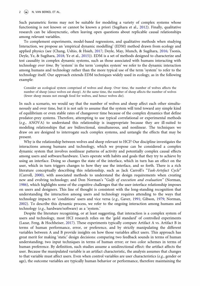
KEYWORDSUbicomp; mobile;performance; interaction;causality

1. Introduction

Human-Computer Interaction (HCI) research seeks to understand the causal interactions betweenusers and technology, ultimately leading to the design of improved interactive technology. To studycausal interactions, HCI researchers typically adopt one of three dominant approaches. The first isexperimental in nature, wherein researchers introduce participants to two or more conditions andcompare their effects on a variable of interest. The second relies on observational data and takesa model-based approach to estimate causal effects with regressions. For example, researchers maycollect contextual data and model the effect of these variables on device usage. The third approach isqualitative, collecting rich descriptions of ongoing user activity and experience within an experi-mental or observational study to understand dynamic interactions. Although these approaches canbe very useful, they have limitations. On the one hand, controlled experiments offer a simplifiedversion of reality, which limits the generalizability of results in real-world settings. On the otherhand, parametric modeling approaches rely on pre-determined equations that can be understood ashypotheses or assumptions about the structural relationships that define a system being modeled.

CONTACT Niels van Berkel [email protected] Aalborg University, Department of Computer Science, Denmark,9220 Aalborg Ø, DK, Selma Lagerløfs Vej 300© 2020 Taylor & Francis Group, LLC

HUMAN–COMPUTER INTERACTIONhttps://doi.org/10.1080/07370024.2020.1715221

http://orcid.org/0000-0001-5106-7692

http://orcid.org/0000-0003-2804-6038

https://crossmark.crossref.org/dialog/?doi=10.1080/07370024.2020.1715221&domain=pdf&date_stamp=2020-01-30

Such parametric forms may not be suitable for modeling a variety of complex systems whosefunctioning is not known or cannot be known a priori (Sugihara et al., 2012). Finally, qualitativeresearch can be idiosyncratic, often leaving open questions about replicable causal relationshipsamong relevant variables.

To complement experiments, model-based regressions, and qualitative methods when studyingInteraction, we propose an ‘empirical dynamic modelling’ (EDM) method drawn from ecology andapplied physics (see (Chang, Ushio, & Hsieh, 2017; Deyle, May, Munch, & Sugihara, 2016; Tsonis,Deyle, Ye, & Sugihara, 2018; Ye et al., 2015)). EDM is a set of methods designed to characterize andtest causality in complex dynamic systems, such as those associated with humans interacting withtechnology over time. By ‘system’ in the term ‘complex system’ we refer to the dynamic interactionamong humans and technology rather than the more typical use of the term ‘system’ to refer to thetechnology itself. Our approach extends EDM techniques widely used in ecology, as in the followingexample:

Consider an ecological system comprised of wolves and sheep. Over time, the number of wolves affects thenumber of sheep (since wolves eat sheep). At the same time, the number of sheep affects the number of wolves(fewer sheep means not enough food for wolves, and hence wolves die).

In such a scenario, we would say that the number of wolves and sheep affect each other simulta-neously and over time, but it is not safe to assume that the system will tend toward any simple kindof equilibrium or even stable rates of changeover time because of the complex dynamics that definepredator-prey systems. Therefore, attempting to use typical correlational or experimental methods(e.g., ANOVA) to understand this relationship is inappropriate because they are ill-suited tomodeling relationships that are bidirectional, simultaneous, and nonlinear. The techniques wedraw on are designed to interrogate such complex systems, and untangle the effects that may bepresent.

Why is the relationship between wolves and sheep relevant to HCI? Our discipline investigates theinteractions among humans and technology, which we propose can be considered a complexdynamic system that involves nonlinear patterns of activity and potentially complex causal effectsamong users and software/hardware. Users operate with habits and goals that they try to achieve byusing an interface. Doing so changes the state of the interface, which in turn has an effect on theuser, which in turn triggers changes to how they use the interface, and so forth. There is a richliterature conceptually describing this relationship, such as Jack Carroll’s “Task-Artefact Cycle”(Carroll, 2000), with associated methods to understand the design requirements when creatingnew and evolving technology; and Don Norman’s “Gulfs of execution and evaluation” (Norman,1986), which highlights some of the cognitive challenges that the user-interface relationship imposeson users and designers. This line of thought is consistent with the long-standing recognition thatunderstanding the interaction among users and technology requires attending to the ways thattechnology impacts or ‘conditions’ users and vice versa (e.g., Gaver, 1991; Gibson, 1979; Norman,2002). To describe this dynamic process, we refer to the ongoing interaction among humans andtechnology (e.g., hardware/software) as a ‘system.’

Despite the literature recognizing, or at least suggesting, that interaction is a complex system ofusers and technology, most HCI research relies on the ‘gold standard’ of controlled experiments(Lazar, Feng, & Hochheiser, 2017). These experiments typically compare Artifact A vs. Artifact B interms of human performance, error, or preference, and by strictly manipulating the differentvariables between A and B provide insights on how those variables affect users. This approach hasgreat merit for making ‘static’ design decisions: comparing two feedback sounds in terms of humanunderstanding; two input techniques in terms of human error; or two color schemes in terms ofhuman preference. By definition, such studies assume a unidirectional effect: the artifact affects theuser. Because the manipulated variable is an artifact characteristic, the analysis assumes that changesto that variable must affect users. Even when control variables are user characteristics (e.g., gender orage), the outcome variables are typically human behavior or performance, therefore maintaining the

2 N. VAN BERKEL ET AL.

unidirectional-effect assumption. However, simply because manipulations and measured outcomevariables are restricted to specific factors does not mean that causality is unidirectional. Instead, itimplies a potential shortcoming of experimental methods wherein researchers assume unidirectionalcausality and incorporate this assumption into a study through its design, thus offering a partialpicture of a potentially complex system.

Alternatively, ‘dynamic’ longitudinal studies (such as ‘in-the-wild’ studies) provide a more realis-tic setting for observations, often going beyond more simplistic and unidirectional approaches tounderstanding the complex relationship between people and technology. Researchers who try tomake sense of longitudinal in-the-wild data typically approach analysis with two broad strategies.One relies on regression to estimate the effects of multiple variables on an outcome of interest.A second approach is a field experiment with efforts to randomize conditions and analyses that testdifferences between them. Unfortunately, both approaches may fail to characterize the complexdynamic relationship among users and technology – neither regression models nor field studies andtheir analyses can entirely capture the complexity of a complex system and the potentially bidirec-tional effects involved in real-world interactions among users and technology. On the one hand,regression models would need to be parameterized properly to estimate the effects of interest, but ifa system is complex it will be unreasonable to expect researchers to know these parameters a priori.On the other hand, field experiments often suffer from the same problems as typical lab experimentsmentioned previously. Of course, qualitative analyses using grounded theory and other approachescan address such shortcomings, but as we noted they have their own drawbacks including theidiosyncratic nature of the results, making it difficult to precisely evaluate and generalize causaleffects of interest.

To overcome some of these limitations, in what follows we present a novel method for analyzinglongitudinal human performance and artifact states using time-series data. As the system definingtheir interaction changes over time (i.e., as the states of the system change) in potentially nonlinearand causal ways, our proposed approach is designed to characterize the system and test causality init – ideally suited for highly granular (i.e., many observations over a period of time) datasets. Ourmethod extends a technique known as convergent cross mapping (CCM) that distinguishes causa-tion from correlation, which was published recently in Science (Sugihara et al., 2012). This techniqueis a core component of the EDM approach that we describe and exemplify. Our paper makesa number of contributions:

● First, as a tutorial, we tease apart the nuances of modeling interactions in a complex system,and describe how complex dynamic system methods can be used within HCI. In what follows,we do so by initially elaborating on our points about more traditional HCI methods, experi-mental and observational studies, and then proceed to discuss EDM and its logic.

● Second, methodologically, we develop a novel way of combining, visualizing, and evaluatingEDM results for multiple individuals in a sample. This has been a limitation of existingmethods, which typically focus on a single entity (e.g., a single ecosystem), or treat multipleentities as if they were homogenously defined by a single dynamic system (e.g., Clark et al.,2015). We call our alternative approach Multiple Convergent Cross Mapping (MCCM), whichtreats each entity as a potentially unique dynamic system. We publicly release our analysis codeto support the wider community in assessing and adopting MCCM.1

● Third, as a case study, we apply our method in the context of HCI by analyzing userinteractions on mobile devices through multiple datasets, demonstrating how our analysisenables researchers to establish the causal direction and distance between two variables ofinterest. As part of exemplifying our method, we answer questions (amongst others) such as: dopeople tend to use their phones because they receive notifications, or do they receive notifica-tions because they use their phones, or both (i.e., bidirectional causality)? We also elaborate on

1https://github.com/nielsvanberkel/Multiple-Convergent-Cross-Mapping.

HUMAN–COMPUTER INTERACTION 3

https://github.com/nielsvanberkel/Multiple-Convergent-Cross-Mapping

the “so what” of these results by describing how they can be understood in a practical sense forinference and design.

● Fourth, we conclude with thoughts on wider applications of EDM for the HCI community, aswell as advances to EDM that will aid HCI researcher’s in their question to better understandand model causal effects in the complex dynamic systems that define humans and theirinteraction with technology.

2. Related work

2.1. Correlation vs. causation in HCI

In their book ‘Research Methods in Human-Computer Interaction,’ Lazar et al. highlight that “one ofthe most common objectives for HCI-related studies is to identify relationships between various factors”(Lazar et al., 2017). Qualitative methods identify such relationships by identifying and linkingthemes and codes as discerned through an interview or observational data. Grounded theory, inparticular, has a strong focus on identifying causal relationships (Charmaz, 2006), for example,through axial coding (Corbin & Strauss, 2008). Quantitative HCI studies of human participants aretypically experimental or observational in nature. These approaches typically have the followingcharacteristics (which may also include qualitative components):

● Experimental study: the researcher intervenes in the reality of participants (e.g., by introducingstudy conditions) and measures the effect of these interventions (Figure 1a). Such studies areoften, but not necessarily, conducted in a laboratory environment, which allows control overpotential confounds. However, in such studies the lack of a real-world context can reduce thegeneralizability of study results (Dix, Finlay, Abowd, & Beale, 2003). Additionally, one keyelement of control that underpins the ability of experimental approaches to determine causalityis random and/or counterbalanced conditions for participants, which can bias or interact withthe relationships among causal variables.

● Observational study: the researcher does not intervene in the reality of the participants, butinstead attempts to understand the interplay between the artifact and user, typically by

Figure 1. Illustration of two commonly used research approaches in HCI. (a) Experimental study, in which the effect of differentconditions is assessed. (b) Observational study, in which the interplay between artifact and user is more often assessed.


observing variables of interest over time (Figure 1b). These studies are usually conducted in-the-wild rather than in a lab, and allow the researcher to observe the user, as well as theirinteraction with a potential artifact, in their natural environment. As the researcher does notintervene in the reality of the participants, no conditions (i.e., manipulations) are introduced toparticipants. In such cases, it is important for the researcher to be able to distinguish betweennaturally occurring correlational versus causal relationships among variables.

The primary purpose of experiments and observational studies is to help researchers estimate andinfer causal effects – although more exploratory approaches can also be used these are less commonand are not our focus here. Consistent with the well-known dictum that ‘correlation does not implycausation,’ the problem is that many observed associations among variables cannot simply beunderstood as causal. In our example, researchers may find a relationship between mobile notifica-tions and smartphone usage, but then not know if both variables have common causes, one causesthe other, or bidirectional causality exists.

Untangling correlation and causation is a topic that has recently received increased attentionacross multiple disciplines, including HCI. To address it, researchers have taken various experi-mental and observational approaches, such as Tsapeli et al. (Tsapeli & Musolesi, 2015) and Mehrotraet al. (Mehrotra, Tsapeli, Hendley, & Musolesi, 2017) in their analysis of the relationship betweensmartphone interaction and the emotional state of the user. Their findings indicate that the emotionsof the smartphone user have a causal impact on different aspects of smartphone interaction. In theirwork, Mehrotra et al. (Mehrotra et al., 2017) first perform a correlation analysis to determine whichvariables have a significant relationship. For example, one of the tested correlations is the user’s self-reported stress level and a number of received notifications. Following this, the variables which aresignificantly correlated (α < 0.05) are tested for causality using a matching design framework asintroduced in (Lu, Zanutto, Hornik, & Rosenbaum, 2001). In this approach, a pair of two variables istested for causality and an ‘average treatment effect’ is calculated by taking into account a set of pre-selected confounding variables (Tsapeli, Musolesi, & Tino, 2017). The average treatment effectindicates the direction of the causation and includes an indicator of significance.

Such approaches rely on some form of regression in an attempt to mimic experiments. Forexample, instances of users exhibiting behavior A are matched to instances of users exhibitingbehavior B under the same circumstances. Although the goal of establishing causality in this wayis important, such methods are problematic when dealing with complex systems for at least tworeasons: 1) when variables are deterministically related in a system, then controlling for any onevariable can eliminate important aspects of overall system dynamics; and 2) assuming how variablesare related to each other is required a priori to construct a parametric model that will have theassumptions embedded in it, such as when researchers first check for significant bivariate correla-tions, which can be zero even though causal relationships exist that are nonlinear in nature (Sugiharaet al., 2012).

Indeed, although researchers are well aware that two variables may be correlated but lack a causalrelationship, they typically overlook the inverse fact: two variables may be uncorrelated but can stillbe causally related because they are a function of complex system dynamics that are nonlinear. Thisfact undermines both experimental and observational approaches that usually rely on linear covar-iance analysis, and thus even observational methods that are designed to mimic an experiment arenot necessarily well suited for studying complex dynamic systems, which we now discuss.

2.2. Complex dynamic systems and EDM

Complex dynamic systems consist of multiple interacting components that produce inherentlyunstable and nonlinear behavior as a system evolves over time, such as the interaction betweenusers and technology evolving dynamically over time. This evolution occurs in state-dependent ways,meaning the way a system functions depends on its current and historical states, such as a user’s next


actions or a technology’s next alerts depending on the recent past. Complex dynamic systems can befound all around us, and as such the idea of dynamic systems has been applied to a wide variety ofdisciplines with phenomena that can be described using a small number of variables/dimensionsbehaving nonlinearly (Larsen-Freeman, 2015), including the spread of diseases (Galea, Riddle, &Kaplan, 2010), ecological diversity (Carpenter & Brock, 2006), financial markets (Mauboussin, 2002),and human development (Dörnyei, Henry, & MacIntyre, 2014). Dynamic systems evolve based onthe interaction of the components in the system, with the goal of the researcher often being topredict or forecast the next state of the system based on recent states. Given the complexity and non-linearity of dynamic systems, the use of linear statistical methods (common in experimental andobservational designs) is not suitable: “Linear approaches are fundamentally based on correlation.Thus, they are ill-posed for dynamical systems, where correlation can occur without causation, andcausation may also occur in the absence of correlation” (Chang et al., 2017).

Empirical dynamic modeling or EDM is a non-linear approach to studying dynamic systemsbased on Takens’s theorem (Takens, 1981), which describes how the behavior of a multi-variablecomplex system can be reconstructed based on a time series of a single variable, as can be seen in thevideo2 included in (Sugihara et al., 2012). The crucial insight in Takens’s theorem is that all therichness and diverse behavior of a complex system can be reconstructed by analyzing any singlevariable that is associated with the system. This theorem is important for HCI studies, because eventhough there may be confounding variables that a study has not captured, Takens’s theorem suggeststhat those confounding variables nevertheless leave an imprint on the variables that are measured. Assuch, we can reconstruct the behavior of an entire system by capturing just a single variable. Thus,traditional concerns about confounds are fundamentally altered and potentially alleviated becausethe traditional approach of attempting to control for relevant system variables can actually make itmore difficult to reconstruct the dynamical behavior of a system – controlling for any variablesrelevant to a system can eliminate important system dynamics – thus making the results from typicalregression models potentially suspect.

Based on Takens’s theorem, EDM operates with minimal assumptions about the exact nature ofa dynamic system by using a time-series to reconstruct the system’s behavior, thus making it“suitable for studying systems that exhibit non-equilibrium dynamics and nonlinear state-dependentbehavior” (Ye et al., 2019). This is done in a three-step process:

(1) the dimensionality E of a dynamical system is assessed using a method known as simplexprojection, and we continue to the next step if E is sufficiently low (<15 in our case);

(2) using a method known as S-mapping, we assess whether the system evolves nonlinearly (i.e.,in state-dependent ways); and then

(3) based on results from the previous analyses, convergent cross mapping or CCM is used toassess causal relationships among variables that define a dynamical system (see (Sugiharaet al., 2012)), and then practical implications and design inferences are drawn based onresults. This third step is important because, for example, variables in dynamic systems candisplay a positive correlation at some times, while displaying no correlation or evena negative correlation at other times (Sugihara et al., 2012) – a phenomenon known as‘mirage correlation.’ Thus, linear analysis methods may misconstrue and fail to uncovera large number of nonlinear behaviors and causal effects due to the nonlinearity of variablesin dynamic systems, leading to inferences and design decisions that may be suboptimal.CCM helps overcome this potential problem by assessing causal effects without linearassumptions.

In contrast to predictions based on a predefined set of equations as in typical regression models,“EDM […] relies on time series data to reveal the dynamic relationships among variables as they

2https://www.youtube.com/watch?v=6i57udsPKms.


https://www.youtube.com/watch?v=6i57udsPKms

occur” (Ye et al., 2015). This dynamic relationship among variables, wherein correlations depend onthe state of a system, is a typical aspect of complex nonlinear systems. EDM was originally applied toecosystem forecasting (Ye et al., 2015), where it outperforms traditional modeling methods bymaking highly accurate forecasts – allowing better fisheries management, for example. EDM isnow being applied in a wide range of disciplines with similar benefits, including finance, neu-roscience, and genetics (Popkin, 2015). These fields typically produce a large amount of longitudinaldata where the interest is in using observed variables to make causal inferences. Based on this path-breaking work, we argue that EDM and CCM can be helpful in analyzing human-technologyinteraction data in HCI studies, especially under conditions that share these characteristics ofdynamic systems.

Specifically, inspired by Jack Carroll’s (Carroll, 2000), Don Norman’s (Norman, 1986), andWilliam Gaver’s (Gaver, 1991) work, we argue that human-technology interaction bears the hall-marks of an evolving complex dynamic system. Technology use is often non-linear and episodic, asshown by a wide range of studies on technology interaction (e.g., learning effect, technologicaladoption). Furthermore, our relationship with technology is bidirectional (e.g., a person’s interest insocial media causally drives smartphone use, and increased smartphone use can lead to the increasedtime spent on social media). Finally, our interaction with technology is driven by many factors (e.g.,friends, weather, trends), which can dynamically change both by themselves and in relation to oneanother in nonlinear ways. By definition, it is impossible to account for all of these (confounding)factors in typical linear models. As such, we propose to model the interaction between humans andtechnology as a dynamic system in order to gain further insights into how such systems function,including causal effects among the variables that define them.

Although a limited number of researchers have attempted to separate correlation and causality inthe domain of HCI, their approaches typically concern linear systems which are unable to accountfor the complex patterns of technology use. Although EDM has great potential for fields such as HCIthat involve the study of complex dynamic systems, to our knowledge no paper has described the useof EDM in HCI literature.

2.3. Our methodological contribution

Previous work has been highly successful in applying the concept of complex systems to studysingular entities (e.g., an individual rainforest or a single stock market). Although these analyses havetraditionally focused on ecosystems (Sugihara et al., 2012; Ye et al., 2015), recent work has alsobegun to investigate individual human behavior. All aforementioned studies, however, are limited tothe analysis of an individual system. This works well in the analysis of ecosystems, wherea researcher tries to understand the dynamics of a single ecosystem, or a single financial market.However, this approach will not transfer well to HCI when multiple users are studied and each one istreated as an independent ecosystem.

For example, while different groups of shoaling fish can ultimately be considered as functioningwith common rules that define a common dynamic system, the same may not apply to a group ofstudy participants, each of which may function according to unique rules that define a uniquedynamic system. Participants in a typical HCI study may be unique in important ways, utilizingpersonal devices in potentially different ways in different contexts, rather than sharing technologicaland behavioral interactions in a common environment. Furthermore, consistent with the notion ofa complex dynamic system, we expect that even with very similar starting conditions (e.g., a newsmart-phone with a single set of default settings), differences will emerge over time betweenparticipants in the ways that they interact with technology. Therefore, analyzing the data frommultiple participants as if they originate from a single ecosystem may mask the uniqueness ofinteractions that define each individual and their technology. In sum, EDM can be used to analyzedata from one entity or multiple entities (see e.g. (Clark et al., 2015)), but heretofore this has oftenbeen done by treating the behavior of the entities as being part of a single dynamic system. In what


follows, we extend EDM to the case of multiple users who may not share a common dynamic system,and we present a novel way to summarize and validate the multiple independent analyses associatedwith this case. We call this approach multiple convergent cross mapping or MCCM, which estimatesunique causal effects for each system/participant sampled over time. In what follows, we describe thelogic of EDM, CCM, and then MCCM through a real-world illustration.

3. Method and results

3.1. Datasets

We exemplify our method by applying it to multiple independent datasets – each with multiple usersand, thus, multiple unique dynamic systems. Our purpose is to identify and characterize relation-ships for a range of variables associated with mobile device use, specifically by: 1) characterizing thedynamical system associated with each user’s data using simplex projection and S-mapping as notedpreviously, and then; 2) with results from this step use CCM to assess causal effects among variablesof interest.

Dataset 1 consists of smartphone use traces from 20 participants collected during a 3-week in-the-wild study (van Berkel et al., 2018). Participants were recruited from a university campus usingmailing lists and had a diverse educational background. A mobile application was installed onparticipants’ phones, and ran continuously in the devices’ backgrounds. Participants used theirpersonal phones in order to ensure realistic usage behavior. During the study, participants wereasked to complete up to six questionnaires per day using the Experience Sampling Method (ESM).The study’s goal was to capture the effect of different ESM notification scheduling techniques onparticipant response rate and accuracy. The application collected, inter alia, device ID, phone usage,battery level, and application usage data. The data were cleaned by removing applications initiated bythe operating system (e.g., application launcher, keyboard). Following this, the dataset containedover 78,500 application usage events, over 137,000 notification events, and close to 3 million batteryevents (i.e., changes in battery level or charging status).

Dataset 2 is an extension of the dataset of the study reported in (Visuri et al., 2017). It consists ofsmartwatch use traces of 589 smartwatch users, collected between January 2016 and February 2017.67.9% of the users (N = 400) had the application installed and logging for less than 30 days (M =7.49, median = 5), 17.7% of the users (N = 104) for a timespan between 30 and 90 days (M = 54.66,median = 52), and 14.4% of the users (N = 85) for more than 90 days (M = 178.36, median = 148).Objective of the data collection was to obtain a better understanding of the interaction between usersand their smartwatch. Data collected by the application which are of relevance here are device ID,smartwatch screen events (turned on, turned off), and notification information (time and applica-tion). The total dataset consists of 6.1 million notifications and 2.0 million screen usage events.

Dataset 3 contains data from a laboratory experiment (Sarsenbayeva et al., 2017), wherebyparticipants’ finger temperature was recorded while using a smartphone. The sample contains 24participants, each of whom spent approximately 90 min completing tasks on a smartphone. Two ofthe experimental conditions took place in a cold chamber with a temperature of −10°C, whereas theremaining two conditions took place in room temperature. During the study, the thumb and indexfinger temperature of the participants were recorded continuously. In addition, the temperature ofthe smartphone battery was collected continuously. The study aimed to quantify the effect of coldtemperature on participant interaction with a smartphone.

For datasets 1 and 2 we calculate an hourly metric per measurement variable for each participant,and for battery data we calculate the average battery percentage per hour. Phone usage is calculatedas the number of times the phone was turned on per hour. For the remaining variables (applicationusage and incoming notifications) we count the total number of events per hour. For Dataset 3, weconsider each experimental task as the unit of analysis. For each task (which lasted a few seconds) wecalculate both the average temperature of the participant’s active finger (thumb or index depending


on how the phone was held) and the average battery temperature during that period. The partici-pants from all three datasets are unique.

3.2. Method

To conduct analyses we use the R package ‘rEMD’ by Ye et al. (Ye et al., 2019). We now describe thesix steps of our method, adapted from (Ye et al., 2019), including the process of data wrangling,MCCM, and a final robustness check. We develop this process in order to highlight the differences/similarities between participants in a study We apply this method to the aforementioned datasets inthe subsequent section.

Data treatmentEDM requires data in a typical time-series or panel data format (i.e., a ‘long’ format where eachoccasion of measurement is a row and variables are columns; see Table 1). For Datasets 1 and 2 weformed a time series consisting of 24 hourly entries per day. For Dataset 3 the time series consists ofthe experimental tasks, each of which lasted a few seconds. If the variable of interest did not occur ina specific-time period (e.g., a participant did not receive a notification during a given hour), weassigned a value of 0 for that time period. If a participant has insufficient data available for analysis(i.e., limited number of rows), the participant was completely discarded. In our case, we discardparticipants with less than 10 data points. Using this cutoff point, we discard zero participants fromDataset 1, 30 participants from Dataset 2, and zero participants from Dataset 3. The minimumnumber of data points is dependent on the study design and research questions.

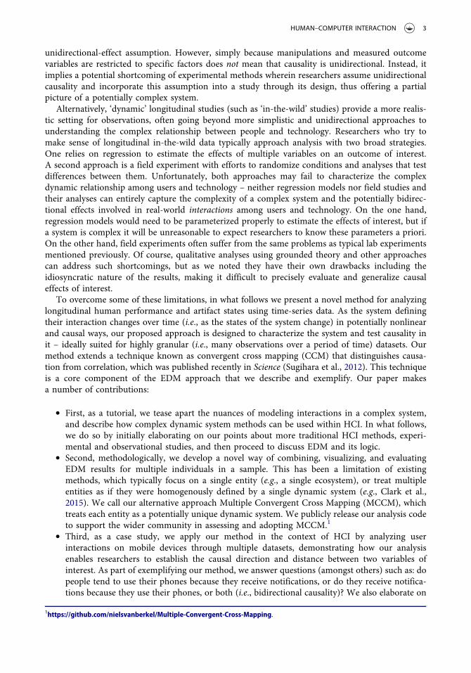
Identify the optimum value for E (Embedding Dimension)In this step, we identify the optimum embedding dimension (E) using simplex projection, asrecommended for EDM (Ye et al., 2019). The method uses time-delay embedding on a singlevariable to generate a complex system reconstruction, and then applies the simplex projectionalgorithm to make forecasts. In brief, consistent with Takens’s theorem, the idea is to use a set ofE lagged values of a variable to reconstruct the behavior of a dynamic system in E-space. Each pointin E-space is formed using E lags of a variable, and these points form an ‘attractor’ or an ‘attractormanifold’ that defines system evolution (e.g., a classic example of the Lorenz or ‘butterfly’ attractor).Then, for a given point on the manifold, the quality of the reconstruction is evaluated by finding theE + 1 ‘nearest neighbour’ points on the manifold, and then projecting these neighbors into the future

Table 1. Example slice from collected data.

Row # Participant ID Date Hour Notifications

171 4939097448 01-01-2018 14 12172 4939097448 01-01-2018 15 0173 4939097448 01-01-2018 16 8

Figure 2. Three steps in calculating an empirical dynamic model. (a & b) Identify optimum values for E for both variables. (c & d)Verify non-linearity for both variables. (e) Convergent cross mapping.


to make predictions. This forecast ability is calculated as the correlation between the observed andpredicted values – we annotate this value as ‘rho’ ρ. For different values of E, we plot the forecastskill as the correlation ρ among predicted and observed future values in a hold-out subsample(Figure 2a and b). We select the value of E that maximizes this correlation. The optimum value ofE provides the best out-of-sample predictions of the future, implying that an underlying dynamicalsystem has been optimally reconstructed. The identified optimum E value is then used to furtheranalyze each variable for each participant. Furthermore, the functional form of the E-ρ relationshipis useful for diagnosing the nature of a system. Low-dimensional deterministic systems with lownoise will have ρ maximized at a large value (i.e., close 1) when E is small (in our case less than 15).Alternatively, high-dimensional deterministic systems or stochastic systems with autocorrelation willtypically show ρ increasing with E, and potentially stabilizing rather than falling at very largeE (Sugihara, 1994).

Test for nonlinearityCCM is a nonlinear analysis technique, and it is, therefore, useful to check whether a system evolvesin a nonlinear fashion rather than merely being defined by linear autocorrelated noise. rEMD usesS-maps (Sugihara, 1994) to distinguish between Brownian noise (also known as ‘red noise’) andnonlinear deterministic behavior (Ye et al., 2019). In brief, this is done by using the E chosen fromthe previous step of simplex projection, and then estimating a linear map that uses theE-dimensional points on a manifold’s surface to predict the future. As done for rEDM, we define‘theta’ as the S-map tuning parameter which adjusts the sensitivity to nearby versus distant points forthe mapping. When theta = 0, all points on the manifold are equally weighted and therefore the mapreduces to a kind of autoregression, but when theta >0 the map is more sensitive to nearby pointsand thus the mapping is more local and, therefore, state-dependent. As can been seen from Figure 2cand d, if in the produced graph the forecast ability is greatest when theta = 0, then this means thedata can be modeled by an autoregressive model. If the prediction is greatest when theta > 0, thenmore local information is more useful for prediction of the future, implying state-dependent systemevolution and therefore a nonlinear process. We explicitly label as “invalid” participants whose datais auto-correlated, and assign theta = 0. In our case, this tends to happen due to a small dataset, ora dataset with non-rich data. This is critical, as even a purely stochastic (i.e., random) time seriesmay show predictability as the result of linear autocorrelation. Using the aforementioned approach,we are able to distinguish between autocorrelation and nonlinearity.

Convergent cross mapping for each userThe next step is to apply CCM to identify a potential causal link between the variables for each user.CCM is specifically developed for analyzing causality in time series variables (Sugihara et al., 2012).In brief, the method works by mapping two variables to each other using the nearest neighbors ofeach point on the E-dimensional manifolds. When the number of points on the manifold or the‘library’ size L increases, the nearest neighbors tend to become nearer, which improves predictions ifthe variables are causally linked (i.e., more local information improves prediction if the variables arecausally linked). This improvement is called convergence. The results of CCM are displayed inFigure 2e. We must apply a number of heuristics when interpreting these results for each user. First,we look for a clear convergence of the CCM value, i.e., verifying that the blue and red solid lines areinitially increasing and then eventually level-off. We also decided to apply an asymptote function toidentify a single point on the y-axis where we assume each series converges. Next, we compare thetwo asymptotes and determine which one is the largest (i.e., which one is on top). Finally, we checkto see if the asymptote that is on top is also above the bivariate correlation among the variables(indicated with a black dashed line). This correlation value is calculated as a straightforward Pearsoncorrelation between the two variables of interest.


Combine the results from multiple analysesThis step represents our extension to the CCM technique, which we developed to summarize theresults from multiple CCM analyses, hence the acronym MCCM. We developed this step with theobjective of obtaining a rich summary of the similarities and differences between large numbers ofparticipants. Our objective was to generate a single graph to summarize a large number of analyses.After trying a number of visual approaches, we settled on the following approach which highlightsdifferences between participants: For each analysis (i.e., participant) we plot the difference inasymptotes (the relative difference indicates the direction of the effect) versus the difference of thelargest asymptote and the correlation value (indicating the effect size), as calculated between the twovariables. We finally calculate the mean value for the direction of the effect across all studyparticipants in order to summarize effects among the variables for the entire sample (the standarddeviation can also be used to assess dispersion if the effect distributions are approximately normal).This enables a kind of dominance analysis that allows inferring which direction of effect appears tobe strongest for two variables.

Robustness checkThe final step is to determine the robustness of the findings. We do so by adopting a “proxy data”approach. Here, we compare our findings against a null model obtained by random permutations ofthe raw data – also known as a ‘surrogate data’ method in the EDM literature.

In the figure below, we summarize our analysis for a single participant in the smartphone dataset.Here we seek to understand the effect of two variables on each other: the number of times theparticipant turned on the phone by pressing the unlock button (“screen_on”), and the number ofnotifications that the phone received. The variables were coded as we described earlier, and thereforeare counted on an hourly basis. In Figure 2a and b we identify that the optimum E for thisparticipant’s data is 11 and 30, respectively. In Figure 2c and d we verify that the data is nonlinear(since the maximum forecasts skill is at ~2.0 and ~1.8, which are greater than 0). Finally, in Figure 2ewe observe that, for this participant, the number of times they unlock the screen is more likely todrive the number of notifications they receive (rho = 0.5) rather than the other way around (rho =0.17). This is because the red line reaches a higher convergence point than the blue line.Furthermore, we observe that this is a substantial finding since the red line converges at 0.5 whichis much larger than the raw bivariate correlation between these two variables (r = 0.21, shown inblack dashed line). Although convergence in CCM is the primary arbiter for causal inference, ourapproach allows straightforward inferences regarding which of two variables appear to have thestronger effect on the other. Based on these results, we can draw various practical conclusions suchas what drives someone’s use of a technology, the effect of external influencers (e.g., notifications) onuser behavior, or identify clusters of different influencers among a user group. This newfoundknowledge on the drivers behind certain usage patterns can inform the design of technology byincreasing or decreasing these drivers accordingly.

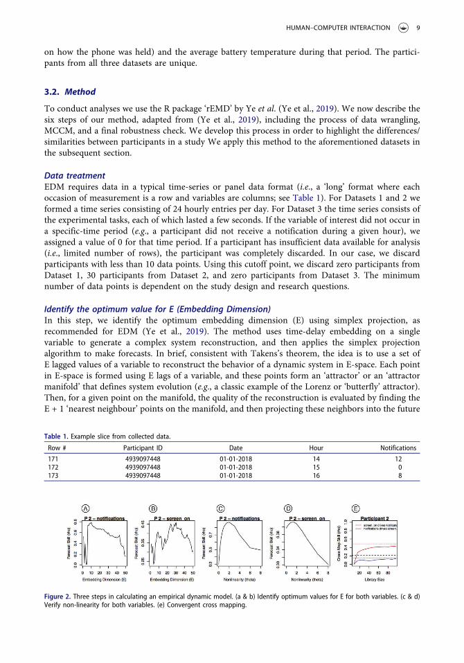
In Figure 3 we provide examples where the data fail our heuristics and we decide to discard theparticipant from the analysis. In Figure 3a we show data from a participant whose data does notappear to be non-linear. In Figure 3b we show data from a participant where our analysis does notprovide significant results since the highest asymptote (red-dashed line in this case) is below thecorrelation line (black-dashed line). Finally, in Figure 3c we show the results from a user where theCCM results do not converge (i.e., the top-red line appears to be flat) and thus causal effects cannotbe inferred.

The process we have described in Figure 2 is what would be followed to analyze a single complexdynamic system, e.g., studying the relationship between the number of toads and snakes in theamazon rainforest. We apply our method to each participant independently, and therefore ouranalysis produces one graph per participant (as shown in Figure 2e), which with even a modestsample size can be cumbersome. Therefore, we need to extend this method and developa meaningful way to summarize results for all participants, and draw conclusions about the variables


we are analyzing for an entire sample of people. For example, this would be equivalent to studyingthe relationship between toads and snakes across N different rainforests. In our case, we may getconflicting results from different participants, and different effect sizes, and therefore it is necessaryto arrive at a conclusion that moves beyond simply eyeballing the hundreds of graphs we and othersmight generate.

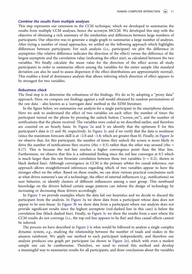
To summarize the results from multiple participants, we adopt a geometric approach. In Figure 4we visualize how we can summarize the CCM results from multiple participants, or multipleecosystems. Looking at the CCM results of each participant, we first calculate two values:

● the difference between the two asymptotes. This is the vertical difference between the red-dashed line and the blue-dashed line, and is an indicator of the primary direction of an effect.

● the difference to the raw correlation. This is always calculated as the difference from the topasymptote (in this case the red-dashed line) to the correlation (the black-dashed line). This isan indicator of the strength of the effect to the extent that CCM reflects nonlinear dynamicsthat are not reflected in linear bivariate correlations.

Having calculated these two values, we use them as the x and y coordinates, respectively, ina scatterplot, wherein we simply add a dot at those coordinates in the scatterplot. In the example inFigure 4 the difference between asymptotes is about −0.23, while the difference to the correlation isabout 0.1. Therefore, we add a datapoint at coordinates (−0.23, 0.1) in the scatterplot. In thisscatterplot, we use red to denote any data points (i.e., CCM graphs) that are to be discarded becausethey fail our heuristics.

Next, we calculate the mean x-axis value for all data points that we retain in the scatterplot. This isindicated as the thin vertical-dotted line at x = −0.192. This mean value is calculated using only theretained data points, ignoring the discarded data points. This value, along with the standard

Figure 3. Examples where a participant’s data must be discarded as it fails the heuristics of the analysis. 3A: The data fails the non-linearity test. 3B: The CCM results are not significant: they are below the correlation value. 3C: the CCM results do not converge.

Figure 4. A visualization of our geometric approach to summarizing CCM results for multiple participants. For each participant wecalculate the difference between asymptotes and the difference to correlation. These two values become the (x,y) coordinates ofa data in our summary scatterplot. All retained values are used to calculate the x-axis mean, as a means to summarize the overalloutcome of the analysis.


deviation, is then used to characterize the population and therefore summarize all results for allparticipants.

As shown in the rightmost of Figure 4, all points below the horizontal axis are ignored using ourapproach, since these represent graphs where the top asymptote is below the correlation line.Additional points may also be ignored if they fail one of the other heuristics (failing the non-linearity test, or lack of convergence), and in our experience this tends to happen with small or non-rich datasets. Furthermore, any data points in the top-left of the scatterplot indicate that variable 1 isstronger, while points in the top-right indicate that variable 2 is stronger.

Finally, we use a method to validate our results that is common in the EDM community:comparing observed results to a null model. We generate null models with the use of “surrogatedata” (Small & Tse, 2003). Surrogates are created by randomly permuting the values of the originaltime series on a participant level – eliminating temporal dependencies while preserving the histo-gram of the original data. We expect that if our findings are simply due to broad statistical featuresof the data in our observations, then these random permutations will produce results that are similarto our actual results. If our actual results are demonstrably different than the random permutations,then we argue that this is evidence that there is something special about the order in which theevents took place, and therefore they capture the underlying dynamics of a complex system thatevolves over time.

To conduct this validity test, we run CCM on the surrogate data and subsequently store theasymptote differences (i.e., the x-axis coordinates in Figure 4). The generation of surrogate data andsubsequent CCM calculation is independently repeated 25 times per participant. All values arereordered pairwise, thereby maintaining the correlation between the two timeseries. We presenta visual comparison of the actual data versus the surrogate data (see Figure 5 for an example), andconsider if the mean asymptote difference that we report in the plots is likely to belong to thedistribution of values observed in the surrogate data. We do so by considering the median and 95%confidence interval of each distribution. As can been seen from Figure 5, the difference betweenasymptotes for the surrogate data is centered around zero. These results are substantially differentfrom the results obtained from our participant population (shown directly below). It must, therefore,be the temporal order of the data (as observed in the participant data but randomly permuted in thesurrogate data) which causes the difference between asymptotes.

3.3. Results

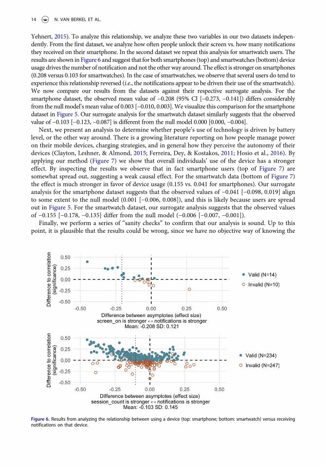
We now present the results of applying our method to investigate the relationship between a number ofvariables in our datasets. First, we investigate whether device use is driven by notifications, or the other wayaround. There is increasing literature suggesting that users have a hard timemanaging notifications on theirmobile devices, and that work has suggested that more notifications may be causing people to use theirdevice more often (Mehrotra, Pejovic, Vermeulen, Hendley, & Musolesi, 2016; Stothart, Mitchum, &

Figure 5. Comparison of CCM outcomes of surrogate data and participant data. If the two distributions are different then weexpect that our findings are not due to chance.


Yehnert, 2015). To analyze this relationship, we analyze these two variables in our two datasets indepen-dently. From the first dataset, we analyze how often people unlock their screen vs. how many notificationsthey received on their smartphone. In the second dataset we repeat this analysis for smartwatch users. Theresults are shown inFigure 6 and suggest that for both smartphones (top) and smartwatches (bottom)deviceusage drives the number of notification andnot the otherway around. The effect is stronger on smartphones(0.208 versus 0.103 for smartwatches). In the case of smartwatches, we observe that several users do tend toexperience this relationship reversed (i.e., the notifications appear to be driven their use of the smartwatch).We now compare our results from the datasets against their respective surrogate analysis. For thesmartphone dataset, the observed mean value of −0.208 (95% CI [−0.273, −0.141]) differs considerablyfrom the nullmodel’smean value of 0.003 [−0.010, 0.003].We visualize this comparison for the smartphonedataset in Figure 5. Our surrogate analysis for the smartwatch dataset similarly suggests that the observedvalue of −0.103 [−0.123, −0.087] is different from the null model 0.000 [0.000, −0.004].

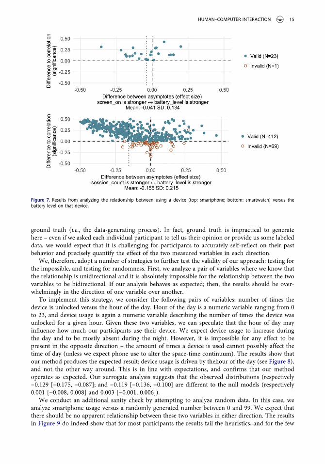
Next, we present an analysis to determine whether people’s use of technology is driven by batterylevel, or the other way around. There is a growing literature reporting on how people manage poweron their mobile devices, charging strategies, and in general how they perceive the autonomy of theirdevices (Clayton, Leshner, & Almond, 2015; Ferreira, Dey, & Kostakos, 2011; Hosio et al., 2016). Byapplying our method (Figure 7) we show that overall individuals’ use of the device has a strongereffect. By inspecting the results we observe that in fact smartphone users (top of Figure 7) aresomewhat spread out, suggesting a weak causal effect. For the smartwatch data (bottom of Figure 7)the effect is much stronger in favor of device usage (0.155 vs. 0.041 for smartphones). Our surrogateanalysis for the smartphone dataset suggests that the observed values of −0.041 [−0.098, 0.019] alignto some extent to the null model (0.001 [−0.006, 0.008]), and this is likely because users are spreadout in Figure 5. For the smartwatch dataset, our surrogate analysis suggests that the observed valuesof −0.155 [−0.178, −0.135] differ from the null model (−0.006 [−0.007, −0.001]).

Finally, we perform a series of “sanity checks” to confirm that our analysis is sound. Up to thispoint, it is plausible that the results could be wrong, since we have no objective way of knowing the

Figure 6. Results from analyzing the relationship between using a device (top: smartphone; bottom: smartwatch) versus receivingnotifications on that device.


ground truth (i.e., the data-generating process). In fact, ground truth is impractical to generatehere – even if we asked each individual participant to tell us their opinion or provide us some labeleddata, we would expect that it is challenging for participants to accurately self-reflect on their pastbehavior and precisely quantify the effect of the two measured variables in each direction.

We, therefore, adopt a number of strategies to further test the validity of our approach: testing forthe impossible, and testing for randomness. First, we analyze a pair of variables where we know thatthe relationship is unidirectional and it is absolutely impossible for the relationship between the twovariables to be bidirectional. If our analysis behaves as expected; then, the results should be over-whelmingly in the direction of one variable over another.

To implement this strategy, we consider the following pairs of variables: number of times thedevice is unlocked versus the hour of the day. Hour of the day is a numeric variable ranging from 0to 23, and device usage is again a numeric variable describing the number of times the device wasunlocked for a given hour. Given these two variables, we can speculate that the hour of day mayinfluence how much our participants use their device. We expect device usage to increase duringthe day and to be mostly absent during the night. However, it is impossible for any effect to bepresent in the opposite direction – the amount of times a device is used cannot possibly affect thetime of day (unless we expect phone use to alter the space-time continuum). The results show thatour method produces the expected result: device usage is driven by thehour of the day (see Figure 8),and not the other way around. This is in line with expectations, and confirms that our methodoperates as expected. Our surrogate analysis suggests that the observed distributions (respectively−0.129 [−0.175, −0.087]; and −0.119 [−0.136, −0.100] are different to the null models (respectively0.001 [−0.008, 0.008] and 0.003 [−0.001, 0.006]).

We conduct an additional sanity check by attempting to analyze random data. In this case, weanalyze smartphone usage versus a randomly generated number between 0 and 99. We expect thatthere should be no apparent relationship between these two variables in either direction. The resultsin Figure 9 do indeed show that for most participants the results fail the heuristics, and for the few

Figure 7. Results from analyzing the relationship between using a device (top: smartphone; bottom: smartwatch) versus thebattery level on that device.


remaining participants the results are small and close to 0. This confirms our expectation that noapparent effect is observed. Our surrogate analysis suggests that the observed distribution (−0.002[−0.020, 0.027]) is very similar to the null model (−0.006 [−0.130, 0.001]).

Our next sanity test, and in many ways a prime demonstration of the benefits of our method,comes from analyzing data that are correlated but we know there is no causal effect between thesetwo variables. We created two variables (i.e., columns in a table) in the smartphone dataset, asfollows:

● random2: = 0.5*notifications + random1● random3: = 0.3*notifications + random1

Because of the way ‘random2ʹ and ‘random3ʹ are generated, they have a very high correlation (r =0.97); however, we know that they cannot cause each other because they are only directly affected by the

Figure 8. Results from analyzing the relationship between using a device (top: smartphone; bottom: smartwatch) versus the hourof day.

Figure 9. Results from analyzing the relationship between using a smartphone versus a random number.


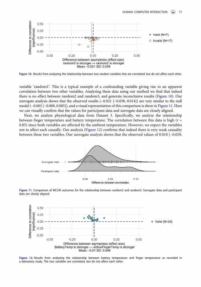
variable ‘random1ʹ. This is a typical example of a confounding variable giving rise to an apparentcorrelation between two other variables. Analyzing these data using our method we find that indeedthere is no effect between random2 and random3, and generate inconclusive results (Figure 10). Oursurrogate analysis shows that the observed results (−0.021 [−0.058, 0.014]) are very similar to the nullmodel (−0.003 [−0.009, 0.005]), and a visual representation of this comparison is show in Figure 11. Herewe can visually confirm that the values for participant data and surrogate data are closely aligned.

Next, we analyze physiological data from Dataset 3. Specifically, we analyze the relationshipbetween finger temperature and battery temperature. The correlation between this data is high (r =0.85) since both variables are affected by the ambient temperature. However, we expect the variablesnot to affect each causally. Our analysis (Figure 12) confirms that indeed there is very weak causalitybetween these two variables. Our surrogate analysis shows that the observed values of 0.010 [−0.029,

Figure 10. Results from analyzing the relationship between two random variables that are correlated, but do not affect each other.

Figure 11. Comparison of MCCM outcomes for the relationship between random2 and random3. Surrogate data and participantdata are closely aligned.

Figure 12. Results from analyzing the relationship between battery temperature and finger temperature as recorded ina laboratory study. The two variables are correlated, but do not affect each other.


0.007] are similar to the null model (−0.001 [−0.01, 0.008]). This case highlights an example wherethe data are nonlinear but not causally related.

Finally, we present a comparison between the aforementioned test results and their respectivesurrogate results in Figure 13, containing the asymptote differences for all original and surrogatedata. This overview visualizes the aforementioned mean values and confidence intervals, andprovides further evidence for our method of analysis. Tests which report no clear causality havea strong overlap with the causal data (e.g., tests with random data or the ‘BatteryTemp’ ↔‘ActiveFingerTemp’ test) – whereas test which report a strong causal relationship have no overlapwith the surrogate data. Close alignment with the surrogate data indicates that the order of the datais unable to reveal causal information on the variables of interest.

4. Discussion

HCI researchers have typically drawn on a variety of methods for analyzing their study results (Lazaret al., 2017). Even though the dictum ‘correlation does not imply causation’ is well known within ourdiscipline, only a handful of previous work has aimed to rigorously tease apart correlation andcausality. Here, we present a novel causality test from nonlinear dynamical systems analysis, apply itto multiple recent datasets, and develop a new way to interpret the results for multiple participants.

Although previous work has applied this method to singular entities (e.g., Cramer et al., 2016;Sugihara et al., 2012; Ye et al., 2015), HCI researchers typically analyze larger groups of participantsrather than individual entities. Our proposed method of analysis differs from the existing work inHCI on identifying causal relationships (e.g., Mehrotra et al., 2017; Tsapeli & Musolesi, 2015). First,our approach does not use correlation to determine pairs of variables worthy of further investigation.As we have shown in our results, correlation and causality can be quite independent, and thereforeusing correlation as a precondition for further analysis can lead to unreliable results. Second,previous approaches have often assumed that all variables of interest (including confoundingvariables) are accounted for, but this not required with CCM. Given Takens’ Theorem suggestingthat it is possible to reconstruct a complex system based on a single variable’s time-series, the role ofany unobserved variables is captured even when that variable is not directly observed. This isimportant, as it is unlikely that we can capture all variables that may be related to our variable ofinterest when studying participants in-the-wild.

We analyze a variety of datasets to demonstrate the applicability and validity of our method. Ourresults show that smartphone and smartwatch usage drive incoming notifications, and not the otherway around. As shown in Figure 6, the effect is stronger for smartphone users than for smartwatchusers. Similarly, we analyze the effect of device usage on battery level and again find differencesbetween smartphones and smartwatches. The behavior of smartphone users is not one-sided,whereas the smartwatch data indicates that device usage drives battery level rather than the otherway around (Figure 7).

Figure 13. Overview of asymptote difference between the original data and the surrogate data.


Following this, we present a series of sanity checks to verify the correctness of the presentedmethod. We show that the hour-of-day is not driven by device usage (which would be impossible),but the causal relationship is, in fact, the other way around (Figure 8). We generate synthetic data toshow that even highly correlated data does not necessarily give rise to causation in the presence ofa confounding third variable (Figure 10). Finally, our results show that the time-series based CCMmethod can also be used in task-based laboratory studies by considering each task as an element ina series. As shown in Figure 11, although finger and battery temperature are highly correlated(Sarsenbayeva et al., 2017), they do not have a causal relationship. This shows that CCM is anapplicable method not only for in-the-wild studies, but can also be applied in laboratory-basedstudies. CCM could, therefore, be of potential use in classic low-level ergonomic experiments, whichare the foundations of much of today’s HCI research.

One important detail that is not apparent in our results is the computational intensity of ourmethod. The computational complexity grows linearly with the addition of additional participants(all of which are considered as individual ecosystems). The analyses presented in this paper take 4days to complete on a single 3.2 GHz processor. In our analysis script, we implemented paralleliza-tion which allows the analysis to complete significantly faster: using a 32-core machine the analysistime was reduced to less than 4 h. Thankfully the analysis lends itself to parallelization, since eachparticipant’s data can be analyzed independently, and at the end all results are combined to generateour plots.

Finally, we highlight that interpretation of the results, and the quality of the results, dependssubstantially on the sample size. In Figure 8 top, we observe that for one participant (in the top-rightquadrant) we have obtained a seemingly impossible result: device use affects the hour-of-day. Thepresence of this datapoint suggests that if our sample consisted of that sole participant, then wewould be seemingly faced with an impossible result. Therefore, it is important to interpret thesample as a whole, and that is why we have decided to not simply report mean values but also tovisualize the results of all participants. This situation bears great resemblance to the work by Bennettet al. (Bennett, Miller, & Wolford, 2009) who reported in an fMRI study the surprising result ofbrain activity in a dead salmon. The salmon was ‘presented’ a set of photographs depicting humansin social situations and asked to identify the emotion of the human shown in the photo. Due to thelarge number of analyses completed in an fMRI study, some of the tests turned out positive despitecontrolling for multiple comparisons in the fMRI results. These results would indicate that there was,in fact, actual brain activity in the dead salmon. Earning an IgNobel prize for their study, Bennettet al. (Bennett et al., 2009) showcase how the multiple comparison problem can lead to incorrectinterpretation of results. Analyzing multiple deceased salmons would have indicated that their initialresults were in fact noise rather than actual brain activity. Similarly, an increase in sample size inHCI studies will strengthen the reliability of the results and avoid misleading conclusions due tonoisy small samples. A strength in our analysis is the fact that participants are treated as a potentiallyunique dynamic system, while summarizing these various ecosystems (ergo, participants) in onefigure, rather than just a single number. This allows for a rigorous inspection of outliers andinterpretation of the general trend(s) between two variables across participants. In addition, ourcomparison between the original data and generated surrogate data further demonstrates thereliability of our results (Figure 13).

4.1. Data analysis in HCI

Traditionally in HCI we conduct controlled experimental studies in which two (or more) systems arecompared in terms of multiple variables. By strictly controlling the experiment and ensuring that theonly difference notable to participants is in the presented systems, researchers aim to explain theeffect of the system’s differences on the user’s performance or attitude. As a result, the relationshipswe analyze are restricted to a single direction: how does the system affect the user (e.g., userperformance, user preference)? However, the relationship between user and system is bidirectional


rather than unidirectional (Carroll, 2000), similar to the bidirectional ecosystem relationshipbetween wolves and sheep. For example, the usability of a system may attract users to usea system more frequently, and this increased usage will in turn also affect the user’s interactionwith the system.

Analysis of a study in which two systems are compared typically relies on t-tests, ANOVAs, orrelated non-parametric tests (e.g., Wilcoxon signed-rank test) to investigate whether an effect islikely. Although a carefully designed study (e.g., randomized control trial) can provide causalinferences in combination with the aforementioned analysis techniques (Cairns, 2019), it does notconsider the potential bi-directional relationship that can exist between participant behavior anda technology. Additionally, controlled experiments may not always be feasible due to (a combinationof) ethical concerns, costs, or the time required for the complete effects to realize. As shown inFigure 11, it is possible for two highly correlated variables (r = 0.85) to have limited causality –indicating that the variables do not affect each other in any way. In comparison to a controlled studyenvironment, user behavior in longitudinal and in situ studies is more likely to resemble a complexsystem. Determining the existence and direction of a cause-and-effect relationship between twovariables is helpful in a wide variety of HCI studies, but becomes increasingly complicated whencollected participant data in the ‘real world.’ The method presented here allows researchers toidentify cause-and-effect relationships based on rich time-series data, which are increasingly com-mon in HCI and beyond.

4.2. Causality in HCI

Convergent Cross Mapping is neither the first nor the only method to empirically infer causality. Infact, the study of causality has brought forward a variety of statistical approaches aimed at this goal(Pearl, 2009). Such approaches are typically based on a combination of a model and correspondingmeasurements of the system (Mønster, Fusaroli, Tylén, Roepstorff, & Sherson, 2016). However, asindicated by Mønster (Mønster et al., 2016), in many cases such a model of the system is notavailable, or the multiple available models provide conflicting information – this is especially true inthe field of complex natural, technical, and social systems. We argue that such problems are alsofaced in HCI, where, for example, the use of a technological artifact can be considered as a dynamiccomplex system which cannot be fully captured in any single model or set of models.

We, therefore, turn to the use of model-free methods in establishing causality. Granger causality,originally published in 1969 (Granger, 1969), is likely the most widely known method used todetermine the relation between two timeseries. Other methods include the use of lagged correlationand Bayesian networks (Korb & Nicholson, 2008). CCM, the method we apply in this paper, wasproposed as an alternative to these methods, most prominently as an alternative to Granger causality.Granger causality is used for the analysis of two easily separable variables in a linear system (e.g.,stock market performance and a country’s economic growth). CCM on the other hand, is suitable forthe analysis of weakly coupled variables in a non-linear dynamic system (Mønster et al., 2016;Sugihara et al., 2012). Furthermore, Granger causality assumes that cause comes before effect(Granger, 1969), whereas both the ‘sheep and wolves’ example and some of our results indicatethat this assumption is not warranted. The analysis presented in this paper (e.g., the causal relation-ship between battery level and smartphone usage) are typical of the research questions in HCI.MCCM allows us to analyze the ‘messiness’ of real-world user interaction across large and divergentparticipant samples.

Furthermore, DeAngelis and Yurek (DeAngelis & Yurek, 2015) point out the central role ofequations in modern science, stating that “mathematics has not had the “unreasonable effectiveness”in ecology that it has had in physics” (DeAngelis & Yurek, 2015). This stems from the fact that it isnear impossible to parameterize all aspects of an ecological system in a single model. As such, ratherthan formulating equations to construct a model, the authors state that the collected data shoulddirectly determine the model (DeAngelis & Yurek, 2015). This notion forms the basis of (Ye et al.,


2015) equation-free ecosystem forecasting using empirical dynamic modeling. Equation-based mod-eling in HCI faces the same problems as identified in ecological modeling. Capturing and measuringall aspects of the interaction between a user and an artifact, including a complete overview of theuser’s context, is near impossible regardless of the care a researcher takes in controlling a study.Takens’ theorem describes how the future state of a complex dynamic system can be predicted usingtime series data of only a single variable of that system (Takens, 1981). This is an important propertyfor the analysis of observational, in-the-wild studies. Given the nature of in-the-wild studies,researchers are unable to control for all confounding variables which may potentially affect thevariable of interest. Takens’ theorem suggests that these latent variables nevertheless leave an imprinton the variables captured by the researcher. Returning to the example of wolves and sheepintroduced at the onset of this paper, it is easy to imagine that the availability of grass affects thesheep population. Even though the variable ‘grass’ may not be measured by the researcher, changesin the availability of grass are reflected in changes in the sheep population. As such, the analysis candetermine whether there is a relationship between wolves and sheep without necessarily measuringthe amount of grass, rain, or other potentially confounding variables.

The implication for HCI researchers is that when using our proposed method it is not necessaryto capture all aspects of the context of the participant, which would be impractical, but that samplingcan be limited to those variables of interest that can be captured reliably.

Wobbrock and Kientz (Wobbrock & Kientz, 2016) categorize the possible contributions of HCIresearch into seven categories; empirical, artifact, methodological, theoretical, dataset, survey, andopinion. The use of MCCM can be of significant importance to three HCI contribution types. Byidentifying causal relationships in empirical studies, researchers obtain new knowledge on therelationship between participant behavior and technology. Such findings can inform the design ofnew artifacts. For example, based on the results obtained in Figure 6 (device usage drives the numberof notifications) we can infer that a support software aimed to reduce the number of notification-related interruptions should, in fact, support the user in lowering their overall device usage. Finally,the knowledge obtained through MCCM can support new theory building and its subsequentvalidation by identifying the causal relationship between studied variables. As described byWobbrock and Kientz, “Fully developed theories offer explanatory accounts, not simply observing‘that’ but explaining ‘why.’” (Wobbrock & Kientz, 2016). For this, as we have shown EDM and morespecifically MCCM can be a useful complement to existing approaches in HCI and elsewhere.

4.3. Study designs in-the-wild

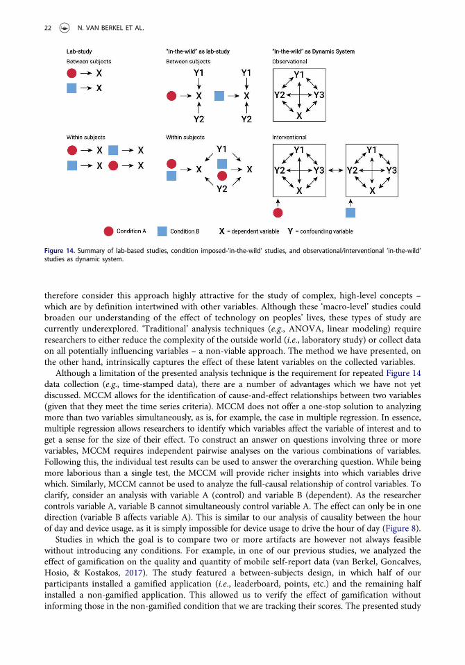
The paradigm shift of conducting research in-the-wild rather than in a laboratory has resonatedstrongly with the HCI community (Chamberlain, Crabtree, Rodden, Jones, & Rogers, 2012; Rogers,2011). In transitioning from laboratory studies to real-world observations, HCI researchers haveoften relied on the lab-based practice of introducing conditions to their study designs. We summar-ize common study configurations for lab-based and ‘in-the-wild’ studies in Figure 14. Introducingconditions ‘in-the-wild’ does however introduce an interesting incongruity: imposing artificial studyconditions upon participants as we attempt to study them in a naturalistic environment. This level of‘undisturbed’ observation is typically seen in ethnographic research but rarely in empirical work.

We believe that using the analysis method presented in this paper, researchers can achieve a betterunderstanding of their participants’ interaction with technology without the need for experimentalconditions. This approach, sometimes labeled as computational ethnography, compels us to rethinkthe design and goals of experiments in HCI. Conceptualizing the participant’s world as a dynamicsystem allows us to study this environment without introducing artificial conditions in the partici-pant’s world to determine significant effects. Our method allows us to identify relationships betweenvariables and obtain a higher-level understanding of the participant’s interaction with technology.Arguably this approach is more compelling to use when studying macro-level behaviors, such as inthe case of digital phenotyping, rather than micro-level behaviors, such as text entry usability. We


therefore consider this approach highly attractive for the study of complex, high-level concepts –which are by definition intertwined with other variables. Although these ‘macro-level’ studies couldbroaden our understanding of the effect of technology on peoples’ lives, these types of study arecurrently underexplored. ‘Traditional’ analysis techniques (e.g., ANOVA, linear modeling) requireresearchers to either reduce the complexity of the outside world (i.e., laboratory study) or collect dataon all potentially influencing variables – a non-viable approach. The method we have presented, onthe other hand, intrinsically captures the effect of these latent variables on the collected variables.

Although a limitation of the presented analysis technique is the requirement for repeated Figure 14data collection (e.g., time-stamped data), there are a number of advantages which we have not yetdiscussed. MCCM allows for the identification of cause-and-effect relationships between two variables(given that they meet the time series criteria). MCCM does not offer a one-stop solution to analyzingmore than two variables simultaneously, as is, for example, the case in multiple regression. In essence,multiple regression allows researchers to identify which variables affect the variable of interest and toget a sense for the size of their effect. To construct an answer on questions involving three or morevariables, MCCM requires independent pairwise analyses on the various combinations of variables.Following this, the individual test results can be used to answer the overarching question. While beingmore laborious than a single test, the MCCM will provide richer insights into which variables drivewhich. Similarly, MCCM cannot be used to analyze the full-causal relationship of control variables. Toclarify, consider an analysis with variable A (control) and variable B (dependent). As the researchercontrols variable A, variable B cannot simultaneously control variable A. The effect can only be in onedirection (variable B affects variable A). This is similar to our analysis of causality between the hourof day and device usage, as it is simply impossible for device usage to drive the hour of day (Figure 8).

Studies in which the goal is to compare two or more artifacts are however not always feasiblewithout introducing any conditions. For example, in one of our previous studies, we analyzed theeffect of gamification on the quality and quantity of mobile self-report data (van Berkel, Goncalves,Hosio, & Kostakos, 2017). The study featured a between-subjects design, in which half of ourparticipants installed a gamified application (i.e., leaderboard, points, etc.) and the remaining halfinstalled a non-gamified application. This allowed us to verify the effect of gamification withoutinforming those in the non-gamified condition that we are tracking their scores. The presented study

Figure 14. Summary of lab-based studies, condition imposed-‘in-the-wild’ studies, and observational/interventional ‘in-the-wild’studies as dynamic system.


design is typical in the current HCI landscape, in which two artifacts are compared by analyzingtheir respective effect on participants in-the-wild. As MCCM does not allow for a direct analysis ofvariables across conditions, one can run a separate analysis for each category and a variable ofinterest. Doing so for a binary categorical variable (in our example: gamified or non-gamified) willgenerate two separate plots, identifying the relationship of interest for each condition. Then, basedon these plots and summarized results, it is possible to compare the direction and effect of a variableof interest between two conditions. We label this approach as ‘interventional’ in Figure 14. The sameapproach can be used to analyze differences in causal relationships between other categoricalvariables (e.g., testing for differences in gender, geography, or other demographics).

Rather than analyzing categorical variables which have already been established (e.g., conditions,gender, etc.), the proposed visualization method can be used to visually identify unknown clusters inthe dataset if they exist. For example, we know from the literature that people use their mobiledevices differently, and researchers have applied clustering to identify these differences (Goncalves,Hosio, van Berkel, Ahmed, & Kostakos, 2017; Visuri et al., 2017; Zhao et al., 2016). Clusters canemerge in the analysis as a group of participants for which the relationship between variables is inthe opposite direction or off different strength. For example, while for a large majority of partici-pants in our smartwatch dataset their battery level is driven by smartwatch usage – a cluster ofparticipants emerges with an opposite relationship in which battery level drives device usage.

4.4. Weaknesses and limitations

The analysis technique presented in this paper relies on time series data. The collection of such a datasetrequires repeated measurements over a period of time. Therefore, this method of analysis is only suitablefor studies in which participants are observed and (continuously) tracked for an extended period of time.Data which is collected through one-off surveys, interviews, or otherwise missing a repetitive nature ofdata collection cannot be used in combination with CCM. The suitable granularity for time seriesanalysis is dependent both on the richness of the data and the total duration of the study. In ourevaluation of Dataset 2, in which there was a wide dissimilarity in the duration of data collection betweenparticipants, we observe many ‘discarded’ participants as the result of insufficient data (see Figures 6–8).We opted to analyze our results without filtering out these participants to highlight the robustness of themethod. Although it would not change the ultimate outcome of the direction of causality (discardedparticipants are not considered for this), future usage of this method may consider specifying theexclusion criteria of participants prior to analysis and not include these in the MCCM procedure.Through our analysis of Dataset 3, we show how this method can be applied in laboratory studies ona task-based granularity as opposed to a time-based delimiter (e.g., minutes, hours).

In addition, the technique requires adequate volumes of data for each participant. In our analyses,we use a threshold of at least 10 data points per participant, but more stringent requirements mightincrease this to 20 or even 30 to obtain adequate coverage of a dynamic systems for each individual.These may be the number of points in a time series dataset (per each variable), or can be the numberof distinct tasks that the participant was observed doing. In our experience, the datasets tend to failthe heuristics when they have fewer data, and additionally, the number of observations limits thesearch space for E (embedding dimension).

Finally, we have described how CCM can only analyze pairwise relationships, unlike multiplelinear regression where multiple variables can be considered. In the presence of multiple variables,one has to conduct multiple pairwise analyses between the outcome variable and each of thevariables of interest.

5. Conclusion

In this paper, we present the use of Multiple Convergent Cross Mapping (MCCM) for the analysis ofhuman behavior in HCI. While the basis of MCCM has been in active use in other scientific fields,


most prominently in Ecology, it has never been applied to HCI. By analyzing time-series data of twovariables, MCCM is able to detect the causality between these two variables and identify which of thetwo dominates. Whereas CCM has previously been applied to analyze single ecosystems, MCCM cansummarize and visualize a large number of ecosystems (ergo, participants), as user studies in HCItypically involve multiple participants. Our analysis shows how these results could reveal interestinginformation about a participant population and present results on two in-the-wild studies,a laboratory study, and an artificial dataset. We revisit previously carried out data analyses andfind examples where a high correlation does not result in causation. In addition, we show that ouranalysis method can reveal differences in the population (e.g., clustering behavior). Finally, wepresent various sanity checks to verify the validity of our approach.

We believe our analysis method will be useful for a variety of study designs in HCI. For laboratorystudies, we show how our technique can be useful to establish causality between two variables even in theabsence of explicit time series data by analyzing experimental data on a task-level. For in-the-wild studies,weidentify two additional changes in perspective. First, rather than imposing research conditions, and thusaffecting the in situ observation of participants, the presented analysis method allows researchers to betterunderstand the complex interaction between people and technology without inferring about the partici-pant’s low-level interaction with technology. Second, instead of utilizing a unidirectional analysis such asregression (inwhich one variable is the dependent variable), CCMallows for a bidirectional analysiswithoutthe problematic assumptions associated with Granger causality. Crucially, the presented analysis accountsfor latent variables, and therefore researchers can be selective in which variables they capture or analyze.Weargue that, similar to the relationships identified in ecological systems, the relationship between a humanand a technological artifactmay often be bidirectional rather than unidirectional. Using the presented EDMandCCM analysis methods, researchers can identify these relationships and achieve a better understandingof the interactions between humans and technology while making minimal assumptions about the formthese interactions take over time.

HCI editorial record

First received on <date>. Revisions received on <date>, <date>, and <date>. Accepted by <action-editor-name>. Finalmanuscript received on <date>. – Editor

Funding

This work is partially funded by a Samsung Global Research Outreach grant, and the ARC Discovery Project[DP190102627]; Australian Research Council [ARC Discovery Project DP190102627]; Samsung [Samsung GlobalResearch Outreach grant].

Notes on contributors

Niels van Berkel ([email protected], www.nielsvanberkel.com) is a computer scientist with an interest inubiquitous computing, social computing, and human-computer interaction; he is an Assistant Professor at AalborgUniversity.

Simon Dennis ([email protected]) is a cognitive psychologist with an interest in memory, language, andbig-data; he is a Professor at The University of Melbourne.

Michael Zyphur ([email protected]) is a statistician and industrial-organizational psychologist with aninterest in statistical modeling and probability; he is an Assistant Professor at The University of Melbourne.

Jinjing Li ([email protected], http://www.jinjingli.com/) is an economist with an interest in economic modeling,simulation, and policymaking; he is an Associate Professor at the University of Canberra.

Andrew Heathcote ([email protected]) is a cognitive psychologist with an interest in decision making,sensory processes, and psychological methodology; he is a Professor at The University of Tasmania.


Vassilis Kostakos ([email protected], https://people.eng.unimelb.edu.au/vkostakos/) is a computerscientist with an interest in with an interest in ubiquitous computing, social computing, and human-computer interac-tion; he is a Professor at The University of Melbourne.

ORCID

Niels van Berkel http://orcid.org/0000-0001-5106-7692Vassilis Kostakos http://orcid.org/0000-0003-2804-6038

References

Bennett, C. M., Miller, M. B., & Wolford, G. L. (2009). Neural correlates of interspecies perspective taking in thepost-mortem Atlantic Salmon: An argument for multiple comparisons correction. NeuroImage, 47, S39–S41.doi:10.1016/S1053-8119(09)71202-9

van Berkel, N., Goncalves, J., Hosio, S., & Kostakos, V. (2017). Gamification of mobile experience sampling improvesdata quality and quantity. Proceedings of the ACM on Interactive, Mobile, Wearable and Ubiquitous Technologies, 1(3), 1–21. doi:10.1145/3130972

van Berkel, N., Goncalves, J., Lovén, L., Ferreira, D., Hosio, S., & Kostakos, V. (2018). Effect of experience samplingschedules on response rate and recall accuracy of objective self-reports. International Journal of Human-computerStudies, 125, 118–128. doi:10.1016/j.ijhcs.2018.12.002

Cairns, P. (2019). Doing better statistics in human-computer interaction. Cambridge, UK: Cambridge University Press.doi:10.1017/9781108685139

Carpenter, S. R., & Brock, W. A. (2006). Rising variance: A leading indicator of ecological transition. Ecology Letters, 9(3), 311–318. doi:10.1111/j.1461-0248.2005.00877.x

Carroll, J. M. (2000). Making use: scenario-based design of human-computer interactions. Cambridge, United States:MIT press.

Chamberlain, A., Crabtree, A., Rodden, T., Jones, M., & Rogers, Y. 2012. Research in the wild: Understanding ‘In thewild’ approaches to design and development. In Proceedings of the Designing Interactive Systems Conference (DIS),Newcastle Upon Tyne, United Kingdom, ACM, 795–796. DOI: 10.1145/2317956.2318078

Chang, C.-W., Ushio, M., & Hsieh, C.-H. (2017). Empirical dynamic modeling for beginners. Ecological Research, 32(6), 785–796. doi:10.1007/s11284-017-1469-9

Charmaz, K. (2006). Constructing grounded theory: a practical guide through qualitative analysis. California, UnitedStates: SAGE Publications.

Clark, A. T., Ye, H., Isbell, F., Deyle, E. R., Cowles, J., Tilman, G. D., & Sugihara, G. (2015). Spatial convergent crossmapping to detect causal relationships from short time series. Ecology, 96(5), 1174–1181. doi:10.1890/14-1479.1

Clayton, R. B., Leshner, G., & Almond, A. (2015). The extended iSelf: The impact of iPhone separation on cognition,emotion, and physiology. Journal of Computer-Mediated Communication, 20(2), 119–135. doi:10.1111/jcc4.12109

Corbin, J., & Strauss, A. (2008). Basics of qualitative research (3rd ed.): techniques and procedures for developinggrounded theory. Thousand Oaks, California: SAGE Publications. doi:10.4135/9781452230153

Cramer, A. O. J., van Borkulo, C. D., Giltay, E. J., van der Maas, H. L. J., Kendler, K. S., Scheffer, M., & Borsboom, D.(2016). Major depression as a complex dynamic system. PloS One, 11(12), e0167490. doi:10.1371/journal.pone.0167490

DeAngelis, D. L., & Yurek, S. (2015). Equation-free modeling unravels the behavior of complex ecological systems.Proceedings of the National Academy of Sciences, 112(13), 3856–3857. doi:10.1073/pnas.1503154112

Deyle, E. R., May, R. M., Munch, S. B., & Sugihara, G. (2016). Tracking and forecasting ecosystem interactions in realtime. Proceedings of the Royal Society B: Biological Sciences, 283(1822), 20152258. doi:10.1098/rspb.2015.2258

Dix, A., Finlay, J. E., Abowd, G. D., & Beale, R. (2003). Human-computer interaction (3rd ed. Harlow, UK: PearsonEducation Limited.

Dörnyei, Z., Henry, A., & MacIntyre, P. D. (2014). Motivational dynamics in language learning. UK:MultilingualMatters. Bristol.

Ferreira, D., Dey, A. K., & Kostakos, V. 2011. Understanding human-smartphone concerns: A study of battery life. InInternational Conference on Pervasive Computing, 19–33. San Francisco, California. doi:10.1007/978-3-642-21726-5_2

Galea, S., Riddle, M., & Kaplan, G. A. (2010). Causal thinking and complex system approaches in epidemiology.International Journal of Epidemiology, 39, 97–106. doi:10.1093/ije/dyp296

Gaver, W. W. 1991. Technology affordances. In Proceedings of the SIGCHI Conference on Human Factors inComputing Systems, New Orleans, Louisiana, USA, ACM, 79–84. DOI: 10.1145/108844.108856

Gibson, J. J. (1979). The ecological approach to visual perception. New York, NY: Psychology Press.


https://doi.org/10.1016/S1053-8119(09)71202-9

https://doi.org/10.1145/3130972

https://doi.org/10.1016/j.ijhcs.2018.12.002

https://doi.org/10.1017/9781108685139

https://doi.org/10.1111/j.1461-0248.2005.00877.x

https://doi.org/10.1145/2317956.2318078

https://doi.org/10.1007/s11284-017-1469-9

https://doi.org/10.1890/14-1479.1

https://doi.org/10.1111/jcc4.12109

https://doi.org/10.4135/9781452230153

https://doi.org/10.1371/journal.pone.0167490

https://doi.org/10.1371/journal.pone.0167490

https://doi.org/10.1073/pnas.1503154112

https://doi.org/10.1098/rspb.2015.2258

https://doi.org/10.1007/978-3-642-21726-5_2

https://doi.org/10.1007/978-3-642-21726-5_2

https://doi.org/10.1093/ije/dyp296

https://doi.org/10.1145/108844.108856

Goncalves, J., Hosio, S., van Berkel, N., Ahmed, F., & Kostakos, V. (2017). CrowdPickUp: Crowdsourcing task pickupin the wild. Proceedings of the ACM on Interactive, Mobile, Wearable and Ubiquitous Technologies, 1(3), 51:51–51:22. doi:10.1145/3130916

Granger, C. W. J. (1969). Investigating causal relations by econometric models and cross-spectral methods.Econometrica, 37(3), 424–438. doi:10.2307/1912791

Hosio, S., Ferreira, D., Goncalves, J., van Berkel, N., Luo, C., & Ahmed, M., … Kostakos, V. 2016. Monetaryassessment of battery life on smartphones. In Proceedings of the ACM Conference on Human Factors inComputing Systems, 1869–1880. San Jose, USA, doi:10.1145/2858036.2858285

Korb, K. B., & Nicholson, A. E. (2008). The causal interpretation of bayesian networks. In D. E. Holmes & L. C. Jain(Eds.), Innovations in bayesian networks: Theory and applications (pp. 83–116). Berlin, Heidelberg: Springer BerlinHeidelberg.

Larsen-Freeman, D. (2015). Ten ‘lessons’ from complex dynamic systems theory: what is on offer. In Z. Dörnyei, D. P.MacIntyre, & H. Alastair (Eds (Eds), Motivational dynamics in language learning (pp. pp. 11–19). Bristol, UK:Multilingual Matters.

Lazar, J., Feng, J. H., & Hochheiser, H. (2017). Research methods in human-computer interaction. In Research methodsin human-computer interaction (pp. 25–44). Wiley Publishing.

Lu, B., Zanutto, E., Hornik, R., & Rosenbaum, P. R. (2001). Matching with doses in an observational study of a mediacampaign against drug abuse. Journal of the American Statistical Association, 96(456), 1245–1253. doi:10.1198/016214501753381896

Mauboussin, M. J. (2002). Revisiting market efficiency: The stock market as a complex adaptive system. Journal ofApplied Corporate Finance, 14(4), 47–55. doi:10.1111/j.1745-6622.2002.tb00448.x

Mehrotra, A., Pejovic, V., Vermeulen, J., Hendley, R., & Musolesi, M. 2016. My phone and me: Understanding people’sreceptivity to mobile notifications. In Proceedings of the ACM Conference on Human Factors in Computing Systems,Santa Clara, California, USA, ACM, 1021–1032. DOI: 10.1145/2858036.2858566

Mehrotra, A., Tsapeli, F., Hendley, R., & Musolesi, M. (2017). MyTraces: Investigating correlation and causationbetween users’ emotional states and mobile phone interaction. Proceedings of the ACM on Interactive, Mobile,Wearable and Ubiquitous Technologies (IMWUT), 1(3), 83: 81–83:21. doi:10.1145/3130948

Mønster, D., Fusaroli, R., Tylén, K., Roepstorff, A., & Sherson, J. F. 2016. Inferring causality from noisy time seriesdata - A test of convergent cross-mapping. In Proceedings of the 1st International Conference on ComplexInformation Systems (COMPLEXIS), 48–56. Rome, Italy.

Norman, D. A. (1986). Cognitive Engineering. In D. A. Norman & S. W. Draper (Eds.), User centered system design:New perspectives on human-computer interaction (pp. 31–61). Hillsdale, NJ: Lawrence Erlbaum Associates.

Norman, D. A. (2002). The design of everyday things. New York, NY: Basic Books.Pearl, J. (2009). Causality: models, reasoning and inference. Cambridge, United Kingdom: Cambridge University Press.

doi:10.1017/CBO9780511803161Popkin, G., 2015. A twisted path to equation-free prediction. Retrieved from https://www.quantamagazine.org/chaos-

theory-in-ecology-predicts-future-populations–20151013/Rogers, Y. (2011). Interaction design gone wild: Striving for wild theory. Interactions, 18(4), 58–62. doi:10.1145/

1978822.1978834Sarsenbayeva, Z., van Berkel, N., Visuri, A., Rissanen, S., Rintamaki, H., Kostakos, V., & Goncalves, J. (2017). Sensing

cold-induced situational impairments in mobile interaction using battery temperature. Proceedings of the ACM onInteractive, Mobile, Wearable and Ubiquitous Technologies (IMWUT), 1(3), 98: 91–98:99. doi:10.1145/3130963

Small, M., & Tse, C. K. (2003). Detecting determinism in time series: The method of surrogate data. IEEE Transactionson Circuits and Systems I: Fundamental Theory and Applications, 50(5), 663–672. doi:10.1109/TCSI.2003.811020

Stothart, C., Mitchum, A., & Yehnert, C. (2015). The attentional cost of receiving a cell phone notification. Journal ofExperimental Psychology: Human Perception and Performance, 41(4), 893–897. doi:10.1037/xhp0000100

Sugihara, G. (1994). Nonlinear forecasting for the classification of natural time series. Philosophical Transactions of theRoyal Society of London. Series A: Physical and Engineering Sciences, 348(1688), 477–495. doi:10.1098/rsta.1994.0106

Sugihara, G., May, R., Ye, H., Hsieh, C.-H., Deyle, E., Fogarty, M., & Munch, S. (2012). Detecting causality in complexecosystems. Science, 338(6106), 496–500. doi:10.1126/science.1227079

Takens F. (1981) Detecting strange attractors in turbulence. In: Rand D., Young LS. (eds) Dynamical Systems andTurbulence, Warwick 1980. Lecture Notes in Mathematics, vol 898. Springer, Berlin, Heidelberg.

Tsapeli, F., & Musolesi, M. (2015). Investigating causality in human behavior from smartphone sensor data: Aquasi-experimental approach. EPJ Data Science, 4(24), 1–15. doi:10.1140/epjds/s13688-015-0061-1

Tsapeli, F., Musolesi, M., & Tino, P. (2017). Model-free causality detection: An application to social media andfinancial data. Physica A: Statistical Mechanics and Its Applications, 483, 139–155. doi:10.1016/j.physa.2017.04.101

Tsonis, A. A., Deyle, E. R., Ye, H., & Sugihara, G. (2018). Convergent cross mapping: theory and an example. In A. A.Tsonis (Ed (Ed), Advances in nonlinear geosciences (pp. pp. 587–600). Cham, Switzerland: Springer InternationalPublishing. doi:10.1007/978-3-319-58895-7


https://doi.org/10.1145/3130916

https://doi.org/10.2307/1912791

https://doi.org/10.1145/2858036.2858285

https://doi.org/10.1198/016214501753381896

https://doi.org/10.1198/016214501753381896

https://doi.org/10.1111/j.1745-6622.2002.tb00448.x

https://doi.org/10.1145/2858036.2858566

https://doi.org/10.1145/3130948

https://doi.org/10.1017/CBO9780511803161

https://www.quantamagazine.org/chaos-theory-in-ecology-predicts-future-population

https://www.quantamagazine.org/chaos-theory-in-ecology-predicts-future-population

https://doi.org/10.1145/1978822.1978834

https://doi.org/10.1145/1978822.1978834

https://doi.org/10.1145/3130963

https://doi.org/10.1109/TCSI.2003.811020

https://doi.org/10.1037/xhp0000100

https://doi.org/10.1098/rsta.1994.0106

https://doi.org/10.1126/science.1227079

https://doi.org/10.1140/epjds/s13688-015-0061-1

https://doi.org/10.1016/j.physa.2017.04.101

https://doi.org/10.1007/978-3-319-58895-7

Visuri, A., Sarsenbayeva, Z., van Berkel, N., Goncalves, J., Rawassizadeh, R., Kostakos, V., & Ferreira, D. 2017.Quantifying sources and types of smartwatch usage sessions. In Proceedings of the SIGCHI Conference onHuman Factors in Computing Systems (CHI), 3569–3581. Colorado, United States doi:10.1145/3025453.3025817

Visuri, A., van Berkel, N., Goncalves, J., Luo, C., Ferreira, D., & Kostakos, V. 2017. Predicting interruptibility formanual data collection: A cluster-based user model. In Proceedings of the ACM Conference on Human-ComputerInteraction with Mobile Devices and Services, ACM, Article 12. Vienna, Austria doi:10.1145/3098279.3098532

Wobbrock, J. O., & Kientz, J. A. (2016). Research contributions in human-computer interaction. Interactions, 23(3),38–44. doi:10.1145/2907069

Ye, H., Beamish, R. J., Glaser, S. M., Grant, S. C. H., Hsieh, C.-H., Richards, L. J., … Sugihara, G. (2015). Equation-freemechanistic ecosystem forecasting using empirical dynamic modeling. Proceedings of the National Academy ofSciences, 112(13), 1569–1576. doi:10.1073/pnas.1417063112

Ye, H., Clark, A., Deyle, E., Munch, S., Keyes, O., & Cai, J., … Sugihara, G., 2019. rEDM: Applications of empiricaldynamic modeling from time series. Retrieved from https://CRAN.R-project.org/package=rEDM

Zhao, S., Ramos, J., Tao, J., Jiang, Z., Li, S., & Wu, Z., … Dey, A. K. 2016. Discovering different kinds of smartphoneusers through their application usage behaviors. In Proceedings of the ACM International Joint Conference onPervasive and Ubiquitous Computing (UbiComp), ACM, 498–509. Heidelberg, Germany doi:10.1145/2971648.2971696


https://doi.org/10.1145/3025453.3025817

https://doi.org/10.1145/3098279.3098532

https://doi.org/10.1145/2907069

https://doi.org/10.1073/pnas.1417063112

https://doi.org/10.1145/2971648.2971696

https://doi.org/10.1145/2971648.2971696

Date post:	03-Apr-2022
Category:	Documents
Upload:	others
View:	6 times
Download:	0 times

Modeling interaction as a complex system

Documents