2021, VOL. 5, NO: 3, 244-253

244

e-ISSN: 2587-0963 www.ijastech.org

Modelling and Simulation of Detailed Vehicle Dynamics for

the Development of Innovative Powertrains

Shantanu Pardhi1*, Ajinkya Deshmukh1 and Hugo Ajrouche1

0000-0002-6325-2796, 0000-0002-0401-9521, 0000-0001-9414-0247 1 Altran Prototypes Automobiles, Hybrid Innovative Powertrain, Research & Innovation Department, ALTRAN part of Capgemini-France. 2 Rue Paul Dautier, 78140 Vélizy-Villacoublay, France

1. Introduction

With an ever-increasing application of new and innovative con-

cepts in the powertrain domain for fulfilling the needs of fuel effi-

ciency, reduced pollution, road safety, performance and drivability,

the automotive industry is relying more and more on mathematical

simulations for faster, cost-effective, and easier adaptations [1]. A

rudimentary representation of vehicle dynamics has been found to

be effective in the early project phase for low level powertrain sim-

ulation activities such as new concept application, assessing the

working range and understanding initial control requirements un-

der normal driving. Once this is achieved, a need for higher preci-

sion arises for not only further minimizing energy losses or finding

reasons for emission peaks, but also for analysing the impact of

this concept integration on other important vehicle characteristics

such as road safety, drivability and performance, which are more

pronounced under extreme driving conditions [2].

To simulate the detailed longitudinal vehicle dynamics, research

has been done on various modelling methodologies for taking into

account the effect of transient behaviour of different components

on the complete powertrain. Majdoub et al. (2011) have shown

control-oriented vehicle dynamics state-space representation with

Kiencke’s tyre slip model for speed regulation using a nonlinear

controller [3]. Real time tyre friction and slip estimation technique

and its integration for varying ABS control to achieve higher brak-

ing performance is given by Singh et al. (2015) [4]. The effect of

steady state and transient vehicle dynamics modelling on quarter

wheel model is discussed by Jansen et al. (2010) which could be

used for robust ABS simulation and development [5]. Shakouri et

al. (2010) have presented a vehicle dynamics modelling method

with normal load transfer using balance of moments around wheel

contact points [6]. James et al. (2020) have compared the results of

physical and data driven models with real tests and have shown

Research Article

https://doi.org/10.30939/ijastech..931066

Received 01.05.2021

Revised 00.00.2020 Accepted 27.00.2020

* Corresponding author

Shantanu Pardhi

shantanu.pardhi@vub.be

Altran Prototypes Automobiles, Hybrid

Innovative Powertrain, Research & Inno-

vation Department, ALTRAN part of

Capgemini-France. 2 Rue Paul Dautier,

78140 Vélizy-Villacoublay, France

Tel: +33605706711

Pardhi et al. / International Journal of Automotive Science and Technology 5 (3): 244-253, 2021

245

better outcome with the later for specific use cases [7].

The vehicle dynamics modelling technique proposed in this

work fulfils simulation needs for the advanced stages of a project

while still maintaining a simple and understandable level of mod-

elling complexity. The main originality of this work includes the

integration of suitable modelling methods from the literature along

with an uncommon trivial suspension representation using the bal-

ance of various force moments and vehicle motion around its cen-

tre of gravity (CoG). The precise simulation of dynamic effects and

losses in wheels and other vehicle components make this method

highly effective for the authors’ ongoing transient analysis and de-

velopment activities such as improving regenerative braking under

heavy deceleration or optimizing P4 hybrid powertrain road charg-

ing modes in dynamic driving. Its application can be extended to

even early controls architecture development and calibration for

braking, traction modules, and electronic safety measures along

with their validation before implementation on a real system [5].

Its scope can also cover testing of existing Electronic Control Unit

strategies and functions using Model In the Loop (MIL) and Soft-

ware In the Loop applications (SIL) [1].

This article is divided into several sections. Section 2 explains

the selected approach with zero-dimensional modelling of the front

and rear wheel dynamics including the effect of tyre slip, transmis-

sible force and rotational inertia, front – rear normal load transfer

modelling using a trivial suspension depiction and a robust repre-

sentation of different tractive resistances. Section 3, shows a sim-

plified way of representing electronic vehicle safety and drivability

systems for taking into account their effect on the vehicle dynam-

ics while avoiding their high level of functional complexity. Sec-

tion 4 presents the results of the use case vehicle simulation under

normal and drastic driving conditions and finally the conclusion

and some future perspectives are provided in section 5.

2. Modelling methodology

A modular and generic modelling approach has been used to

make sure that the proposed methodology is able to simulate the

working of various possible means of upcoming propulsion tech-

nologies such as electric, thermal, hybrid or even fuel cell for ve-

hicle applications ranging from small scooters to heavy-duty

trucks. This also facilitates easy integration of any vehicle archi-

tecture such as front, rear or all-wheel drive and to study the be-

haviour and dynamics of individual components and their impact

on the functioning of the complete powertrain. For longitudinal ve-

hicle dynamics, a dynamic forward type modelling approach based

on analytical representations has been selected. It undertakes a

fixed discrete-time steps simulation, instead of linear data-driven

correlations running at continuous time, to fulfil the objectives of

modularity, generic representation and ease of sizing while main-

taining a close comparison with real-world applications [7].

The platform consists of a vehicle block for calculating the ef-

fects of tractive resistances on vehicle speed. It consists of two sep-

arate wheel blocks representing lumped front and rear wheels in-

cluding the effect of slips and rotational inertias (two-wheel ap-

proach) and a vertical load transfer model for finding instantaneous

normal load distribution on the front and rear during vehicle mo-

tion (fig. 1). An in-house driver block has also been integrated to

obtain accelerator and brake pedal commands depending on the

difference between the actual vehicle speed and the desired speed.

Since the model is forward and dynamic in nature, the driver com-

mands could also be given by real human intervention through

Driver In the Loop (DIL) approach. Using these commands, the

powertrain and brake blocks develop tractive and braking torque

respectively. Two identical brake models are used to separately

represent braking of front and rear wheels. The powertrain for this

case is considered as an ideal torque source that can instantane-

ously give any desired torque request within its functional limits,

with the idea of being able to replace it with a detailed model of an

actual prime mover. Torque from the powertrain and brakes are

transmitted to front and rear wheels according to the chosen vehi-

cle architecture and depending on their dynamics transferred to the

road as tractive/braking force creating a reaction on the vehicle and

affecting its speed. The instantaneous vehicle speed, which de-

pends on the wheel dynamics, then becomes angular wheel speed

and is connected back to the powertrain and brakes. Thus, the

model works in an action (torque) – reaction (speed) manner and

can be used to precisely represent actual vehicle behaviour.

Fig. 1. Longitudinal vehicle dynamics model architecture

2.1 Wheel model

The wheel model calculates the amount of tractive force that the

tyres transmit to the road for the vehicle to attain the desired speed

and also the actual angular wheel speeds which are different from

Pardhi et al. / International Journal of Automotive Science and Technology 5 (3): 244-253, 2021

246

the vehicle speed on account of wheel slip. Under standard operat-

ing conditions (road properties) tyres have been found to follow a

certain relation between the amount of force transferred to the road

𝐹𝑥 and their slip 𝑘. The amount of force transmitted also tends to

be directly proportional to the normal vertical load on the wheel

𝐹𝑧 and the tyre friction coefficient 𝜇 (Eq. 1).

𝐹𝑥 = 𝐹𝑧 𝜇 (1)

𝐹𝑧 = 𝑚𝑣 𝑔 (2)

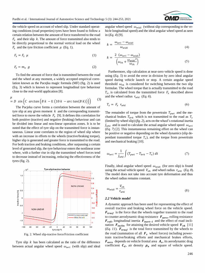
To find the amount of force that is transmitted between the road

and the wheel at any moment, a widely accepted empirical corre-

lation known as the Pacejka magic formula (MF) (fig. 2) is used

(Eq. 3) which is known to represent longitudinal tyre behaviour

close to the real-world application [8].

𝜇= 𝐷 𝑠𝑖𝑛 (C 𝑎𝑟𝑐𝑡𝑎𝑛 (𝐵 𝑘 − E (10 𝑘 − 𝑎𝑟𝑐 𝑡𝑎𝑛 (𝐵 𝑘))))

(3)

The Pacjeka curve forms a correlation between the amount of

tyre slip at any given moment 𝑘 and the corresponding transmit-

ted force to move the vehicle 𝐹𝑥 [9]. It defines this correlation for

both positive (tractive) and negative (braking) behaviour and can

be divided into linear and non-linear operation zones. It is to be

noted that the effect of tyre slip on the transmitted force is instan-

taneous. Linear zone correlates to the region of wheel slip where

with an increase in efforts to the wheels (tractive/braking torque),

higher slip is generated and greater force is transmitted to the road.

For both traction and braking conditions, after surpassing a certain

level of generated slip, the tyre behaviour enters the nonlinear zone

where, with a further rise in slip the transmitted wheel forces tend

to decrease instead of increasing, reducing the effectiveness of the

tyres (fig. 2).

Fig. 2. Wheel slip-tractive force/Friction coefficient

Tyre slip 𝑘 has been calculated as the ratio of the difference

between actual angular wheel speed 𝜔𝑤𝑟𝑙 (with slip) and ideal

angular wheel speed 𝜔𝑤𝑖𝑑𝑙 (without slip corresponding to the ve-

hicle longitudinal speed) and the ideal angular wheel speed as seen

in (Eq. 4) [9].

𝑘 = 𝜔𝑤𝑟𝑙 − 𝜔𝑤𝑖𝑑𝑙

𝜔𝑤𝑖𝑑𝑙

𝑘 = 2 (𝜔𝑤𝑟𝑙 − 𝜔𝑤𝑖𝑑𝑙)

(𝜔𝑡ℎ +𝜔𝑤𝑖𝑑𝑙

2

𝜔𝑡ℎ)

Furthermore, slip calculation at near-zero vehicle speed is done

using (Eq. 5) to avoid the error in division by zero ideal angular

speed during vehicle launch or stop. A certain angular speed

threshold 𝜔𝑡ℎ is considered for switching between the two slip

formulae. The wheel torque that is actually transmitted to the road

𝑇𝑥 , is calculated from the transmitted force 𝐹𝑥 described above

and the wheel radius 𝑟𝑤ℎ𝑙 (Eq. 6).

𝑇𝑥 = 𝐹𝑥 𝑟𝑤ℎ𝑙

The remainder of torque from the powertrain 𝑇𝑝𝑤𝑡 and the me-

chanical brakes 𝑇𝑏𝑟𝑘 which is not transmitted to the road as 𝑇𝑥

(limited by wheel slip) (fig. 2), acts on the wheel’s rotational inertia

𝐽𝑤ℎ𝑙 and is used to calculate the actual angular wheel speed 𝜔𝑤𝑟𝑙

(Eq. 7) [2]. This instantaneous remaining effort on the wheel can

be positive or negative depending on the wheel dynamics (slip de-

pendant transmitted torque 𝑇𝑥), and the torque from powertrain

and mechanical braking [10].

𝜔𝑤𝑟𝑙 =1

𝐽𝑤ℎ𝑙

∫(𝑇𝑝𝑤𝑡 − 𝑇𝑏𝑟𝑘 − 𝑇𝑥) 𝑑𝑡

Finally, ideal angular wheel speed 𝜔𝑤𝑖𝑑𝑙 (for zero slip) is found

using the actual vehicle speed 𝑉𝑣ℎ and wheel radius 𝑟𝑤ℎ𝑙 (Eq. 8).

The model does not take into account tyre deformation and thus

the wheel radius remains constant.

𝜔𝑤𝑖𝑑𝑙 =𝑉𝑣ℎ

𝑟𝑤ℎ𝑙

2.2 Vehicle model

A dynamic approach has been used for representing the effect of

overall tractive and braking wheel force on the vehicle speed.

𝑭𝒕𝒓𝒏𝒔𝒇 is the force that the wheels together transmit to the road

to counter aerodynamic drag resistance 𝑭𝒂𝒆𝒓𝒐, rolling resistance

𝑭𝒓𝒐𝒍𝒍, longitudinal inertia 𝑭𝒊𝒏𝒆𝒓𝒕−𝒍 and the effect of road incli-

nation 𝑭𝒊𝒏𝒄𝒍𝒊𝒏 for attaining the desired vehicle speed 𝑽𝒗𝒉 [11]

(Eq. 11). 𝑭𝒕𝒓𝒏𝒔𝒇 is the total force transmitted by the wheels to

the road (summation of all 𝑭𝒙 wheel forces) including power-

train tractive/braking efforts and mechanical brakes efforts,

𝑭𝒂𝒆𝒓𝒐 depends on vehicle frontal area 𝑨𝒗, its aerodynamic drag

coefficient 𝑪𝒅 , air density 𝝆𝒂 and square of vehicle speed.

Pardhi et al. / International Journal of Automotive Science and Technology 5 (3): 244-253, 2021

247

𝑭𝒓𝒐𝒍𝒍 depends on vehicle mass 𝒎𝒗 and rolling resistance coef-

ficient of the tyres 𝑪𝒓𝒓. 𝑭𝒊𝒏𝒆𝒓𝒕−𝒍 depends on longitudinal ac-

celeration 𝒂𝒙 and vehicle mass, while 𝑭𝒊𝒏𝒄𝒍𝒊𝒏 is affected by

vehicle mass and road inclination 𝜽.

𝐹𝑡𝑟𝑛𝑠𝑓 = 𝐹𝑥𝑓 + 𝐹𝑥𝑟

𝐹𝑖𝑛𝑒𝑟𝑡−𝑙 = 𝐹𝑡𝑟𝑛𝑠𝑓 − 𝐹𝑎𝑒𝑟𝑜 + 𝐹𝑟𝑜𝑙𝑙 + 𝐹𝑖𝑛𝑐𝑙𝑖𝑛

𝑑𝑉𝑣

𝑑𝑡

=𝐹𝑡𝑟𝑛𝑠𝑓 −

12

𝜌𝑎 𝐴𝑣 𝐶𝑑 𝑉𝑣2 + 𝐶𝑟𝑟 𝑚𝑣 𝑔 𝑐𝑜𝑠𝜃 + 𝑚𝑣 𝑔 𝑠𝑖𝑛𝜃

𝑚𝑣

2.3 Load transfer model

The normal load transfer between the front and rear wheels has

been considered using a quasi-steady state approach with respect

to the pitch 𝒑𝒚 and heave 𝒛 movement of the vehicle body.

Depending on the actual vehicle speed, acceleration and the

overall applied tractive force, the model calculates the instanta-

neous vertical load on the front and rear end of the vehicle [12].

When the vehicle is stationary only the effect of position of cen-

tre of gravity (CoG) 𝒍𝒇, 𝒍𝒓, 𝒉 and road inclination 𝜽 affect the

weight distribution between front 𝑭𝒛𝒇𝟎 and rear wheels 𝑭𝒛𝒓𝟎

(Eq. 12, Eq. 13).

𝐹𝑧𝑓0 =𝑚𝑣 𝑔 (𝑙𝑟 cos(𝜃) + ℎ sin (𝜃))

𝑙𝑓 + 𝑙𝑟

𝐹𝑧𝑟0 =𝑚𝑣 𝑔 (𝑙𝑓 𝑐𝑜𝑠(𝜃) − ℎ 𝑠𝑖𝑛 (𝜃))

𝑙𝑓 + 𝑙𝑟

As the vehicle moves, the deformation of front 𝑧𝑓 and rear 𝑧𝑟

suspension creates reaction forces, which vary the load transfer on

the front 𝐹𝑧𝑓 and rear 𝐹𝑧𝑟 axles (wheels) (Eq. 14, Eq. 15). The

𝑧𝑟𝑓 and 𝑧𝑟𝑟 are suspension deformations due to vertical wheel

movement on accounts of road unevenness.

𝐹𝑧𝑓 = 𝐹𝑧𝑓0 + 𝑐𝑓(𝑧𝑟𝑓 − 𝑧𝑓)

𝐹𝑧𝑟 = 𝐹𝑧𝑟0 + 𝑐𝑟(𝑧𝑟𝑟 − 𝑧𝑟)

Pitch 𝑧 and heave 𝑝𝑦 movements are used to calculate the re-

spective suspension deformations (springs + tyres + links) for the

front 𝑧𝑓 and rear 𝑧𝑟 part of the suspension depending on the

horizontal distance of the suspensions (wheel contacts) from the

CoG (𝑙𝑓 and 𝑙𝑟) using a representation of trivial suspension (Eq.

16, Eq. 17) (fig. 3).

𝑧𝑓 = 𝑧 − 𝑙𝑓 𝑝𝑦

𝑧𝑟 = 𝑧 + 𝑙𝑟 𝑝𝑦

These pitch and heave movements are affected by the amount of

overall tractive and braking force by the wheels 𝐹𝑡𝑟𝑛𝑠𝑓, aerody-

namics drag resistance 𝐹𝑎𝑒𝑟𝑜 , height of the aerodynamic centre

ℎ𝑎, the horizontal 𝑙𝑓 , 𝑙𝑟 and vertical position of the CoG ℎ, and

the overall stiffness of the front 𝑐𝑓 and rear 𝑐𝑟 suspension

(springs + links + tyres) (Eq. 18, Eq. 19). Horizontal and vertical

balance of all forces and moments around the CoG is taken into

account to calculate vehicle pitch and heave displacements.

𝑧 = −(𝑐𝑓 𝑙𝑓 − 𝑐𝑟 𝑙𝑟)

𝑐𝑓 𝑐𝑟(𝑙𝑓 + 𝑙𝑟)2 (𝐹𝑡𝑟𝑛𝑠𝑓 ℎ + 𝐹𝑎𝑒𝑟𝑜(ℎ𝑎 − ℎ))

𝑝𝑦 = −(𝑐𝑓 + 𝑐𝑟)

𝑐𝑓 𝑐𝑟(𝑙𝑓 + 𝑙𝑟)2 (𝐹𝑡𝑟𝑛𝑠𝑓 ℎ + 𝐹𝑎𝑒𝑟𝑜(ℎ𝑎 − ℎ))

This instantaneous load on front 𝐹𝑧𝑓 and rear 𝐹𝑧𝑟 is utilised in

the respective wheel models to precisely consider its effect on the

available tyre grip for front and rear wheels and the amount of

force that they transmit 𝐹𝑥𝑓 and 𝐹𝑥𝑟 (Eq. 1) without entering the

nonlinear slipping zone (fig. 2). This approach is quasi-static

(speed of vertical vehicle movement is considered constant except

in the longitudinal direction) and thus cannot consider the damping

dynamics coming from suspension dampers, tyres, bushings, and

linkages. It does not take into account the separate effect of torque

given to the wheels by the brakes (unsprung) and powertrain ele-

ments (sprung), or the effect of separate transmitted forces from

the front and rear wheels on the suspension.

3 Control

Since the core focus of this work has been on modelling and rep-

resentation of longitudinal vehicle dynamics close to real condi-

tions, simple ways for representing the actual safety control sys-

tems for maintaining regulated vehicle functioning under normal

as well as intense driving are considered. The control depictions

have been made to just closely study their resulting behaviour on

vehicle dynamics and not their actual functioning.

3.1 Brake bias

It is evident from the case vehicle’s centre of gravity CoG posi-

tion (Sonata 2011) (Table 1) that even when the vehicle is sta-

tionary, the weight distribution is not equally shared between the

front and rear wheels.

Pardhi et al. / International Journal of Automotive Science and Technology 5 (3): 244-253, 2021

248

Table 1. Vehicle parameters

Vehicle name Hyundai Sonata 2011

Vehicle mass with driver [kg]

(𝑚𝑣) [21] 1542.4

Vehicle aero drag coefficient (𝐶𝑑) 0.28

Vehicle frontal area [m2] (𝐴𝑣) 2.13677

Aerodynamic centre height [m] (ℎ𝑎) 0.543814

Tyre data (front – rear size) 205/65/16 - 205/65/16

Wheel rotational inertia [kgm2] (𝐽𝑤ℎ𝑙) 1.06

Wheel radius [m] (𝑟𝑤ℎ𝑙) 0.3365/0.3365

Rolling resistance (𝐶𝑟𝑟) 0.012

MF tyre formula tuning parameters [6]

B / C / D / E 10 / 1 / 1.9 / 0.9

Centre of gravity COG position [m]

(front 𝑙𝑓/rear 𝑙𝑟/height ℎ) [21] 1.106678 / 1.6889 / 0.543814

Wheel base [m]

(𝑙𝑓+ 𝑙𝑟) [21] 2.79654

Static weight distribution [21] 60.4:39.6

Front/rear suspension spring rate

[N/m]

(𝑐𝑓/ 𝑐𝑟) (Assumed)

50000 / 50000

Maximum overall braking torque [Nm]

(Assumed) 6200

Fig. 3. Trivial suspension load transfer model

While decelerating, with the wheels stopping the vehicle and the

placement of CoG pushing it forward, the vehicle tends to be

thrown ahead and there is load transfer from the rear to the front

suspension. This creates an even larger gap between the vertical

load on the front and rear wheels and thus their ability to trans-

mit force to the road (Eq. 5). To achieve the highest possible

braking performance and road safety, this effect is taken into ac-

count and the amount of braking efforts distributed between the

front and rear are altered accordingly. Brake bias is the propor-

tion of braking efforts distributed between front and rear brakes

to achieve the desired braking performance while maintaining

vehicle stability [12]. In the case of a passenger vehicle, it is

preferred that under heavy braking if the wheels are not able to

maintain grip, it should be the front wheels that stop rotating

(lockup) instead of or before the rear wheels for avoiding lateral

instability and assuring occupant safety. For this application, a

first calibration of brake bias has been achieved for making sure

that in case of the reduced road - tyre friction (80%) for no mat-

ter how hard the brake pedal is applied, the above safety condi-

tion is met. Due to the lack of data, the operating range of the

overall braking system (braking torque) was defined so that in

case of heavy braking under normal running conditions (100%

road friction), the wheel lockup limits should arise at around

80 % of brake pedal input [12].

3.2 Electronic brake force distribution

Electronic Brake force Distribution (EBD) system or P-valve

control the instantaneous brake force distribution between front

and rear brake sets by decreasing braking efforts to the rear on

increasing deceleration to avoid rear wheel lockup due to normal

load transfer. Maintaining a less drastic brake bias under normal

driving conditions helps to obtain smoother drivability and ex-

tends the life of components such as tyres and brakes. Whereas,

an extreme brake distribution is useful in maintaining vehicle

grip, stability and safety under heavy braking by avoiding rear

lockup.

Fig. 4. Varying brake bias to avoid rear wheel lock up

(simple feed forward EBD)

The EBD depiction for this case was a simple feedforward system

which is directly based on the brake pedal input with the intention

of resembling real vehicle behaviour while avoiding control sys-

tem complexity. A first-level calibration for varying brake distri-

bution was made by testing braking performance under reduced

(80%) and normal (100%) road friction for varying brake pedal

inputs to make sure that in case of a lockup the front wheels always

lock instead of or before the rear wheels (fig. 4)

Pardhi et al. / International Journal of Automotive Science and Technology 5 (3): 244-253, 2021

249

.

Fig. 5: Longitudinal/Vertical dynamics WLTC (1020s-1460s)

3.3 Anti-lock braking system

In emergency braking or during aggressive deceleration, if a

high level of braking torque is applied to the wheels, they may

enter the nonlinear zone of functioning after surpassing a certain

level of elevated negative slip. With further increase in the wheel

slip, the transmissible force to the road will start decreasing and

there will be an increase in the non-transmissible braking torque

remaining on the wheel which could lead to its rapid slowdown.

With wheel slow down, the negative tyre slip further rises,

meaning even lesser force can now be transmitted and the in-

creasing non transmitted torque on the wheel will slow it down

even further leading to its complete stop (lockup) even though

the vehicle is still moving. These are uncontrollable situations

where the conventional driver thinking of giving more or even

Pardhi et al. / International Journal of Automotive Science and Technology 5 (3): 244-253, 2021

250

holding braking efforts does not quickly stop the vehicle due to

lesser force transmission and instead leads to a further loss of

braking performance [13]. Anti-lock Braking System (ABS)

maintains tyre grip during heavy braking or deceleration by

avoiding high negative tyre slip 𝒌 and an eventual wheel lock-

up [15]. By sustaining the longitudinal grip under heavy braking,

the ABS assure vehicle safety, control, performance and even

better turn-ability as the lateral grip is also greatly affected by

longitudinal tyre slip [16].

Fig. 6: Longitudinal dynamics (Braking test)

4. Results and discussion

4.1. Normal driving

The driving scenario WLTC class 3 (1020s - 1460s) has been

selected to show the behaviour of the complete vehicle dynam-

ics model with the effect of changing wheel forces, acceleration

and the aerodynamic impact for the case vehicle (Sonata 2011)

under normal driving (Table 1). (fig. 5) shows the important pa-

rameters related to longitudinal dynamics. The driver uses ac-

celerator and brake pedal (fig. 5 B) to make the vehicle closely

follow a selected part of the driving cycle (A). Inputs from the

driver are sent to the powertrain and brakes to develop tractive

(C) and braking torque (D). The braking torque is directly re-

lated to the amount of brake pedal input and also to the brake

bias (fig. 4) between the front and rear which leads to a differ-

ence in torque deployed to the front and rear wheels. Tractive

torque is applied from the powertrain to the front wheels accord-

ing to the chosen vehicle architecture (fig. 5 C). These efforts

cause the slip of front and rear wheels (fig. 5 E). Positive tyre

slip correlates to tractive force transfer between wheels and road

Pardhi et al. / International Journal of Automotive Science and Technology 5 (3): 244-253, 2021

251

for acceleration and speed maintaining while negative slip re-

lates to braking force transmission for decelerating (fig. 5 F) (fig.

2). It can be seen that the slip for rear wheels is less as compared

to the front wheels during braking (D) on accounts of varying

brake bias distribution. With this, the corresponding braking

force transmitted is also less for the rear wheels. During accel-

eration or speed maintaining, it can also be seen that even if no

braking torque is applied to the rear wheels there is the presence

of some small amount of negative rear wheel slip (fig. 5 E). As

the rear wheels are just supporting the weight of the vehicle, they

are being dragged around (pulled) which causes some resistance

due to their rotational inertia and tyre friction. This resistance to

the vehicle movement can be seen as a small negative force be-

ing transmitted through rear wheels to the road (F) even without

the application of braking torque. In all, we see that the vehicle

closely follows the desired cycle speed as the acceleration and

deceleration requirements are not very drastic (A).

Vertical vehicle dynamics for the same part of the WLTC cycle

representing normal driving are also shown in (fig. 5). As trac-

tive force is applied via the wheels (fig. 5 F), the vehicle accel-

erates and a part of the vertical load on the front wheels is trans-

ferred to the rear whereas when braking, it decelerates and a part

of the load is transferred from the rear to the front (J). At much

higher speeds if the height of the aerodynamic centre is different

from that of centre of gravity (Table 1), the aerodynamic drag

force acting on the vehicle body can also lead to normal load

transfer between front and rear with changing vehicle speed as

the vertical distance between CoG and aerodynamic centre cre-

ates a moment of aerodynamic force acting on the CoG (lift or

downforce). Thus, as the cycle advances, the vehicle speed

changes, and the body is affected by moments of applied wheel

force and aerodynamic force around its CoG which lead to body

movements (Eq. 18, Eq. 19). Body lifting is considered positive

heave and vice versa (bouncing). Body diving

around CoG towards the front is considered as positive pitch and

vice versa. Pitch and heave movements are directly translated in

terms of deformation of the front and rear suspension with re-

spect to their horizontal distance from the CoG (Eq. 16, Eq. 17).

This deformation against front and rear suspension stiffness

causes reactions on the wheels which equates to the amount of

vertical load transferred between the front and the rear wheels

(Eq. 14, Eq. 15). When accelerating the front of the vehicle rises

and the rear drops (fig. 5 I) caused by the rotation around the

CoG (pitch) (G) and also by a positive vertical displacement

(heave) (H). On the other hand, when decelerating the body

pitches around the CoG in the opposite direction towards the

front and also drops in the vertical direction. This deflection of

the front and rear suspension (I) is transferring the load between

front and rear wheels (J). It is to be noted that the varying of load

on front and rear in (J) is directly affecting the amount of wheel

force transmitted (fig. 5 F) and corresponding slip (fig. 5 E) for

front and rear wheels.

Fig. 7: Vertical Dynamics (Braking test)

4.2 Braking test

The wheel behaviour and the corresponding ABS operation dur-

ing heavy emergency braking is shown for a 100 - 0 km/h brak-

ing test. (fig. 6 A) shows the desired vehicle speed set point

(blue) and the decreasing actual vehicle speed during emergency

deceleration. The driver brake pedal position which is the same

100% for both cases as the driver applies all of the braking abil-

ity to stop the vehicle as soon as possible (fig. 6 B) according to

the conventional thinking (above without ABS and below ABS).

For the w/o ABS case the system is not triggered as it is absent

Pardhi et al. / International Journal of Automotive Science and Technology 5 (3): 244-253, 2021

252

while for the ABS case both front and rear control loops are trig-

gered cyclically (black and red) with a certain delay margin (min

1/15s). (fig. 6 C) compares for w/o (above) and with ABS cases

(below), the actual angular speeds for front (black), rear (red)

wheel and the angular wheel speed without slip (blue) which

corresponds to the longitudinal vehicle speed. As the brakes are

fully applied, in absence of ABS the front wheels immediately

stop rotating (lock up with -100% slip) followed by the rear after

some delay. This signifies a safe tuning of brake bias distribu-

tion under heavy braking. In the case of ABS application, the

front and rear wheels continue to turn with some generated slip

and are thus able to maintain higher force transmission (fig. 6 G)

and deceleration (D) stopping the vehicle earlier (A). The Fig.

(fig. 6 E) compares for without and with ABS application, the

braking torque to the front and rear wheels. The difference in

front and rear comes from the brake bias tuned for heavy braking

(80:20). While the w/o ABS case continues to provide a constant

braking torque to the wheels (fig. 6 B), in the case of ABS as the

system cycles (B), torque to both front and rear wheels are lim-

ited by some fraction (fig. 6 E) to make sure that the wheel slip

is controlled (F). The system is able to control wheel slip (fig. 6

F) around the point where wheels can transmit the highest brak-

ing force (fig. 6 G) (fig. 2) which leads to better braking perfor-

mance and shorter stopping distance (fig. 6 A). (fig. 6 F) and (C)

illustrate that for the ABS case the rear wheel slip is better held

and controlled much smoothly as compared to the front wheel

slip, which also leads to a better control of the rear wheel brak-

ing force (fig. 6 G). This occurs as the front wheels are much

weight loaded (fig. 7 B) compared to the rear (fig. 7 E) during

braking which makes them transmit higher braking force as

compared to the rear (fig. 6 G) without entering the non-linear

zone. However, as operating parameters such as rotational iner-

tia, tyre properties (fig. 2), ABS cycling duration (1/15s), and

suspension stiffness are the same for front and rear, with the ap-

plication of higher braking torque to the front (fig. 6 E), the front

wheel slip becomes more difficult to hold and control as com-

pared to the rear (fig. 6 F).

When comparing the simulation result of the braking test with

ABS against the real-world results for the case vehicle (Sonata

2011) it is seen that the stopping distance is very close (127.6

ft.) to the real-world test (126 ft.) [18] with a difference of 1.18%.

As the stopping distance is greater for simulation than for real-

world it can be said that among others reasons a significant one

may be overall higher tyre-road friction (MF) for the actual case

[19, 20] in comparison to the assumption made in simulation (fig.

2)

5 Conclusions

This study has proposed a robust and precise zero-dimensional

forward modelling approach for longitudinal vehicle dynamics

with a detailed consideration of transient delays and losses includ-

ing the effect of various tractive resistances and front-rear separate

wheel slip and rotational inertia on the vehicle motion. The impact

of normal load transfer from pitch and heave movements on the

instantaneous front and rear tyre grip has also been integrated to

bring the model behaviour even closer to the real-world operation.

The presented approach has also been found to precisely resemble

actual vehicle dynamics under normal as well as extreme condi-

tions which is evident from the result of the braking test. A simple

representation of Anti-lock Braking System has been proposed to

closely capture and match the effect of electronic safety measures

on the wheel slip behaviour in drastic conditions. To make sure

that the varying brake bias distribution used under normal and

heavy braking matches that of the real vehicle, a lucid depiction of

calibrated Electronic Brake force Distribution system has been im-

plemented.

This work has further shown the need for improving the load

transfer model to incorporate the dynamic effects coming from

suspension dampers, wheels, and links. To bring the model behav-

iour even closer to reality, the impact of unsprung mass and that of

suspension geometry with pivot points could be considered in

place of trivial depiction. This would also support integrating the

direct effect of separate front and rear applied wheel torque and

transmitted force applications on the vehicle front-rear load trans-

fer. The presented modelling methodology shall now be used for

development of new design and control concepts that focus on

maximizing regenerative and hybrid powertrain efficiency under

extreme conditions such as in heavy braking or intense driving.

Acknowledgment

Altran Prototype Automobile, Research & Innovation Department,

ALTRAN part of Capgemini-France, supported this work, for the

research internship under the project Hybrid Innovative Powertrain

(HIP). The authors would like to thank the other members of the

team Guillaume Voizard, Michel Geahel, Frédéric Guimard,

Adrien Chameroy and Kamal Nouri.

Nomenclature

Vvh : Actual vehicle speed [m/s]

Vsp : Desired vehicle speed [m/s]

%brkpdl : Brake pedal demand [%]

%accelpdl : Accelerator pedal demand [%]

Tbrk : Mechanical braking torque to the wheel [Nm]

Tpwt : Powertrain torque to the wheel [Nm]

ꞷwidl : Ideal angular wheel speed [rad/s]

ꞷwrl : Actual angular wheel speed [rad/s]

Ftrnsf : Total force transmitted from wheels to road [N]

Fzf & Fzr : Vertical force on front & rear suspension [N]

Fxf & Fxr : Longitudinal force by front & rear wheels [N]

kf & kr : Wheel slip for front & rear wheels

Fx : Force transmitted to move the vehicle [N]

Fz : Normal vertical load on the wheels [N]

Faero : Aerodynamic drag resistance [N]

Froll : Overall rolling resistance [N]

Finert-l : Resistance from vehicle longitudinal inertia [N]

Finclin : Resistance due to road inclination [N]

Av : Vehicle frontal area [m2]

mv : Vehicle mass with one passenger [kg]

Zrf : Front suspension deformation [m]

Zrr : Rear suspension deformation [m]

Pardhi et al. / International Journal of Automotive Science and Technology 5 (3): 244-253, 2021

253

ax : Vehicle longitudinal acceleration [m/s2]

µ : Tyre friction coefficient

z : Vehicle heave movement [m]

Py : Vehicle pitch angle [rad]

Cf & Cr : Overall stiffness front & rear suspension [N/m]

ha : Height of aerodynamic centre [m]

Crr : Coefficient of rolling resistance

Cd : Vehicle aerodynamic drag coefficient

ρa : Air density [kg/m3]

Abbreviations

ABS : Anti-lock Braking System

MF : Pacejka magic tyre formula

CoG : Centre of Gravity

PWT : Powertrain

EBD : Electronic Brake force Distribution

WLTC : Worldwide harmonized Light-duty vehicles Test cycle

0-D : Zero dimensional

GPS : Global Positioning System

DIL : Driver In the Loop

MIL : Model In the Loop

SIL : Software In the Loop

Conflict of Interest Statement

The authors declare that there is no conflict of interest in this

study.

CRediT Author Statement

Shantanu Pardhi: Modelling, Simulation, validation & writing

of the original draft of the Proposed work.

Ajinkya Deshmukh: Modification & formatting of the work.

Hugo Ajrouche: Supported the proposed work.

References

[1] G. Vandia, N. Cavinaa, E. Cortia, G. Mancinia, D. Moroa, F. Pontia,

& V. Ravaglioli, Development of a software in the loop environment

for automotive powertrain systems, Energy Procedia, 2014;45:789-

798.

[2] N. M’Sirdi, A. Rabhi, & A Elhajjaji, Estimation of Contact Forces

and Tire Road Friction, Mediterranean Conference on Control & Au-

tomation, 2018.

[3] K. Majdoub, F. Giri, H. Ouadi, L. Dugard, & F. Chaoui, Vehicle

Longitudinal Motion Modeling for nonlinear control, Control Engi-

neering Practice, Elsevier, 2012;20(1):69-81.

[4] K. Singh & S. Taheri, Estimation of tire–road friction coefficient and

its application in chassis control systems, Systems Science & Control

Engineering, 2015;3(1):39,61.

[5] S. Jansen, P. Zegelaar, & H. Pacejka, The Influence of In-Plane Tyre

Dynamics on ABS Braking of a Quarter Vehicle Model, Vehicle

System Dynamics, 2010.

[6] P. Shakouri, A. Ordys, M. Askari, & D. Laila, Longitudinal vehicle

dynamics using Simulink/Matlab, UKACC International Conference

on Control 2010.

[7] S. James, S. Anderson, & M. Da Lio, Longitudinal Vehicle Dynam-

ics: A Comparison of Physical and Data-Driven Models Under

Large-Scale Real-World Driving Conditions, IEEE Access, 2020; 8:

73714-73729

[8] H. Pacejka & E. Bakker, The magic formula tyre model, 1st Interna-

tional Colloquium on Tyre Models for Vehicle Dynamics Analysis,

Delft, Netherlands, 1991.

[9] K. Lundahl, K. Berntorp, B. Olofsson, J. Aslund, & L. Nielsen, Stud-

ying the influence of roll and pitch dynamics in optimal road-vehicle

maneuvers, 23rd International Symposium on Dynamics of Vehicles

on Roads and Tracks, 2013.

[10] T. Hoang, Switched observers and input-delay compensation for

anti-lock brake systems, Université Paris Sud - Paris XI, 2014.

[11] L. Guzzella, & A. Sciarretta, Vehicle Propulsion Systems: Introduc-

tion to Modeling and Optimization, Springer, 2013.

[12] B Jacobson et al, Vehicle Dynamics Compendium for course

MMF062, Vehicle Dynamics Group, Division of Vehicle and Auton-

omous Systems, Department of Applied Mechanics, Chalmers Uni-

versity of Technology, 2016.

[13] S. Choi, Antilock Brake System with a Continuous Wheel Slip Con-

trol to Maximize the Braking Performance and the Ride Quality,

IEEE Transactions on Control Systems Technology,

2008;16(5):996-1003.

[14] F. Sandhu, H. Selamat, & Y. Sam, Antilock Braking System Using

Dynamic Speed Estimation, Jurnal Teknologi, 2014.

[15] N. Patra, & K. Datta, Modeling and Control of Anti-lock Braking

System, Vehicle System Dynamics, 2012.

[16] T. Matsushita et al, ABS Control Unit, Fuhitsu Ten Tech. Journal,

AISIN, Toyota, 1994.

[17] N. Kudarauskas, Analysis of emergency braking of a vehicle,

TRANSPORT, 2007.

[18] S. Evans & E. Lohwriter, Motortrend, [Online] 2010. https://www.motortrend.com/cars/hyundai/sonata/2011/2011-hyundai-sonata-2-0t-test/.

[19] Preliminary Findings of the Effect of Tire Inflation Pressure on the

Peak and Slide Coefficients of Friction, US Department of Transpor-

tation, 2002.

[20] R. Lambourn, & A. Wesley, Comparison of motorcycle and car

tyre/road friction, Transport Research Laboratory, 2010.

[21] National highway traffic safety administration laboratory test proce-

dure for rollover stability measurement for new car assessment pro-

gram (ncap), U.S. Department of Transportation, 2013.