Modelling hydrology and water quality in the pre-alpine/alpine Thur watershed using SWAT Karim C. Abbaspour a, * , Jing Yang a , Ivan Maximov a , Rosi Siber a , Konrad Bogner b , Johanna Mieleitner a , Juerg Zobrist a , Raghavan Srinivasan c a Swiss Federal Institute of Aquatic Science and Technology (Eawag), Ueberlandstrasse 133, CH-8600 Duebendorf, Switzerland b Bavarian Water Management Agency, Unit 16 – Catchment Hydrology, Flood Information and Warning Services, Lazarettstrasse 67, 80636 Munich, Germany c Texas A&M University, Texas Agricultural Experimental Station, Spatial Science Lab, College Station, TX 77845, USA Received 23 January 2006; received in revised form 11 September 2006; accepted 13 September 2006 KEYWORDS Watershed modelling; Water quality modelling; Calibration; Uncertainty analysis; SWAT; SUFI-2 Summary In a national effort, since 1972, the Swiss Government started the ‘‘National Long-term Monitoring of Swiss Rivers’’ (NADUF) program aimed at evaluating the chemical and physical states of major rivers leaving Swiss political boundaries. The established monitoring network of 19 sampling stations included locations on all major rivers of Swit- zerland. This study complements the monitoring program and aims to model one of the program’s catchments – Thur River basin (area 1700 km 2 ), which is located in the north-east of Switzerland and is a direct tributary to the Rhine. The program SWAT (Soil and Water Assessment Tool) was used to simulate all related processes affecting water quantity, sediment, and nutrient loads in the catchment. The main objectives were to test the performance of SWAT and the feasibility of using this model as a simulator of flow and transport processes at a watershed scale. Model calibration and uncertainty analysis were performed with SUFI-2 (Sequential Uncertainty FItting Ver. 2), which was interfaced with SWAT using the generic iSWAT program. Two measures were used to assess the goodness of calibration: (1) the percentage of data bracketed by the 95% prediction uncertainty cal- culated at the 2.5 and 97.5 percentiles of the cumulative distribution of the simulated variables, and (2) the d-factor, which is the ratio of the average distance between the above percentiles and the standard deviation of the corresponding measured variable. These statistics showed excellent results for discharge and nitrate and quite good results for sediment and total phosphorous. We concluded that: in watersheds similar to Thur – with good data quality and availability and relatively small model uncertainty – it is 0022-1694/$ - see front matter ª 2006 Elsevier B.V. All rights reserved. doi:10.1016/j.jhydrol.2006.09.014 * Corresponding author. Tel.: +41 1 823 5359; fax: +41 1 823 5511. E-mail address: [email protected](K.C. Abbaspour). Journal of Hydrology (2007) 333, 413– 430 available at www.sciencedirect.com journal homepage: www.elsevier.com/locate/jhydrol
Modelling hydrology and water quality in thepre-alpine/alpine Thur watershed using SWAT
Karim C. Abbaspour a,*, Jing Yang a, Ivan Maximov a, Rosi Siber a,Konrad Bogner b, Johanna Mieleitner a, Juerg Zobrist a,Raghavan Srinivasan c
a Swiss Federal Institute of Aquatic Science and Technology (Eawag), Ueberlandstrasse 133,CH-8600 Duebendorf, Switzerlandb Bavarian Water Management Agency, Unit 16 – Catchment Hydrology, Flood Information and Warning Services,Lazarettstrasse 67, 80636 Munich, Germanyc Texas A&M University, Texas Agricultural Experimental Station, Spatial Science Lab, College Station, TX 77845, USA
Received 23 January 2006; received in revised form 11 September 2006; accepted 13 September 2006
Summary In a national effort, since 1972, the Swiss Government started the ‘‘NationalLong-term Monitoring of Swiss Rivers’’ (NADUF) program aimed at evaluating the chemicaland physical states of major rivers leaving Swiss political boundaries. The establishedmonitoring network of 19 sampling stations included locations on all major rivers of Swit-zerland. This study complements the monitoring program and aims to model one of theprogram’s catchments – Thur River basin (area 1700 km2), which is located in thenorth-east of Switzerland and is a direct tributary to the Rhine. The program SWAT (Soiland Water Assessment Tool) was used to simulate all related processes affecting waterquantity, sediment, and nutrient loads in the catchment. The main objectives were to testthe performance of SWAT and the feasibility of using this model as a simulator of flow andtransport processes at a watershed scale. Model calibration and uncertainty analysis wereperformed with SUFI-2 (Sequential Uncertainty FItting Ver. 2), which was interfaced withSWAT using the generic iSWAT program. Two measures were used to assess the goodnessof calibration: (1) the percentage of data bracketed by the 95% prediction uncertainty cal-culated at the 2.5 and 97.5 percentiles of the cumulative distribution of the simulatedvariables, and (2) the d-factor, which is the ratio of the average distance between theabove percentiles and the standard deviation of the corresponding measured variable.These statistics showed excellent results for discharge and nitrate and quite good resultsfor sediment and total phosphorous. We concluded that: in watersheds similar to Thur –with good data quality and availability and relatively small model uncertainty – it is
feasible to use SWAT as a flow and transport simulator. This is a precursor for watershedmanagement studies.ª 2006 Elsevier B.V. All rights reserved.
Introduction
During the last three decades, in Switzerland, as well as inother European countries, extensive and costly measureshave been taken to reduce pollution input by point sources.The measures included installation of advanced waste watertreatment and regulations for restricted use of phosphorous(phosphate ban in household detergents) and toxic sub-stances. In 1972, the ‘‘National Long-term Monitoring ofSwiss Rivers’’ (NADUF) program was initiated as a coopera-tive project between what is now the Swiss Federal Officefor the Environment (FOEN), and the Swiss Federal Instituteof Aquatic Science and Technology (Eawag) (Binderheim-Bankay et al., 2000) (www.naduf.ch). The program moni-tored the chemical and physical states of Swiss rivers toevaluate the effectiveness of water protection measuresundertaken by Swiss national environmental protectionagencies. Several NADUF catchments and stations, includingthe one investigated in this study – the pre-alpine/alpineThur River basin, which represents a low level of anthropo-genic pollution – serve as reference stations for other inter-national water monitoring programs, e.g., InternationalCommission for the Protection of the Rhine (IKSR), the Glo-bal Environmental Monitoring System – United Nations Envi-ronmental Program/World Health Organization (GEMS-UNEP/WHO) (Jakob et al., 2002). After changing the waterprotection law in the late 1980s to early 1990s, the positiveeffects of these measures were reported at several monitor-ing stations. In the Swiss part of the Rhine watershed, theinternational target of 50% reduction in the total inputs intosurface waters of P and N was achieved for P (reduction of51%) but not for N (reduction of 23%) (Prasuhn and Sieber,2005). Also, lead concentration decreased by 80–90% duringthe same time period. Furthermore, with the adoption of anew ‘‘ecologically oriented’’ agricultural management in1993, which included animal friendly farming, balanceduse of fertilizers, appropriate proportions of ecologicalcompensation areas, suitable crop rotation, soil erosion pro-tection, and measured use of pesticides – decreasing trendsof nutrients in Swiss water bodies were reported as well (Ja-kob et al., 2002; SAEFL, 2002). The total phosphorous andnitrogen concentrations decreased significantly by 28% and14%, respectively, from 1985 to 2001 (Prasuhn and Sieber,2005). However, the problem of non-point source pollutionstill exists and is associated primarily with the agriculturalapplications of mineral (ammonium, nitrate) and organic (li-quid and solid manure) fertilizers. It should be noted thatthe landuse change during the period of 1980–1995 hasbeen quite insignificant in the Thur region as indicated bythe first (from 1979 to 1985) and the second (from 1992 to1995) landuse maps complied by the Swiss Federal Statisti-cal Office (www.bfs.admin.ch). The latest landuse mapshown in Fig. 1 indicates a predominantly agriculturalregion.
Surface runoff, especially immediately after a storm, isan important medium of transport for non-point source pol-
lution. Runoff from different landuses may be enriched withdifferent kinds of contaminants. For example, runoff fromagricultural lands is generally enriched with sediments,nutrients and pesticides, whereas runoff from activelydeveloped urban areas contains heavy metals, hydrocar-bons, chloride and other contaminants (Huber, 1993). Dueto the significant reduction in the loads from point sourcesin the past years, the relative significance of diffuse sourcesof pollution in Swiss waters has increased. Presently in Swit-zerland, wash-out and runoff from agricultural lands con-tributes to a greater extent to the impairment of naturalwaters than it was a few decades ago (Prasuhn and Sieber,2005).
Inverse modelling (IM) has in recent years become a verypopular method for calibration (e.g., Beven and Binley,1992; Abbaspour et al., 1997; Simunek et al., 1999; Duanet al., 2003; Gupta et al., 2003; Wang et al., 2003). IM isconcerned with the problem of making inferences aboutphysical systems from measured output variables of themodel (e.g., river discharge, sediment concentration). Thisis attractive because direct measurement of parametersdescribing the physical system is time consuming, costly, te-dious, and often has limited applicability. Because nearly allmeasurements are subject to some uncertainty, the infer-ences are usually statistical in nature. Furthermore, be-cause one can only measure a limited number of (noisy)data and because physical systems are usually modelled bycontinuum equations, no hydrological inverse problem isreally uniquely solvable. In other words, if there is a singlemodel that fits the measurements there will be many ofthem. Our goal in inverse modelling is then to characterizethe set of models, mainly through assigning distributions(uncertainties) to the parameters that fit the data and sat-isfy our presumptions as well as other prior information.
To make the parameter inferences quantitative, onemust consider: (1) the error in the measured data (drivingvariables such as rainfall and temperature), (2) the errorin the measured output variables (e.g., river dischargesand sediment concentrations used for calibration), and (3)the error in the conceptual mode (inclusion of all the phys-ics in the model that contributes significantly to the data).
The objective of this research study was to evaluate theapplication of a mechanistic modelling approach as a com-plementary technique to the monitoring program in investi-gating the relative impacts of different types of landuse andagricultural managements on water quality and quantity ofthe Thur River. A number of simulators such as SWAT (SoilWater Assessment Tool) (Arnold et al., 1998), HSPF (Hydro-logic Simulation Program Fortran) (Bicknell et al., 1996),and SHETRAN (Ewen et al., 2000) could have been used inthis study. Several comparisons of these models indicatedsimilarly reasonable results in simulating discharge, phos-phorous, and sediment (e.g., Singh et al., 2005; Borah andBera, 2004). We chose SWAT because of its availabilityand user-friendliness in handling input data. SWAT was eval-uated by performing calibration and uncertainty analysis
Figure 1 Landuse map of the Thur watershed showing a predominantly agricultural region. Reproduced with the permission ofswisstopo (BA067983).
Modelling hydrology and water quality in the pre-alpine/alpine Thur watershed using SWAT 415
using SUFI-2 (sequential uncertainty fitting ver. 2) algorithm(Abbaspour et al., 2004), which is a semi-automated inversemodelling procedure for a combined calibration-uncertaintyanalysis. The available time series data on discharge, sedi-ment, nitrate, and total phosphorus loads at the watershedoutlet as well as some constraints on sediment and nutrientsfrom different landuses were used to perform calibrationand validation studies.
Materials and methods
Description of the study site
The Thur watershed with an area of 1700 km2 is situated innorth-eastern Switzerland near the border with Germany(Fig. 2). The main river (Thur) has a total length of127 km. The major tributaries to this river are Murg, Glattand Sitter rivers. Mean elevation of the watershed is about774 m above sea level and mean slope is around 7.5�. Thelowest point is located at Andelfingen gauging station at356 m above sea level and the highest point is the Saentisat 2500 m above sea level. Close to 75% of the watershedarea lies below 1000 m elevation and 0.6% above 2000 m.The average daily discharge at Andelfingen is 48 m3 s�1 forthe period of 1991–2000, with a minimum value of3 m3 s�1 and a maximum value of 912 m3 s�1.
The study area has a pre-alpine/alpine climate, which ischaracterized by moderate winters in hilly dissected terrainarea, cold winters in mountainous areas and summer sea-sons with relatively large annual temperature variations.Topographic effect of the terrain plays a significant role inmoisture regime dynamics in the basin. The mountain cli-mate is fairly cool and characterized by high precipitation(about 2200–2500 mm year�1), most of which falls during
the summer months. The lower (sub-mountain) portion ofthe watershed receives about 1000 mm year�1, and also,mostly during summer months. The mean annual precipita-tion for the watershed is 1460 mm year�1 and the mean po-tential evapotranspiration estimated by Thornthwaite(1948) method is 667 mm year�1. Mean actual evapotranspi-ration is about 565 mm year�1, runoff 895 mm year�1. Therunoff coefficient is relatively high, 0.61, and index of dry-ness (Budyko, 1974), i.e. the ratio of potential evapotrans-piration to precipitation is relatively low, 0.46. Meanmonthly temperature ranges from about 10 �C to 25 �C inthe summer and from �15 �C to 7 �C during the winter.Mean annual temperature ranges from 0.02 �C at Saentisto 15.1 �C at Taenikon with an average of 7.5 �C for thecatchment.
Agriculture is the dominant landuse within the area ofstudy. Approximately 60% of the land within the basin isused for agricultural activities; these are mostly meadowsfor feeding cows, alpine pastures, and arable lands. Closeto 30% of the total area is covered by forests, about 3% un-der orchards. The rest of the area is occupied by barrenland, surface waters, and urban areas. Hogs and cattle arethe main livestock raised in the study area.
Most of the Thur basin is underlain by conglomerates,marl incrustations and sandstone with medium to low stor-age capacity and rather high permeability. Groundwater ismainly found in areas with fluvio-glacial deposits of graveland sands (Gurtz et al., 1999).
The upper (mountainous) part of the Thur River wa-tershed is fairly uniform in terms of soil cover, i.e. coveredby shallow mountain soils (about 10 cm of rooting depth insoil profile), whereas middle and lower part of the basin ismore diverse and covered by more developed soils (morethan 3 horizons with the rooting depth in the range of 90–140 cm).
Figure 2 The Thur river basin with SWAT-delineated subbasins, digital elevation model, river network, and meteorologicalstations. Reproduced with the permission of swisstopo (BA067983).
416 K.C. Abbaspour et al.
SWAT development and interface
SWAT (Arnold et al., 1998) is a semi-distributed, time con-tinuous watershed simulator operating on a daily time step.It is developed for assessing the impact of management andclimate on water supplies, sediment, and agricultural chem-ical yields in watersheds and larger river basins. The modelis semi-physically based, and allows simulation of a high le-vel of spatial detail by dividing the watershed into a largenumber of sub-watersheds. The major components of SWATinclude hydrology, weather, erosion, plant growth, nutri-ents, pesticides, land management, and stream routing.
The program is provided with an interface in ArcView GIS(AVSWAT2000, Di Luzio et al., 2002) for the definition of wa-tershed hydrologic features and storage, as well as the orga-nization and manipulation of the related spatial and tabulardata.
Theoretical description of SWAT
The large scale spatial heterogeneity of the study area isrepresented by dividing the watershed into subbasins. Eachsubbasin is further discretised into a series of hydrologic re-sponse units (HRUs), which are unique soil-landuse combina-tions. Soil water content, surface runoff, nutrient cycles,sediment yield, crop growth and management practicesare simulated for each HRU and then aggregated for thesubbasin by a weighted average. Physical characteristics,such as slope, reach dimensions, and climatic data are con-sidered for each subbasin. For climate, SWAT uses the datafrom the station nearest to the centroid of each subbasin.Calculated flow, sediment yield, and nutrient loading ob-tained for each subbasin are then routed through the riversystem. Channel routing is simulated using the variable stor-age or Muskingum method.
The water in each HRU in SWAT is stored in four storagevolumes: snow, soil profile (0–2 m), shallow aquifer (typi-cally 2–20 m), and deep aquifer. Surface runoff from dailyrainfall is estimated using a modified SCS curve numbermethod, which estimates the amount of runoff based on lo-cal landuse, soil type, and antecedent moisture condition.Peak runoff predictions are based on a modification of theRational Formula (Chow et al., 1988). The watershed con-centration time is estimated using Manning’s formula, con-sidering both overland and channel flow.
The soil profile is subdivided into multiple layers thatsupport soil water processes including infiltration, evapora-tion, plant uptake, lateral flow, and percolation to lowerlayers. The soil percolation component of SWAT uses awater storage capacity technique to predict flow througheach soil layer in the root zone. Downward flow occurs whenfield capacity of a soil layer is exceeded and the layer belowis not saturated. Percolation from the bottom of the soilprofile recharges the shallow aquifer. Daily average soiltemperature is simulated as a function of the maximumand minimum air temperature. If the temperature in a par-ticular layer reaches less than or equal 0 �C, no percolationis allowed from that layer. Lateral sub-surface flow in thesoil profile is calculated simultaneously with percolation.Groundwater flow contribution to total stream flow is simu-lated by routing a shallow aquifer storage component to thestream (Arnold and Allen, 1996). A provision for estimatingrunoff from frozen soil is also included. Snow melts on dayswhen the maximum temperature exceeds a prescribed va-lue. Melted snow is treated the same as rainfall for estimat-ing runoff and percolation.
The model computes evaporation from soils and plantsseparately. Potential evapotranspiration can be modelledwith the Penman–Monteith (Monteith, 1965), Priestley–Taylor (Priestley and Taylor, 1972), or Hargreaves methods
Modelling hydrology and water quality in the pre-alpine/alpine Thur watershed using SWAT 417
(Hargreaves and Samani, 1985), depending on data avail-ability. Potential soil water evaporation is estimated as afunction of potential ET and leaf area index (area of plantleaves relative to the soil surface area). Actual soil evapora-tion is estimated by using exponential functions of soildepth and water content. Plant water evaporation is simu-lated as a linear function of potential ET, leaf area index,and root depth, and can be limited by soil water content.More detailed descriptions of the model can be found in Ar-nold et al. (1998).
Sediment yield in SWAT is estimated with the modifiedsoil loss equation (MUSLE) developed by Williams and Berndt(1977). The sediment routing model consists of two compo-nents operating simultaneously: deposition and degrada-tion. The deposition in the channel and floodplain fromthe sub-watershed to the watershed outlet is based on thesediment particle settling velocity. The settling velocity isdetermined using Stoke’s law (Chow et al., 1988) and is cal-culated as a function of particle diameter squared. Thedepth of fall through a reach is the product of settling veloc-ity and the reach travel time. The delivery ratio is estimatedfor each particle size as a linear function of fall velocity,travel time, and flow depth. Degradation in the channel isbased on Bagnold’s stream power concept (Bagnold, 1977;Williams, 1980).
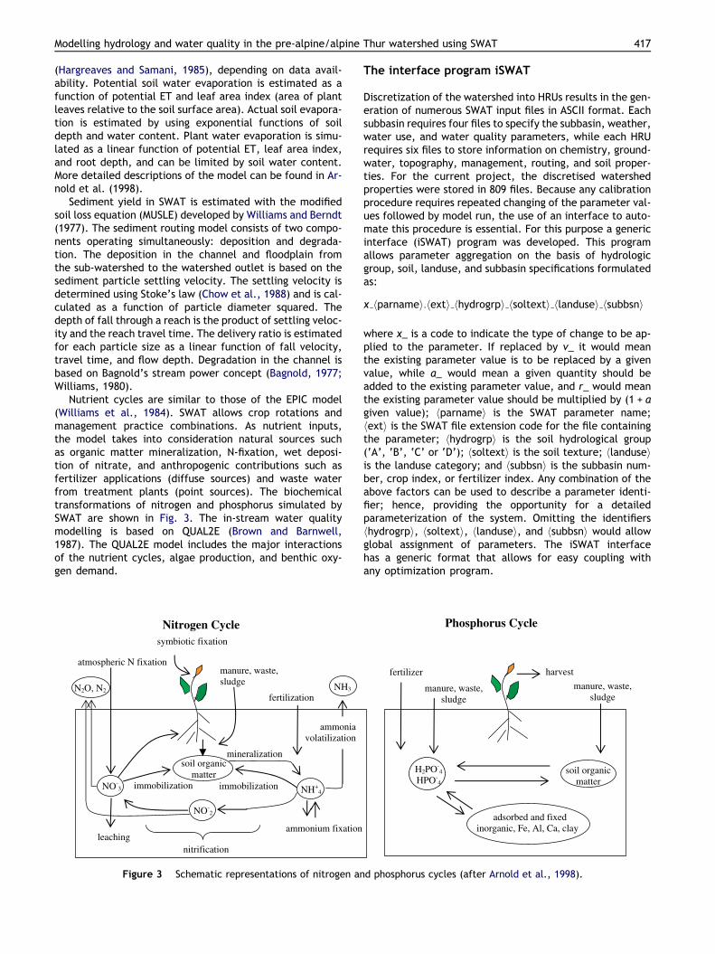
Nutrient cycles are similar to those of the EPIC model(Williams et al., 1984). SWAT allows crop rotations andmanagement practice combinations. As nutrient inputs,the model takes into consideration natural sources suchas organic matter mineralization, N-fixation, wet deposi-tion of nitrate, and anthropogenic contributions such asfertilizer applications (diffuse sources) and waste waterfrom treatment plants (point sources). The biochemicaltransformations of nitrogen and phosphorus simulated bySWAT are shown in Fig. 3. The in-stream water qualitymodelling is based on QUAL2E (Brown and Barnwell,1987). The QUAL2E model includes the major interactionsof the nutrient cycles, algae production, and benthic oxy-gen demand.
NH+4
NO-2
NO-3
leaching nitrification
soil organic matter
immobilization
mineralization
fertilization NH3
manure, waste, sludge
atmospheric N fixation
immobilization
symbiotic fixation
N2O, N2
Nitrogen Cycle
ammonia volatilization
ammonium fixation
Figure 3 Schematic representations of nitrogen an
The interface program iSWAT
Discretization of the watershed into HRUs results in the gen-eration of numerous SWAT input files in ASCII format. Eachsubbasin requires four files to specify the subbasin, weather,water use, and water quality parameters, while each HRUrequires six files to store information on chemistry, ground-water, topography, management, routing, and soil proper-ties. For the current project, the discretised watershedproperties were stored in 809 files. Because any calibrationprocedure requires repeated changing of the parameter val-ues followed by model run, the use of an interface to auto-mate this procedure is essential. For this purpose a genericinterface (iSWAT) program was developed. This programallows parameter aggregation on the basis of hydrologicgroup, soil, landuse, and subbasin specifications formulatedas:
x hparnamei:hexti hhydrogrpi hsoltexti hlandusei hsubbsni
where x_ is a code to indicate the type of change to be ap-plied to the parameter. If replaced by v_ it would meanthe existing parameter value is to be replaced by a givenvalue, while a_ would mean a given quantity should beadded to the existing parameter value, and r_ would meanthe existing parameter value should be multiplied by (1 + agiven value); hparnamei is the SWAT parameter name;hexti is the SWAT file extension code for the file containingthe parameter; hhydrogrpi is the soil hydrological group(‘A’, ‘B’, ‘C’ or ‘D’); hsoltexti is the soil texture; hlanduseiis the landuse category; and hsubbsni is the subbasin num-ber, crop index, or fertilizer index. Any combination of theabove factors can be used to describe a parameter identi-fier; hence, providing the opportunity for a detailedparameterization of the system. Omitting the identifiershhydrogrpi, hsoltexti, hlandusei, and hsubbsni would allowglobal assignment of parameters. The iSWAT interfacehas a generic format that allows for easy coupling withany optimization program.
adsorbed and fixed inorganic, Fe, Al, Ca, clay
H2PO-4
HPO-4
soil organic matter
manure, waste, sludge
harvest
manure, waste, sludge
fertilizer
Phosphorus Cycle
d phosphorus cycles (after Arnold et al., 1998).
418 K.C. Abbaspour et al.
In the current project iSWAT was coupled with SUFI-2optimization program (Abbaspour et al., 2004). A briefdescription of SUFI-2 is presented below.
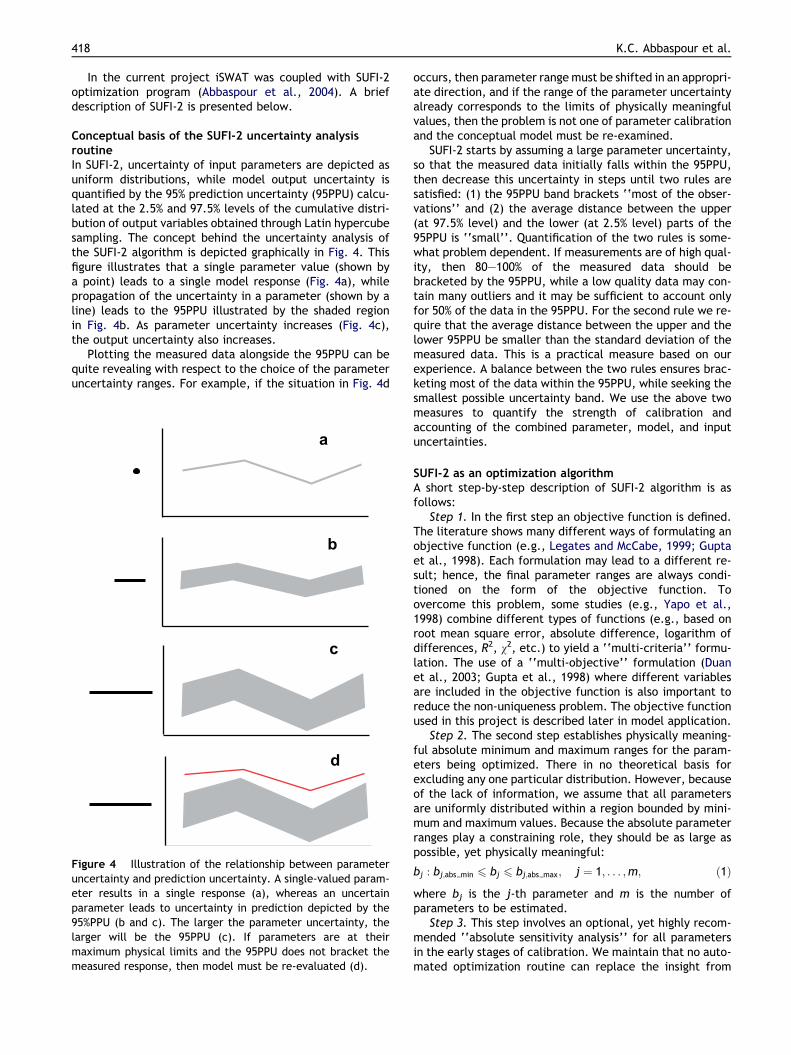
Conceptual basis of the SUFI-2 uncertainty analysisroutineIn SUFI-2, uncertainty of input parameters are depicted asuniform distributions, while model output uncertainty isquantified by the 95% prediction uncertainty (95PPU) calcu-lated at the 2.5% and 97.5% levels of the cumulative distri-bution of output variables obtained through Latin hypercubesampling. The concept behind the uncertainty analysis ofthe SUFI-2 algorithm is depicted graphically in Fig. 4. Thisfigure illustrates that a single parameter value (shown bya point) leads to a single model response (Fig. 4a), whilepropagation of the uncertainty in a parameter (shown by aline) leads to the 95PPU illustrated by the shaded regionin Fig. 4b. As parameter uncertainty increases (Fig. 4c),the output uncertainty also increases.
Plotting the measured data alongside the 95PPU can bequite revealing with respect to the choice of the parameteruncertainty ranges. For example, if the situation in Fig. 4d
a
b
c
d
Figure 4 Illustration of the relationship between parameteruncertainty and prediction uncertainty. A single-valued param-eter results in a single response (a), whereas an uncertainparameter leads to uncertainty in prediction depicted by the95%PPU (b and c). The larger the parameter uncertainty, thelarger will be the 95PPU (c). If parameters are at theirmaximum physical limits and the 95PPU does not bracket themeasured response, then model must be re-evaluated (d).
occurs, then parameter range must be shifted in an appropri-ate direction, and if the range of the parameter uncertaintyalready corresponds to the limits of physically meaningfulvalues, then the problem is not one of parameter calibrationand the conceptual model must be re-examined.
SUFI-2 starts by assuming a large parameter uncertainty,so that the measured data initially falls within the 95PPU,then decrease this uncertainty in steps until two rules aresatisfied: (1) the 95PPU band brackets ‘‘most of the obser-vations’’ and (2) the average distance between the upper(at 97.5% level) and the lower (at 2.5% level) parts of the95PPU is ‘‘small’’. Quantification of the two rules is some-what problem dependent. If measurements are of high qual-ity, then 80–100% of the measured data should bebracketed by the 95PPU, while a low quality data may con-tain many outliers and it may be sufficient to account onlyfor 50% of the data in the 95PPU. For the second rule we re-quire that the average distance between the upper and thelower 95PPU be smaller than the standard deviation of themeasured data. This is a practical measure based on ourexperience. A balance between the two rules ensures brac-keting most of the data within the 95PPU, while seeking thesmallest possible uncertainty band. We use the above twomeasures to quantify the strength of calibration andaccounting of the combined parameter, model, and inputuncertainties.
SUFI-2 as an optimization algorithmA short step-by-step description of SUFI-2 algorithm is asfollows:
Step 1. In the first step an objective function is defined.The literature shows many different ways of formulating anobjective function (e.g., Legates and McCabe, 1999; Guptaet al., 1998). Each formulation may lead to a different re-sult; hence, the final parameter ranges are always condi-tioned on the form of the objective function. Toovercome this problem, some studies (e.g., Yapo et al.,1998) combine different types of functions (e.g., based onroot mean square error, absolute difference, logarithm ofdifferences, R2, v2, etc.) to yield a ‘‘multi-criteria’’ formu-lation. The use of a ‘‘multi-objective’’ formulation (Duanet al., 2003; Gupta et al., 1998) where different variablesare included in the objective function is also important toreduce the non-uniqueness problem. The objective functionused in this project is described later in model application.
Step 2. The second step establishes physically meaning-ful absolute minimum and maximum ranges for the param-eters being optimized. There in no theoretical basis forexcluding any one particular distribution. However, becauseof the lack of information, we assume that all parametersare uniformly distributed within a region bounded by mini-mum and maximum values. Because the absolute parameterranges play a constraining role, they should be as large aspossible, yet physically meaningful:
where bj is the j-th parameter and m is the number ofparameters to be estimated.
Step 3. This step involves an optional, yet highly recom-mended ‘‘absolute sensitivity analysis’’ for all parametersin the early stages of calibration. We maintain that no auto-mated optimization routine can replace the insight from
X
Modelling hydrology and water quality in the pre-alpine/alpine Thur watershed using SWAT 419
physical understanding and knowledge of the effects ofparameters on the system response. The sensitivity analysisis carried out by keeping all parameters constant to realisticvalues, while varying each parameter within the range as-signed in step one. For each parameter about five simula-tions are performed by simply dividing the absolute rangesin equal intervals and allowing the midpoint of each intervalto represent that interval. Plotting results of these simula-tions along with the observations on the same graph givesinsight into the effects of the parameters on observedsignals.
Step 4. Initial uncertainty ranges are next assigned toparameters for the first round of Latin Hypercube sampling,i.e.
bj : ½bj;min 6 bj 6 bj;max�; j ¼ 1;m: ð2Þ
In general, the above ranges are smaller than the absoluteranges, are subjective, and are dependent upon experience.The sensitivity analysis in step 3 can provide a valuableguide for selecting appropriate ranges. Although important,these initial estimates are not crucial as they are updatedand allowed to change within the absolute ranges.
Step 5. A Latin Hypercube (McKay et al., 1979) samplingis carried out next; leading to n parameter combinations,where n is the number of desired simulations. This numbershould be relatively large (approximately 500–1000). Thesimulation program is then run n times and the simulatedoutput variable(s) of interest, corresponding to the mea-surements, are saved.
Step 6. As a first step in assessing the simulations, theobjective function, g, is calculated.
Step 7: In this step a series of measures is calculated toevaluate each sampling round. First, the sensitivity matrix,J, of g(b) is computed using:
Jij ¼DgiDbj
; i ¼ 1; . . . ;Cn2; j ¼ 1; . . . ;m; ð3Þ
where Cn2 is the number of rows in the sensitivity matrix
(equal to all possible combinations of two simulations),and j is the number of columns (number of parameters).Next, equivalent of a Hessian matrix, H, is calculated by fol-lowing the Gauss–Newton method and neglecting the high-er-order derivatives as:
H ¼ JTJ: ð4Þ
Based on the Cramer–Rao theorem (Press et al., 1992) anestimate of the lower bound of the parameter covariancematrix, C, is calculated from:
C ¼ s2gðJTJÞ�1; ð5Þ
where s2g is the variance of the objective function valuesresulting from the n runs. The estimated standard deviationand 95% confidence interval of a parameter bj is calculatedfrom the diagonal elements of C (Press et al., 1992) from:
where b�j is the parameter b for one of the best solutions(i.e. parameters which produce the smallest value of theobjective function), and m is the degrees of freedom
(n �m). Parameter correlations can then be assessed usingthe diagonal and off-diagonal terms of the covariance ma-trix as follows:
rij ¼Cijffiffiffiffiffiffi
Cii
p ffiffiffiffiffiffiCjj
p : ð9Þ
It is important to note that the correlation matrix r quan-tifies the change in the objective function as a result of achange in parameter i, relative to changes in the otherparameters j. As all parameters are allowed to change,the correlation between any two parameters is quitesmall.
Parameter sensitivities were calculated by calculatingthe following multiple regression system, which regressesthe Latin hypercube generated parameters against theobjective function values:
g ¼ aþXmi¼1
bibi: ð10Þ
A t-test is then used to identify the relative significance ofeach parameter bi. We emphasize that the measures of sen-sitivity given by [10] are different from the sensitivities cal-culated in step 3. The sensitivities given by [10] areestimates of the average changes in the objective functionresulting from changes in each parameter, while all otherparameters are changing. Therefore, [10] gives relative sen-sitivities based on linear approximations and, hence, onlyprovides partial information about the sensitivity of theobjective function to model parameters. Furthermore, therelative sensitivities of different parameters, as indicatedby the t-test, depend on the ranges of the parameters.Therefore, the ranking of sensitive parameters may changein every iteration.
Step 8. In this step measures assessing the uncertaintiesare calculated. Because SUFI-2 is a stochastic procedure,statistics such as percent error, R2, and Nash–Sutcliffe,which compare two signals, are not applicable. Instead,we calculate the 95% prediction uncertainties (95PPU) forall the variable(s) in the objective function. As previouslymentioned, this is calculated by the 2.5th (XL) and97.5th (XU) percentiles of the cumulative distribution ofevery simulated point. The goodness of fit is, therefore,assessed by the uncertainty measures calculated fromthe percentage of measured data bracketed by the95PPU band, and the average distance �d between theupper and the lower 95PPU (or the degree of uncertainty)determined from:
�dX ¼1
k
Xkl¼1ðXU � XLÞl; ð11Þ
where k is the number of observed data points. The bestoutcome is that 100% of the measurements are bracketedby the 95PPU, and �d is close to zero. However, because ofmeasurement errors and model uncertainties, the ideal val-ues will generally not be achieved. A reasonable measurefor �d, based on our experience, is calculated by the d-factorexpressed as:
d-factor ¼�dX
r; ð12Þ
420 K.C. Abbaspour et al.
where rX is the standard deviation of the measured variableX. A value of less than 1 is a desirable measure for thed-factor.
Step 9. Because parameter uncertainties are initiallylarge, the value of �d tends to be quite large during the firstsampling round. Hence, further sampling rounds are neededwith updated parameter ranges calculated from:
b0j;min ¼ bj;lower �maxðbj;lower � bj;minÞ
2;ðbj;max � bj;upperÞ
2
� �;
b0j;max ¼ bj;upper þ Maxðbj;lower � bj;minÞ
2;ðbj;max � bj;upperÞ
2
� �;
ð13Þ
where b 0 indicate updated values. The top p solutions areused to calculate bj,lower and bj,upper, and the largestðb0j;max � b0j;minÞ is used for the updated parameter range.The above criteria, while producing narrower parameterranges for each subsequent iteration, ensure that the up-dated parameter ranges are always centered on the top pcurrent best estimates, where p is a user defined value. Inthe final step, parameters are ranked according to their sen-sitivities, and highly correlated parameters are also identi-fied. Of the highly correlated parameters, those with thesmaller sensitivities should be fixed to their best estimatesand removed from additional sampling rounds.
Model parameterisation
In this study, the Thur watershed was subdivided into 16subbasins and 149 HRUs. The watershed parameterisationand the model input were derived using the SWAT ArcViewInterface (Di Luzio et al., 2002), which provides a graphicalsupport to the disaggregation scheme and allows the con-struction of the model input from digital maps. The basicdata sets required to develop the model input are: topogra-phy, soil, landuse and climatic data. The data used in mod-elling are as follows:
(i) Digital elevation model (DEM), produced by theswisstopo (grid cell: 25 m · 25 m) (DHM25@2004swiss-topo) (http://www.swisstopo.ch/en/products/digital/height/dhm25).
(ii) Digital stream network, produced by the swisstopo ata scale of 1:25,000 (Vector25@2004 swisstopo) (http://www.swisstopo.ch/en/products/digital/landscape/vec25/vec25gwn).
(iii) Soil map, produced by the Swiss Federal StatisticalOffice at a scale of 1:200,000 (BEK200, BFS Geostat,CH) (http://www.bfs.admin.ch/bfs/portal/en/index.html), and soil data from the Kanton Zurich Officeof Planning and Measurement (Bodenkarte 1:5000,ARV Kanton Zurich) (http://www.arv.zh.ch/).
(iv) Landuse map, produced by the Swiss Federal Statisti-cal Office (grid cell: 100 m · 100 m) (Arealstatistik1992/1997 BFS Geostat) (www.bfs.admin.ch).
(v) Agricultural census data, produced by Swiss FederalStatistical Office at a municipality level (www.bfs.admin.ch).
(vi) Climate data, records from 17 precipitation, eight airtemperature, five solar radiation, five relative humid-ity, and five wind speed gages over a period of 20
years (1980–2000) were used in the model, data wereobtained from the Swiss Federal Office of Meteorologyand Climatology (http://www.meteoschweiz.ch/web/en/weather.html).
(vii) Point source emissions include monthly organic nitro-gen, nitrates, nitrites and nitrogen ammonia dis-charges obtained from available records at severalcantonal stations for a period of 10 years (1991–2000) (Kanton Zurich, St. Gallen, Thurgau). All abovewebsites are active and have been last accessed onJune 2006.
The soil map includes 17 types of soils. Soil texture,available water content, hydraulic conductivity, bulk den-sity, and organic carbon content information were availablefor different layers (between two and five layers) for eachsoil type. A generalization of land management was thusestablished, considering five main classes: agriculture,range, forest-deciduous, forest-evergreen, urban, andwater. In the Thur watershed wheat occupied about 40%of crop areas, corn 20–25%, sugar beat 10–13% and potatoabout 5%. Representative crops for each subbasin/HRU wereselected according to the available cantonal agriculturalmanagement data. Wheat was chosen as a representativecrop in the lower portion of the Thur watershed, whereasthe middle and small fragments of the upper parts weredelineated as meadows.
In our simulation, the following management scheme wasadopted. Winter wheat was planted in mid-November, aftera tillage operation, followed by a fertilizer application of150 kg N ha�1 and 90 kg P ha�1. Winter wheat was harvestedin late August to early September and the soil was tilledagain, to incorporate plant residues. An average value of9 kg N ha�1 and 1 kg P ha�1 were applied on range grassesduring spring.
Available point source discharge records consisted ofmonthly values for the period of 1991–2000 on the subbasinlevel. Calculated average annual loads from available re-ported point sources were: 210 t year�1 for nitrates,360 t year�1 for total nitrogen and about 20 t year�1 for to-tal phosphorus.
An initial concentration of 1 ppm nitrogen was assumedin precipitation, but later this was calibrated to 1.3 ppm.Considering that the mean annual precipitation in the Thurbasin is 1460 mm, this corresponds to an average input ofabout 19 kg N ha�1 per year. This value is in agreement withdata given in the literature. The typical range of the totalnitrogen wet deposition for Switzerland is between 10 and20 kg N ha�1 per year (EAWAG News Information Bulletin,2000).
Model application
SWAT was calibrated based on the biweekly measured dis-charge, sediment, nitrate, and total phosphorous loads atthe watershed outlet at Andelfingen station (Fig. 2). Waterdischarge was measured continuously. Concentrations ofsediments (suspended solids), nitrate, and total phospho-rous in the river water were determined in biweekly com-posite flow proportional samples. Corresponding biweeklyloads were calculated as the product of biweekly averagewater discharge times concentration.
Modelling hydrology and water quality in the pre-alpine/alpine Thur watershed using SWAT 421
A constrained objective function was used to ensure cor-rect loads were being simulated for different landuses. Theobjective function, g, and the constraints were formulatedas follows:
Minimize :
g ¼ 1
r2Qm
X130i¼1ðQm � Q sÞ2i þ
1
r2Sm
X130i¼1ðSm � SsÞ2i
þ 1
r2Nm
X130i¼1ðNm � NsÞ2i þ
1
r2Pm
X130i¼1ðPm � PsÞ2i
Table 1 List of SWAT’s parameters that were fitted and their fin
Variable Sensitive parameter
Parameters sensitive to all four variables – snowfall tempera– Melt factor for sn– Melt factor for sn– Snowmelt base te– Snowmelt temper– Baseflow alpha fa– Groundwater dela– Curve number, r_– Manning’s n value– Effective hyd. con– Soil available wat– Soil hydraulic con– Soil bulk density,– Maximum canopy– Maximum canopy– Maximum canopy
Parameters sensitive to sediment only – Sediment routing– Channel re-entrai– Channel re-entrai– Channel erodabili– Channel cover fac
Parameters sensitive to totalphosphorus only
– Phosphorus availa– P enrichment rati– Rate constant for– Organic P settling
Parameters sensitive to nitrate only – Nitrogen in rain, R– Nitrogen uptake d– Concentration of– Organic N enrichm– Nitrate percolatio
Parameters sensitive to sedimentand total phosphorus
– support practice f– water erosion fac– water erosion fac– water erosion fac– soil erodability fa
a The extension (.bsn) refers to the SWAT file type where the paramb The fixed values indicate that a parameter was fitted and then fixec The qualifier (v__) refers to the substitution of a parameter by a va
the parameter were the current values is multiplied by 1 plus a factod AGRR = agricultural, PAST = pasture, ORCD = orchard, FRST = forest
6 PPasture 6 1:2 ðkg P ha�1Þ ð14Þwhere Q is the average biweekly discharge (m3 s�1), S is thetotal biweekly sediment load in the river (t), N is the totalbiweekly nitrate (NO3-N) load in the river (kg), P is the total
al calibrated values
s Final parametervalue
ture, SFTMP.bsna �1.1bow on December 21, SMFMN.bsn 0.36ow on June 21, SMFMX.bsn 2.84mperature, SMTMP.bsn 2.8ature lag factor, TIMP.bsn 0.29ctor, v__ALPHA_BF.gwc [0.17,0.34]y time, v__GW_DELAY.gw 0.74_CN2.mgt [0.085,0.045]for the main channel, v__CH_N2.rte [0.0,0.3]d. in the main channel, v__CH_K2.rte [4,14]er storage capacity, r__SOL_AWC.sol [�0.17,0.3]ductivity, r__SOL_K.sol [�0.19,0.5]r__SOL_BD.sol [�0.02.7,0.3]storage, v__CANMX.hru__AGRRd 2.8storage, v__CANMX.hru__FRST 4.8storage, v__CANMX.hru__PAST 4.1
factor in main channels, v__PRF.bsn [0.2,0.25]ned exponent parameter v__SPEXP.bsn [1.35,1.47]ned linear parameter v__SPCON.bsn [0.001,0.002]ty factor, v__CH_EROD.rte [0.12,0.14]tor, v__CH_COV.rte [0.2,0.25]
bility index, v__PSP.bsn [0.5,0.7]o with sediment loading, ERORGP.hru [2.0,4.0]mineralization of organic P, BC4.swq [0.3,0.5]rate, RS5.swq [0.08,0.1]
CN.bsn 1.3istribution parameter, UBN.bsn 9.4NO3 in groundwater, r__GWNO3.gw [�0.3,0.5]ent for sediment, ERORGN.hru 2.75n coefficient, NPERCO.bsn 0.223
actor r__USLE_P.mgt [�0.6,�0.1]tor v__USLE_C.crp____AGRR [0.03,0.3]tor v__USLE_C.crp____PAST,ORCD [0.07,0.2]tor v__USLE_C.crp____FRST [0.0,0.1]ctor, r__USLE_K.sol [�0.19,0.5]eter occurs.d.lue from the given range, while (r__) refers to a relative change inr in the given range..
422 K.C. Abbaspour et al.
biweekly total phosphorus load (kg), r2 is the variance, and‘m’ and ‘s’ subscripts stand for measured and simulated,respectively. In the constraints, SLanduse is the average an-nual sediment load of the landuse in the watershed (t ha�1),NLanduse is the average annual nitrate load of the landuse(kg N ha�1), and PLanduse is the average annual total phos-phorus load of the landuse (kg P ha�1) all in the period of
Discharge C
0
100
200
300
400
500
600
700
01.01.91 01.07.91 01.01.92 01.07.92 01.01.93 01.
D
Dai
ly d
isch
arge
(m
3 s-
1 )
measured data bracketed by the 95PPU = 91%
d-factor = 1.0
Discharge V
0
100
200
300
400
500
600
700
800
900
1000
01.01.96 01.07.96 01.01.97 01.07.97 01.01.98 01
D
Dai
ly d
isch
arge
(m
3 s-
1 )
measured data bracketed by the 95PPU = 89%
d-factor = 0.95
95PPU
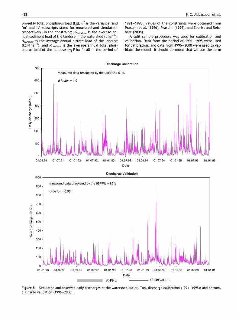
Figure 5 Simulated and observed daily discharges at the watershedischarge validation (1996–2000).
1991–1995. Values of the constraints were obtained fromPrasuhn et al. (1996), Prasuhn (1999), and Zobrist and Reic-hert (2006).
A split sample procedure was used for calibration andvalidation. Data from the period of 1991–1995 were usedfor calibration, and data from 1996–2000 were used to val-idate the model. It should be noted that we use the term
d outlet. Top, discharge calibration (1991–1995); and bottom,
Modelling hydrology and water quality in the pre-alpine/alpine Thur watershed using SWAT 423
‘‘validation’’ to comply with the traditional literature syn-tax. We are well aware that a watershed model can neverbe fully validated.
Results and discussion
Calibration of models at a watershed scale is a challengingtask because of the possible uncertainties that may exist inthe form of process simplification, processes not accountedfor by the model, and processes in the watershed that areunknown to the modeller. Some examples of the abovementioned model uncertainties are: effects of wetlandsand reservoirs on hydrology and chemical transport; inter-action between surface and groundwater; occurrences oflandslides, and large constructions (e.g., roads, dams, tun-
0
300
600
900
1200
01.01.1999 01.04.1999 01.07.1Dat
Dai
ly d
isch
arge
(m
3 s-1
)
Wet Year 1999
measured data bracketed by the 95PPU =d-factor = 0.74
0
300
600
900
1200
01.01.2000 01.04.2000 01.07.2Date
Dai
ly d
isch
arge
(m
3 s-1
) Average Year (2000)
measured data bracketed by the 95PPU d-factor = 1.20
0
300
600
900
1200
01.01.1997 01.04.1997 01.07.1Date
Dai
ly D
isch
arge
(m
3 s-1
)
Dry Year 1997
measured data bracketed by the 95PPU d-factor = 1.13
Figure 6 Breakdown of simulated daily dis
nels, bridges) that could produce large amounts of sedi-ments for a number of years affecting water quantity andquality; unknown wastewater discharges into water streamsfrom factories and water treatment plants; and unac-counted for fertilization, irrigation and water diversions,and other activities in the river flood planes such as agricul-tural activities and dumping of construction materials. In aseparate project in the Chaohe Basin in North China, weexperienced insurmountable difficulties with simulation ofsediment load in the river because of activities such as con-struction, material dumping, etc. The Thur watershed,however, during the period of study was relatively free ofsuch activities; hence, model uncertainties were limitedto the errors in the process simplifications alone, e.g.,the simplification in the universal soil loss equation usedin SWAT.
999 01.10.1999 01.01.2000e
90%
000 01.10.2000 01.01.2001
= 90%
997 01.10.1997 01.01.1998
= 91%
charge into wet, average, and dry years.
424 K.C. Abbaspour et al.
Further sources of uncertainties in distributed modelsare due to inputs such as rainfall and temperature. Rainfalland temperature data are measured at local stations andregionalization of these data may introduce large errors,especially in mountainous regions. If an anomalous site isused, then runoff results may be skewed high or low. InSWAT, climate data for every subbasin is furnished by thestation nearest to the centroid of the subbasin. Directaccounting of rainfall or temperature distribution error isquite difficult as information from many stations would berequired. But the ‘‘elevation band’’ option in SWAT couldto some extent alleviate this error by adjusting the temper-ature and rainfall to account for orographic effects of asubbasin.
Given the above possible errors, calibration and valida-tion results of the Thur watershed could be qualified as‘‘excellent’’ in this study. This indicates a good quality ofthe input data as well as small conceptual model errors inthe dominant processes in the watershed.
We began the calibration process by initially includingsome 50 parameters in the SUFI-2 algorithm, but in the fifthand last iteration only 30 were found to be sensitive to dis-charge, sediment, nitrate, and total phosphorus. In eachiteration, 1000 model calls were performed, for a total of5000 simulations, attesting the efficiency of SUFI-2. An‘‘absolute sensitivity analysis’’ (changing the parametersone at a time while keeping other parameters constant)was performed for all 50 parameters after the second itera-tion. The response of all four variables to changes in eachparameter was plotted. This helped to identify the insensi-tive parameters (causing no or very small changes to vari-ables), the sensitive parameters to all four variables, andthe parameters that were sensitive to sediment only, totalphosphorus only, and nitrate only (Table 1). This informationproved to be quite useful in operating SUFI-2, which is a par-tially automated procedure requiring the analyst’s attentionin parameter updating at the end of each iteration.
It is worth mentioning that the results of the absoluteand relative sensitivity analysis conducted for the Thur wa-
Table 2 Break down of water fluxes and sediment and nutrient lwet, and an average year
FRST = forest, AGRR = agricultural, PAST = summer pasture, ET = evastream, GWQ = groundwater contribution to stream flow, WYLD = SURQroot zone (groundwater recharge), SYLD = sediment yield, TN = total na All entries are averages for landuses occurring in different subbasi
tershed may not be directly applicable to other sites. In thefirst procedure all parameters except one are kept constant;hence, the sensitivity of the varying parameter is condi-tional upon the values of all others. While in the later case,the sensitivity of parameters depends on the ranges that areassigned to the parameters. As the values of the fixedparameters or the ranges change, the sensitivity of theparameters may also change. Hence, such analysis mustbe performed for each site locally.
Other important considerations in the calibration of thepre-alpine/alpine Thur watershed were the corrections ap-plied through the use of ‘‘elevation band’’ option in SWAT.We assigned four elevation bands with centers at 612, 115,1691, and 2230 m for the subbasins 2, 5, 8, 9, 11, and 15 lo-cated at higher elevations (Fig. 2). The lapse rates of1 mm km�1 and �6 �C km�1 were applied to rainfall andtemperature, respectively. The use of elevation band wasnecessary to correct a shift in the discharge data and theoverall dynamics of flow. The calibrated snow-relatedparameters are given in Table 1.
The results of the daily discharge simulation are shown inFig. 5. These simulations are based on a calibration thatused biweekly discharge, sediment, nitrate, and total phos-phorus in the objective function. The calibration and valida-tion statistics are also given in the figures for ease ofreferencing. The shaded region (95PPU), which is the simu-lation result, quantifies all uncertainties because it bracketsa large amount of the measured data, which contains alluncertainties. The parameter ranges leading to the 95PPUare also given in Table 1. In SUFI-2, parameter uncertaintyaccounts for all sources of uncertainty, e.g., input uncer-tainty, conceptual model uncertainty, and parameteruncertainty, because disaggregation of the error into itssource components is difficult, particularly in cases commonto hydrology where the model is nonlinear and differentsources of error may interact to produce the measured devi-ation (Gupta et al., 2005).
In discharge calibration, 91% of the measured data werebracketed by the 95PPU while the d-factor had a desired va-
oads into different components for major landuses for a dry, a
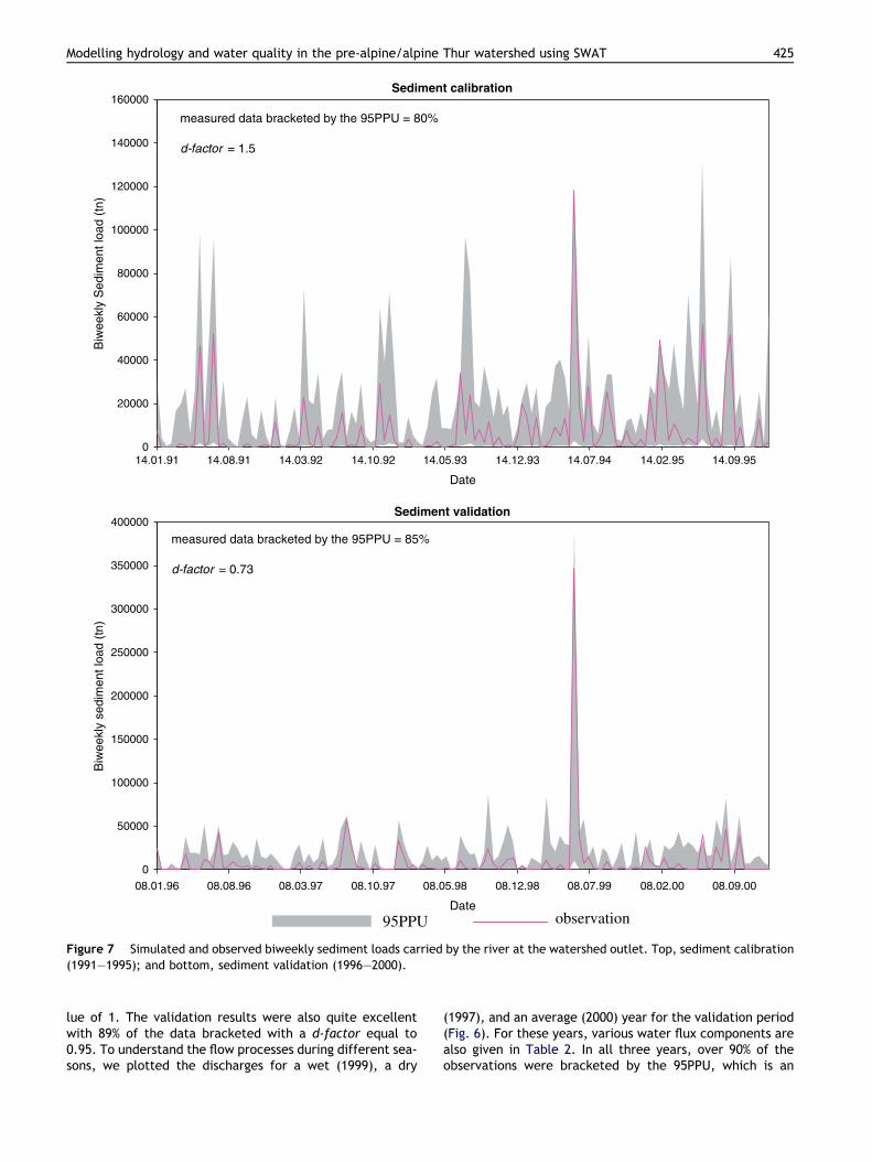
Figure 7 Simulated and observed biweekly sediment loads carried by the river at the watershed outlet. Top, sediment calibration(1991–1995); and bottom, sediment validation (1996–2000).
Modelling hydrology and water quality in the pre-alpine/alpine Thur watershed using SWAT 425
lue of 1. The validation results were also quite excellentwith 89% of the data bracketed with a d-factor equal to0.95. To understand the flow processes during different sea-sons, we plotted the discharges for a wet (1999), a dry
(1997), and an average (2000) year for the validation period(Fig. 6). For these years, various water flux components arealso given in Table 2. In all three years, over 90% of theobservations were bracketed by the 95PPU, which is an
426 K.C. Abbaspour et al.
excellent statistic. The dry and average years, however,have slightly larger prediction uncertainties associated withthem. It should be noticed that the use of the term ‘‘dry’’ isrelative as the rainfall is still greater than 1077 mm. Thefluxes in Table 2 reveal that in an average or a wet year sur-face runoff dominates water yield. In a dry year, however,lateral flow contribution makes up a larger part of the wateryield from the landuses. Perhaps one important reason forthe favourable discharge simulation of the Thur watershedis the fact that most of the rainfall in the region translatesinto runoff and lateral flow, and parameters dealing withthe lesser understood processes such as groundwater re-charge, and groundwater–river interaction were not asimportant as they would have been if surface runoff and lat-eral flow did not dominate the flow processes.
The results for biweekly sediment are shown in Fig. 7.About 80% of the data were bracketed by the 95PPU andthe d-factor had a value of 1.5. Most of the data missingthe 95PPU band were from the very small sediment loads,while all of the peaks were accounted for. The calibrationand validation statistics show larger uncertainties than dis-charge. In the validation, 85% of the data were bracketed bythe 95PPU, although the d-factor is small – primarily due toone large observation resulting in a large standard devia-tion. Removing this observation gives a larger value of 1.4for the d-factor. A common problem in the prediction ofparticulates such as sediment and organic phosphorus is thatof the ‘‘second-storm’’ effect. After a storm, there is lesssediment to be moved, and the remaining surface layer ismuch more difficult to mobilize. Hence, a similar sizestorm, or even a bigger size second or third storm could
sediment "s
0
5000
10000
15000
20000
25000
30000
35000
13.09.92 03.10.92 23.10.92 12.11.92
Dat
Sed
imen
t (tn
)
Obs. sediment Sim. sediment
Obs. discharge
storm 1
storm 2
Figure 8 Illustration of the ‘‘second-storm’’ effect on sediment.does not account for this phenomenon, hence, overestimating the
actually result in smaller sediment loads. The model, how-ever, does not account for this effect as illustrated inFig. 8. The model produces a good simulation of sedimentload for the first storm, while in the second and the thirdstorms it overestimated the load.
Five parameters were found to be sensitive to sedimentonly. These included sediment routing factor in the mainchannels (PRF.bsn), channel re-entrained exponent parame-ter (SPEXP.bsn), channel re-entrained linear parameter(SPCON.bsn), channel erodability factor (CH_EROD.rte),and channel cover factor (CH_COV.rte). Three other param-eters were found to be sensitive to both sediment and totalphosphorus. These included support practice factor (US-LE_P.mgt), water erosion factor (USLE_C.crp), and soil ero-dability factor (USLE_K.sol). Fourteen other dischargerelated parameters listed in Table 1 were also sensitive tosediment.
Results of the total phosphorus (TP) simulation in the riv-er discharge are shown in Fig. 9. As a large part of TP is theorganic component transported by sediment, the ‘‘second-storm’’ effect as described for the sediment also appliesto TP. For this reason the uncertainty in TP is also large asindicated by a d-factor of 1.35 for calibration while bracket-ing only 78% of the data. As in the sediment, the validationd-factor would also have been quite large without the largeobservation occurring in the June of 1999 where a large TPload of 478,054 kg was reported.
Four parameters were found to be sensitive to TP only(Table 1). These included phosphorus availability index(PSP.bsn), P enrichment ratio with sediment loading (ERO-RGP.hru), rate constant for mineralization of organic P
econd-storm" effect
02.12.92 22.12.92 11.01.93 31.01.93
e
0
20
40
60
80
100
120
140
160
Dis
char
ge (
m3
s-1 )
After a storm there is less sediment to be carried. The modelobservation.
Figure 9 Simulated and observed biweekly total phosphorus loads carried by the river at the watershed outlet. Top, totalphosphorus calibration (1991–1995); and bottom, total phosphorus validation (1996–2000).
Modelling hydrology and water quality in the pre-alpine/alpine Thur watershed using SWAT 427
(BC4.swq), and organic P settling rate (RS5.swq). The lasttwo of these parameters are related to in-streamprocesses.
Results of the nitrate simulation are given in Fig. 10. Similarto the discharge, the nitrate simulation is also very good withsmall uncertainties, d-factor = 1, while bracketing 82% of the
428 K.C. Abbaspour et al.
data for calibration and 84% for validation. Five parameterswere found to be sensitive to nitrate only. These includednitrogen in rain (RCN.bsn), nitrogen uptake distribution
Nitrate
0
200000
400000
600000
800000
1000000
1200000
14.01.91 14.08.91 14.03.92 14.10.92 14.
Biw
eekl
y ni
trat
e (k
g)
measured data bracketed by the 95PPU = 82%
d-factor = 1.0
Nitrate
0
200000
400000
600000
800000
1000000
1200000
1400000
1600000
08.01.96 08.08.96 08.03.97 08.10.97 08.
Biw
eekl
y N
itrat
e lo
ad (
kg)
measured data bracketed by the 95PPU = 84%
d-factor = 1.0
95PPU
Figure 10 Simulated and observed biweekly nitrate loads carried(1991–1995); and bottom, nitrate validation (1996–2000).
parameter (UBN.bsn), concentration of nitrate in groundwater(GWNO3.gw), organic N enrichment for sediment (ERO-RGN.hru), and nitrate percolation coefficient (NPERCO.bsn).
calibration
05.93 14.12.93 14.07.94 14.02.95 14.09.95
Date
validation
05.98 08.12.98 08.07.99 08.02.00 08.09.00
Date
observation
by the river at the watershed outlet. Top, nitrate calibration
Modelling hydrology and water quality in the pre-alpine/alpine Thur watershed using SWAT 429
In Table 2, sediment and nutrient loads released formthe major landuses into the river is also reported for awet, a dry, and an average year. As expected, the largestloads are produced in the wet year from the agriculturallanduse followed by the summer pasture.
Two points are worth mentioning here. First, the objec-tive function contained four variables, calibrating the mod-el for any one variable would produce much better resultsfor that variable but would not give as good a simulation re-sult for other variables (the conditionality problem, Abbas-pour et al., 1999). Second, ignoring the constraints wouldalso produce better calibration and validation results atthe watershed outlet, but the simulated loads from variouslanduses would not comply with our previous knowledge.Both these points indicate the importance of adding morevariables in and constraining the objective function. Thisproduces parameters reflecting more of the local processes,hence, providing more reasonable simulations. The downside is that more data are required for a reliable model cal-ibration at the watershed scale. This also raises the impor-tant questions: when is a watershed model calibrated? Andfor what purpose can it be used for?
Conclusions
Given the complexities of a watershed and the large numberof interactive processes taking place simultaneously andconsecutively at different times and places within a wa-tershed, it is quite remarkable that the simulated resultscomply with the measurements to the degree that theydo. Based on the results obtained in this study, SWAT is as-sessed to be a reasonable model to use for water quality andwater quantity studies in the Thur watershed. On that posi-tive note, however, a careful calibration and uncertaintyanalysis and proper application of modelling results shouldbe exercised. The following conclusions could be drawnfrom the present study:
1. A watershed model calibrated based on measured data atthe outlet of the watershed may produce erroneousresults for various landuses and subbasins within thewatershed, unless the objective function was con-strained to produce correct results. This means that alarge amount of measured data are necessary for aproper model calibration.
2. Simulation of particulates such as sediment and phospho-rus are subject to large model uncertainties because ofthe ‘‘second-storm’’ effect, among others.
3. Large-scale watershed models could be effective for sim-ulating watershed processes and therefore watershedmanagement studies. The simulation of hydrology, sedi-ment, and nutrient loads were of reasonable accuracy,allowing such integrated models to be used in scenarioanalysis.
Acknowledgments
This study is a part of the NADUF program and supported bythe Swiss Federal Office for Environment (FOEN), the Swiss
Federal Institute of Aquatic Science and Technology (Ea-wag), and MeteoSwiss. Special thanks to the graduate stu-dents at Eawag for their valuable contribution incollecting and processing environmental data.
References
Abbaspour, K.C., van Genuchten, M. Th., Schulin, R., Schlappi, E.,1997. A sequential uncertainty domain inverse procedure forestimating subsurface flow and transport parameters. WaterResour. Res. 33, 1879–1892.
Abbaspour, K.C., Sonnleitner, M., Schulin, R., 1999. Uncertainty inestimation of soil hydraulic parameters by inverse modeling:example Lysimeter experiments. Soil Sci. Soc. Am. J. 63, 501–509.
Abbaspour, K.C., Johnson, A., van Genuchten, M.Th., 2004.Estimating uncertain flow and transport parameters using asequential uncertainty fitting procedure. Vadose Zone J. 3,1340–1352.
Arnold, J.G., Srinisvan, R., Muttiah, R.S., Williams, J.R., 1998.Large area hydrologic modeling and assessment. Part I: modeldevelopment. J. Am. Water Resour. Assoc. 34 (1), 73–89.
Bagnold, R.A., 1977. Bedload transport in natural rivers. WaterResour. Res. 13 (2), 303–312.
Beven, K., Binley, A., 1992. The future of distributed models: modelcalibration and uncertainty prediction. Hydrol. Process. 6, 279–298.
Di Luzio, M., Srinisvasan, R., Arnold, J.G., Neitsch, S.L., 2002.ArcView Interface for SWAT2000, Blackland Research & Exten-sion Center, Texas Agricultural Experiment Station and Grass-land, Soil and Water Research Laboratory, USDA AgriculturalResearch Service.
Duan, Q., Sorooshian, S., Gupta, H.V., Rousseau, A.N., Turcotte,R., 2003. Calibration of Watershed Models. American Geophys-ical Union, Washington, DC.
EAWAG News Information Bulletin, 2000. Ground Water Research inPractice, No. 49, EAWAG, Duebendorf, Switzerland.
Ewen, J., Parkin, G., O’Connell, E., 2000. SHETRAN: distributedbasin flow and transport modelling system. J. Hydrol. Eng. 5 (3),250–258.
Gupta, H.V., Sorooshian, S., Yapo, P.O., 1998. Toward improvedcalibration of hydrologic models: multiple and noncommensu-rable measures of information. Water Resour. Res. 34, 751–763.
Gupta, H.V., Sorooshian, S., Hogue, T.S., Boyle, D.P., 2003.Advances in automated calibration of watershed models. In:Duan, Q., Gupta, H.V., Sorooshian, S., Rousseau, A.N., Turcotte,R. (Eds.), Calibration of Watershed Models. American Geophys-ical Union, Washington, DC.
430 K.C. Abbaspour et al.
Gupta, H.V., Beven, K.J., Wagener, T., 2005. Model calibration anduncertainty estimation. In: Anderson, M.G. (Ed.), Encyclopediaof Hydrological Sciences. Wiley, New York, pp. 2015–2031.
Gurtz, J., Baltensweiler, A., Lang, H., 1999. Spatially distributedhydrotope-based modelling of evapotranspiration and runoff inmountainous basins. Hydrol. Process. 13, 2751–2768.
Huber, W.C., 1993. Contaminant transport in surface water. In:Maidment, D.R. (Ed.), Handbook of Hydrology. McGraw-Hill,New York, pp. 14.1–14.50.
Jakob, A., Binderheim-Bankay, E., Davis, J.S., 2002. National long-term surveillance of Swiss Rivers. Verh. Internat. Verein. Limnol.28, 1101–1106.
Legates, D.R., McCabe, G.J., 1999. Evaluating the use of ‘‘good-ness-of-fit’’ measures in hydrologic and hydroclimatic modelvalidation. Water Resour. Res. 35, 233–241.
McKay, M.D., Beckman, R.J., Conover, W.J., 1979. A comparison ofthree methods for selecting values of input variables in theanalysis of output from a computer code. Technometrics 21,239–245.
Monteith, J.L., 1965. Evaporation and environment. In: Fogg, G.F.(Ed.), The State and Movement of Water in Living Organisms.Cambridge University Press, Cambridge, pp. 205–234.
Prasuhn, V., 1999. Phosphor und Stickstoff aus diffusen Quellen imEinzugsgebiet des Bodensees, Ber. Int. Gewasserschutzkomm.Bodensee: V.51, Eidg. Forschungsanstalt fur Agrarokologie undLandbau (FAL), Intstitut fur Umweltschutz und Landwirtschaft(IUL) (report in German).
Prasuhn, V., Sieber, U., 2005. Changes in diffuse phosphorus andnitrogen inputs into surface waters in the Rhine watershed inSwitzerland. Aquat. Sci. 67 (3), 363–371.
Prasuhn, V., Spiess, E., Braun, M., 1996. Methoden zur Abschatzungder Phosphor’und Stickstofeintrage aus diffusen Quellen in denBodensee, Ber. Int. Gewasserschutzkomm. Bodensee: V.45,Institut fur Umweltschutz und Landwirtschaft (IUL) (report inGerman).
Press, W.H., Flannery, B.P., Teukolsky, S.A., Vetterling, W.T.,1992. Numerical Recipe: The Art of Scientific Computation,second ed. Cambridge University Press, Cambridge.
Priestley, C.H.B., Taylor, R.J., 1972. On the assessment of surfaceheat flux and evaporation using large-scale parameters. MonthlyWeather Rev. 100, 81–92.
SAEFL (Swiss Agency for the Environment, Forests and Land-scapes) (SAEFL), 2002. Environment – Switzerland 2002report, vol. 1.
Simunek, J., Wendroth, O., van Genuchten, M.Th., 1999. Estimat-ing unsaturated soil hydraulic properties from laboratory tensiondisc infiltrometer experiments. Water Resour. Res. 35, 2965–2979.
Singh, J., Knapp, H.V., Arnold, J.G., Demissie, M., 2005.Hydrological modeling of the Iroquois river watershedusing HSPF and SWAT. J. Am. Water Resour. Assoc. 41(2), 343–360.
Thornthwaite, C.W., 1948. An approach toward a rational classifi-cation of climate. Geogr. Rev. 38, 55–94.
Wang, W., Neuman, S.P., Yao, T., Wierenga, P.J., 2003. Simulationof large-scale field infiltration experiments using a hierarchy ofmodels based on public, generic, and site data. Vadose Zone J.2, 297–312.
Williams, J.R., 1980. SPNM, a model for predicting sediment,phosphorous, and nitrogen from agricultural basins. WaterResour. Bull. 16 (5), 843–848.