Monetary Policy and the Redistribution Channel*

Adrien Auclert†

December 2018

Abstract

This paper evaluates the role of redistribution in the transmission mechanism ofmonetary policy to consumption. Three channels affect aggregate spending whenwinners and losers have different marginal propensities to consume: an earningsheterogeneity channel from unequal income gains, a Fisher channel from unexpectedinflation, and an interest rate exposure channel from real interest rate changes. Suffi-cient statistics from Italian and U.S. data suggest that all three channels are likely toamplify the effects of monetary policy.

JEL Classification: D31, D52, E21, E52.

*This paper is a revised version of Chapter 1 of my PhD dissertation at MIT. I cannot find enough words to thankmy advisors Iván Werning, Robert Townsend and Jonathan Parker for their continuous guidance and support. Ialso thank many seminar participants for their insights. I have particularly benefited from the detailed commentsof the editor (John Leahy), four anonymous referees, as well as Eduardo Dávila, Gauti Eggertsson, Xavier Gabaix,Adam Guren, Gregor Jarosch, Greg Kaplan, Guido Lorenzoni, Ben Moll, Makoto Nakajima, Matthew Rognlie,Yoko Shibuya, Alp Simsek, Christian Stoltenberg, Daan Struyven and Tetti Tzamourani. Filippo Pallotti providedoutstanding research assistance, and the Macro-Financial Modeling Group provided generous financial support.

†Stanford University and NBER. Email: aauclert@stanford.edu.

There is a conventional view that redistribution is a side effect of monetary policychanges, separate from the issue of aggregate stabilization which these changes aim toachieve. Most models of the monetary policy transmission mechanism implicitly adoptthis view by featuring a representative agent. By contrast, in this paper I argue that re-distribution is a channel through which monetary policy affects macroeconomic aggre-gates, because those who gain from accommodative monetary policy have higher marginalpropensities to consume (MPCs) than those who lose. The simple argument goes back toTobin (1982):

Aggregation would not matter if we could be sure that the marginal propensities to spendfrom wealth were the same for creditors and for debtors. But [...] the population is not dis-tributed between debtors and creditors randomly. Debtors have borrowed for good reasons,most of which indicate a high marginal propensity to spend from wealth or from currentincome.

In this paper, I use consumer theory to refine Tobin’s intuitions about aggregation. Myanalysis clarifies who gains and who loses from monetary policy changes, as well as theeffect on aggregate consumption. Monetary expansions tend to increase real incomes, toraise inflation and to lower real interest rates. Not everyone is equally affected by thesechanges. This generates three distinct sources of redistribution.

First, monetary expansions increase labor and profit earnings. The distribution of thesegains is unlikely to be equal: some agents tend to benefit disproportionately, and con-versely, some tend to lose in relative terms. This is the earnings heterogeneity channel ofmonetary policy.

Second, unexpected inflation revalues nominal balance sheets, with nominal creditorslosing and nominal debtors gaining: this is the Fisher channel, which has a long history inthe literature since Fisher (1933). This channel has been explored by Doepke and Schneider(2006), who measure the balance sheet exposures of various sectors and groups of house-holds in the United States to different inflation scenarios. Net nominal positions (NNPs)quantify the exposures to unexpected increases in the price level.

Real interest rate falls create a third, more subtle form of redistribution. These fallsincrease financial asset prices. But it is incorrect to claim that asset holders generally ben-efit: instead, we have to consider whether their assets have longer durations than theirliabilities. Importantly, liabilities include consumption plans, and assets include humancapital. Unhedged interest rate exposures (UREs)—the difference between all maturingassets and liabilities at a point in time—are the correct measure of households’ balance-sheet exposures to real interest rate changes, just like net nominal positions are for pricelevel changes. For example, agents whose financial wealth is primarily invested in short-term certificates of deposit tend to have positive UREs, while those with large long-term

1

bond investments or adjustable-rate mortgage liabilities tend to have negative UREs. Realinterest rate falls redistribute away from the first group towards the second group: this iswhat I call the interest rate exposure channel.

In this paper, I show how these three redistribution channels affect the transmissionmechanism of monetary policy to consumption. My main theoretical result decomposesthe consumption effect of a transitory change in monetary policy into a contribution fromeach of these channels, together with an aggregate income and a substitution channel. Repre-sentative-agent models only feature the latter two. My theorem shows that redistribu-tion amplifies these effects, provided that winners from monetary expansions have higherMPCs than losers. The rest of the paper argues that this appears to be the case in thedata. In brief, the redistributive effects of monetary policy are important to understand itsaggregate effects.1

In the first part of the paper, I establish my main decomposition by studying a generalaggregation problem. In partial equilibrium, I consider an optimizing agent with a giveninitial balance sheet, who values nondurable consumption and leisure, and is subject toa transitory change in income, inflation and the real interest rate. I decompose his con-sumption response into a substitution effect and a wealth effect, and show that the latteris the product of his MPC out of income and a balance-sheet revaluation term in whichNNPs and UREs appear. This result is robust to the presence of durable goods, incompletemarkets, idiosyncratic risk, and (certain kinds of) borrowing constraints. In other words,the MPC out of a windfall income transfer is a key determinant of the response of optimiz-ing consumers to inflation– or real interest rate–induced changes in their balance sheets.This result generalizes previous findings by Kimball (1990) on the importance of MPCs inincomplete-markets consumption models.

I then aggregate these individual-level predictions and exploit the fact that financialassets and liabilities net out in general equilibrium to obtain the first-order response ofaggregate consumption to simultaneous transitory shocks to output, inflation, and the realinterest rate. This response is the sum of five terms, reflecting the contributions from thetwo aggregate and the three redistributive channels mentioned above. Moreover, the mag-nitudes of the redistributive channels are given by sufficient statistics: the cross-sectionalcovariances between MPCs and exposures to each aggregate shock. Since the pioneeringwork of Harberger (1964), sufficient statistics have been used in public finance to evaluate

1My theorem applies to a broad class of general equilibrium models with heterogeneous agents, so it can beused to understand consumption in other contexts than that of monetary policy. At the same time, I am leaving anumber of redistributive channels out of my analysis. First, I abstract away from aggregate risk, so cannot handlechanges in risk premia, as in Brunnermeier and Sannikov (2016). Second, I do not model limited participation, somonetary policy cannot differentially affect participants and nonparticipants, as in the studies of Grossman andWeiss (1983), Rotemberg (1984) and others. Finally, since I assume that all assets are remunerated at the risk-freerate, my analysis does not address the unequal incidence of inflation due to larger cash holdings by the poor (Erosaand Ventura 2002; Albanesi 2007). These are all interesting dimensions along which the theory could be extended.

2

the welfare effect of hypothetical policy changes in a way that is robust to the specifics ofthe underlying structural model (see Chetty 2009 for a survey). Mine are useful to evaluatethe impact of hypothetical changes in macroeconomic aggregates on aggregate consumptionin a similarly robust way. All that is required is information on household balance sheets,income and consumption levels, and their MPCs.

By further assuming that the elasticity of intertemporal substitution σ and the elasticityof relative income to aggregate income γ are constant in the population, I obtain a set offive estimable moments that summarize all we need to know about agents’ heterogeneityto recover the aggregate elasticities of consumption to the real interest rate, the price level,and aggregate income. Contrary to σ (and perhaps γ), these sufficient statistics are notstructural parameters: they are likely to vary over time and across countries.2 I set out tomeasure them in three separate surveys, covering different time periods, countries, andmethods from the literature. I use a 2010 Italian survey containing a self-reported mea-sure of MPC (Jappelli and Pistaferri 2014); the 1999-2013 waves of the U.S. Panel Surveyof Income Dynamics, together with semi structural approach to identify the MPC out oftransitory income shocks (Blundell, Pistaferri and Preston 2008); and the 2001–2002 wavesof the U.S. Consumer Expenditure Survey, together with a method that exploits the ran-domized timing of tax rebates as a source of identification for MPC (Johnson, Parker andSouleles 2006).

Consider first the elasticity of consumption to the real interest rate. In a representative-agent world, this elasticity is due to intertemporal substitution. It is negative, and itsmagnitude depends on σ. I define a method for measuring UREs, and show that, in eachof my three datasets, their covariance with MPCs is also negative. Through the lens of mytheorem, this implies that the interest rate exposure channel acts in the same direction asthe substitution channel, and with comparable magnitude provided that σ is between 0.1and 0.4. Hence representative-agent analyses that abstract from redistribution may fail tocapture an important reason why real interest rates affect consumption, especially if σ issmall.3

Similarly, across datasets, the covariance between MPCs and NNPs is negative on av-erage. This implies that consumption tends to increase with inflation as a result of theFisher channel. However, when cast in terms of elasticities, the magnitude is small: an un-expected 1% permanent increase in the price level raises consumption today by no morethan 0.1%. This suggests that, while changes in monetary policy can entail significant nom-

2For example, typical incomplete market models imply that they should vary over time, as aggregate shocksaffect the extent to which households’ borrowing limits are binding, and that they should vary across countriesdepending on the maturity structure of financial contracts and the degree to which contracts are indexed to inflation.

3Macroeconomists tend to assume that σ is around 0.5 (see e.g. Hall 1988 or Havránek 2015). By contrast,financial economists tend to assume values around 2 (see e.g. Bansal et al. 2016). If σ is large, the substitution effectplays a dominant role in the overall consumption elasticity.

3

inal redistribution, the aggregate effect of this redistribution on consumption is likely tobe modest.

Finally, in line with previous literature, I estimate the covariance between MPCs andincomes to be negative in the data. If, in addition, low-income agents disproportionatelybenefit from increases in aggregate income—as suggested, for example, by Coibion et al.(2017)—the earnings heterogeneity channel also amplifies the effects of monetary policy.

Future work can build on these empirical results in two ways: by providing more pre-cise measures of exposures across groups of agents or regions to inform the debate onthe winners and losers from changes in monetary policy, and by estimating the sufficientstatistics more precisely in administrative data to help quantify the aggregate effect of thisredistribution.4

A rapidly growing literature analyzes the effects of monetary policy in dynamic stochas-tic general equilibrium models with rich heterogeneity, matching various aspects of thecross-section such as the wealth distribution. Prominent examples include Gornemann,Kuester and Nakajima (2016), McKay, Nakamura and Steinsson (2016), and Kaplan, Molland Violante (2018). These structural models overcome a number of important limitationsof my sufficient statistics approach. They can study the role of investment, analyze the pre-cise interaction between monetary and fiscal policy, and explore the effect of shocks thatare persistent and/or announced in advance. My paper makes two contributions to thisliterature. First, I introduce a decomposition of the monetary policy transmission mech-anism into its various sources of effects on consumption that is useful to shed light onthe underlying mechanisms in any such model (see Kaplan, Moll and Violante 2018 foran influential application.) Second, I argue that sufficient statistics can discipline the con-struction of these models. By making sure that the model’s sufficient statistics match thedata, researchers can ensure that, even if the model is misspecified, its predictions for theresponse of consumption to shocks are consistent with the empirical evidence.

This paper is motivated by an an extensive empirical literature documenting that MPCsare large and heterogenous in the population (see Jappelli and Pistaferri 2010 for a survey),and that they depend on household balance sheet positions.5 Recently, Di Maggio et al.(2017) have measured the consumption response of households to changes in the interestrates they pay on their mortgages. My theory shows that their paper quantifies an impor-tant leg of the redistribution channel of monetary policy.

Several papers have focused on the redistributive channels of monetary policy I high-light in isolation. Coibion et al. (2017) propose an empirical evaluation of the earnings

4See Tzamourani (2018) for a quantification of unhedged interest rate exposures in the Euro Area, and Fagereng,Holm and Natvik (2018) for estimates of sufficient statistics using Norwegian administrative data and the MPCs oflottery winners. The results in both papers are broadly consistent with mine.

5See for example Mian, Rao and Sufi (2013); Mian and Sufi (2014); Baker (2018); Jappelli and Pistaferri (2014) andCloyne, Ferreira and Surico (2018).

4

heterogeneity channel by measuring how identified monetary policy shocks affect incomeinequality in the Consumer Expenditure Survey. The Fisher channel has received a greatdeal of attention in the literature following the work of Doepke and Schneider (2006). Forexample, on the normative side, Sheedy (2014) asks when the central bank should exploitits influence on the price level to ameliorate market incompleteness over the business cy-cle. On the positive side, Sterk and Tenreyro (2018) show that the Fisher channel can be asource of effects of monetary policy under flexible prices in a non-Ricardian model. Theinterest rate exposure channel has, by contrast, not received much attention in the contextof monetary policy.6

The importance of MPC differences in the determination of aggregate demand is wellunderstood by the theoretical literature on fiscal transfers.7 MPC differences betweenborrowers and savers, in particular, have been explored as a source of aggregate effectsfrom shocks to asset prices or to borrowing constraints.8 In Farhi and Werning (2016b),MPCs enter as sufficient statistics for optimal macro-prudential interventions under nom-inal rigidities. None of these studies, however, focus on the role of MPC differences ingenerating aggregate effects of monetary policy.

The remainder of the paper is structured as follows. Section I presents a partial equi-librium decomposition of consumption responses to shocks into substitution and wealtheffects. Section II provides my aggregation result and discusses the monetary policy trans-mission mechanism with and without heterogeneity. Section III contains my measurementexercise. Section IV concludes.

I Household balance sheets and wealth effects

In this section, I show how households’ balance sheets shape their consumption and laborsupply adjustments to a transitory macroeconomic shock. I first highlight the forces at playin a life-cycle labor supply model (Modigliani and Brumberg 1954; Heckman 1974) featur-ing perfect foresight and balance sheets with an arbitrary maturity structure. Balance sheetrevaluations and marginal propensities to consume and work play a crucial role in deter-mining both the welfare and the wealth effects of the shock (theorem 1). Under certainconditions, the positive results from theorem 1 survive the addition of idiosyncratic in-come uncertainty (theorem 2) and therefore apply to a large class of microfounded modelsof consumption behavior.

6Redistribution through real interest rates does play a prominent role, for example, in Bassetto (2014)’s study ofoptimal fiscal policy or in Costinot, Lorenzoni and Werning (2014)’s study of dynamic terms of trade manipulation.

7See Galí, López-Salido and Vallés (2007); Oh and Reis (2012); Farhi and Werning (2016a); McKay and Reis (2016).8See King (1994); Eggertsson and Krugman (2012); Guerrieri and Lorenzoni (2017); Korinek and Simsek (2016).

5

A Perfect-foresight model

Consider a household with separable preferences over nondurable consumption ct andhours of work nt.9 I assume no uncertainty for simplicity: the same insights obtainwhen markets are complete, except with respect to the unanticipated initial shock. Thehousehold is endowed with a stream of real unearned income yt. He has perfect fore-sight over the general level of prices Pt and the path of his nominal wages Wt, andholds long-term nominal and real contracts. Time is discrete, but the horizon may be finiteor infinite, so I do not specify it in the summations. The agent solves the following utilitymaximization problem:

max ∑t

βt u (ct)− v (nt)

s.t. Ptct = Ptyt + Wtnt + (t−1Bt) + ∑s≥1

(tQt+s) (t−1Bt+s − tBt+s)

+Pt (t−1bt) + ∑s≥1

(tqt+s) Pt+s (t−1bt+s − tbt+s) (1)

The flow budget constraint (1) views the consumer, in every period t, as having a portfolioof zero coupon bonds inherited from period t− 1, and determining consumption ct, laborsupply nt, as well as a portfolio of bonds to carry into the next period.10 Specifically, tQt+s

is the time-t price of a nominal zero-coupon bond paying at t + s, tqt+s the price of a realzero-coupon bond, and tBt+s (respectively tbt+s) denote the quantities purchased. Thisasset structure is the most general one that can be written for this dynamic environmentwith no uncertainty. To keep the problem well-defined, I assume that the prices of nominaland real bonds prevent arbitrage profits. This implies a Fisher equation for the nominalterm structure:

tQt+s = (tqt+s)Pt

Pt+s∀t, s

I focus on the period t = 0. The environment allows for a very rich description of thehousehold’s initial holdings of financial assets, denoted by the consolidated claims, nomi-nal −1Btt≥0 and real −1btt≥0, due in each period. The former could represent deposits,long-term bonds and most typical mortgages. The latter could represent stocks (whichhere pay a riskless real dividend stream and therefore are priced according to the risk-freediscounted value of this stream), inflation-indexed government bonds, and price-level ad-justed mortgages. I write the real wage at t as wt ≡ Wt

Pt, the initial real term structure as

qt ≡ 0qt, the initial nominal term structure as Qt ≡ 0Qt, and impose the present-value

9I present results for separable preferences because expressions for substitution elasticities take simple and fa-miliar forms in this case, but many of my results extend to arbitrary non satiable preferences (see appendix A.3). Iassume that both u and v are increasing and twice continuously differentiable, with u concave and v convex.

10He may, of course, just decide to roll over his position from the previous period. This corresponds to the costlesstrade that sets t−1bt+s = tbt+s and tBt+s = t−1Bt+s for all s.

6

normalization q0 = Q0 = 1.Using either a terminal condition if the economy has finite horizon, or a transversality

condition if the economy has infinite horizon, the flow budget constraints consolidate intoan intertemporal budget constraint:

∑t≥0

qtct = ∑t≥0

qt (yt + wtnt)︸ ︷︷ ︸ωH

+ ∑t≥0

qt

((−1bt) +

(−1Bt

Pt

))︸ ︷︷ ︸

ωF

≡ ω (2)

Equation (2) states that the present value of consumption must be equal to wealth ω:the sum of human wealth ωH (the present value of all future income) and financial wealthωF. Since −1Bt and −1bt only enter (2) through ωF, it follows that financial assets withthe same initial present value deliver the same solution to the consumer problem. For in-stance, this framework predicts that a household with an adjustable-rate mortgage (ARM),with −1B0 = −L, chooses the same plan for consumption and labor supply as an other-wise identical household with a fixed-rate mortgage (FRM), −1Bt = −M for t = 0 . . . T,provided the two mortgages have the same outstanding principal, i.e. L = ∑T

t=0 Qt M. Inthis sense, the composition of balance sheets is irrelevant. But this composition mattersfollowing a shock, as the next section shows.

B Adjustment after a transitory shock

I now consider an exercise where, keeping balance sheets fixed at −1Btt≥0 and −1btt≥0,the paths of variables relevant to the consumer choice problem change in the followingway:

a) all nominal prices rise in proportion, dPtPt

= dPP , for t ≥ 0

b) all present-value real discount rates rise in proportion, dqtqt

= − dRR , for t ≥ 1

c) the Fisher equation holds at the new sequence of prices: dQtQt

= − dRR for t ≥ 1

d) the agent’s unearned income at t = 0 rises by dy, and his real wage by dw.

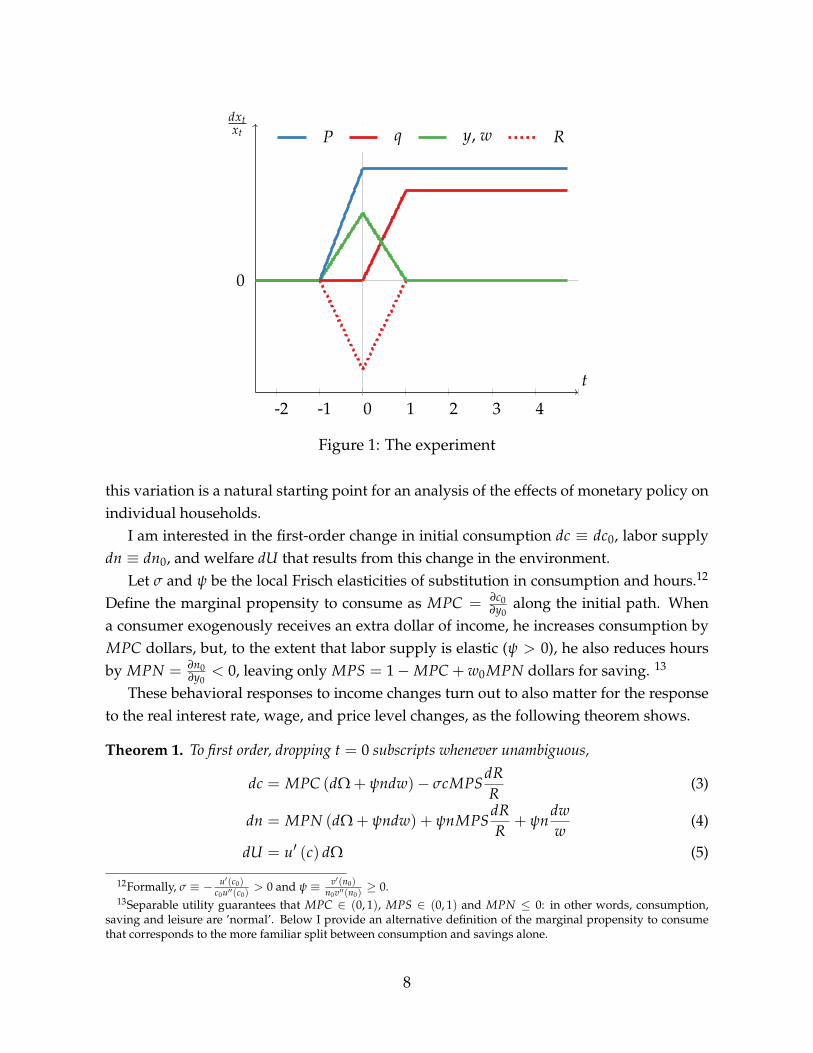
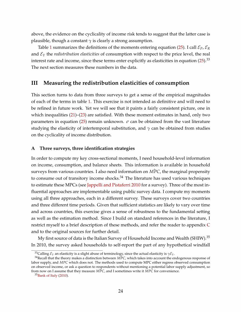
This particular variation, depicted in figure 1, captures in a stylized way the major changesin a consumer’s environment that usually follow a temporary change in monetary policy:over a period labelled t = 0, incomes and wages increase, the price level rises due toinflation between t = −1 and t = 0, and the real interest rate R0 = q0

q1falls.11 As I show

formally in appendix A.1, these are the changes that occur in the standard representative-agent New Keynesian model following a one-period change in monetary policy. Hence

11The assumption that balance sheets are fixed implies that coupon payments are not contingent on the macroe-conomic changes dw, dy, dP or dR. This is an incomplete markets assumption. If assets payoffs are state contingent,my results go through provided insurance payments are counted as part of dy.

7

-2 -1 0 1 2 3 4

0

t

dxtxt P q y, w R

Figure 1: The experiment

this variation is a natural starting point for an analysis of the effects of monetary policy onindividual households.

I am interested in the first-order change in initial consumption dc ≡ dc0, labor supplydn ≡ dn0, and welfare dU that results from this change in the environment.

Let σ and ψ be the local Frisch elasticities of substitution in consumption and hours.12

Define the marginal propensity to consume as MPC = ∂c0∂y0

along the initial path. Whena consumer exogenously receives an extra dollar of income, he increases consumption byMPC dollars, but, to the extent that labor supply is elastic (ψ > 0), he also reduces hoursby MPN = ∂n0

∂y0< 0, leaving only MPS = 1−MPC + w0MPN dollars for saving. 13

These behavioral responses to income changes turn out to also matter for the responseto the real interest rate, wage, and price level changes, as the following theorem shows.

Theorem 1. To first order, dropping t = 0 subscripts whenever unambiguous,

dc = MPC (dΩ + ψndw)− σcMPSdRR

(3)

dn = MPN (dΩ + ψndw) + ψnMPSdRR

+ ψndww

(4)

dU = u′ (c) dΩ (5)

12Formally, σ ≡ − u′(c0)c0u′′(c0)

> 0 and ψ ≡ v′(n0)n0v′′(n0)

≥ 0.13Separable utility guarantees that MPC ∈ (0, 1), MPS ∈ (0, 1) and MPN ≤ 0: in other words, consumption,

saving and leisure are ’normal’. Below I provide an alternative definition of the marginal propensity to consumethat corresponds to the more familiar split between consumption and savings alone.

8

where dΩ, the net-of-consumption wealth change, is given by

dΩ = dy + ndw−∑t≥0

Qt

(−1Bt

P0

)dPP

+

(y + wn +

(−1B0

P0

)+ (−1b0)− c

)dRR

(6)

The theorem, proved in appendix A.2, follows from an application of Slutsky’s equa-tions—separating the wealth and the substitution effects that result from the shock. Therelative price changes dR and dw generate substitution effects on consumption and la-bor supply with familiar signs, and magnitudes given by a combination of Frisch elas-ticities and marginal propensities. All wealth effects are aggregated into a net revaluationterm, dΩ, which affects consumption and labor supply after multiplication by the marginalpropensity to consume and work, respectively.

Note that theorem 1 makes no assumption on horizon or the form of u and v. In ap-pendix A.3, I show that it extends to general utility functions and to persistent shocks.

Unpacking the net wealth revaluation. The net wealth change dΩ in (6) is the keyexpression determining the sign and the magnitude of the welfare and the wealth effects intheorem 1. This term is a sum of products of balance-sheet exposures by changes in aggregates.I now describe the terms entering dΩ one by one.

The first term, dy + ndw, is the traditional effect from the change in the present value ofincome. This is the sum of the unearned income gain, dy, and the change in earned incomeholding hours fixed, ndw. When the aggregate wage increases by dw, a worker gains morewhen he initially works more hours n: we say that n represents his exposure to the wagechange. (The substitution effect on labor supply from the change in dw is not first-orderrelevant for welfare, so it does not enter dΩ.)

The second term in dΩ represents the effect from the immediate and permanent in-crease in the level of nominal prices, which matters here because of the nominal denom-ination of assets and liabilities. Define the household’s net nominal position (NNP) as thepresent value of his nominal assets, i.e.

NNP ≡ ∑t≥0

Qt

(−1Bt

P0

)We can then rewrite the second term in dΩ as −NNP dP

P , the product of exposure −NNPby inflation dP

P . Suppose for example that nominal prices unexpectedly rise by dPP = 1%.

A nominal saver with NNP = $100k experiences a wealth effect of −NNP dPP , so looses

the equivalent of $1000.14 Conversely, a nominal borrower with NNP = −$100k gains14If prices adjust more sluggishly, the Fisher exposure measure changes. For example, if prices adjust only after

T (so that dPtPt

= dPP for t ≥ T), the formulas hold if NNP is replaced by ∑t≥T Qt

(−1Bt

P0

), the present value of assets

maturing after T. In this case, short-maturity nominal assets maintain constant value, while long-maturity assetsdecline in value due to the increase in nominal discount rates that follows the expected rise in inflation. The generalexpression for any given path of price adjustment is given by formula (A.37) in appendix A.3.

9

the equivalent of $1000. These net nominal positions can be computed directly from a sur-vey of household finances. Doepke and Schneider (2006) conduct this exercise for variousgroups of U.S. households and show that NNPs are large and heterogenous in the popu-lation: they are very positive for rich, old households and negative for the young middleclass with mortgage debt. Theorem 1 shows that these numbers are not only relevant forwelfare, but also for the consumption response to this inflation scenario. Clearly, the com-position of balance sheets matters. Exposures to changes in the level of nominal pricescan be avoided by investing all wealth in inflation-indexed instruments, that is, by letting

−1Bt = 0 for all t.The final term in dΩ is the wealth effect from the change in the real interest rate. If we

define the household’s unhedged interest rate exposure, or URE, as

URE ≡ y + wn +

(−1B0

P0

)+ (−1b0)− c

then this final term is equal to URE dRR . Observe that URE is the difference between all ma-

turing assets (including income) and liabilities (including planned consumption) at time 0.It represents the net saving requirement of the household at time 0, from the point of viewof date −1. Because it includes the stocks of financial assets that mature at date 0 ratherthan interest flows, it can significantly diverge from traditional measures of savings, inparticular if investment plans have short durations.

Why is URE the correct measure of exposure following a temporary real interest ratechange dR at time 0? To fix ideas, suppose dR < 0. This is a decline in the discount rate,which results in an increase in the present value of assets (the traditional capital gainseffect). But the present value of liabilities also increases, and consumption is one suchliability. Overall, consumers experience a net wealth gain only if their future assets exceedtheir future liabilities which, in turn, can only happen if their currently-maturing liabilitiesexceed their currently-maturing assets, i.e. if URE < 0. Indeed, equation (2) implies thatthe difference between future assets and liabilities is

∑t≥1

qt (yt + wtnt) + ∑t≥1

qt

((−1bt) +

(−1Bt

Pt

))−∑

t≥1qtct = −URE

The intuition here is that a rise in the price of future consumption relative to currentconsumption (an increase in qt for t ≥ 1) is the same as a decline in the price of currentconsumption relative to future consumption (a decline in q0 holding future qt fixed). But afall in the price of current goods benefits those consumers that are demanding more goodsthan they supply at that date, and conversely, it hurts the net sellers of current goods. UREis the measure of the net exposure to this price change. As I will argue in section III, URE isalso measurable from a survey of household finances that has information on income and

10

consumption.15

This observation has the important implication that the duration of asset plans matters todetermine what happens after a change in real interest rates. Fixed rate mortgage holdersand annuitized retirees usually have income and outlays roughly balanced, and hence aURE of about zero. By contrast, ARM holders tend to have negative URE, and savers withlarge amounts of wealth invested at short durations tend to have positive URE. Hence thetheory predicts that the former tend to gain and the latter tend to loose from a temporarydecline in real interest rates.16 In response, consumption increases whenever the substitu-tion effect dominates the wealth effect. Equation 3 allows us to quantify these two effects,and shows that this happens whenever σcMPS ≥ MPC ·URE.

Monetary policy and household welfare. Theorem 1 shows that asset value changesgive incomplete information to understand the effects of monetary policy on householdwelfare. In the model just presented, monetary policy can be thought of as influencingasset values through three channels: a risk-free real discount rate effect (dR), an inflationeffect (dP), and an effect on dividends (dy). But these asset value changes do not enterdΩ directly, so they are not relevant on their own to understand who gains and who losesfrom monetary policy, contrary to what popular discussions sometimes imply. For exam-ple, it is sometimes argued that accommodative monetary policy benefits bondholders byincreasing bond prices. Yet theorem 1 shows that, while increases in dividends do raisewelfare, lower real risk-free rates have ambiguous effects on savers. They have no effecton bondholders whose dividend streams initially match the difference between their targetconsumption and other sources of income. They benefit households who hold long-termbonds to finance short-term consumption, through the capital gains they generate. Andthey hurt households who finance a long consumption stream with short-term bonds, bylowering the rates at which they reinvest their wealth. Unhedged interest rate exposures,not asset price changes, constitute the welfare-relevant metric for the impact of real interestrate changes on households. This is why it is important to measure them.

The response of consumption to overall income changes. Theorem 1 draws a dis-tinction between exogenous changes in income and changes in wages, since the latter have

15By contrast, measuring the exposure to real interest rate changes at any future date requires the knowledge offuture income and consumption plans.

16One way to understand the importance of duration is as follows. Consider an agent with financial wealthωF = $100k that is currently consuming his income c = y. Suppose first that this agent has invested all his wealthωF in one-period bonds, so that URE = ωF. Then a temporary one-year decline of 1% in the real interest raterequires him to reinvest his wealth at this lower rate, causing a net wealth loss of URE dR

R = −1000$. Supposeinstead that his wealth is entirely invested in coupon bonds maturing after the first year, so that URE = 0. In thiscase, the high interest rate on assets is ’locked in’. The net wealth effect is zero because the present value of assetsand liabilities both increase by the same amount.

11

substitution effects on consumption. However, since preferences are separable, it is possi-ble to rewrite the consumption response as a function of the total income change, inclusiveof the labor supply response, as I show in appendix A.4.

Corollary 1. Given an overall change in income dY = dy + ndw + wdn, the household’s con-sumption response is given by

dc = ˆMPC(

dY− NNPdPP

+ UREdRR

)− σc

(1− ˆMPC

) dRR

(7)

where ˆMPC = MPCMPC+MPS = MPC

1+wMPN ≥ MPC.

Hence, once we have factored in the endogenous response of income to transfers, therelevant marginal propensity to consume becomes ˆMPC, the number between 0 and 1that determines how the remaining amount of income is split between consumption andsavings. This corresponds more closely to the textbook measure of the marginal propensityto consume. It is also what empirical measures tend to pick up, since these are usuallyregressions of observed consumption on observed income.17

Durable goods. So far I have restricted my analysis to nondurable consumption. How-ever, durable expenditures tend to account for a substantial share of the overall consump-tion response to monetary policy shocks, so they are important to consider. Understandinghow durable goods fit into the theory also helps deliver an accurate map to consumptiondata. As I show formally in appendix A.5, adding durable goods to the model does notalter the substantive conclusions from Theorem 1, but there are some subtleties.

The most straightforward case is the one in which the relative price of durable goodsand nondurable goods is constant. In this case, formulas (3) or (7) continue to hold, pro-vided that c is interpreted as overall expenditures, MPC is the marginal propensity tospend on all goods, URE counts all durable expenditures as part of c, and σ is adjustedupwards to reflect the fact that durable goods allow more opportunities for intertemporalsubstitution.

In multi-sector New Keynesian models with durable goods, a constant relative priceof durable goods obtains when the prices of durables and nondurables are equally sticky(Barsky, House and Kimball 2007). However, there is some evidence that durables havemore flexible prices (e.g. Klenow and Malin 2010), in which case these models imply anegative comovement between the relative price of durables p and the nondurable realinterest rate R. Let ε = − ∂p

pR

∂R be the corresponding elasticity. When ε 6= 0, nondurables

17When hours affect the marginal utility of consumption, it is generally not possible to obtain an expression suchas (7). Instead, dw enters separately, with a sign reflecting the degree of complementarity between consumptionand labor supply.

12

and durables matter separately, so there no longer exists a straightforward notion of ag-gregate demand. Instead, in appendix A.5 I derive separate expressions for the changein nondurable and durable consumption as a function of ε. These resemble equations (3)or (7), except for the fact that the expression for c in URE only includes a share 1− ε ofdurable expenditures.18

For the purpose of measuring the size of the interest rate exposure channel, I do nothave to take a stand on the value of ε. In the empirical section, I will assume ε = 0 asa benchmark from computing UREs,19 but I will also show that my empirical results arerobust to considering alternative values for ε.

Even though all the results presented in this section assume no uncertainty and perfectforesight, they apply directly to environments with uncertainty provided that markets arecomplete, except for the shock that is unexpected (all summations are then over states aswell as dates). An important feature of all these environments is that the marginal propen-sity to consume, MPC, is the same out of all forms of wealth ( ∂c0

∂y0= ∂c0

∂ω ). The next sectionrelaxes this assumption.

C The consumption response to shocks under incomplete markets

I now consider a dynamic, incomplete-market partial equilibrium consumer choice model.Relative to the previous environment, I introduce idiosyncratic income uncertainty, restrictthe set of assets that can be traded, and consider borrowing constraints. Specifically, theconsumer now faces an idiosyncratic process for real wages wt and unearned incomeyt. He chooses consumption ct and labor supply nt to maximize the separable expectedutility function

E

[∑

tβt u (ct)− v (nt)

](8)

The horizon is still not specified in the summation: as in the previous section, it will onlyinfluence behavior through its impact on the MPC. To model market incompleteness in ageneral form, I assume that the consumer can trade in N stocks as well as in a nominallong-term bond. In period t, stocks pay real dividends dt = (d1t . . . dNt) and can be pur-chased at real prices St = (S1t . . . SNt); the consumer’s portfolio of shares is denoted by θt.Following the standard formulation in the literature, I assume that the long-term bond canbe bought at time t at price Qt and is a promise to pay a geometrically declining nominal

18When ε = 1, durable purchases are not counted at all in URE, for the same reason that purchases of bonds orshares are not: in this case, durables completely hedge real interest rate movements.

19This is a natural benchmark since an ε close to 0 is consistent with positive comovement of durables and non-durables after monetary policy shock (see Barsky, House and Kimball 2007), and would arise endogenously, forexample, if wages or intermediate goods prices are sticky, or if there are frictions to the reallocation of labor be-tween sectors in the short run.

13

coupon with pattern(1, δ, δ2, . . .

)starting at date t+ 1. The current nominal coupon, which

I denote Λt, then summarizes the entire bond portfolio, so it is not necessary to separatelykeep track of future coupons. The household’s budget constraint at date t is now

Ptct + Qt (Λt+1 − δΛt) + θt+1 · PtSt = Ptyt + Ptwtnt + Λt + θt · (PtSt + Ptdt) (9)

A borrowing constraint limits trading. This constraint specifies that real end-of-periodwealth cannot be too negative: specifically,

QtΛt+1 + θt+1 · PtSt

Pt≥ − D

Rt(10)

for some D ≥ 0, where Rt is the real interest rate at time t. The constraint in (10) is astandard specification for borrowing limits20 and we will see that it generates reactions ofconstrained agents to balance sheet revaluations that are closely related to those of uncon-strained agents. Given that the extent to which borrowing constraints react to macroeco-nomic changes is an open question, (10) provides an important benchmark.

Provided that the portfolio choice problem just described has a unique solution at datet − 1, the household’s net nominal position and his unhedged interest rate exposure areboth uniquely pinned down in each state at time t. This contrasts with the environment insection I.B, where the consumer was indifferent between all portfolio choices. Here, thesequantities are defined as

NNPt ≡ (1 + Qtδ)Λt

Pt

UREt ≡ yt + wtnt +Λt

Pt+ θt · dt − ct

As before, NNPt is the real market value of nominal wealth: the sum of the current coupon,Λt, and the value of the bond portfolio if it were sold immediately, QtδΛt. Similarly, UREt

is maturing assets (including income, real coupon payments and dividends) net of matur-ing liabilities (including consumption).

Consider the predicted effects on consumption resulting from a simultaneous unex-pected change in his current unearned income dy, his current real wage dw, the generalprice level dP and the real interest rate dR, for one period only. Assume that this variationleads asset prices to adjust to reflect the change in discounting alone : dQ

Q =dSjSj

= − dRR for

j = 1 . . . N.21 If MPC = ∂c∂y , and both MPN and MPS are similarly defined as the responses

to current income transfers, then the positive results from theorem 1 carry through.

20For example, with short-term debt and no stocks (N = δ = 0), Qt = 1Rt

PtPt+1

and (10) reads Λt+1Pt+1≥ −D , as in

Eggertsson and Krugman (2012).21This is a natural assumption that obtains if asset prices are determined in a general equilibrium with incomplete

markets. Absence of arbitrage in such a model implies the existence of a probability measure Q such that the price

of each stock j at date 0 is S0j =1

R0EQ

[∑t≥1

1R1···Rt−1

djt

], where Rt is the sequence of risk-free rates. My variation

affects R0 but does not affect future interest rates, dividends, or risk-neutral probabilities, so results in dS0jS0j

= − dRR .

14

Theorem 2. Assume that the consumer is at an interior optimum, at a binding borrowing con-straint, or unable to access financial markets (in the latter two cases, let MPS=0). Then his firstorder change in consumption dc and labor supply dn continue to be given by equations (3) and(4). In particular, writing ˆMPC ≡ MPC

MPC+MPS , the relationship between dc and the total change inincome dY = dy + ndw + wdn is still given by equation (7).

The proof is given in appendix A.6. The intuition for why MPC, MPN and MPS arerelevant to understand the response of all agents to changes in the real interest rate andthe price level is simple: when the consumer is locally optimizing, these quantities sum-marize the way in which he reacts to all balance-sheet revaluations, income being only onesuch revaluation. When the borrowing limit is binding, consumption and labor supplyadjustments depend on the way the borrowing limit changes when the shock hits. Underthe specification in (10), the changes in dR and dP free up borrowing capacity22 exactly inthe amount −NNP dP

P + URE dRR . Finally, when the consumer is unable to access financial

markets, he lives hand-to-mouth so NNP = URE = 0. In these latter two cases, ˆMPC = 1and we can interpret the consumption response as a pure wealth effect.

By showing that the marginal propensity to consume out of transitory income shocks,which has been the focus of a large empirical literature, remains a key sufficient statisticfor predicting behavior with respect to other changes in consumer balance sheets, theorem2 provides important theoretical restrictions. The rest of the paper takes these restrictionsas given and uses them to predict aggregate consumption responses to changes in R orP. But these restrictions are also directly testable empirically: given independent variationin dP, dy and dR as well as individual balance sheet information, one could check thatindividual consumption responds in accordance with equations (3) or (7). This providesan interesting avenue for future empirical work on consumption behavior.

II Aggregation and the redistribution channel

This section shows how the microeconomic demand responses derived in section I aggre-gate in general equilibrium to explain the economy-wide response to shocks in a large classof heterogenous-agent models (theorem 3).

The argument for dQ0Q0

= − dRR is identical.

22The form of the borrowing constraint in (10), which imposes a bound on the real value of wealth in period t + 1,is clearly important for this result. For example, if (10) is replaced by a constraint on the flow of income receivedfrom financial markets, QtΛt+1+θt+1·PtSt

Pt− δQtΛt+θt ·PtSt

Pt≥ −D, then the result collapses to dc = dY.

15

A Environment

Consider a closed economy populated by I heterogenous types of agents with separablepreferences (8). Each agent type i has its own discount factor βi, period utility functions ui

and vi, and time horizon. To accommodate idiosyncratic uncertainty, assume that withineach type i there is a mass 1 of individuals, each in an idiosyncratic state sit ∈ Si. I writeEI [zit] for the cross-sectional average of any variable zit, taken over individual types I andidiosyncratic states Si. I write all aggregate variables in per capita units, so for exampleaggregate (per capita) consumption Ct is equal to average individual consumption EI [cit].

Agents and asset structure. Each agent type i in state sit has a stochastic endowmentof ei (sit) efficient units of work, and receives a wage of wit = ei (sit)wt per hour, wherewt is the real wage per efficient hour. By choosing nit hours of work, he therefore receiveswteitnit in earned income. The agent also receives unearned income yit = dit − tit, the totaldividends on the trees he owns dit net of taxes from the government tit. Let the agent’soverall gross-of-tax income be

Yit ≡ wteitnit + dit. (11)

The economy has a fixed supply of aggregate capital K. A set of N trees constituteclaims to firm profits and the capital stock. Each tree delivers dividends which, in theaggregate, add up to the sum of aggregate capital income and profits: EI [dit] = ρtK + πt.Agents can also trade nominal government bonds in net supply Bt, as well as a set of J− 1additional assets in zero net supply that can be nominal or real. Each agent of type i cantrade a subset Ni of the trees and a subset Ji of the other assets. If both Ni and Ji are empty,agents of type i live hand-to-mouth. In other cases, I assume that trading is subject to atype-specific borrowing constraint Di, which takes the form in (10) and may be infinite.

Firms. There exists a competitive firm producing the unique final good in this economy,in quantity Yt and nominal price Pt, by aggregating intermediate goods with a constant-returns technology. These intermediate goods are produced by a unit mass of firms j underconstant returns to scale, using the production functions Xjt = AjtF

(Kjt, Ljt

). Markets for

inputs are perfectly competitive, so firms take the real wage wt and the real rental rate ofcapital ρt as given. These firms sell their products under monopolistic competition andtheir prices can be sticky. Firm j therefore sets its price Pjt at a markup over marginal cost,and it makes real profits πjt.23 Summing across firms j ∈ J, aggregate production is equal

23Specifically, if µjt is firm j’s markup at time t, then πjt =(

µjt − 1) (

wtLjt + ρtKjt

).

16

to aggregate income:

Yt = EJ

[Pjt

PtXjt

]= wtEJ

[Ljt]+ ρtEJ

[Kjt]+ EJ

[πjt]

(12)

Government. A government has nominal short-term debt Bt, spends Gt, and runs thetax-and-transfer system. Its nominal budget constraint is therefore:

QtBt+1 = PtGt + Bt − PtEI [tit] (13)

where Qt = 1Rt

PtPt+1

is the one-period nominal discount rate. The consequences of price-induced redistributive effects between households and the government depend cruciallyon the fiscal rule. I assume a simple rule in which the government targets a constant reallevel of debt Bt

Pt= b > 0 and spending Gt = G > 0. I also assume that the government

balances its budget at the margin by adjusting all transfers in a lump-sum manner. Hence,unexpected increases in Pt (which create ex-post deviations of Bt

Ptfrom b) and reductions in

the real interest rate Rt result in immediate lump-sum rebates.

Market clearing. In equilibrium, the markets for capital, labor and goods all clear. Thisimplies that at all times t

EJ[Kjt]≡ K (14)

EI [eitnit] = EJ[Ljt]

(15)

EI [Yit] = Yt = Ct + Gt (16)

Equilibrium also implies market clearing in all J + N asset markets. This environmentnests a large class of one-good, closed economy general equilibrium models. It can accom-modate many assumptions about population structure, asset market structure and par-ticipation, heterogeneity in preferences, endowments and skills, as well as the nature ofprice stickiness. With some minor modifications, it would accommodate wage stickinessas well. Note that the assumptions made here imply that all agents in this economy essen-tially solve either the problem in section I.A or that in section I.C.

B Aggregation result

I am interested in the aggregate consumption response to a perturbation of this environ-ment in which individual gross incomes dYi, nominal prices dP and the real interest ratedR change at t = 0 only. This exercise is useful to understand the effect of an unexpectedshock that has no persistence. Let dY ≡ EI [dYi] be the aggregate change in gross income.Assuming labor market clearing after the shock, this is also the aggregate output change.

Aggregation is simplified by several restrictions from market clearing at t = 0. Marketclearing for nominal assets implies that all nominal positions net out except for that of the

17

government,EI [NNPit] = b = −NNPgt ∀t (17)

and market clearing for all assets, combined with (11)—(16) implies24 that

EI [UREit] = Yt −EI [tit] +Bt

Pt− Ct = Gt +

Bt

Pt−EI [tit] = −UREgt (18)

where NNPgt and UREgt are naturally defined as the net nominal position and the un-hedged interest rate exposure of the government sector. Equations (17) and (18) are crucialrestrictions from general equilibrium: since one agent’s asset is another’s liability, net nom-inal positions and interest rate exposures must net out in a closed economy. Aggregationof consumer responses as described by theorem 2 shows that the per capita aggregate con-sumption change can be decomposed as the sum of five channels:

Theorem 3. To first order, in response to dYi, dY, dP and dR, aggregate consumption changes by

dC = EI

[YiY

ˆMPCi

]dY︸ ︷︷ ︸

Aggregate income channel

+CovI

(ˆMPCi, dYi −Yi

dYY

)︸ ︷︷ ︸

Earnings heterogeneity channel

−CovI( ˆMPCi, NNPi

) dPP︸ ︷︷ ︸

Fisher channel

+

CovI( ˆMPCi, UREi

)︸ ︷︷ ︸Interest rate exposure channel

−EI[σi(1− ˆMPCi

)ci]︸ ︷︷ ︸

Substitution channel

dRR

(19)

The proof is given in appendix A.7. The key step is to aggregate predictions fromtheorem 2, decomposing i’s individual income change as dYi =

YiY dY + dYi− Yi

Y dY (the sumof an aggregate component and a redistributive component), and using market clearingconditions, the fiscal rule, and the fact that EI

[dYi − Yi

Y dY]= 0 to transform expectations

of products into covariances.Theorem 3 shows that, in the class of environments I consider, a small set of sufficient

statistics is enough to understand and predict the first-order response of aggregate con-sumption to a macroeconomic shock. Equation (19) holds irrespective of the underlyingmodel generating MPCs and exposures at the micro level, as well as the relationship be-tween dY, dP and dR at the macro level. Most of the bracketed terms are cross-sectionalmoments that are measurable in household level micro-data and are informative about theeconomy’s macroeconomic response to a shock, no matter the source of this shock. The twoexceptions are the EISs σi, which need to be obtained from other sources, and dYi − Yi

dYY ,

which in general depends on the driving force behind the change in output.I now use this theorem to discuss the channels of monetary policy transmission un-

24To see this, note that if bit denotes the asset coupons that mature at time t for household i, we have UREit =Yit − tit + bit − cit. Using market clearing in the J − 1 zero net supply assets, all these coupons net out except forthe government coupon, which here is EI [bit] =

BtPt

. The result then follows from goods market clearing and thegovernment budget constraint.

18

der heterogeneity. Alternative applications, for example to short-term redistributive fiscalpolicy or open-economy models, are also possible.

C Monetary policy shocks with and without a representative agent

Consider a transitory, accommodative monetary policy shock that, as in figure 1, lowersthe real interest rate and raises aggregate income for one period (dR < 0, dY > 0), andpermanently raises the price level ( dP

P > 0). Since these are the changes implied by thetextbook New Keynesian model with sticky prices and flexible wages after a transitorymonetary policy shock, we can apply theorem 3 to understand the consumption responsein that model.

The textbook model features a representative agent (I = 1) with separable preferencesand EIS σ. Hence all covariance terms in (19) are zero, and we are left with

dC = ˆMPCdY− σ(1− ˆMPC

)C

dRR

(20)

The first term in (20) is a general-equilibrium income effect, and the second term is a sub-stitution effect.25 Solving out for dC = dY gives the textbook response, dC

C = −σ dRR .

Intuitively, a Keynesian multiplier 11− ˆMPC

amplifies the initial ’first-round’ effect from in-tertemporal substitution. Here this multiplier is entirely microfounded, and in particulartakes into account the substitution and wealth effects on labor supply that play out in thebackground.

Heterogeneity implies a role for redistributive channels in the monetary transmissionmechanism, except under special conditions. For example, if aggregate income is dis-tributed proportionally to individual income, so that dYi =

YiY dY; if no equilibrium asset

trade is possible, so that agents consume all their incomes Yi = ci and NNPi = UREi = 0;and if all agents have the same elasticity of intertemporal substitution σi = σ, then therepresentative-agent response dC

C = −σ dRR obtains even under heterogeneity. Werning

(2015) studies this important neutrality result, as well as several extensions.Away from this benchmark, the redistributive channels of monetary policy can be

signed and quantified by measuring the covariance terms in equation (19), either directlyin micro data or within a given model. In the next section, I follow the first route to obtaina sense of the plausible empirical magnitudes. As I will show, the data suggests that thefollowing is true:

CovI( ˆMPCi, UREi

)< 0 (21)

CovI( ˆMPCi, NNPi

)< 0 (22)

CovI( ˆMPCi, Yi

)< 0 (23)

25Since the typical calibration of the representative-agent model implies a low ˆMPC, the substitution componentis typically dominant in this decomposition, as noticed by Kaplan, Moll and Violante (2018).

19

These inequalities imply that redistribution amplifies the transmission mechanism of mon-etary policy.

Inequality (21) says that agents with unhedged borrowing requirements have highermarginal propensities to consume than agents with unhedged savings needs. Models withuninsured idiosyncratic risk tend to generate this as an endogenous outcome. Becauseof this interest rate exposure channel, aggregate consumption is more responsive to realinterest rates than measures of intertemporal substitution alone would suggest. In otherwords, the first-round effect of monetary policy is larger that what the representative-agentmodel predicts.

Inequality (22) says that net nominal borrowers have higher marginal propensities toconsume than net nominal asset holders. This is also an endogenous outcome of typicalincomplete market models with nominal assets. It implies that, through its general equilib-rium effect on inflation, monetary policy can increase aggregate consumption via a Fisherchannel.26

Inequality (23) says low-income agents have high MPCs, echoing a finding in much ofthe empirical literature. On its own, this fact is not enough to sign the earnings heterogene-ity channel: we need to know how increases in aggregate income affect agents at differentlevels of income. More specifically, let

γi ≡∂(

YiY − 1

)(

YiY − 1

) Y∂Y

(24)

be the elasticity of agent i’s relative income to aggregate income. Assume that this is wellapproximated by a constant γ. Then the earnings heterogeneity channel term in equation(19) simplifies to γCovI

(ˆMPCi,

YiY

)dY. There is empirical evidence that income risk is

countercyclical (for example Storesletten, Telmer and Yaron 2004 or Guvenen, Ozkan andSong 2014) and that monetary policy accommodations reduce income inequality (Coibionet al. 2017). These studies suggest that γ is negative. Combining this fact with (23), it islikely that monetary expansions increase aggregate consumption because of their endoge-nous effect on the income distribution.27

Independently of the sign of the covariance terms in (19), theorem 3 provides an or-ganizing framework for future research on the role of heterogeneity in the transmissionmechanism of monetary policy.28

26Note that this effect from redistribution is conceptually distinct from the effect of future inflation lowering realinterest rates, which has nothing to do with nominal redenomination and is present in representative-agent modelswith persistent shocks to inflation.

27Away from separable preferences, an additional complementarity channel of monetary policy can arise, even witha representative agent, when preferences are such that increases in hours worked increase the marginal utility ofconsumption.

28An early generation of papers in the heterogeneous agent New Keynesian literature analyzed the transmis-

20

D Discussion

I now provide a discussion of my result, highlighting its limitations and possible general-izations.

Interactions between the household and other sectors. The market clearing equa-tions (17) and (18) respectively state that the net nominal positions and the unhedged in-terest rate exposure of the combined household and government sectors are zero. This isa theoretical restriction that must hold in a closed economy, provided firms are correctlyconsolidated as part of the household sector. In practice there are two challenges: actualeconomies are open, and it is difficult to accurately take into account the indirect exposuresthrough firms when measuring NNPs and UREs.

In an open economy, (17) and (18) are no longer true, so price-level and real interestrate changes redistribute between the domestic economy and the rest of the world. Forexample, Doepke and Schneider (2006) find that the net nominal position of the UnitedStates is negative, implying that unexpected inflation redistributes towards the U.S. Givena positive average MPC, consumption should rise by more than what equation (19) pre-dicts. Similarly, Gourinchas and Rey (2007) find that the United States borrows short andlends long on its international portfolio, suggesting that it has a negative unhedged in-terest rate exposure. Hence, U.S. households benefit on average from lower real interestrates. This could contribute to the expansionary effects of monetary accommodations onconsumption.29

The assumption that households and firms are consolidated is also important. Forexample, the household sector tends to be maturity mismatched, holding relatively short-term assets (deposits) and relatively long-term liabilities (fixed-rate mortgages). To a largeextent, this is a counterpart to the reverse situation in the banking sector. An ideal measureof UREs and NNPs would take into account the indirect exposures that each householdhas through the firms it has a stake in. In practice, this is very challenging to do.

When we undercount household exposures to negative-URE sectors, we obtain a posi-tive EI [UREi]. This is situation also arises in the model of section II, but there the negative-URE outside sector is the government. The logic of theorem 3 shows that, if marginal re-bates from other sectors were immediate and lump-sum, this mismeasurement would be

sion of monetary policy under limited heterogeneity. In ’saver-spender’ models, such as Bilbiie (2008), ’spender’agents live hand-to-mouth and consume their incomes, so they have ˆMPC = 1; while ’saver’ agents have accessto financial markets, with a low ˆMPC. This has the effect of increasing the aggregate MPC in the economy, raisingthe importance of income effects relative to substitution effects in equation (19). In ’borrower-saver’ models, as inIacoviello (2005), the high-MPC agents are also borrowers. The literature usually assumes short-term debt, imply-ing (21) and sometimes also nominal debt, implying (22). However, whether (23) holds crucially depends on theassumptions these papers make about the distribution of wages and profits across savers vs spenders.

29To the extent that these gains are evenly distributed across the population, these effects can be quantified,respectively, by evaluating EI

[ ˆMPCi]· NNPUS and EI

[ ˆMPCi]·UREUS.

21

irrelevant. In practice, rebates are likely to be delayed, and they could disproportionatelyaffect higher or lower MPC agents, so that the numbers could depart from my benchmarkcovariance expression in either direction.

One way to assess the importance of all these effects is to directly measure in the dataexpressions such as EI

[ ˆMPCiUREi]

and to compare them to the covariance numbers.These ’no-rebate’ numbers replace the covariance terms in (19) under the assumption thatnone of the outside sectors rebate gains to the household sector. In this context, it is theoret-ically possible for the interest rate exposure term EI

[ ˆMPCiUREi]

to be both positive andlarger than the substitution term in (19). This suggests that, in a world in which outsiderebates are highly delayed or benefit low-MPC agents, real interest rate cuts could loweraggregate consumption demand, significantly altering the conventional understanding ofhow monetary policy operates.30

General equilibrium and persistent shocks. Theorem 3 provides the response ofconsumption to a transitory shock to R, P and Y. While this exercise provides an insightfuldecomposition that has the merit of involving measurable sufficient statistics, it has twomajor limitations.

First, the exercise is partial equilibrium in nature: in general, theorem 3 does not per-mit us to solve for the general equilibrium consumption effect of a given exogenous shock.This is because even transitory exogenous shocks tend to have long-lasting effects on agentbehavior and the wealth distribution, which in general equilibrium tends to generate ad-justments in future interest rates and/or income. Equation (19) does characterize the fullequilibrium in my leading case of the benchmark New Keynesian model, but in more gen-eral heterogeneous-agent models it will typically only hold as an approximation of theconsumption response to a transitory monetary policy shock.31

Second, empirically, monetary policy changes tend to be persistent. Persistent shocksmake the derivation of sufficient statistics much more difficult: for example, to characterizethe effect of future changes in R, one needs to know the distribution of future consumptionand income plans.

In the context of a given structural model, it is possible to extend my decomposition in(19) to any degree of persistence, as shown by Kaplan, Moll and Violante (2018). As modelsgrow in complexity and realism, the importance of the channels identified in Theorem 3can be assessed and refined using such a procedure. I believe that my key finding that

30This theoretical possibility is sometimes mentioned in economic discussions of monetary policy. See Raghu-ram Rajan (“Interestingly [...] low rates could even hurt overall spending”), “Money Magic”, Project Syndicate,November 11, 2013

31For instance, the theorem cannot accommodate capital investment, where a current fall in the real interest ratedR < 0 comes together with a future fall in capital income, dρ1 < 0. A previous version of this paper showed thequality of the approximation dC ' dY in the context of a model without investment.

22

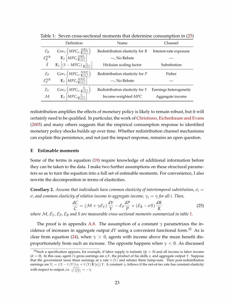
Table 1: Seven cross-sectional moments that determine consumption in (25)Definition Name Channel

ER CovI

(MPCi,

UREiEI [ci ]

)Redistribution elasticity for R Interest-rate exposure

ENRR EI

[MPCi

UREiEI [ci ]

]—, No Rebate —

S EI

[(1−MPCi)

ciEI [ci ]

]Hicksian scaling factor Substitution

EP CovI

(MPCi,

NNPiEI [ci ]

)Redistribution elasticity for P Fisher

ENRP EI

[MPCi

NNPiEI [ci ]

]—, No Rebate —

EY CovI

(MPCi,

YiEI [ci ]

)Redistribution elasticity for Y Earnings heterogeneity

M EI

[MPCi

YiEI [ci ]

]Income-weighted MPC Aggregate income

redistribution amplifies the effects of monetary policy is likely to remain robust, but it willcertainly need to be qualified. In particular, the work of Christiano, Eichenbaum and Evans(2005) and many others suggests that the empirical consumption response to identifiedmonetary policy shocks builds up over time. Whether redistribution channel mechanismscan explain this persistence, and not just the impact response, remains an open question.

E Estimable moments

Some of the terms in equation (19) require knowledge of additional information beforethey can be taken to the data. I make two further assumptions on these structural parame-ters so as to turn the equation into a full set of estimable moments. For convenience, I alsorewrite the decomposition in terms of elasticities.

Corollary 2. Assume that individuals have common elasticity of intertemporal substitution, σi =

σ, and common elasticity of relative income to aggregate income, γi = γ for all i. Then,dCC

= (M+ γEY)dYY− EP

dPP

+ (ER − σS)dRR

(25)

whereM, EY, EP, ER and S are measurable cross-sectional moments summarized in table 1.

The proof is in appendix A.8. The assumption of a constant γ parametrizes the in-cidence of increases in aggregate output dY using a convenient functional form.32 As isclear from equation (24), when γ > 0, agents with income above the mean benefit dis-proportionately from such an increase. The opposite happens when γ < 0. As discussed

32Such a specification appears, for example, if labor supply is inelastic (ψ = 0) and all income is labor income(d = 0). In this case, agent i’s gross earnings are eiY, the product of his skills ei and aggregate output Y. Supposethat the government taxes these earnings at a rate τ (Y) and rebates them lump-sum. Then post-redistributionearnings are Yi = ((1− τ (Y)) ei + τ (Y)E [ei])Y. A constant γi follows if the net-of-tax rate has constant elasticitywith respect to output, i.e. τ′(Y)

1−τ(Y) = −γ.

23

above, the evidence on the cyclicality of income risk tends to suggest that the latter case isplausible, though a constant γ is clearly a strong assumption.

Table 1 summarizes the definitions of the moments entering equation (25). I call EP, ER

and EY the redistribution elasticities of consumption with respect to the price level, the realinterest rate and income, since these terms enter explicitly as elasticities in equation (25).33

The next section measures these numbers in the data.

III Measuring the redistribution elasticities of consumption

This section turns to data from three surveys to get a sense of the empirical magnitudesof each of the terms in table 1. This exercise is not intended as definitive and will need tobe refined in future work. Yet we will see that it paints a fairly consistent picture, one inwhich inequalities (21)–(23) are satisfied. With these moment estimates in hand, only twoparameters in equation (25) remain unknown. σ can be obtained from the vast literaturestudying the elasticity of intertemporal substitution, and γ can be obtained from studieson the cyclicality of income distribution.

A Three surveys, three identification strategies

In order to compute my key cross-sectional moments, I need household-level informationon income, consumption, and balance sheets. This information is available in householdsurveys from various countries. I also need information on ˆMPC, the marginal propensityto consume out of transitory income shocks.34 The literature has used various techniquesto estimate these MPCs (see Jappelli and Pistaferri 2010 for a survey). Three of the most in-fluential approaches are implementable using public survey data. I compute my momentsusing all three approaches, each in a different survey. These surveys cover two countriesand three different time periods. Given that sufficient statistics are likely to vary over timeand across countries, this exercise gives a sense of robustness to the fundamental settingas well as the estimation method. Since I build on standard references in the literature, Irestrict myself to a brief description of these methods, and refer the reader to appendix Cand to the original sources for further detail.

My first source of data is the Italian Survey of Household Income and Wealth (SHIW).35

In 2010, the survey asked households to self-report the part of any hypothetical windfall

33Calling EY an elasticity is a slight abuse of terminology, since the actual elasticity is γEY .34Recall that the theory makes a distinction between ˆMPC, which takes into account the endogenous response of

labor supply, and MPC which does not. The methods used to compute MPC either regress observed consumptionon observed income, or ask a question to respondents without mentioning a potential labor supply adjustment, sofrom now on I assume that they measure ˆMPC, and I sometimes write it MPC for convenience.

35Bank of Italy (2010).

24

that they would immediately spend (Jappelli and Pistaferri 2014). The benefit of this ap-proach is that the windfall can be taken as exogenous for all agents, so in principle thisempirical measure of MPC is the number that matters for the theory. Another benefit ofthis survey measure is that it provides MPCs at the household level, making it easy to com-pute covariances with individual balance-sheet information. On the other hand, a concernwith self-reported answers to hypothetical situations is that they may not be informativeabout how households would actually behave in these situations. The other two measuresI consider estimate MPCs from actual behavior instead.

My second source of data is the U.S. Panel Study of Income Dynamics (PSID),36 whereI use a ’semi-structural’ approach to compute MPCs out of transitory income shocks. Theprocedure is due to Blundell, Pistaferri and Preston (2008) and has since been popularizedby Kaplan, Violante and Weidner (2014) and others. The idea is to postulate an incomeprocess and a consumption function, and to use restrictions from the theory to back outthe MPC out of transitory shocks from the joint cross-sectional distribution of consump-tion changes and income changes. Since this procedure can only recover an estimate at thegroup level, I compute my redistribution elasticities by first grouping households into dif-ferent bins, then estimating MPCs within bins and covariances across bins. One drawbackof such a procedure is that it generates large error bands.

My third source of data is the U.S. Consumer Expenditure Survey (CE),37 in whichMPC is identified using exogenous income variation following Johnson, Parker and Soule-les (2006). These authors estimate the MPC out of the 2001 tax rebate by exploiting randomvariation in the timing of the receipt of this rebate across households. Since the policy wasannounced ahead of time, they identify the MPC out of an increase in income that is ex-pected in advance. This is, in general, different from the theoretically-consistent MPC outof an unexpected increase. However, to the extent that borrowing constraints are impor-tant, or if households are surprised by the receipt despite its announcement, the resultingestimate may be close to the MPC that is important for the theory. This procedure alsoyields an MPC at a group level, so I again estimate covariances across groups, and thisalso delivers large error bands.

Each of these three techniques has its own limitations, and no survey contains perfectinformation on all components of household balance sheets. Notably, consumption in theSHIW and the PSID is imperfectly measured, as are income and assets in the CE. In ad-dition, none of these surveys samples very rich households whose consumption behaviormay be an important determinant of aggregate expenditures. Hence, the exercise in thissection is tentative and intended to give a sense of magnitudes based on the current state

36Survey Research Center, Institute for Social Research, University of Michigan (1999–2013).37U.S. Department of Labor, Bureau of Labor Statistics (2000–2002).

25

of knowledge in the field. As administrative data on consumption, income and wealthbecome available and more sophisticated identification methods for MPCs develop, a pri-ority for future work is to refine the estimates I provide here.

B Measurement

Even though my analysis is in terms of elasticities, which are unitless numbers, the choiceof temporal units is important: MPC needs to be measured over a period of time con-sistent with the time unit for income, consumption, and maturing elements of the bal-ance sheet. To maximize comparability across surveys, I conduct all my measurementat an annual rate. While this is generally straightforward to do, MPCs require specialtreatment. Specifically, in the CE, the MPC identification strategy yields a quarterly esti-mate MPCQ. I convert these to an annual MPC number MPCA using the simple formulaMPCA = 1−

(1−MPCQ)4. In appendix B, I provide a formal justification for this proce-

dure.38

MPC. I choose a benchmark of ε = 0 for the elasticity of the relative price of durables tothe real interest rate. Accordingly, my ideal measure of MPC includes total expenditureson nondurable and durable goods. The question in the SHIW refers to ’spending’ with-out distinguishing between types of purchases, so it is safe to assume that it refers to bothdurables and nondurables. For my U.S. exercises, I prefer to follow the baseline estimatesfrom Blundell, Pistaferri and Preston (2008) and Johnson, Parker and Souleles (2006), nei-ther of which include durable goods in MPC estimation. Hence, my PSID estimate onlyincludes nondurables, while my main CE estimate only includes food. In appendix C.4.1 Iconsider robustness to using total expenditures to estimate MPC instead. This makes thepoint estimates more negative, but also increases the confidence intervals. In appendixC.4.2, I consider robustness to alternative values of ε, which has a similar effect.

URE. As defined in section I.B, UREi measures the total resource flow that a householdi needs to invest over the first period of his consumption plan. In each survey, I constructUREi as

UREi = Yi − Ti − Ci + Ai − Li (26)

where Yi is gross income, Ti is taxes net of transfers, Ci is consumption, and Ai and Li

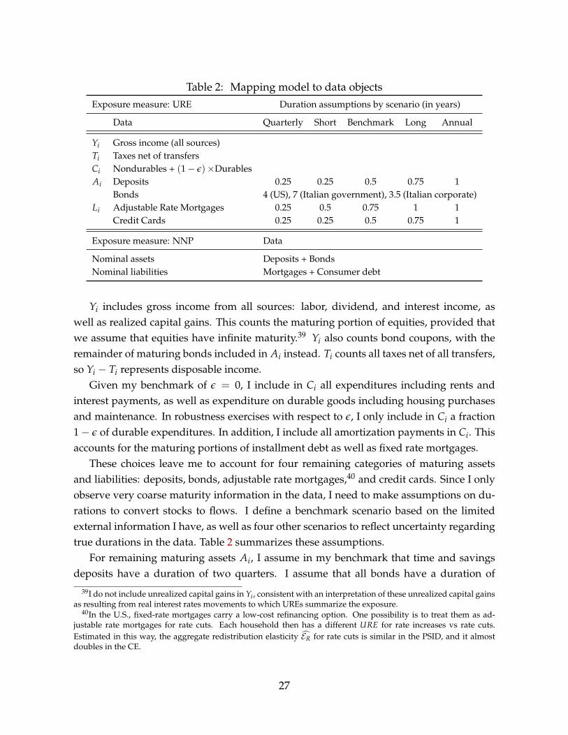
represent, respectively, assets and liabilities that mature over the period, over and abovethe amounts already included in Yi or Ci. I now describe what I include in these terms indetail. Table 2 provides a summary of the discussion that follows.

38In appendix C.4.4 I measure MPC and URE at a quarterly rate instead. This delivers similar results.

26

Table 2: Mapping model to data objectsExposure measure: URE Duration assumptions by scenario (in years)

Data Quarterly Short Benchmark Long Annual

Yi Gross income (all sources)Ti Taxes net of transfersCi Nondurables + (1− ε)×DurablesAi Deposits 0.25 0.25 0.5 0.75 1

Bonds 4 (US), 7 (Italian government), 3.5 (Italian corporate)Li Adjustable Rate Mortgages 0.25 0.5 0.75 1 1

Credit Cards 0.25 0.25 0.5 0.75 1

Exposure measure: NNP Data

Nominal assets Deposits + BondsNominal liabilities Mortgages + Consumer debt

Yi includes gross income from all sources: labor, dividend, and interest income, aswell as realized capital gains. This counts the maturing portion of equities, provided thatwe assume that equities have infinite maturity.39 Yi also counts bond coupons, with theremainder of maturing bonds included in Ai instead. Ti counts all taxes net of all transfers,so Yi − Ti represents disposable income.

Given my benchmark of ε = 0, I include in Ci all expenditures including rents andinterest payments, as well as expenditure on durable goods including housing purchasesand maintenance. In robustness exercises with respect to ε, I only include in Ci a fraction1− ε of durable expenditures. In addition, I include all amortization payments in Ci. Thisaccounts for the maturing portions of installment debt as well as fixed rate mortgages.

These choices leave me to account for four remaining categories of maturing assetsand liabilities: deposits, bonds, adjustable rate mortgages,40 and credit cards. Since I onlyobserve very coarse maturity information in the data, I need to make assumptions on du-rations to convert stocks to flows. I define a benchmark scenario based on the limitedexternal information I have, as well as four other scenarios to reflect uncertainty regardingtrue durations in the data. Table 2 summarizes these assumptions.

For remaining maturing assets Ai, I assume in my benchmark that time and savingsdeposits have a duration of two quarters. I assume that all bonds have a duration of

39I do not include unrealized capital gains in Yi, consistent with an interpretation of these unrealized capital gainsas resulting from real interest rates movements to which UREs summarize the exposure.

40In the U.S., fixed-rate mortgages carry a low-cost refinancing option. One possibility is to treat them as ad-justable rate mortgages for rate cuts. Each household then has a different URE for rate increases vs rate cuts.Estimated in this way, the aggregate redistribution elasticity ER for rate cuts is similar in the PSID, and it almostdoubles in the CE.

27

four years in the U.S., matching the average duration of assets calculated by Doepke andSchneider (2006). For Italy, where I have separate information on holdings of governmentand corporate bonds, I use the average duration of 2010 government debt documentedby the Italian Department of the Treasury (seven years), and assume that the maturity ofcorporate bonds is half as long.

For remaining maturing liabilities Li, I assume a duration of three quarters for ARMsbased on the results of Stanton and Wallace (1999). For credit cards, I assume a duration oftwo quarters. Table 2 shows my assumptions for shorter and longer duration scenarios.

NNP and income. I compute net nominal positions as the difference between directlyheld nominal assets (deposits and bonds) and directly held nominal liabilities (mortgagesand consumer credit). When assets are clearly indicated as shares of a financial interme-diary that mostly owns nominal assets (for example, money market mutual funds), I alsoinclude the value of these shares in the households’ nominal position. However, relativeto Doepke and Schneider (2006), I do not calculate the indirect nominal positions arisingfrom holdings of equity or other financial intermediaries, since my data is not sufficientlydetailed for this purpose. For my income exposure measure, in keeping with the theory, Iuse pre-tax income (Yi) in all three surveys.

Measurement error. Measurement error is a very important issue in this exercise. Theseerrors can stem from many sources: poor data quality, imperfect coverage, underreportingof consumption, or timing differences in the reporting of consumption and income. Eachsurvey has its own strengths and weaknesses. The CE has excellent information on con-sumption and liabilities, but limited information on assets. Both the PSID and the SHIWappear to significantly undermeasure consumption. My covariance estimates are unbiasedprovided that the measurement errors in in MPC and its cross-term (URE, NNP or Y) areadditive and uncorrelated. Economically, this assumption corresponds to the presence ofa ’mismeasurement’ sector that rebates gains and losses lump-sum, just as the governmentdoes in the setting of theorem 3.41 This is certainly a strong assumption. The differencebetween my benchmark elasticities and their no-rebate counterpart can give a sense of themagnitude of this mismeasurement problem.

Summary statistics. Table 3 reports the main summary statistics from each survey.Each line is normalized by average consumption in the survey, which facilitates compa-rability and corresponds to the normalization behind my elasticities in table 1. Note that

41For example, by abstracting away from indirect exposures to the banking sector, I tend to overstate the aggregateURE. If gains to the banking sector disproportionately favor low-MPC households, my estimate of the MPC/UREcorrelation would be biased downwards.

28

Table 3: Main summary statistics from the three surveysSurvey SHIW PSID CE

Variable mean s.d. mean s.d. mean s.d.

Net income (Yi − Ti) 1.19 0.83 1.42 1.64 1.14 1.01Consumption (Ci) 1.00 0.94 1.00 2.58 1.00 0.90Maturing assets (Ai) 0.93 2.48 1.30 5.06 0.53 1.77Maturing liabilities (Li) 0.31 1.40 0.51 1.44 0.52 1.47Unhedged interest rate exposure (UREi) 0.81 3.04 1.21 6.06 0.18 2.43

Nominal assets 0.74 2.36 1.18 3.66 0.47 1.84Nominal liabilities 0.50 1.49 1.73 2.75 1.22 1.90Net nominal position (NNPi) 0.24 2.64 -0.55 4.43 -0.68 2.47

Gross income (Yi) 1.27 1.04 1.69 2.51 1.23 1.09

Marginal propensity to consume (MPCi) 0.47 0.35

Number of households 7,951 7,287 4,833In each survey, ’mean’ and ’s.d.’ represent the sample mean and standard deviation.

All statistics are computed using sample weights.All variables except for MPC are normalized by average consumption in the sample.

the average URE is positive all three surveys. One reason, in addition to those highlightedin section II.D, is that consumption is below income at the mean, especially in the PSIDand the SHIW—likely because of underreporting and coverage issues. The average netnominal position is quite negative in CE and PSID—possibly reflecting a poor measureof assets—and moderately positive in the Italian survey, where few households have amortgage.

C Redistribution elasticities in the data

I now turn to my main empirical results. Figure 2 reports the distribution of MPC by URE,NNP and income across the three surveys. Columns correspond to datasets, and rowsto exposure measures. The first column displays data from the SHIW, where individualMPC information is available. The three graphs report the average value of MPC in eachpercentile of the x-axis variable. In the PSID (second column) and the CE (third column), Iestimate the MPC by stratifying the population in terciles of the x-axis variable, and thenreport the point estimate together with confidence intervals within each bin.

Starting with the interest exposure channel, looking across the first row, all three sur-veys show a negative correlation between MPC and URE. This is particularly apparent inthe SHIW and the PSID data, but the pattern is there in the CE as well. A direct implicationis that ER < 0 in each of these datasets: falls in interest rates increase consumption demand

29

-11.65 0.01 0.33 0.76 1.59 17.55

0.25

0.5

0.75

-1.22 0.48 4.37

0

0.1

0.2

-1.37 0.15 2.37

0

0.5

1

-8.53 -0.05 0.05 0.23 0.81 15.1

0.25

0.5

0.75

-3.84 -0.26 2.46

0

0.1

0.2

-3.34 -0.54 0.75

0

0.5

1

0 0.57 0.85 1.24 1.79 7.28

0.25

0.5

0.75

0.34 1.25 3.48

0

0.1

0.2

0.49 1.29 2.77

0

0.5

1

MPC

MPC

MPC

SHIW data PSID data CE data

Normalized URE Normalized URE Normalized URE

Normalized NNP Normalized NNP Normalized NNP

Normalized gross income Normalized gross income Normalized gross income

This graphs shows average annual marginal propensities to consume by exposure bin. The top row groups households by un-hedged interest rate exposure (URE), the middle row by net nominal position (NNP), and the third row by gross (pre-tax) income.The x axes report mean exposure per bin (all exposure measures are normalized by average consumption). The left column uses100 bins in the SHIW. The middle and right column uses 3 bins in the PSID and the CE, respectively, and estimate MPC withinbin. See the main text for details on MPC estimation.

Figure 2: Marginal propensities to consume and the redistribution channels.

30

Table 4: Estimates of table 1’s cross-sectional moments in three surveysSurvey SHIW PSID CE

Estimate 95% C.I. Estimate 95% C.I. Estimate 95% C.I.

ER -0.10 [–0.15,-0.05] -0.12 [-0.16,-0.08] -0.23 [-0.60,0.15]

ENRR 0.28 [0.23,0.33] 0.00 [-0.03,0.04] -0.09 [-0.48,0.31]S 0.55 [0.53,0.58] 0.90 [0.88,0.92] 0.64 [0.36,0.92]

EP -0.07 [-0.11,-0.02] 0.02 [-0.02,0.07] -0.09 [-0.51,0.33]

ENRP 0.05 [0.01,0.09] -0.01 [-0.06,0.03] -0.45 [-0.94,0.04]

EY -0.05 [-0.07, -0.03] -0.06 [-0.09,-0.04] -0.13 [-0.36,0.10]M 0.55 [0.53, 0.57] 0.08 [0.04,0.12] 0.46 [-0.06,0.98]

All statistics are computed using survey weights. In the CE and the PSID, confidence intervals are bootstrapped by resamplinghouseholds 100 times with replacement.

via the redistribution channel.Turning to the Fisher channel, we also observe an overall negative correlation in the

SHIW, though it is somewhat less pronounced. This weaker pattern is apparent in thePSID and the CE as well: in particular, MPCs tend to be slightly higher in the center ofthe NNP distribution than at the extremes. This could be consistent with a ’wealthy hand-to-mouth’ explanation as in Kaplan and Violante (2014). Overall, the slight diminishingpattern suggests that EP < 0, consistent with Fisher’s hypothesis—unexpected increasesin nominal prices tend to increase consumption overall, but this effect tends to be quanti-tatively small.

Finally, across all three surveys, the covariance between MPCs and gross incomes isalso negative, confirming previous findings in the literature. Combined with γ < 0, anegative EY implies an amplification role for the earnings heterogeneity channel in thetransmission of monetary policy.

Moving on to magnitudes, table 4 computes my seven key cross-sectional moments,together with 95% confidence intervals. For the PSID and the CE, the estimation is doneacross bins by using three bins, just as in figure 2.42

Confirming the visual impression from figure 2, the point estimates for the redistribu-tion elasticities ER, EP and EY are negative in all three surveys, except for a slight positivenumber for EP in the PSID. However, the magnitudes are relatively small—in particular,the confidence bands in the CE always include zero.43

To put these numbers in the context of standard representative-agent analyses, con-sider that many macroeconomists believe 0.1 to 0.5 as plausible values for the elasticity of

42Appendix C.4.3 reports a sensitivity analysis using four to eight bins. The results are little changed.43Moreover, the estimated value of ENR

R is usually positive, implying that the negative covariance is not strongenough to overwhelm the positive value of URE at the mean.

31

Table 5: Estimated redistribution elasticity ER for five duration scenariosDuration scenario

Quarterly Short Benchmark Long Annual

ER

SHIW-0.16 -0.20 -0.10 -0.07 -0.06

[-0.27,-0.06] [-0.27,-0.12] [-0.15,-0.05] [-0.11,-0.04] [-0.09,-0.02]

PSID-0.14 -0.13 -0.12 -0.11 -0.11

[-0.21,-0.07] [-0.20,-0.07] [-0.16,-0.08] [-0.15,-0.08] [-0.14,-0.08]

CE-0.55 -0.48 -0.23 -0.22 -0.23

[-1.35,0.24] [-1.10,0.14] [-0.60,0.15] [-0.50,0.06] [-0.49,0.03]

intertemporal substitution σ, though financial economists typically consider σ to be aboveone. (In his meta-analysis, Havránek 2015 finds a mean of σ = 0.5 but argues that it ispushed up by publication bias, while Bansal et al. 2016’s preferred estimate is σ = 2.2.)Equation (25) shows that σ should be compared to −ER/S to gauge the relative strengthof the redistribution effect. According to the point estimates from table 4, this number isbetween 0.1 and 0.4. Hence the data suggests that, if σ is as small as macroeconomiststhink, the redistribution effect may be as important as the substitution effect in explainingwhy aggregate consumption responds to changes in real interest rates. On the other hand,the magnitudes of EP and EY are fairly small, so that (unless γ is very negative) neitherchannel can account on its own for very large movements in consumption. But their com-bined effect may nevertheless be substantial, and further research is needed to refine theprecision of these estimates.

As more sources of joint consumption, income and asset data become available, a betterempirical understanding of UREs and NNPs will become possible, helping to shape ourunderstanding of the winners and losers from changes in real interest rates and inflation.Real-time estimates of the redistribution covariances could also provide useful informationabout the dynamic evolution of the monetary policy transmission mechanism.

The role of asset and liability durations. Table 5 considers the sensitivity of my esti-mates of ER to my maturity assumptions listed in table 2. In all three surveys, shorteningdurations makes the redistribution elasticity more negative, while lengthening durationsmakes it approach zero. This finding illustrates the importance of durations in determin-ing the magnitude of the interest rate exposure channel. As I discuss below, this findinghas a simple structural interpretation in incomplete market models.

32

D Empirical drivers of the redistribution covariances

While the sufficient statistic approach suggests that only the population-level redistribu-tion elasticities matter to determine an overall effect, in practice it is interesting to under-stand the empirical drivers of these covariances. For example, is the covariance betweenMPC and URE negative because older households tend to have lower MPCs and higherUREs? In order to shed light on this and related questions, I perform a covariance decom-position, projecting each covariance onto observable components such as age or education.This procedure is inspired by the law of total covariance: focusing on URE for ease of no-tation, for any covariate Zi we know that

Cov (MPCi, UREi) = Cov (E [MPCi|Zi] , E [UREi|Zi])︸ ︷︷ ︸Explained fraction of covariance

+ E [Cov (MPCi, UREi|Zi)]︸ ︷︷ ︸Unexplained fraction of covariance

(27)

We can then implement this decomposition using an OLS regression, which performs a lin-ear approximation to the conditional expectation function.44 For any observable covariateZi, I run two OLS regressions

MPCi = αM + βMZi + εMi

UREi = αR + βRZi + εRi

and compute the covariance between the fitted values MPCi and UREi to get an empiricalcounterpart of the explained component in (27). This gives me the part of the covariancethat can be explained by Zi, since

Cov (MPCi, UREi) = Cov(

MPCi + εMi, UREi + εRi

)= Cov

(βMZi + εMi, βRZi + εRi

)= Var (Zi) βM βR + Cov (εMi, εRi) (28)

where the last line follows because, by construction, Cov (εMi, Zi) = Cov (εRi, Zi) = 0. Forexample, in table 6, when Zi is age, βM is negative and βR is positive, so older agents dotend to have lower MPC and higher URE. However, on its own, age can only explain 9%of the total covariance.

This procedure is straightforward to implement in the SHIW, where MPC is availableat the individual level. Table 6 reports these results using Jappelli and Pistaferri (2014)’scontrol variables for MPC, one covariate at a time. For each of my three redistributivechannels, I report each of the terms in the decomposition (28), as well as the fraction ofthe variance explained. In appendix C.5, I generalize this approach to multiple covariates,and I also report estimates of MPC, URE and NNP by age and income bins in each survey.All of these give a consistent message: age, education and income tend to be negatively

44This is similar to implementing the law of total variance using R2.

33

Table 6: Covariance decomposition for URE, NNP and income in the SHIWER EP EY

Zi Var (Zi) βM βR % expl. βP % expl. βY % expl.Age bins 0.77 -0.027 0.467 10% 0.472 15% -0.008 -0%

Male 0.24 -0.055 0.352 5% 0.258 5% 0.271 7%Married 0.18 -0.016 0.069 0% -0.063 -0% 0.449 2%

Years of education 18.8 -0.005 0.052 5% 0.028 4% 0.097 19%Family size 1.71 0.023 -0.094 4% -0.194 12% 0.149 -11%

Resident of the South 0.22 0.198 -0.443 18% -0.231 15% -0.567 48%City size 1.21 0.037 0.013 -0% 0.048 -3% 0.058 -5%

Unemployed 0.04 0.189 -0.610 5% -0.278 3% -0.637 10%

correlated with MPC and positively correlated with URE and NNP, so they help explainthe negative covariance overall.

E Sufficient statistics: model vs data

In a previous version of this paper (Auclert 2017), I considered the sufficient statistics gen-erated by a standard partial-equilibrium incomplete markets model, similar to the oneused as a building block by the heterogeneous-agent New Keynesian literature. The modelis a Bewley-Huggett-Aiyagari model with nominal, long-term, circulating private IOUs (asin Huggett 1993). Such a model features rich heterogeneity in MPCs, UREs, NNPs and in-comes. I calibrated it to the U.S. economy and quantitatively evaluated, in its steady state,the size of my sufficient statistics. This exercise delivered three main insights.

First, in the model, the interest rate exposure channel has the same sign and compa-rable magnitude as it does in the data. Moreover, as durations shorten, the redistributionelasticity becomes more negative, consistent with my findings in table 5. In the limit whereall assets are short term, changes in real interest rates have large redistributive effects. Theintuition is as follows: the shorter asset maturities are, the less capital gains expansionarymonetary policy generates. Since capital gains accrue to low MPC agents, monetary policyis more potent in affecting consumption with short-term assets than with long-term assets.This role for asset durations is consistent with the results of Calza, Monacelli and Stracca(2013), who find that consumption reacts much more strongly to identified monetary pol-icy shocks in countries where mortgages predominantly have adjustable rates.45

Second, I find that a calibration of the model in which all assets are nominal featuresa Fisher channel with the same sign as in the data, but a much larger magnitude. Thisis because inflation redistributes along the asset dimension, which in this class of modelsis highly correlated with MPC. As a result, Bewley models with nominal assets tend to

45See also Rubio (2011) and Garriga, Kydland and Šustek (2017).

34

overstate the correlation between MPCs and NNPs that exists in the data. A model withreal assets, or in which assets have a high degree of inflation indexation, is more consistentwith the empirical evidence.

Finally, in the model with short-term debt, changes in real interest rates have asymmet-ric effects. The sufficient statistic approach correctly predicts the effect of any increase inthe real rate, but it overpredicts the effect of a large decline. This asymmetry comes fromthe differential response of borrowers at their credit limit to rises and falls in income: whilethese borrowers save an important fraction of the gains they get from low interest rates,they are forced to cut spending steeply when interest rates rise. This could help explain theempirical finding that interest rate hikes tend to lower output by more than falls increaseit (Cover 1992; de Long and Summers 1988; Tenreyro and Thwaites 2016). My explanation,which has to do with asymmetric MPC differences in response to policy rate changes, pro-vides an alternative to the traditional Keynesian interpretation of this fact, which relies ondownward nominal wage rigidities.46

IV Conclusion

This paper contributes to our understanding of the role of heterogeneity in the transmis-sion mechanism of monetary policy. I identified three important dimensions along whichmonetary policy redistributes income and wealth, and argued that each of these dimen-sions was likely to be a source of aggregate effects on consumption. My classificationholds in many environments and provides a simple, reduced-form approach to comput-ing aggregate magnitudes. Hence it can guide future work on the topic, both theoreticaland empirical.

An important finding of my paper is that capital gains and losses, both nominal andreal, matter for understanding monetary policy transmission. This finding has broad im-plications for monetary policy. A change in the inflation target can create large redistri-bution in favor of high MPC agents and be expansionary over and beyond its effect onreal interest rates. With long asset maturities, lower real interest rates can benefit assetholders with lower MPCs and make interest rate cuts less effective at increasing aggre-gate demand than they would otherwise be. Monetary policy becomes intertwined withfiscal policy, but also with government debt maturity management and mortgage designpolicies.

These are just some of the macroeconomic consequences of the presence of large andheterogeneous marginal propensities to consume, which are a robust feature of household

46In practice, the refinancing option embedded in fixed rate mortgages in the U.S. is likely to create an asymmetriceffect in the opposite direction from the one I stress here. See Wong (2018) for theory and empirical evidence alongthese lines.

35

micro data. My investigation opens up many avenues for future research on monetarypolicy with heterogeneous agents.

References

Albanesi, Stefania, “Inflation and Inequality,” Journal of Monetary Economics, May 2007, 54(4), 1088–1114.

Auclert, Adrien, “Monetary Policy and the Redistribution Channel,” Working Paper23451, National Bureau of Economic Research, May 2017.

Baker, Scott R., “Debt and the Response to Household Income Shocks: Validation andApplication of Linked Financial Account Data,” Journal of Political Economy, March 2018,126 (4), 1504–1557.

Bank of Italy, “Survey of Household Income and Wealth,” 2010.

Bansal, Ravi, Dana Kiku, and Amir Yaron, “Risks for the Long Run: Estimation with TimeAggregation,” Journal of Monetary Economics, September 2016, 82, 52–69.

Barsky, Robert B., Christopher L. House, and Miles S. Kimball, “Sticky-Price Models andDurable Goods,” American Economic Review, June 2007, 97 (3), 984–998.

Bassetto, Marco, “Optimal Fiscal Policy with Heterogeneous Agents,” Quantitative Eco-nomics, November 2014, 5 (3).

Bilbiie, Florin O., “Limited Asset Markets Participation, Monetary Policy and (inverted)Aggregate Demand Logic,” Journal of Economic Theory, May 2008, 140 (1), 162–196.

Blundell, Richard, Luigi Pistaferri, and Ian Preston, “Consumption Inequality and Par-tial Insurance,” American Economic Review, December 2008, 98 (5), 1887–1921.

Brunnermeier, Markus K. and Yuliy Sannikov, “The I Theory of Money,” Manuscript,August 2016.

Calza, Alessandro, Tommaso Monacelli, and Livio Stracca, “Housing Finance and Mon-etary Policy,” Journal of the European Economic Association, 2013, 11, 101–122.

Chetty, Raj, “Sufficient Statistics for Welfare Analysis: A Bridge Between Structural andReduced-Form Methods,” Annual Review of Economics, January 2009, 1 (1), 451–488.

Christiano, Lawrence J., Martin Eichenbaum, and Charles L. Evans, “Nominal Rigiditiesand the Dynamic Effects of a Shock to Monetary Policy,” Journal of Political Economy,February 2005, 113 (1), 1–45.

Cloyne, James, Clodomiro Ferreira, and Paolo Surico, “Monetary Policy When House-holds Have Debt: New Evidence on the Transmission Mechanism,” Review of EconomicStudies, 2018, forthcoming.

36

Coibion, Olivier, Yuriy Gorodnichenko, Lorenz Kueng, and John Silvia, “Innocent By-standers? Monetary Policy and Inequality,” Journal of Monetary Economics, June 2017, 88,70–89.

Costinot, Arnaud, Guido Lorenzoni, and Iván Werning, “A Theory of Capital Controlsas Dynamic Terms-of-Trade Manipulation,” Journal of Political Economy, February 2014,122 (1), 77–128.

Cover, James Peery, “Asymmetric Effects of Positive and Negative Money-SupplyShocks,” Quarterly Journal of Economics, November 1992, 107 (4), 1261–1282.

de Long, J. Bradford and Lawrence H. Summers, “How Does Macroeconomic Policy Af-fect Output?,” Brookings Papers on Economic Activity, January 1988, 1988 (2), 433–494.

Doepke, Matthias and Martin Schneider, “Inflation and the Redistribution of NominalWealth,” Journal of Political Economy, December 2006, 114 (6), 1069–1097.

Eggertsson, Gauti B. and Paul Krugman, “Debt, Deleveraging, and the Liquidity Trap:A Fisher-Minsky-Koo Approach,” Quarterly Journal of Economics, August 2012, 127 (3),1469–1513.

Erosa, Andrés and Gustavo Ventura, “On Inflation as a Regressive Consumption Tax,”Journal of Monetary Economics, May 2002, 49 (4), 761–795.

Fagereng, Andreas, Martib B. Holm, and Gisle J. Natvik, “MPC Heterogeneity andHousehold Balance Sheets,” Manuscript, October 2018.

Farhi, Emmanuel and Iván Werning, “Chapter 31 - Fiscal Multipliers: Liquidity Traps andCurrency Unions,” in Harald Uhlig and John B. Taylor, eds., Handbook of Macroeconomics,Vol. 2, Elsevier, 2016, pp. 2417–2492.

and , “A Theory of Macroprudential Policies in the Presence of Nominal Rigidities,”Econometrica, September 2016, 84 (5), 1645–1704.

Fisher, Irving, “The Debt-Deflation Theory of Great Depressions,” Econometrica, October1933, 1 (4), 337–357.

Galí, Jordi, J. David López-Salido, and Javier Vallés, “Understanding the Effects of Gov-ernment Spending on Consumption,” Journal of the European Economic Association, 2007,5 (1), 227–270.

Garriga, Carlos, Finn E. Kydland, and Roman Šustek, “Mortgages and Monetary Policy,”The Review of Financial Studies, October 2017, 30 (10), 3337–3375.

Gornemann, Nils, Keith Kuester, and Makoto Nakajima, “Doves for the Rich, Hawks forthe Poor? Distributional Consequences of Monetary Policy,” Manuscript, April 2016.

37

Gourinchas, Pierre-Olivier and Helene Rey, “From World Banker to World Venture Cap-italist: U.S. External Adjustment and the Exorbitant Privilege,” in “G7 Current AccountImbalances: Sustainability and Adjustment,” University of Chicago Press, 2007, pp. 11–66.

Grossman, Sanford and Laurence Weiss, “A Transactions-Based Model of the MonetaryTransmission Mechanism,” American Economic Review, December 1983, 73 (5), 871–880.

Guerrieri, Veronica and Guido Lorenzoni, “Credit Crises, Precautionary Savings, and theLiquidity Trap,” Quarterly Journal of Economics, August 2017, 132 (3), 1427–1467.

Guvenen, Fatih, Serdar Ozkan, and Jae Song, “The Nature of Countercyclical IncomeRisk,” Journal of Political Economy, June 2014, 122 (3), 621–660.

Hall, Robert E., “Intertemporal Substitution in Consumption,” Journal of Political Economy,April 1988, 96 (2), 339–357.

Harberger, Arnold C., “The Measurement of Waste,” American Economic Review Papers andProceedings, May 1964, 54 (3), 58–76.

Havránek, Tomáš, “Measuring Intertemporal Substitution: The Importance of MethodChoices and Selective Reporting,” Journal of the European Economic Association, December2015, 13 (6), 1180–1204.

Heckman, James, “Life Cycle Consumption and Labor Supply: An Explanation of the Re-lationship between Income and Consumption Over the Life Cycle,” American EconomicReview, March 1974, 64 (1), 188–194.

Huggett, Mark, “The Risk-Free Rate in Heterogeneous-Agent Incomplete-InsuranceEconomies,” Journal of Economic Dynamics and Control, September 1993, 17 (5–6), 953–969.

Iacoviello, Matteo, “House Prices, Borrowing Constraints, and Monetary Policy in theBusiness Cycle,” American Economic Review, June 2005, 95 (3), 739–764.

Jappelli, Tullio and Luigi Pistaferri, “The Consumption Response to Income Changes,”Annual Review of Economics, 2010, 2 (1), 479–506.

and , “Fiscal Policy and MPC Heterogeneity,” American Economic Journal: Macroeco-nomics, October 2014, 6 (4), 107–136.

Johnson, David S., Jonathan A. Parker, and Nicholas S. Souleles, “Household Expendi-ture and the Income Tax Rebates of 2001,” American Economic Review, December 2006, 96(5), 1589–1610.

Kaplan, Greg and Giovanni L. Violante, “A Model of the Consumption Response to FiscalStimulus Payments,” Econometrica, July 2014, 82 (4), 1199–1239.

38

, Benjamin Moll, and Giovanni L. Violante, “Monetary Policy According to HANK,”American Economic Review, March 2018, 108 (3), 697–743.

, Giovanni L. Violante, and Justin Weidner, “The Wealthy Hand-to-Mouth,” BrookingsPapers on Economic Activity, 2014, 2014 (1), 77–138.

Kimball, Miles S., “Precautionary Saving and the Marginal Propensity to Consume,”Working Paper 3403, National Bureau of Economic Research, July 1990.

King, Mervyn A., “Debt Deflation: Theory and Evidence,” European Economic Review,April 1994, 38 (3–4), 419–445.

Klenow, Peter J. and Benjamin A. Malin, “Chapter 6 - Microeconomic Evidence on Price-Setting,” in Benjamin M. Friedman and Michael Woodford, eds., Handbook of MonetaryEconomics, Vol. 3, Elsevier, 2010, pp. 231–284.

Korinek, Anton and Alp Simsek, “Liquidity Trap and Excessive Leverage,” American Eco-nomic Review, 2016, 106 (3), 699–738.

Maggio, Marco Di, Amir Kermani, Benjamin J. Keys, Tomasz Piskorski, Rodney Ram-charan, Amit Seru, and Vincent Yao, “Interest Rate Pass-Through: Mortgage Rates,Household Consumption, and Voluntary Deleveraging,” American Economic Review,November 2017, 107 (11), 3550–3588.

McKay, Alisdair and Ricardo Reis, “The Role of Automatic Stabilizers in the U.S. BusinessCycle,” Econometrica, January 2016, 84 (1), 141–194.

, Emi Nakamura, and Jón Steinsson, “The Power of Forward Guidance Revisited,”American Economic Review, October 2016, 106 (10), 3133–3158.

Mian, Atif and Amir Sufi, “What Explains the 2007–2009 Drop in Employment?,” Econo-metrica, November 2014, 82 (6), 2197–2223.

, Kamalesh Rao, and Amir Sufi, “Household Balance Sheets, Consumption, and theEconomic Slump,” Quarterly Journal of Economics, November 2013, 128 (4), 1687–1726.

Modigliani, Franco and Richard Brumberg, “Utility Analysis and the Consumption Func-tion: An Interpretation of Cross-Section Data,” in Kenneth K. Kurihara, ed., Post Keyne-sian Economics, 1954.

Oh, Hyunseung and Ricardo Reis, “Targeted Transfers and the Fiscal Response to theGreat Recession,” Journal of Monetary Economics, December 2012, 59, Supplement, S50–S64.

Rotemberg, Julio J., “A Monetary Equilibrium Model with Transactions Costs,” Journal ofPolitical Economy, February 1984, 92 (1), 40–58.

39

Rubio, Margarita, “Fixed- and Variable-Rate Mortgages, Business Cycles, and MonetaryPolicy,” Journal of Money, Credit and Banking, 2011, 43 (4), 657–688.

Sheedy, Kevin D., “Debt and Incomplete Financial Markets: A Case for Nominal GDPTargeting,” Brookings Papers on Economic Activity, 2014, pp. 301–373.

Stanton, Richard and Nancy Wallace, “Anatomy of an ARM: The Interest-Rate Risk ofAdjustable-Rate Mortgages,” The Journal of Real Estate Finance and Economics, July 1999,19 (1), 49–67.

Sterk, Vincent and Silvana Tenreyro, “The Transmission of Monetary Policy ThroughRedistributions and Durable Purchases,” Journal of Monetary Economics, November 2018,99, 124–137.

Storesletten, Kjetil, Chris I. Telmer, and Amir Yaron, “Cyclical Dynamics in IdiosyncraticLabor Market Risk,” Journal of Political Economy, June 2004, 112 (3), 695–717.

Survey Research Center, Institute for Social Research, University of Michigan, “PanelStudy of Income Dynamics, public use dataset,” 1999–2013.

Tenreyro, Silvana and Gregory Thwaites, “Pushing on a String: US Monetary Policy IsLess Powerful in Recessions,” American Economic Journal: Macroeconomics, October 2016,8 (4), 43–74.

Tobin, James, Asset Accumulation and Economic Activity: Reflections on Contemporary Macroe-conomic Theory, University Of Chicago Press, August 1982.

Tzamourani, Panagiota, “The Interest Rate Exposure of Euro Area Households,”Manuscript, April 2018.

U.S. Department of Labor, Bureau of Labor Statistics, “Consumer Expenditure Survey,Interview Survey,” 2000–2002.

Werning, Iván, “Incomplete Markets and Aggregate Demand,” Working Paper 21448, Na-tional Bureau of Economic Research, August 2015.

Wong, Arlene, “Transmission of Monetary Policy to Consumption and Population Aging,”Manuscript, January 2018.

40

Monetary Policy and the Redistribution Channel

Online Appendix

Adrien Auclert†

A Proofs for sections I and II

A.1 The standard New Keynesian model

This section shows that, in the standard New Keynesian model with sticky Calvo prices, the impulseresponse to the path for prices Pt, real discount rates qt, real wages wt and unearned income are thosegiven by my main experiment in figure 1. I only outline the elements of the model relevant to myargument, the reader is referred to the textbook treatments of Woodford (2003) or Galí (2008) for details.

I consider the model in its ’cashless limit’, with no aggregate uncertainty. The model features arepresentative agent with separable utility trading in one-period nominal bonds and holding a fixedstock of capital k, so equation (1) simplifies to

∑ βt u (ct)− v (nt)

Ptct + (tQt+1) Bt+1 = Ptπt + Wtnt + Bt + Ptρtk

Here ρt denotes the real rental rate of capital, so ρtk are total real rents, and πt are real firm profits. To-gether, rents and profits make up the unearned income in this economy. Consumption ct is an aggregateof intermediate goods, with constant elasticity of substitution ε. Hence the price index, aggregating the

individual goods prices pjt, is Pt =(∫ 1

0 p1−εjt dj

) 11−ε .

Each good j is produced under monopolistic competition with constant returns to scale and unitproductivity. The production function is

yjt = F(k jt, ljt

)= kα

jtl1−αjt

Firms can only adjust their price with probability θ each period, independent across firms and periods(the Calvo assumption). Nominal wages Wt and nominal rents are flexible. Cost minimization by thefirm therefore implies

ρtPt = ΛjtFk(k jt, ljt

)Wt = ΛjtFl

(k jt, ljt

)for some scalar Λjt representing the nominal marginal cost of production for firm j. Hence

Fk(k jt, ljt

)Fl(k jt, ljt

) =Fk

( kjtljt

, 1)

Fl

( kjtljt

, 1) =

ρt

wt

† Last update: September 2019. I thank Thomas Hintermaier for carefully reading through the proof and point-ing out typos in the derivation of Theorem 1. (These do not affect the final result as stated in the paper.)

A1

so all firms have the same capital-labor ratiokjtljt

= ktlt

, and hence all firms have the same nominalmarginal cost of production Λt.

As is well-known, a first-order approximation to the equilibrium equations of this model is given bythe system of three equations

log( ct

c

)= log

( ct+1

c

)− σ

(it − log

(Pt+1

Pt

)− $

)(A.1)

log(

Pt

Pt−1

)= β log

(Pt+1

Pt

)+ κ log

( ct

c

)(A.2)

it = $ + φπ log(

Pt

Pt−1

)+ εt (A.3)

where c is the level of consumption that would prevail under flexible prices, which (normalizing k = 1)solves

v′((c)

11−α

)u′ (c)

=ε− 1

ε

(1− α)

c≡ w

$ = β−1 − 1 is the steady-state net real interest rate, σ = − u′(c)cu′′(c)

is the elasticity of substitution around

c, and κ is the slope of the Phillips curve (a function of model parameters). Equation (A.3) is a Taylorrule describing the behavior of monetary policy. We assume that φπ > 1, which guarantees equilibriumuniqueness. We consider the effects of a time-0 monetary policy loosening, ε0 < 0 and εt = 0 for t ≥ 1,assuming the system was at steady-state at t = −1, with constant price level P.

It is easy to guess and verify that the equilibrium features it = ρ, Pt = Pt−1 and ct = c for t ≥ 1.Solving backwards, this implies that

i0 = ρ +1

1 + κσφπε0

log( c0

c

)= − σ

1 + κσφπε0

log(

P0

P

)= − κσ

1 + κσφπε0

In other words, a monetary loosening raises ct at t = 0 only, and raises Pt immediately and permanently.(Firms that get an opportunity to reset at t = 0 all increase their price above P, pulling up the price levelto P0. Thereafter, all firms that get a chance reset their price to P0, so there is no inflation.) To a first-orderapproximation, the real wage satisfies

wt =

v′(

c1

1−αt

)u′ (ct)

so wt increases at t = 0 only and then reverts to w. Moreover, real rents are

ρt =α

1− αwtc

11−αt

so they also increase at t = 0 and then revert to ρ = α1−α w (c)

11−α . 47 Date-0 nominal and real state prices

47Since price dispersion rises as a result of the monetary policy shock, the nonlinear solution features a real wagethat is different from steady state even beyond t ≥ 1, but the difference is second order in ε0.

A2

are Q0 = q0 = 1 and, for t ≥ 1, given that Pt = P0,

qt = Qt =t−1

∏s=0

(sQt) =1

1 + i0βt−1

Hence, the path of qt and Qt for t ≥ 1 is shifted upwards by dqtqt

= dQtQt

= − dRR where the proportional

real interest rate change is dRR = dε0

(1+κσφπ)1

(1+ρ). Finally, aggregate profits are, to first-order, given by

πt = ct − wtnt − ρtk = ct

1− 11− α

v′((ct)

11−α

)u′ (ct)

ct

(A.4)

Hence they also deviate only at t = 0 from their steady state value of d = cε . The first term in (A.4) is

volume, which rises with c0. The second term is the markup, which falls with c0. In typical calibrations,the markup effect dominates and profits fall in response to an expansionary monetary shock ε0 < 0.

Collecting results, the timing of changes for wt, Pt and qt, as well as unearned income ρtk + πt, isexactly that depicted in figure 1, as claimed in the main text.

A.2 Proof of theorem 1

The proof is greatly simplified by first applying a simple renormalization of discount factors. Instead ofthe present value normalization q0 = 1, I normalize q1 = 1 and let q0 vary. Then, setting

dq0

q0=

dRR

(A.5)

yields the experiment in figure 1. Intuitively, a rise in the relative price of future goods relative to acurrent good is the same as a fall in the price of that current good relative to all future goods. Thisrenormalization is innocuous since there is a degree of freedom in choosing discount factors.

Given the experiment, we can hold qt fixed for t ≥ 1. Hence, only three parameters y0, w0 and q0vary, together with the sequence Pt.

With this renormalization, the proof has three steps: first, I apply Slutsky’s theorem to break downdc and dn into income and substitution effects. Second, I work out explicit expressions for MPC andMPN. Finally, I calculate compensated derivatives, and use my expressions from the second step tosimplify their expressions.

Step 1: Slutsky’s theorem. Recall that the sequences qt and wt are fixed in the experiment,except for q0 and w0. Define the following expenditure function

e (q0, w0, U) = min

∑

tqt (ct − wtnt) s.t. ∑

tβt u (ct)− v (nt) ≥ U

(A.6)

A3

and let ch0, nh

0 be the resulting compensated (Hicksian) demands for time-0 consumption and hours.Applying the envelope theorem, we obtain a version of Shephard’s lemma:

eq0 = c0 − w0n0 (A.7)

ew0 = −q0n0 (A.8)

Define ’unearned’ wealth as

ω ≡ ∑t≥0

qt

(yt + (−1bt) +

(−1Bt

Pt

))and note that, given the variation we consider,

dω =

(y0 + (−1b0) +

(−1B0

P0

))dq0 + q0dy0 −∑

t≥0qt

(−1Bt

Pt

)dPt

Pt(A.9)

Using the Fisher equation qtPt

= QtP0

, and the fact that dPtPt

= dPP is a constant, the last term rewrites

∑t≥0

qt

(−1Bt

Pt

)dPt

Pt= ∑

t≥0Qt

(−1Bt

P0

)dPP

= q0NNPdPP

where we have defined the household’s net nominal position as the present value of his nominal assets

q0NNP ≡ ∑t≥0

Qt

(−1Bt

P0

)

Moreover, defining

URE ≡ w0n0 + y0 + (−1b0) +

(−1B0

P0

)− c0

we can rewrite (A.9) as

dω = (URE + c0 − w0n0) dq0 + q0dy0 − q0NNPdPP

(A.10)

Next, define the indirect utility function that attains ω as

V (q0, w0, ω) = max

∑

tβt u (ct)− v (nt) s.t. ∑

tqt (ct − wtnt) = ω

(A.11)

Let c0, n0 denote the resulting Marshallian demands. Applying the envelope theorem, we find

∂V∂q0

= −u′ (c0)

q0(c0 − w0n0) (A.12)

∂V∂w0

=u′ (c0)

q0q0n0 (A.13)

∂V∂ω

=u′ (c0)

q0(A.14)

A4

As in the proof of Slutsky’s theorem, we next differentiate along the identities

ch0 (q0, w0, U) = c0 (q0, w0, e (q0, w0, U))

nh0 (q0, w0, U) = n0 (q0, w0, e (q0, w0, U))

to find that Marshallian and Hicksian derivatives are related via

∂ch0

∂q0=

∂c0

∂q0+

∂c0

∂ωeq0

∂ch0

∂w0=

∂c0

∂w0+

∂c0

∂ωew0 (A.15)

∂nh0

∂q0=

∂n0

∂q0+

∂n0

∂ωeq0

∂nh0

∂w0=

∂n0

∂w0+

∂n0

∂ωew0 (A.16)

Next, define

MPC ≡ q0∂c0

∂ω(A.17)

MPN ≡ q0∂n0

∂ω(A.18)

these express the dollar-for-dollar (or hour-for-dollar) marginal propensities to consume and work atdate 0: indeed,

∂c0

∂y0=

∂c0

∂ω

∂ω

∂y0=

MPCq0

q0 = MPC

and similarly ∂n0∂y0

= MPN.Totally differentiating the Marshallian consumption function and using (A.10), we find

dc0 =∂c0

∂q0dq0 +

∂c0

∂w0dw0 +

∂c0

∂ω

((URE + c0 − w0n0) dq0 + q0dy0 − q0NNP

dPP

)Using (A.15)–(A.16),

dc0 =

(∂ch

0∂q0− ∂c0

∂ωeq0

)dq0 +

(∂ch

0∂w0− ∂c0

∂ωew0

)dw0

+∂c0

∂ω

((URE + c0 − w0n0) dq0 + q0dy0 − q0NNP

dPP

)=

∂c0

∂ω

(−ew0 dw0 + q0dy0 +

(−eq0 + URE + c0 − w0n0

)dq0 − NNP

dPP

)+

∂ch0

∂q0dq0 +

∂ch0

∂w0dw0

and using (A.7), (A.8) and (A.17) to replace ew0 , eq0 and ∂c0∂ω , we find

dc0 =MPC

q0

(q0n0dw0 + q0dy0 + UREdq0 − q0NNP

dPP

)+

∂ch0

∂q0dq0 +

∂ch0

∂w0dw0

= MPC(

n0dw0 + dy0 + UREdq0

q0− NNP

dPP

)+ c0

(q0

c0

∂ch0

∂q0

dq0

q0+

w0

c0

∂ch0

∂w0

dw0

w0

)

Finally, dropping time subscripts for ease of notation, using (A.5), and defining compensated elasticities

A5

by

εhc,q ≡ q0

c0

∂ch0

∂q0

εhc,w ≡ w0

c0

∂ch0

∂w0

we obtain

dc = MPC(

ndw + dy + UREdRR− NNP

dPP

)+ c

(εh

c,qdRR

+ εhc,w

dww

)(A.19)

In a completely analogous way, we also find

dn = MPN(

ndw + dy + UREdRR− NNP

dPP

)+ n

(εh

n,qdRR

+ εhn,w

dww

)(A.20)

The rest of the proof calculates the compensated elasticities and relates them to MPC and MPN,which will yield our expressions for consumption and labor supply. To get my expression for welfare,totally differentiate the indirect utility function and use (A.12)–(A.14) and (A.10) to obtain

dU =∂V∂q0

dq0 +∂V∂w0

dw0 +∂V∂ω

dω

=u′ (c0)

q0·(

UREdq0 + q0n0dw0 + q0dy0 − q0NNPdPP

)This yields my expression in (5),

dU = u′ (c) ·(

dy + ndw + UREdRR− NNP

dPP

)

Step 2: Marginal propensities. I now derive explicit expressions for marginal propensities to con-sume, that is, the Marshallian derivatives of the consumption and labor supply functions that are solu-tions to (A.11). Inverting the first-order conditions

u′ (ct) = β−t(

qt

q0

)u′ (c0) (A.21)

v′ (nt) = β−t(

qt

q0

)(wt

w0

)v′ (n0) (A.22)

and inserting the resulting values for ct and nt into the budget constraint (redefining W = ωq0

as present-value wealth for simplicity)

∑t≥0

qt

q0(ct − wtnt) = W

we obtain

c0 + ∑t≥1

qt

q0

(u′)−1

[β−t

(qt

q0

)u′ (c0)

]− w0

(n0 + ∑

t≥1

qt

q0

wt

w0

(v′)−1

[β−t

(qt

q0

)(wt

w0

)v′ (n0)

])= W

(A.23)

A6

Recall that MPC = ∂c0∂W and MPN = ∂n0

∂W . Differentiating (A.23) with respect to W, we obtain

MPC

(1 + ∑

t≥1

qt

q0β−t

(qt

q0

)u′′ (c0)

u′′ (ct)

)− w0MPN

(1 + ∑

t≥1

qt

q0

wt

w0β−t

(qt

q0

)(wt

w0

)v′′ (n0)

v′′ (nt)

)= 1 (A.24)

moreover, the intratemporal first order condition

v′ (n0) = w0u′ (c0) (A.25)

implies

v′′ (n0) MPN = w0u′′ (c0) MPCv′′ (n0)

v′ (n0)MPN =

u′′ (c0)

u′ (c0)MPC

so, using the definition of the local elasticities of substitution,

−σ (ct) ctu′′ (ct) = u′ (ct) (A.26)

ψ (nt) ntv′′ (nt) = v′ (nt) (A.27)

we see that MPC and MPN are related through

MPN = −ψ (n0)

σ (c0)

n0

c0MPC

Inserting into (A.24), this gives

MPC =

(1 + ∑

t≥1

qt

q0β−t

(qt

q0

)u′′ (c0)

u′′ (ct)+

ψ (n0)

σ (c0)

w0n0

c0

(1 + ∑

t≥1

qt

q0

wt

w0β−t

(qt

q0

)(wt

w0

)v′′ (n0)

v′′ (nt)

))−1

(A.28)as well as

MPS = 1−MPC + w0MPN

= MPC

(∑t≥1

qt

q0β−t

(qt

q0

)u′′ (c0)

u′′ (ct)

+ψ (n0)

σ (c0)

w0n0

c0∑t≥1

qt

q0

wt

w0β−t

(qt

q0

)(wt

w0

)v′′ (n0)

v′′ (nt)

)(A.29)

Expressions (A.28) and (A.29) can also be rewritten using the fact that (A.21)-(A.22) together with (A.26)-(A.27) yield

β−t(

qt

q0

)u′′ (c0)

u′′ (ct)=

σ (ct) ct

σ (c0) c0β−t

(qt

q0

)(wt

w0

)v′′ (n0)

v′′ (nt)=

ψ (nt) nt

ψ (n0) n0

A7

So, we also have

MPC =

(1 + ∑

t≥1

qt

q0

σ (ct) ct

σ (c0) c0+

ψ (n0)

σ (c0)

w0n0

c0

(1 + ∑

t≥1

(qt

q0

)(wt

w0

)ψ (nt) nt

ψ (n0) n0

))−1

Step 3: Hicksian elasticities. The solution to the expenditure minimization problem in (A.6) alsoinvolves the first-order conditions (A.21)-(A.22) , from which we obtain

u (ct) = u((

u′)−1

[β−t

(qt

q0

)u′ (c0)

])v (nt) = v

((v′)−1

[β−t

(qt

q0

)(wt

w0

)v′ (n0)

])attaining utility U requires that the initial values c0, n0 satisfy

u (c0) + ∑t≥1

βtu((

u′)−1

[β−t

(qt

q0

)u′ (c0)

])− v (n0)

−∑t≥1

βtv((

v′)−1

[β−t

(qt

q0

)(wt

w0

)v′ (n0)

])= U (A.30)

Differentiating with respect to q0 along the indifference curve (A.30) results in

∂c0

∂q0

(u′ (c0) + ∑

t≥1βtu′ (ct) β−t

(qt

q0

)u′′ (c0)

u′′ (ct)

)

−∂n0

∂q0

(v′ (n0) + ∑

t≥1βtv′ (nt) β−t

(qt

q0

)(wt

w0

)v′′ (n0)

v′′ (nt)

)

−∑t≥1

βt u′ (ct)

u′′ (ct)

(β−t qt

q20

u′ (c0)

)−∑

t≥1βt v′ (nt)

v′′ (nt)

(β−t qt

q20

(wt

w0

)v′ (n0)

)= 0

dividing by u′ (c0) and using (A.21), (A.25), (A.26) and (A.27) we find

∂c0

∂q0

(1 + ∑

t

qt

q0β−t

(qt

q0

)u′′ (c0)

u′′ (ct)

)− ∂n0

∂q0w0

(1 + ∑

t≥1

qt

q0

wt

w0β−t

(qt

q0

)(wt

w0

)v′′ (n0)

v′′ (nt)

)

=1

u′ (c0)

(∑t≥1

βt u′ (ct)

u′′ (ct)

(β−t qt

q20

u′ (c0)

)+ ∑

t≥1βt v′ (nt)

v′′ (nt)

(β−t qt

q20

(wt

w0

)v′ (n0)

))

moreover, differentiating (A.25) we also find

∂n0

∂q0= −ψ (n0)

σ (c0)

n0

c0

∂c0

∂q0

A8

Gathering results, we recognize, on the left-hand-side, the MPC expression in (A.28). We then use first-order conditions on the right hand side to obtain

∂c0

∂q0MPC−1 =

1u′ (c0)

∑t≥1

βt u′ (ct)

u′′ (ct)

(β−t qt

q20

u′ (c0)

)−∑

t≥1βt v′ (nt)

v′′ (nt)

(β−t qt

q20

(wt

w0

)v′ (n0)

)

=1q0

(∑t≥1

u′ (ct)

u′′ (ct)

qt

q0− w0 ∑

t≥1

v′ (nt)

v′′ (nt)

qt

q0

(wt

w0

))

Manipulating the right-hand side, we recognize the expression for (A.29) as

∂c0

∂q0MPC−1 = − 1

q0σ (c0) c0

∑t≥1

β−t(

qt

q0

)u′′ (c0)

u′′ (ct)

qt

q0

+w0n0

c0

ψ (n0)

σ (c0)∑t≥1

β−t(

qt

q0

)(wt

w0

)v′′ (n0)

v′′ (nt)

qt

q0

(wt

w0

)

= − 1q0

σ (c0) c0MPSMPC

and therefore, we finally simply have

∂c0

∂q0

⌋U

= − c0

q0σ (c0) MPS

which corresponds to a Hicksian elasticity of

εhc0,q0

= −σ (c0) MPS (A.31)

A similar procedure can be used to differentiate with respect to w0: from (A.25) we obtain

∂n0

∂w0= −ψ (n0)

σ (c0)

n0

c0

∂c0

∂w0+ ψ (n0)

n0

w0

and differentiating along (A.30) we therefore obtain

∂c0

∂w0u′ (c0) MPC−1 − ψ (n0)

n0

w0

(v′ (n0) + ∑

t≥1βtv′ (nt) β−t

(qt

q0

)(wt

w0

)v′′ (n0)

v′′ (nt)

)

= ∑t≥1

βt v′ (nt)

v′′ (nt)β−t qt

q0

(wt

w20

)v′ (n0)

We conclude by noticing that v′ (n0) = ψ (n0) n0v′′ (n0), so

∂c0

∂w0

⌋U= MPCψ (n0) n0

and

εhc0,w0

= MPC(

ψ (n0)w0n0

c0

)(A.32)

A9

Finally, elasticities for n0 result from a final differentiation of (A.25):

εhn0,q0

= −ψ (n0)

σ (c0)εh

c0,q0(A.33)

εhn0,w0

= ψ (n0)

(1− 1

σ (c0)εh

c0,w0

)= ψ (n0)

(1− ψ (n0)

σ (c0)

w0n0

c0MPC

)= ψ (n0) (1 + w0MPN) (A.34)

Step 4: Putting all expressions together. For consumption, equations (A.31)–(A.32) can be insertedinto (A.19) to yield

dc = MPC(

ndw + dy + UREdRR− NNP

dPP

)+ c

(−σMPS

dRR

+ ψMPCwnc

dww

)The first term is the wealth effect, and the last two terms the substitution effects with respect to interestrates and wages. We then simplify the expression to

dc = MPC(

dy + n (1 + ψ) dw + UREdRR− NNP

dPP

)− σcMPS

dRR

(A.35)

which is our equation (3).Similarly, equations (A.33)–(A.34) can be inserted into (A.20) to yield

dn = MPN(

ndw + dy + UREdRR− NNP

dPP

)+ n

(ψMPS

dRR

+ ψ (1 + wMPN)dww

)and we again naturally separate the latter piece to obtain

dn = MPN(

dy + n (1 + ψ) dw + UREdRR− NNP

dPP

)+ ψnMPS

dRR

+ ψndww

(A.36)

which is equation (4).

A.3 Extension of Theorem 1 to general preferences and persistent changes

Theorem 1 in the main text is a special case of a general decomposition that holds for arbitrary nonsa-tiable preferences U over ct and nt and for any change in the price level P0, P1 . . ., the real termstructure q0 = 1, q1, q2 . . ., the agent’s unearned income sequence y0, y1 . . . and the stream of realwages w0, w1 . . ., with the nominal term structure adjusting instantaneously to make the Fisher equa-tion hold at the post-shock sequences of interest rates and prices. The utility maximization problem isthen

max U (ct, nt)s.t. Ptct = Ptyt + Wtnt + (t−1Bt) + ∑

s≥1(tQt+s) (t−1Bt+s − tBt+s)

+Pt (t−1bt) + ∑s≥1

(tqt+s) Pt+s (t−1bt+s − tbt+s)

A10

and the first order date-0 responses of consumption, labor supply and welfare to the considered changeare, in this case, given by

dc0 = MPCdΩ + c0

(∑t≥0

εhc0,qt

dqt

qt+ ∑

t≥0εh

c0,wt

dwt

wt

)

dn0 = MPNdΩ + n0

(∑t≥0

εhn0,qt

dqt

qt+ ∑

t≥0εh

n0,wt

dwt

wt

)dU = Uc0 dΩ

where εhx0,yt =

∂xh0

∂yt

ytx0

for x ∈ c, n and y ∈ q, w are Hicksian elasticities and dΩ = dW − ∑t≥0 ctdqt,the net-of-consumption wealth change, is given by

dΩ = ∑t≥0

(qtyt)dyt

yt︸ ︷︷ ︸Real unearned income change

+ ∑t≥0

(qtwtnt)dwt

wt︸ ︷︷ ︸Real earned income change

+ ∑t≥0

qt

(yt + wtnt +

(−1Bt

Pt

)+ (−1bt)− ct

)dqt

qt︸ ︷︷ ︸Revaluation of net savings flows

− ∑t≥0

Qt

(−1Bt

P0

)dPt

Pt︸ ︷︷ ︸Revaluation of net nominal position

(A.37)

The proof is a generalization of that in section A.2. I omit it here in the interest of space.

Values of all elasticities with separable preferences in a steady-state with no growth. Fol-lowing once more the steps of section A.2, it is possible to derive the value of Hicksian elasticities for achange at any horizon. Here I just report the values of these elasticities in the case of an infinite horizonmodel where qs

q0= βs and ws = w∗, ∀s. These prices correspond to those prevailing in a steady-state with

no growth of any such model, and the resulting elasticities are relevant, for example, to determine theimpulse responses in many RBC and DSGE models. The first order conditions imply that consumptionand labor supply are constant. Let us call the solutions c∗ and n∗, respectively. Writing ϑ ≡ w∗n∗

c∗ for the

share of earned income in consumption and κ ≡ψσ ϑ

1+ ψσ ϑ∈ (0, 1), obtain values of elasticities summarized

in table A.1.

Table A.1: Steady-state moments, separable preferencesεh q0 qs,s ≥ 1 w0 ws,s ≥ 1 Marg. propensityc0 −σβ σ (1− β) βs σκ (1− β) σκ (1− β) βs MPC (1− κ) (1− β)n0 ψβ −ψ (1− β) βs ψ (1− κ (1− β)) −ψκ (1− β) βs MPN − 1

w∗ κ (1− β)MPS (1− β)

A11

A.4 Proof of corollary 1

Rewrite equations (A.35) and (A.36) as

dc = MPC(

dY + ψdw− wdn + UREdRR− NNP

dPP

)− σcMPS

dRR

wdn− ψndw = wMPN(

dY + ψdw− wdn + UREdRR− NNP

dPP

)+ ψwnMPS

dRR

Hence

wdn− ψndw =1

1 + wMPN

wMPN

(dY + URE

dRR− NNP

dPP

)+ ψwnMPS

dRR

which, inserted into the expression for dc yields

dc = MPC(

1− wMPN1 + wMPN

)(dY + URE

dRR− NNP

dPP

)−σcMPS

(1 + MPC

ψwnσc

11 + wMPN

)dRR

But MPC ψnσc = −MPN so this is

dc =(

MPC1 + wMPN

)(dY + URE

dRR− NNP

dPP

)− σc

MPS1 + wMPN

dRR

and noting that1 + wMPN = MPC + MPS

we can finally rewrite this in terms of ˆMPC = MPCMPC+MPS as

dc = ˆMPC(

dY + UREdRR− NNP

dPP

)− σc

(1− ˆMPC

) dRR

as claimed.

A.5 Adding durable goods

This section shows the consequences of adding durable goods to the model.I consider a standard durable goods problem. For simplicity, I ignore labor supply and nominal

assets, neither of which interacts with the conclusions below. A consumer maximizes a separable in-tertemporal utility function

max ∑ βt u (Ct) + w (Dt)s.t. Ct + pt It = Yt + (t−1bt) + ∑

s≥1(tqt+s) (t−1bt+s − tbt+s)

Dt = It + Dt−1 (1− δ)

D−1, −1bt given

where Ct is now nondurable consumption, Dt is the consumer’s stock of durables, and pt is the relativeprice of durable goods in period t.

A12

I am interested in the response of the demand for nondurable goods Ct and durables goods It, aswell as that of total expenditures

Xt ≡ Ct + pt It (A.38)

to a change in the time-0 nondurable real interest rate R0 and (potentially) a simultaneous change inthe price of durables p0. As I argue below, the notion of aggregate demand makes most sense when therelative price of durables does not change with R0, but I start by covering the general case in which p0can change.

The intertemporal budget constraint reads

∑t≥0

qt (Ct + pt It) = ∑t≥0

qtYt + ∑t≥0

qt (−1bt)

Defining Rt ≡ qtqt+1

, the first-order conditions of this problem are, for all t ≥ 0

u′ (Ct) = βRtu′ (Ct+1) (A.39)

w′ (Dt) = u′ (Ct)

[pt −

(1− δ) pt+1

Rt

](A.40)

Equation (A.39) is the standard Euler equation for nondurable consumption. Equation (A.40) shows thatthe consumer equates the marginal rate of substitution between the stock of durables and consumptionto the user cost of durables, pt − (1−δ)pt+1

Rt. A fall in the nondurable real interest rate at date 0, R0,

increases the desired level of nondurable consumption and of the stock of nondurables (an intertemporalsubstitution effect). Holding p1 constant, it also reduces the user cost of durables, increasing the desiredstock of durables relative to nondurable consumption. A fall in p0 has the same effect of reducing thedurable user cost, but it does not affect intertemporal substitution in consumption.

Suppose that the path for interest rates Rt, relative prices pt and income Yt delivers the so-lution Ct, Dt. Consider the solution under the alternative paths

R0, R1, R2 . . .

, p0, p1, p2 . . ., and

Y0, Y1, Y2 . . .

. Let dR = R0 − R0, dp = p0 − p0 and dY = Y0 − Y0. I am interested in the response ofthe paths of nondurable and durable expenditures to these changes. To obtain this, I find the paths forconsumption Ct and durables Dt, and then find the implied path for durable expenditures pt It.

Marshallian demand. In order to determine the Marshallian demands, I could follow the sameproof as that of section A.2, but here I follow an alternative and somewhat more intuitive procedure.The procedure is in two steps. First, I determine a variation that respects all the first-order conditions(A.39)–(A.40) at the new prices. This gives dC∗ and dD∗, which result in a budgetary cost dΩ∗ at theold prices. Second, I determine the change in net wealth dΩ that results from the change in prices. TheMarshaling demands are then

dC = dC∗ + MPC (dΩ− dΩ∗) (A.41)

dD = dD∗ + MPD (dΩ− dΩ∗) (A.42)

where MPD = ∂D∂Y is the increase in the stock of date-0 durables that results from a date-0 increase in

income. Note that MPC and MPD are related: differentiating (A.40), we find

w′′ (D0) MPD = u′′ (C0) MPC[

p0 −(1− δ) p1

R0

]

A13

soMPD =

σDσC

D0

C0MPC

where σC ≡ − u′(C0)u′′(C0)C0

and σD ≡ − w′(D0)w′′(D0)D0

are the elasticities of intertemporal substitution in con-sumption and in the stock of durables. Since D0 = I0 + D−1 (1− δ) and the initial stock D−1 is fixed,the total constant-p marginal propensity to spend at date 0 is

MPX ≡ ∂ (C + pI)∂Y

=∂C∂Y

+ p∂D∂Y

= MPC + pMPD

= MPC(

1 +σDσC

pDC

)

Step 1: variation respecting FOCs. The simplest variation that respects all FOCs holds the pathsCt and Dt fixed for all t ≥ 1 and adjusts C0 and D0 by dC (respectively dD) such that (A.39) and(A.40) are satisfied at t = 0. Differentiating these equations, I obtain

− 1σC

dCC

=dRR

− 1σD

dDD

= − 1σC

dCC

+p1

1−δR

p0 − p11−δ

R

dRR

+p0

p0 − p11−δ

R

dpp

Hence we finddC∗ = −σCC

dRR

(A.43)

and

dD∗ = −σDD

[p0

p0 − p11−δ

R

](dRR

+dpp

)(A.44)

These responses are very intuitive: one way to respond to a fall in real interest rates is to raise nondurableconsumption and the stock of durables. The relevant elasticity for durables is higher than σD becauseof the additional substitution effect coming from the change in the user cost. A lower current relativeprice of durables has a symmetric effect on the demand for durables as that of a lower real interest rate(in other words, it is the real interest rate in terms of durables that matters for durables demand).

We are now ready to determine the net cost of this variation. Since

D0 = (1− δ) D−1 + I0

D1 = (1− δ) D0 + I1

the sequence of investment that achieves this variation consists naturally in an increase of dD∗ followedby a subsequent decrease:

dI∗0 = dD∗

dI∗1 = − (1− δ) dD∗

A14

Hence the total budgetary cost of this ’star’ variation at the old prices p and R has the simple form

dΩ∗ = dC∗ + p0dI∗0 + p1dI∗1R

= dC∗ +(

p0 − p11− δ

R

)dD∗

= − (σCC + p0σDD)dRR− σD p0D

dpp

Step 2: change in net wealth. Let Ω be defined as

Ω ≡ ∑t≥0

qt Yt + (−1bt)− Ct − pt It .

At the initial prices, the intertemporal budget constraint implies Ω = 0. The exogenous variation dR, dpand dY yields

dΩ = dY− Idp + ∑t≥0

dqt Yt + (−1bt)− Ct − pt It

= dY− Idp−∑t≥1

qt Yt + (−1bt)− Ct − pt ItdRR

= dY− pI0dpp

+

Y0 + (−1b0)− C0 − p0 I0︸ ︷︷ ︸URE

dRR

(A.45)

The intuition is as follows. Suppose that the nondurable real interest rate falls at date 0. As before, thisbenefits consumers that have a negative URE, that is, maturing liabilities C0 + p0 I0 in excess maturingassets Y0 + (−1b0). Note that, for this effect, total expenditures including expenditures on durables arecounted as part of URE. In that sense, URE measures the true balance-sheet exposure to a change in thereal interest rate. In particular, ceteris paribus, when investment is higher today the consumer benefitsmore from a fall in real interest rates.

Suppose however that, in parallel, the relative price of durables rises. In the general equilibriummodel of Barsky, House and Kimball (2007), for example, this happens in response to an accommodativemonetary policy shock when durable goods prices are more flexible than nondurable goods prices. Inthat case, equation (A.45) shows that there is an additional capital loss on wealth due to the rise in thedurable relative price. While conceptually distinct, these two effects could be consolidated into a singleone, if we restrict ourselves to variations that feature a constant elasticity of the durable-good price tothe nondurable real interest rate

εpR ≡ −∂pp

R∂R

(A.46)

The benchmark case where p is constant corresponds to εpR = 0, the case where the durable real interestrate is constant to εpR = 1. Then,

dΩ = dY +

Y0 + (−1b0)− C0 − p0 I0(1− εpR

)︸ ︷︷ ︸UREε

dRR

(A.47)

A15

In other words, once we net out the capital revaluation effect, an alternative measure of URE becomesUREε, which subtracts a fraction

(1− εpR

)of durable expenditures.

Step 3: demand for durables and nondurables. Combining (A.41)–(A.42) with (A.43), (A.44)and (A.45), I obtain the Marshallian demands (recall that dI = dD at time 0)

dC = MPC(

dY + UREdRR

+ (σCC + pσDD)dRR

+ (pσDD− pI0)dpp

)− σCC

dRR

dD = MPD(

dY + UREdRR

+ (σCC + pσDD)dRR

+ (pσDD− pI0)dpp

)−σDD

[p0

p0 − p11−δ

R

](dRR

+dpp

)

This separates out the separate effects from changing R and p. Given the elasticity εpR in (A.46), we canalso rewrite this as

dC = MPC(

dY + UREε dRR

)− σCC (1−MPC)

dRR

+σD · pD ·MPC ·(1− εpR

)· dR

R(A.48)

dD = MPD(

dY + UREε dRR

)+ σC ·MPD · C · dR

R

−σD · pD ·(1− εpR

)· (1−MPD) ·

[1

p0 − p11−δ

R

]dRR

(A.49)

Where UREε is defined in (A.47).

Special case with constant durable real interest rate (εpR = 1). When εpR = 1, equations(A.48)–(A.49) simplify to

dC = MPC(

dY + URE1 dRR

)− σCC (1−MPC)

dRR

dD = MPD(

dY + URE1 dRR

)+ σC ·MPD · C · dR

R

which are simple extensions of expressions in the main text, with URE1 (which does not subtract durableexpenditures) replacing URE. Note that to the extent that URE1 ≥ 0, the expression for dD implies acontraction in durable goods from an increase in real interest rates, as in Barsky, House and Kimball(2007). This is counterfactual, suggesting that εpR = 1 may be too high an elasticity in practice.

Special case with constant relative price (εpR = 0). While the cases where εpR 6= 0 are interestingin principle, they prevent a straightforward definition of aggregate demand X = C + pI: if the relativeprice of two goods can change, then the relative demands for these two goods (as well as their relativesupplies) will matter for general equilibrium. Therefore, the case where εpR = 0 is the most relevantfor my purposes. Assume then that p0 = p1 = p. In this case, we can combine (A.48) and (A.49) toobtain an expression for the change in aggregate demand dX = dC + pdD as a function of the marginal

A16

propensity to spend MPX = MPC + pMPD and other variables

dX = MPX(

dY + UREdRR

+ σCC + σD pD)−(

σCC +σD pD

1− 1−δR

)dRR

This can further be simplified to yield an expression with the same form as the expression in the maintext,

dX = MPX(

dY + UREdRR

)− σX (1−MPX) X

dRR

(A.50)

where σX is defined as

σX ≡CX· σC +

(1− C

X

)· σD ·

pDpI·

11− 1−δ

R−MPX

1−MPX(A.51)

In other words, σX is a weighted average of σC and the relevant elasticity of substitution in durableexpenditures: the product of σD by the stock-flow ratio pD

pI , multiplied by a term that increases in theelasticity of the user cost to the real interest rate.

Quantitatively, the second term is likely to be much larger than the first. If initially durable expendi-tures cover replacement costs I = Dδ, then the stock-flow ratio is 1

δ . Hence, with δ = 5% and R = 1.05 atannual rates, the second term in (A.51) is at least as large as 1

20 × 110 × σD = 200σD. This makes aggregate

demand very sensitive to given changes in the real interest rate because of the large substitution effectthat results from the presence of long-lived durables, a point made by Barsky et al. (2007).

A.6 Proof of theorem 2

After dividing through by Pt, defining the real bond position as λt ≡ ΛtPt−1

and writing Πt ≡ PtPt−1

for theinflation rate between t− 1 and t, the budget constraint (9) becomes

ct + Qt

(λt+1 − δ

λt

Πt

)+ (θt+1 − θt) · St = yt + wtnt +

λt

Πt+ θt · dt

In this notation, the consumer’s date-t net nominal position is

NNPt = (1 + Qtδ)λt

Πt

while his unhedged interest rate exposure is:

UREt = yt + wtnt +λt

Πt+ θt · dt − ct = Qt

(λt+1 − δ

λt

Πt

)+ (θt+1 − θt) · St

A17

His optimization problem can be represented using the recursive formulation

maxc,n,λ′ ,θ′

u (c)− v (n) + βE[V(λ′, θ′; y′, w′, Q′, Π′, d′, S′

)]︸ ︷︷ ︸≡W(λ′ ,θ′)

s.t. c + Q(

λ′ − δλ

Π

)+(θ′ − θ

)S = y + wn +

λ

Π+ θd (A.52)

Qλ′ + θ′S ≥ DR

The function V corresponds to the value from optimizing given a starting real level of bonds λ′ andshares θ′, and includes the possibility of hitting future borrowing constraints.

I consider the predicted effects on c and n resulting from a simultaneous unexpected change inunearned income dy, the real wage dw, the price level dP

P = dΠΠ and the real interest rate dR, which

result in a change in asset prices dQQ =

dSjSj

= − dRR for j = 1 . . . N. By leaving the future unaffected, this

purely transitory change does not alter the value from future optimization starting at (λ′, θ′)— that is,the function W is unchanged. I claim that, provided the consumption and labor supply functions aredifferentiable, their first order differentials are

dc = MPC(

dy + n (1 + ψ) dw + UREdRR− NNP

dPP

)− σcMPS

dRR

(A.53)

dn = MPN(

dy + n (1 + ψ) dw + UREdRR− NNP

dPP

)+ ψnMPS

dRR

+ ψndww

(A.54)

where σ ≡ − u′(c)cu′′(c) and ψ = v′(n)

nv′′(n) are the local elasticities of intertemporal substitution and labor

supply, respectively, MPC = ∂c∂y , MPN = ∂n

∂y and MPS = 1−MPC + wMPN.In order to prove (A.53) and (A.54), there are two cases to consider. In the first case, the consumer is

at a binding borrowing limit or lives hand-to-mouth. The problem is then a static choice between c andn. In the second case, the consumer is at an interior optimum. The result then follows from application ofthe implicit function theorem to the set of N + 2 first-order conditions which, together with the budgetconstraint, characterize the solution to the problem in (A.52). Here, to simplify the notation and theproof, I first prove the statement in the case where all variables are changing but N = 0, and thenconsider the case with stocks (N > 0) but without bonds and assuming only R is changing.

Case 1. Binding borrowing limit and hand-to-mouth agents.

Proof. The consumption of an agent at the borrowing limit is given by

c = wn + Z (A.55)

where

Z = z + (1 + Qδ)λ

Π+ θ · (d + S) +

DR

Similarly, the consumption of an agent that lives hand to mouth is

c = wn + z

Given that dS = − SR dR, dQ = −Q

R dR and d(

1Π

)= − 1

Π2 dΠ = − 1Π

dPP , we have, if the agent is at the

A18

borrowing limit

dZ = dz− (1 + Qδ)λ

Π︸ ︷︷ ︸NNP

dPP

+

(Qδ

λ

Π+ θ · S +

DR

)︸ ︷︷ ︸

−URE

(−dR

R

)(A.56)

and, if the agent lives hand to mouth,dZ = dz

but since that agent also hasNNP = URE = 0

equation (A.56) still applies. In both cases, the consumer is making a static choice between c and n giventhe budget constraint (A.55), and hence has MPS = 0. We can then apply the results of section A.2 tofind

dc = MPC (dZ + w (1 + ψ))

dn = MPN (dZ + w (1 + ψ)) + ψndw

which yields the desired result.

Case 2a). N = 0, all variables changing I first prove the following lemma.

Lemma A.1. Let c (z, w, q, b) and n (z, w, q, b) be the solution to the following separable consumer choice problemunder concave preferences over current consumption u (c) and assets V (a), and convex preferences over hoursworked v (n):

max u (c)− v (n) + V (a)

s.t. c + q (a− b) = wn + z

Assume c () and n () are differentiable. Then the first order differentials are

dc = MPC (dz + n (1 + ψ) dw− (a− b) dq + qdb)− σcMPSdqq

dn = MPN (dz + n (1 + ψ) dw− (a− b) dq + qdb) + ψnMPSdqq

+ ψndww

where MPC = ∂c∂z , MPN = ∂n

∂z and MPS = 1−MPC + wMPN = 1−MPC(

1 + wnc

ψσ

).

Proof. The following first-order conditions are necessary and sufficient for optimality:

u′ (c) =1w

v′ (n) =1q

V′ (a) (A.57)

I first obtain the expression for MPC by considering an increase in income dz alone. Consider how thatincrease is divided between current consumption, leisure and assets. (A.57) implies

u′′ (c) dc =1w

v′′ (n) dn =1q

V′′ (a) da (A.58)

A19

where the changes dc, dn and da are related to dz through the budget constraint

dc + qda = wdn + dz (A.59)

Define MPC = ∂c∂z , MPN = ∂n

∂z and MPS = q ∂a∂z . Then (A.58) implies

MPNMPC

= wu′′ (c)v′′ (n)

=u′′ (c)u′ (c)

v′ (n)v′′ (n)

= −nc

ψ

σ

MPSMPC

=q2u′′ (c)V′′ (a)

=qc

V′ (a)σV′′ (a)

where σ ≡ − u′(c)cu′′(c) and ψ ≡ v′(n)

nv′′(n) . Hence the total marginal propensity to spend is

1−MPS =∂c∂z− w

∂n∂z

= MPC(

1 +wnc

ψ (n)σ (c)

)= 1− q2u′′ (c)

V′′ (a)MPC (A.60)

and the marginal propensity to consume is

MPC =1

1 + q2 u′′(c)V′′(a) − w2 u′′(c)

v′′(n)

=V′′ (a) v′′ (n)

V′′ (a) v′′ (n) + q2u′′ (c) v′′ (n)− w2u′′ (c)V′′ (a)

Consider now the overall effect on c, n and a of a change in q, w, z and b. Applying the implicit functiontheorem to the system of equations

v′ (n)− wu′ (c) = 0

V′ (a)− qu′ (c) = 0

c + q (a− b)− wn− z = 0

results in the following expression for partial derivatives:

∂c∂q

∂c∂z

∂c∂w

∂c∂b

∂n∂q

∂n∂z

∂n∂w

∂n∂b

∂a∂q

∂a∂z

∂a∂w

∂a∂b

= −

−wu′′ (c) v′′ (n) 0−qu′′ (c) 0 V′′ (a)

1 −w q

−1

︸ ︷︷ ︸≡A

0 0 −u′ (c) 0−u′ (c) 0 0 0(a− b) −1 −n −q

(A.61)

now

det (A) = v′′ (n)V′′ (a)− w2u′′ (c)V′′ (a) + q2u′′ (c) v′′ (n) =V′′ (a) v′′ (n)

MPC

and so

A−1 =MPC

V′′ (a) v′′ (n)

wV′′ (a) −v′′ (n) q v′′ (n)V′′ (a)q2u′′ (c) + V′′ (a) −wqu′′ (c) wu′′ (c)V′′ (a)

qwu′′ (c) w2u′′ (c)− v′′ (n) qu′′ (c) v′′ (n)

A20

therefore, the first row of (A.61)

[∂c∂q

∂c∂z

∂c∂w

∂c∂b

]= MPC

[− w

v′′(n)q

V′′(a) −1] 0 0 −u′ (c) 0−u′ (c) 0 0 0(a− b) −1 −n −q

(A.62)

Using (A.60) we find

−qu′ (c)

V′′ (a)MPC =

σcq

q2 u′′ (c)V′′ (a)

MPC =σcq

MPS

so that the first column of the matrix equation (A.62) reads

∂c∂q

=σcq

MPS− (a− b) MPC

The second and fourth column of (A.62) yield directly

∂c∂z

= MPC

∂c∂b

= qMPC

Finally, using (A.57) we have

wu′ (c)v′′ (n)

=v′ (n)v′′ (n)

= ψn

so that the third column of (A.62) reads

∂c∂w

= MPCψn + MPCn

= MPC (1 + ψ) n

The first-order total differential dc is then

dc =∂c∂z

dz +∂c∂b

db +∂c∂q

dq +∂c∂w

dw

= MPC (dz + qdb− (a− b) dq + (1 + ψ) ndw) + σcMPSdqq

(A.63)

as claimed. Similarly, after using MPN = MPCw u′′(c)v′′(n) , the second row of (A.61) is

[∂n∂q

∂n∂z

∂n∂w

∂n∂b

]= MPN

[− q2+V′′(a)/u′′(c)

wV′′(a)q

V′′(a) −1] 0 0 −u′ (c) 0−u′ (c) 0 0 0(a− b) −1 −n −q

(A.64)

Using (A.60) we find

−qu′ (c)

V′′ (a)MPN =

σcq

q2 u′′ (c)V′′ (a)

MPC(−nψ

σc

)= −nψ

qMPS

A21

Again the first column yields∂c∂q

= −nψ

qMPS− (a− b) MPN

The second and fourth column of (A.62) yield directly

∂c∂z

= MPN

∂c∂b

= qMPN

Finally, since (q2 +

V′′ (a)u′′ (c)

)u′ (c)

V′′ (a)= −σc

(q2 u′′ (c)

V′′ (a)+ 1)

= ψnMPCMPN

(MPSMPC

+ 1)

the third column yields

∂n∂w

=1w

ψn (MPS + MPC) + MPNn =1w

ψn (1 + wMPN) + MPNn = ψn1w

+ MPN (n + ψn)

The first-order total differential dn is then

dn =∂n∂z

dz +∂n∂b

db +∂n∂q

dq +∂n∂w

dw

= MPN (dz + qdb− (a− b) dq + (1 + ψ) ndw)− ψnMPSdqq

+ ψndww

(A.65)

Proof of theorem 2 in case 2a). If the policy functions are differentiable and the consumer is at an interioroptimum, then the conditions of lemma A.1 are satisfied: the borrowing constraint is not binding socan be ignored, and the value function is concave per standard dynamic programming arguments. Thenotation of theorem 2 can be cast using that of the lemma by using the mapping

q ≡ Q z ≡ y +λ

Πa ≡ λ′ b ≡ δ

λ

Π

with dPP = dΠ

Π and dQQ = − dR

R . Hence dz = dy− λΠ

dPP , db = −δ λ

ΠdPP and dq

q = − dRR ; so

dz + qdb− (a− b) dq = dy− (1 + Qδ)λ

Π︸ ︷︷ ︸NNP

dPP

+

(λ′ − δ

λ

Π

)Q︸ ︷︷ ︸

URE

dRR

Inserting this equation into (A.63) and (A.65) yields the desired result.

Case 2b) N > 0, no bonds, only R changing. Since we are not considering changes in wages, itis sufficient to restrict the analysis to a choice between consumption and assets. The following lemma

A22

then proves the result for dc. The result for dn follows as a straightforward extension.

Lemma A.2. Let c (θ, Y, R) be the solution to the following consumer choice problem under concave preferencesover current consumption u (c) and assets W (θ′)

maxc,θ′ u (c) + W(θ′)

s.t. c +(θ′ − θ

)S = Y + θd

where dSdR = − S

R . Then, to first order

dc = MPC(

dY + UREdRR

)− σ (c) c (1−MPC)

dRR

where σ (c) ≡ − u′(c)cu′′(c) is the local elasticity of intertemporal substitution, MPC = ∂c

∂Y , and URE = Y + θd− c

Proof. The following first-order conditions characterize the solution

Siu′(Y + θd−

(θ′ − θ

)S)= Wθi

(θ′)∀i = 1 . . . N (A.66)

Consider first an increase in income dY alone. Differentiating along (A.66) we find

Siu′′ (c)

(1−∑

jSj dθ

′ j

dY

)= ∑

jWθiθ j

(θ′) dθ

′ j

dY∀i (A.67)

Define η j ≡ Sj dθ′ j

dY . Then (A.67) rewrites

∑j

(1

SiSj Wθiθ j(θ′)+ u′′ (c)

)η j = u′′ (c) ∀i

Defining the matrix M with elements

mij ≡1

SiSj Wθiθ j(θ′)+ u′′ (c)

this system can also be written in matrix form as

Mη = u′′ (c) 1

orη = u′′ (c) M−11

The budget constraint then implies that

MPC =dcdY

= 1−∑j

η j = 1− u′′ (c)m (A.68)

where m is defined asm ≡ 1M−11 (A.69)

A23

Next, consider an increase in the real interest rate dR. Differentiating along (A.66) we now have

dSi

dRu′ (c) + Siu′′ (c)

(−∑

jSj dθ

′ j

dR−∑

j

dSj

dR

(θ′ j − θ j

))= ∑

jWθiθ j

(θ′) dθ

′ j

dR∀i

Using dSi

Si = − dRR this rewrites

−Si

Ru′ (c) + Siu′′ (c)

(−∑

jSj dθ

′ j

dR+ ∑

j

Sj

R

(θ′ j − θ j

))= ∑

jWθiθ j

(θ′) dθ

′ j

dR∀i (A.70)

Defining now γj ≡ Sj dθ j′

dR , (A.70) shows that γj solves

∑j

mijγj = − 1

Ru′ (c) + u′′ (c)∑

j

Sj

R

(θ′ j − θ j

)∀i

which rewrites in matrix form

Mγ =

(− 1

Ru′ (c) + u′′ (c)∑

j

Sj

R

(θ′ j − θ j

))1

or

γ =

(− 1

Ru′ (c) + u′′ (c)∑

j

Sj

R

(θ′ j − θ j

))M−11 (A.71)

Differentiating with respect to R along the budget constraint c = Y + θd− (θ′ − θ) S, we next see that

dcdR

= −∑j

Sj θ′ j

dR+ ∑

j

Sj

R

(θ j − θ

′ j)= −∑

jγj + ∑

j

Sj

R

(θ j − θ

′ j)

inserting (A.71) and using the definition of m,

dcdR

= −(− 1

Ru′ (c) + u′′ (c)∑

j

Sj

R

(θ′ j − θ j

))m + ∑

j

Sj

R

(θ j − θ

′ j)

(A.72)

rearranging terms and using u′ (c) ≡ −cσ (c) u′′ (c) we find

dcdR

= −σ (c)cR

u′′ (c)m + ∑j

Sj

R

(θ′ j − θ j

) (1− u′′ (c)m

)But using the expression for MPC in (A.68), this is simply

dcdR

= −σ (c)cR(1−MPC) + ∑

j

Sj

R

(θ j′ − θ j

)MPC

A24

and using the budget constraint ∑j Sj(

θ j′ − θ j)= (θ′ − θ) · St = URE we obtain

dcdR

= −σ (c)cR(1−MPC) +

1R

URE ·MPC (A.73)

Finally, considering a simultaneous change in income and the real interest rate, combining (A.68) and(A.73) we obtain the first order differential

dc = MPC(

dY + UREdRR

)− σ (c) c (1−MPC)

dRR

as was to be shown.

A.7 Proof of theorem 3

Given the assumption of fixed balance sheets and purely transitory shocks, Theorem 2 shows that

dci = ˆMPCi

(dYi − dti + UREi

dRR− NNPi

dPP

)− σici

(1− ˆMPCi

) dRR

where, where dYi = nieidw + weidni + d (di) is the change in gross income at the individual level anddti the change in taxes. We can further decompose the change in gross income as

dYi =YiY

dY + dYi −YiY

dY

and note that, since EI [Yi] = Y,

EI

[dYi −

YiY

dY]= dY− EI [Yi]

YdY = 0 (A.74)

Hence,

dci = ˆMPCi

(YiY

dY + dYi −YiY

dY− dti + UREidRR− NNPi

dPP

)− σici

(1− ˆMPCi

) dRR

and taking a cross-sectional average

dC = EI

[YiY

ˆMPCi

]dY + EI

[ˆMPCi

(dYi −

YiY

dY)]−EI

[ ˆMPCi (dti)]−EI

[ ˆMPCi NNPi] dP

P

+(EI[ ˆMPCiUREi

]−EI

[σi(1− ˆMPCi

)ci]) dR

R(A.75)

Now, the government budget (13) with the fiscal rule Gt = G and target BtPt

= b reads

EI [tit] = G +Bt

Pt− b

Rt

A25

Using the fact that at the margin, taxes are adjusted lump-sum, and the fact that NNPg = −b as well as

UREg = − bR , this implies

dti = dt = NNPgdPP−UREg

dRR

In other words, taxes fall with unexpected increases in prices which reduce the government debt burden,and they fall with reductions in real interest rates which reduces the government’s debt servicing costs.But the market clearing conditions (17) and (18) imply that these gains and losses have counterparts atthe household level:

dti = dt = −EI [NNPi]dPP

+ EI [UREi]dRR

(A.76)

Hence, (A.75) rewrites

dC = EI

[YiY

ˆMPCi

]dY + EI

[ˆMPCi

(dYi −

YiY

dY)]−EI

[ ˆMPCi](dt)−EI

[ ˆMPCi NNPi] dP

P

+(EI[ ˆMPCiUREi

]−EI

[σi(1− ˆMPCi

)ci]) dR

R

so

dC = EI

[YiY

ˆMPCi

]dY + EI

[ˆMPCi

(dYi −

YiY

dY)]

+ EI[ ˆMPCi

]EI [NNPi]

dPP−EI

[ ˆMPCi NNPi] dP

P

+(EI[ ˆMPCiUREi

]−EI

[ ˆMPCi]

EI [UREi]−EI[σi(1− ˆMPCi

)ci]) dR

R

and finally, using (A.74)

dC = EI

[YiY

ˆMPCi

]dY + CovI

(ˆMPCi, dYi −Yi

dYY

)−CovI

( ˆMPCi, NNPi) dP

P

+(CovI

( ˆMPCi, UREi)−EI

[σi(1− ˆMPCi

)ci]) dR

R

as claimed.

Case with heterogeneous taxes. If the taxes were not lump-sum, equation (A.76) would be replacedby

EI [dti] = −EI [NNPi]dPP

+ EI [UREi]dRR

we would therefore use the fact that

EI[ ˆMPCi (dti)

]= EI

[ ˆMPCi]

EI [dti] + CovI( ˆMPCi, dti

)to finally obtain

dC = EI

[YiY

ˆMPCi

]dY + CovI

(ˆMPCi, dYi −Yi

dYY

)−CovI

( ˆMPCi, NNPi) dP

P

+(CovI

( ˆMPCi, UREi)−EI

[σi(1− ˆMPCi

)ci]) dR

R−CovI

( ˆMPCi, dti)

The additional heterogeneous-taxation term is very natural. Suppose for example that, at the margin,gains from the government budget (EI [dti] < 0) lead to disproportionate reductions of taxes on high-

A26

MPC agents. Then CovI( ˆMPCi, dti

)< 0 , so aggregate consumption increases by more than the bench-

mark from Theorem 1. The opposite happens when tax reductions fall disproportionately on low-MPCagents.

A.8 Proof of corollary 2

From the definition of γi in (24), we have

d(

YiY

)= γi

(YiY− 1)

dYY

Moreover,

dYi −YidYY

= Yd(

YiY

)= γi

(YiY− 1)

dY (A.77)

Next, rewrite equation (19) in elasticity terms by dividing by per-capita consumption C = EI [ci] andusing (A.77). We find

dCC

= EI

[Yi

EI [ci]ˆMPCi

]dYY︸ ︷︷ ︸

Aggregate income channel

+CovI

(ˆMPCi, γi

YiEI [ci]

)︸ ︷︷ ︸Earnings heterogeneity channel

dYY −CovI

(ˆMPCi,

NNPiEI [ci]

)dPP︸ ︷︷ ︸

Fisher channel

+

CovI

(ˆMPCi,

UREiEI [ci]

)︸ ︷︷ ︸Interest rate exposure channel

−EI

[σi(1− ˆMPCi

) ciEI [ci]

]︸ ︷︷ ︸

Substitution channel

dRR

Imposing γi = γ and σi = σ for all i, this equation writes

dCC

= EI

[Yi

EI [ci]ˆMPCi

]︸ ︷︷ ︸

M

dYY + γ×CovI

(ˆMPCi,

YiEI [ci]

)︸ ︷︷ ︸

EY

dYY −CovI

(ˆMPCi,

NNPiEI [ci]

)︸ ︷︷ ︸

EP

dPP

+

CovI

(ˆMPCi,

UREiEI [ci]

)︸ ︷︷ ︸

ER

−σ×EI

[(1− ˆMPCi

) ciEI [ci]

]︸ ︷︷ ︸

S

dRR

which is equation (25).

A27

B From quarterly to annual MPCs

In this appendix I derive a simple theoretical relationship between quarterly MPC (MPCQ) and annualMPC (MPCA), namely

MPCA = 1−(

1−MPCQ)4

(B.1)

This relationship holds exactly in some models of consumption, and tends to be a good approximationin many others.

Time is discrete, t = 0, 1, 2, . . . , ∞ and represents quarters. A consumer faces a constant real interestrate r, and chooses consumption ct in each period t. His budget constraint along any realized path ofincome yt is

∑t≥0

(1

1 + r

)tct = ∑

t≥0

(1

1 + r

)tyt + ω (B.2)

Denote by mt = ∂E[ct ]∂ω the average response of consumption response at date t following a transfer at

date 0. By definition, MPCQ ≡ m0, while the annual MPC cumulates spending for the first four quarters,MPCA ≡ ∑3

t=0 mt.Consider now a simple model where the response of consumption is exponential

mt = m0λt for λ ∈ (0, 1) , t > 0 (B.3)

This rule is exact, for example, in any model in which agents have CRRA utility and consume only outof wealth ω (so yt = 0), so that consumption is proportional to wealth. (B.2) implies that the discountedsum of the quarterly responses is 1:

∑t≥0

(1

1 + r

)tmt = m0

11− λ

1+r= 1

Hence, m0 and λ are related via λ = (1 + r) (1−m0). The annual MPC is then

MPCA =3

∑t=0

mt = m0

3

∑t=0

λt = m01− λ4

1− λ= MPCQ 1−

[(1 + r)

(1−MPCQ)]4

1− [(1 + r) (1−MPCQ)]

In the special case where r = 0, this delivers equation (B.1). Given the simplicity and robustness48 ofthis formula, I apply it to convert quarterly into annual MPCs in the CE, where annual MPCs are notavailable.49

48Equation (B.1) holds approximately in partial equilibrium Bewley models. For example, fix r = 0, considera standard lognormal income process, and simulate the model implied mapping between MPCQ and MPCA fordifferent values of the discount factor β and the elasticity of intertemporal substitution σ. The model-impliedconversion gets very close to (B.1), especially for low values of σ. In general, the simplified model overstates thetrue MPCA a little since quarterly MPCs decay faster than exponentially, but in all of my simulations this neveraccounted for no more than 10 annual MPC points.

49While Johnson et al. (2006) cannot estimate annual MPCs given their identification strategy and the nature of

the panel component of the CE, they are able to estimate 6-month MPCs. The formula MPC6M = 1−(1−MPCQ)2

provides a good approximation to to their findings. For example, for strictly nondurable goods they find MPCQ =0.248 and MPC6M = 0.34 while my formula delivers 0.43. For nondurable goods they find MPCQ = 0.386 andMPC6M = 0.69 while my formula delivers 0.62.

A28

C Data appendix

This section starts out by providing more details about the data and the MPC identification strategiesfor the SHIW (section C.1), the PSID (section C.2), and the CE (section C.3).

Section C.4 then performs a sensitivity analysis along several dimensions. Section C.4.1 considers theconsequence of using total consumption expenditure to estimate MPC in the PSID and CE. Section C.4.2considers the effect of varying the fraction of durable expenditures included in URE, corresponding todifferent assumptions about the elasticity of the relative durable price to the real interest rate ε. SectionC.4.3 considers robustness to the number of bins used to stratify the population in the PSID and in theCE. Finally, section C.4.4 calculates redistribution elasticities for URE at a quarterly level in the CE.

Section C.5 cuts the data in various ways to examine the empirical drivers of the correlations I doc-ument in the data. Section C.5.1 looks at the influence of age, and section C.5.2 examines the role ofincome. Section C.5.3 generalizes my covariance decomposition procedure from section D to multi-ple covariates, and reports the decomposition when all of Jappelli and Pistaferri (2014)’s covariates aresimultaneously used in this decomposition.

Section C.6 concludes this appendix by contrasting the financial asset and liability information avail-able in the PSID and the CE, and comparing it to the same information reported in the Survey of Con-sumer Finances (SCF).

C.1 SHIW

My first dataset comes from the 2010 wave of the Italian Survey of Household Income and Wealth,which is publicly available from the Bank of Italy’s website. This is the data source employed by Jappelliand Pistaferri (2014), and it is very useful for my purposes because it contains a direct household-levelmeasure of MPC, reported as part of a survey question.50 An additional benefit of this dataset is that itpresents detailed information on financial assets and liabilities, allowing a fairly precise measurementof URE and NNP for each household.

C.1.1 Exposure measures

The survey is annual, so I do not need to make adjustments to the raw data.51 Table C.1 presentssummary statistics in euros.

URE: Y − T − C + A − L. To construct my measure of unhedged interest rate exposure, I use netannual disposable income (which includes taxes, transfers, interest income and realized capital gains)as my measure of income net of taxes Y − T. My consumption measure C includes expenditures onboth durables and non durables goods as well as interest and principal payments (the SHIW records upto three mortgages for each household). I also count house purchases and extraordinary maintenancetowards C.

50“Imagine you unexpectedly receive a reimbursement equal to the amount your household earns in a month.How much of it would you save and how much would you spend? Please give the percentage you would save andthe percentage you would spend.”

51Note that the time frame for MPC is not specified in the question, as issue that is left unresolved in Jappelliand Pistaferri (2014). A follow-up question in the 2012 SHIW separates durable and nondurable consumption, andspecifies the time frame as a full year. The equivalent “MPC” out of both durable and nondurable consumption hasclose to the same distribution as that of MPC in the 2010 SHIW (respective means are 47 in 2010 and 45 in 2010)which suggests that households tended to assume that the question referred to the full year.

A29

Table C.1: Summary statistics, SHIW

N mean p5 p25 p50 p75 p95

Net Income 7,951 36,187 9,629 20,013 30,838 45,515 81,320Consumption 7,951 30,442 10,800 17,200 24,200 34,500 65,603Maturing assets 7,951 28,280 0 2,000 10,467 30,242 100,000Maturing liabilities 7,951 9,440 0 0 0 305 49,000URE 7,951 24,586 -43,958 1,903 15,622 38,984 115,403

Nominal assets 7,951 22,499 0 1,274 6,796 22,000 77,272Nominal liabilities 7,951 15,133 0 0 0 4,285 99,000Net nominal position 7,951 7,366 -81,712 -1 3,830 17,113 71,216

Gross income 7,951 38,691 7,907 19,102 31,059 48,377 92,193

MPC 7,951 0.47 0.00 0.20 0.50 0.80 1.00Units: 2010 Euros. All statistics are computed using survey weights.

For remaining assets maturing in the year (A), I consider as “deposits” the amounts held in checkingaccounts, savings accounts, certificates of deposits, and repurchase agreements. I consider as “bonds”government and corporate bonds, for which I make separate maturity assumptions, as reported in table2. Given an assumed maturity of Nj years for a given asset or liability j, I scale the observed amountsby 1

Njto obtain an annual measure of maturing flows.

For liabilities maturing in the year (L), I scale the principal balance outstanding on adjustable ratemortgages and on credit cards by 1

Nj, given my assumptions for Nj.

NNP and income. To construct my measure of net nominal position, I include in nominal assets thefull amount held in checking accounts, savings accounts, certificates of deposits and repurchase agree-ments. I also include the full amounts held in bonds from Italian banks and firms, with the exception ofinflation-indexed BTP bonds. I assume that two-thirds of foreign bonds are denominated in euros, andcount that amount in nominal assets. I then include all the shares of money market mutual funds andbonds mutual funds, in keeping with Doepke and Schneider (2006). For shares held at ’mixed’ mutualfunds, I assume that half of those are indirectly invested in bonds. Finally, I count all credit originatingfrom commercials or private party loans.

For nominal liabilities, my measure includes all debt due to banks, other financial institutions, andother households, as well as commercial loans.

My results are not influenced in any meaningful way by altering the share of ’mixed’ mutual fundsinvested in bonds, the share of foreign bonds that are euro-denominated, or by excluding commercialsand private party loans from both nominal assets and liabilities.

For my income exposure measure Y, I use a measure of gross income from the Household Financeand Consumption Survey for Italy, which I merge into my main dataset.

C.2 Panel Study of Income Dynamics

The procedure to identify MPC out of transitory income shocks that I employ for the PSID closely fol-lows Blundell, Pistaferri and Preston (2008) (BPP), Kaplan, Violante and Weidner (2014), and Berger etal. (2018). Since the PSID only starts recording detailed consumption information in 1999, my sampleperiod starts with the 1999 wave, and ends in 2013. I use the core sample of the PSID (made up of the

A30

Table C.2: Summary statistics, PSID

N mean p5 p25 p50 p75 p95

Net Income 41,820 57,943 11,338 26,882 45,356 72,554 136,969Consumption 41,820 40,906 8,104 16,047 24,380 36,889 114,037Maturing assets 41,820 53,180 0 1,035 8,454 35,712 220,000Maturing liabilities 41,820 20,776 0 74 8,290 20,410 67,690URE 41,820 49,440 -89,630 10 18,009 57,797 256,536

Nominal assets 41,820 48,289 0 700 6,209 34,861 230,248Nominal liabilities 41,820 70,728 0 0 17,000 106,839 282,000Net Nominal Position 41,820 -22,438 -248,383 -80,228 -4,421 7,084 183,004

Gross income 41,820 69,131 899 23,169 50,212 89,994 184,603Units: 2009 USD. All statistics are computed using survey weights.

SCR, SEO and Immigrant samples) and drop households with intermittent headship, those appearingonly once, and those with missing information on the head’s race, education or the state of residence.I then drop households whose income or consumption increases by more than 500% or falls by morethan 80% over two consecutive surveys, as well as households whose consumption is below $100 in anyperiod. I treat top-coded income or consumption data as missing data.

While the literature usually restricts the sample to working-age households, in my benchmark sce-nario I keep all families whose head is between 20 and 90 years old, in order to have a more accuratepicture of the cross-sectional distribution of UREs and NNPs by age.52 This sample selection leaves mewith 41,820 observations from 7,287 different households.

C.2.1 Exposure measures

The PSID is annual, so I do not need to perform a frequency adjustment. I deflate all nominal variablesto 2009 dollars using the CPI. Table C.2 reports summary statistics.

URE: Y − T − C + A− L. For URE, I use an annual measure of net disposable income for Y − T(which includes interest and capital gains), and an annual consumption measure C that includes only theconsumption categories continuously available in the survey since 1999 (my first sample year). Thoseconsists of expenditures on food, rent, property taxes, home insurance, utilities, telecommunications,transportations, education, childcare and healthcare. I also add a measure of housing expenditures, aswell as interest and principal payments.

For assets maturing in the year (A), the PSID contains a variable that groups together checkingaccounts, saving accounts, money market mutual funds, certificates of deposit, government savingsbonds and T–bills. I treat this category as “deposits”, to which I apply the maturity assumptions of table2. The PSID contains another variable that includes bonds, trusts, estates, cash value of life insuranceand collection. I assume that half of this amount is “bonds” and that the rest is equity-like, with aninfinite maturity.

52Figure C.2 shows that young and old households tend to have the largest net nominal positions, and withopposite signs (see also Doepke and Schneider 2006) Since households’ income processes tend to change uponentering retirement, however, including older households could lead to noisier estimates of MPCs. However, Iverified that my elasticity estimates are essentially unchanged when I restrict the PSID sample to households headsbetween the ages of 25 and 55.

A31

For the remainder of liabilities (L), the PSID reports up to two mortgages for each household, andreports whether they are ARMs or FRMs. The PSID also contains a variable that includes credit cardsdebt, student loans, medical bills, legal debt and loan from relatives. From 2011 onwards, a breakdownof categories is available, and credit cards account for an average of 40% of the total. I assume that thisfraction has been constant over time to form my “credit cards” variable.

NNP and income. To construct a household’s net nominal position, I count as nominal assets allthe amount held in checking accounts, saving accounts, money market mutual funds, certificates ofdeposit, government savings bonds and T–bills, as well as half of “bonds, trusts, estates, cash value oflife insurance and collection”, which I assume to be all nominal. I include the whole amount in IRAsinvested in bonds, and half the amount in IRAs invested in a mix of stocks and bonds.

For nominal liabilities, I count the principal balance outstanding on each mortgage and the wholeamount due in the form of credit cards debt, student loans, medical bills, legal debt and loan fromrelatives.

For my income exposure measure, I use the PSID measure of gross income before taxes and govern-ment transfers.

C.2.2 Identification of MPC

As mentioned in main text, the literature exploits the panel dimension of the data in PSID in order toestimate the MPC out of transitory income shocks. I follow BPP and construct my consumption measurefor MPC using all non durable consumption categories.53 For my income measure, I use labor incomeplus government transfers, as in Kaplan, Violante and Weidner (2014). Following BPP and Kaplan, Vi-olante and Weidner (2014), I first regress the log of consumption and the log of income on observablescharacteristics of the households, including dummy variables for year of birth, family size, number ofchildren, and income coming from other members of the family, as well as dummies for interactionsbetween year with education, race, employment status and region. I then use the residuals of these re-gressions (call them yit and cit) to estimate the MPC out of transitory income shocks. Specifically, for each

exposure measure, in each year, I stratify the population in J bins. I then estimate ψj =Covj(4ct ,4yt+1)

Covj(4yt ,4yt+1)as

the pass-through coefficient of log income on log consumption, pooling all years together.54 I finally re-cover a measure of the marginal propensity to consume MPCj by multiplying ψj by the ratio of averageconsumption to average income in each bin j.

Next, for each exposure measure, I calculate the average value of exposure in each bin, EXPj, nor-malized by average consumption in the sample. I finally compute my estimators as55

53This is also consistent with Kaplan et al. (2014) and Berger et al. (2018). In section C.4.1, I report instead an MPCcalculated using all consumption expenditures available in the PSID.

54See Blundell et al. (2008) and Kaplan et al. (2014) for the structural assumptions under which this procedurecorrectly recovers the MPC out of transitory income shocks. The estimate can be recovered with an instrumentalvariable regression of4ct on4yt, using4yt+1 as an instrument.

55Note that I simply take S to be the sample counterpart to 1−EI [MPC]. The procedure cannot simultaneouslyrecover an estimate of the covariance between MPC and consumption. In the SHIW data, the difference betweenaverage MPC and consumption-weighted MPC is small, so this is unlikely to significantly affect the value of S.

A32

ENREXP =

1J

J

∑j=1

MPCjEXPj

EEXP = ENREXP −

(1J

J

∑j=1

MPCj

)(1J

J

∑j=1

EXPj

)

S = 1−(

1J

J

∑j=1

MPCj

)

In order to take into account sampling uncertainty, I compute the distribution of these estimators usinga Monte-Carlo procedure, resampling the panel at the household level with replacement. Section C.4.3considers robustness to using J = 3 to 8 bins to stratify the sample.

C.3 Consumer Expenditure Survey, 2001-2002 (JPS sample)

My data for the Consumer Expenditure Survey comes from the Johnson, Parker and Souleles (2006) (JPS)dataset, which I merge with the main survey data and detailed expenditure files to obtain additional in-formation on households’s consumption expenditures, financial assets and liabilities. The dataset covershouseholds with interviews between February 2001 and March 2002. Relative to the full CE sample, JPSdrop the bottom 1% of nondurable expenditure in levels, households living in student housing, thosewith age less than 21 or greater than 85, those with age changing by more than a unit or by a negativeamount between quarters, and those whose family size changes by more than three members betweenquarters. Since the 2001 CE survey has several observations with missing values for income—which isa crucial component of URE and a measure of exposure in its own right—I do not consider observationswith incomplete income information when analyzing the interest rate exposure or the earnings hetero-geneity channel. My sample is therefore made of 9,983 observations from 4,833 different householdswhen computing statistics relevant to these two channels, and contains 12,227 observations from 5,900households when analyzing the Fisher channel.

C.3.1 Exposure measures

As discussed in the main text, I measure all variables at an annual rate, summing across quarterly surveyobservations when necessary and adjusting MPC measures using the formula from appendix B. TableC.3 presents summary statistics in dollars.

URE: Y− T− C + A− L. In order to construct my annual measure of URE, I use annual net dispos-able income as my measure of income Y − T. For C, I sum durables and non durables goods as well ashouse purchases, obtained from the CE’s supplemental expenditure files.

I count checking accounts and savings accounts as “deposits”, and I assume that half of the “secu-rities” variables is bonds (“securities” contains the amount held in stocks, mutual funds, private sectorbonds, government bonds or Treasury notes).

I proceed as usual for liabilities. The CE also contains information on adjustable-rate home equityloans, which I add to my ARM liability measure.

NNP and income. To construct my NNP measure, I include in nominal assets all the amount in sav-ings and checking accounts, half of the “securities” variable, and all the amount held in US savings

A33

Table C.3: Summary statistics, CE

N mean p5 p25 p50 p75 p95

Net income 9,983 46,482 5,780 18,200 35,980 62,572 118,824Consumption 9,983 40,702 9,361 19,272 32,245 51,820 96,228Maturing assets 9,983 21,721 0 0 400 9,000 100,000Maturing liabilities 9,983 20,976 0 0 1,200 8,478 137,609URE 9,983 7,464 -115,773 -11,408 2,588 22,355 120,033

Nominal assets 12,227 19,006 0 0 9 5,000 100,000Nominal liabilities 12,227 49,671 0 0 12,786 73,951 200,794Net Nominal Position 12,227 -27,859 -174,317 -58,440 -6,800 0 58,078

Gross income 9,983 50,082 6,923 19,257 38,000 67,000 130,000Units: 2001 USD. All flow variables are annualized. All statistics are computed using survey weights.

bonds and in private party loans owed. Using the supplemental expenditure files, my measure of nom-inal liabilities is fairly detailed. I take the sum of principal balances outstanding on mortgages, homeequity loans, home equity line of credit, loans on vehicles, personal debt and credit card debt. For myincome exposure measure, I use the CE’s annual measure of gross income before taxes.

C.3.2 MPC identification strategy

JPS identified the propensity to consume out of the 2001 tax rebate by exploiting random variation inthe timing of its receipt across households. I closely follow their procedure for analyzing responsesto the rebate among different exposure groups. Specifically, for each of my redistribution channels, Irank households in equally-sized bins according to their measure of exposure as at the time of the firstinterview. I then regress changes in the level of consumption expenditures (∆Cit in JPS’s notation) onthe amount of the tax rebate (Rebateit). I follow their instrumental-variable specification, instrumentingRebateit with a dummy indicator for whether the debate was received. I include month effects and con-trol for age and changes in family composition, and I allow both the intercept and the rebate coefficientsto differ across households bins.

My benchmark estimate uses food consumption expenditures as dependent variable. This allowsfor substantially more precise estimates, as it does in JPS. Section C.4.1 below reports all results usingtotal consumption expenditures as dependent variable instead.

The procedure to compute estimators is the same as the one I use for the PSID—confidence inter-vals are constructed using a Monte-Carlo procedure, resampling the panel at the household level withreplacement. Section C.4.3 reports redistribution elasticities by stratifying the sample in 3 to 8 bins.

C.4 Sensitivity analysis

In this section I perform several robustness checks. As a general matter, my results are remarkably stableacross all scenarios.

C.4.1 Using total expenditure to estimate MPC

Table C.4 replicates the right two columns of table 4 when all available consumption expenditures areused to estimate MPC in the PSID and in the CE, instead of my benchmark scenario (which uses non-

A34

durable consumption in the PSID and food consumption in the CE). The results are intuitive: the con-fidence intervals get larger, so are the average MPCs, and all my point elasticity estimates for redis-tribution elasticities turn more negative. In particular, the point estimate EP turns negative, just as itis in the other two surveys. Interestingly, this is true despite the fact that the point estimate for theaverage income-weighted MPC is actually a little lower in the PSID that it is when using nondurableconsumption alone.

Table C.4: Using total expenditures to estimate MPC in the PSID and CE

Survey PSID CE

Estimate 95% C.I. Estimate 95% C.I.

ER -0.16 [-0.23,-0.10] -0.59 [-1.34,0.17]

ENRR -0.01 [-0.07,0.04] -0.45 [-1.21,0.30]S 0.87 [0.84,0.91] 0.65 [0.15,1.16]

EP -0.03 [-0.10,0.03] -0.15 [-0.97,0.67]

ENRP -0.07 [-0.14,0.00] -0.83 [-1.78,0.12]

EY -0.08 [-0.12,-0.04] -0.25 [-0.72,0.22]M 0.05 [-0.01,0.11] 0.51 [-0.34,1.36]

This figure recomputes the right two columns of table 4, but uses total expenditures to estimate MPC.

C.4.2 Excluding durable consumption from the URE calculation

Section B shows that, if relative durable goods prices have an elasticity ε with respect to the real interestrate, then a theoretically-consistent measure of URE counts a fraction 1− ε of nondurable expenditures.Figure C.1 plots my estimated ER against ε in all three datasets. The left-most part of the graph corre-sponds to ε = 0, which is my benchmark scenario. In all the surveys, excluding durable goods makethe estimated value of ER more negative. This effect is most pronounced in the CE.

0 0.2 0.4 0.6 0.8 1−1

−0.8

−0.6

−0.4

−0.2

0

0 0.2 0.4 0.6 0.8 1−1

−0.8

−0.6

−0.4

−0.2

0

0 0.2 0.4 0.6 0.8 1−1

−0.8

−0.6

−0.4

−0.2

0SHIW data PSID data CE data

ER

ε (% durables excluded) ε (% durables excluded) ε (% durables excluded)

This figure plots the estimated covariance between MPCs and UREs (ER) under various assumptions about the fraction ofdurable purchases, including house purchases, excluded from the computation of URE. ε = 0 is the benchmark from table 4 in

which all durable purchases are included in the URE consumption measure. ε = 1 counts no durable purchase instead.

Figure C.1: Estimating ER assuming alternative values of ε.

A35

C.4.3 Number of bins in the PSID and CE

Recall that my estimates of MPCs in the PSID and the CE are obtained by stratifying the population inthree equally-sized groups. Table C.5 reports the full redistribution elasticities of all three channels byprogressively increasing the number of bins from 3 to 8 bin in both samples. As is evident from thetable, the number of bins used to stratify the sample does not have a meaningful impact on my mainestimates, though magnitudes in the PSID tend to be a little larger with more bins.

Table C.5: Redistribution elasticities using 3 to 8 bins in the PSID and the CE

Number of bins

3 (Benchmark) 4 5 6 7 8

PSID

ER-0.12 -0.13 -0.12 -0.10 -0.11 -0.11

[-0.16,-0.08] [-0.17,-0.09] [-0.16,-0.07] [-0.15,-0.06] [-0.16,-0.06] [-0.16,-0.06]

EP0.02 0.03 0.02 0.02 0.01 0.02

[-0.02,0.07] [-0.01,0.08] [-0.03,0.06] [-0.03,0.06] [-0.04,0.06] [-0.03,0.07]

EY-0.06 -0.07 -0.07 -0.07 -0.07 -0.07

[-0.09,-0.04] [-0.10,-0.04] [-0.10,-0.04] [-0.10,-0.04] [-0.10,-0.04] [-0.10,-0.04]

CE

ER-0.23 -0.26 -0.27 -0.23 -0.44 -0.21

[-0.60,0.15] [-0.66,0.15] [-0.70,0.16] [-0.66,0.21] [-0.88,-0.01] [-0.65,0.23]

EP-0.09 -0.14 -0.18 -0.14 -0.22 -0.41

[-0.51,0.33] [-0.56,0.28] [-0.61,0.25] [-0.58,0.30] [-0.67,0.23] [-0.82,-0.00]

EY-0.13 -0.13 -0.17 -0.14 -0.15 -0.17

[-0.36,0.10] [-0.34,0.08] [-0.36,0.02] [-0.33,0.05] [-0.31,0.01] [-0.35,0.02]

C.4.4 Quarterly measurement in the CE

To ensure comparability across surveys, in the main text I measure MPCs and UREs at an annual level.In the CE, this requires me to use the formula from appendix B to map quarterly into annual MPCs.An alternative is to measure both UREs and MPCs at a quarterly level in that dataset. This requiresadjusting UREs accordingly: I divide annual income by 4 to obtain Y − T, use quarterly consumptionfor C, and scale all maturities for assets and liabilities according to my benchmark assumptions fromtable 2. Table C.6 reports the outcome of this exercise. Calculating elasticities in this way cuts ER is cutin half but the point estimate remains negative.

A36

Table C.6: Estimates with quarterly measurement in the CE

Survey Benchmark Quarterly

Estimate 95% C.I. Estimate 95% C.I.

ER -0.23 [-0.60,0.15] -0.09 [-0.29,0.11]

ENRR -0.09 [-0.48,0.31] -0.06 [-0.26,0.14]S 0.64 [0.36,0.92] 0.90 [0.77,1.03]

EP -0.09 [-0.51,0.33] -0.11 [-0.82,0.60]

ENRP -0.45 [-0.94,0.04] -0.54 [-1.31,0.23]

EY -0.13 [-0.36,0.10] -0.05 [-0.15,0.06]M 0.46 [-0.06,0.98] 0.14 [-0.12,0.39]

C.5 Correlates of MPCs and exposures

This section complements section D by providing other perspectives on the empirical drivers of mymain objects of interest.

C.5.1 The role of age

This section examines the distribution of exposures and MPC by age in each survey. I divide the pop-ulation in eight equally-sized age bins. This allows me to assess life-cycle dynamics. It also helps tovisualize clearly the relative strengths and weaknesses of each survey.

Exposure measures. Figure C.2 reports the average value of URE, NNP and income in each age bin,normalized by average consumption in the survey. Average URE (the blue line in the first row of graphs)is increasing in age across all three surveys, with a pattern of decline after retirement in the SHIW. Thispattern is mostly due to a decumulation of financial assets in that survey (as represented by the greenline). In terms of magnitudes, average URE is always positive in the SHIW and in the PSID, while in theCE average URE is negative for most working-age households. However, this is clearly driven by thedifferent data flaws in each survey: the SHIW and the PSID greatly underreport consumption relativeto income—notice the difference between the black and the red line. This tends to overestimate URE. Bycontrast, as documented above, the CE severely underreports assets, underestimating URE.

Regarding net nominal positions (the blue line in the second row of graphs), the life-cycle pattern inthe SHIW is also increasing in age. By contrast, the PSID and the CE display an interesting U shape, witha minimum around age 40. In particular, in the SHIW, nominal liabilities are declining almost mono-tonically with age, while nominal assets are sharply increasing until age 60 and then decline rapidly. Bycontrast, in the PSID and in the CE, nominal liabilities are increasing in age for young households, andthen start to decline steadily after age 40—while nominal assets are almost monotonically increasing inage. In terms of magnitudes, average NNP is negative for most of working age population in the SHIW,while it is very negative in the CE and PSID for all households cohorts except the oldest ones. Thishighlights, once again, the issue that these surveys cover liabilities better than they cover assets.

MPC. Figure C.2 also reports marginal propensities to consume by age bins in all three surveys.There is an overall declining pattern in age, except for a spike for the oldest cohort in the CE. Interest-ingly, all three surveys also suggest a rise in MPC around middle age. This pattern is not sensitive to the

A37

40 60 80

0

1

2

40 60 80

0

1

2

Net income Consumption Maturing Assets Maturing Liabilities URE

40 60 80

0

1

2

40 60 80−2

0

2

40 60 80−2

0

2

Nominal Assets Nominal Liabilities NNP

40 60 80−2

0

2

40 60 800

1

2

40 60 800

1

2

40 60 800

1

2

40 60 80

0

0.2

0.4

0.6

0.8

40 60 80

0

0.2

0.4

0.6

0.8

40 60 80

0

0.2

0.4

0.6

0.8

Nor

mal

ized

UR

EN

orm

aliz

edN

NP

Nor

mal

ized

gros

sin

com

eM

PC

SHIW data PSID data CE data

Age Age Age

Age Age Age

Age Age Age

Age Age Age

This figure plots all three exposure measures and estimated MPCs by age in all three surveys. Households are grouped by 8

equally-sized age bins. The x axis reports the average age in each group, the y axis reports mean exposure as well as estimated

MPC in each bin.

Figure C.2: Exposure measures by age bins in all three datasets

A38

number of bins employed to stratify the population. Combining this graph with figure C.2, it appearsthat age is indeed a driver of the negative correlation between MPC and my exposure measures—asalready apparent in table 6.

C.5.2 The role of income

Figure C.3 examine the distribution of URE and NNP in all three surveys, when the population isgrouped into eight income bins. Unsurprisingly, average URE is increasing in income, especially inthe SHIW and the PSID. In these surveys, average URE increases more than one for one with income atthe top of the distribution, owing an increase in maturing assets. Interestingly, maturing liabilities (theorange line) also increase in income across all three surveys.

For net nominal position, patterns are different in Italy and in the United States. In the SHIW, netnominal position is initially flat, and then increases with income, owing to an increase in assets at thetop of the income distribution. By contrast, in the PSID and in the CE, net nominal position initiallydeclines in income, and then flattens out. This is because nominal liabilities initially increase stronglywith income, while nominal assets only increase mildly.

C.5.3 A general covariance decomposition

In section D, I presented a covariance decomposition that projected observables on a single covariate.This approach can of course be generalized to include any number of covariates. The procedure is intwo steps: first, run an OLS regression

MPCi = (βm)′ Zi + εmi

UREi = (βu)′ Zi + εui

where Zi =(1, Zi1, · · · , Zi J

)′ is now a vector of covariates. Then, recover fitted values

MPCi =(

βm)′

Zi

UREi =(

βu)′

Zi

and residuals εmi , εu

i . The law of total covariance can now be expressed as

Cov (MPCi, UREi) = Cov(

MPCi, UREi

)+ Cov

(εm

i , εui

)(C.1)

The first term gives the component of explained covariance, and the second the component of unex-plained covariance. The explained part of the covariance can be further decomposed as

Cov(

MPCi, UREi

)= Cov

(J

∑j=1

βmj Zij,

J

∑k=1

βmk Zik

)=

J

∑j=1

J

∑k=1

βmj βm

k Cov(Zij, Zik

)(C.2)

Of course, the ’share of explained covariance’ attributed to one particular covariate through this proce-dure depends on which other covariates are included in Zi.

A39

1 2 3

0

1

2

3

4

1 2 3

0

1

2

3

4

Income Consumption Assets Liabilities URE

1 2 3

0

1

2

3

4

1 2 3

0

2

4

1 2 3

0

2

4

Assets Liabilities NNP

1 2 3

0

2

4

1 2 3

0

0.2

0.4

0.6

0.8

1 2 3

0

0.2

0.4

0.6

0.8

1 2 3

0

0.2

0.4

0.6

0.8

Nor

mal

ized

UR

EN

orm

aliz

edN

NP

MPC

SHIW data PSID data CE data

Normalized gross income Normalized gross income Normalized gross income

Normalized gross income Normalized gross income Normalized gross income

Normalized gross income Normalized gross income Normalized gross income

This figure plots all three exposure measures and estimated MPCs by income in all three surveys. Households are grouped by 8

equally-sized bins of gross income. The x axis reports the average age in each group, the y axis reports mean exposure as well as

estimated MPC in each bin.

Figure C.3: URE and NNP components by income bins in all three datasets

A40

Implementation. Tables C.7–C.9 report the full matrix described by equation (C.2) for each of mythree main covariances ER, EP, and EY in the SHIW, when all covariates from table 6 are included si-multaneously. In the PSID and the CE, this exercise is less interesting since MPCs are only available atthe group level, but it is possible to do by using the average value of explanatory variables in each bin.These results can easily be generated using the code provided online.

Table C.7: Fraction of ER explained by each pair of SHIW covariates

Age bins Male Married Years of ed. Family size Res. South City size Unemployed

Age bins 9.83 0.19 0.00 -2.24 -0.07 -0.02 0.01 0.08Male 0.90 1.69 -0.01 0.24 0.02 0.09 0.01 0.03

Married -0.29 0.28 -0.02 0.27 0.05 -0.04 0.01 0.01Years of ed. -3.30 0.07 -0.00 7.24 0.03 0.52 -0.07 0.00Family size 2.88 -0.14 0.02 -0.78 -0.22 0.36 -0.01 0.05Res. South -0.37 0.32 0.00 5.79 -0.15 11.24 -0.00 0.25City size 0.64 0.07 -0.00 -2.26 0.01 -0.01 0.96 0.01

Unemployed 1.77 0.13 -0.00 0.02 -0.03 0.33 0.00 0.69

Table C.8: Fraction of EP explained by each pair of SHIW covariates

Age bins Male Married Years of ed. Family size Res. South City size Unemployed

Age bins 13.29 0.22 -0.06 -2.56 1.52 -0.01 -0.02 -0.15Male 1.22 1.98 0.28 0.28 -0.35 0.04 -0.01 -0.05

Married -0.40 0.33 0.49 0.30 -1.06 -0.02 -0.02 -0.01Years of ed. -4.47 0.09 0.08 8.27 -0.60 0.22 0.12 -0.00Family size 3.89 -0.16 -0.43 -0.89 4.48 0.15 0.01 -0.10Res. South -0.50 0.37 -0.13 6.62 3.12 4.84 0.00 -0.46City size 0.87 0.08 0.10 -2.58 -0.14 -0.00 -1.73 -0.01

Unemployed 2.39 0.15 0.03 0.03 0.60 0.14 -0.00 -1.26

Table C.9: Fraction of EY explained by each pair of SHIW covariates

Age bins Male Married Years of ed. Family size Res. South City size Unemployed

Age bins 6.51 0.19 -0.14 -4.82 -2.46 -0.07 -0.02 0.54Male 0.60 1.71 0.64 0.52 0.56 0.28 -0.01 0.18

Married -0.19 0.28 1.11 0.57 1.72 -0.11 -0.01 0.04Years of ed. -2.19 0.08 0.19 15.56 0.98 1.57 0.09 0.01Family size 1.91 -0.14 -0.97 -1.67 -7.28 1.09 0.01 0.35Res. South -0.24 0.32 -0.30 12.46 -5.06 34.04 0.00 1.65City size 0.42 0.07 0.22 -4.86 0.23 -0.02 -1.33 0.04

Unemployed 1.17 0.13 0.06 0.05 -0.97 1.00 -0.00 4.52

A41

C.6 Evaluating the quality of the financial information in U.S. surveys

In order to shed light on the quality of financial data in the PSID and the CE, tables C.10 and C.11compare the median value of each class of assets and liabilities for households holding these instrumentswith the comparable number from the Survey of Consumer Finance. All three surveys are analyzed in2001, the year in which they all overlap. As discussed above, the CE and the PSID group assets andliabilities into coarse categories, making a precise comparison difficult. However, table C.10 illustratesthat liabilities in both the CE and the PSID appear to be aligned with numbers from the SCF as faras medians are concerned. This is especially true in the CE. Regarding financial assets, PSID and SCFdata are fairly comparable. By contrast, the CE appears to considerably underreport assets, confirmingprevious findings in the literature.

Table C.10: Median values for financial liabilities — CE v. PSID v. SCFLiabilities SCF CE PSID CE/SCF PSID/SCF

Mortgages on primary residence 72 72.3 73 1.00 1.01HELOC on primary residence 15 18.9 - 1.26 -Other residential debt 40 37.9 18 0.95 0.45

Credit cards 1.9 26

1.050.6Vehicle loans 9.2 10.4 1.13

Education loans, personal loans, other 5 1.2 0.24

Any debt 38.7 40.1 49 1.04 1.26Units: Thousands of 2001 USD.

Households holding those liabilities in 2001. Medians computed using survey weights.

Table C.11: Median values for financial assets — CE v. PSID v. SCFFinancial Assets SCF CE PSID CE/SCF PSID/SCF

Transaction accounts 3.9 15

0.261Certificates of deposit 15 3 0.2

Savings bonds 1 0.8 0.8

Retirement accounts 29.4 - 31 - 1.12

Stocks 2025

300.64

1.5Bonds, mutual funds, life insurance, other 20 11 0.65

Any financial asset 28.3 4.5 12 0.16 0.42Units: Thousands of 2001 USD.

Households holding those assets in 2001. Medians computed using survey weights.

A42

References

Barsky, Robert B., Christopher L. House, and Miles S. Kimball, “Sticky-Price Models and DurableGoods,” American Economic Review, June 2007, 97 (3), 984–998.

Berger, David, Veronica Guerrieri, Guido Lorenzoni, and Joseph Vavra, “House Prices and ConsumerSpending,” Review of Economic Studies, July 2018, 85 (3), 1502–1542.

Blundell, Richard, Luigi Pistaferri, and Ian Preston, “Consumption Inequality and Partial Insurance,”American Economic Review, December 2008, 98 (5), 1887–1921.

Doepke, Matthias and Martin Schneider, “Inflation and the Redistribution of Nominal Wealth,” Journalof Political Economy, December 2006, 114 (6), 1069–1097.

Galí, Jordi, Monetary Policy, Inflation, and the Business Cycle: An Introduction to the New Keynesian Frame-work, Princeton University Press, February 2008.

Jappelli, Tullio and Luigi Pistaferri, “Fiscal Policy and MPC Heterogeneity,” American Economic Journal:Macroeconomics, October 2014, 6 (4), 107–136.

Johnson, David S., Jonathan A. Parker, and Nicholas S. Souleles, “Household Expenditure and theIncome Tax Rebates of 2001,” American Economic Review, December 2006, 96 (5), 1589–1610.

Kaplan, Greg, Giovanni L. Violante, and Justin Weidner, “The Wealthy Hand-to-Mouth,” BrookingsPapers on Economic Activity, 2014, 2014 (1), 77–138.

Woodford, Michael, Interest and Prices: Foundations of a Theory of Monetary Policy, Princeton UniversityPress, August 2003.

A43