NASA Contractor Report 182032 A MULTIBLOCK/MULTIZONE CODE (PAB 3D-v2) FOR THE THREE-DIMENSIONAL NAVIER-STOKES EQUATIONS: PRELIMINARY APPLICATIONS Khaled S. Abdol-Hamid ANALYTICAL SERVICES AND MATERIALS, INC. Hampton, Virginia Contract NAS1-18599 September 1990 National Aeronautics and Space Administration Langley Research Center Hampton. Virginia 23665 , https://ntrs.nasa.gov/search.jsp?R=19900012429 2018-07-18T18:19:28+00:00Z
Transcript
NASA Contractor Report 182032
A MULTIBLOCK/MULTIZONE CODE (PAB 3D-v2) FOR THE THREE-DIMENSIONAL NAVIER-STOKES EQUATIONS: PRELIMINARY APPLICATIONS
Khaled S. Abdol-Hamid
ANALYTICAL SERVICES AND MATERIALS, INC. Hampton, Virginia
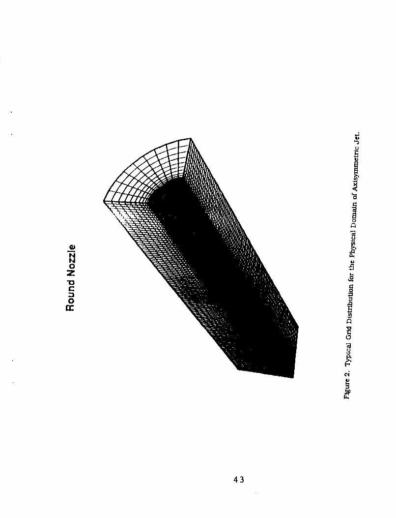
Typical Grid Distribution for the Physical Domain of Axisymmetric ................... 43 Jet.
Comparison of Predicted (3D PNS and SMS) and Measured First ............................ Shock-Cell Characteristics for Supersonic Free Jets.
Typical Convergence History for the Space Marching ,Schemes for .. .. .. .......... ... .... .45 Mach 2.0 and Pj/Pa = 1.45.
Predicted Mach Contours (3D SMS) for Underexpanded Sonic Jet .......................... 46 Operated at DilTerent Pressure Ratios.
Comparisons Between Time-dependent and Space Marching ................................. 47 Solutions in Predicting the Centerline Pressure of Underexpanded Mach 2 Jet and Pj/Pa = 1.45.
Comparison Between Different Turbulence Models (ML and ML-CC) ......................48 Predictions and Measured Centerline Pressure of Underexpanded Mach 2 Jet and PJ/Pa = 1.45.
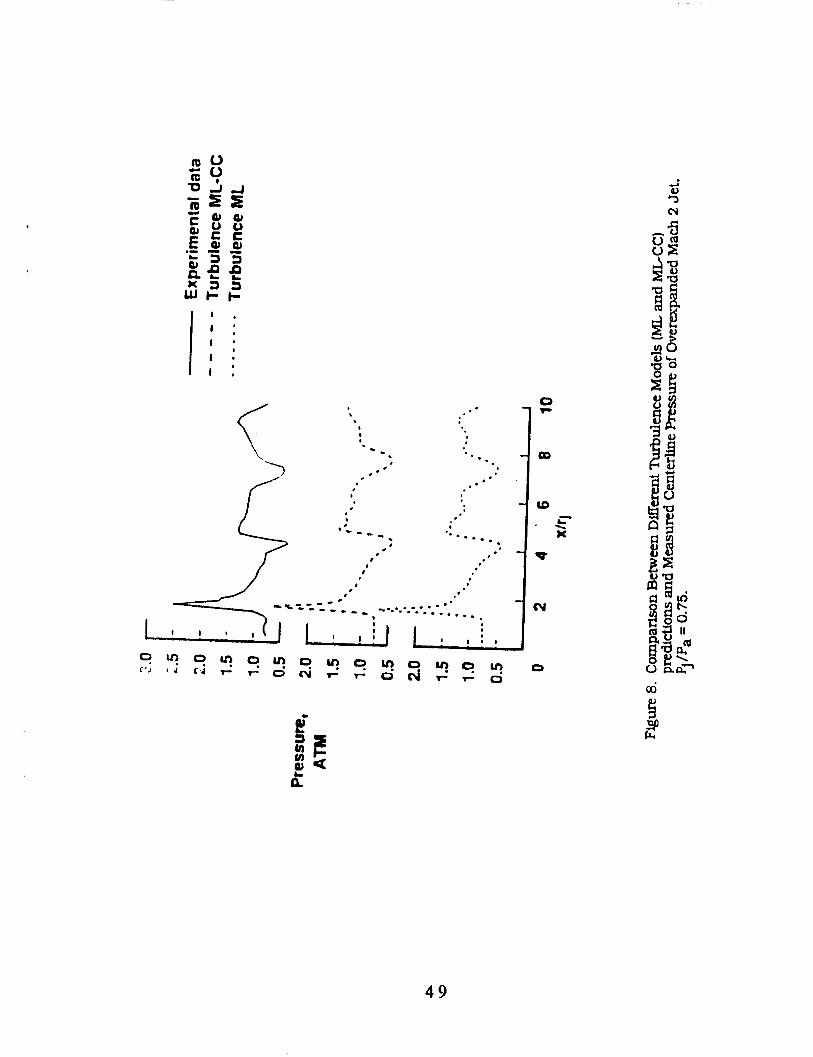
Comparison Between Different Turbulence Models (ML and ML-CC) ...................... 49 Predictions and Measured Centerline Pressure of Overexpanded Mach 2 Jet and Pj /Pa = 1.45.
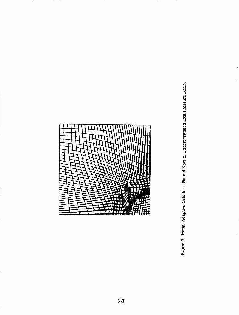
Initial Adaptive Grid for a Round Nomle. Underexpanded Exit Pressure . ........... .. .W Ratio.
Comparison Between Adaptive and Fixed Grid Calculations in . . . .. . . . . . . . . . . . . . . . . . . . . . . . . .5 1 Predicting the Centerline Pressure of Underexpanded Mach 2 Jet.
Three-Dimensional Adaptive Grid Results froni Solving Underexpanded ............. 52 Mach 2. Round Nozzle Using Single Block Strategy.
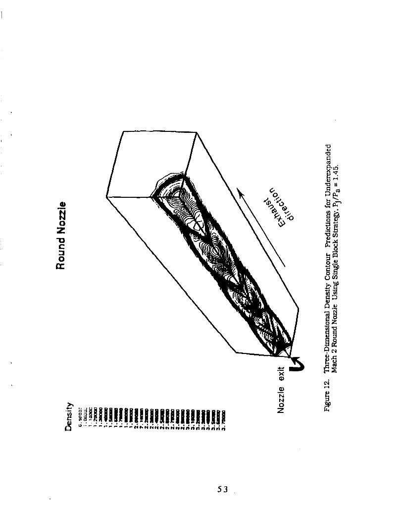
Three-Dimensional Density Contour Predictions for Underexpanded .. . . . . . . . . . . . . . . . .53 Mach 2 Round Nozle Using Single Block Strategy and Pj /Pa = 1.45.
Three-Dimensional Adaptive Grid Results from Solving Underexpanded . . . . . .. . . . .. .54 Mach 2 Round Noizle Using Three Blocks and Pj/P, = 1.45.
Three-Dimensional Density Contour Predictions for Underexpanded .... .. ......... .. .55 Mach 2 Round Nozzle Using Three Blocks and Pj/Pa = 1.45.
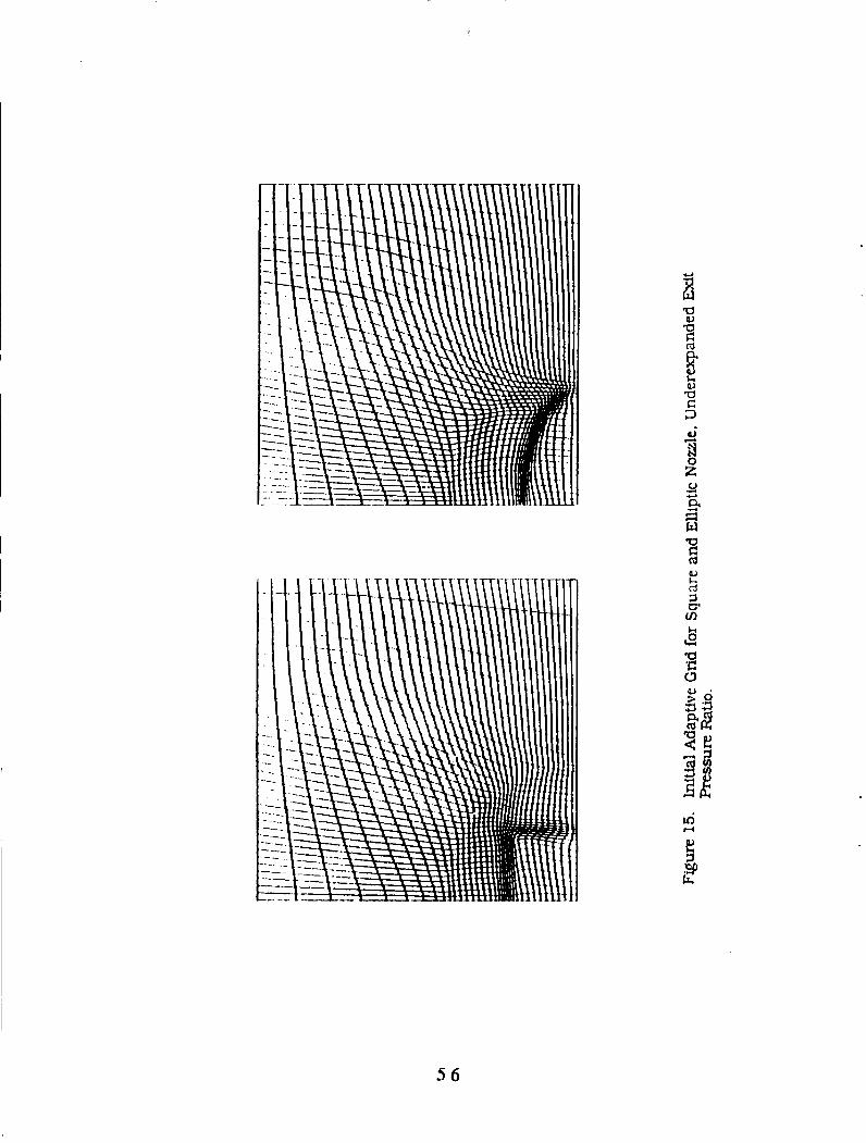
Initial Adaptive Grid for Square and Elliptic Nozzle. Underexpanded Exit ........... 56 Pressure Ratio.
Three-Dimensional Density Contour Predictions for Underexpanded . . . . . . .. .. . . . .. .. ,57 Mach 2 Square Nozzle and Pj/Pa = 1.45.
Comparison Between Adaptive and Fixed Grid Calculations in Predicting . . . . . . . . . . . .58 the Centerline Pressure of Underexpanded Mach 2 Square Nozzle.
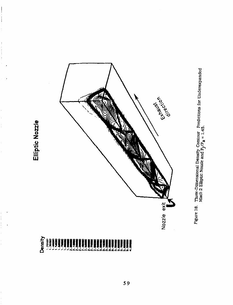
Three-Dimensional Density Contour Predictions for Underexpanded .. ............. .. .59 Mach 2 Elliptic No/zle Pj/Pa = 1.45.
... 111
19.
20.
2 1.
22.
23.
24.
25.
26.
27.
28.
29.
30.
Comparison Between Adaptive and Fixed Grid Calculations in Predicting ............ 60 the Centerline Pressure of Underexpanded Mach 2 Elliptic Nozzle.
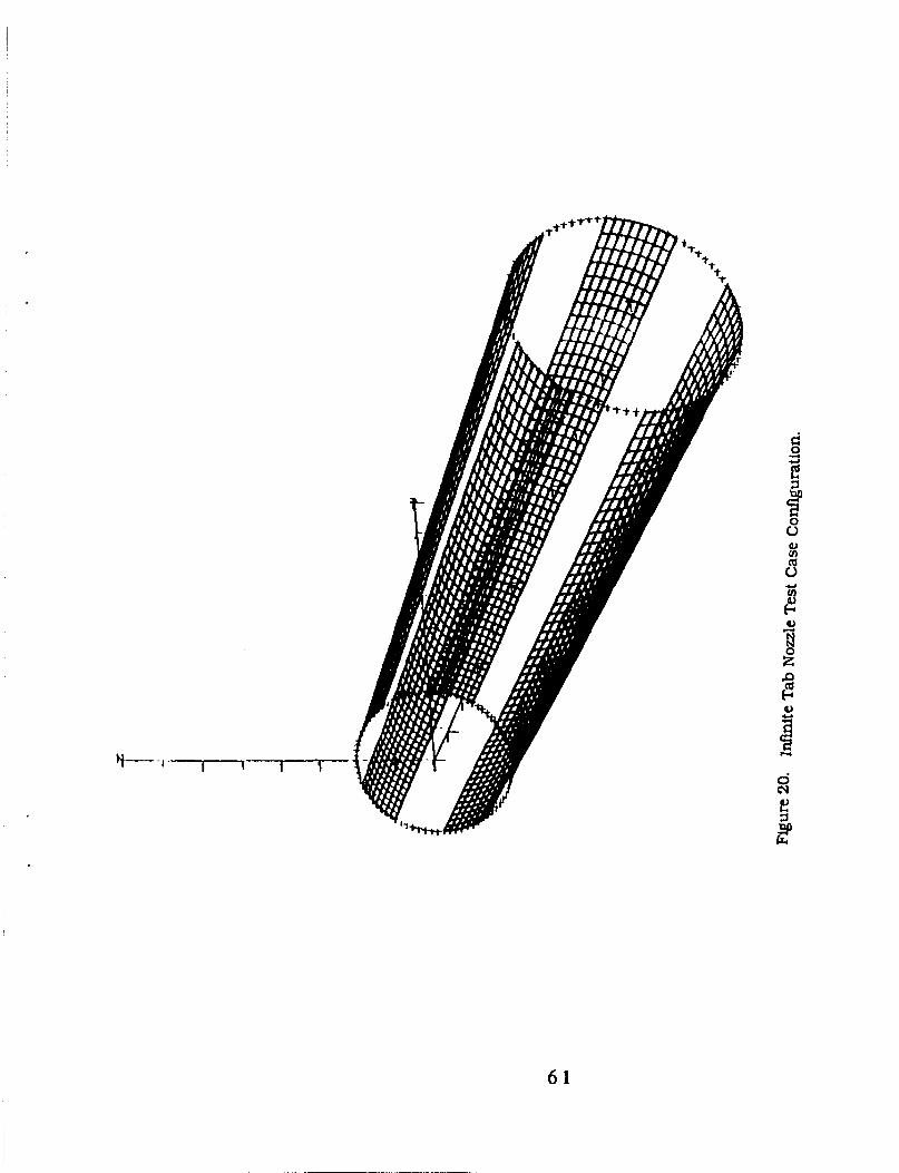
Infinite Tab No7zle Test Case Configuration. ........................................................... 61
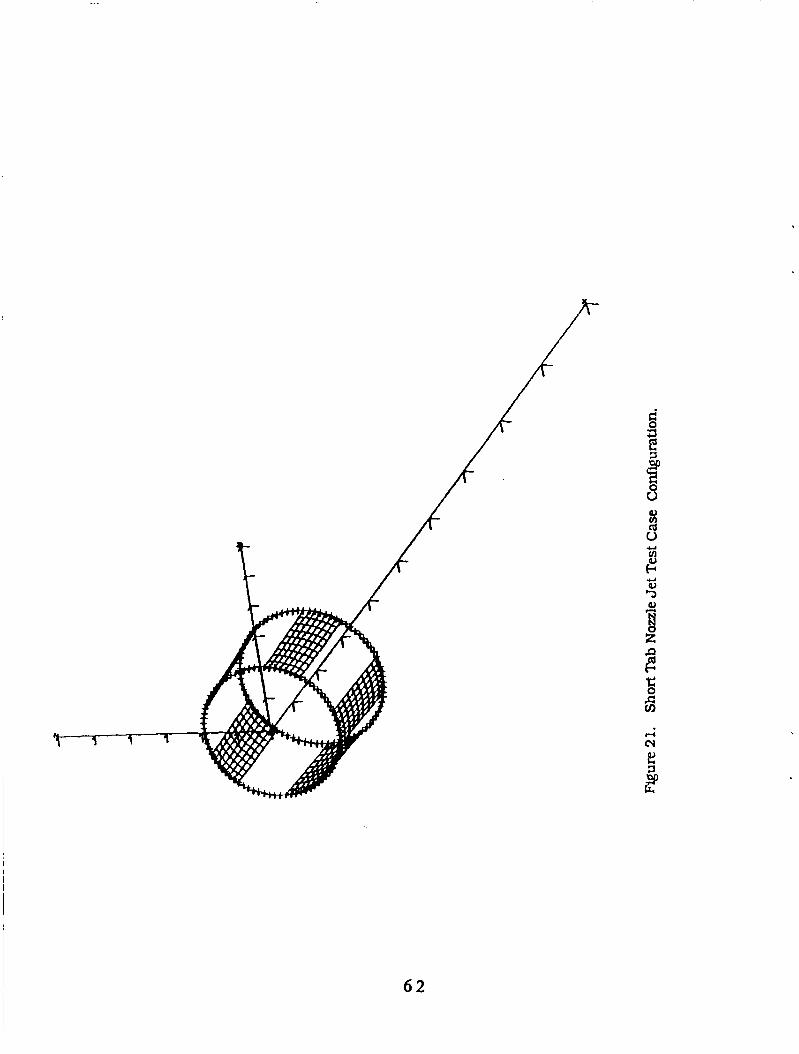
Short Tab Nozzle Jet Test Case C o ~ i ~ u r a t i o n .......................................................... 62
Number of Blocks Required to Solve the 5-Tabs Test Cases.. ................................... .63
a. CFDCodes b. PAB3D-v2 Code
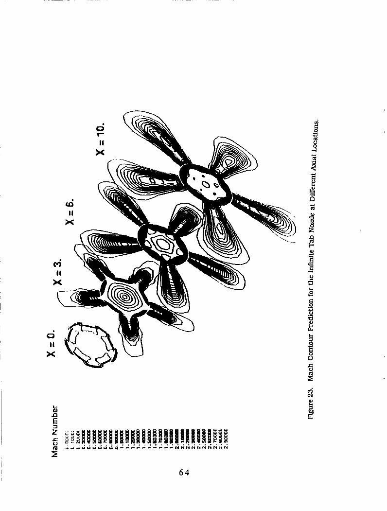
Mach Contour Predictions for the Infinite Tab Nozzle at Different Axial .............. 64 Locations.
Mach Contour Predictions for the Short Tab Nozzle Jet at Different ...................... 65 Axial Locations.
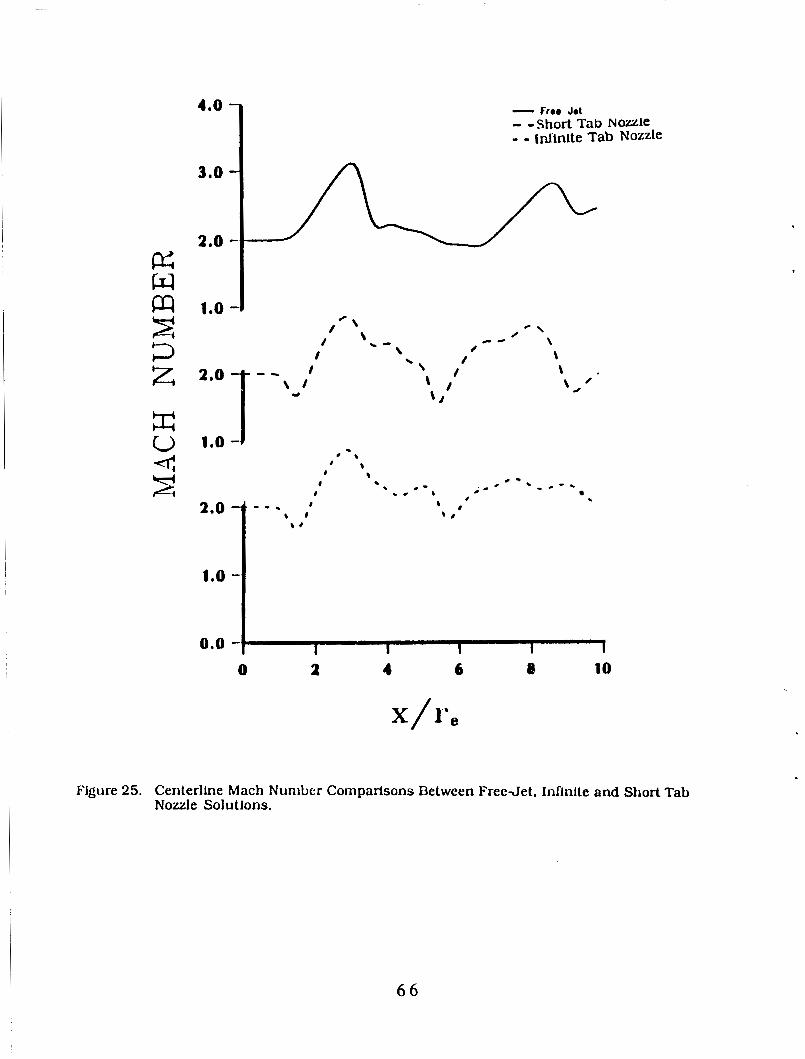
Comparisons Between Free-Jet. Infinite and Short Tab Nozle Centerline ............ 66 Mach Number.
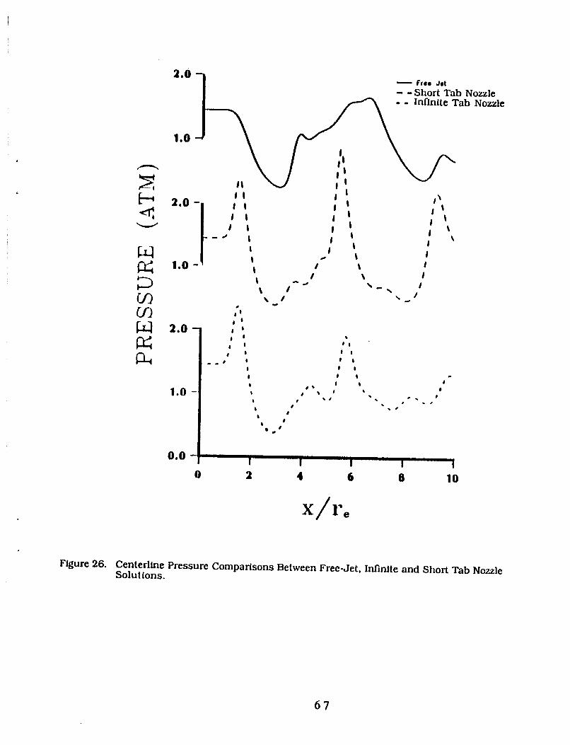
Comparisons Between Free-Jet. Infinite and Short Tab Nolzle Centerline ............ 67 Pressure.
Three-Dimensional Computational Grid for Nonaxisymmetric Aiterbody .......... .68 Test Case.
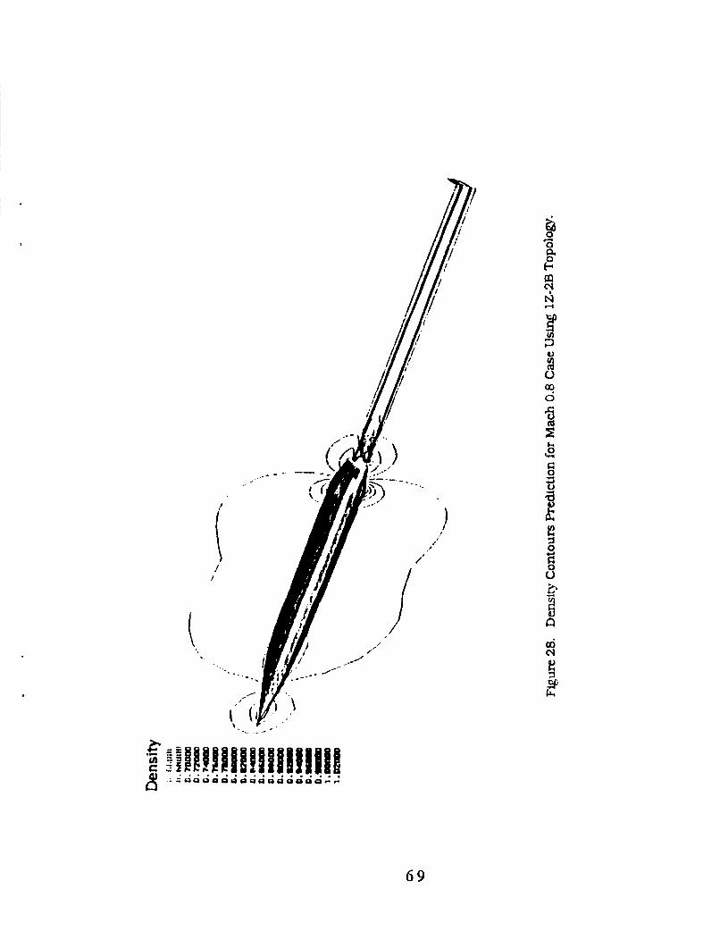
Density Contour Prediction for Mach 0.8 Case Using 1Z-2B Topology. ................... 69
Comparisons Between the Predictions of the Three Different ................................ .70 Multiblock/Multijsone Topologies (1Z-2B. 2Z-2B and 2Z-3B) for Mach 0.8 Test Case.
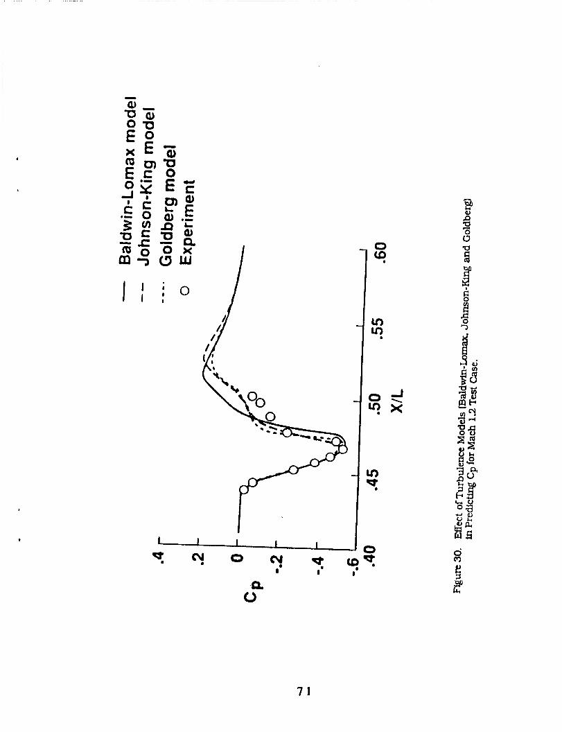
Effect of Turbulence Models (Baldwin-Lomax, Johnson-King and Goldberg) ......... 71 in Predicting Cp for Mach 1.2 Test Case.
i v
A', A:
CCP
CD
Ckleb
CP D
e
E.F.G
E,F,G
F",G"
c
L
Lm
P
Pa
pj
s PNS
RS.T
'e
SMS
X
Nomenclature
Johnson-King modeling constant
Van Driest damping constants
Goldberg turbulence model constants
Cebeci constant
turbulence diffusion constant
Klebanoffs intermittency function
pressure coelficient
jet diameter
total energy
flux vector in x.y and z direction respectively
flux vector in 5.q and [ directions
viscous flwc vector in q and
mixing length scale
afterbody niodel length
dissipation length scale
directions
pressure
free stream pressure
jet centerline pressure
parabolized Navier Stokes
conservative variables
directed surface area of cell face in l&q and [ directions
jet equivalent radius
jet radius
space marching scheme
velocity component in x,y,z directions
coordinate in streamwise direction
V
horizontal coordinate Y
z
Y
5
P
PL
P
z
w
Subscripts
C r
i
e
m
0
S
t
V
W
vertical coordinate
ratio of specific heats
differencing operator in 5.c and q
boundary layer thickness
streamwise direction
circumferential direction
radial direction total dynamic viscosity
turbulent viscosity
laminar viscosity
density
turbulent Reynolds shear stress
vorticity
edge of separation bubble
inner part of boundary layer
laminar
values of quantity where T is a maximum
outer part of boundary layer
edge of the separated region
turbulent
turbulent viscous sublayer region
wall
v i
,
Abstract
This report describes the development and applications of multiblock/
multizone and adaptive grid methodologies for solving the three-dimensional
simplified Navier-Stokes equations. The program was initiated in 1987 focusing on
developing a three-dimensional plume code to simulate the aerodynamic
characteristics of a jet. issuing from nonaxisymmetric noizles. Previously, Abdol-
Hamid et. al. introduced the single zone version of the present code (PAJ33D-vl) where
the parabolized and simplified Navier-Stokes equations were solved. The code was
tested and compared with the experimental data for axisymmetric underexpanded and
overexpanded supersonic jet flows and transonic flow around a nonaxisymmetric
afterbody.
In the present report, adaptive grid and multiblock/multizone approaches are
introduced and applied to external and internal flow problems. These new
implementations increase the capabilities and flexibility of the PAE33D code in solving
flow problems associated with complex geometry.
v i i
1. Introduction
A single block solver can be used efficiently to simulate simple aerodynamic
configurations. Among various methods offered by many researchers, Abdol-Hamid
*2*3 introduced the single block version of PAE33D code to simulate underexpanded and
overexpanded supersonic jets issued from round and rectangular nozzles. Abdol-Hamid
and Compton4 used the PAE33D code to simulate external flow around a nonaxisymmetric
nozzle at a Mach number of 1.2. Pao and Abdol-Hamid5 used the single block with
adaptive grid to simulate underexpanded supersonic jet flows issued from round,
square, and elliptic nomles.
As better computational methods and powerful computers are available in
recent years, computational fluid dynamics (CFI)) has become one of the important
tools in improving aircraft design (6.7). Until recently. the use of CFD was limited to
simple geometries. Future aircraft (fighter or transport) will have very complex
geometries and are difficult to handle with a single zone structured grid. Either
unstructured or multiblock/multizone structured grids are attractive approaches for
solving viscous flow problems with complex configurations. Even though the
unstructured grid is much easier to generate, it requires more computational time and
memory for solving the Navier-Stokes equations per grid point. With the capability of
the supercomputers of today, the multiblock/multizone approach is a flexible method
which can handle very complex configurations.
The advantages in using the multiblock/multizone approach are:
1. Simple grid generation for complex configurations.
2. Flexibility to use a different CFD approach for each block:
a. Numerical technique (space marching algorithms for supersonic flows
and time-dependent algorithms for subsonic and separated flows).
b. Different topology for each block (polar, Cartesian. etc.).
c. Adaptive grid in regions where the dependent variables and their
gradients change their strength and location.
3. Less memory as each zone is solved independently with appropriate
boundary conditions.
This report describes the capabilities of an improved version of the PAE3 3D-vl code
reported in references 1 to 4. This improved code, named PAB 3D-v2. includes options
for three different numerical schemes to solve the simplified Navier-Stokes equations.
The three schemes are: the flux-vector-splitting scheme of van Lee?, the flux-
difference-splitting scheme of Roeg and a modified Roe scheme (space marching
~ c h e m e ) ~ ~ ~ . Four dflerent turbulence model options are also included in PAB 3D-v2.
The first of the four. the Baldwin-Lomax10 model, is a two-layer algebraic model which
follows the pattern adopted by Cebecil
boundary layer thickness. The second, the Johnson and King model12 as extended to
three-dimensional flows by Abid13 and Abid el. al. 14, is a two-layer hybrid eddy-
viscosity Reynolds shear-stress model in which a simplified ordinary differential
equation for the maximum Reynolds shear-stress is solved. The third, the Goldberg
model15 as modified by Goldberg and Chakravarthy16. can be considered as a three-
layer turbulence model where the third layer is used to simulate the separated regions of
the flow. The last is the mixing length turbulence model2 with the option of including a
compressibility correction factor introduced by Cheuch 7. Two diflerent external and
one internal flow problems are used to test the various code capabilities.
but avoids the necessity of determining the
One important problem for CFD applications is the prediction of the shock-cell
structure of underexpanded and overexpanded supersonic jet flows. Understanding the
eITect of shock-cell structure and interaction of a supersonic jet with the external
stream is essential for the design of future aircraft. Also, the no;.zle exit geometry plays
an important role in designing fighter aircraft for maximum maneuverability over a
wide range of Mach numbers18-22. Developing an efficient computational technique is
2
important to fully understand the flow characteristics of these no7zles. At the present
time, there are few codes available to predict the aerodynamics of three-dimensional
shock containing jets. Wolf et. al. developed a three-dimensional code (SCIP3D23) for
analyzing the propulsive jet mixing problem. Anderson and Barber24 also developed a
three-dimensional Parabolized Navier-Stokes procedure for calculating the heated
subsonic and supersonic jet. This code was used to simulate the jet mixing rate for
axisymmetric. rectangular and splayed noizles operated at design conditions. Abdol-
Hamid2v3v4 introduced a space marching scheme, which is based on modifying the Roe's
scheme, to get an accurate solution to the simplified Navier-Stokes equations for
supersonic flows with a single time sweep. This scheme was successfully used to
simulate underexpanded supersonic round and square jet flow p r o b l e n ~ s ~ . ~ . Pao and
Abdol-Hamid5 introduced a new adaptive grid for analyzing the aerodynamic of shock-
containing single jets. They used this technique to simulate round, square. and elliptic
jet flows. The adaptive grid is used to accurately describe the shear layer and detect and
track the movement ofthe shock system for underexpanded supersonic jets. In the
present report, adaptive grid and multiblock capabilities included in PAB 3D-v2 are
utilized to simulate round, square, and elliptic supersonic jet flows.
Another group of underexpanded supersonic jet flow which involving the
internal and external flow regions for a special family of jet nozzle is analyzed in this
report. These examples are designed for showing the flexibility of the PAB3D-v2 code in
handling mixed boundary conditions over a block interface. The nozzle configuration
can be described as a ctrcular pipe section followed by five equally spaced tabs. Each tab
is simply the extension of an arc segment of the circular pipe for a certain length in the
downstream direction. Each arc segment. representing the width of the tab. is 1 / 10 of
the full circle. For this family of configurations, only two grid blocks are needed for
calculations using the PAl33D-v2 code. It is estimated that at least 30 percent of
computer resources are saved by such structural simplicity when compared to typical
3
multiblock codes. Results of analysis using PAI33D-v2 for these nomles are
qualitatively similar to the experimental results obtained by Wlezien et a144 for
nozles with 1. 2. 4 and 8 tabs. In general. the results show that the tab nozzle
configuration allows rapidly establishment of a pressure equilibrium between the
underexpanded jet flow and the ambient free stream. The jet plume is found to have a
higher spreading rate and a lower core flow Mach number as compared to a similarly
underexpanded supersonic jet issuing from a circular nozzle without tabs.
Finally, PAB3D-v2 was used to predict the aerodynamics of an afterbody at
transonic speed. In fighter development programs, a great amount of effort is spent in
analyzing the afterbody flowfield to efficiently integrate the nozzle and airframe. For
analyzing this complex flowfield, computational fluid dynamics is becoming
increasingly useful. Previous applications of computalional fluid dynamics to the
afterbody problem include numerical techniques ranging from panel methods to
Navier-Stokes solver^^^-^^. Abdol-Hamid and Compton4 used four different
numerical algorithms and three different turbulence models to solve the three-
dimensional Navier-Stokes equations for supersonic flow over a nonaxisymmetric
nozzle. Three of the algorithms were contained in the PAI33D-vl and P A E ~ ~ D - V ~ ~ - ~ and
the other in the CFL3D code31.34-36. In the present report. the multiblock/multizone
approach in PAE3 3D-v2 is utilized to simulate the flow over this nonaxisymmetric
n07jsk at a Mach number of 0.8 using a coarse grid. Also, the perfomiance of the three
turbulence models using a fine grid topology in simulating supersonic flow are
compared with experimental data.
2. Governing Eauations
The governing equations under consideration here are the Reynolds-averaged
Simplified Navier-Stokes equations obtained by neglecting all streamwise derivatives,
a/%. of the viscous terms. The resulting simplified Navier-Stokes equations are
written in generalized coordinates and conservation form as
4
where,
P PU PU pu2 + P
Q= pv . E= puv PW PUW e (e + P)u
PV PW PUV PUW
F = $+P , G= pvw PVW pw2 + P (e + P)v (e + Plw
In these equations, p is the density, u. v. and w are the components of the velocity
in the x, y, z directions, respectively, and e is the total internal energy per unit volume.
The pressure, P, is related to the energy by
Y a T - K - + UT,, + V T xy +WT x% P , ax
5
0
rXY Gv= '5yy
TY Z Y a T - K -+ UT x,, + uTYy +WT
p r a Y
Y aT - K-+ UT, +VT yz + wz zz P, as
where
5 = ((x.y.z.t) = Streamwise (marching) direction
q = q(x.y.z.t) = Normal direction
c = c(x.y,z.t) = Spanwise or circumferential direction
J is the Jacobian of the transformation given by
where.
P = PL + PT P = P L
afterbody calculations jet and nozzle calculations
p~ and p~ are the laminar and turbulent viscosity respectively. In the present
investigation. the turbulent viscosity is evaluated using two algebraic turbulence
models which are described subsequently.
6
The Parabolized Navier-Stokes (PNS) equations are obtained from the
governing equations when the unsteady terms are omitted and the following
assumptions are enforced:
1. The streamwise velocity component is everywhere greater than zero.
2. The pressure gradient term in the streamwise direction aP/% is either omitted or treated with other techniques to avoid a complex eigenvalue.
In the present investigation. the technique of Vigneron et. a1.37 is adopted to
suppress the departure solutions associated with the elliptic behavior of the equations.
Vigneron et. a1.37 show that PNS equations are hyperbolic-parabolic provided that the
streamwise convected flw vector is replaced by
E=[pU.puU+ S, w ~ . p v U + ~ , w ~ . p w U + S,wp.(e +P)C]
where
w = 1 MC21
(7)
and, u is a safely faclor to account for the nonlinearity of the governing equations. A
value of 0.95 is used in the present calculations.
3. Turbulence Model2
The Baldwin-Lorna, Johnson-King, and Goldberg I irbi lence models (for wall
boundary problems) and mixing length turbulence models (for shear flow problems) are
briefly described in this section.
7
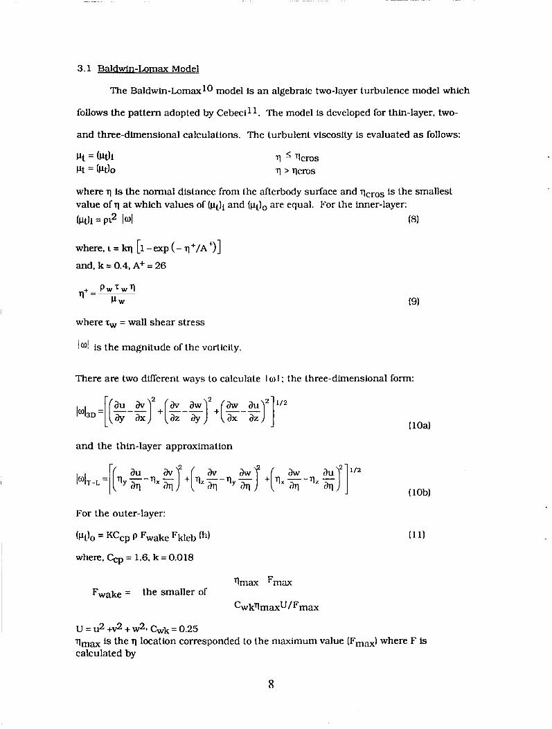
3.1 Baldwin-Lomax Model
The Baldwin-Lomax10 model is an algebraic two-layer turbulence model which
follows the pattern adopted by Cebecil l. The model is developed for thin-layer, two-
and three-dimensional calculations. The turbulent viscosity is evaluated as follows:
where q is the normal distance from the afterbody surface and qcros is the smallest value of q at which values of (pt)i and are equal. For the inner-layer:
(Pt)i = I at (8)
where, I = lq [l -exp (- q+/A+)]
and, k = 0.4, A+ = 26
where T~ = wall shear stress
1 is the magnitude of the vorticity.
There are two dflerent ways to calculate I w I : the three-dimensional form:
and the thin-layer approximation
For the outer-layer:
bt)o = Keep P Fwake Fkleb (h)
where. Qp = 1.6. k = 0.018
qmax Fniax
cw kV m axu / Fmax Fwake = the smaller of
u = U2 +V2 + W2* cwk= 0.25 q m a is the q location corresponded to the maximum value (Fnla) where F is calculated by
8
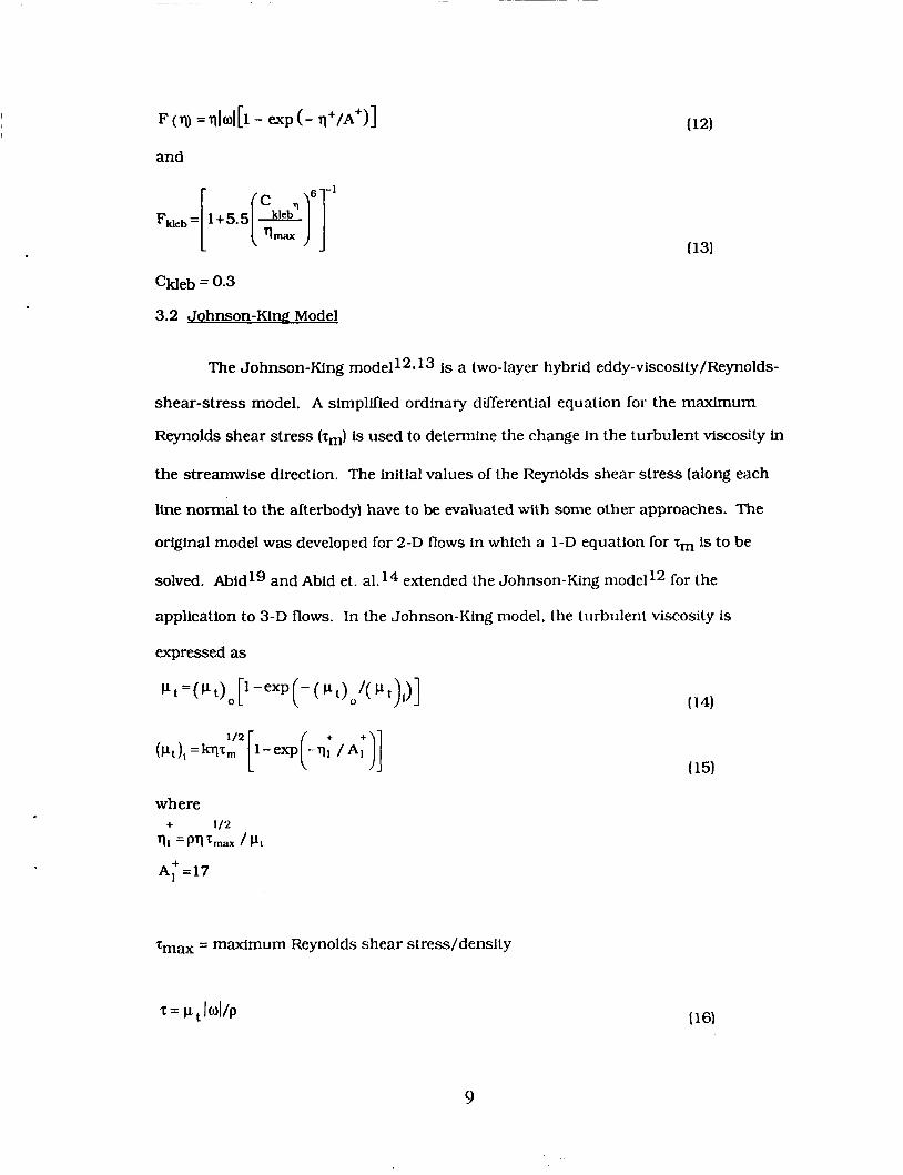
CHeb = 0.3
3.2 Johnson-King Model
The Johnson-King modella* l3 is a two-layer hybrid eddy-viscosity/Reynolds-
shear-stress model. A simplified ordinary differential equation for the maximum
Reynolds shear stress (7,) is used to deterniine the change in the turbulent viscosity in
the streamwise direction. The initial values of the Reynolds shear stress (along each
line normal to the afterbody) have to be evaluated with some other approaches. The
original model was developed for 2-D flows in which a 1-D equation for 'Tm is to be
solved. Abidlg and Abid et. al. l4 extended the Johnson-King niodel12 for the
application to 3-D flows. In the Johnson-King model. the turbulent viscosity is
expressed as
T~~ = maximum Reynolds shear stress/densily
9
The outer eddy viscosity is the same as the one used for the Baldwin-Lomax model
(equation 11) but multiplied by a correction factor Q. However, k takes a value of 0 . 0 1 6 8
as suggested by Abid et. al. 14. The Q factor provides a link between the eddy viscosity
evaluated by equation (16) and Tm. Tm is evaluated by solving the 2-D ordinary
dirrerential equation, which can be written in the following finite volume form:
Wrn 5 u, r, 6 g+-6 g + r = o
where
U, =Rxum +R,,v, +R,w,,
W, =Txum +TYv, +T,w,
where a1 = 0.25. CD = 0.5
Z, = min (0.4 qm. 0.096)
g=z ,
First. the Baldwin-Lomax mode is used to s u p ~ ; . j the initial values for Tnl at each
streamwise location, and Q is set to 1. Then, at the following time steps. equation (17) is
solved for Tm using an upwind-scheme, and o is updated as follows
-1 /2
i
In the region where Q is less than unity. the value of (1 - o"1 (equation 14) is set to zero.
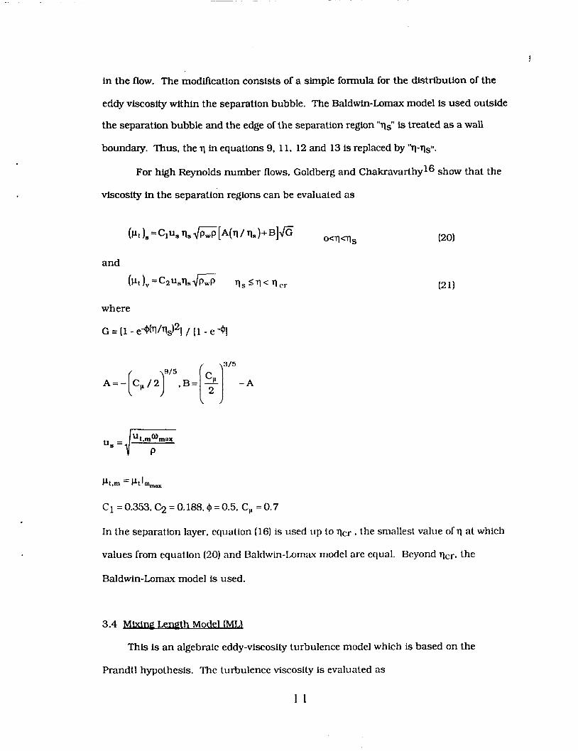
3.3. Goldberg Modification
G01dber-g~~ and Goldberg and Chakravarthyl6 introduced a modification for
boundary layer turbulence models, which is designed to simulate the separation bubble
1 0
!
in the flow. The modification consists of a simple formula for the distribution of the
eddy viscosity within the separation bubble. The Baldwin-Lomax model is used outside
the separation bubble and the edge of the separation region "qg' is treated as a wall
boundary. Thus, the q in equations 9. 11. 12 and 13 is replaced by "q-qsii.
For high Reynolds number flows, Goldberg and Chakravarthy16 show that the
viscosity in the separation regions can be evaluated as
Ft .m = Ptlm,,,=
C1 =0.353. C2=0.188.9=0.5. C, =0.7
In the separation layer, equation (16) is used up to qcr , the smallest value of q at which
values from equation (20) and Baldwin-I,om,zu model are equal. Beyond qcr. the
Baldwin-Lomax model is used.
3.4 Mixing Length Model (ML)
This is an algebraic eddy-viscosity turbulence model which is based on the
Prandtl hypothesis. The turbulence viscosity is evaluated as
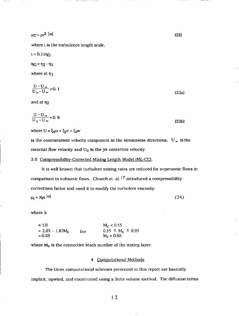
1 1
pT = p 2 14
where L is the turbulence length scale,
L = 0.1 lqc
qc = 172 - ql where at q 1
u -u, =o. 1 u,-u,
and at q2
u-u, u,-u, =o. 9
where U = &u + eyv + &w
is the contravarient velocity component in the streamwise directions, U oo is the
external flow velocity and Uo is the jet centerline velocity.
3.5 ComDressibilitv-Corrected Mixing Length Model IML-CCL.
I t is well known that lurbulent mixing rates are reduced for supersonic flows in
comparison to subsonic flows. Chuech el. al. l7 introduced a compressibility
corrections factor and used it to modify the turbulent viscosity:
pt = KpL 101 (24)
where k
= 1.0 Mc < 0.55 = 2.03 - 1.87Mc for 0.55 s Mc 5: 0.95 = 0.25 MC > 0.95
where Mc is the connective Mach number of the mixing layer.
4. Computational Met hods
The three computational schemes presenled in this report are basically
implicit. upwind, and constructed using a finite volume melhod. The diffusion terms
1 2
are centrally differenced and the inviscid flux terms are upwind differenced in these
schemes. Associating the subscripts i,kj with 5. q, directions, a numerical
approximation to Eq. (1) may be written in the following form:
n+l n+l n+ l n+l n + l n + l
I+-,k.] I---.k.j i .k+-- . j i ,k-- , j i ,k,]+-, 1.k.j---. 2 2 2 2 2 2
(25) (Gi ,k , j ) t + E 1 -E 1 + F 1 -F 1 +G 1 -G * =o
The fluxes at (n + 1 t h e iteration) are linearized as
n n + l - n aE;
F = F +-AQ aQ
n + ~ - n 6 =G +- A Q
aQ
Then, equation (25) is written as,
E 1 n + l I + -. k.] -En+: I - --.k.j ={E+(Q-)+E-(Q+)r . 2 2
- P+(Q-)+E-(Q+)[ i + - - . 2 1 k.j
/ J i+L, k . j 2
*J
I 2
--.k.j
1 3
JI+L, 2
In the present code, two flux-splitting schemes are used to construct the convective flux
terms in equation (26).
The variables Q+, Q- are defined by an upwind biased one parameter
family
These variables can be either the conservative or primitive variables. Also. Q+ and 9-
represent the right and left variables. respectively. in reference to the cell face.
where
A g Q i . k . j = Q i + l . k . j - Q1.k.j. A { Q l . k . j = Q l . k . j - Q i - 1 . k . j
$ = O first order fully upwind
% = - I
$= 1 second order fully upwind
third order biased upwind @ = 1
However, to ensure monotonic interpolation for the third order interpolation in the
vicinity of a shock, a min mod limiter is used as follows:
V Q = min mod (VQ, bAQ)
A Q = min mod (AQ. bVQ)
1 4
3-kg 1-kg
where b is a compression parameter, b = -
It should be mentioned that the splitting procedures are only used for the
inviscid convection parts of the flux vectors (E= and G) . A second order, central
difference is used to represent the dinusion (viscous) terms.
C1=(JZ)*.1-V2(k + 2
At=(JZ) I - -
2
+ - \ B ~ = J 1 +(JSJ 1
3 1 + - 1 - - 2 2
1 1 + -
2
cg =(Ji)
1 5
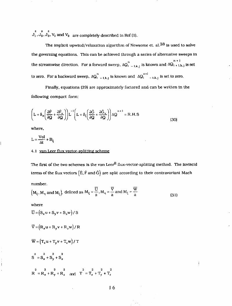
f f f Ji 9 Jz v 53 9 vi and v 2 are completely described in Ref ( 1).
The implicit upwind/relaxation algorithm of Newsome et. al.38 is used to solve
the governing equations. This can be achieved through a series of alternative sweeps in n + l
the streamwise direction. For a forward sweep. - 1,k.j is known and AQi + 1.k.j is set
Finally, equations (29) are approximately factored and can be written in the
following compact form:
where,
Vol L=- At + B6
4.1 van Leer flux vector-s~littinl~ scheme
The first of the two schemes is the van Leers flux-vector-splitting method. The inviscid
terms of the flux vectors (E, F and C ) are split according to their contravariant Mach
number. - - - U V W ( M6, M, and Mg), defined as Mg. = -. M, = - and M5 = - a a a (3 11
where - u =(sxu + s,v + s,w) / s
V = ( R ~ U + R,V + R,W)/R
W = (T,U + T,V + T,W) T
2 2 2 2 s =sx+s,+s,
!
2 2 2 2 2 2 2 2 T =Tx +Ty +T, R = R , + R , + R ,
1 6
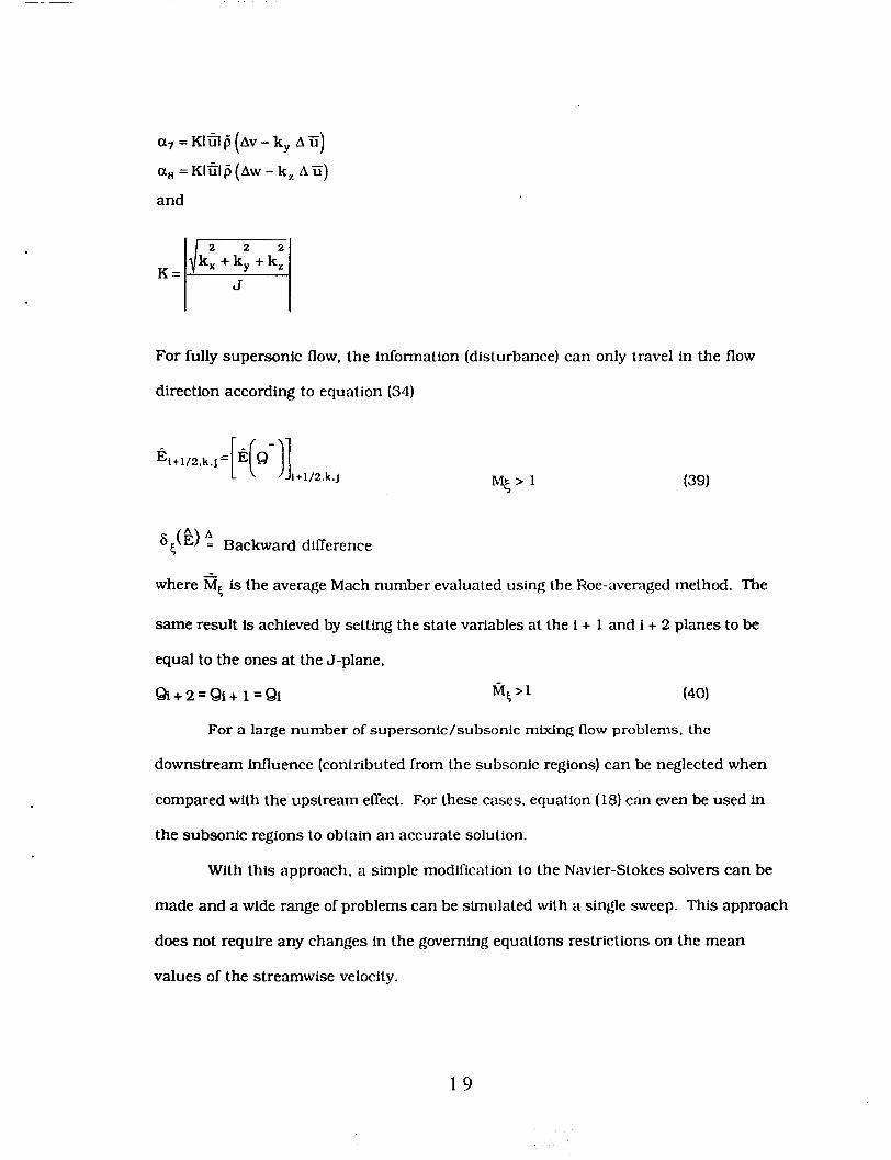
As an example, for supersonfc flows in the x direction
E =E, and E =o. for + -
Mg >1
+ - Mg < - 1 E =o. and E =E. for
and for subsonic flows, -1 e Mg < 1
where
oz f E,,, =_+pa Mg It 1 / 4
7 - u + v + w 2 l Y
t
4.2 Roe 's flux-diuerence -splitling scheme
The second scheme is the Roe's flux-dmerence-splitting method9. which solves the
approximate Riemann problem. For example, the interface flux in the streamwise
direction is evaluated as.
1 7
i
where QL (8-) and QR (Q+) are either primitive or conservative variables to the left and
the right of the cell faces, and A is the Roe-averaged flux Jacobian matrix:
The last term in equation (34) I A I (QR-QL) is defined as:
Berrier. B. L.; Palcza, J. L.; and Richard, G. K.: Nonaxisymmetric Nozle
Technology Program - An Overview. AIAA Paper 77-1225. 1977.
3 8
21. Capone. F. J.: The Nonaxisymmetric Nolxle - It is for Real. AIAA Paper 79-1810.
1979.
22. Stevens, H. L.; Thayer. E. B.: and Fullerton. J. F.: Development of the Multi-
Function 2-D/C-D Nomle. AIAA Paper 8 1 - 149 1, 198 1.
23. Wolf, D. E.; Sinha. N.; and Dash, S . M.: Fully-Coupled Analysis of Jet Mixing
Problems: Three-Dimensional PNS Model, SCIP3D. NASA CR-4 139. 1988.
24. Anderson, 0. L.: and Barber, T. J.: Three Dimensional Analysis of Complex Hot
Exhaust Jets. AIAA Paper 88-3705-CP. 1988.
25. Carlson, John R.: Evaluation and Application of VSAERO to a Nonaxisymmetric
Afterbody with Thrust Vectoring. SAE Technical Paper, 1987.
26. Swanson. R. C. Jr.: Numerical Solutions of the Navier-Stokes Equations for
Transonic Afterbody Flows. NASA TP- 1784. 1980.
27. Swanson. R. C.: Navier-Stokes Solutions for Nonaxisymmetric Nozzle Flows,
AlAA Paper 81-1217, 1981.
28. Deiwert. C. S.: Supersonic Axisynmmetric Flow Over Boattails Containing a
Centered Propulsive Jet. AIAA Journal. Vol. 22. 1984. pp. 1358.-1365.
29. Deiwert. George S . : Anderson, Alison E.: and Nakahasi, Kazuhiro: Theoretical
Analysis of Aircraft Afterbody Flow. Journal of Spacecraft and Rockets. Vol. 24.
1984. pp. 496-503.
30. Deiwert, C. S. and Rothmund. H.: Three-Dimensional Flow Over a Conical
Afterbody Containing Centered Propulsive Jet: A Numerical Solution. AIAA Paper
83- 1709, 1983.
31. Vatsa. V. N.: Thomas. J. L.: and Wedan, €3. W.: Navier-Stokes Computations of
Prolate Spheroids at Angle of Attack. AIAA Paper 87-2627-CP, 1987.
32. Compton. William B.. 111: Thomas, James L.: Abeyounis. William: and Mason,
Mary L.: Transonic Navier-Stokes Solutions of Three-Dimensional Afterbody
Flows. NASA TM-4 1 1 1. 1989.
3 9
33. Abdol-Hamid. K. S.: and Compton. W. B. 111: Supersonic Navier-Stokes
Simulations of Turbulent Afterbody Flows. AIAA Paper 89-2194. 1989.
34. Thomas, J. L.: and Newsome. R. W.: Navier-Stokes Computations of ke-Side Flows
Over Delta Wings. AIAA Paper 86-1049, 1986.
35. Anderson. W. K.; Thomas, J. L.; and van Lee, B.: A Comparison of Finite Volume
F l u Vector Splitlings for Euler Equations. AIAA Paper 85-0122. 1985.
36. van Leer, B.: Thomas. J. L.; Roe. P. L.: and Newsome. R W.: A Comparison of
Numerical Flwc Formulas for the Euler and Navier-Stokes Equations. AIAA paper
87- 1104-CP, 1987.
37. Vigneron, Y. C.: Rakich. J. V.: and Tannehill. J. C.: Calculation of Supersonic
Viscous Flow over Delta Wings with Sharp Subsonic Leading Edges. AIAA Paper
78- 1378, 1987.
38. Newsome. R W.: Walters. R. W.: and Thomas. J. L.: An Efficient Ileration Strategy
for Upwind/Relation Solutions to the Thin-Layer Navier-Stokes Equations. AIAA
Paper 87- 11 13. 1987.
39. Eiseman, P. R.: Alternate Direction Adaptive Grid Generation. AIAA Journal, vol.
23. pp. 55 1-560. 1985.
40. Eiseman. P. R.: and Erlebacher. G.: Grid Generation for the Solution of Partial
DllTerential Equations. ICASE Report No. 87-57. NASA CR- 178365, 1987.
41. Eiseman. P. R.: Adaptive Grid Generation, Computer Methods in Applied
Mechanics and Engineering, vol. 64, pp 32 1-376, 1987.
42. Love, E. S.; Grigsby. L. P.: Lee, L. P.: and Woodling, M. J.: Experimental and
Theoretical Studies of Axisymmetric Free Jets. NASA TR-R6. 1959.
43. Norum. T. D.: and Seiner, J. M.: Measurements of Mean Static Pressure and Far
Field Acoustics of Shock-containing Supersonic Jets. NASA TM-8452 1 , 1984.
44. Wlezien, R. W.: and Kibens. V.: Influence of Nozzle Asymmetry on Supersonic Jets.
AIAA Journal. vol. 26. no. 1 . pp. 27-33. 1988.
4 0
45. Pulnam. Lawrence E.; and Mercer, Charles E.: Pitol-Pressure Measurements in
Flow Fields Behind a Rectangular Nozzle with Exhaust Jet for Free-Stream Mach
Numbers of 0.00. 0.60. and 1.20. NASA TM-88990. 1986.
4 1
N a c 0 N
0 13
4 2
aJ M 0 z 'D t 5 0 a
k E
4 3
u? 9
5 s l-
U U
9
z l-
U lZ
0 or
4 4
t I I I 1 I I I I I 4 I I I I I I I 1 I I I I I I I I I I I I I I I I 1 1 1 I I
0 0 P
0 0 Pa
E 0 'L
Q, N E
L. I
0 0 r
0
0 0 m 3
i? 3 3:
0
4 5
0
II
0 4 II d
e, 3
k e
4 6
2 .o
1.5
1 .o
0.5
2.0
1.5
1 .o
0.5
0.0
-
-
-
-
c - I \
I \
f \
I \ I \ - -1 I \
\ I \ \ I \
\ I \ /
I \ \ v \ \ I I I
\ ' \ 1' \ \ ' \ I \ \ I \ I '-. \ I \ I
\ I \ \ I \
\ I
I I 1 0 5 10 15
E'lgitrc 6. Coriiparlsoris Dclwccri Time-dependent and Space Marclilng Solulloris In Pretllcllrig l l ie Cerilerllrie Pressure of Uiiderexparitlt:d Mach 2 .Jets and €'j/fJa = 1.45.
4 7
* - - - - . - - I
- - - - - a
_- - - I
* - ' - - - _
* - '--':* ,- - -,- - -1
1
0 *
0 m
0 e- NbC
0 r
1 ,
1 :
' : I : I *
4 9
a 3
5 0
n
2.0
1.5
1.0
0.5
2.0
1.5
1.0
0.5
0.0
- f i r e d Grid
0 5 10 15 20
Q I J ~ ~ 10. Comparlson Between Adapllve and Fixed Crld Calculations In Predlctlng lhe Centerline Pressure of Underexpanded Mach 2 Jet.
5 1
0
0 2 1 P C 3 0 a
.- c. X 5 hi a, N - N 0 z
5 2
0 2 P C 3 0 U
Q,
Q, N N 0
-
z
53
Q,
0 z P c 3 0 U
a
t. .- x -5 0,
0, N N
- 0 z
5 4
5 5
B U c k
0 a c 3
Q) k (3 7 ET cn
5 6
d,
0 z
N 0 z
J e k 6, U c 3
5 7
2*o 1
2.0 -
1.5 -.,
1.0 -
0.5 -
- f ired Grid - - Adoptive Grid
I I
I t I '1 I I ' I 1 I I I
\ c \ I \ I t ' I L I \ I L I \ I \ I - \ I \ I b
\ \ I\- \
\ I \ \ I \ \ I \ \ I \ \ I \ \ I \ \ I \ \ I \
1. \I
I I I I I
0 5 10 15 20
Flgirre 17. Comparison Between Adapllve and Flxed Grid Calculations In Predlcllng lhe Cenlerllne Pressure of Underexpanded Mach 2 Square N w l e and Pj/Pa =; 1.45
5 8
a, a, N N 0
-
z
5 9
n
2 4 W
2.0
1.5
1 .o
0.5
7 - Fixod Grid
0.5
0.0
I I I I
\ I
I \ \ \ \ I
I \ \ \ I \ I
\ 1 4 -\ \ I \ ! I \ \ I \ \ I \ \ I \ \ ( \ \ I \ I \ I \ I
I I I I I
0 S 10 15 20
F4gi~t-e 19. Coniparlsori Between Aidaptlvc and Flxed Grld Calciilatlons I n Predlctlng the Cenlerllric Pressure of Underexpanded Mach 2 Elllptk Noule and Pj/Pa =; 1.45.
60
Y-- 7-
6 1
0 CJ
6 2
n P
0 c,
6 3
0 11
k
0 a c, d 8
6 4
ci II K
d I I K
6 5
.
0 2 4 6 a 10
Flgure 25. Centerllne Mach Nuniber Coniparfsons Between FrecJet, Infinite and Short Tab Noule Solutions.
Figure 26. Centerlhe Pressure Comparisons Between Free-Jet, Infinite and Short Tab Nozzle Solutions.
6 7
?
h P 0 P b
6 8
f
'. I
tl 1 0 c,
0
6 9
pc
0.4
0.2
00.0
-0.2
-0.4
-0.6
h \ 0 d \o' 0
- 12-20
- - 22-28
- 0 22-30
EXPERIMENTAL OATA
0.40 0.45 0.50 0.55 0.60
Flgiire 29. Cornparlsons Between the Predlctlons of lhe Three Dlflerent Miilllblock/Mulll~oi~~ Topologles (12-2B. 2Z-2;U and 2Z-3U1 for Mach 0.8 Test Case.
70
I '
.
0 (D
a 2
n $
> t
7 1
Report Documentation Page 1 . Repon No.
NASA CR-182032
2. Government Accession No.
7. Authorlsl
!7. Key Words (Suggested by AuthorWI
Khaled S. Abdol-Hamid
18. Distribution Statement
- 9. Performing Organization Name and Address
Analytical Services and Materials, Inc. 107 Research Drive Hampton, VA 23666
Propulsion Aerodynamics Tur b ul en ce Mode 1 s
2. Sponsoring Agency Name and Address
National Aeronautics and Space Administration Langley Research Center Hampton, VA 23665-5225
Subject Category 02
3. Recipient's Catalog No.
19. Security Classif. (of this report) 20. Security Classif. (of this page)
5. Report Date
September 1990 6. Performing Organization Code
21 No. of pages 22. Price
-. 8. Performing Organization Report No.
- 10. Work Unit No.
505-68-91-06 11. Contract or Grant No.
NAS1-18599 13. Type of Report and Period Covered
Contractor Report 14. Sponsoring Agency Code
5. Supplementary Notes
Langley Technical Monitor: Bobby L . Berrier Final Report
6. Abstract
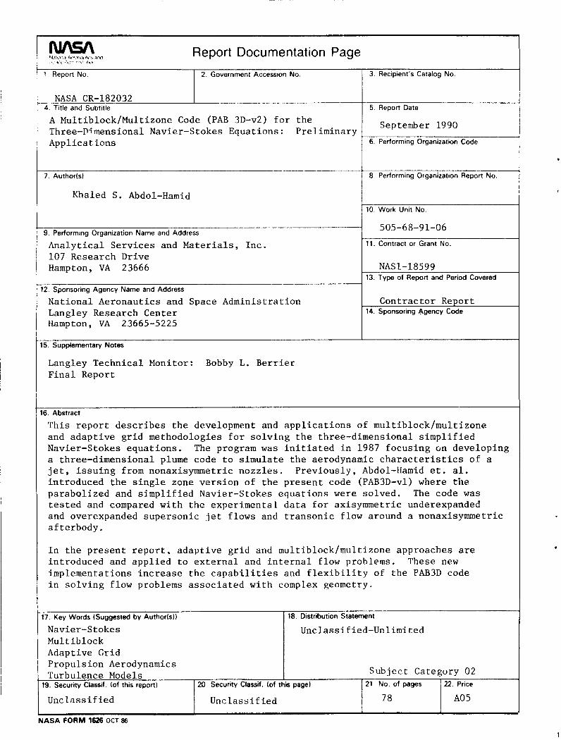
This report describes the development and applications of multiblock/multizone and adaptive grid methodologies for solving the three-dimensional simplified Navier-Stokes equations. The program was initiated in 1987 focusing on developing a three-dimensional plume code to simulate the aerodynamic characteristics of a jet, issuing from nonaxisymmetric nozzles. Previously, Abdol-Hamid et. al. introduced the single zone version of the present code (PAB3D-vl) where the parabolized and simplified Navier-Stokes equations were solved. The code was tested and compared with the experimental data for axisymmetric underexpanded and overexpanded supersonic jet flows and transonic flow around a nonaxisymmetric afterbody.
In the present report, adaptive grid and multiblock/multizone approaches are introduced and applied to external and internal flow problems. These new implementations increase the capabilities and flexibility of the PAB3D code in solving flow problems associated with complex geometry.