87
Load and Resistance Factor Design (LRFD) for Deep Foundations NATIONAL COOPERATIVE HIGHWAY RESEARCH PROGRAM NCHRP REPORT 507
| Date post: | 20-Oct-2015 |
| Category: |
Documents |
| Upload: | yoshua-yang |
| View: | 70 times |
| Download: | 8 times |
Load and Resistance FactorDesign (LRFD) forDeep Foundations
NATIONALCOOPERATIVE HIGHWAYRESEARCH PROGRAMNCHRP
REPORT 507

TRANSPORTATION RESEARCH BOARD EXECUTIVE COMMITTEE 2004 (Membership as of January 2004)
OFFICERSChair: Michael S. Townes, President and CEO, Hampton Roads Transit, Hampton, VA Vice Chair: Joseph H. Boardman, Commissioner, New York State DOTExecutive Director: Robert E. Skinner, Jr., Transportation Research Board
MEMBERSMICHAEL W. BEHRENS, Executive Director, Texas DOTSARAH C. CAMPBELL, President, TransManagement, Inc., Washington, DCE. DEAN CARLSON, Director, Carlson Associates, Topeka, KSJOHN L. CRAIG, Director, Nebraska Department of RoadsDOUGLAS G. DUNCAN, President and CEO, FedEx Freight, Memphis, TNGENEVIEVE GIULIANO, Director, Metrans Transportation Center and Professor, School of Policy, Planning, and Development, USC,
Los AngelesBERNARD S. GROSECLOSE, JR., President and CEO, South Carolina State Ports AuthoritySUSAN HANSON, Landry University Professor of Geography, Graduate School of Geography, Clark UniversityJAMES R. HERTWIG, President, Landstar Logistics, Inc., Jacksonville, FLHENRY L. HUNGERBEELER, Director, Missouri DOTADIB K. KANAFANI, Cahill Professor of Civil Engineering, University of California, Berkeley RONALD F. KIRBY, Director of Transportation Planning, Metropolitan Washington Council of GovernmentsHERBERT S. LEVINSON, Principal, Herbert S. Levinson Transportation Consultant, New Haven, CTSUE MCNEIL, Director, Urban Transportation Center and Professor, College of Urban Planning and Public Affairs, University of
Illinois, ChicagoMICHAEL D. MEYER, Professor, School of Civil and Environmental Engineering, Georgia Institute of TechnologyKAM MOVASSAGHI, Secretary of Transportation, Louisiana Department of Transportation and DevelopmentCAROL A. MURRAY, Commissioner, New Hampshire DOTJOHN E. NJORD, Executive Director, Utah DOTDAVID PLAVIN, President, Airports Council International, Washington, DCJOHN REBENSDORF, Vice President, Network and Service Planning, Union Pacific Railroad Co., Omaha, NEPHILIP A. SHUCET, Commissioner, Virginia DOTC. MICHAEL WALTON, Ernest H. Cockrell Centennial Chair in Engineering, University of Texas, AustinLINDA S. WATSON, General Manager, Corpus Christi Regional Transportation Authority, Corpus Christi, TX
MARION C. BLAKEY, Federal Aviation Administrator, U.S.DOT (ex officio)SAMUEL G. BONASSO, Acting Administrator, Research and Special Programs Administration, U.S.DOT (ex officio)REBECCA M. BREWSTER, President and COO, American Transportation Research Institute, Smyrna, GA (ex officio)GEORGE BUGLIARELLO, Chancellor, Polytechnic University and Foreign Secretary, National Academy of Engineering (ex officio)THOMAS H. COLLINS (Adm., U.S. Coast Guard), Commandant, U.S. Coast Guard (ex officio)JENNIFER L. DORN, Federal Transit Administrator, U.S.DOT (ex officio)ROBERT B. FLOWERS (Lt. Gen., U.S. Army), Chief of Engineers and Commander, U.S. Army Corps of Engineers (ex officio)EDWARD R. HAMBERGER, President and CEO, Association of American Railroads (ex officio)JOHN C. HORSLEY, Executive Director, American Association of State Highway and Transportation Officials (ex officio)RICK KOWALEWSKI, Deputy Director, Bureau of Transportation Statistics, U.S.DOT (ex officio)WILLIAM W. MILLAR, President, American Public Transportation Association (ex officio) MARY E. PETERS, Federal Highway Administrator, U.S.DOT (ex officio)SUZANNE RUDZINSKI, Director, Transportation and Regional Programs, U.S. Environmental Protection Agency (ex officio)JEFFREY W. RUNGE, National Highway Traffic Safety Administrator, U.S.DOT (ex officio)ALLAN RUTTER, Federal Railroad Administrator, U.S.DOT (ex officio)ANNETTE M. SANDBERG, Federal Motor Carrier Safety Administrator, U.S.DOT (ex officio)WILLIAM G. SCHUBERT, Maritime Administrator, U.S.DOT (ex officio)ROBERT A. VENEZIA, Program Manager of Public Health Applications, National Aeronautics and Space Administration (ex officio)
NATIONAL COOPERATIVE HIGHWAY RESEARCH PROGRAM
Transportation Research Board Executive Committee Subcommittee for NCHRPMICHAEL S. TOWNES, Hampton Roads Transit, Hampton, VA
(Chair)JOSEPH H. BOARDMAN, New York State DOTGENEVIEVE GIULIANO, University of Southern California,
Los Angeles
JOHN C. HORSLEY, American Association of State Highway and Transportation Officials
MARY E. PETERS, Federal Highway Administration ROBERT E. SKINNER, JR., Transportation Research BoardC. MICHAEL WALTON, University of Texas, Austin
T R A N S P O R T A T I O N R E S E A R C H B O A R DWASHINGTON, D.C.
2004www.TRB.org
NATIONAL COOPERATIVE HIGHWAY RESEARCH PROGRAM
NCHRP REPORT 507
Research Sponsored by the American Association of State Highway and Transportation Officials in Cooperation with the Federal Highway Administration
SUBJECT AREAS
Bridges, Other Structures, and Hydraulics and Hydrology • Soils, Geology and Foundations
Load and Resistance FactorDesign (LRFD) forDeep Foundations
SAMUEL G. PAIKOWSKY
Geotechnical Engineering Research Laboratory
Department of Civil & Environmental Engineering
University of Massachusetts
Lowell, MA
WITH CONTRIBUTIONS BY:BJORN BIRGISSON, MICHAEL MCVAY, THAI NGUYEN
University of Florida
Gainesville, FL
CHING KUO
Geostructures, Inc.
Tampa, FL
GREGORY BAECHER
BILAL AYYUB
University of Maryland
College Park, MD
KIRK STENERSEN
KEVIN O’MALLEY
University of Massachusetts
Lowell, MA
LES CHERNAUSKAS
Geosciences Testing and Research, Inc.
N. Chelmsford, MA
MICHAEL O’NEILL
University of Houston
Houston, TX

NATIONAL COOPERATIVE HIGHWAY RESEARCH PROGRAM
Systematic, well-designed research provides the most effectiveapproach to the solution of many problems facing highwayadministrators and engineers. Often, highway problems are of localinterest and can best be studied by highway departmentsindividually or in cooperation with their state universities andothers. However, the accelerating growth of highway transportationdevelops increasingly complex problems of wide interest tohighway authorities. These problems are best studied through acoordinated program of cooperative research.
In recognition of these needs, the highway administrators of theAmerican Association of State Highway and TransportationOfficials initiated in 1962 an objective national highway researchprogram employing modern scientific techniques. This program issupported on a continuing basis by funds from participatingmember states of the Association and it receives the full cooperationand support of the Federal Highway Administration, United StatesDepartment of Transportation.
The Transportation Research Board of the National Academieswas requested by the Association to administer the researchprogram because of the Board’s recognized objectivity andunderstanding of modern research practices. The Board is uniquelysuited for this purpose as it maintains an extensive committeestructure from which authorities on any highway transportationsubject may be drawn; it possesses avenues of communications andcooperation with federal, state and local governmental agencies,universities, and industry; its relationship to the National ResearchCouncil is an insurance of objectivity; it maintains a full-timeresearch correlation staff of specialists in highway transportationmatters to bring the findings of research directly to those who are ina position to use them.
The program is developed on the basis of research needsidentified by chief administrators of the highway and transportationdepartments and by committees of AASHTO. Each year, specificareas of research needs to be included in the program are proposedto the National Research Council and the Board by the AmericanAssociation of State Highway and Transportation Officials.Research projects to fulfill these needs are defined by the Board, andqualified research agencies are selected from those that havesubmitted proposals. Administration and surveillance of researchcontracts are the responsibilities of the National Research Counciland the Transportation Research Board.
The needs for highway research are many, and the NationalCooperative Highway Research Program can make significantcontributions to the solution of highway transportation problems ofmutual concern to many responsible groups. The program,however, is intended to complement rather than to substitute for orduplicate other highway research programs.
Note: The Transportation Research Board of the National Academies, theNational Research Council, the Federal Highway Administration, the AmericanAssociation of State Highway and Transportation Officials, and the individualstates participating in the National Cooperative Highway Research Program donot endorse products or manufacturers. Trade or manufacturers’ names appearherein solely because they are considered essential to the object of this report.
Published reports of the
NATIONAL COOPERATIVE HIGHWAY RESEARCH PROGRAM
are available from:
Transportation Research BoardBusiness Office500 Fifth Street, NWWashington, DC 20001
and can be ordered through the Internet at:
http://www.national-academies.org/trb/bookstore
Printed in the United States of America
NCHRP REPORT 507
Project 24-17 FY’99
ISSN 0077-5614
ISBN 0-309-08796-1
Library of Congress Control Number 2004107693
© 2004 Transportation Research Board
Price $31.00
NOTICE
The project that is the subject of this report was a part of the National Cooperative
Highway Research Program conducted by the Transportation Research Board with the
approval of the Governing Board of the National Research Council. Such approval
reflects the Governing Board’s judgment that the program concerned is of national
importance and appropriate with respect to both the purposes and resources of the
National Research Council.
The members of the technical committee selected to monitor this project and to review
this report were chosen for recognized scholarly competence and with due
consideration for the balance of disciplines appropriate to the project. The opinions and
conclusions expressed or implied are those of the research agency that performed the
research, and, while they have been accepted as appropriate by the technical committee,
they are not necessarily those of the Transportation Research Board, the National
Research Council, the American Association of State Highway and Transportation
Officials, or the Federal Highway Administration, U.S. Department of Transportation.
Each report is reviewed and accepted for publication by the technical committee
according to procedures established and monitored by the Transportation Research
Board Executive Committee and the Governing Board of the National Research
Council.

The National Academy of Sciences is a private, nonprofit, self-perpetuating society of distinguished schol-ars engaged in scientific and engineering research, dedicated to the furtherance of science and technology and to their use for the general welfare. On the authority of the charter granted to it by the Congress in 1863, the Academy has a mandate that requires it to advise the federal government on scientific and techni-cal matters. Dr. Bruce M. Alberts is president of the National Academy of Sciences.
The National Academy of Engineering was established in 1964, under the charter of the National Acad-emy of Sciences, as a parallel organization of outstanding engineers. It is autonomous in its administration and in the selection of its members, sharing with the National Academy of Sciences the responsibility for advising the federal government. The National Academy of Engineering also sponsors engineering programs aimed at meeting national needs, encourages education and research, and recognizes the superior achieve-ments of engineers. Dr. William A. Wulf is president of the National Academy of Engineering.
The Institute of Medicine was established in 1970 by the National Academy of Sciences to secure the services of eminent members of appropriate professions in the examination of policy matters pertaining to the health of the public. The Institute acts under the responsibility given to the National Academy of Sciences by its congressional charter to be an adviser to the federal government and, on its own initiative, to identify issues of medical care, research, and education. Dr. Harvey V. Fineberg is president of the Institute of Medicine.
The National Research Council was organized by the National Academy of Sciences in 1916 to associate the broad community of science and technology with the Academy’s purposes of furthering knowledge and advising the federal government. Functioning in accordance with general policies determined by the Acad-emy, the Council has become the principal operating agency of both the National Academy of Sciences and the National Academy of Engineering in providing services to the government, the public, and the scientific and engineering communities. The Council is administered jointly by both the Academies and the Institute of Medicine. Dr. Bruce M. Alberts and Dr. William A. Wulf are chair and vice chair, respectively, of the National Research Council.
The Transportation Research Board is a division of the National Research Council, which serves the National Academy of Sciences and the National Academy of Engineering. The Board’s mission is to promote innovation and progress in transportation through research. In an objective and interdisciplinary setting, the Board facilitates the sharing of information on transportation practice and policy by researchers and practitioners; stimulates research and offers research management services that promote technical excellence; provides expert advice on transportation policy and programs; and disseminates research results broadly and encourages their implementation. The Board’s varied activities annually engage more than 5,000 engineers, scientists, and other transportation researchers and practitioners from the public and private sectors and academia, all of whom contribute their expertise in the public interest. The program is supported by state transportation departments, federal agencies including the component administrations of the U.S. Department of Transportation, and other organizations and individuals interested in the development of transportation. www.TRB.org
www.national-academies.org

COOPERATIVE RESEARCH PROGRAMS STAFF FOR NCHRP REPORT 507
ROBERT J. REILLY, Director, Cooperative Research ProgramsCRAWFORD F. JENCKS, Manager, NCHRPDAVID B. BEAL, Senior Program OfficerEILEEN P. DELANEY, Managing EditorHILARY FREER, Associate Editor
NCHRP PROJECT 24-17 PANELField of Design—Area of Bridges, Other Structures, and Hydraulics and Hydrology
TERRY SHIKE, P.E., David Evans and Associates, Inc., Salem, Oregon (Chair)PAUL F. BAILEY, P.E., New York State DOTRICHARD BARKER, P.E., Blacksburg, VirginiaJERRY A. DIMAGGIO, P.E., FHWAWILLIAM S. FULLERTON, P.E., Montana DOTROBERT E. KIMMERLING, P.E., PanGeo, Inc., Seattle, WashingtonMARK J. MORVANT, P.E., Louisiana DOTD, Louisiana Transportation Research CenterPAUL PASSE, P.E., PSI, Tampa, FloridaJEFF SIZEMORE, P.E., South Carolina DOTCARL EALY, FHWA Liaison RepresentativeG. P. JAYAPRAKASH, TRB Liaison Representative
AUTHOR ACKNOWLEDGMENTSThe presented research was sponsored by the American Associ-
ation of State Highway and Transportation Officials (AASHTO),under project 24-17, in cooperation with the Federal HighwayAdministration (FHWA). The panel of the research project isacknowledged for their comments and suggestions. The interest,support, and suggestions of Mr. David Beal of the NCHRP arehighly appreciated. Messrs. Jerry DiMaggio, Al DiMillio, and CarlEaly of the FHWA are acknowledged for their concern and sup-port. Dr. Gregory Baecher and Dr. Bilal Ayyub from the Univer-sity of Maryland contributed to sections 1.3.1 through 1.3.4, sec-tion 1.4.3.4, sections 2.6.1 through 2.6.3, and section 3.3, andperformed the calculations of the presented resistance factors
based on FORM. Dr. Mike McVay, Dr. Bjorn Birgisson, and Mr.Thai Nguyen of the University of Florida, and Dr. Ching Kuo ofGeostructures compiled the static analyses databases and carriedout the analyses related to the material presented in sections 2.1.1,2.1.2, 2.3.1, 2.5, 3.1.2, and 3.1.4. Dr. Frank Rausche of Goble,Rausche, Likins (GRL) and Associates provided the data pertain-ing to the evaluation of GRLWEAP as the WEAP method fordynamic pile capacity evaluation. Mr. Kirk Stenersen researchedthe performance of the dynamic analyses as part of his graduatestudies at the University of Massachusetts Lowell. The help of Ms.Mary Canniff and Ms. Laural Stokes in the preparation of the man-uscript is appreciated.
This report contains the findings of a study to develop resistance factors for drivenpile and drilled shaft foundations. These factors are recommended for inclusion in Sec-tion 10 of the AASHTO LRFD Bridge Design Specifications to reflect current bestpractice in geotechnical design and construction. The report also provides a detailedprocedure for calibrating deep foundation resistance. The material in this report will beof immediate interest to bridge engineers and geotechnical engineers involved in thedesign of pile and drilled shaft foundations.
Full implementation of the AASHTO LRFD Bridge Design Specifications for deepfoundations is hampered by provisions that are inconsistent with current geotechnicalengineering practice. Static pile-capacity analyses are typically used to estimaterequired pile lengths and quantities, whereas dynamic analyses are used to determinepile capacity during pile driving. Currently, the resistance factors for static and dynamicanalysis are multiplied by each other, resulting in designs that are significantly moreconservative than used in past practice, increasing foundation costs.
Resistance factors for drilled shafts in sand or gravel are not provided in the LRFDSpecifications, and many of the state departments of transportation do not have the dataor the resources to do their own calibrations as recommended in the specification. Theeffect of various construction techniques on drilled shaft resistance factors also is notaddressed in the LRFD Specifications.
The resistance factors for deep foundations were not calibrated for the LRFD loadfactors. In addition, the resistance factors do not account for the variability of the siteconditions and the number of load tests conducted. Another shortcoming is that manyaccepted design procedures, some of which are commonly recommended by FHWA,are not supported by the LRFD Specifications.
The objective of this research was to address the aforementioned issues and to pro-vide resistance factors for the load and resistance factor design of deep foundations.Under NCHRP Project 24-17, the University of Massachusetts at Lowell with the assis-tance of D’Appolonia, the University of Maryland, the University of Florida, and theUniversity of Houston assembled databases for static analysis of drilled shafts anddriven piles and for dynamic analysis of driven piles. These databases were used forthe statistical evaluation of resistance factors. Extensive appendices providing detailedinformation on the development and application of the resistance factors are includedon NCHRP CD-39 bound with the report.
FOREWORDBy David B. Beal
Staff OfficerTransportation Research
Board
1 SUMMARY
3 CHAPTER 1 Introduction and Research Approach1.1 Background, 31.2 Stress Design Methodologies, 3
1.2.1 Working Stress Design, 31.2.2 Limit States Design, 3
1.3 Load and Resistance Factor Design (LRFD), 41.3.1 Principles, 41.3.2 Background Information, 51.3.3 LRFD Performance and Advantages, 51.3.4 LRFD in Geotechnical Engineering, 61.3.5 LRFD for Deep Foundations, 6
1.4 Research Approach, 81.4.1 Design and Construction Process of Deep Foundations, 81.4.2 Overview of the Research Approach, 81.4.3 Principles and Framework of the Calibration, 9
14 CHAPTER 2 Findings2.1 State of Practice, 14
2.1.1 Questionnaire and Survey, 142.1.2 Major Findings, 14
2.2 Databases, 162.2.1 General, 162.2.2 Drilled Shaft Database—Static Analysis, 162.2.3 Driven Pile Database—Static Analysis, 162.2.4 Driven Pile Database—Dynamic Analysis, 16
2.3 Deep Foundations Nominal Strength, 162.3.1 Overview, 162.3.2 Failure Criterion for Statically Loaded Driven Piles, 162.3.3 Load Test Procedure for Statically Loaded Driven Piles, 182.3.4 Failure Criterion for Statically Loaded Drilled Shaft, 18
2.4 Driven Piles—Static Analysis Methods, 192.5 Driven Piles—Dynamic Analysis Methods, 19
2.5.1 Overview, 192.5.2 Methods of Analysis, 202.5.3 The Controlling Parameters, 22
2.6 Drilled Shafts—Static Analysis Methods, 272.7 Level of Target Reliability, 27
2.7.1 Target Reliability and Probability of Failure, 272.7.2 Concepts for Establishing Target Reliability, 272.7.3 Target Reliability for Structures, 282.7.4 Geotechnical Perspective, 292.7.5 Recommended Target Reliability, 29
2.8 Investigation of the Resistance Factors, 302.8.1 Initial Resistance Factors Calculations, 302.8.2 Parameter Study—The Limited Meaning of
the Resistance Factor Value, 302.8.3 The Design Methods’ Efficiency, 31
33 CHAPTER 3 Interpretation, Appraisal, and Applications3.1 Analysis Results and Resistance Factors, 33
3.1.1 Driven Piles—Static Analysis, 333.1.2 Driven Piles—Dynamic Analysis, 333.1.3 Drilled Shafts—Static Analysis, 35
3.2 Initial Examination of Results, 363.2.1 Overview, 363.2.2 FOSM vs. FORM, 373.2.3 Equivalent Factors of Safety, 373.2.4 Detailed Tables, 383.2.5 Resistance Factors for Pullout of Driven Piles, 39
3.3 Pile Testing, 393.3.1 Overview, 393.3.2 Resistance Factors for Static Pile Load Tests, 40
CONTENTS
3.3.3 Numbers of Dynamic Tests Performed on Production Piles, 413.3.4 Testing Drilled Shafts for Major Defects, 43
3.4. Recommended Resistance Factors, 473.4.1 Overview, 473.4.2 Static Analysis of Driven Piles, 473.4.3 Dynamic Analysis of Driven Piles, 483.4.4 Static Analysis for Drilled Shafts, 493.4.5 Static Load Test, 493.4.6 Pile Test Scheduling, 503.4.7 Design Considerations, 50
3.5 Evaluation of the Resistance Factors, 523.5.1 Overview, 523.5.2 Working Stress Design, 533.5.3 Sensitivity Analysis and Factors Evaluation, 553.5.4 Actual Probability of Failure, 55
71 CHAPTER 4 Conclusions and Suggested Research4.1 Conclusions, 714.2 Suggested Research—Knowledge-Based Designs, 71
4.2.1 Statement of Problem, 714.2.2 Framework for LRFD Design for Deep Foundations, 71
73 BIBLIOGRAPHY
A1 APPENDIXES

NCHRP Project 24-17 was aimed at rewriting AASHTO’s Deep Foundation Speci-fications. The AASHTO specifications are traditionally observed on all federally aidedprojects and generally viewed as a national code of U.S. highway practice; hence theyinfluence the construction of all the deep foundations of highway bridges throughoutthe United States. This report presents the results of the studies and analyses conductedfor that project.
The development of load and resistance factors for deep foundations design is pre-sented. The existing AASHTO specifications, similar to others worldwide, are basedon Load and Resistance Factor Design (LRFD) principles. The presented research isthe first, however, to use reliability-based calibration-utilizing databases. Large data-bases containing case histories of piles tested to failure were compiled and analyzed.
The state of the art was examined via a literature review of design methodologies,LRFD principles, and deep foundation codes. The state of the practice was estab-lished via a questionnaire, distributed to and gathered from state and federal trans-portation officials. Large databases were gathered and provided. Analyses of thedata, guided by the state of practice led to findings detailing the performance of vari-ous static and dynamic analyses methods when compared to recorded pile perfor-mance. Static capacity evaluation methods used in common design practices werefound overall to over-predict the observed pile capacities. Common dynamic capacityevaluation methods used for quality control were found overall to under-predict theobserved pile capacities. Both findings demonstrate the shortcoming of safety para-meter evaluation based on absolute values (i.e., resistance factors or factors of safety)and the need for an efficiency parameter to allow for an objective measure to assessthe performance of methods of analysis.
The parameters that control the accuracy of the predictions were researched and ana-lyzed for the dynamic methods. A set of controlling parameters was established toallow calibration of the prediction methods.
Target reliability magnitudes were researched and values were recommended con-sidering the action of piles in a redundant or non-redundant form. Statistical analysescompatible with common practice in the structural area were utilized for the develop-ment of LRFD resistance factors. Parameters that control the size of a testing sample
SUMMARY
LOAD AND RESISTANCE FACTOR DESIGN (LRFD) FOR DEEP FOUNDATIONS

and site variability were researched and incorporated. Recommended design parame-ters offering a consistent reliability in design were then presented and discussed.
The need for the modification of LRFD for use in geotechnical applications throughknowledge-based parameters accounting for subsurface variability, quality of soil pa-rameters estimation, and previous experience as well as amount and type of testing dur-ing construction is presented.
2
3
CHAPTER 1
INTRODUCTION AND RESEARCH APPROACH
1.1 BACKGROUND
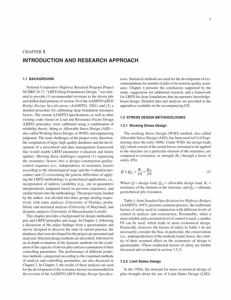
National Cooperative Highway Research Program ProjectNCHRP 24-17, “LRFD Deep Foundations Design,” was initi-ated to provide (1) recommended revisions to the driven pileand drilled shaft portions of section 10 of the AASHTO LRFDBridge Design Specifications (AASHTO, 2001) and (2) adetailed procedure for calibrating deep foundation resistancefactors. The current AASHTO specifications, as well as otherexisting codes based on Load and Resistance Factor Design(LRFD) principles, were calibrated using a combination ofreliability theory, fitting to Allowable Stress Design (ASD—also called Working Stress Design, or WSD), and engineeringjudgment. The main challenges of the project were, therefore,the compilation of large, high-quality databases and the devel-opment of a procedural and data management frameworkthat would enable LRFD parameter evaluation and futureupdates. Meeting these challenges required (1) organizingthe resistance factors into a design-construction-quality-control sequence (i.e., independence in resistance factorsaccording to the chronological stage and the evaluation pro-cedure) and (2) overcoming the generic difficulties of apply-ing the LRFD methodology to geotechnical applications, i.e.,incorporation of indirect variability (e.g., site or parametersinterpretation), judgment based on previous experience, andsimilar factors into the methodology. The project team, headedby the author, was divided into three groups dealing respec-tively with static analyses (University of Florida), proba-bilistic and structural analyses (University of Maryland), anddynamic analyses (University of Massachusetts Lowell).
This chapter provides a background for design methodolo-gies and LRFD principles and usage. In Chapter 2, followinga discussion of the major findings from a questionnaire andsurvey designed to discover the state of current practice, thedatabases that were developed for the project are presented andanalyzed. Selected design methods are described, followed byan in-depth evaluation of the dynamic methods for the evalu-ation of the capacity of driven piles and an examination of theircontrolling parameters. The performance of different predic-tion methods, categorized according to the examined methodsof analysis and controlling parameters, are also discussed inChapter 2. In Chapter 3, the results of these analyses are usedfor the development of the resistance factors recommended forthe revision of the AASHTO LRFD Bridge Design Specifica-
tions. Statistical methods are used for the development of rec-ommendations for number of piles to be tested in quality assur-ance. Chapter 4 presents the conclusions supported by thestudy, suggestions for additional research, and a frameworkfor LRFD for deep foundations that incorporates knowledge-based design. Detailed data and analyses are provided in theappendices available on the accompanying CD.
1.2 STRESS DESIGN METHODOLOGIES
1.2.1 Working Stress Design
The working Stress Design (WSD) method, also calledAllowable Stress Design (ASD), has been used in Civil Engi-neering since the early 1800s. Under WSD, the design loads(Q), which consist of the actual forces estimated to be appliedto the structure (or a particular element of the structure), arecompared to resistance, or strength (Rn ) through a factor ofsafety (FS):
(1)
Where Q = design load; Qall = allowable design load; Rn =resistance of the element or the structure, and Qult = ultimategeotechnical pile resistance.
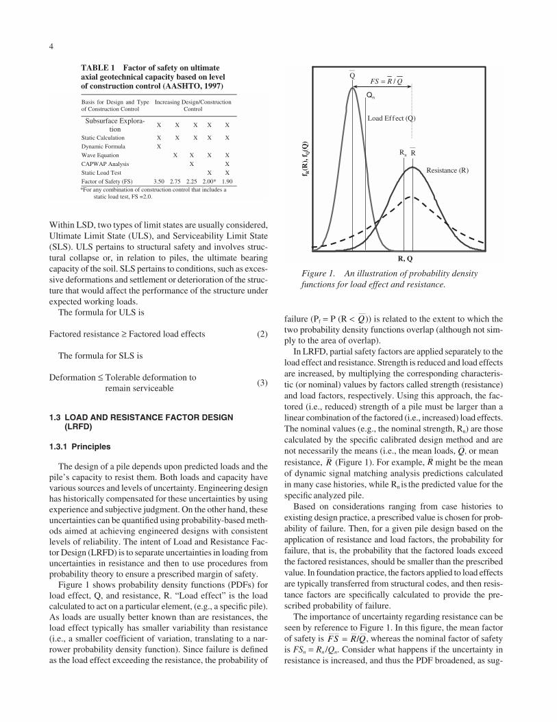
Table 1, from Standard Specifications for Highway Bridges(AASHTO, 1997), presents common practice, the traditionalfactors of safety used in conjunction with different levels ofcontrol in analysis and construction. Presumably, when amore reliable and consistent level of control is used, a smallerFS can be used, which leads to more economical design.Practically, however, the factors of safety in Table 1 do notnecessarily consider the bias, in particular, the conservatism(i.e., underprediction) of the methods listed; hence, the valid-ity of their assumed effect on the economics of design isquestionable. (These traditional factors of safety are furtherdiscussed and evaluated in section 3.5.2)
1.2.2 Limit States Design
In the 1950s, the demand for more economical design ofpiles brought about the use of Limit States Design (LSD).
Q QRFS
QFSall
n ult≤ = =
Within LSD, two types of limit states are usually considered,Ultimate Limit State (ULS), and Serviceability Limit State(SLS). ULS pertains to structural safety and involves struc-tural collapse or, in relation to piles, the ultimate bearingcapacity of the soil. SLS pertains to conditions, such as exces-sive deformations and settlement or deterioration of the struc-ture that would affect the performance of the structure underexpected working loads.
The formula for ULS is
Factored resistance ≥ Factored load effects (2)
The formula for SLS is
Deformation ≤ Tolerable deformation to remain serviceable
(3)
1.3 LOAD AND RESISTANCE FACTOR DESIGN(LRFD)
1.3.1 Principles
The design of a pile depends upon predicted loads and thepile’s capacity to resist them. Both loads and capacity havevarious sources and levels of uncertainty. Engineering designhas historically compensated for these uncertainties by usingexperience and subjective judgment. On the other hand, theseuncertainties can be quantified using probability-based meth-ods aimed at achieving engineered designs with consistentlevels of reliability. The intent of Load and Resistance Fac-tor Design (LRFD) is to separate uncertainties in loading fromuncertainties in resistance and then to use procedures fromprobability theory to ensure a prescribed margin of safety.
Figure 1 shows probability density functions (PDFs) forload effect, Q, and resistance, R. “Load effect” is the loadcalculated to act on a particular element, (e.g., a specific pile).As loads are usually better known than are resistances, theload effect typically has smaller variability than resistance(i.e., a smaller coefficient of variation, translating to a nar-rower probability density function). Since failure is definedas the load effect exceeding the resistance, the probability of
4
failure (Pf = P (R < )) is related to the extent to which thetwo probability density functions overlap (although not sim-ply to the area of overlap).
In LRFD, partial safety factors are applied separately to theload effect and resistance. Strength is reduced and load effectsare increased, by multiplying the corresponding characteris-tic (or nominal) values by factors called strength (resistance)and load factors, respectively. Using this approach, the fac-tored (i.e., reduced) strength of a pile must be larger than alinear combination of the factored (i.e., increased) load effects.The nominal values (e.g., the nominal strength, Rn) are thosecalculated by the specific calibrated design method and arenot necessarily the means (i.e., the mean loads, , or meanresistance, (Figure 1). For example, might be the meanof dynamic signal matching analysis predictions calculatedin many case histories, while Rn is the predicted value for thespecific analyzed pile.
Based on considerations ranging from case histories toexisting design practice, a prescribed value is chosen for prob-ability of failure. Then, for a given pile design based on theapplication of resistance and load factors, the probability forfailure, that is, the probability that the factored loads exceedthe factored resistances, should be smaller than the prescribedvalue. In foundation practice, the factors applied to load effectsare typically transferred from structural codes, and then resis-tance factors are specifically calculated to provide the pre-scribed probability of failure.
The importance of uncertainty regarding resistance can beseen by reference to Figure 1. In this figure, the mean factorof safety is , whereas the nominal factor of safetyis FSn = Rn /Qn. Consider what happens if the uncertainty inresistance is increased, and thus the PDF broadened, as sug-
FS R Q= /
RRQ
Q
Basis for Design and Type of Construction Control
Increasing Design/Construction Control
Subsurface Explora-tion
X X X X X
Static Calculation X X X X X
Dynamic Formula X
Wave Equation X X X X
CAPWAP Analysis X X
Static Load Test X X
Factor of Safety (FS) 3.50 2.75 2.25 2.00* 1.90 *For any combination of construction control that includes a
static load test, FS =2.0.
TABLE 1 Factor of safety on ultimateaxial geotechnical capacity based on level of construction control (AASHTO, 1997)
R, Q
f R(R
), f Q
(Q)
Load Effect (Q)
Resistance (R)
__Q
__RRn
Qn
QRFS /=
Figure 1. An illustration of probability densityfunctions for load effect and resistance.
gested by the dashed curve. The mean resistance for thisother predictive method remains unchanged, but the varia-tion (i.e., uncertainty) is increased.
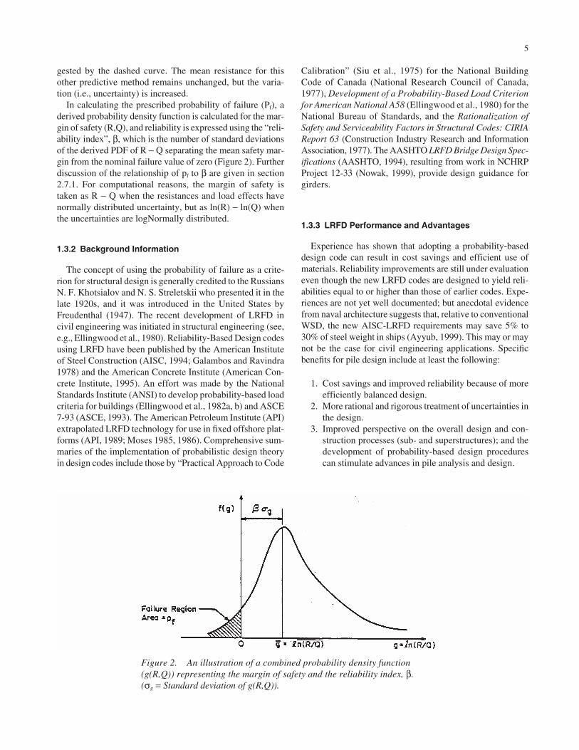
In calculating the prescribed probability of failure (Pf), aderived probability density function is calculated for the mar-gin of safety (R,Q), and reliability is expressed using the “reli-ability index”, β, which is the number of standard deviationsof the derived PDF of R − Q separating the mean safety mar-gin from the nominal failure value of zero (Figure 2). Furtherdiscussion of the relationship of pf to β are given in section2.7.1. For computational reasons, the margin of safety istaken as R − Q when the resistances and load effects havenormally distributed uncertainty, but as ln(R) − ln(Q) whenthe uncertainties are logNormally distributed.
1.3.2 Background Information
The concept of using the probability of failure as a crite-rion for structural design is generally credited to the RussiansN. F. Khotsialov and N. S. Streletskii who presented it in thelate 1920s, and it was introduced in the United States byFreudenthal (1947). The recent development of LRFD incivil engineering was initiated in structural engineering (see,e.g., Ellingwood et al., 1980). Reliability-Based Design codesusing LRFD have been published by the American Instituteof Steel Construction (AISC, 1994; Galambos and Ravindra1978) and the American Concrete Institute (American Con-crete Institute, 1995). An effort was made by the NationalStandards Institute (ANSI) to develop probability-based loadcriteria for buildings (Ellingwood et al., 1982a, b) and ASCE7-93 (ASCE, 1993). The American Petroleum Institute (API)extrapolated LRFD technology for use in fixed offshore plat-forms (API, 1989; Moses 1985, 1986). Comprehensive sum-maries of the implementation of probabilistic design theoryin design codes include those by “Practical Approach to Code
5
Calibration” (Siu et al., 1975) for the National BuildingCode of Canada (National Research Council of Canada,1977), Development of a Probability-Based Load Criterionfor American National A58 (Ellingwood et al., 1980) for theNational Bureau of Standards, and the Rationalization ofSafety and Serviceability Factors in Structural Codes: CIRIAReport 63 (Construction Industry Research and InformationAssociation, 1977). The AASHTO LRFD Bridge Design Spec-ifications (AASHTO, 1994), resulting from work in NCHRPProject 12-33 (Nowak, 1999), provide design guidance forgirders.
1.3.3 LRFD Performance and Advantages
Experience has shown that adopting a probability-baseddesign code can result in cost savings and efficient use ofmaterials. Reliability improvements are still under evaluationeven though the new LRFD codes are designed to yield reli-abilities equal to or higher than those of earlier codes. Expe-riences are not yet well documented; but anecdotal evidencefrom naval architecture suggests that, relative to conventionalWSD, the new AISC-LRFD requirements may save 5% to30% of steel weight in ships (Ayyub, 1999). This may or maynot be the case for civil engineering applications. Specificbenefits for pile design include at least the following:
1. Cost savings and improved reliability because of moreefficiently balanced design.
2. More rational and rigorous treatment of uncertainties inthe design.
3. Improved perspective on the overall design and con-struction processes (sub- and superstructures); and thedevelopment of probability-based design procedurescan stimulate advances in pile analysis and design.
Figure 2. An illustration of a combined probability density function(g(R,Q)) representing the margin of safety and the reliability index, β. (σg = Standard deviation of g(R,Q)).
4. Transformation of the codes into living documents thatcan be easily revised to include new information reflect-ing statistical data on design factors.
5. The partial safety factor format used herein also pro-vides a framework for extrapolating existing designpractice to new foundation concepts and materials whereexperience is limited.
1.3.4 LRFD in Geotechnical Engineering
Early use of LSD for geotechnical applications was exam-ined by the Danish geotechnical institute (Hansen 1953, 1956)and later formulated into code (Hansen, 1966). Independentload and resistance factors were used, with the resistance fac-tors applied directly to the soil properties rather than to thenominal resistance.
Considerable effort has been directed over the past decadeon the application of LRFD in geotechnical engineering.LRFD approaches have been developed in offshore engi-neering (e.g., Tang, 1993; Hamilton and Murff, 1992), gen-eral foundation design (e.g., Kulhawy et al., 1996), and piledesign for transportation structures (Barker et al., 1991;O’Neill, 1995).
In geotechnical practice, uncertainties concerning resis-tance principally manifest themselves in design methodology,site characterization, soil behavior, and construction quality.The uncertainties have to do with the formulation of the phys-ical problem, interpreting site conditions, understanding soilbehavior (e.g., its representation in property values), andaccounting for construction effects. Uncertainties in externalloads are small compared with uncertainties in soil and waterloads and the strength-deformation behaviors of soils. Theapplied loads, however, are traditionally based on superstruc-ture analysis, whereas actual load transfer to substructures ispoorly researched. The approach for selecting load and resis-tance factors developed in structural practice, though a usefulstarting point for geotechnical applications, is not sufficient.Work is needed to incorporate factors that are unique to geo-technical design into the LRFD formulation.
Philosophically, the selection of load and resistance factorsdoes not have to be made probabilistically, although in currentstructural practice a calibration based on reliability theory iscommonly used. This approach focuses more on load uncer-tainties than resistance uncertainties and does not includemany subjective factors unique to geotechnical practice. Anexpanded approach is needed if the full benefits of LRFD areto be achieved for foundation design. The National ResearchCouncil reports that the “subjective approach reflects the gen-eral lack of robust data sources from which a more objectiveset of factors can be derived” (National Research Council,1995). The report continues, “realistically, because of thetremendous range of property values and site conditions thatone may encounter, it is unlikely that completely objectivefactors can be developed in the foreseeable future.”
6
Today, the situation has changed somewhat, but notentirely. The present research team gathered robust data onpile capacity from which a more objective calibration of resis-tance factors could be made. Nonetheless, there remain uncer-tainties associated with (1) site conditions, (2) soil behaviorand the interpretation of soil parameters, and (3) constructionmethods and quality. These factors are difficult to understandfrom the pile databases alone. Such knowledge-based factorsshould be combined with the reliability-theory-based cali-bration of the database records to achieve a meaningful LRFDapproach, requiring a major research effort. These difficul-ties are addressed in the present research through the cali-bration of specific combinations of design and parameterinterpretation methods.
1.3.5 LRFD for Deep Foundations
Several efforts have been made to develop LRFD-basedcodes for deep foundation design.
1.3.5.1 2001 AASHTO LRFD Bridge DesignSpecifications for Driven Piles
LRFD Bridge Design Specifications (AASHTO, 2001)states that the ultimate resistance (Rn) multiplied by a resis-tance factor (φ), which thus becomes the factored resistance(Rr), must be greater than or equal to the summation of loads(Qi) multiplied by corresponding load factors (γi), and amodifier (ηi). For strength limit states:
(4)
where:
ηi = ηDηRηI > 0.95 (5)
where ηi = factors to account for; ηD = effects of ductility;ηR = redundancy; and ηI = operational importance.
The Specifications provide the following equations fordetermining the factored bearing resistance of piles, QR,
QR = φQn = φqQult = φqpQp + φqsQs (6)
for which:
Qp = qp Ap (7)
Qs = qs As (8)
where φq = resistance factor for the bearing resistance of a sin-gle pile specified for methods that do not distinguish betweentotal resistance and the individual contributions of tip resis-tance and shaft resistance; Qult = bearing resistance of a single
R R Qr n i i i= ≥ ∑φ η γ
pile; Qp = pile tip resistance; Qs = pile shaft resistance (F);qp = unit tip resistance of pile; qs = unit shaft resistance ofpile; As = surface area of pile shaft; Ap = area of pile tip; andφqp, φqs = resistance factor for tip and shaft resistance, respec-tively, for those methods that separate the resistance of a pileinto contributions from tip resistance and shaft resistance.
The resistance factors for use in the above equations are pre-sented in Table 10.5.5-2 of the Specifications for differentdesign methods based on soil type and area of resistance (tipand side). The resistance factors for compression vary between0.45 and 0.70. The table also incorporates a factor, λv, for dif-ferent methods and level of field capacity verification. As anexample, if, in analysis, an α method is used to determine thepile’s friction resistance in clay, a resistance factor of 0.70 isrecommended. If, in verification of the pile capacity, a piledriving formula, e.g., an ENR (Engineering News-Record)equation, is used without stress wave measurements duringdriving, a λv factor of 0.80 is recommended. The actual resis-tance factor to be used in the above analysis verificationsequence is, therefore, 0.56 (i.e., 0.70 × 0.80).
1.3.5.2 2001 AASHTO LRFD Bridge DesignSpecifications for Drilled Shafts
LRFD Bridge Design Specifications (AASHTO, 2001)provides detailed resistance factors for a large number ofdesign methods for drilled shafts. Differentiation is madebetween base and side resistance, as for driven piles, withresistance factors varying between 0.45 and 0.65. Static test-ing is included with the same resistance factor as for drivenpiles (0.8). Resistance factors are not provided for drilledshafts in sand. The λv factor, used for field verification fordriven piles, is not used for drilled shafts, and no distinctionis made on the basis of construction method.
1.3.5.3 Worldwide LRFD Codes for DeepFoundations and Drilled Shafts
A review of foundation design standards in the world wasconducted by the Japanese Geotechnical Society (1998). Areview of the development of LRFD applications for Geo-technical Engineering is presented by Goble (1999). A reviewof LRFD parameters for dynamic analyses of piles is pre-sented by Paikowsky and Stenerson in Appendix B. Thepresent section provides a short review of non-US LRFDcodes for deep foundations.
The Australian Standard for Piling-Design and Installa-tion (1995) provides ranges of resistance factors for staticload tests (0.7 to 0.9) and static pile analyses (0.40–0.65)related to the source of soil parameters and soil type (e.g.,SPT in cohesionless soils). Detailed recommendations areprovided for resistance factors to be used with the dynamicmethods ranging between 0.45 to 0.65 for methods withoutdynamic measurements (including WEAP), and between
7
0.50 to 0.85 when utilizing dynamic measurements with sig-nal matching analysis. Selection of the appropriate resis-tance factor depends on driving conditions, geotechnicalfactors (e.g., extent of site investigation), and extent of test-ing (e.g., low range for <3% of the pile tested and high rangefor >15%). In traditional structural design specifications, anominal value is given and the value used is based primar-ily on engineering judgment and cannot exceed the nominalvalue. The Australian Standard is therefore unique by pro-viding a guide for choosing the appropriate resistance fac-tor. Interestingly, no distinction is made regarding either soiltype or time of driving (i.e. EOD, BOR) when referring tothe signal matching based on dynamic measurements. Themethod by which the resistance factors were generated is notprovided in the code.
The AUSTROADS Bridge Design Code (1992) providesresistance factors for the construction stage alone includingstatic load test (to failure φ = 0.9, proof test φ = 0.8), and fourcategories of dynamic methods. The range of resistance fac-tors is quite large and there is no explanation as to how theresistance factors were obtained. Goble (1999) postulates thatthe resistance factors were calibrated via the working stressdesign method.
The Ontario Bridge Code (1992) recommends relativelylow resistance factors with no differentiation between theindividual static or dynamic analyses. For example, the resis-tance factors for static analyses and static load tests in com-pression and tension are 0.4, 0.3, 0.6 and 0.4 respectively. Noinformation is provided on how the resistance factors wereobtained.
The Bridge Code (1992) is brief in its design requirementsfor deep foundations. Resistance factors are based on piletype, φ = 0.4 for all timber and concrete piles (precast, filledpipe, and cast in place) and 0.5 for steel piles. For dynamicload testing, resistance factors of 0.4 and 0.5 are recom-mended for routine testing and analyses based on dynamicmeasurements, respectively.
Eurocode 7 (1997) deals with driven piles and drilledshafts at a single section. Factors for static load testingdepend on the number of tested piles (irrelevant to the num-ber of piles at the specific site). Range of values from 0.67 to0.91 is provided for one to three tests, related to the mean orlowest value of the test results. The code is quite complexwith quantitative descriptions and limiting conditions. Thecode is presented with multiple component factors, and forcomparison with the form used by U.S. codes, Goble (1999)inverted and combined the factors resulting in values rang-ing from 0.63 to 0.77 for base, skin, and total resistance ofdriven, bored, and CFA piles. DiMaggio et al. (1998) pre-sented a summary report of a geotechnical engineering studytour, stating “The team found Eurocode 7 to be a difficult doc-ument to read and understand, which may explain the variousinterpretations that were expressed in the countries visited.”Improvements in that direction were achieved through a text

that explains the methodology and provides design examples(Orr and Farrell, 1999; see also Orr, 2002). The final draft ofthe future Eurocode 7 (October 2001, see also Frank, 2002)is an extensive code that is expected to become an EN pub-lication by August 2004. This detailed document contains12 sections dealing with all geotechnical design aspects rang-ing from geotechnical data (section 3), to construction super-vision (section 4), to hydraulic failure (section 10). Section 7is dedicated to pile foundations. While not very detailedregarding a specific determination of the pile capacity, thecode is elaborating for all cases (i.e., static load test results,static and dynamic methods) factors to be applied to both theminimum and average of the capacity as a function of thenumber of applications. For example, static load test capac-ity will have factors (to be divided by) ranging from 1.4 to1.0 when applied to the results of 1 to 5 or over load tests.Specifically, if, for example, three static load tests are carriedout, the mean value of the three will be divided by 1.2, andthe minimum value by 1.05, and the lower of the two willdetermine the factored resistance to be used.
Substantially fewer details are provided by the codes forLRFD design of drilled shafts. The two extremes being theaforementioned Bridge Code (1992), in which drilled shaftsare included under a single category of cast-in-place piles(φ = 0.4 like all other concrete piles), and the AASHTO rel-atively detailed provisions described in section 1.3.5.2.
1.3.5.4 Difficulties with the Existing LRFD Codes
All existing codes suffer from two major difficulties.One is the application of LRFD to geotechnical problemsas described in section 1.3.4 (e.g., site variability, con-struction effects, past experience, etc.). The other problemis lack of data. None of the reviewed codes and associatedresistance factors were consistently developed based on data-bases enabling the calculation of resistance factors from casehistories.
The current AASHTO specifications of driven pilesreviewed in section 1.3.5.1 encounter additional difficultydue to the multiplication of the resistance factor by the mod-ifier λv. This procedure requires the interaction of two inde-pendent pile capacity evaluations (e.g., static analysis anddynamic methods) and results in unnecessary and confusingconservatism. A clear separation of the resistance factors onthe basis of design and construction is required and is oneaim of the present study. As a result of the aforementioneddifficulties, the current AASHTO LRFD specifications forgeotechnical applications are of limited use. Two surveyspresented in this report (see section 2.1) found that only14 states (30%) are currently committed to the use of LRFDin foundation design. In contrast 93% of the responding useWSD, suggesting that most of those that use LRFD are uti-lizing the methodology in parallel to WSD.
8
1.4 RESEARCH APPROACH
1.4.1 Design and Construction Process of Deep Foundations
Figure 3 presents a flow chart depicting the design andconstruction process of deep foundations. Commonly, designstarts with site investigation and soil parameter evaluation,assessments that vary in quality and quantity according to theimportance of the project and complexity of the subsurface.Possible foundation schemes are identified based on the resultsof the investigation, load requirements, and local practice. Allpossible schemes are evaluated via static analyses. Schemesfor driven piles also require dynamic analysis (drivability) forhammer evaluation, feasibility of installation, and structuraladequacy of the pile. In sum, the design stage combines,therefore, structural and geotechnical analyses to determinethe best prebidding design. This process leads to estimatedquantities to appear in construction bidding documents.
Upon construction initiation, static load testing and/ordynamic testing, or dynamic analysis based on driving resis-tance (using dynamic formulas or wave-equations) arecarried out on selected elements (i.e., indicator piles) of theoriginal design. Pile capacity is evaluated based on the con-struction phase testing results, which determine the assignedcapacity and final design specifications. In large or importantprojects, the pile testing may also be used as part of thedesign. Two requirements are evident from this process:(1) pile evaluation is carried out at both the design and theconstruction stage, and (2) these two evaluations shouldresult in foundation elements of the same reliability but pos-sibly different number and length of elements depending onthe information available at each stage.
1.4.2 Overview of the Research Approach
The complete application of LRFD to the process describedin Figure 3 requires an integrated framework. For example,the method by which a field test (say SPT) is used to obtainsoil parameters must be coordinated with the method used forstatic capacity of the pile, and both must be coordinated withthe assessment of uncertainty. Independently, one needs toevaluate the design verification process during construction,i.e., static load testing and dynamic testing to assess and mod-ify the pile installation, as well as quality assurance (e.g.,nondestructive testing of drilled shafts) and related issues.
Previous LRFD developments, using back analysis ofASD and judgment, have addressed some of these issues(e.g., Withiam et al., 1998). The present effort to assemble acase history database adds other difficulties, for exampledetermining a “predicted” capacity that can be comparedwith measured load-test values.
The present effort was focused on calibrating the directdesign and construction evaluation process. For the design,specific methods and correlations were chosen. Their results
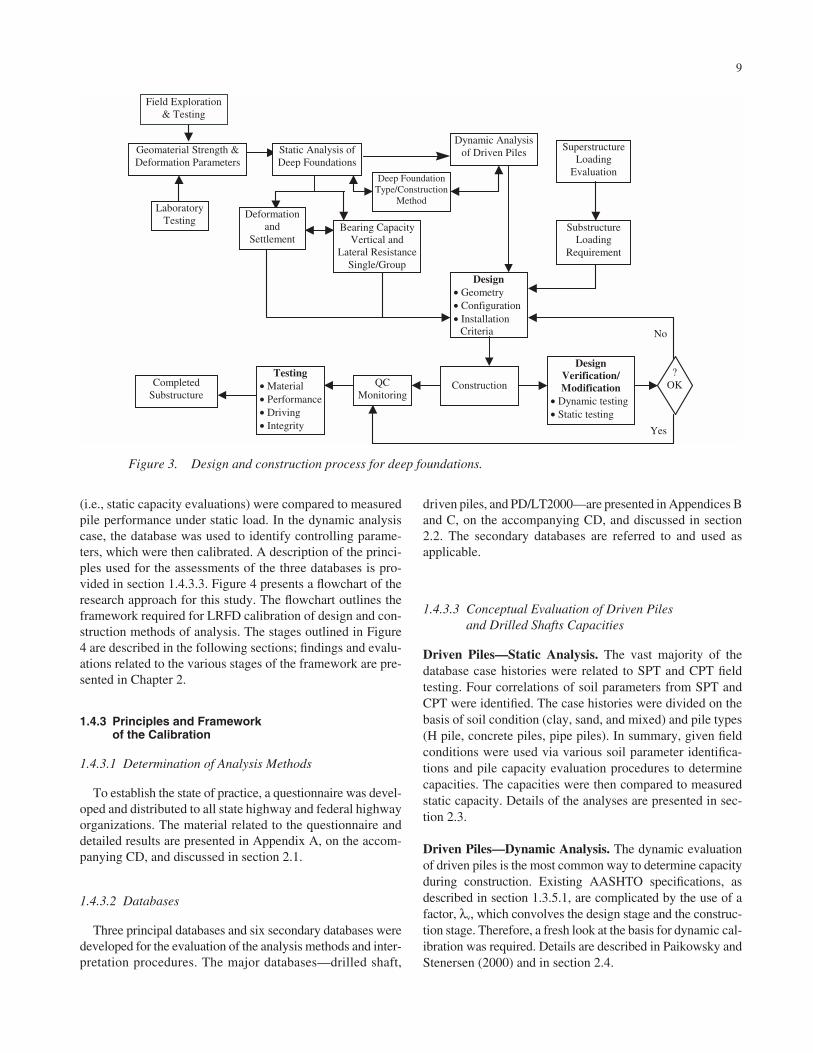
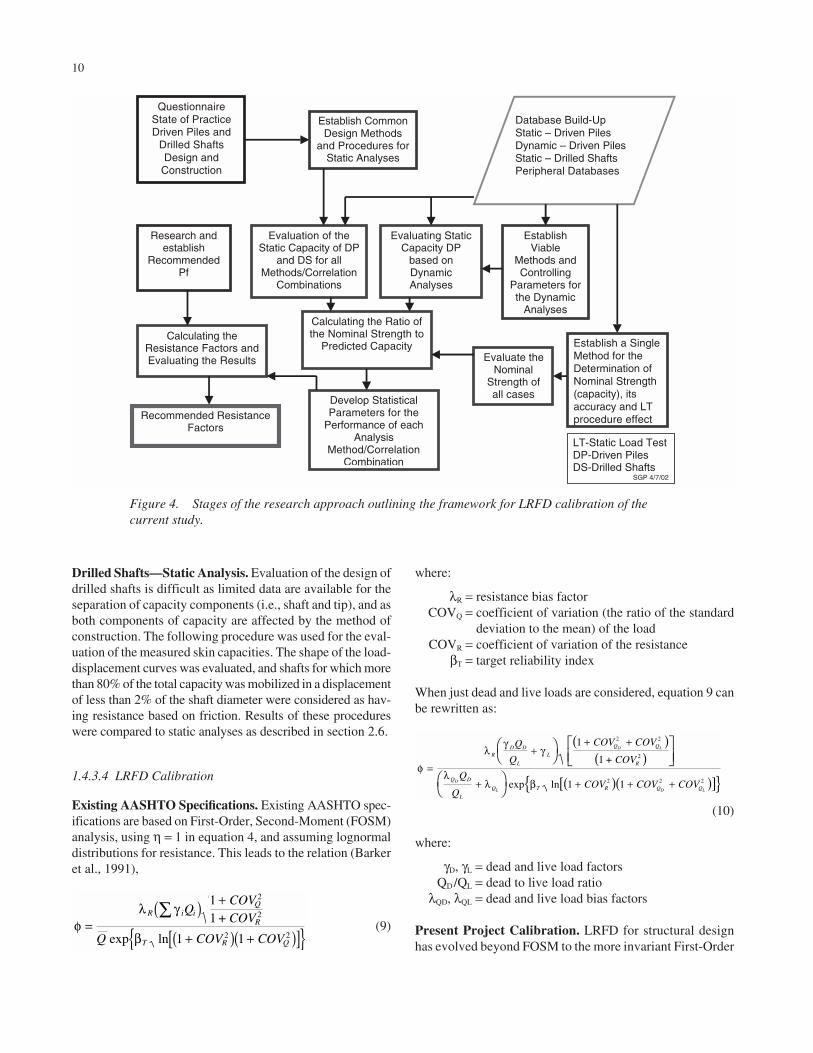
(i.e., static capacity evaluations) were compared to measuredpile performance under static load. In the dynamic analysiscase, the database was used to identify controlling parame-ters, which were then calibrated. A description of the princi-ples used for the assessments of the three databases is pro-vided in section 1.4.3.3. Figure 4 presents a flowchart of theresearch approach for this study. The flowchart outlines theframework required for LRFD calibration of design and con-struction methods of analysis. The stages outlined in Figure4 are described in the following sections; findings and evalu-ations related to the various stages of the framework are pre-sented in Chapter 2.
1.4.3 Principles and Framework of the Calibration
1.4.3.1 Determination of Analysis Methods
To establish the state of practice, a questionnaire was devel-oped and distributed to all state highway and federal highwayorganizations. The material related to the questionnaire anddetailed results are presented in Appendix A, on the accom-panying CD, and discussed in section 2.1.
1.4.3.2 Databases
Three principal databases and six secondary databases weredeveloped for the evaluation of the analysis methods and inter-pretation procedures. The major databases—drilled shaft,
9
driven piles, and PD/LT2000—are presented in Appendices Band C, on the accompanying CD, and discussed in section2.2. The secondary databases are referred to and used asapplicable.
1.4.3.3 Conceptual Evaluation of Driven Pilesand Drilled Shafts Capacities
Driven Piles—Static Analysis. The vast majority of thedatabase case histories were related to SPT and CPT fieldtesting. Four correlations of soil parameters from SPT andCPT were identified. The case histories were divided on thebasis of soil condition (clay, sand, and mixed) and pile types(H pile, concrete piles, pipe piles). In summary, given fieldconditions were used via various soil parameter identifica-tions and pile capacity evaluation procedures to determinecapacities. The capacities were then compared to measuredstatic capacity. Details of the analyses are presented in sec-tion 2.3.
Driven Piles—Dynamic Analysis. The dynamic evaluationof driven piles is the most common way to determine capacityduring construction. Existing AASHTO specifications, asdescribed in section 1.3.5.1, are complicated by the use of afactor, λv, which convolves the design stage and the construc-tion stage. Therefore, a fresh look at the basis for dynamic cal-ibration was required. Details are described in Paikowsky andStenersen (2000) and in section 2.4.
Yes
Geomaterial Strength & Deformation Parameters
Static Analysis of Deep Foundations
Laboratory Testing
Deformation and
Settlement Bearing Capacity
Vertical and Lateral Resistance
Single/Group
Deep Foundation Type/Construction
Method
Dynamic Analysis of Driven Piles
Design • Geometry • Configuration • Installation
Criteria
Superstructure Loading
Evaluation
Substructure Loading
Requirement
Completed Substructure
Testing • Material • Performance • Driving • Integrity
QC Monitoring
Construction
Design Verification/ Modification
• Dynamic testing • Static testing
? OK
No
Field Exploration & Testing
Figure 3. Design and construction process for deep foundations.
Drilled Shafts—Static Analysis. Evaluation of the design ofdrilled shafts is difficult as limited data are available for theseparation of capacity components (i.e., shaft and tip), and asboth components of capacity are affected by the method ofconstruction. The following procedure was used for the eval-uation of the measured skin capacities. The shape of the load-displacement curves was evaluated, and shafts for which morethan 80% of the total capacity was mobilized in a displacementof less than 2% of the shaft diameter were considered as hav-ing resistance based on friction. Results of these procedureswere compared to static analyses as described in section 2.6.
1.4.3.4 LRFD Calibration
Existing AASHTO Specifications. Existing AASHTO spec-ifications are based on First-Order, Second-Moment (FOSM)analysis, using η = 1 in equation 4, and assuming lognormaldistributions for resistance. This leads to the relation (Barkeret al., 1991),
(9)φλ γ
β=
( ) +
+( ) +( )[ ]{ }∑R i i
Q
R
T R Q
QCOVCOV
Q COV COV
1
1 1
2
2
2 2
1 +
exp ln
10
where:
λR = resistance bias factorCOVQ = coefficient of variation (the ratio of the standard
deviation to the mean) of the loadCOVR = coefficient of variation of the resistance
βT = target reliability index
When just dead and live loads are considered, equation 9 canbe rewritten as:
(10)
where:
γD, γL = dead and live load factorsQD/QL = dead to live load ratio
λQD, λQL = dead and live load bias factors
Present Project Calibration. LRFD for structural designhas evolved beyond FOSM to the more invariant First-Order
φ
λγ
γ
λλ β
=
++ +
+ + + +
( )( )
( )( )[ ]{ }
RD D
L
L
Q Q
R
Q D
L
Q T R Q Q
Q
Q
COV COV
COV
Q
QCOV COV COV
D L
D
L D L
1
1 1
2 2
2
2 2 2
1 +
exp ln
Database Build-Up Static – Driven Piles Dynamic – Driven Piles Static – Drilled Shafts Peripheral Databases
QuestionnaireEstablish CommonDesign Methods
and Procedures forStatic Analyses
Research andestablish
RecommendedPf
Evaluation of theStatic Capacity of DP
and DS for allMethods/Correlation
Combinations
Evaluating StaticCapacity DP
based onDynamicAnalyses
EstablishViable
Methods andControlling
Parameters forthe Dynamic
Analyses
Establish a Single Method for the Determination of Nominal Strength (capacity), its accuracy and LT procedure effect
Calculating the Ratio ofthe Nominal Strength to
Predicted Capacity
LT-Static Load Test DP-Driven Piles DS-Drilled Shafts
SGP 4/7/02
Evaluate theNominal
Strength ofall casesDevelop Statistical
Parameters for thePerformance of each
AnalysisMethod/Correlation
Combination
Calculating theResistance Factors andEvaluating the Results
Recommended ResistanceFactors
State of PracticeDriven Piles and
Drilled ShaftsDesign and
Construction
Figure 4. Stages of the research approach outlining the framework for LRFD calibration of thecurrent study.
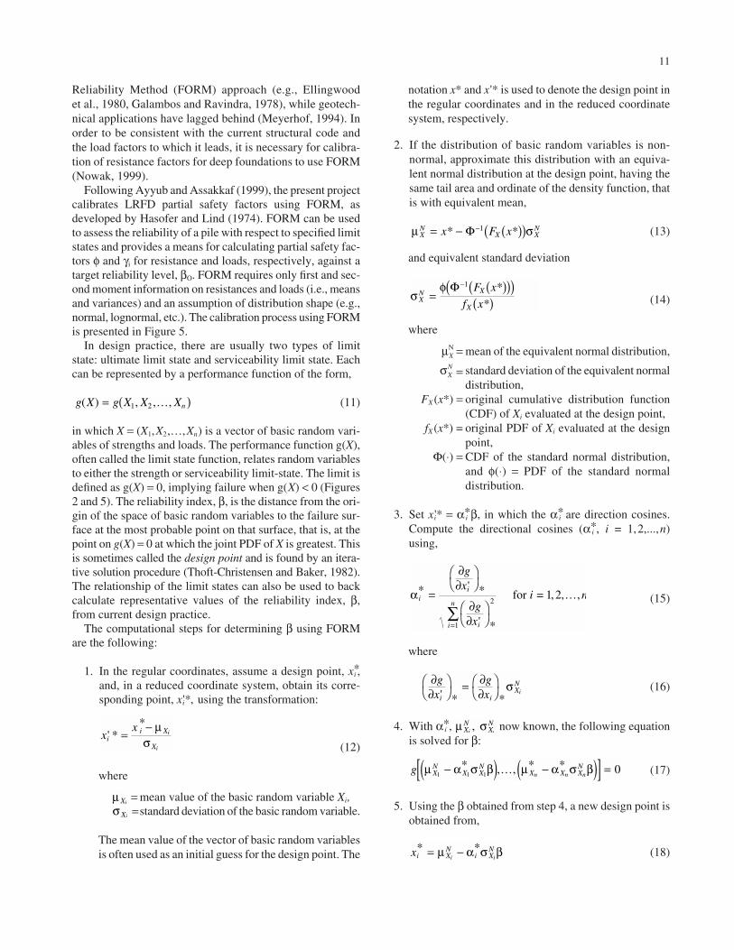
Reliability Method (FORM) approach (e.g., Ellingwood et al., 1980, Galambos and Ravindra, 1978), while geotech-nical applications have lagged behind (Meyerhof, 1994). Inorder to be consistent with the current structural code andthe load factors to which it leads, it is necessary for calibra-tion of resistance factors for deep foundations to use FORM(Nowak, 1999).
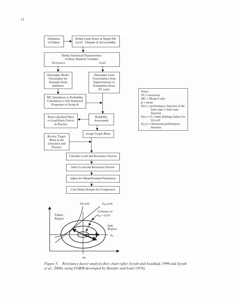
Following Ayyub and Assakkaf (1999), the present projectcalibrates LRFD partial safety factors using FORM, asdeveloped by Hasofer and Lind (1974). FORM can be usedto assess the reliability of a pile with respect to specified limitstates and provides a means for calculating partial safety fac-tors φ and γi for resistance and loads, respectively, against atarget reliability level, βO. FORM requires only first and sec-ond moment information on resistances and loads (i.e., meansand variances) and an assumption of distribution shape (e.g.,normal, lognormal, etc.). The calibration process using FORMis presented in Figure 5.
In design practice, there are usually two types of limitstate: ultimate limit state and serviceability limit state. Eachcan be represented by a performance function of the form,
(11)
in which X = (X1,X2,…,Xn) is a vector of basic random vari-ables of strengths and loads. The performance function g(X),often called the limit state function, relates random variablesto either the strength or serviceability limit-state. The limit isdefined as g(X) = 0, implying failure when g(X) < 0 (Figures2 and 5). The reliability index, β, is the distance from the ori-gin of the space of basic random variables to the failure sur-face at the most probable point on that surface, that is, at thepoint on g(X) = 0 at which the joint PDF of X is greatest. Thisis sometimes called the design point and is found by an itera-tive solution procedure (Thoft-Christensen and Baker, 1982).The relationship of the limit states can also be used to backcalculate representative values of the reliability index, β,from current design practice.
The computational steps for determining β using FORMare the following:
1. In the regular coordinates, assume a design point, x*i ,
and, in a reduced coordinate system, obtain its corre-sponding point, x'*i , using the transformation:
(12)
where
= mean value of the basic random variable Xi,=standard deviation of the basic random variable.
The mean value of the vector of basic random variablesis often used as an initial guess for the design point. The
σ Xi
µ Xi
xx
ii X
X
i
i
' **
=− µσ
g X g X X Xn( ) , , ,= ( )1 2 K
11
notation x* and x'* is used to denote the design point inthe regular coordinates and in the reduced coordinatesystem, respectively.
2. If the distribution of basic random variables is non-normal, approximate this distribution with an equiva-lent normal distribution at the design point, having thesame tail area and ordinate of the density function, thatis with equivalent mean,
(13)
and equivalent standard deviation
(14)
where
µNX = mean of the equivalent normal distribution,
σNX = standard deviation of the equivalent normal
distribution,FX (x*) = original cumulative distribution function
(CDF) of Xi evaluated at the design point, fX (x*) = original PDF of Xi evaluated at the design
point,Φ(⋅) = CDF of the standard normal distribution,
and φ(⋅) = PDF of the standard normal distribution.
3. Set x'*i = α*i β, in which the α*
i are direction cosines.Compute the directional cosines (α*
i , i = 1,2,...,n)using,
(15)
where
(16)
4. With α*i , now known, the following equation
is solved for β:
(17)
5. Using the β obtained from step 4, a new design point isobtained from,
(18)xi XN
i XN
i i* *= −µ α σ β
g XN
X XN
X X XN
n n nµ α σ β µ α σ β1 1 1 0−( ) −( )[ ] =* , , * *K
µ σXN
XN
i i,
∂∂
∂∂
σgx
gxi i
XN
i' * *
=
α
∂∂
∂∂
ii
ii
n
gx
gx
i n* ' *
' *
=
=
∑2
1
1 2for = , , ,K
σφ
XN X
X
F x
f x=
( )( )( )( )
−Φ 1 **
µ σXN
X XNx F x= − ( )( )−* *Φ 1
12
Definition of Failure
Define Limit States at Single Pile Level: Ultimate & Serviceability
Define Statistical Characteristics of Basic Random Variables
Resistance Load
Determine Model Uncertainty for Strength (from
database)
MC Simulation or Probability Calculation to Get Statistical
Properties of Scalar R
Reliability Assessment
Back-calculated Beta vs Load Ratio Curves
in Practice
Review Target Betas in the
Literature and Practice
µR
Safe Region
Failure Region
Contours of fRS = fX(x)
µS
G(x)=0 GL(x)=0
Assign Target Betas
Calculate Load and Resistance Factors
Select Load and Resistance Factors
Adjust for Mean/Nominal Parameters
Case Study Designs for Comparison
Determine Load Uncertainties from Superstructure to Foundation (from
ST code) Notes: ST = structural MC = Monte Carlo µ = mean G(x) = performance function of the
limit state = limit state function
G(x) = 0 = limit defining failure for G(x)<0
GL(x) = linearized performance function
Figure 5. Resistance factor analysis flow chart (after Ayyub and Assakkaf, 1999 and Ayyubet al., 2000), using FORM developed by Hasofer and Lind (1974).

6. Repeat steps 1 to 5 until convergence of β is achieved.This reliability index is the shortest distance to the failuresurface from the origin in the reduced coordinate space.
FORM can be used to estimate partial safety factors suchas those found in the design format. At the failure point(R*,L*1 − … − L*n ), the limit state is given by,
(19)
or, in a more general form by,
(20)
The mean value of the resistance and the design point can be used to compute the mean partial safety factors fordesign as,
(21)
(22)
In developing code provisions, it is necessary to followcurrent design practice to ensure consistent levels of reliabil-ity over different pile types. Calibrations of existing designcodes are needed to make the new design formats as simpleas possible and to put them in a form that is familiar todesigners. For a given reliability index β and probability dis-tributions for resistance and load effects, the partial safetyfactors determined by the FORM approach may differ withfailure mode. For this reason, calibration of the calculatedpartial safety factors (PSFs) is important in order to maintainthe same values for all loads at different failure modes. In thecase of geotechnical codes, the calibration of resistance fac-tors is performed for a set of load factors already specific inthe structural code (see following section). Thus, the loadfactors are fixed. In this case, the following algorithm is usedto determine resistance factors:
1. For a given value of the reliability index, β, probabilitydistributions and moments of the load variables, andthe coefficient of variation for the resistance, computemean resistance R using FORM.
γµi
i
L
L
i
=*
φµ
= R
R
*
g X g x x xn( ) *, *, , *= ( ) =1 2 0K
g R L Ln= − − − =* * *1 0K
13
2. With the mean value for R computed in step 1, the par-tial safety factor, φ, is revised as:
(23)
where µLi and µR are the mean values of the load andstrength variables, respectively, and γi, i = 1, 2,…, n, arethe given set of load factors.
Load Conditions and Load Factors. The actual load trans-ferred from the superstructure to the foundations is, by andlarge, unknown, with very little long-term research havingbeen focused on the subject. The load uncertainties are taken,therefore, as those used for the superstructure analysis.LRFD Bridge Design Specifications (AASHTO, 2000) pro-vide five load combinations for the standard strength limitstate (using dead, live, vehicular, and wind loads) and two forthe extreme limit states (using earthquake and collision loads).The use of a load combination that includes lateral loadingmay at times be the restrictive loading condition for deepfoundations design. Pile lateral capacity is usually controlledby service limit state, and as such, was excluded from thescope of the present study, which focuses on the axial capac-ity of single piles/drilled shafts. The load combination forstrength I was therefore applied in its primary form as shownin the following limit state:
Z = R − D − LL (24)
Where R = strength or resistance of pile, D = dead load andLL = vehicular live loads. The probabilistic characteristics ofthe random variables D and LL are assumed to be those usedby AASHTO (Nowak, 1999) with the following load factorsand lognormal distributions (bias and COV) for live and deadloads, respectively:
γL = 1.75 λQL = 1.15 COVQL = 0.2 (25)
γD = 1.25 λQD = 1.05 COVQD = 0.1 (26)
For the strength or resistance (R), the probabilistic charac-teristics are defined in Chapter 3, based on the databases forthe various methods and conditions that are described inChapter 2.
φγ µ
µ= =
∑ i Lii
n
R
1
14
CHAPTER 2
FINDINGS
2.1 STATE OF PRACTICE
2.1.1 Questionnaire and Survey
Code development requires examining the state of practicein design and construction in order to address the needs,research the performance, and examine alternatives. The iden-tification of current design and construction methodologieswas carried out via a questionnaire along with a survey, whichwas independently developed and analyzed by Mr. A. Munozof the FHWA. The questionnaire was distributed to 298 statehighway officials, TRB representatives, and state and FHWAgeotechnical engineers. A total of 45 surveys were returnedand analyzed (43 states and 2 FHWA personnel). The surveyelicited information concerning design methodology in geo-technical and structural design, foundation alternatives, anddesign and constitution considerations for both driven pilesand drilled shafts. The questionnaire, the survey, and theiranalyzed results are presented in Appendix A. A summaryanalysis of the survey results is presented below.
2.1.2 Major Findings
2.1.2.1 Design Methodology
Averaging the responses for driven piles and drilled shafts,about 90% of the respondents used ASD, 35% used AASHTOLoad Factor Design (LFD), and 28% used AASHTO Loadand Resistance Factors Design (LRFD), suggesting that mostof the respondents that use LRFD or LFD use it in parallelwith WSD.
Among the respondents using ASD to evaluate capacity,95% used a global safety factor ranging from 2.0 to 3.0,depending on construction control and 5% used partial safetyfactors of 1.5 to 2.0 for side friction (3.0 for drilled shafts)and 3.0 for end bearing (2.0 to 3.0 for drilled shafts).
2.1.2.2 Foundation Alternatives
The majority of the respondents use primarily driven pilefoundations (75%), 14% use shallow foundations, and 11%
use drilled shafts. Of those responding, 64% prefer the use ofdriven piles and 5% prefer drilled shafts or other foundationtype. When using driven piles, 21% primarily use prestressedconcrete piles; 52%, steel H piles; 2%, open-ended steel pipepiles; and 25%, closed-end steel pipe piles.
2.1.2.3 Driven Piles—Design Considerations
1. The most common methods used for evaluating the static axial capacity of driven piles were as follows:• 59%: α-method (Tomlinson, 1987),• 25%: β-method (Esrig & Kirby, 1979),• 5%: λ−method (Vijayvergiya and Focht, 1972),• 75%: Nordlund’s method (Nordlund, 1963),• 5%: Nottingham and Schmertmann’s method: CPT
(1975),• 9%: Schmertmann’s method: SPT (Sharp, 1987),• 14%: Meyerhof’s method (1976) modified by Zeitlen
and Paikowsky (1982), and• 25%: in-house methods and other less common
methods. Of the computer programs used in design,• 39% were developed in-house,• 75% were FHWA developed, and• 20% were from commercial vendors.
2. Of the primary tests used to assess strength parametersin design, 86% used SPT-N values, 11% used CPT data,2% used Dilatometer data, and none used Pressure-meter data.
3. The majority of the states used Tomlinson’s method toassess the side friction coefficient in cohesive soil (CA −adhesion) and Nordland’s method in cohesionless soil(δ − interfacial friction angle).
4. Pile settlement in the design was considered by 48%,with settlement ranging from 0.25 to 1.0 inches beingtolerable.
5. Simplified methods (e.g., Broms, 1964) were used by34% of the respondents in the lateral pile design meth-ods and/or computer programs, and 88% used methodsbased on p-y curves. Of the computer programs used indesign, 14% were in-house, 82% were from the FHWA,and 55% came from commercial vendors.
15
6. Responses for the estimated risk or failure probabilityof the group foundation design were as follows:• 27% less than 0.1%,• 4% between 0.1 and 1%,• 1% of the responses were between 1% and 10%, and• 67% were unknown.
The assessment for the acceptable maximum failure proba-bility ranged from about 0 to 1%. Pile failure had been expe-rienced by 14% of the respondents.
2.1.2.4 Driven Piles—ConstructionConsiderations
1. Of the respondents, 77% performed static pile load testduring construction, and the primary test method wasthe Quick Method.
2. The most common dynamic methods used for capacityevaluation of driven piles included the following: • Wave Equation Analysis using the program GRL-
WEAP (GRL Engineers, Inc. Wave Equation Analy-sis Program) was used by 80% of the respondents.
• 45% used the ENR formula,• 16% used Gate’s equation with safety factors rang-
ing from 2.0 to 3.5, and• 1 state used its own dynamic formula.
3. Dynamic pile load tests were performed during con-struction by 84 % of respondents, testing 1% to 10% ofthe piles per bridge.
4. When setting production pile length and driving crite-ria, 82% used EOD conditions, 52% used BOR condi-tions, and 36% did not consider pile freeze or relax-ation effects in determining driving criteria.
2.1.2.5 Drilled Shafts—Design Considerations
1. The most common methods used for evaluating thestatic axial capacity of drilled shafts were as follows:• 36%: the α-method (total stress approach) (Reese
and O’Neill, 1998; Kulhawy, 1989),• 41%: the β-method (effective stress approach) (Reese
and O’Neill, 1988),• 9%: the Reese and Wright (1977) approach for side
friction in cohesionless soils,• 39%: the FHWA (O’Neill et al., 1996) approach for
intermediate geomaterials (soft rock),• 11%: Carter and Kulhawy (1988) approach for inter-
mediate geomaterials (soft rock), and • 27%: other methods.
Of the computer programs used, 18% were developedin-house, 50% came from the FHWA, 29% from com-mercial vendors, and 20% from others.
2. Of the primary parameters used, 70% were based on SPTvalues, 7% were obtained from the CPT test, 2% werebased on Pressuremeter data, and 2% were based onDilatometer data.
3. Of the 16% considering the roughness of the boreholewall in rock socket design, all did so by assumption.
4. Shaft settlement was considered by 61% of the respon-dents, with tolerable settlements ranging from 0.25 to2.0 in.
5. Simplified (e.g., Brooms, 1964) lateral drilled shaftdesign methods and/or computer programs were usedby 27%, and 82% used methods based on p-y curves.
6. For drilled shafts subjected to lateral load, the tolerabledeflection ranged from 0.25 to 2.0 in., and the safetyfactor of lateral pile capacity ranged from 1.5 to 3.0.
7. About 30% of the respondents did not take into accountthe construction method in design.
8. Concerning the estimated risk or probability of failureof group foundation designs based on the safety factorused, the following responses were made:• 20%: less than 0.1%,• 7%: between 0.1 and 1%,• 2%: between 1 and 10%, and • 71%: unknown.
The assessment for the acceptable maximum failure prob-ability ranged from about 0% to 5%.
2.1.2.6 Drilled Shafts—ConstructionsConsiderations
1. 66% performed static load testing duringconstruction.
2. The type of load test used included conventional staticload testing (32%), Osterberg load cell (43%), Stat-namic load testing (11%), and Dynamic load testing(7%).
3. The methods used in drilled shaft installations includeddrilling in dry (64%), wet (52%), and casing methods(86%).
4. For the drilling slurry used during construction, 25%used a mineral slurry of processed Attapulgite, 52%used a mineral slurry of Bentonite clays, and 36% usedsynthetic polymer slurries.
5. A majority of the States use the AASHTO Specifica-tions for shaft cleanliness, which requires more than50% of the base to have less than 0.5 in. of sedimentand maximum sediment thickness to be less than 1.5 in.
6. 54% performed inspection of the shaft bottom, inwhich only one State has a specific inspection device.The rest performed inspection by using manual probesor an underwater camera and camcorder.
7. 16% did not perform integrity testing for drilled shaft quality control; 64% used Cross Sonic Logging

16
(CSL), 7% used Surface Reflection (Pulse Echo Method),and 7% used Gamma Ray or NX coring.
2.2 DATABASES
2.2.1 General
Three major databases were developed for the primary sta-tistical evaluation of resistance factors for the design andconstruction of driven piles and drilled shafts. Six additionalperipheral databases were assembled and/or used for theinvestigation of specific issues as needed. The major featuresof the databases are described below. The detailed cases fromwhich the databases were developed are presented in Appen-dix B (dynamic) and Appendix C (static).
2.2.2 Drilled Shaft Database—Static Analysis
The soil type and method of construction of the 256 casehistories in the drilled shaft database are detailed in Table 2.The database was developed at the University of Florida,mostly through the integration of databases gathered by theFlorida DOT, the Federal Highway Administration (FHWA),and O’Neill et al. (1996).
2.2.3 Driven Pile Database—Static Analysis
The soil and pile type of the 338 case histories in thedriven pile database are detailed in Table 3. The databasewas developed at the University of Florida, mostly throughthe integration of databases gathered by the University ofFlorida, the FHWA (see, e.g., DiMillio, 1999), the Universityof Massachusetts Lowell (see, e.g., Paikowsky et al., 1994),and the Louisiana Transportation Research Center.
2.2.4 Driven Pile Database—Dynamic Analysis
The PD/LT2000 database contains information related to210 driven piles that have been statically load tested to failure
and dynamically monitored during driving and/or restrike (403analyzed measurements). PD/LT2000 comprises informationfrom the PD/LT database (Paikowsky et al., 1994), the PD/LT2database (Paikowsky and LaBelle, 1994), and 57 additionalpile case histories described by Paikowsky and Stenersen(2000). The data in PD/LT2000 were carefully examined andanalyzed following procedures described by Paikowsky et al.(1994), resulting in detailed static and dynamic pile capacityevaluations. Table 4 presents a summary of the data containedin PD/LT2000, broken down according to pile type and capac-ity range, site location, soil type, factors affecting soil inertia,and time of driving (EOD or BOR).
2.3 DEEP FOUNDATIONS NOMINAL STRENGTH
2.3.1 Overview
Probabilistic calibration of resistance factors for any pre-dictive method utilizing a database is possible when the nom-inal geotechnical pile strength (i.e., static pile capacity) isdefined and compared to the outcome of the calibrated pre-diction method. The definition of ultimate static capacity givenstatic load test results (load-displacement relations) is notunique, and the use of the term “reference static capacity forcalibration” (may include judgment) is more appropriate than“nominal strength.” The static load test results depend on theload testing procedures and the applied interpretation method,often being subjective. The following sections examine eachof these factors and its influence on the reference static capac-ity, concluding with a recommended unique procedure to befollowed in the calibration.
2.3.2 Failure Criterion for Statically LoadedDriven Piles
Past work related to driven piles (Paikowsky et al., 1994)has resorted to a representative static pile capacity based on
Method of Construction Casing Slurry Dry
Soil/Rock Type
Total Skin Total Skin Total SkinSand 13 6 15 4 6 1Clay 14 3 40 10
Mixed Soils 23 4 12 5 Rock 0
Sand & Rock 4 20 0Clay & Rock 2 19 7Mixed Soils
& Rock 2
Total (256) 58 Note: Total = skin + tip; Skin = side alone
0 0 13 7
0 0 0 8 04 7 5 0 2 0
1 0 0 2 0
32 36 14 91 25
Soil Type Number of Cases Tip Side H-PILES PPC PIPE
Clay 0 0Sand 0 0Mix 15 3
Rock
Total 15 3Clay 0 0Sand 37 20Mix 50 19
Sand
Total 87 39Clay 19 20Sand 1 0Mix 34 15
Clay
Total
3126210171330813644 54 35
Insufficient data 0 7 1 All cases (338) 97 163 78
TABLE 2 Summary and breakdown—drilled shaftsdatabase
TABLE 3 Driven piles database: soiltype and number of cases by type of pile
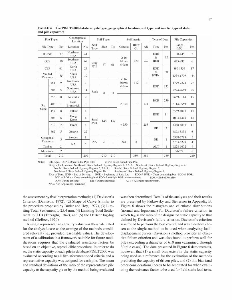
17
the assessment by five interpretation methods; (1) Davisson’sCriterion (Davisson, 1972), (2) Shape of Curve (similar tothe procedure proposed by Butler and Hoy, 1977), (3) Lim-iting Total Settlement to 25.4 mm, (4) Limiting Total Settle-ment to 0.1B (Terzaghi, 1942), and (5) the DeBeer log-logmethod (DeBeer, 1970).
A single representative capacity value was then calculatedfor the analyzed case as the average of the methods consid-ered relevant (i.e., provided reasonable value). The develop-ment of a calibration in a framework suitable for future mod-ifications requires that the evaluated resistance factors bebased on an objective, reproducible procedure. In order to doso, the static capacity of each pile in database PD/LT2000 wasevaluated according to all five aforementioned criteria and arepresentative capacity was assigned for each pile. The meanand standard deviations of the ratio of the representative pilecapacity to the capacity given by the method being evaluated
was then determined. Details of the analyses and their resultsare presented by Paikowsky and Stenerson in Appendix B.Figure 6 shows the histogram and calculated distributions(normal and lognormal) for Davisson’s failure criterion inwhich KSD is the ratio of the designated static capacity to thatdefined by Davisson’s failure criterion. Davisson’s criterionwas found to perform the best overall and was therefore cho-sen as the single method to be used when analyzing load-displacement curves. Davisson’s method provides an objec-tive failure criterion and was also found to perform well forpiles exceeding a diameter of 610 mm (examined through30 pile cases). The data presented in Figure 6 demonstrates,however, that (1) a small bias exists in the static capacitybeing used as a reference for the evaluation of the methodspredicting the capacity of driven piles, and (2) this bias (andother considerations) needs to be accounted for when evalu-ating the resistance factor to be used for field static load tests.
Pile Types Geographical
Location Soil Types Soil Inertia Type of Data Pile Capacities
Pile Type No. Location No. Soil Type
Side Tip Criteria Blow Ct.
AR Time No. Range (kN)
No.
H –Pile 37 Northeast
USA 44 0-445 2
OEP 10 Southeast
USA 69
EOD &
BOR 92
445-890
CEP 61 North USA
24
≥ 16 blows /10cm
272 ----
890-1334
Voided Concrete
35 South USA
10
Clay /Till
67 EOD
& BORs
30 1334-1779 44
254 Northwest
USA 3 1779-2224 27
305 Southwest
USA 14
< 16 blows /10cm
112 ---- EOD 135
2224-2669 25
356 8 Australia 2 2669-3114 15
406 New
Brunswick 3
Rock 0
BOR 239 3114-3559 10
457 Holland 4
≥ 350 ----- 134
3559-4003 13
508 Hong Kong
4 EOR 11
4003-4448 13
610 Israel 4 4448-4893 11
Sq. Conc
762 Ontario 22
Sand/Silt
140 < 350 ----- 255
DD 4893-5338 6
Sweden 1 5338-5783 5Octagonal Concrete
3 DR 1 5783-6228 4
Timber 2 NA 6
NA 3 1 NA 5 ----
ALT 1 6228-6672
Monotube 2 >6672 6
Total 210 210 210 210 389 389 389 210
Notes: Pile types: OEP = Open Ended Pipe Pile; CEP=Closed Ended Pipe Pile. Geographic Location: Northeast USA = Federal Highway Regions 1, 2 & 3; Southeast USA = Federal Highway Region 4;
North USA = Federal Highway Regions 5, 7 & 8; South USA = Federal Highway Region 6; Northwest USA = Federal Highway Region 10; Southwest USA = Federal Highway Region 9.
Type of Data: EOD = End of Driving; BOR = Beginning of Restrike; EOR = End of Restrike;
DD = During Driving; DR = During Restrike; ALT = Alternate measurement. NA = Non Applicable / unknown
6
17
6
2
61
11
137
9
5
1
8
8
16
5
EOD & BOR = Cases containing both EOD & BOR;EOD & BOR's = Cases containing both EOD & multiple BOR measurements;
TABLE 4 The PD/LT2000 database: pile type, geographical location, soil type, soil inertia, type of data,and pile capacities
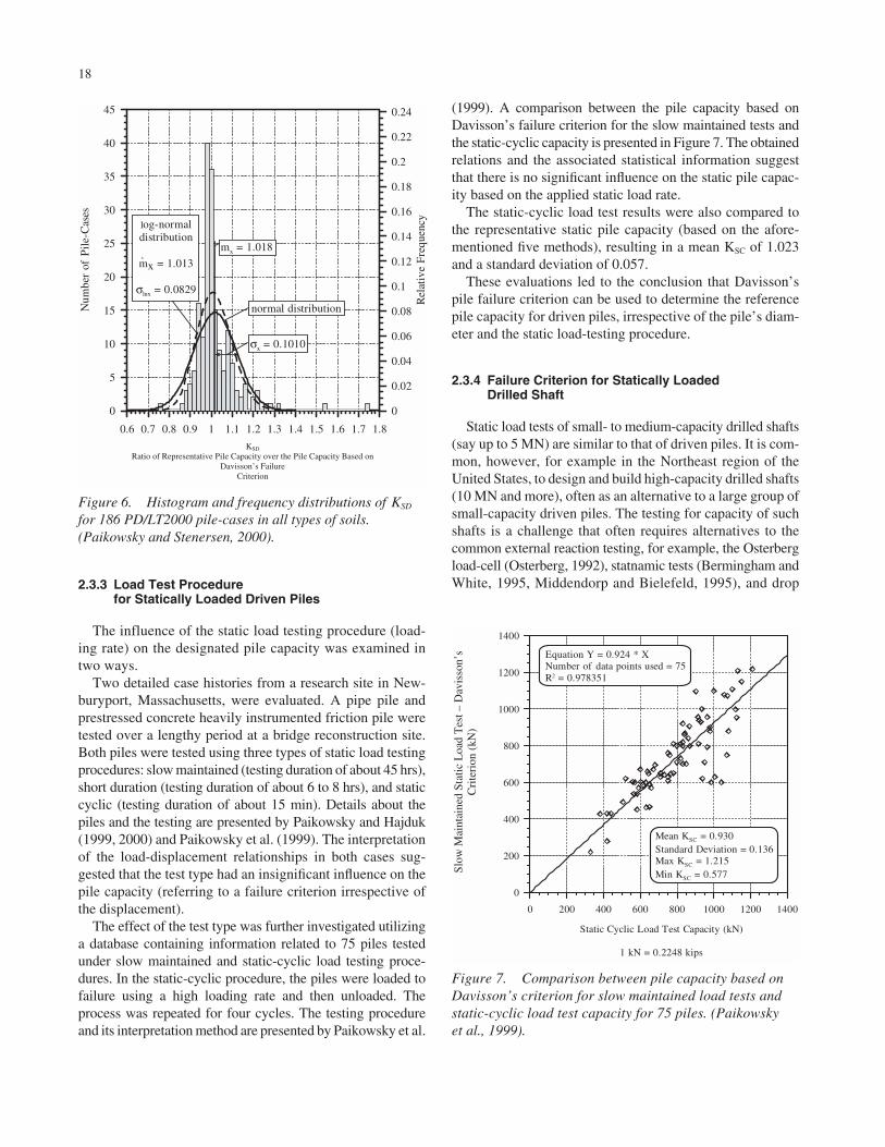
18
2.3.3 Load Test Procedure for Statically Loaded Driven Piles
The influence of the static load testing procedure (load-ing rate) on the designated pile capacity was examined intwo ways.
Two detailed case histories from a research site in New-buryport, Massachusetts, were evaluated. A pipe pile andprestressed concrete heavily instrumented friction pile weretested over a lengthy period at a bridge reconstruction site.Both piles were tested using three types of static load testingprocedures: slow maintained (testing duration of about 45 hrs),short duration (testing duration of about 6 to 8 hrs), and staticcyclic (testing duration of about 15 min). Details about thepiles and the testing are presented by Paikowsky and Hajduk(1999, 2000) and Paikowsky et al. (1999). The interpretationof the load-displacement relationships in both cases sug-gested that the test type had an insignificant influence on thepile capacity (referring to a failure criterion irrespective ofthe displacement).
The effect of the test type was further investigated utilizinga database containing information related to 75 piles testedunder slow maintained and static-cyclic load testing proce-dures. In the static-cyclic procedure, the piles were loaded tofailure using a high loading rate and then unloaded. Theprocess was repeated for four cycles. The testing procedureand its interpretation method are presented by Paikowsky et al.
(1999). A comparison between the pile capacity based onDavisson’s failure criterion for the slow maintained tests andthe static-cyclic capacity is presented in Figure 7. The obtainedrelations and the associated statistical information suggestthat there is no significant influence on the static pile capac-ity based on the applied static load rate.
The static-cyclic load test results were also compared tothe representative static pile capacity (based on the afore-mentioned five methods), resulting in a mean KSC of 1.023and a standard deviation of 0.057.
These evaluations led to the conclusion that Davisson’spile failure criterion can be used to determine the referencepile capacity for driven piles, irrespective of the pile’s diam-eter and the static load-testing procedure.
2.3.4 Failure Criterion for Statically LoadedDrilled Shaft
Static load tests of small- to medium-capacity drilled shafts(say up to 5 MN) are similar to that of driven piles. It is com-mon, however, for example in the Northeast region of theUnited States, to design and build high-capacity drilled shafts(10 MN and more), often as an alternative to a large group ofsmall-capacity driven piles. The testing for capacity of suchshafts is a challenge that often requires alternatives to thecommon external reaction testing, for example, the Osterbergload-cell (Osterberg, 1992), statnamic tests (Bermingham andWhite, 1995, Middendorp and Bielefeld, 1995), and drop
0.6 0.7 0.8 0.9 1 1.1 1.2 1.3 1.4 1.5 1.6 1.7 1.8
0
5
10
15
20
25
30
35
40
45
Num
ber
of P
ile-
Cas
es
0
0.02
0.04
0.06
0.08
0.1
0.12
0.14
0.16
0.18
0.2
0.22
0.24
Rel
ativ
e F
requ
encylog-normal
distribution
^mx = 1.013
σlnx = 0.0829
normal distribution
mx = 1.018
σx = 0.1010
KSD
Ratio of Representative Pile Capacity over the Pile Capacity Based on Davisson’s Failure
Criterion
0 200 400 600 800 1000 1200 1400
Static Cyclic Load Test Capacity (kN)
1 kN = 0.2248 kips
0
200
400
600
800
1000
1200
1400
Equation Y = 0.924 * XNumber of data points used = 75R2 = 0.978351
Mean KSC = 0.930Standard Deviation = 0.136Max KSC = 1.215Min KSC = 0.577S
low
Mai
ntai
ned
Sta
tic
Loa
d T
est –
Dav
isso
n’s
Cri
teri
on (
kN)
Figure 6. Histogram and frequency distributions of KSD
for 186 PD/LT2000 pile-cases in all types of soils.(Paikowsky and Stenersen, 2000).
Figure 7. Comparison between pile capacity based onDavisson’s criterion for slow maintained load tests andstatic-cyclic load test capacity for 75 piles. (Paikowsky et al., 1999).
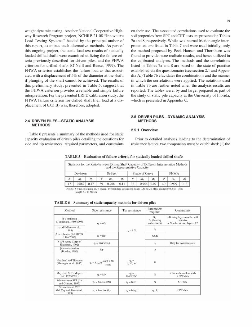
19
weight dynamic testing. Another National Cooperative High-way Research Program project, NCHRP-21-08 “InnovativeLoad Testing Systems,” headed by the principal author ofthis report, examines such alternative methods. As part ofthis ongoing project, the static load-test results of staticallyloaded drilled shafts were examined utilizing the failure cri-teria previously described for driven piles, and the FHWAcriterion for drilled shafts (O’Neill and Reese, 1999). TheFHWA criterion establishes the failure load as that associ-ated with a displacement of 5% of the diameter at the shaft,if plunging of the shaft cannot be achieved. The results ofthis preliminary study, presented in Table 5, suggest thatthe FHWA criterion provides a reliable and simple failureinterpretation. For the presented LRFD calibration study, theFHWA failure criterion for drilled shaft (i.e., load at a dis-placement of 0.05 B) was, therefore, adopted.
2.4 DRIVEN PILES—STATIC ANALYSISMETHODS
Table 6 presents a summary of the methods used for staticcapacity evaluation of driven piles detailing the equations forside and tip resistances, required parameters, and constraints
on their use. The associated correlations used to evaluate thesoil properties from SPT and CPT tests are presented in Tables7a and 8, respectively. While two internal friction angle inter-pretations are listed in Table 7 and were used initially, onlythe method proposed by Peck Hansen and Thornburn wasfound to provide more realistic results, and hence utilized inthe calibrated analyses. The methods and the correlationslisted in Tables 7a and 8 are based on the state of practiceestablished via the questionnaire (see section 2.1 and Appen-dix A.) Table 7b elucidates the combinations and the mannerin which the correlations were applied. The notations usedin Table 7b are further noted when the analysis results arereported. The tables were, by and large, prepared as part ofthe study of static pile capacity at the University of Florida,which is presented in Appendix C.
2.5 DRIVEN PILES—DYNAMIC ANALYSISMETHODS
2.5.1 Overview
Prior to detailed analyses leading to the determination ofresistance factors, two components must be established: (1) the
Statistics for the Ratio between Drilled Shaft Capacity of Different Interpretation Methods and the Representative Capacity
Davisson DeBeer Shape of Curve FHWA
# mx σx # mx σx # mx σx # mx σx
47 0.862 0.17 39 0.908 0.11 36 0.956 0.09 40 0.999 0.13
Notes: # = no. of cases; mx = mean; σx=standard deviation; loads 0.85 to 20 MN; diameter 0.3 to 1.5m; length 5.3 to 58.5m
Method Side resistance Tip resistance Parameters required Constraints
α-Tomlinson (Tomlinson, 1980/1995)
Su; Db (bearing embedment)
+Bearing layer must be stiff cohesive
+ Number of soil layers ≤ 2 α-API (Reese et al.,
1998)
qs = αSu
Su
β in cohesive (AASHTO, 1996/2000) qs = βσ’
λ (US Army Corps of Engineers, 1992)
qs = λ(σ’+2Su)
qp = 9 Su
Su Only for cohesive soils
β in cohesionless (Bowles, 1996) βσ’ Dr
Nordlund and Thurman (Hannigan et al., 1995) ϖ
ϖ+δσ= δ cos
)sin(’CKq Fs
qp = αt N’q σ’ φ
Meyerhof SPT (Meyer-hof, 1976/1981)
qs = k N qp = 0.4D/BN’
N + For cohesionless soils + SPT data
Schmertmann SPT (Lai and Graham, 1995) qs = function(N) qp = fn(N) N SPTdata
Schmertmann CPT (McVay and Townsend,
1989) qs = function(fs) p = fn(qc) c, fs CPT data
OCR
q q
TABLE 6 Summary of static capacity methods for driven piles
TABLE 5 Evaluation of failure criteria for statically loaded drilled shafts
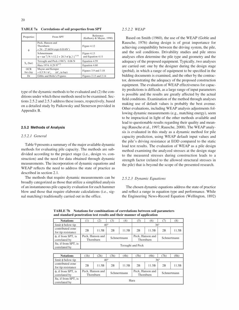
20
type of the dynamic methods to be evaluated and (2) the con-ditions under which these methods need to be examined. Sec-tions 2.5.2 and 2.5.3 address these issues, respectively, basedon a detailed study by Paikowsky and Stenerson provided inAppendix B.
2.5.2 Methods of Analysis
2.5.2.1 General
Table 9 presents a summary of the major available dynamicmethods for evaluating pile capacity. The methods are sub-divided according to the project stage (i.e., design vs. con-struction) and the need for data obtained through dynamicmeasurements. The incorporation of dynamic equations andWEAP reflects the need to address the state of practice asdescribed in section 2.1.
The methods that require dynamic measurements can bebroadly categorized as those that utilize a simplified analysisof an instantaneous pile capacity evaluation for each hammerblow and those that require elaborate calculations (i.e., sig-nal matching) traditionally carried out in the office.
2.5.2.2 WEAP
Based on Smith (1960), the use of the WEAP (Goble andRausche, 1976) during design is of great importance forachieving compatibility between the driving system, the pile,and the soil conditions. Drivability studies and pile stressanalyses often determine the pile type and geometry and theadequacy of the proposed equipment. Typically, two analysesare carried out: one by the designer during the design stage(prebid), in which a range of equipment to be specified in thebidding documents is examined, and the other by the contrac-tor, demonstrating the adequacy of the proposed constructionequipment. The evaluation of WEAP effectiveness for capac-ity predictions is difficult, as a large range of input parametersis possible and the results are greatly affected by the actualfield conditions. Examination of the method through analysesmaking use of default values is probably the best avenue.Other evaluations, including WEAP analysis adjustments fol-lowing dynamic measurements (e.g., matching energy), seemto be impractical in light of the other methods available andlead to questionable results regarding their quality and mean-ing (Rausche et al., 1997; Rausche, 2000). The WEAP analy-sis is evaluated in this study as a dynamic method for pilecapacity prediction, using WEAP default input values andthe pile’s driving resistance at EOD compared to the staticload test results. The evaluation of WEAP as a pile designmethod examining the analyzed stresses at the design stageto the measured stresses during construction leads to astrength factor (related to the allowed structural stresses inthe pile) that is beyond the scope of the presented research.
2.5.2.3 Dynamic Equations
The chosen dynamic equations address the state of practiceand reflect a range in equation type and performance. Whilethe Engineering News-Record Equation (Wellington, 1892)
Properties From SPT Reference (Kulhawy & Mayne, 1990)
Peck, Hanson and Thornburn: ≈ 54 - 27.6034 exp(-0.014N’)
Figure 4.12
φ Schmertmann ϕ ≈ tan-1[ N / (12.2 + 20.3 σ’/pa’) ]
0.34 Figure 4.13 and Equation 4.11
Terzaghi and Peck (1967): 0.06 N Equation 4.59 Su (bar)
Hara 1974: 0.29 N0.72 Equation 4.60 OCR
for clay Mayne and Kemper ≈ 0.5 N / σ’o (σ’o in bar)
Figures 3.9 and 3.18
Dr Gibbs and Holtz's F igures Figures 2.13 and 2.14
Notations (1) (2) (3) (4) (5) (6) (7) (8) limit φ below tip 40° 36° contributed zone for tip resistance
2B 11.5B 2B 11.5B 2B 11.5B 2B 11.5B
φ, if from SPT, is correlated by
Peck, Hanson and Thornburn
Schmertmann Peck, Hanson and
Thornburn Schmertmann
Su, if from SPT, is correlated by
Terzaghi and Peck
Notations (1h) (2h) (3h) (4h) (5h) (6h) (7h) (8h) limit φ below tip 40° 36° contributed zone for tip resistance
2B 11.5B 2B 11.5B 2B 11.5B 2B 11.5B
φ, if from SPT, is correlated by
Peck, Hanson and Thornburn
Schmertmann Peck, Hanson and
Thornburn Schmertmann
Su, if from SPT, is correlated by
Hara
TABLE 7a Correlations of soil properties from SPT
TABLE 7b Notations for combinations of correlations between soil parameters and standard penetration test results and their manner of application
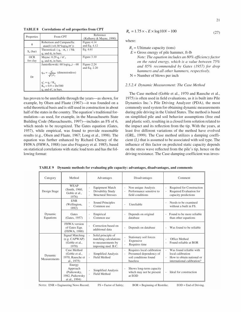
21
has proven to be unreliable through the years—as shown, forexample, by Olsen and Flaate (1967)—it was founded on asolid theoretical basis and is still used in construction in abouthalf of the states in the country. The equation’s traditional for-mulation—as used, for example, in the Massachusetts StateBuilding Code (Massachusetts, 1997)—includes an FS of 6,which needs to be recognized. The Gates equation (Gates,1957), while empirical, was found to provide reasonableresults (e.g., Olsen and Flaate, 1967; Long et al., 1998). Theequation was further enhanced by Richard Cheney of theFHWA (FHWA, 1988) (see also Fragaszy et al. 1985), basedon statistical correlations with static load tests and has the fol-lowing format:
(27)
where:
Ru = Ultimate capacity (tons)E = Gross energy of pile hammer, ft-lb
Note: The equation includes an 80% efficiency factoron the rated energy, which is a value between 75%and 85% recommended by Gates (1957) for drophammers and all other hammers, respectively.
N = Number of blows per inch
2.5.2.4 Dynamic Measurement: The Case Method
The Case method (Goble et al., 1970 and Rausche et al.,1975) is often used in field evaluations, as it is built into PileDynamics Inc.’s Pile Driving Analyzer (PDA), the mostcommonly used system for obtaining dynamic measurementsduring pile driving in the United States. The method is basedon simplified pile and soil behavior assumptions (free endand plastic soil), resulting in a closed form solution related tothe impact and its reflection from the tip. With the years, atleast five different variations of the method have evolved(GRL, 1999). The Case method utilizes a damping coeffi-cient (Jc) that is assumed to be associated with soil type. Theinfluence of this factor on predicted static capacity dependson the stress wave reflected from the pile’s tip, hence on thedriving resistance. The Case-damping coefficient was inves-
R E Nu = × × −1 75 10 100. logProperties From CPT
Reference (Kulhawy & Mayne, 1990)
φ Robertson and Campanella: atan(0.1+0.38*log(qc/σ’))
Figure 4.14 and Eq. 4.12
Su (bar) Theoretical: ( qc - σo ) / Nk qc and σo in bars.
Eq. 4.61
OCR for clay
Mayne: 0.29 qc / σ’o qc and σo in bars.
Figure 3.10
Dr
Jamiolkowski: 68 log(qcn) – 68
qcn = 0a
c
’P
’q
σ (dimensionless)
q’c = qc / Kq Kq = 0.9 + Dr/300 qc and σ’o in bars.
Figure 2.24 and Eq. 2.20
TABLE 8 Correlations of soil properties from CPT
Category Method Advantages Disadvantages Comment
Design Stage
WEAP (Smith, 1960, Goble et al.,
1976)
- Equipment Match - Drivability Study - Structural Stresses
- Non unique Analysis - Performance sensitive to
field conditions
- Required for Construction - Required Evaluation for
capacity predictions
ENR (Wellington,
1892)
- Sound Principles - Common use
- Unreliable - Needs to be examined
without a built in FS.
Gates (Gates, 1957)
- Empirical - Common use
- Depends on original database
- Found to be more reliable than other equations
Dynamic Equations
FHWA version of Gates Eqn.
(FHWA, 1988)
- Correction based on additional data
- Depends on database - Was found to be reliable
Signal Matching (e.g. CAPWAP)
(Goble et al., 1970)
- Solid principle of matching calculations to measurements by imposing msd. B.C.
- Stationary soil forces - Expensive - Requires time
- Office Method - Found reliable at BOR
Case Method (Goble et al.,
1970, Rausche et al., 1975)
- Simplified Analysis - Field Method
- Requires local calibration - Presumed dependency of
soil conditions found baseless
- Was found reliable with local calibration
- How to obtain national or international calibration?
Dynamic Measurements
Energy Approach
(Paikowsky, 1982, Paikowsky
et al., 1994)
- Simplified Analysis - Field Method
- Shows long-term capacity which may not be present at EOD
- Ideal for construction
NOTES: ENR = Engineering News Record; FS = Factor of Safety; BOR = Beginning of Restrike; EOD = End of Driving.
TABLE 9 Dynamic methods for evaluating pile capacity: advantages, disadvantages, and comments
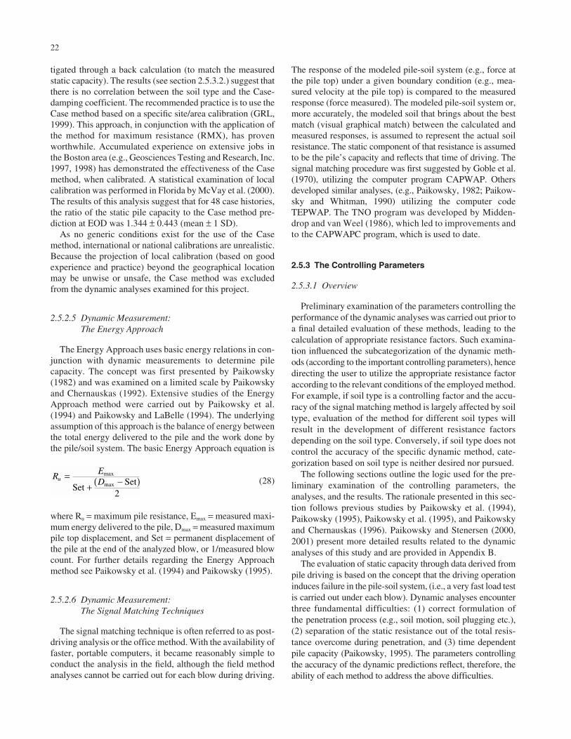
22
tigated through a back calculation (to match the measuredstatic capacity). The results (see section 2.5.3.2.) suggest thatthere is no correlation between the soil type and the Case-damping coefficient. The recommended practice is to use theCase method based on a specific site/area calibration (GRL,1999). This approach, in conjunction with the application ofthe method for maximum resistance (RMX), has provenworthwhile. Accumulated experience on extensive jobs inthe Boston area (e.g., Geosciences Testing and Research, Inc.1997, 1998) has demonstrated the effectiveness of the Casemethod, when calibrated. A statistical examination of localcalibration was performed in Florida by McVay et al. (2000).The results of this analysis suggest that for 48 case histories,the ratio of the static pile capacity to the Case method pre-diction at EOD was 1.344 ± 0.443 (mean ± 1 SD).
As no generic conditions exist for the use of the Casemethod, international or national calibrations are unrealistic.Because the projection of local calibration (based on goodexperience and practice) beyond the geographical locationmay be unwise or unsafe, the Case method was excludedfrom the dynamic analyses examined for this project.
2.5.2.5 Dynamic Measurement: The Energy Approach
The Energy Approach uses basic energy relations in con-junction with dynamic measurements to determine pilecapacity. The concept was first presented by Paikowsky(1982) and was examined on a limited scale by Paikowskyand Chernauskas (1992). Extensive studies of the EnergyApproach method were carried out by Paikowsky et al.(1994) and Paikowsky and LaBelle (1994). The underlyingassumption of this approach is the balance of energy betweenthe total energy delivered to the pile and the work done bythe pile/soil system. The basic Energy Approach equation is
(28)
where Ru = maximum pile resistance, Emax = measured maxi-mum energy delivered to the pile, Dmax = measured maximumpile top displacement, and Set = permanent displacement ofthe pile at the end of the analyzed blow, or 1/measured blowcount. For further details regarding the Energy Approachmethod see Paikowsky et al. (1994) and Paikowsky (1995).
2.5.2.6 Dynamic Measurement: The Signal Matching Techniques
The signal matching technique is often referred to as post-driving analysis or the office method. With the availability offaster, portable computers, it became reasonably simple toconduct the analysis in the field, although the field methodanalyses cannot be carried out for each blow during driving.
REDu =
+ −( )max
maxSetSet
2
The response of the modeled pile-soil system (e.g., force atthe pile top) under a given boundary condition (e.g., mea-sured velocity at the pile top) is compared to the measuredresponse (force measured). The modeled pile-soil system or,more accurately, the modeled soil that brings about the bestmatch (visual graphical match) between the calculated andmeasured responses, is assumed to represent the actual soilresistance. The static component of that resistance is assumedto be the pile’s capacity and reflects that time of driving. Thesignal matching procedure was first suggested by Goble et al.(1970), utilizing the computer program CAPWAP. Othersdeveloped similar analyses, (e.g., Paikowsky, 1982; Paikow-sky and Whitman, 1990) utilizing the computer codeTEPWAP. The TNO program was developed by Midden-drop and van Weel (1986), which led to improvements andto the CAPWAPC program, which is used to date.
2.5.3 The Controlling Parameters
2.5.3.1 Overview
Preliminary examination of the parameters controlling theperformance of the dynamic analyses was carried out prior toa final detailed evaluation of these methods, leading to thecalculation of appropriate resistance factors. Such examina-tion influenced the subcategorization of the dynamic meth-ods (according to the important controlling parameters), hencedirecting the user to utilize the appropriate resistance factoraccording to the relevant conditions of the employed method.For example, if soil type is a controlling factor and the accu-racy of the signal matching method is largely affected by soiltype, evaluation of the method for different soil types willresult in the development of different resistance factorsdepending on the soil type. Conversely, if soil type does notcontrol the accuracy of the specific dynamic method, cate-gorization based on soil type is neither desired nor pursued.
The following sections outline the logic used for the pre-liminary examination of the controlling parameters, theanalyses, and the results. The rationale presented in this sec-tion follows previous studies by Paikowsky et al. (1994),Paikowsky (1995), Paikowsky et al. (1995), and Paikowskyand Chernauskas (1996). Paikowsky and Stenersen (2000,2001) present more detailed results related to the dynamicanalyses of this study and are provided in Appendix B.
The evaluation of static capacity through data derived frompile driving is based on the concept that the driving operationinduces failure in the pile-soil system, (i.e., a very fast load testis carried out under each blow). Dynamic analyses encounterthree fundamental difficulties: (1) correct formulation ofthe penetration process (e.g., soil motion, soil plugging etc.),(2) separation of the static resistance out of the total resis-tance overcome during penetration, and (3) time dependentpile capacity (Paikowsky, 1995). The parameters controllingthe accuracy of the dynamic predictions reflect, therefore, theability of each method to address the above difficulties.
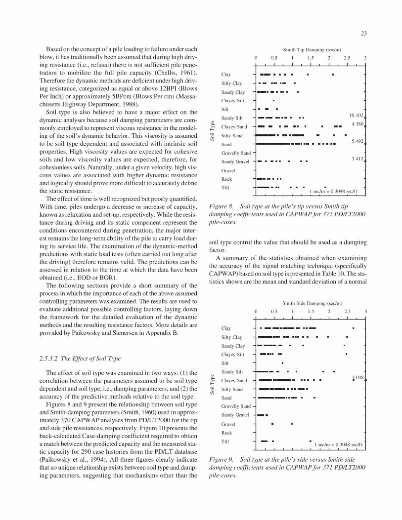
23
Based on the concept of a pile loading to failure under eachblow, it has traditionally been assumed that during high driv-ing resistance (i.e., refusal) there is not sufficient pile pene-tration to mobilize the full pile capacity (Chellis, 1961).Therefore the dynamic methods are deficient under high driv-ing resistance, categorized as equal or above 12BPI (BlowsPer Inch) or approximately 5BPcm (Blows Per cm) (Massa-chusetts Highway Department, 1988).
Soil type is also believed to have a major effect on thedynamic analyses because soil damping parameters are com-monly employed to represent viscous resistance in the model-ing of the soil’s dynamic behavior. This viscosity is assumedto be soil type dependent and associated with intrinsic soilproperties. High viscosity values are expected for cohesivesoils and low viscosity values are expected, therefore, forcohesionless soils. Naturally, under a given velocity, high vis-cous values are associated with higher dynamic resistanceand logically should prove more difficult to accurately definethe static resistance.
The effect of time is well recognized but poorly quantified.With time, piles undergo a decrease or increase of capacity,known as relaxation and set-up, respectively. While the resis-tance during driving and its static component represent theconditions encountered during penetration, the major inter-est remains the long-term ability of the pile to carry load dur-ing its service life. The examination of the dynamic-methodpredictions with static load tests (often carried out long afterthe driving) therefore remains valid. The predictions can beassessed in relation to the time at which the data have beenobtained (i.e., EOD or BOR).
The following sections provide a short summary of theprocess in which the importance of each of the above assumedcontrolling parameters was examined. The results are used toevaluate additional possible controlling factors, laying downthe framework for the detailed evaluation of the dynamicmethods and the resulting resistance factors. More details areprovided by Paikowsky and Stenersen in Appendix B.
2.5.3.2 The Effect of Soil Type
The effect of soil type was examined in two ways: (1) thecorrelation between the parameters assumed to be soil typedependent and soil type, i.e., damping parameters; and (2) theaccuracy of the predictive methods relative to the soil type.
Figures 8 and 9 present the relationship between soil typeand Smith-damping parameters (Smith, 1960) used in approx-imately 370 CAPWAP analyses from PD/LT2000 for the tipand side pile resistances, respectively. Figure 10 presents theback-calculated Case-damping coefficient required to obtaina match between the predicted capacity and the measured sta-tic capacity for 290 case histories from the PD/LT database(Paikowsky et al., 1994). All three figures clearly indicatethat no unique relationship exists between soil type and damp-ing parameters, suggesting that mechanisms other than the
soil type control the value that should be used as a dampingfactor.
A summary of the statistics obtained when examiningthe accuracy of the signal matching technique (specificallyCAPWAP) based on soil type is presented in Table 10. The sta-tistics shown are the mean and standard deviation of a normal
0 0.5 1 1.5 2 2.5 3
Smith Tip Damping (sec/m)
Soi
l T
ype
Gravelly Sand
Sandy Gravel
Clayey Sand
Clay
Silty Clay
Sandy Clay
Clayey Silt
Silt
Sandy Silt
Silty Sand
Sand
Gravel
Rock
Till1 sec/m = 0.3048 sec/f t
5.492
3.412
10.102
4.380
0 0.5 1 1.5 2 2.5 3
Smith Side Damping (sec/m)
Soi
l T
ype
Gravelly Sand
Sandy Gravel
Clayey Sand
Clay
Silty Clay
Sandy Clay
Clayey Silt
Silt
Sandy Silt
Silty Sand
Sand
Gravel
Rock
Till1 sec/m = 0.3048 sec/f t
3.048
Figure 8. Soil type at the pile’s tip versus Smith tipdamping coefficients used in CAPWAP for 372 PD/LT2000pile-cases.
Figure 9. Soil type at the pile’s side versus Smith sidedamping coefficients used in CAPWAP for 371 PD/LT2000pile-cases.
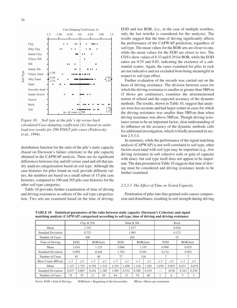
24
distribution function for the ratio of the pile’s static capacity(based on Davisson’s failure criterion) to the pile capacityobtained in the CAPWAP analysis. There are no significantdifferences between clay and till versus sand and silt that jus-tify analysis categorization based on soil type. Although thecase histories for piles found on rock provide different val-ues, the numbers are based on a small subset of 15 pile casehistories, compared to 100 and 265 pile case histories for theother soil type categories.
Table 10 provides further examination of time of drivingand driving resistances as subsets of the soil type categoriza-tion. Two sets are examined based on the time of driving:
EOD and last BOR, (i.e., in the case of multiple restrikes,only the last restrike is considered for the analysis). Theresults suggest that the time of driving significantly affectsthe performance of the CAPWAP prediction, regardless ofsoil type. The mean values for the BOR sets are closer to one,while the mean values for the EOD are closer to two. TheCOVs show values of 0.33 and 0.39 for BOR, while the EODratios are 0.55 and 0.85, indicating the existence of a sub-stantial scatter. Again, the cases examined for piles in rockare not indicative and are excluded from being meaningful inrespect to soil type effect.
Further evaluation of the records was carried out on thebasis of driving resistance. The division between cases forwhich the driving resistance is smaller or greater than 5BPcm(5 blows per centimeter), examines the aforementionednotion of refusal and the expected accuracy of the dynamicmethods. The results, shown in Table 10, suggest that analy-ses were less accurate and had larger scatter in cases for whichthe driving resistance was smaller than 5BPcm than whendriving resistance was above 5BPcm. Though driving resis-tance seems to be an important factor, clear understanding ofits influence on the accuracy of the dynamic methods callsfor additional investigation, which is briefly presented in sec-tion 2.5.3.4.
In summary, while the performance of the signal matchinganalysis (CAPWAP) is not well correlated to soil type, otherfactors associated with soil type may be important (e.g., lowdriving resistance in soft cohesive soils or gain of capacitywith time); but soil type itself does not appear to be impor-tant. The data presented in Table 10 suggests that time of driv-ing must be considered and driving resistance needs to befurther examined.
2.5.3.3 The Effect of Time on Tested Capacity
Penetration of piles into fine-grained soils causes compres-sion and disturbance, resulting in soil strength during driving
Soi
l T
ype
Clay
Silty Clay
Sandy Clay
Clayey Silt
Silt
Sandy Silt
Clayey Sand
Silty Sand
Sand
Gravelly Sand
Sandy Gravel
Gravel
Rock
Till
-1.86
-5.04-2.25
7.041.51
1.562.22no. of cases = 290
-1.5 0.0 1.5-1.00 -0.50 0.50 1.00
Case Damping Coeff icient, Jc
Figure 10. Soil type at the pile’s tip versus backcalculated Case-damping coefficient (Jc) based on staticload test results for 290 PD/LT pile-cases (Paikowsky et al., 1994).
Clay & Till Sand & Silt Rock
Mean 1.352 1.517 0.930
Standard Deviation 0.723 1.085 0.172
Number of Cases 100 265 15
Time of Driving EOD BOR(last) EOD BOR(last) EOD BOR(last)
Mean 1.634 1.133 2.068 1.193 0.968 0.925
Standard Deviation 0.899 0.444 1.765 0.391 0.132 0.203
Number of Cases 45 40 77 116 7 7
Blow Count (BPcm) < 5 ≥ 5 < 5 ≥ 5 < 5 ≥ 5 < 5 ≥ 5 < 5 ≥ 5 < 5 ≥ 5
Mean 1.127 1.725 0.750 1.315 2.191 1.458 1.126 1.283 1.070 0.952 0.671 0.879
Standard Deviation 0.637 0.807 0.241 1.160 1.901 0.512 0.386 0.355 ----- 0.136 0.163 0.230
Number of Cases 35 35 11 10 64 13 74 40 1 6 3 3
NOTES: EOD = End of Driving; BOR(last) = Beginning of the last restrike; BPcm = Blows per centimeter
TABLE 10 Statistical parameters of the ratio between static capacity (Davisson’s Criterion) and signalmatching analysis (CAPWAP) categorized according to soil type, time of driving and driving resistance

25
that differs from its long-term strength, thus affecting pilecapacity. Although factors such as thixotropy and aging con-tribute to this phenomenon, the migration of pore water is themost significant cause of capacity gain with time. Measure-ments carried out on a model (Paikowsky and Hart, 2000) andfull-scale piles (Paikowsky and Hajduk, 1999, 2000) showthat pore pressure at magnitudes similar to the total soil pres-sure creates in clays around the pile’s shaft zones of aboutzero effective stress, resulting in almost a complete loss offrictional resistance. Paikowsky et al. (1995, 1996) examinedthe static and dynamic gain of capacity with time based onradial consolidation; a normalization process was followed,allowing for comparison between different pile sizes.
Table 11 presents a summary of parameters describingthe pile capacity gain with time based on static and dynamictesting. The slope of the relation between the static capac-ity and the maximum static capacity (scale of 0 to 1) to theelapsed time after driving (logarithm scale) for a 152.4 mmradius (1 ft diameter) pile is denoted as Cgt. Similar relationsfor the ratio of dynamic capacity (with time) to the maximumstatic capacity result in a slope denoted by the parameter Cgtd.The time required for the standard pile to gain 75% of its max-imum capacity is denoted as t75. The time extrapolation forany desired pile size is achieved through the relationship of
t75 (pile) = 4r2 t75 (table) (29)
For which r = the desired pile radius (ft.) or its equivalentfor a pile of different shape.
The data in Table 11 show that while the rate of capacitygain is similar according to both analyses (Cgt = 0.389, Cgtd =0.348), the associated time for achieving 75% of the maxi-mum capacity (normalized for all piles to 304.8 mm diame-ter) is about 20 times greater when analyzed by static meth-ods than when analyzed by dynamic methods. In other words,dynamic testing and analyses (namely CAPWAP), while fol-lowing the physical behavior of capacity gain, exhibit thisgain much faster than the actual gain monitored by the staticload test results. The ramifications of these conclusions arethat (1) actual gain of capacity is much slower than that exhib-ited by the dynamic methods, (2) scheduling of constructionor testing based on capacity gain should consider the reason
for time evaluation (i.e., actual loading in construction ordynamic testing as part of quality control), and (3) at present,the dynamic methods evaluation should concentrate on thelong-term pile capacity.
2.5.3.4 The Effect of Soil Motion
Overview. Paikowsky and Chernauskas (1996) show that thestationary soil assumption, under which the soil/pile interac-tion models were developed, does not reflect the physicalphenomenon that occurs during pile driving. Pseudo-viscousdamping serves as a mechanism to absorb energy; but, as itdoes not reflect the actual phenomenon, it cannot be corre-lated to physical properties (e.g., soil type) or time of driving.If the motion of the displaced soil is a major factor con-tributing to energy loss during driving, a substantial portionof the dynamic resistance should be a function of two param-eters: (1) acceleration of the displaced soil (especially at thetip) that can be conveniently examined as a function of thedriving resistance, and (2) mass/volume of the displaced soilthat is a function of the pile geometry, namely, small vs. largedisplacement piles. A brief summary of the findingsdescribed by Paikowsky and Stenersen regarding the abovetwo factors follows. Further details of their research are pro-vided in Appendix B.
Soil Acceleration/Driving Resistance. The energy lossthrough the work performed by the displaced soil mass atthe tip is directly related to the acceleration of this mass. Thedetailed evaluation of the soil’s motion at the tip is beyond thescope of the present research and is described by Hölscher(1995), Hölscher and Barends (1996), and Hajduk et al.(2000). The indirect evaluation of these accelerations can beperformed through analysis of the driving resistance, whichis the measure of the pile’s final displacement under eachhammer blow. With low driving resistance (easy driving),high acceleration and velocity (i.e., free-end analogy) aredeveloped at the tip. In the case of high driving resistance(hard driving), there is small acceleration at the tip, resultingin little, if any, mobilization of the soil mass beyond a radi-ating elastic wave. The corresponding energy loss due to soilmotion is, therefore, small.
Static Data Sets LTT and PUT/LTT
Dynamic Data Set PD/LTT ALL DATA
Cgt t75* gtd t75** gt t75**
No. of Cases 15 5 7 6 22 11
Average for all piles in set.
0.389 385.0 0.348 21.3 0.376 186.6
Standard De-viation
0.119 226.3 0.068 7.9 0.106 237.9
C C
Notes: *closed-ended pipe piles only; **t75 = time for a standard pile (0.3048m radius) to gain 75% of its maximum capacity; Cgt = rate of pile capacity gain with the logarithm of time
TABLE 11 Summary of static-and-dynamic-based capacity gain with time parameters based on data sets (Paikowsky et al. 1996)

26
To evaluate the blow count that identifies the transitionbetween easy and hard driving (high and low soil acceleration)the ratio between the static capacity and the CAPWAP pre-diction (KSW) by blow count for all pile case histories inPD/LT2000 was determined, as presented in Figure 11a. Fig-ure 11b presents the data separated into intervals of 8 BP10cm(2BPI), with the mean and standard deviation of each groupgraphed as a point and an error bar against the mid point blowcount of the interval. For example, for driving resistancebetween 0 and 8BP10cm there were 42 case histories with amean of 2.506 and a standard deviation of 2.217 plotted atthe center of the interval, i.e., at 4BP10cm. The data pre-sented in Figure 11b show that for the first two intervals (upto 16BP10cm) the predicted capacity was substantially lowerthan for all other intervals with a significantly higher scatter.After approximately 16 blows per 10cm, the mean and stan-dard deviation of the individual intervals fall within the rangeof all case histories. The boundary of the dynamic methodevaluation based on driving resistance was defined, there-fore, as 16BP10cm (4BPI).
Displaced Soil/Pile Area Ratio. The volume of the displacedsoil is identical to the volume of the penetrating pile, except
when pile plugging takes place (Paikowsky and Whitman,1990). The piles, therefore, can be classified as small (e.g., Hand unplugged open pipe) and large (e.g., closed pipe andsquare concrete) displacement piles. Additional classificationof open-pipe piles can be made according to a tip-area ratiosimilar to that used for soil samplers (Paikowsky et al., 1989).
As most soil displacement takes place at the tip area, theclassification of piles can be better served by looking at theratio between the pile’s embedded surface area and the areaof the pile tip (Paikowsky et al., 1994):
(30)
Using this ratio, a pile traditionally referred to as a “large dis-placement” pile can behave like a “small displacement pile” ifit is driven deeply enough. A quantitative boundary of AR =350 between “small” and “large” displacement piles was pro-posed by Paikowsky et al. (1994).
Figure 12a presents the relationship between AR and theratio of the static capacity over CAPWAP prediction (KSW)for all pile case histories in PD/LT2000. The data are sepa-rated into AR intervals of 175, with the mean and standarddeviation of each group graphed as a point and error bar at
AAAR
skin
tip= = Surface area in contact with soil
Area of pile tip
(a)
(b)
0 8 16 24 32 40 48 56 64 72 80 88
Blow Count (blows/10cm)
0
1
2
3
4
KS
W
0 2 4 6 8 10 12 14 16 18 20Blow Count (blows/inch)
0 40 80 120 160 200 240 280 320 360 400
Blow Count (blows/10cm)
0
1
2
3
4
KS
W =
L
oad
Tes
t R
esul
tsC
AP
WA
P or
TE
PW
AP
Pre
dict
ions 0 10 20 30 40 50 60 70 80 90 100
Blow Count (blows/in)
no set
no set
42
6664 38 32
2515 16 8 16 60
no. of cases in8 blows/10cm interval
mean for all cases = 1.452
standard deviation for all cases = 0.985
Total no. of cases = 382
6.85, 11.26, 5.97, 9.38, 5.26, 4.75, 4.41
4.72
LG SMDISP DISP Sand & Silt Clay & Till Rock
Figure 11. The ratio of static capacity to dynamic signalmatching prediction, KSW versus blow count for all pile-cases in PD/LT2000 (a) all data points, and (b) datagrouped in intervals of 8 blows/10cm (2BPI).
0 175 350 525 700 875 1050 1225 1400 1575Area Ratio, AR
0
1
2
3
4
KSW
=
L
oad
Tes
t Res
ults
CA
PW
AP
or
TE
PW
AP
Pre
dict
ions
111139
18 12 115
37
no. of cases inintervals of 175
mean for all cases = 1.452
standard deviation for all cases = 0.985
Total no. of cases = 382
76
0 1050 2100 3150Area Ratio, AR
0
1
2
3
4
KSW
=
L
oad
Tes
t Res
ults
CA
PW
AP
or
TE
PW
AP
Pre
dict
ions
16 21
6 8 10
10
no. of casesin intervals
mean for all cases = 1.460
standard deviation for all cases = 0.734
Total no. of cases = 71
175350525
(b)
(a)
Figure 12. KSW versus area ratio, (a) for all pile-cases inPD/LT2000 and (b) for 71 pile-cases with drivingresistance exceeding 16 BP10cm (4BPI) at the EOD.

27
the midpoint AR of the interval. For example, for the 139 pileswith AR between 175 and 350, the mean KSW, 1.656, and thestandard deviation, 1.425, are plotted at the center of theinterval (i.e., AR 262.5). Figure 12a suggests that piles withan AR smaller than 350 present less accurate predictions andlarger scatters compared to the mean and the scatter of allcases. Above an AR of 350, the mean and standard deviationof the individual intervals fall within the range of all cases.
Because driving resistance may affect the data, in Figure12a the influence of the area ratio was further examined forpiles with a driving resistance greater than 16 BP10cm atEOD. Figure 12b presents the relationship between AR andKSW for 71 case histories answering to this criterion. Thesedata suggest even when excluding the easy driving resistanceeffects, the accuracy of the dynamic predictions are stilllower and have a larger scatter for piles with AR smaller than350. The boundary of AR = 350 between small and large dis-placement piles was therefore confirmed, based on databasePD/LT2000.
2.6 DRILLED SHAFTS—STATIC ANALYSIS METHODS
Based on the established state of practice in design(reviewed in section 2.1 and presented in Appendix A), thefollowing analysis methods and correlations have been usedfor the static capacity evaluation of the drilled shaft database:
1. FHWA Method (Reese and O’Neill, 1988)—β methodand α method were used for sand and clay respectively.For the undrained shear strength, Su, the SPT correlationgiven by Terzaghi and Peck (1967) was used.
2. R&W Method (Reese and Wright, 1977)—for sandswhile for sand and clay mix layers the α method wasused for the clay.
3. C&K Method (Carter and Kulhawy, 1988)—for rock.4. IGM Method (Intermediate Geomaterials) (O’Neill
et al., 1996; O’Neill and Reese, 1999). The designassumed a smooth rock socket for skin friction andclosed joints for end bearing.
Details of the analysis methods, the analyzed case histo-ries, and the obtained results are summarized in Appendix C.
2.7 LEVEL OF TARGET RELIABILITY
2.7.1 Target Reliability and Probability of Failure
The utilization of LRFD requires the selection of a set oftarget reliability levels, which determine the probability offailure and, hence, the magnitude of the load and resistancefactors (see section 1.3.1 and Figure 2). The probability offailure represents the probability for the condition at whichthe resistance multiplied by the resistance factors will be less
than the load multiplied by the load factors. When fittingLRFD to ASD, the issue is less significant because, in prac-tice, the factors are established to conform (often conserva-tively) to existing factors of safety. When calibrating for adatabase, however, the establishment of an acceptable proba-bility of failure is cardinal, including the question of a newdesign versus the existing state of practice. An approximaterelationship between probability of failure and target reliabil-ity for a lognormal distribution was presented by Rosenbleuthand Esteva (1972) and is commonly in use (e.g., Withiamet al., 1998):
pf = 460 e−4.3β (31)
Baecher (2001) shows, however, that this approximation isnot very accurate below β of about 2.5; and Table 12 providesa comparison between the approximation and the “exact”numbers for different values of β that suggests significanterrors, especially in the zone of interest for foundation design,(β = 2 to 3).
2.7.2 Concepts for Establishing Target Reliability
2.7.2.1 General Methods of Approach
Three accepted methods exist to determine probabilities ofan event occurring: (1) historical data providing the resultsof frequent observations, (2) mathematical modeling derivedfrom probability theory, and (3) quantification of expert sys-tems (Benjamin and Cornell, 1970). Combination of the three,when possible, can lead to a practical tool in design (e.g., Zhanget al., 2002, for dam slope failure). Such knowledge does notexist for foundations, and the selection of target reliability lev-els is a difficult task as these values are not readily available
β Rosenbleuth and Estevas’ pf
Exact pf Percent Error
2.0 8.4689E- 2 2.2750E-2 272.3%
2.5 9.8649E- 3 6.2097E-3 58.9%
3.0 1.1491E- 3 1.3500E-3 -14.9%
3.5 1.3385E- 4 2.3267E-4 -42.5%
4.0 1.5592E- 5 3.1686E-5 -50.8%
4.5 1.8162E- 6 3.4008E-6 -46.6%
5.0 2.1156E- 7 2.8711E-7 -26.3%
5.5 2.4643E- 8 1.9036E-8 29.5%
6.0 2.8705E- 9 9.9012E-10 189.9%
TABLE 12 Comparison between Rosenbleuthand Esteva approximation and series expansionlabeled “Exact” of the probability of failure (pf)for different values of reliability index (β)(Baecher, 2001)
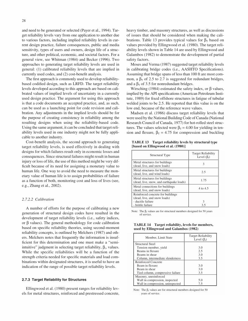
28
and need to be generated or selected (Payer et al., 1994). Tar-get reliability levels vary from one application to another dueto various factors, including implied reliability levels in cur-rent design practice, failure consequences, public and mediasensitivity, types of users and owners, design life of a struc-ture, and other political, economic, and societal factors. For ageneral view, see Whitman (1984) and Becker (1996). Twoapproaches to generating target reliability levels are used ingeneral: (1) calibrated reliability levels that are implied incurrently used codes, and (2) cost-benefit analysis.
The first approach is commonly used to develop reliability-based codified design, such as LRFD. The target reliabilitylevels developed according to this approach are based on cali-brated values of implied levels of uncertainty in a currentlyused design practice. The argument for using this approachis that a code documents an accepted practice, and, as such,can be used as a launching point for code revision and cali-bration. Any adjustments in the implied levels should be forthe purpose of creating consistency in reliability among theresulting designs when using the reliability-based code.Using the same argument, it can be concluded that target reli-ability levels used in one industry might not be fully appli-cable to another industry.
Cost-benefit analysis, the second approach to generatingtarget reliability levels, is used effectively in dealing withdesigns for which failures result only in economic losses andconsequences. Since structural failures might result in humaninjury or loss of life, the use of this method might be very dif-ficult because of its need for assigning a monetary value tohuman life. One way to avoid the need to measure the mon-etary value of human life is to assign probabilities of failureas a function of both, monitoring cost and loss of lives (see,e.g., Zhang et al., 2002).
2.7.2.2 Calibration
A number of efforts for the purpose of calibrating a newgeneration of structural design codes have resulted in thedevelopment of target reliability levels (i.e., safety indices,or β values). The general methodology for code calibrationbased on specific reliability theories, using second-momentreliability concepts, is outlined by Melchers (1987) and oth-ers. Melchers notes that frequently the information is insuf-ficient for this determination and one must make a “semi-intuitive” judgment in selecting target reliability, βt, values.While the specific reliabilities will be a function of thestrength criteria needed for specific materials and load com-binations within designated structures, it is useful to have anindication of the range of possible target reliability levels.
2.7.3 Target Reliability for Structures
Ellingwood et al. (1980) present ranges for reliability lev-els for metal structures, reinforced and prestressed concrete,
heavy timber, and masonry structures, as well as discussionsof issues that should be considered when making the cali-brations. Table 13 provides typical values for βT based onvalues provided by Ellingwood et al. (1980). The target reli-ability levels shown in Table 14 are used by Ellingwood andGalambos (1982) to demonstrate the development of partialsafety factors.
Moses and Verma (1987) suggested target reliability levelsin calibrating bridge codes (i.e., AASHTO Specifications).Assuming that bridge spans of less than 100 ft are most com-mon, a βT of 2.5 to 2.7 is suggested for redundant bridges,and a βT of 3.5 for nonredundant bridges.
Wirsching (1984) estimated the safety index, or β values,implied by the API specifications (American Petroleum Insti-tute, 1989) for fixed offshore structures in fatigue of tubularwelded joints to be 2.5. He reported that this value is on thelow end, because of the reference wave values.
Madsen et al. (1986) discuss target reliability levels thatwere used by the National Building Code of Canada (NationalResearch Council of Canada, 1977) for hot-rolled steel struc-tures. The values selected were βT = 4.00 for yielding in ten-sion and flexure, βT = 4.75 for compression and buckling
Structural Type Target Reliability Level (βt)
Metal structures for buildings (dead, live, and snow loads)
3
Metal structures for buildings (dead, live, and wind loads) 2.5
Metal structures for buildings (dead, live, snow, and earthquake loads) 1.75
Metal connections for buildings (dead, live, and snow loads) 4 to 4.5
Reinforced concrete for buildings (dead, live, and snow loads) - ductile failure - brittle failure
3 3.5
Note: The βt values are for structural members designed for 50 years of service.
Member, Limit State Target Reliability Level (βt)
Structural Steel Tension member, yield Beams in flexure Beams in shear Column, intermediate slenderness
3.0 2.5 3.0 3.5
Reinforced Concrete Beam in flexure Beam in shear Tied column, compressive failure
3.0 3.0 3.5
Masonry, unreinforced Wall in compression, inspected Wall in compression, uninspected
5.0 7.5
Note: The βt values are for structural members designed for 50 years of service.
TABLE 14 Target reliability, levels for members,used by Ellingwood and Galambos (1982)
TABLE 13 Target reliability levels by structural type[based on Ellingwood et al. (1980)]

29
failure, and βT = 4.25 for shear failures. These values arehigher than those in Tables 13 and 14 because they reflect dif-ferent environmental loading conditions and, possibly, differ-ent design life. The Canadian Standard Association presentedthe following target failure probabilities for developingdesign criteria for offshore installation in Canadian waters(Mansour et al., 1994): 10−5 per year for failures that wouldresult in great loss of life or have a high potential for envi-ronmental damage; and 10−3 per year for failures that resultin small risk to life or a low potential for environmental dam-age. (It is important to note that no direct relationship existsbetween general probability of failure and annual probabilityof failure.)
Madsen et al. (1986) also discuss target reliability levelsthat were used by the Nordic Committee on Building Regu-lations (1978). Target reliability values were selecteddepending on the failure consequences of a building: βT = 3.1for less serious failure consequences, βT = 5.2 for very seri-ous failure consequences, and βT = 4.3 for common cases.
2.7.4 Geotechnical Perspective
The review provided in section 2.7.3 suggests that typicaltarget reliability for members and structures relevant to bridgeconstruction varies between 1.75 and 3.0, with a target relia-bility of 2.5 to 2.7 for relevant bridges.
Barker et al. (1991, p. A-51) state the following regardingtarget reliability index for driven piles:
Meyerhof (1970) showed that the probability of failure offoundations should be between 10−3 and 10−4, which corre-sponds to values of β between 3 and 3.6. The reliability indexof offshore piles reported by Wu, et al. (1989) is between 2and 3. They calculated that the reliability index for pile sys-tems is somewhat higher and is approximately 4.0, corre-sponding to a lifetime probability of failure of 0.00005. Tanget al. (1990) reported that offshore piles have a reliabilityindex ranging from 1.4 to 3.0.
Reliability indices for driven piles are summarized in Table5.4 [Table 15 of this report]. Values of β between 1.5 and 2.8are generally obtained for the lognormal procedure. Thus atarget value of β between 2.5 to 3 may be appropriate. How-ever, piles are usually used in groups. Failure of one pile doesnot necessarily imply that the pile group will fail. Because ofthis redundancy in pile groups, it is felt that the target relia-bility index for driven piles can be reduced from 2.5 to 3.0 toa value between 2.0 and 2.5.
Zhang et al. (2001) used a first order reliability method toevaluate the reliability of axially loaded pile groups designedusing the traditional concept of group efficiency. Group effectsand system effects were identified as the major causes of thesignificantly greater observed reliability of pile foundationscompared to the calculated reliability of single piles. Groupeffect relates to the combined action of any number of pilesvs. a single pile. A system effect is the contribution of thesuperstructure stiffness to the load distribution and resistance.
The calculated probability of failure of pile groups wasfound to be 1 to 4 orders of magnitude smaller than that ofsingle piles, depending on the significance of system effects(changing the system bias factor λs from 1 to 2). Based ontheir study, Zhang et al. (2001) state that the target reliabil-ity index, βT, for achieving a specified reliability level shoulddiffer for an isolated single pile (β), an isolated pile group(βTG), and a pile system (βTS). They give the following rec-ommendations based on their research:
1. A βTG value of 3.0 requires a β of 2.0 to 2.8 if no sys-tem effects are considered.
2. A βTG value of 3.0 requires a β of 1.7 to 2.5 if a systemeffect factor of 1.5 is considered.
Additional aspect to the increased reliability of deep foun-dations can be obtained from the limited data availableregarding the loads, which actually arrive at the piles duringtheir service. Tang et al. (1994) followed the response ofdrilled shafts during construction loading and found that,while 44% to 67% of the design load was measured at thepile’s top, only 6% to 13% of the design load arrived at thetip in the rock socket. In the design of drilled shafts the fric-tion or the end bearing are often being neglected, especiallyin rock sockets. This practice and the observed values sug-gest that piles are often underutilized (over conservative), afact contributing to the reliability of pile foundations, whichrarely fail. These facts, while recognized, cannot be consid-ered when assigning a target reliability value until more dataare available and relevant load factors can be directly devel-oped for foundations.
2.7.5 Recommended Target Reliability
2.7.5.1 General Range for Single Piles and Pile Groups
Based on the above review and the data presented, it seemsreasonable to establish the target reliability between 2.0 and2.5 for pile groups and as high as 3.0 for single piles.
It is clear from the review that, while the redundancy ofpile groups serves as the major reason for the decrease in tar-get reliability, no logical distinction was made (when choos-ing target reliability) between the target reliability of singlepiles and pile groups. One can evaluate the performance ofthe piles on the basis of their “redundancy.” A nonredundant
Reliability Index, β Dead to Live Load Ratio Lognormal Advanced
1.00 1.6 – 2.8 1.6 – 3.0 3.69 1.7 – 3.1 1.8 – 3.3
TABLE 15 Reliability indices for driven piles(Barker et al., 1991)

30
member is one for which failure will directly affect the ele-ment carried by it (i.e., the column) with limited or no abilityof other foundations supporting the same element to mitigatethe effect of the failure of the member. Referring to Figure 13,one can intuitively see that, as three points define a plane, afailure of any deep foundation element in such a configura-tion cannot be mitigated by the others. Though details of thefoundation scheme are important—see, e.g., FoundationDesign Standards in the World (Japanese Geotechnical Soci-ety, 1998)—one can distinguish between a 5-member scheme(clearly redundant) and a 3- or fewer member scheme (non-redundant) for the purpose of establishing a target reliability.
The evaluation of the resistance factors in the presentstudy was originally carried out by using reliability indicesof 2.0, 2.5, and 3.0 associated with pf = 2.28%, 0.62%, and0.14%, respectively. This approach provided a reasonablerange of values to investigate before the final target reliabil-ity values were set.
2.7.5.2 Recommended Concept and Targets
Based on the review of the state of the art, the survey ofcommon practice, and the evaluation of the above values, thefollowing reliability indices and probability of failure weredeveloped and are recommended in conjunction with meth-ods for capacity evaluation of single piles (see Figure 13):
1. For redundant piles, defined as 5 or more piles per pilecap, the recommended probability of failure is pf = 1%,corresponding to a target reliability index of β = 2.33.
2. For nonredundant piles, defined as 4 or fewer piles perpile cap, the recommended probability of failure is pf =0.1%, corresponding to a reliability index of β = 3.00.
2.8 INVESTIGATION OF THE RESISTANCE FACTORS
2.8.1 Initial Resistance Factors Calculations
The factors were evaluated using FORM (First Order Reli-ability Method) with dead load (DL) to live load (LL) ratiosranging from 1 to 4. The results for a bias of one and a coef-
ficient of variation of 0.4 and target reliability values of 2.0,2.5, and 3.0 presented in Figure 14, suggest very little sensi-tivity of the resistance factors to the DL to LL ratio. A simi-lar trend was observed using DL to LL ratio of 10. The largedead-to-live-load ratios represent conditions of bridge con-struction, typically associated with very long bridge spans.The relatively small influence of the dead-to-live-load ratioon the calculated resistance factors suggests that (1) the useof a DL to LL ratio of 2 or 2.5 as a typical value is reason-able, and (2) the obtained factors are, by and large, applica-ble for long span bridges.
2.8.2 Parameter Study—The Limited Meaningof the Resistance Factor Value
The use of FORM requires an iterative process and hencea parametric study more easily obtained by using the FOSMrelationships, assuming the results of both are within a closerange (to be demonstrated in section 3.2.2). Figure 15 pre-sents such relations using Equation 10, the chosen load dis-tribution parameters (Equations 25 and 26), DL to LL ratio of2.5 and a target reliability β = 2.33 (see section 2.7.5.2). Theobtained relationship shows that a perfect prediction (λ = 1,COV = 0) would result with a resistance factor of (φ = 0.80.With a prediction method for which the bias is one but thedistribution is greater (COV > 0), the resistance factor wouldsharply decrease so that for COV = 0.4 the resistance factorwould reduce to φ = 0.44. The influence of the bias of themethod (λ, or mean ratio of measured over predicted) on theresistance factor is equally important. As seen in the figure,an under predictive method (λ > 1) has a “built in” safety andhence a higher resistance factor is used in order to achievethe same target reliability as would be obtained by using amethod which predicts, on average, more accurately (λ ≈ 1).For example, for methods having the same distribution(COV = 0.4), an underpredictive method with a bias of λ =1.5 would result in a resistance factor φ = 0.67, whereas amethod with a bias λ = 1.0 would result in φ = 0.44. Although
Redundant Non - Redundant
Logically Non-Redundant
β β β β = 2.33 Pf = 1.0%ββββ = 3.00 Pf = 0.1%
0 1 2 3 4 5DL/LL - Dead to Live Load Ratio
0.4
0.6
0.8
Res
ista
nce
Fac
tor,
φ
General CaseBias = 1 COV = 0.4
β = 2.0Pf= 2.28%
β = 2.5pf= 0.62%
β = 3.0Pf= 0.14%
Figure 13. Redundant vs. non-redundant pile supportand the current research recommendations of targetreliability.
Figure 14. Calculated resistance factors for a generalcase showing the influence of the dead-to-live-load ratio.
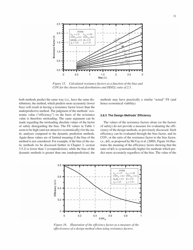
31
both methods predict the same way (i.e., have the same dis-tribution), the method, which predicts more accurately (lowerbias) will result in having a resistance factor lower than theunderpredictive method. The judgment of the methods’ eco-nomic value (“efficiency”) on the basis of the resistancevalue is therefore misleading. The same argument can bemade regarding the misleading absolute values of the factorof safety disregarding the bias. The FS values in Table 1seem to be high (and not attractive economically) for the sta-tic analyses compared to the dynamic prediction methods.Again these values are of limited meaning if the bias of themethod is not considered. For example, if the bias of the sta-tic methods (to be discussed further in Chapter 3, section3.5.2) is lower than 1 (overprediction), while the bias of thedynamic methods is greater than one (underprediction), the
methods may have practically a similar “actual” FS (andhence economical viability).
2.8.3 The Design Methods’ Efficiency
The values of the resistance factors alone (or the factorsof safety) do not provide a measure for evaluating the effi-ciency of the design methods, as previously discussed. Suchefficiency can be evaluated through the bias factor, and itsCOV, or the ratio of the resistance factor to the bias factor,i.e., φ/λ, as proposed by McVay et al. (2000). Figure 16 illus-trates the meaning of the efficiency factor showing that theratio of φ/λ is systematically higher for methods which pre-dict more accurately regardless of the bias. The value of the
0 0.5 1 1.5 2 2.5 3Bias (λ)
0.0
0.5
1.0
1.5
2.0
2.5
Res
ista
nce
Fac
tor
(φ)
FOSMλQL = 1.15 λQD = 1.05COVQL= 0.2 COVQD =0.1
QD/QL = 2.5 β = 2.33γD = 1.25, γL = 1.75
COV = 0
0.2
0.4
0.6
0.8
0.5
COV = 1.00
Figure 15. Calculated resistance factors as a function of the bias andCOV for the chosen load distributions and DD/LL ratio of 2.5.
0 0.2 0.4 0.6 0.8 1COVR
0
0.2
0.4
0.6
0.8
Eff
icie
ncy
(φ/λ
)
FOSMλQL = 1.15 λQD = 1.05COVQL = 0.2 COVQD = 0.1
QD/QL = 2.5 β = 2.33
γD = 1.25 γL = 1.75
Figure 16. Illustration of the efficiency factor as a measure of theeffectiveness of a design method when using resistance factors.

32
efficiency factor remains constant for all bias combinationsfor a given COV, leading to higher values for methods with alower COV. Using the example given in section 2.8.2, amethod with COV = 0.4, λ = 1.0, and φ = 0.44 will result inφ/λ = 0.44; a second method with COV = 0.4, λ = 1.5, and φ =0.67 will result in the same φ/λ = 0.44. Thus, although onemethod presents a resistance factor of 0.67 and the other of0.44, both methods have identical efficiency and should resultin identical design; hence they have the same economic value.The efficiency of a given capacity prediction method can,therefore, be improved only through a reduction in its vari-
ability (COV); alternatively, design methods need to be cho-sen based on their COV.
This measure of efficiency needs to accompany prescribedresistance factors in order to avoid a misconception of theexistence of a correlation between the economy of a designmethod and high resistance factors when compared to others.Similarly, such misconceptions exist between the economicvalue of a method and the lower level of a factor of safety,where a mean factor of safety (defined as FS x bias) repre-sents the economic value of the method (the lower the bet-ter), as proposed by Paikowsky et al. (1994).

33
CHAPTER 3
INTERPRETATION, APPRAISAL, AND APPLICATIONS
3.1 ANALYSIS RESULTS AND RESISTANCE FACTORS
3.1.1 Driven Piles—Static Analysis
Table 16 presents a summary of the results obtained fromthe analyses used for static capacity evaluation of driven piles,compared with the nominal resistance based on Davisson’sfailure criterion. The information is grouped by soil and piletype and design method. The table includes statistical param-eters and resistance factors for a range of reliability indexvalues, and a ratio of DL to LL of 2.0.
The data leading to Table 16 were statistically analyzed toremove outliers (i.e., extreme cases; Section 3.5 provides adiscussion of this process); and the table includes only thosecases within ±2 standard deviations of the mean. As can beseen, subcategorization based on pile or soil type may resultin subsets too small for reasonable statistical analysis. On theother hand, many of the subsets have similar statistics andresistance factors and hence can be combined. It is importantto note that many common design methods for all piles in allsoils overpredict the actual (i.e., measured) pile-capacity.This explains the traditional need for high factors of safetyfor static design (e.g., see Table 1).
A more complete picture of the performance of a method isobtained by plotting the histogram of observed to predictedcapacities and overlaying the best-fitting normal and lognor-mal PDFs. Figures 17 through 26 present such plots for theselected cases of static analyses of driven piles. The figuresare arranged in order from the most inclusive logical case, asthe data permit, to subsets of the same category. For example,Figure 17 presents the performance of the α-API method forall pile types (52 cases of H, concrete and pipe piles) in clay.Figures 18 and 19 present the performance of the method forsubsets of concrete (36 cases) and H piles (16 cases),respectively. Additional graphical presentations of the dataare included in Appendix C.
3.1.2 Driven Piles—Dynamic Analysis
3.1.2.1 The Analyzed Cases
Time of driving, driving resistance, and area ratio provedto be controlling parameters for the dynamic methods (sec-
tion 2.5.3). The PD/LT 2000 database was first separated intodesign and construction categories. The dynamic methodsused in construction were subdivided between methods thatuse dynamic measurements and those that do not. These, inturn, were subcategorized according to the controlling param-eters. Figure 27 presents the analyzed subsets, the number ofcase histories in each set, and the mean and standard devia-tion for each.
WEAP is utilized in the design stage. The analysis (notincluded in this research) needs to be carried out for drivingstress evaluation, leading to a load factor. The use of themethod for the evaluation of pile capacity was examinedthrough the comparison of WEAP results for default input val-ues and the blow count at the EOD with static load test results.The data presented were provided by GRL Inc. (Hanniganet al., 1996).
For the construction category, the dynamic analyses meth-ods without dynamic measurements are the ENR, Gates,and FHWA version of Gates. The methods with dynamicmeasurements are CAPWAP and the Energy Approach. Thedynamic methods are broken down into subsets based on timeof driving, driving resistance, and area ratios. Judgment andstatistical guidelines were used for the inclusion or exclusionof cases. For example, extreme CAPWAP underpredictions(beyond 2 standard deviations) were observed at EOD at onesite. All the case histories on that site included easy drivingand large area ratios; if included in the general population ofthe data, the EOD statistics would have become 1.861 ± 1.483(mean ± 1 S.D.). This site is included only in the subcategoryof blow count < 16 BP10cm and AR < 350.
3.1.2.2 The Critical Categories
The outcomes of the statistical analyses presented in Figure27 allow the identification of critical categories that requirecalibration and development into resistance factors. For exam-ple, the critical CAPWAP cases include (1) all data, (2) EOD,(3) BOR, and (4) the worst combination of soil motion effect(Blow count < 16 BP10cm and AR < 350). Table 17 presents asummary of the major categories of the dynamic methodsidentified from Figure 27 as those that require calibration fora resistance factor.

34
Resistance Factors for a Given
Reliability Index ββββ Soil
Type Pile
Type N Design Method(1) Details of Method(2)
Application Mean
Stand. Dev.
COV
2.00 2.50 3.00
4 β-Method 11.5 B; T&P(2) 0.61 0.37 0.61 0.23 0.18 0.13
16 λ-Method 11.5B; T&P(2) 2B; T&P(5) 0.74 0.29 0.39 0.43 0.35 0.29
17 α-Tomlinson 2B; T&P(2) 0.82 0.33 0.40 0.46 0.38 0.31
16 α-API 2B; T&P(5) 0.90 0.37 0.41 0.50 0.41 0.33
H-Piles
8 SPT-97 mob 1.04 0.43 0.41 0.57 0.47 0.38
18 λ-Method 2B; Hara (5h) 0.76 0.22 0.29 0.53 0.45 0.38
17 α-API 2B; Hara (5h) 0.81 0.21 0.26 0.60 0.52 0.44
8 β-Method 2B; Hara (5h) 0.81 0.41 0.51 0.37 0.30 0.23 Concrete
Piles
18 α-Tomlinson 2B; Hara (5h) 0.87 0.42 0.48 0.42 0.34 0.26
18 α-Tomlinson 2B; T&P (1) 0.64 0.32 0.50 0.30 0.24 0.19
19 α-API 2B; T&P (1) 0.79 0.43 0.54 0.34 0.27 0.20
12 β-Method 2B; T&P (1) 0.45 0.27 0.60 0.17 0.13 0.10
19 λ-Method 2B; T&P (1) 0.67 0.37 0.55 0.28 0.22 0.17
Clay
Pipe Piles
12 SP T-97 mob 2B; T&P (1) 0.39 0.24 0.62 0.15 0.11 0.08
19 Nordlund 36; 11.5B,P(6) 0.94 0.38 0.40 0.53 0.43 0.35
18 Meyerhof 0.81 0.31 0.38 0.47 0.39 0.32
19 β-Method 36; 2B; P(5) 0.78 0.40 0.51 0.36 0.28 0.22 H-Piles
18 SPT-97 mob 1.35 0.58 0.43 0.72 0.59 0.47
36 Nordlund 36: 11.5B; P(6) 1.02 0.49 0.48 0.50 0.40 0.31
35 β-Method 36; 2B; P(5) 1.10 0.48 0.44 0.58 0.47 0.38
36 Meyerhof 0.61 0.37 0.61 0.23 0.18 0.13Concrete
Piles
36 SPT-97 mob 1.21 0.57 0.47 0.60 0.48 0.38
19 Nordlund 36; 2B P(5) 1.48 0.77 0.52 0.67 0.52 0.41
20 β-Method 36; 2B P(5) 1.18 0.73 0.62 0.44 0.33 0.25
20 Meyerhof 0.94 0.55 0.59 0.37 0.29 0.22
Sand
Pipe Piles
19 SPT-97 mob 1.58 0.82 0.52 0.71 0.56 0.44
20 α-Tomlinson/Nordlund/Thurman 36; 2B; P(5) 0.59 0.23 0.39 0.34 0.28 0.23
34 α-API/Nordlund/Thurman 36; 2B; P(5) 0.79 0.35 0.44 0.41 0.33 0.27
32 β-Method/Thurman 36; 2B; P(5) 0.48 0.23 0.48 0.23 0.19 0.15 H-Piles
40 SP T-97 1.23 0.55 0.45 0.64 0.51 0.41
33 α-Tomlinson/Nordlund/Thurman 36; 2B; P; Hara(5h) 0.96 0.47 0.49 0.46 0.36 0.29
80 α-API/Nordland/Thurman 36; 11.5B; Sch; T&P(8) 0.87 0.42 0.48 0.42 0.34 0.26
80 β-Method/Thurman 36; 11.5B; Sch; T&P(8) 0.81 0.31 0.38 0.47 0.39 0.32
71 SPT-97 mob 1.81 0.91 0.50 0.84 0.67 0.52
Concrete Piles
30 FHWA CPT 0.84 0.26 0.31 0.57 0.48 0.40
13 α-Tomlinson/Nordlund/Thurman 36; 2B; P(5) 0.74 0.44 0.59 0.29 0.22 0.17
32 α-API/Nordland/Thurman 36; 2B; P(5) 0.80 0.36 0.45 0.41 0.33 0.26
29 β-Method/Thurman 36; 2B; P(5) 0.54 0.26 0.48 0.26 0.21 0.16
Mixed Soils
Pipe Piles
33 SPT-97 mob 0.76 0.29 0.38 0.45 0.37 0.30
(1)See Table 6 for details; (2) Numbers in parentheses refer to notations used for detailing soil parameters combinations (see Table 7b and Appendix C for more details),
See Tables 7a and 8 for soil properties’ correlations to SPT and CPT respectively, 36 = limiting friction angle, B = pile diameter 2B, 11.5B contributing zone to tip resistance.
TABLE 16 The performance of the driven piles’ static analysis methods—statistical summary and resistance factors for data using mean ± 2 SD
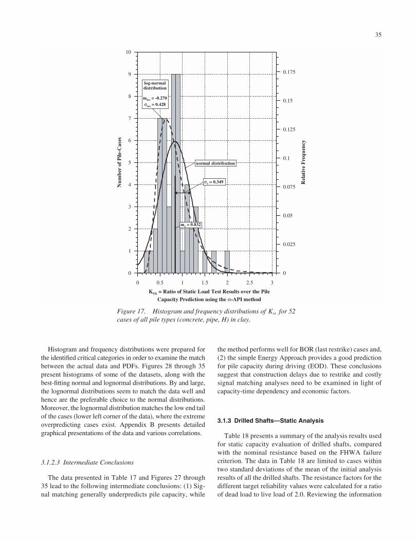
Histogram and frequency distributions were prepared forthe identified critical categories in order to examine the matchbetween the actual data and PDFs. Figures 28 through 35present histograms of some of the datasets, along with thebest-fitting normal and lognormal distributions. By and large,the lognormal distributions seem to match the data well andhence are the preferable choice to the normal distributions.Moreover, the lognormal distribution matches the low end tailof the cases (lower left corner of the data), where the extremeoverpredicting cases exist. Appendix B presents detailedgraphical presentations of the data and various correlations.
3.1.2.3 Intermediate Conclusions
The data presented in Table 17 and Figures 27 through35 lead to the following intermediate conclusions: (1) Sig-nal matching generally underpredicts pile capacity, while
35
the method performs well for BOR (last restrike) cases and,(2) the simple Energy Approach provides a good predictionfor pile capacity during driving (EOD). These conclusionssuggest that construction delays due to restrike and costlysignal matching analyses need to be examined in light ofcapacity-time dependency and economic factors.
3.1.3 Drilled Shafts—Static Analysis
Table 18 presents a summary of the analysis results usedfor static capacity evaluation of drilled shafts, comparedwith the nominal resistance based on the FHWA failure criterion. The data in Table 18 are limited to cases within two standard deviations of the mean of the initial analysisresults of all the drilled shafts. The resistance factors for thedifferent target reliability values were calculated for a ratioof dead load to live load of 2.0. Reviewing the information
0 0.5 1 1.5 2 2.5 3
KSX = Ratio of Static Load Test Results over the PileCapacity Prediction using the α-API method
0
1
2
3
4
5
6
7
8
9
10
Nu
mb
er o
f P
ile-C
ases
0
0.025
0.05
0.075
0.1
0.125
0.15
0.175
Rel
ativ
e F
req
uen
cy
log-normaldistribution
mlnx = -0.270σlnx = 0.428
normal distribution
mx = 0.832
σx = 0.349
Figure 17. Histogram and frequency distributions of Ksx for 52cases of all pile types (concrete, pipe, H) in clay.
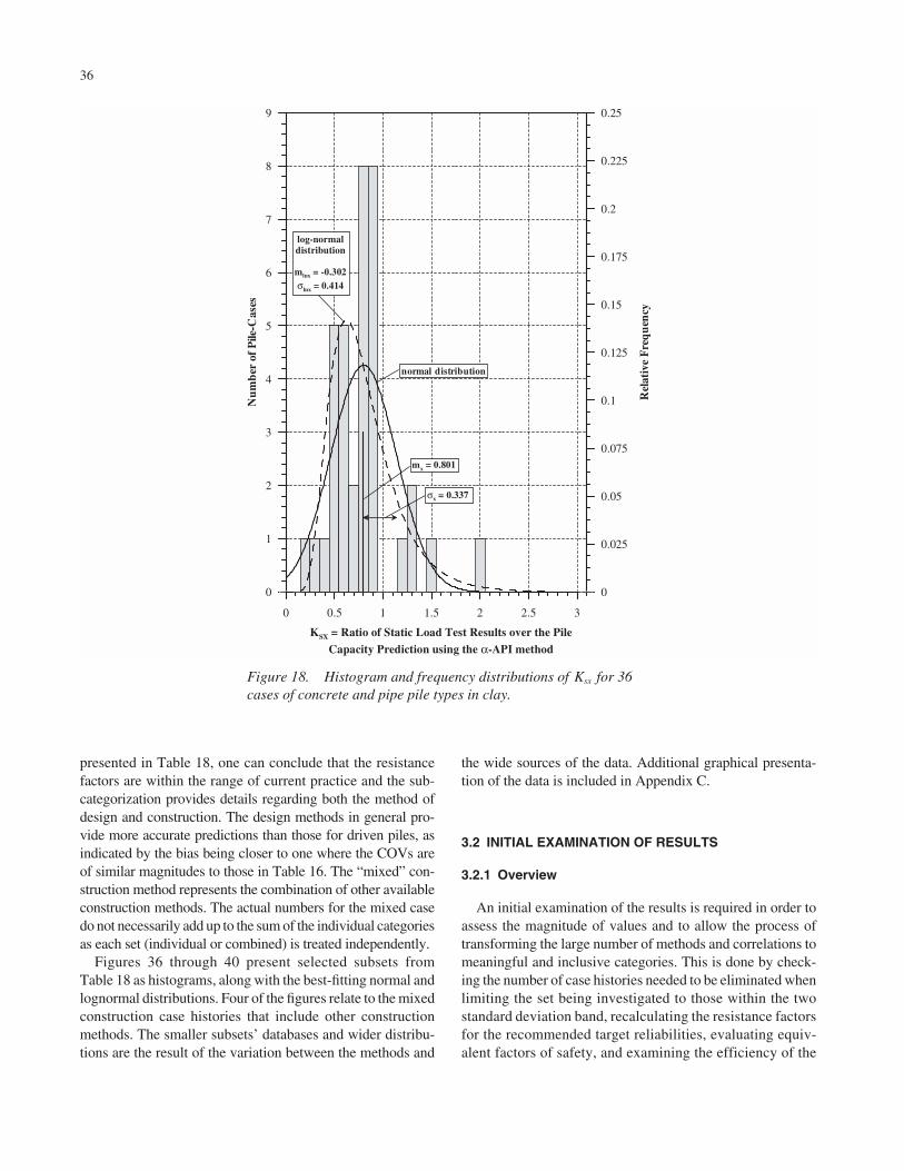
presented in Table 18, one can conclude that the resistancefactors are within the range of current practice and the sub-categorization provides details regarding both the method ofdesign and construction. The design methods in general pro-vide more accurate predictions than those for driven piles, asindicated by the bias being closer to one where the COVs areof similar magnitudes to those in Table 16. The “mixed” con-struction method represents the combination of other availableconstruction methods. The actual numbers for the mixed casedo not necessarily add up to the sum of the individual categoriesas each set (individual or combined) is treated independently.
Figures 36 through 40 present selected subsets fromTable 18 as histograms, along with the best-fitting normal andlognormal distributions. Four of the figures relate to the mixedconstruction case histories that include other constructionmethods. The smaller subsets’ databases and wider distribu-tions are the result of the variation between the methods and
36
the wide sources of the data. Additional graphical presenta-tion of the data is included in Appendix C.
3.2 INITIAL EXAMINATION OF RESULTS
3.2.1 Overview
An initial examination of the results is required in order toassess the magnitude of values and to allow the process oftransforming the large number of methods and correlations tomeaningful and inclusive categories. This is done by check-ing the number of case histories needed to be eliminated whenlimiting the set being investigated to those within the twostandard deviation band, recalculating the resistance factorsfor the recommended target reliabilities, evaluating equiv-alent factors of safety, and examining the efficiency of the
Figure 18. Histogram and frequency distributions of Ksx for 36cases of concrete and pipe pile types in clay.
0 0.5 1 1.5 2 2.5 3
KSX = Ratio of Static Load Test Results over the PileCapacity Prediction using the α-API method
0
1
2
3
4
5
6
7
8
9
Nu
mb
er o
f P
ile-C
ases
0
0.025
0.05
0.075
0.1
0.125
0.15
0.175
0.2
0.225
0.25
Rel
ativ
e F
req
uen
cy
log-normaldistribution
mlnx = -0.302σlnx = 0.414
mx = 0.801
σx = 0.337
normal distribution
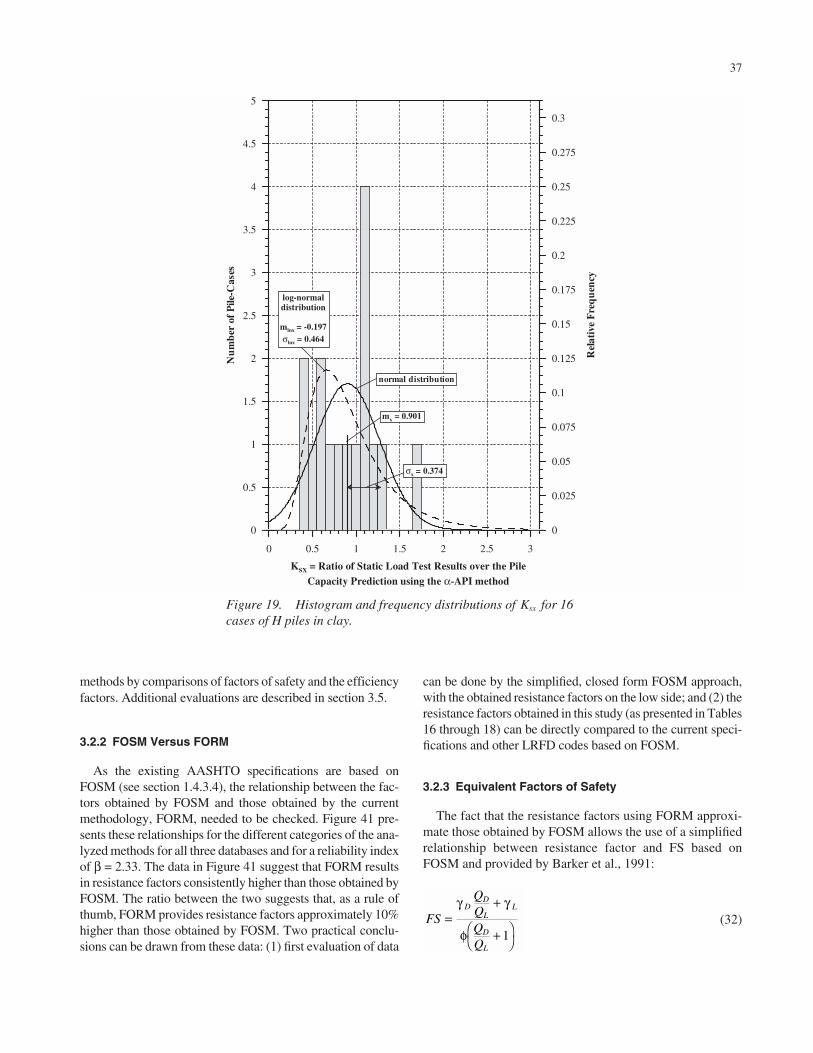
methods by comparisons of factors of safety and the efficiencyfactors. Additional evaluations are described in section 3.5.
3.2.2 FOSM Versus FORM
As the existing AASHTO specifications are based onFOSM (see section 1.4.3.4), the relationship between the fac-tors obtained by FOSM and those obtained by the currentmethodology, FORM, needed to be checked. Figure 41 pre-sents these relationships for the different categories of the ana-lyzed methods for all three databases and for a reliability indexof β = 2.33. The data in Figure 41 suggest that FORM resultsin resistance factors consistently higher than those obtained byFOSM. The ratio between the two suggests that, as a rule ofthumb, FORM provides resistance factors approximately 10%higher than those obtained by FOSM. Two practical conclu-sions can be drawn from these data: (1) first evaluation of data
37
can be done by the simplified, closed form FOSM approach,with the obtained resistance factors on the low side; and (2) theresistance factors obtained in this study (as presented in Tables16 through 18) can be directly compared to the current speci-fications and other LRFD codes based on FOSM.
3.2.3 Equivalent Factors of Safety
The fact that the resistance factors using FORM approxi-mate those obtained by FOSM allows the use of a simplifiedrelationship between resistance factor and FS based onFOSM and provided by Barker et al., 1991:
(32)FS
QQQQ
DD
LL
D
L
=+
+
γ γ
φ 1
0 0.5 1 1.5 2 2.5 3
KSX = Ratio of Static Load Test Results over the PileCapacity Prediction using the α-API method
0
0.5
1
1.5
2
2.5
3
3.5
4
4.5
5
Nu
mb
er o
f P
ile-C
ases
0
0.025
0.05
0.075
0.1
0.125
0.15
0.175
0.2
0.225
0.25
0.275
0.3
Rel
ativ
e F
req
uen
cy
log-normaldistribution
mlnx = -0.197σlnx = 0.464
mx = 0.901
σx = 0.374
normal distribution
Figure 19. Histogram and frequency distributions of Ksx for 16cases of H piles in clay.
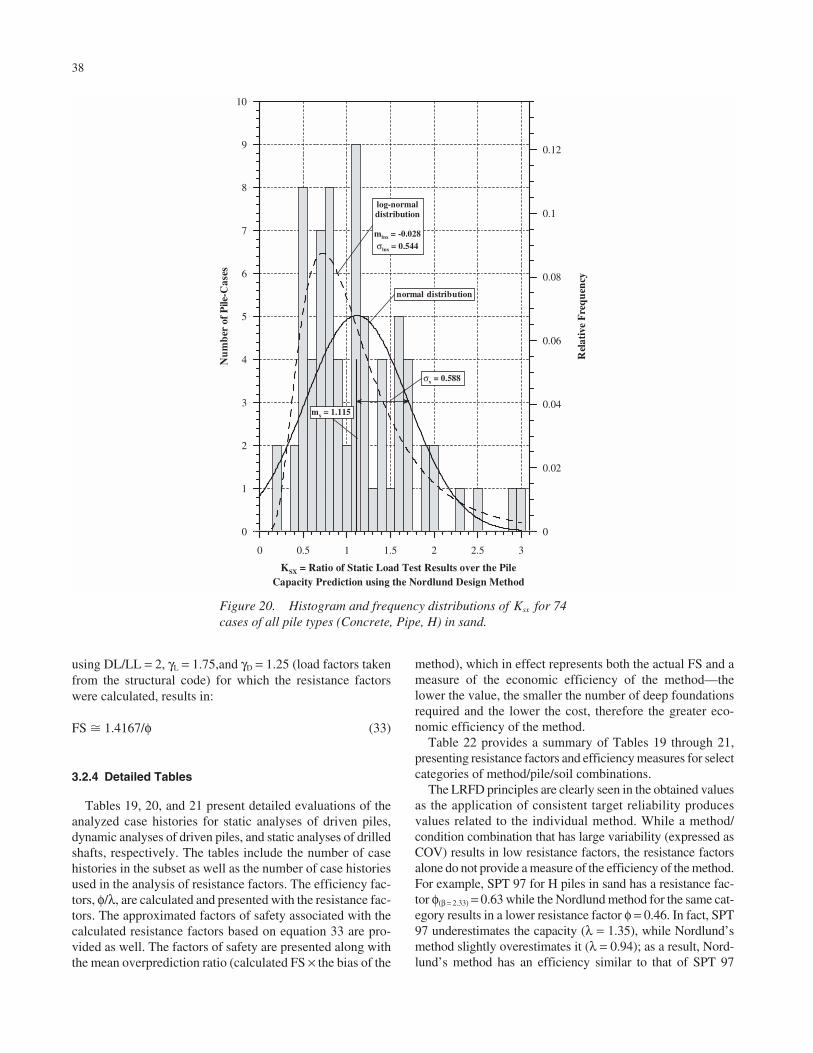
using DL/LL = 2, γL = 1.75,and γD = 1.25 (load factors takenfrom the structural code) for which the resistance factorswere calculated, results in:
FS � 1.4167/φ (33)
3.2.4 Detailed Tables
Tables 19, 20, and 21 present detailed evaluations of theanalyzed case histories for static analyses of driven piles,dynamic analyses of driven piles, and static analyses of drilledshafts, respectively. The tables include the number of casehistories in the subset as well as the number of case historiesused in the analysis of resistance factors. The efficiency fac-tors, φ/λ, are calculated and presented with the resistance fac-tors. The approximated factors of safety associated with thecalculated resistance factors based on equation 33 are pro-vided as well. The factors of safety are presented along withthe mean overprediction ratio (calculated FS × the bias of the
38
method), which in effect represents both the actual FS and ameasure of the economic efficiency of the method—thelower the value, the smaller the number of deep foundationsrequired and the lower the cost, therefore the greater eco-nomic efficiency of the method.
Table 22 provides a summary of Tables 19 through 21,presenting resistance factors and efficiency measures for selectcategories of method/pile/soil combinations.
The LRFD principles are clearly seen in the obtained valuesas the application of consistent target reliability producesvalues related to the individual method. While a method/condition combination that has large variability (expressed asCOV) results in low resistance factors, the resistance factorsalone do not provide a measure of the efficiency of the method.For example, SPT 97 for H piles in sand has a resistance fac-tor φ(β = 2.33) = 0.63 while the Nordlund method for the same cat-egory results in a lower resistance factor φ = 0.46. In fact, SPT97 underestimates the capacity (λ = 1.35), while Nordlund’smethod slightly overestimates it (λ = 0.94); as a result, Nord-lund’s method has an efficiency similar to that of SPT 97
0 0.5 1 1.5 2 2.5 3
KSX = Ratio of Static Load Test Results over the PileCapacity Prediction using the Nordlund Design Method
0
1
2
3
4
5
6
7
8
9
10
Nu
mb
er o
f P
ile-C
ases
0
0.02
0.04
0.06
0.08
0.1
0.12
Rel
ativ
e F
req
uen
cy
log-normaldistribution
mlnx = -0.028σlnx = 0.544
mx = 1.115
σx = 0.588
normal distribution
Figure 20. Histogram and frequency distributions of Ksx for 74cases of all pile types (Concrete, Pipe, H) in sand.
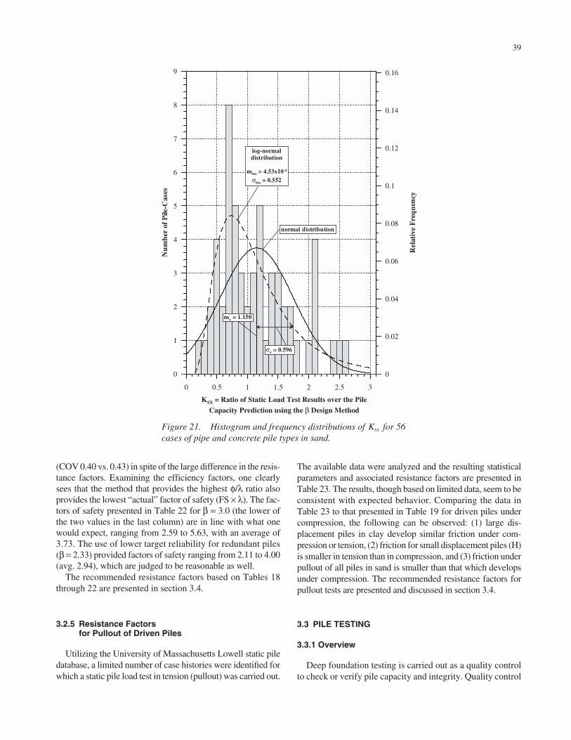
(COV 0.40 vs. 0.43) in spite of the large difference in the resis-tance factors. Examining the efficiency factors, one clearlysees that the method that provides the highest φ/λ ratio alsoprovides the lowest “actual” factor of safety (FS × λ). The fac-tors of safety presented in Table 22 for β = 3.0 (the lower ofthe two values in the last column) are in line with what onewould expect, ranging from 2.59 to 5.63, with an average of3.73. The use of lower target reliability for redundant piles(β = 2.33) provided factors of safety ranging from 2.11 to 4.00(avg. 2.94), which are judged to be reasonable as well.
The recommended resistance factors based on Tables 18through 22 are presented in section 3.4.
3.2.5 Resistance Factors for Pullout of Driven Piles
Utilizing the University of Massachusetts Lowell static piledatabase, a limited number of case histories were identified forwhich a static pile load test in tension (pullout) was carried out.
39
The available data were analyzed and the resulting statisticalparameters and associated resistance factors are presented inTable 23. The results, though based on limited data, seem to beconsistent with expected behavior. Comparing the data inTable 23 to that presented in Table 19 for driven piles undercompression, the following can be observed: (1) large dis-placement piles in clay develop similar friction under com-pression or tension, (2) friction for small displacement piles (H)is smaller in tension than in compression, and (3) friction underpullout of all piles in sand is smaller than that which developsunder compression. The recommended resistance factors forpullout tests are presented and discussed in section 3.4.
3.3 PILE TESTING
3.3.1 Overview
Deep foundation testing is carried out as a quality controlto check or verify pile capacity and integrity. Quality control
0 0.5 1 1.5 2 2.5 3
KSX = Ratio of Static Load Test Results over the PileCapacity Prediction using the β Design Method
0
1
2
3
4
5
6
7
8
9
Nu
mb
er o
f P
ile-C
ases
0
0.02
0.04
0.06
0.08
0.1
0.12
0.14
0.16
Rel
ativ
e F
req
uen
cy
log-normaldistribution
mlnx = 4.53x10⁻⁴
σlnx = 0.552
mx = 1.150
σx = 0.596
normal distribution
Figure 21. Histogram and frequency distributions of Ksx for 56cases of pipe and concrete pile types in sand.
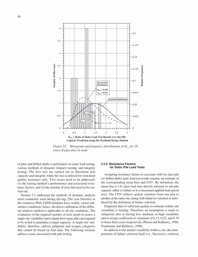
of piles and drilled shafts is performed via static load testing,various methods of dynamic (impact) testing, and integritytesting. The first two are carried out to determine pilecapacity and integrity while the last is utilized for structuralquality assurance only. Two issues need to be addressed:(1) the testing method’s performance and associated resis-tance factors, and (2) the number of tests that need to be car-ried out.
Section 3.1 addressed the methods of dynamic analysismost commonly used during driving. The case histories inthe extensive PD/LT2000 database have widely varied sub-surface conditions; hence, the direct calibration of the differ-ent analysis method is applicable to all site conditions. Theevaluation of the required number of tests needs to assess asingle site variability and evaluate how many piles are requiredto be tested to guarantee a target capacity. A single site vari-ability, therefore, utilizes judgment and assigns categoriesthat cannot be based on firm data. The following sectionsaddress issues associated with pile testing.
40
3.3.2 Resistance Factors for Static Pile Load Tests
Assigning resistance factors to associate with (in situ) pile(or drilled shaft) static load test results requires an estimate ofthe corresponding mean bias and COV. By definition, themean bias is 1.0, since load tests directly measure in situ pilecapacity either to failure or to a maximum applied load (prooftest). The COV reflects spatial variation from one pile toanother at the same site, along with whatever variation is intro-duced by the definition of failure criterion.
Empirical data of sufficient quality to estimate within-sitevariability is lacking. Therefore, an assumption is made tocategorize sites as having low, medium, or high variabilityand to assign coefficient of variations of 0.15, 0.25, and 0.35to these three cases respectively (Phoon and Kulhawy, 1996;Trautmann and Kulhawy, 1996).
In addition to the natural variability within a site, the inter-pretation of failure criterion itself (i.e., Davisson’s criterion
0 0.5 1 1.5 2 2.5 3
KSX = Ratio of Static Load Test Results over the Pile Capacity Prediction using the Nordlund Design Method
0
0.5
1
1.5
2
2.5
3
3.5
4
Nu
mb
er o
f P
ile-C
ases
0
0.025
0.05
0.075
0.1
0.125
0.15
0.175
0.2
Rel
ativ
e F
req
uen
cy
log-normaldistribution
mlnx = 0.250σlnx = 0.561
mx = 1.475
σx = 0.771
normal distribution
Figure 22. Histogram and frequency distributions of Ksx for 19cases of pipe piles in sand.

for driven piles and FHWA for drilled shafts) introducesvariability. Analyses reported in sections 2.3.2 and 2.3.4 suggest that this COV due to the failure criterion alone isabout 0.10. Adding this to the COV for the natural within-site variability yields COVs of 0.18, 0.27, and 0.36 for low,medium, and high variability sites, respectively.
The reduction in COV on the mean pile capacity at thesite should decrease in proportion to 1/√n, where n is thenumber of pile tests (Benjamin and Cornell, 1970). Thisleads to the results presented in Table 24, which describesthe resistance factors as a function of the site variability,number of piles tested, and target reliability. The recom-mended factors assigned are presented in section 3.45.
3.3.3 Numbers of Dynamic Tests Performed on Production Piles
Dynamic pile testing is carried out for quality control, tar-get capacity, integrity, and driving system performance. A
41
certain number of production piles are tested to ensure thatthe piles, as constructed, are satisfactory, in a way that is sim-ilar to quality assurance testing in manufacturing.
For specifying a quality assurance testing plan, the numberof piles to be dynamically tested and the criterion for accept-ing a set of piles need to be determined. Two concerns are atissue: the chance that poor quality (i.e., under capacity) pilesare incorrectly accepted as being good, and the chance thatgood quality piles are incorrectly rejected as being poor (seeFigure 42). For a given level of sampling effort or cost, reduc-ing the chance of one kind of error invariably increases thechance of the other, and thus the two must be balanced.
The definition of “poor quality” piles was taken to be thatthe average pile capacity is less than the design capacity, thatis, less than the reciprocal of the factor of safety. The proba-bility chosen as a reasonable chance that such a set of poorquality piles be incorrectly accepted as good was equilibratedto a reliability index of three, or a probability of about 0.001.This is sometimes called the “buyer’s risk” or the “owner’srisk” as demonstrated in Figures 42 and 43. The definition of
0 0.5 1 1.5 2 2.5 3
KSX = Ratio of Static Load Test Results over the Pile CapacityPrediction using the β Design Method
0
0.5
1
1.5
2
2.5
3
3.5
4
4.5
5
Nu
mb
er o
f P
ile-C
ases
0
0.025
0.05
0.075
0.1
0.125
0.15
0.175
0.2
0.225
0.25
Rel
ativ
e F
req
uen
cy
log-normaldistribution
mlnx = -0.357σlnx = 0.479
mx = 0.783
σx = 0.395
normal distribution
Figure 23. Histogram and frequency distributions of Ksx for 19cases of H piles in sand.

“good quality” piles was taken to be nominal capacity. Theprobability chosen as a reasonable chance that such a set ofgood quality piles be incorrectly rejected as poor was takento be 0.10. This is sometimes called the “seller’s risk” or the“contractor’s risk.”
Given a large total number of piles, N, relative to the num-ber tested, n, the variance of the sample mean, x̄ , is (Benjaminand Cornell, 1970),
(34)
For sampling fractions, f = n/N, greater than about 10%, the“finite population correction factor,” (N − n)/(N − 1), comesinto play. This reduces the sampling variance, because theassumption of sampling without replacement is no longerreasonable. For example, if 100% of the piles are tested, that
Var x N nN
xn
in
i( ) ≅ −− −
=∑1 1
1
42
is, if f = n/N = 1, then there is no variance in the sample aver-age since all the piles have been accounted for.
An assumption, consistent with that projected in section3.3.2, is made to categorize sites as having low, medium, orhigh variability and to assign COVs of 0.15, 0.25, and 0.35to these three cases, respectively. In addition, the dynamictest method also introduces variability. For that, two meth-ods are considered based on the results presented in sections3.1.2 and 3.2.4, Energy Approach (EA) to be used for capac-ity evaluation at the EOD and signal matching (CAPWAP)to be used during BOR.
Setting the owner’s and contractor’s risks on the one hand,and the definitions of “good” and “poor” piles on the other, asdefined above, and noting that the sampling variance of theaverage pile capacity of the tested piles decreases in propor-tion to where n is the number of pile tests, values for thenumber of piles to be tested can be estimated. The obtained
1 n,
0 0.5 1 1.5 2 2.5 3
KSX = Ratio of Static Load Test Results over the Pile CapacityPrediction using the α-API/Nordlund/Thurman design method
0
2
4
6
8
10
12
14
16
18
20
22
Nu
mb
er o
f P
ile-C
ases
0
0.02
0.04
0.06
0.08
0.1
0.12
0.14
Rel
ativ
e F
req
uen
cy
log-normaldistribution
mlnx = -0.293σlnx = 0.494
normal distribution
mx = 0.835
σx = 0.387
Figure 24. Histogram and frequency distributions of Ksx for 146cases of all pile types (concrete, pipe, H) in mixed soil.

recommendations based on these estimates are presented insection 3.4.3.
3.3.4 Testing Drilled Shafts for Major Defects
3.3.4.1 Overview
Drilled shafts require in-field casting and are subject todefects (especially when unlined in cohesionless soils). Accep-tance sampling is used to assess whether an adequate major-ity of a set of shafts is free of major defects.
3.3.4.2 Statistical Background
A sample of n from N shafts is tested to identify majordefects. Major defects are defined as any defect that signifi-cantly compromises the ability of the shaft to carry the assigned
43
loads. Each tested shaft is categorized as either “good” or“defective.” If no more than c of the n tested shafts are“defective,” the set of shafts is accepted. The test parameter,c, is usually a small number.
Suppose that the set of N actual shafts includes m shaftswith major defects. The fraction defective is denoted, p =m/N. Among samples of n tested shafts, the frequency distri-bution of the number of defective tested shafts, c, is of thehypergeometric form,
(35)
in which fc (c | n, N, m) is the frequency distribution, c is thenumber of defective test results within the sample, m is thenumber of defectives in the entire set of N shafts, and Ck
q isthe number of combinations of k out of q things.
f c n N mC C
Ccn cN m
cm
nN| , ,( ) = −
−
0 0.5 1 1.5 2 2.5 3
KSX = Ratio of Static Load Test Results over the Pile CapacityPrediction using the α-API/Nordlund/Thurman design method
0
1
2
3
4
5
6
7
8
9
10
11
12
13
14
15
Nu
mb
er o
f P
ile-C
ases
0
0.02
0.04
0.06
0.08
0.1
0.12
0.14
0.16
0.18
Rel
ativ
e F
req
uen
cy
log-normaldistribution
mlnx = -0.260σlnx = 0.502
mx = 0.868
σx = 0.416
normal distribution
Figure 25. Histogram and frequency distributions of Ksx for 80cases of concrete piles in mixed soil.
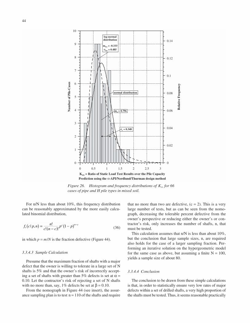
For n/N less than about 10%, this frequency distributioncan be reasonably approximated by the more easily calcu-lated binomial distribution,
(36)
in which p = m /N is the fraction defective (Figure 44).
3.3.4.3 Sample Calculation
Presume that the maximum fraction of shafts with a majordefect that the owner is willing to tolerate in a large set of Nshafts is 5% and that the owner’s risk of incorrectly accept-ing a set of shafts with greater than 5% defects is set at α =0.10. Let the contractor’s risk of rejecting a set of N shaftswith no more than, say, 1% defects be set at β = 0.10.
From the nomograph in Figure 44 (see insert), the assur-ance sampling plan is to test n = 110 of the shafts and require
f c p n nc n c
p pcc n c| , !
! !( ) =
−( ) −( ) −1
44
that no more than two are defective, (c = 2). This is a verylarge number of tests, but as can be seen from the nomo-graph, decreasing the tolerable percent defective from theowner’s perspective or reducing either the owner’s or con-tractor’s risk, only increases the number of shafts, n, thatmust be tested.
This calculation assumes that n/N is less than about 10%,but the conclusion that large sample sizes, n, are requiredalso holds for the case of a larger sampling fraction. Per-forming an iterative solution on the hypergeometric modelfor the same case as above, but assuming a finite N = 100,yields a sample size of about 80.
3.3.4.4 Conclusion
The conclusion to be drawn from these simple calculationsis that, in order to statistically ensure very low rates of majordefects within a set of drilled shafts, a very high proportion ofthe shafts must be tested. Thus, it seems reasonable practically
0 0.5 1 1.5 2 2.5 3
KSX = Ratio of Static Load Test Results over the Pile CapacityPrediction using the α-API/Nordlund/Thurman design method
0
1
2
3
4
5
6
7
8
9
10
Nu
mb
er o
f P
ile-C
ases
0
0.02
0.04
0.06
0.08
0.1
0.12
0.14
Rel
ativ
e F
req
uen
cy
log-normaldistribution
mlnx = -0.333σlnx = 0.485
mx = 0.796
σx = 0.348
normal distribution
Figure 26. Histogram and frequency distributions of Ksx for 66cases of pipe and H pile types in mixed soil.

45
*All values represent the ratio of the static capacity based on Davisson’s failure criterion over the dynamic methods prediction, mean ± 1 S.D.
Dynamic Analysis
Design
WEAP
Drivability
Pile Stress Analysis
GTR WEAP / Dynamic
Measurements
Load Factor
Resistance/ Capacity
GRL EOD – Default WEAP Analysis 1.656 ± 1.199
No. = 99
Construction
No Dynamic Measurements
WEAP Dynamic Equations
Gates Equation 1.787 ± 0.848
No. = 384
FHWA – Mod. Gates 0.940 ± 0.472
No. = 384
ENR Equation 1.602 ± 0.910
No. = 384
BOR (last) 0.833 ± 0.403
No. = 159
EOD 1.073 ± 0.573
No. = 135
≥ 16 BP10cm 0.809 ± 0.290
No. = 127
≥ 16 BP10cm 0.929 ± 0.688
No. = 73
< 16 BP10cm 0.876 ± 0.419
No. = 32
< 16 BP10cm 1.306 ± 0.643
No. = 62
Dynamic Measurements
Signal Matching (CAPWAP)
1.368 ± 0.620 No. = 377
EOD 1.626 ± 0.797
No. = 125
EOD 1.084 ± 0.431
No. = 128
Field Evaluation Energy Approach
0.894 ± 0367 No. = 371
BOR (last) 0.785 ± 0.290
No. = 153
BOR (last) 1.158 ± 0.393
No. = 162
< 16 BP10cm 1.843 ± 0.831
No. 54
< 16 BP10cm 1.176 ± 0.530
No. = 32
< 16 BP10cm 1.227 ± 0.474
No. = 56
< 16 BP10cm 0.830 ± 0.352
No. = 29
≥ 16 BP10cm 1.460 ± 0.734
No. = 71
≥ 16 BP10cm 1.153 ± 0.354
No. = 130
≥ 16 BP10cm 0.972 ± 0.359
No. = 72
≥ 16 BP10cm 0.775 ± 0.274
No. = 124
AR < 350 2.589
± 2.385 No. = 37
AR ≥ 350 1.929
± 0.698 No. = 22
AR < 350 1.717
± 0.841 No. = 37
AR ≥ 350 1.181
± 0.468 No. = 34
AR < 350 1.116
± 0.362 No. = 22
AR ≥ 350 1.308
± 0.796 No. = 10
AR < 350 0.736
± 0.249 No. = 82
AR < 350 1.054
± 0.459 No. = 39
AR < 350 1.178
± 0.379 No. = 83
AR < 350 0.764
± 0.318 No. = 19
AR < 350 1.431
± 0.727 No. = 39
AR ≥ 350 0.851
± 0.305 No. = 42
AR ≥ 350 0.954
± 0.396 No. = 10
AR ≥ 350 0.926
± 0.320 No. = 34
AR ≥ 350 1.422
± 0.888 No. = 23
AR ≥ 350 1.110
± 0.303 No. = 47
Figure 27. Statistical parameters of a normal distribution for the various dynamic analyses (applied toPD/LT2000 database) grouped by the controlling parameters.

46
Resistance Factors for a given Reliability Index, β Method Time of Driving
No. of Cases
Mean Standard Deviation
COV 2.0 2.5 3.0
General 377 1.368 0.620 0.453 0.68 0.54 0.43
EOD 125 1.626 0.797 0.490 0.75 0.59 0.46 EOD - AR < 350 &
Bl. Ct. < 16 BP10cm 37 2.589 2.385 0.921 0.52 0.35 0.23
CAPWAP
BOR 162 1.158 0.393 0.339 0.73 0.61 0.51
General 371 0.894 0.367 0.411 0.48 0.39 0.32
EOD 128 1.084 0.431 0.398 0.60 0.49 0.40 EOD - AR < 350 &
Bl. Ct. < 16 BP10cm 39 1.431 0.727 0.508 0.63 0.49 0.39 D
ynam
ic M
easu
rem
ents
Energy Approach
BOR 153 0.785 0.290 0.369 0.46 0.38 0.32
ENR General 384 1.602 1.458 0.910 0.33 0.22 0.15
Gates General 384 1.787 0.848 0.475 0.85 0.67 0.53
General 384 0.940 0.472 0.502 0.42 0.33 0.26
EOD 135 1.073 0.573 0.534 0.45 0.35 0.27 Dyn
amic
E
quat
ions
FHWA modified
Gates EOD Bl. Ct. < 16BP10cm
62 1.306 0.643 0.492 0.60 0.47 0.37
WEAP EOD 99 1.656 1.199 0.724 0.48 0.34 0.25
Notes: EOD = End of Driving; BOR = Beginning of Restrike; AR = Area Ratio; Bl. Ct. = Blow Count; ENR = Engineering News Record Equation; BP10cm = Blows per 10cm; COV = Coefficient of Variation;Mean = ratio of the static load test results (Davisson’s Criterion) to the predicted capacity = KSX = λ =bias
TABLE 17 The performance of the dynamic methods: statistical summary and resistance factors
0 0.5 1 1.5 2 2.5 3
Ratio of Static Load Test Results over the PileCapacity Prediction using the CAPWAP method
0
5
10
15
20
25
30
35
40
45
50
55
60
Num
ber
of P
ile-
Cas
es
0
0.01
0.02
0.03
0.04
0.05
0.06
0.07
0.08
0.09
0.1
0.11
0.12
0.13
0.14
0.15
Rel
ativ
e F
requ
ency
log-normaldistribution
mlnx = 0.233
σlnx = 0.387
normal distribution
mx = 1.368
σx = 0.620
>
Figure 28. Histogram and frequency distributions for all(377) CAPWAP pile-cases in PD/LT2000.
0 0.5 1 1.5 2 2.5 3
Ratio of Static Load Test Results over the Pile CapacityPrediction using the Energy Approach method
0
5
10
15
20
25
30
35
40
45
50
55
Num
ber
of P
ile-
Cas
es
0
0.01
0.02
0.03
0.04
0.05
0.06
0.07
0.08
0.09
0.1
0.11
0.12
0.13
0.14
Rel
ativ
e F
requ
ency
log-normaldistribution
mlnx = -0.187
σlnx = 0.379
normal distribution
mx = 0.894
σx = 0.367
Figure 29. Histogram and frequency distributions for all(371) Energy Approach pile-cases in PD/LT2000.
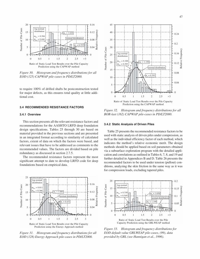
to require 100% of drilled shafts be postconstruction testedfor major defects, as this ensures total quality at little addi-tional cost.
3.4 RECOMMENDED RESISTANCE FACTORS
3.4.1 Overview
This section presents all the relevant resistance factors andrecommendations for the AASHTO LRFD deep foundationdesign specifications. Tables 25 through 30 are based onmaterial provided in the previous sections and are presentedin an integrated format according to similarity of calculatedfactors, extent of data on which the factors were based, andrelevant issues that have to be addressed as comments to therecommended values. The factors are divided based on pileredundancy as discussed in section 2.7.5.
The recommended resistance factors represent the mostsignificant attempt to date to develop LRFD code for deepfoundations based on empirical data.
47
3.4.2 Static Analysis of Driven Piles
Table 25 presents the recommended resistance factors to beused with static analysis of driven piles under compression, aswell as the individual efficiency factor of each method, whichindicates the method’s relative economic merit. The designmethods should be applied based on soil parameters obtainedvia a subsurface exploration program with the detailed appli-cation and correlations as outlined in Tables 6, 7, 8, and 19 andfurther detailed in Appendices B and D. Table 26 presents therecommended factors to be used under tension (pullout) con-ditions, analyzing the skin friction in the same way as it wasfor compression loads, excluding tapered piles.
0 0.5 1 1.5 2 2.5 3
Ratio of Static Load Test Results over the Pile CapacityPrediction using the CAPWAP method
0
5
10
15
20
Num
ber
of P
ile-
Cas
es
0
0.04
0.08
0.12
0.16
Rel
ativ
e Fr
eque
ncylog-normal
distribution
mlnx = 0.384
σlnx = 0.444 normal distribution
mx = 1.626
σx = 0.797
>
Figure 30. Histogram and frequency distributions for allEOD (125) CAPWAP pile-cases in PD/LT2000.
0 0.5 1 1.5 2 2.5 3
Ratio of Static Load Test Results over the Pile CapacityPrediction using the Energy Approach method
0
5
10
15
20
25
Num
ber
of P
ile-
Cas
es
0
0.04
0.08
0.12
0.16
Rel
ativ
e Fr
eque
ncy
log-normaldistribution
mlnx = 0.011
σlnx = 0.366
normal distribution
mx = 1.084
σx = 0.431
Figure 31. Histogram and frequency distributions for allEOD (128) Energy Approach pile-cases in PD/LT2000.
0 0.5 1 1.5 2 2.5 3
Ratio of Static Load Test Results over the Pile CapacityPrediction using the CAPWAP method
0
5
10
15
20
25
30
35
40
45
Num
ber
of P
ile-
Cas
es
0
0.04
0.08
0.12
0.16
0.2
0.24
Rel
ativ
e Fr
eque
ncy
log-normaldistribution
mlnx = 0.100
σlnx = 0.295
normal distribution
mx = 1.158
σx = 0.393
>
Figure 32. Histogram and frequency distributions for allBOR-last (162) CAPWAP pile-cases in PD/LT2000.
0 0.5 1 1.5 2 2.5 3
Ratio of Static Load Test Results over the PileCapacity Prediction using the GRLWEAP method
0
5
10
15
20
Num
ber
of P
ile-
Cas
es
0
0.05
0.1
0.15
0.2R
elat
ive
Freq
uenc
ylog-normaldistribution
mlnx = 0.330
σlnx = 0.549normal distribution
mx = 1.656
σx = 1.199
>
Figure 33. Histogram and frequency distributions forEOD default value GRLWEAP pile-cases, (99), dataprovided by GRL (see Hannigan et al., 1996).

The assigned resistance factors are based on the LRFDprinciple of a consistent prescribed reliability for either aredundant or a nonredundant pile cap configuration. The rec-ommended values should not be affected by the quality con-trol procedure to be implemented in the construction stageother than through the relationship with the anticipated ulti-mate capacity as explained in item 3 of section 3.4.7.
3.4.3 Dynamic Analysis of Driven Piles
Table 27 presents the recommended resistance factors tobe used for dynamic monitoring of driven piles and the rele-vant method’s efficiency factors. The dynamic methods arecategorized according to the controlling parameter and thetime of driving. Table 28 presents the recommended numberof tests required during production, with values rounded tothe next highest integer. Dynamic tests at EOD are carriedout for capacity evaluation, monitoring the performance ofthe driving system, and establishing driving criteria. As such,EOD tests are of great importance beyond the capacity eval-uation alone.
The following comments relate to the way site variabilityis being established:
1. Site variability relates to the variability within similarsubsurface conditions of the same site, not between sites.For example, when piers are based on substantially dif-ferent subsurface conditions (i.e., in the stratum mostlyinfluencing the pile capacity). The criteria should beapplied independently to each pier location as a sepa-rate site.
2. Site variability can be determined by judgment or usingthe following approximate criteria related to boringsrepresentative of the entire site subsurface conditions:
48
a. Relate to each significant bearing layer, averageparameters used for strength analysis (e.g., N SPT)at each boring location.
b. Check the COV between the average values foreach identifiable significant layer obtained at eachboring location.
c. Categorize site variability in the following way:i) COV < 25%—Low
ii) 25% ≤ COV < 40%—Mediumiii) 40% ≤ COV—High
The following recommendations apply to dynamic tests:1. Restrike should be scheduled according to the guide-
lines provided in section 3.4.62. The recommended values in Table 28 relate to similar
pile types driven at the same site.3. For EOD conditions:
• If dynamic measurements are available, evaluate pilecapacity using the Energy Approach; if dynamic mea-surements are not available, evaluate pile capacityusing the Gates or the FHWA modified Gates.
• Signal matching is recommended for EOD condi-tions for end bearing piles only.
0 0.5 1 1.5 2 2.5 3
Ratio of Static Load Test Results over the Pile CapacityPrediction using the Energy Approach method
0
5
10
15
20
25
30
Num
ber
of P
ile-
Cas
es
0
0.04
0.08
0.12
0.16
Rel
ativ
e Fr
eque
ncy
log-normaldistribution
mlnx = -0.304
σlnx = 0.350
normal distribution
mx = 0.785
σx = 0.290
Figure 34. Histogram and frequency distributions for allBOR-last (153) energy approach pile-cases in PD/LT2000.
Figure 35. Histogram and frequency distributions for all(384) FHWA modified Gates equation pile-cases inPD/LT2000.
0 0.5 1 1.5 2 2.5 3
Ratio of Static Load Test Results over the Pile Capacity PredictionAccording to the FHWA modified Gates equation
0
5
10
15
20
25
30
35
40
45
50
55
60
Num
ber
of P
ile-
Cas
es
0
0.01
0.02
0.03
0.04
0.05
0.06
0.07
0.08
0.09
0.1
0.11
0.12
0.13
0.14
0.15
Rel
ativ
e Fr
eque
ncy
log-normaldistribution
mlnx = -0.162
σlnx = 0.435
normal distribution
mx = 0.940
σx = 0.472
>
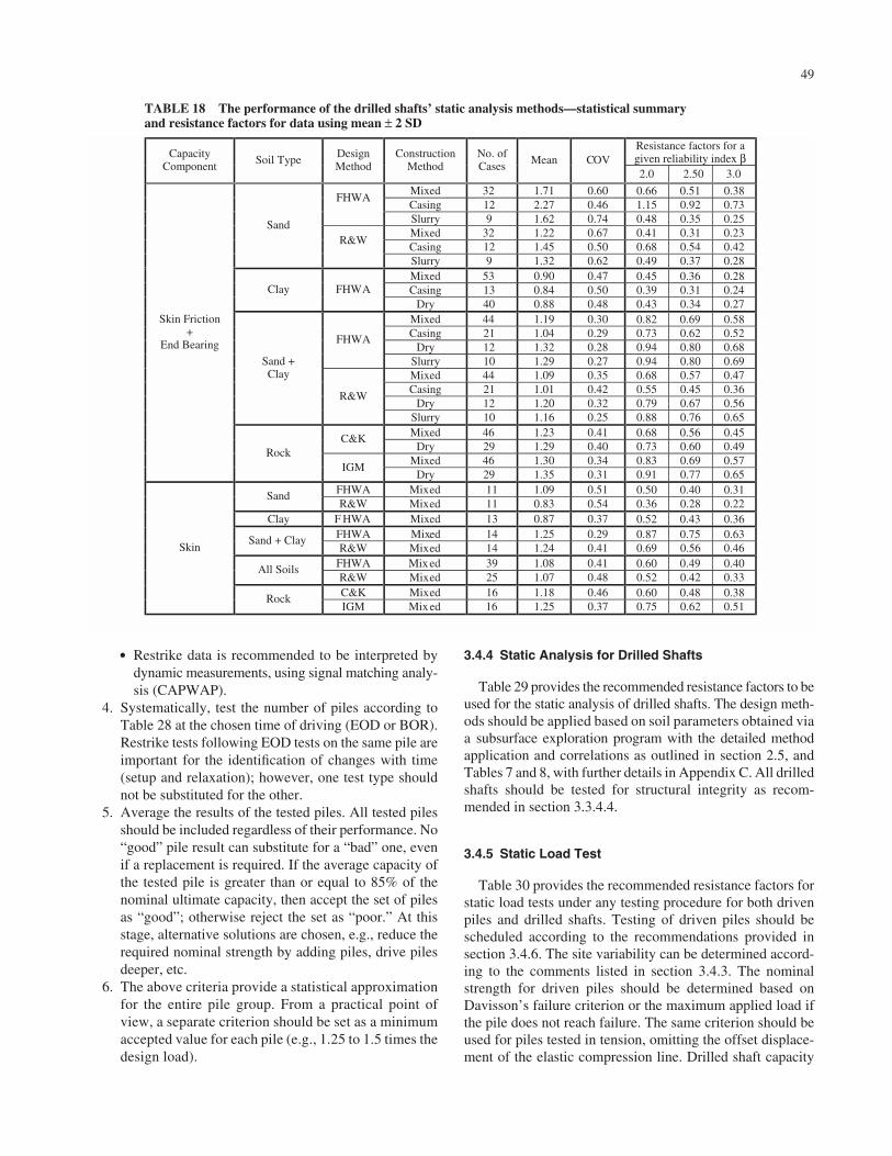
• Restrike data is recommended to be interpreted bydynamic measurements, using signal matching analy-sis (CAPWAP).
4. Systematically, test the number of piles according toTable 28 at the chosen time of driving (EOD or BOR).Restrike tests following EOD tests on the same pile areimportant for the identification of changes with time(setup and relaxation); however, one test type shouldnot be substituted for the other.
5. Average the results of the tested piles. All tested pilesshould be included regardless of their performance. No“good” pile result can substitute for a “bad” one, evenif a replacement is required. If the average capacity ofthe tested pile is greater than or equal to 85% of thenominal ultimate capacity, then accept the set of pilesas “good”; otherwise reject the set as “poor.” At thisstage, alternative solutions are chosen, e.g., reduce therequired nominal strength by adding piles, drive pilesdeeper, etc.
6. The above criteria provide a statistical approximationfor the entire pile group. From a practical point ofview, a separate criterion should be set as a minimumaccepted value for each pile (e.g., 1.25 to 1.5 times thedesign load).
49
3.4.4 Static Analysis for Drilled Shafts
Table 29 provides the recommended resistance factors to beused for the static analysis of drilled shafts. The design meth-ods should be applied based on soil parameters obtained viaa subsurface exploration program with the detailed methodapplication and correlations as outlined in section 2.5, andTables 7 and 8, with further details in Appendix C. All drilledshafts should be tested for structural integrity as recom-mended in section 3.3.4.4.
3.4.5 Static Load Test
Table 30 provides the recommended resistance factors forstatic load tests under any testing procedure for both drivenpiles and drilled shafts. Testing of driven piles should bescheduled according to the recommendations provided insection 3.4.6. The site variability can be determined accord-ing to the comments listed in section 3.4.3. The nominalstrength for driven piles should be determined based onDavisson’s failure criterion or the maximum applied load ifthe pile does not reach failure. The same criterion should beused for piles tested in tension, omitting the offset displace-ment of the elastic compression line. Drilled shaft capacity
Resistance factors for a given reliability index β Capacity
Component Soil Type Design Method
Construction Method
No. of Cases Mean COV
2.0 2.50 3.0
Mixed 32 1.71 0.60 0.66 0.51 0.38 Casing 12 2.27 0.46 1.15 0.92 0.73
FHWA
Slurry 9 1.62 0.74 0.48 0.35 0.25Mixed 32 1.22 0.67 0.41 0.31 0.23Casing 12 1.45 0.50 0.68 0.54 0.42
Sand R&W
Slurry 9 1.32 0.62 0.49 0.37 0.28Mixed 53 0.90 0.47 0.45 0.36 0.28 Casing 13 0.84 0.50 0.39 0.31 0.24Clay FHWA
Dry 40 0.88 0.48 0.43 0.34 0.27Mixed 44 1.19 0.30 0.82 0.69 0.58 Casing 21 1.04 0.29 0.73 0.62 0.52
Dry 12 1.32 0.28 0.94 0.80 0.68FHWA
Slurry 10 1.29 0.27 0.94 0.80 0.69Mixed 44 1.09 0.35 0.68 0.57 0.47Casing 21 1.01 0.42 0.55 0.45 0.36
Dry 12 1.20 0.32 0.79 0.67 0.56
Sand + Clay
R&W
Slurry 10 1.16 0.25 0.88 0.76 0.65Mixed 46 1.23 0.41 0.68 0.56 0.45 C&K
Dry 29 1.29 0.40 0.73 0.60 0.49Mixed 46 1.30 0.34 0.83 0.69 0.57
Skin Friction +
End Bearing
Rock IGM
Dry 29 1.35 0.31 0.91 0.77 0.65FHWA Mixed 11 1.09 0.51 0.50 0.40 0.31 Sand R&W Mixed 11 0.83 0.54 0.36 0.28 0.22
Clay F HWA Mixed 13 0.87 0.37 0.52 0.43 0.36 FHWA Mixed 14 1.25 0.29 0.87 0.75 0.63 Sand + Clay R&W Mixed 14 1.24 0.41 0.69 0.56 0.46
FHWA Mixed 39 1.08 0.41 0.60 0.49 0.40 All Soils R&W Mixed 25 1.07 0.48 0.52 0.42 0.33C&K Mixed 16 1.18 0.46 0.60 0.48 0.38
Skin
Rock IGM Mixed 16 1.25 0.37 0.75 0.62 0.51
TABLE 18 The performance of the drilled shafts’ static analysis methods—statistical summary and resistance factors for data using mean ± 2 SD
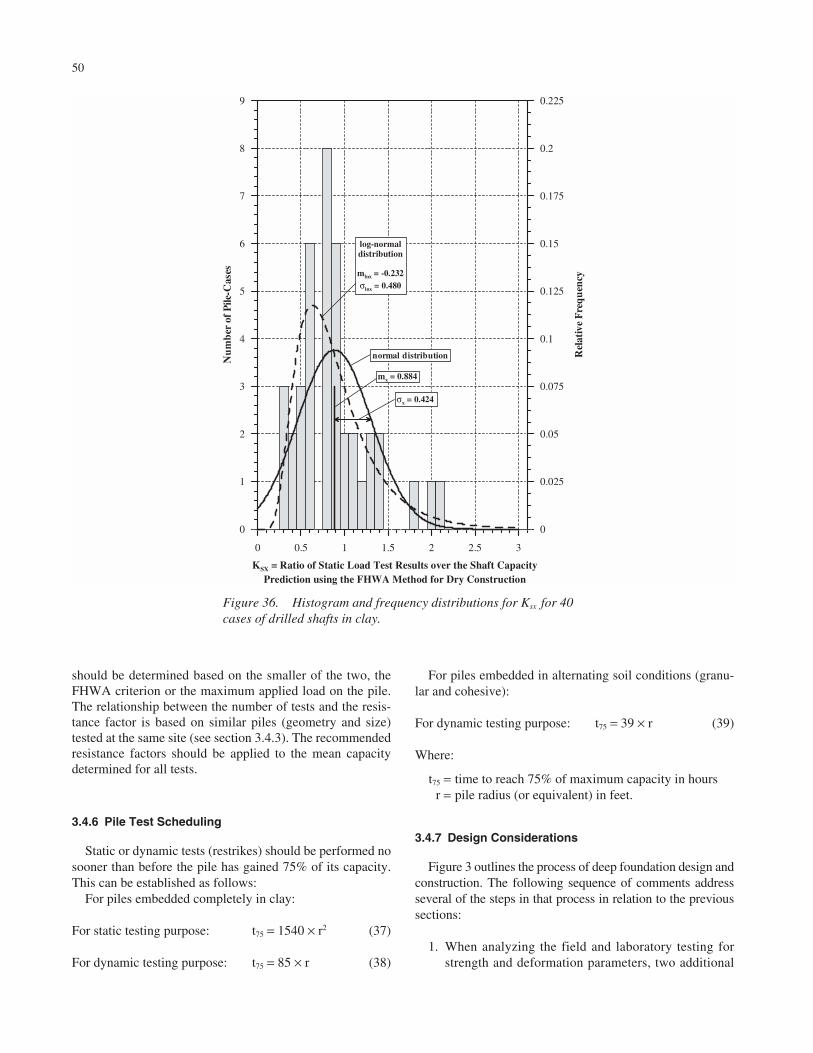
should be determined based on the smaller of the two, theFHWA criterion or the maximum applied load on the pile.The relationship between the number of tests and the resis-tance factor is based on similar piles (geometry and size)tested at the same site (see section 3.4.3). The recommendedresistance factors should be applied to the mean capacitydetermined for all tests.
3.4.6 Pile Test Scheduling
Static or dynamic tests (restrikes) should be performed nosooner than before the pile has gained 75% of its capacity.This can be established as follows:
For piles embedded completely in clay:
For static testing purpose: t75 = 1540 × r2 (37)
For dynamic testing purpose: t75 = 85 × r (38)
50
For piles embedded in alternating soil conditions (granu-lar and cohesive):
For dynamic testing purpose: t75 = 39 × r (39)
Where:
t75 = time to reach 75% of maximum capacity in hoursr = pile radius (or equivalent) in feet.
3.4.7 Design Considerations
Figure 3 outlines the process of deep foundation design andconstruction. The following sequence of comments addressseveral of the steps in that process in relation to the previoussections:
1. When analyzing the field and laboratory testing forstrength and deformation parameters, two additional
0 0.5 1 1.5 2 2.5 3
KSX = Ratio of Static Load Test Results over the Shaft CapacityPrediction using the FHWA Method for Dry Construction
0
1
2
3
4
5
6
7
8
9
Nu
mb
er o
f P
ile-C
ases
0
0.025
0.05
0.075
0.1
0.125
0.15
0.175
0.2
0.225
Rel
ativ
e F
req
uen
cy
log-normaldistribution
mlnx = -0.232σlnx = 0.480
mx = 0.884
σx = 0.424
normal distribution
Figure 36. Histogram and frequency distributions for Ksx for 40cases of drilled shafts in clay.
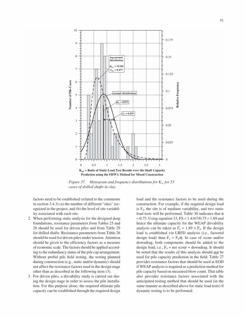
factors need to be established (related to the commentsin section 3.4.3) (a) the number of different “sites” rec-ognized in the project, and (b) the level of site variabil-ity associated with each site.
2. When performing static analysis for the designed deepfoundations, resistance parameters from Tables 25 and26 should be used for driven piles and from Table 29for drilled shafts. Resistance parameters from Table 26should be used for driven piles under tension. Attentionshould be given to the efficiency factors as a measureof economic scale. The factors should be applied accord-ing to the redundancy status of the pile cap arrangement.Without prebid pile field testing, the testing plannedduring construction (e.g., static and/or dynamic) shouldnot affect the resistance factors used in the design stageother than as described in the following item (3).
3. For driven piles, a drivability study is carried out dur-ing the design stage in order to assess the pile installa-tion. For this purpose alone, the required ultimate pilecapacity can be established through the required design
51
load and the resistance factors to be used during theconstruction. For example, if the required design loadis Fd, the site is of medium variability, and two staticload tests will be performed, Table 30 indicates that φ= 0.75. Using equation 33, FS = 1.4167/0.75 = 1.89 andhence the ultimate capacity for the WEAP drivabilityanalysis can be taken as Fu = 1.89 × Fd. If the designload is established via LRFD analysis (i.e., factoreddesign load) than Fu = Fd/φ. In case of scour and/ordowndrag, both components should be added to thedesign load, i.e., Fd + net scour + downdrag. It shouldbe noted that the results of this analysis should not beused for pile capacity prediction in the field. Table 27provides resistance factors that should be used at EODif WEAP analysis is required as a prediction method forpile capacity based on measured blow count. That tablealso provides resistance factors associated with theanticipated testing method that should be used (in thesame manner as described above for static load tests) ifdynamic testing is to be performed.
0 0.5 1 1.5 2 2.5 3
KSX = Ratio of Static Load Test Results over the Shaft CapacityPrediction using the FHWA Method for Mixed Construction
0
1
2
3
4
5
6
7
8
9
10
Nu
mb
er o
f Pile
-Cas
es
0
0.025
0.05
0.075
0.1
0.125
0.15
0.175
Rel
ativ
e F
req
uen
cy
log-normaldistribution
mlnx = -0.246σlnx = 0.477
mx = 0.872
σx = 0.419
normal distribution
Figure 37. Histogram and frequency distributions for Ksx for 53cases of drilled shafts in clay.

4. The determination of the required number of indicatorpiles can be combined along with the required numberof dynamic pile tests presented in Table 28. For sites atwhich fewer than 100 piles are driven, the number ofindicator piles can be used as the number of tested piles(approximately 8). Specifically, at least one pile shouldbe tested under each substructure, using the test resultsas outlined in section 3.3.3. When more than 100 pilesare driven, particularly at sites of high variability, sep-aration can be made between indicator piles and pro-duction piles, with the former used for assigning driv-ing criteria and the latter used for production qualitycontrol, as outlined in section 3.3.3. Restrike testing ofpiles should be scheduled according to equations 37through 39, as outlined in section 3.4.6.
5. Resistance factors for static load tests of driven piles anddrilled shafts should be assigned according to Table 30.The driven pile tests should be scheduled according toequations 37 through 39, as outlined in section 3.4.6.
6. All drilled shafts should be tested using small or highstrain integrity testing.
52
3.5 EVALUATION OF THE RESISTANCE FACTORS
3.5.1 Overview
Evaluation of the recommended resistance factors to beincorporated into a code is a complex and extensive process.The aim of the process is to compare an existing code ofpractice to the recommended new factors. Very often thisevaluation cannot be done directly, as either the principlesbehind the factors differ (e.g., WSD vs. LRFD), or the appliedmethodology is not compatible (e.g., the design and con-struction combined factors of the existing code). As a result,the evaluation can be carried out in two ways:
1. Analyzing design case histories in light of both the newfactors and the existing codes. In this way what hasbeen done can be compared with what would have beendone; and, if a sufficient number of case histories areanalyzed, statistically valid conclusions can be derivedregarding the effectiveness and overall performance ofthe recommendations.
0 0.5 1 1.5 2 2.5 3 3.5 4 4.5
KSX = Ratio of Static Load Test Results over the Shaft CapacityPrediction using the FHWA Method for Mixed Construction
0
0.5
1
1.5
2
2.5
3
3.5
4
Nu
mb
er o
f P
ile-C
ases
0
0.025
0.05
0.075
0.1
0.125
Rel
ativ
e F
req
uen
cy
log-normaldistribution
mlnx = 0.326σlnx = 0.738
mx = 1.714
σx = 1.027
normal distribution
Figure 38. Histogram and frequency distributions for Ksx for 32cases of drilled shafts in sand.
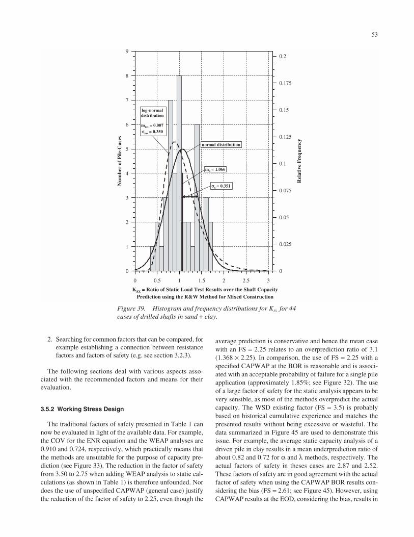
2. Searching for common factors that can be compared, forexample establishing a connection between resistancefactors and factors of safety (e.g. see section 3.2.3).
The following sections deal with various aspects asso-ciated with the recommended factors and means for theirevaluation.
3.5.2 Working Stress Design
The traditional factors of safety presented in Table 1 cannow be evaluated in light of the available data. For example,the COV for the ENR equation and the WEAP analyses are0.910 and 0.724, respectively, which practically means thatthe methods are unsuitable for the purpose of capacity pre-diction (see Figure 33). The reduction in the factor of safetyfrom 3.50 to 2.75 when adding WEAP analysis to static cal-culations (as shown in Table 1) is therefore unfounded. Nordoes the use of unspecified CAPWAP (general case) justifythe reduction of the factor of safety to 2.25, even though the
53
average prediction is conservative and hence the mean casewith an FS = 2.25 relates to an overprediction ratio of 3.1(1.368 × 2.25). In comparison, the use of FS = 2.25 with aspecified CAPWAP at the BOR is reasonable and is associ-ated with an acceptable probability of failure for a single pileapplication (approximately 1.85%; see Figure 32). The useof a large factor of safety for the static analysis appears to bevery sensible, as most of the methods overpredict the actualcapacity. The WSD existing factor (FS = 3.5) is probablybased on historical cumulative experience and matches thepresented results without being excessive or wasteful. Thedata summarized in Figure 45 are used to demonstrate thisissue. For example, the average static capacity analysis of adriven pile in clay results in a mean underprediction ratio ofabout 0.82 and 0.72 for α and λ methods, respectively. Theactual factors of safety in theses cases are 2.87 and 2.52.These factors of safety are in good agreement with the actualfactor of safety when using the CAPWAP BOR results con-sidering the bias (FS = 2.61; see Figure 45). However, usingCAPWAP results at the EOD, considering the bias, results in
0 0.5 1 1.5 2 2.5 3
KSX = Ratio of Static Load Test Results over the Shaft CapacityPrediction using the R&W Method for Mixed Construction
0
1
2
3
4
5
6
7
8
9
Nu
mb
er o
f P
ile-C
ases
0
0.025
0.05
0.075
0.1
0.125
0.15
0.175
0.2
Rel
ativ
e F
req
uen
cy
log-normaldistribution
mlnx = 0.007σlnx = 0.350
mx = 1.066
σx = 0.351
normal distribution
Figure 39. Histogram and frequency distributions for Ksx for 44cases of drilled shafts in sand + clay.

54
0 0.5 1 1.5 2 2.5 3
KSX = Ratio of Static Load Test Results over the Shaft CapacityPrediction using the C&K Method for Mixed Construction
0
0.5
1
1.5
2
2.5
3
3.5
4
4.5
5
5.5
6
Nu
mb
er o
f P
ile-C
ases
0
0.02
0.04
0.06
0.08
0.1
0.12
Rel
ativ
e F
req
uen
cy
log-normaldistribution
mlnx = 0.101σlnx = 0.494
mx = 1.229
σx = 0.509
normal distribution
Figure 40. Histogram and frequency distributions for Ksx for 46 cases of drilled shafts in rock.
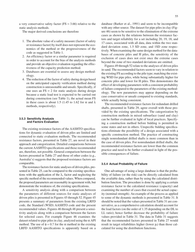
55
a very conservative safety factor (FS = 3.66) relative to thestatic analysis methods.
The major derived conclusions are therefore
1. The absolute value of a safety measure (factor of safetyor resistance factor) by itself does not represent the eco-nomics of the method or the progressiveness of thecode as suggested in Table 1.
2. An efficiency factor or a similar parameter is requiredin order to account for the bias of the analysis methodsand provide an objective evaluation regarding the effec-tiveness of the capacity prediction method.
3. Databases are essential to assess any design method-ology.
4. The reduction of the factor of safety during design basedon the anticipated capacity verification method duringconstruction is unreasonable and unsafe. Specifically, ifone uses an FS = 2 for static analysis during designbecause a static load test is expected to be carried outduring construction (see Table 1), the actual mean FSin these cases is about 1.5 (1.45 to 1.62 for α and λmethods, respectively).
3.5.3 Sensitivity Analysis and Factors Evaluation
The existing resistance factors of the AASHTO specifica-tions for dynamic evaluation of driven piles are limited andconnected to static evaluation methods. The recommendedresistance factors, presented in Table 27, are novel in theirapproach and categorization. Detailed comparisons betweenthe current AASHTO specifications and those recommendedare, therefore, not possible. General comparison between thefactors presented in Table 27 and those of other codes (e.g.,Australia’s) suggests that the proposed resistance factors arecomparable.
The resistance factors for static analyses of driven piles, pre-sented in Table 25, can be compared to the existing specifica-tions with the application of the λv factor and neglecting thespecific method of the recommended values. When compared,the proposed parameters are reasonably in agreement with, butdemonstrate the weakness of, the existing specifications.
A sensitivity analysis along with a comparison betweenthe parameters of different sources for static analyses ofdriven piles is presented in Figures 45 through 52. Figure 45presents a summary of parameters from the existing LRFDcode, the Standard (WSD) AASHTO code and the presentrecommended values. Figures 46 through 48 present a sensi-tivity analysis along with a comparison between the factorsfor selected cases. For example Figure 46 examines thedataset related to pipe piles in clay, analyzed using the α APImethod. The use of φ = 0.7 for the α method in the existingLRFD AASHTO specifications is apparently based on a
database (Barker et al., 1991) and seem to be incompatiblewith any other source. The dataset for pipe piles in clay (Fig-ure 46) seem to be sensitive to the elimination of the extremecases as shown by the relations between the resistance fac-tors and target reliability for a set including 20, 19, 18, and17 cases, associated with all data, data within the two stan-dard deviation zone, 1.5 SD zone, and 1SD zone respec-tively. When examining the same design method for the data-bases of concrete piles and H piles, the sensitivity of theexclusion of cases does not exist once the extreme casesbeyond the zone of two standard deviations are omitted.
Figures 49 through 52 relate to the analyses of driven pilesin sand. The recommended factors seem to vary in relation tothe existing FS according to the pile type; matching the exist-ing WSD for pipe piles, while being substantially higher forconcrete piles and lower for H piles. This demonstrates theeffect of developing parameters with a consistent probabilityof failure compared to the parameters of the existing method-ology. The new parameters may appear depending on thecase conservative or unsafe compared to existing standards,while actually being consistent.
The recommended resistance factors for redundant drilledshafts, presented in Table 29, agree overall with those pro-vided by the existing specifications. The categorization byconstruction methods in mixed subsurface (sand and clay)can be further evaluated in light of local practices. Specify-ing a construction method before bidding is permitted insome states and not in others. Unspecific bidding specifica-tions eliminate the possibility of a design associated with aspecific construction method. The practice of constructingsingle nonredundant drilled shafts is more common than inthe case of driven piles. For nonredundant drilled shafts, therecommended resistance factors are lower than the commonpractice and need to be further evaluated in light of the pos-sible consequences of failure.
3.5.4 Actual Probability of Failure
One advantage of using a large database is that the proba-bility of failure (or the risk) can be directly calculated fromthe available data, rather than by using the calculated distri-bution function. The procedure is done by applying a certainresistance factor to the calculated resistance (capacity) andexamining the number of cases that exceed the actual capac-ity (nominal strength). An example of the process as appliedto some of the dynamic methods is presented in Table 31. Itshould be noted that the values presented in Table 31 are con-servative, as a comprehensive calculation should account forthe load factors (on the order of 1.35 depending on the DL toLL ratio); hence further decrease the probability of failurevalues provided in Table 31. The data in Table 31 suggeststhat the recommended factors presented in Table 27 wouldresult in target reliabilities higher (lower pf) than those cal-culated for using the distribution functions.
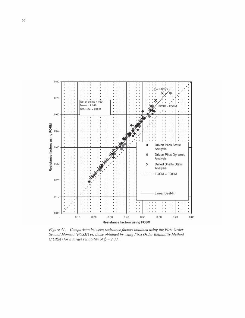
56
.
y = 1.1267x
0.00
0.10
0.20
0.30
0.40
0.50
0.60
0.70
0.80
- 0.10 0.20 0.30 0.40 0.50 0.60 0.70 0.80
Resistance factors using FOSM
Res
ista
nce
fac
tors
usi
ng
FO
RM
Driven Piles StaticAnalysis
Driven Piles DynamicAnalysis
Drilled Shafts StaticAnalysis
FOSM = FORM
Linear Best-fit
No. of points = 160Mean = 1.148Std. Dev. = 0.039
FOSM = FORM
Figure 41. Comparison between resistance factors obtained using the First OrderSecond Moment (FOSM) vs. those obtained by using First Order Reliability Method(FORM) for a target reliability of β = 2.33.
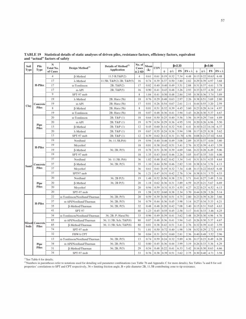
57
β=2.33β=2.33β=2.33β=2.33 β=3β=3.00β=3.00β=3.00 Soil Type
Pile Type
N Total No. of Cases
Design Method(1) Details of Method(2)
Application
No. of Cases ±±±± 2 SD
Mean (λλλλ)
COV φ φ/λ FS FS x λ φ φ/λ FS FS x λ
4 β-Method 11.5 B;T&P(2) 4 0.61 0.61 0.19 0.32 7.34 4.48 0.13 0.22 10.63 6.48
17 λ-Method 11.5B; T&P(2) 2B; T&P(5) 16 0.74 0.39 0.37 0.50 3.80 2.82 0.29 0.39 4.97 3.68
17 α-Tomlinson 2B; T&P(2) 17 0.82 0.40 0.40 0.49 3.51 2.88 0.31 0.37 4.61 3.78
17 α-API 2B; T&P(5) 16 0.90 0.41 0.43 0.48 3.26 2.93 0.33 0.37 4.30 3.87
H-Piles
9 SPT-97 mob 8 1.04 0.41 0.50 0.48 2.84 2.95 0.38 0.36 3.74 3.89
19 λ-Method 2B; Hara (5h) 18 0.76 0.29 0.48 0.63 2.97 2.26 0.38 0.51 3.69 2.80
19 α-API 2B; Hara (5h) 17 0.81 0.26 0.54 0.67 2.61 2.11 0.44 0.55 3.20 2.59
8 β-Method 2B; Hara (5h) 8 0.81 0.51 0.32 0.39 4.45 3.60 0.23 0.28 6.14 4.97
Concrete Piles
19 α-Tomlinson 2B; Hara (5h) 18 0.87 0.48 0.36 0.41 3.94 3.43 0.26 0.30 5.37 4.67
20 α-Tomlinson 2B; T&P (1) 18 0.64 0.50 0.25 0.40 5.56 3.56 0.19 0.29 7.64 4.89
20 α-API 2B; T&P (1) 19 0.79 0.54 0.29 0.36 4.95 3.91 0.20 0.26 6.96 5.50
13 β-Method 2B; T&P (1) 12 0.45 0.60 0.14 0.32 9.81 4.41 0.10 0.22 14.16 6.37
20 λ-Method 2B; T&P (1) 19 0.67 0.55 0.24 0.36 5.94 3.98 0.17 0.25 8.38 5.62
Clay
Pipe Piles
13 SPT-97 mob 2B; T&P (1) 12 0.39 0.62 0.12 0.31 11.70 4.56 0.08 0.21 17.02 6.64
19 Nordlund 36; 11.5B,P(6) 19 0.94 0.40 0.46 0.49 3.08 2.89 0.35 0.37 4.04 3.80
19 Meyerhof 18 0.81 0.38 0.42 0.51 3.41 2.76 0.32 0.39 4.43 3.59
19 β-Method 36; 2B; P(5) 19 0.78 0.51 0.30 0.39 4.69 3.66 0.22 0.28 6.49 5.06 H-Piles
19 SPT-97 mob 18 1.35 0.43 0.63 0.46 2.26 3.05 0.47 0.35 3.01 4.06
37 Nordlund 36: 11.5B; P(6) 36 1.02 0.48 0.42 0.42 3.34 3.41 0.31 0.31 4.55 4.64
37 β-Method 36; 2B; P(5) 35 1.10 0.44 0.50 0.46 2.82 3.10 0.38 0.34 3.76 4.13
37 Meyerhof 36 0.61 0.61 0.19 0.32 7.34 4.48 0.13 0.22 10.63 6.48
Concrete Piles
37 SPT97 mob 36 1.21 0.47 0.51 0.42 2.76 3.34 0.38 0.31 3.75 4.53
20 Nordlund 36; 2B P(5) 19 1.48 0.52 0.56 0.38 2.51 3.71 0.41 0.27 3.49 5.16
20 β-Method 36; 2B P(5) 20 1.18 0.62 0.36 0.31 3.89 4.59 0.25 0.21 5.67 6.69
20 Meyerhof 20 0.94 0.59 0.31 0.33 4.55 4.27 0.22 0.23 6.52 6.13
Sand
Pipe Piles
20 SPT-97 mob 19 1.58 0.52 0.60 0.38 2.34 3.70 0.44 0.28 3.26 5.14
22 α-Tomlinson/Nordlund/Thurman 36; 2B; P(5) 20 0.59 0.39 0.30 0.51 4.75 2.80 0.23 0.39 6.20 3.66
37 α-API/Nordlund/Thurman 36; 2B; P(5) 34 0.79 0.44 0.36 0.45 3.98 3.14 0.27 0.34 5.33 4.21
35 β-Method/Thurman 36; 2B; P(5) 32 0.48 0.48 0.20 0.42 7.08 3.40 0.15 0.31 9.65 4.63 H-Piles
41 SPT-97 40 1.23 0.45 0.55 0.45 2.58 3.17 0.41 0.33 3.46 4.25
34 α-Tomlinson/Nordlund/Thurman 36; 2B; P; Hara(5h) 33 0.96 0.49 0.39 0.41 3.62 3.48 0.29 0.30 4.96 4.76
85 α-API/Nordland/Thurman 36; 11.5B; Sch; T&P(8) 80 0.87 0.48 0.36 0.41 3.94 3.43 0.26 0.30 5.37 4.67
85 β-Method/Thurman 36; 11.5B; Sch; T&P(8) 80 0.81 0.38 0.42 0.51 3.41 2.76 0.32 0.39 4.43 3.59
74 SPT-97 mob 71 1.81 0.50 0.72 0.40 1.98 3.58 0.52 0.29 2.72 4.93
Concrete Piles
32 FHWA CPT 30 0.84 0.31 0.51 0.60 2.81 2.36 0.40 0.48 3.52 2.96
13 α-Tomlinson/Nordlund/Thurman 36; 2B; P(5) 13 0.74 0.59 0.24 0.32 5.89 4.36 0.17 0.23 8.49 6.28
34 α-API/Nordland/Thurman 36; 2B; P(5) 32 0.80 0.45 0.36 0.44 3.99 3.19 0.26 0.33 5.36 4.29
31 β-Method/Thurman 36; 2B; P(5) 29 0.54 0.48 0.22 0.41 6.33 3.42 0.16 0.30 8.63 4.66
Mixed Soils
Pipe Piles
34 SPT-97 mob 33 0.76 0.38 0.39 0.51 3.62 2.75 0.30 0.40 4.71 3.58
(1)See Table 6 for details; (2)Numbers in parentheses refer to notations used for detailing soil parameter combinations (see Table 7b and Appendix C for more details), See Tables 7a and 8 for soil properties’ correlations to SPT and CPT respectively, 36 = limiting friction angle, B = pile diameter 2B, 11.5B contributing zone to tip resistance.
TABLE 19 Statistical details of static analyses of driven piles, resistance factors, efficiency factors, equivalent and “actual” factors of safety
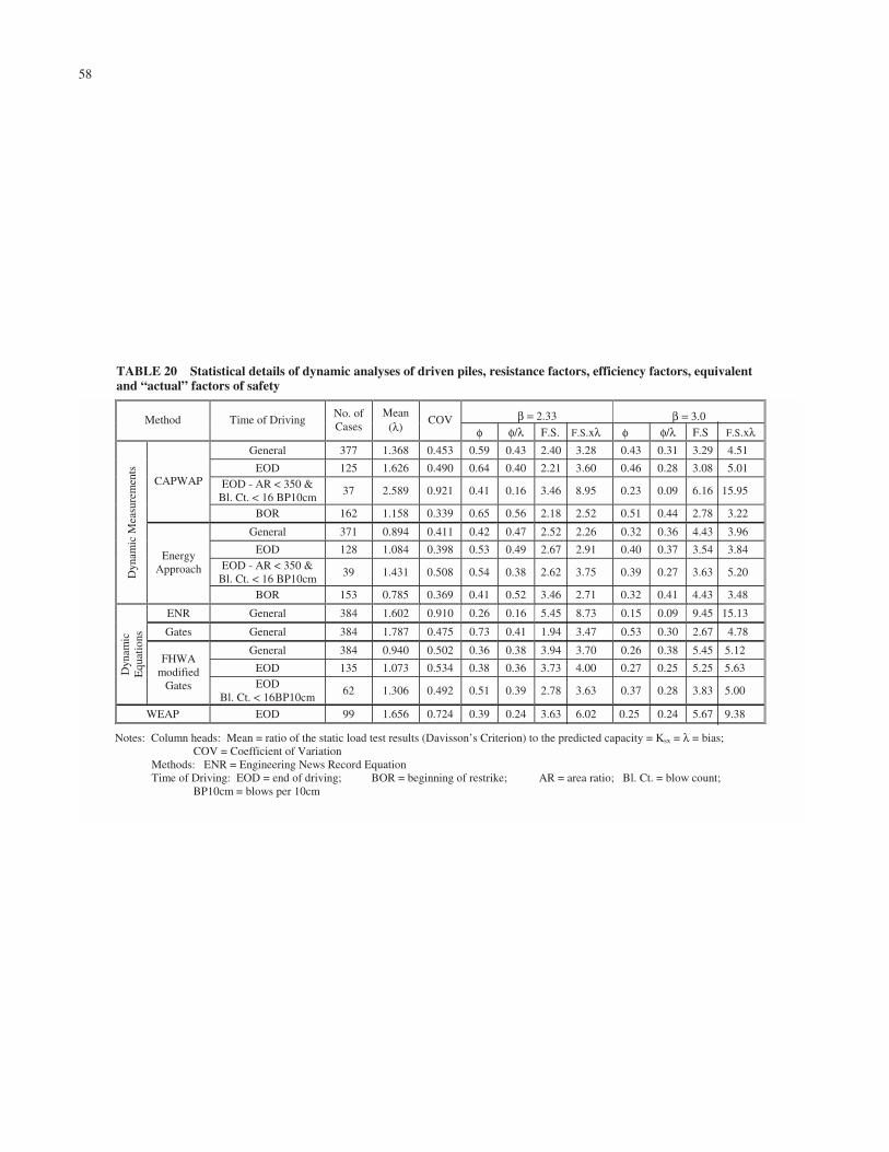
58
β = 2.33 β = 3.0 Method Time of Driving No. of Cases
Mean (λ)
COV φ φ/λ F.S. F.S.xλ φ φ/λ F.S F.S.xλ
General 377 1.368 0.453 0.59 0.43 2.40 3.28 0.43 0.31 3.29 4.51
EOD 125 1.626 0.490 0.64 0.40 2.21 3.60 0.46 0.28 3.08 5.01 EOD - AR < 350 &
Bl. Ct. < 16 BP10cm 37 2.589 0.921 0.41 0.16 3.46 8.95 0.23 0.09 6.16 15.95
CAPWAP
BOR 162 1.158 0.339 0.65 0.56 2.18 2.52 0.51 0.44 2.78 3.22
General 371 0.894 0.411 0.42 0.47 2.52 2.26 0.32 0.36 4.43 3.96
EOD 128 1.084 0.398 0.53 0.49 2.67 2.91 0.40 0.37 3.54 3.84 EOD - AR < 350 &
Bl. Ct. < 16 BP10cm 39 1.431 0.508 0.54 0.38 2.62 3.75 0.39 0.27 3.63 5.20 D
ynam
ic M
easu
rem
ents
Energy Approach
BOR 153 0.785 0.369 0.41 0.52 3.46 2.71 0.32 0.41 4.43 3.48
ENR General 384 1.602 0.910 0.26 0.16 5.45 8.73 0.15 0.09 9.45 15.13
Gates General 384 1.787 0.475 0.73 0.41 1.94 3.47 0.53 0.30 2.67 4.78
General 384 0.940 0.502 0.36 0.38 3.94 3.70 0.26 0.38 5.45 5.12
EOD 135 1.073 0.534 0.38 0.36 3.73 4.00 0.27 0.25 5.25 5.63 Dyn
amic
E
quat
ions
FHWA modified
Gates EOD Bl. Ct. < 16BP10cm
62 1.306 0.492 0.51 0.39 2.78 3.63 0.37 0.28 3.83 5.00
WEAP EOD 99 1.656 0.724 0.39 0.24 3.63 6.02 0.25 0.24 5.67 9.38
Notes: Column heads: Mean = ratio of the static load test results (Davisson’s Criterion) to the predicted capacity = Ksx = λ = bias; COV = Coefficient of Variation
Methods: ENR = Engineering News Record Equation Time of Driving: EOD = end of driving; BOR = beginning of restrike; AR = area ratio; Bl. Ct. = blow count;
BP10cm = blows per 10cm
TABLE 20 Statistical details of dynamic analyses of driven piles, resistance factors, efficiency factors, equivalentand “actual” factors of safety
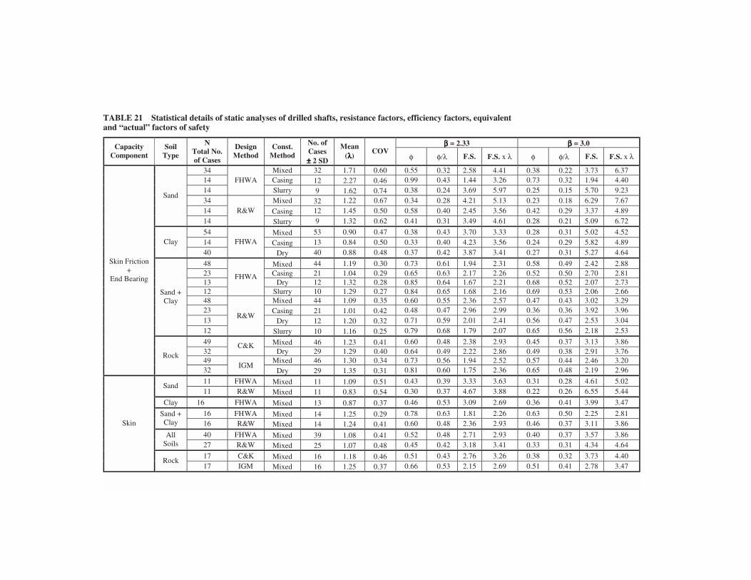
ββββ = 2.33 ββββ = 3.0 Capacity Component
Soil Type
N Total No. of Cases
Design Method
Const. Method
No. of Cases ±±±± 2 SD
Mean (λλλλ)
COV φ φ/λ F.S. F.S. x λ φ φ/λ F.S. F.S. x λ
34 Mixed 32 1.71 0.60 0.55 0.32 2.58 4.41 0.38 0.22 3.73 6.3714 Casing 12 2.27 0.46 0.99 0.43 1.44 3.26 0.73 0.32 1.94 4.4014
FHWA Slurry 9 1.62 0.74 0.38 0.24 3.69 5.97 0.25 0.15 5.70 9.23
34 Mixed 32 1.22 0.67 0.34 0.28 4.21 5.13 0.23 0.18 6.29 7.6714 Casing 12 1.45 0.50 0.58 0.40 2.45 3.56 0.42 0.29 3.37 4.89
Sand
14 R&W
Slurry 9 1.32 0.62 0.41 0.31 3.49 4.61 0.28 0.21 5.09 6.72
54 Mixed 53 0.90 0.47 0.38 0.43 3.70 3.33 0.28 0.31 5.02 4.5214 Casing 13 0.84 0.50 0.33 0.40 4.23 3.56 0.24 0.29 5.82 4.89Clay
40
FHWA
Dry 40 0.88 0.48 0.37 0.42 3.87 3.41 0.27 0.31 5.27 4.64
48 Mixed 44 1.19 0.30 0.73 0.61 1.94 2.31 0.58 0.49 2.42 2.8823 Casing 21 1.04 0.29 0.65 0.63 2.17 2.26 0.52 0.50 2.70 2.8113 Dry 12 1.32 0.28 0.85 0.64 1.67 2.21 0.68 0.52 2.07 2.7312
FHWA
Slurry 10 1.29 0.27 0.84 0.65 1.68 2.16 0.69 0.53 2.06 2.6648 Mixed 44 1.09 0.35 0.60 0.55 2.36 2.57 0.47 0.43 3.02 3.2923 Casing 21 1.01 0.42 0.48 0.47 2.96 2.99 0.36 0.36 3.92 3.9613 Dry 12 1.20 0.32 0.71 0.59 2.01 2.41 0.56 0.47 2.53 3.04
Sand + Clay
12
R&W
Slurry 10 1.16 0.25 0.79 0.68 1.79 2.07 0.65 0.56 2.18 2.53
49 Mixed 46 1.23 0.41 0.60 0.48 2.38 2.93 0.45 0.37 3.13 3.8632
C&K Dry 29 1.29 0.40 0.64 0.49 2.22 2.86 0.49 0.38 2.91 3.76
49 Mixed 46 1.30 0.34 0.73 0.56 1.94 2.52 0.57 0.44 2.46 3.20
Skin Friction +
End Bearing
Rock
32 IGM
Dry 29 1.35 0.31 0.81 0.60 1.75 2.36 0.65 0.48 2.19 2.96
11 FHWA Mixed 11 1.09 0.51 0.43 0.39 3.33 3.63 0.31 0.28 4.61 5.02Sand
11 R&W Mixed 11 0.83 0.54 0.30 0.37 4.67 3.88 0.22 0.26 6.55 5.44
Clay 16 FHWA Mixed 13 0.87 0.37 0.46 0.53 3.09 2.69 0.36 0.41 3.99 3.47
16 FHWA Mixed 14 1.25 0.29 0.78 0.63 1.81 2.26 0.63 0.50 2.25 2.81Sand + Clay 16 R&W Mixed 14 1.24 0.41 0.60 0.48 2.36 2.93 0.46 0.37 3.11 3.86
40 FHWA Mixed 39 1.08 0.41 0.52 0.48 2.71 2.93 0.40 0.37 3.57 3.86All Soils 27 R&W Mixed 25 1.07 0.48 0.45 0.42 3.18 3.41 0.33 0.31 4.34 4.64
17 C&K Mixed 16 1.18 0.46 0.51 0.43 2.76 3.26 0.38 0.32 3.73 4.40
Skin
Rock 17 IGM Mixed 16 1.25 0.37 0.66 0.53 2.15 2.69 0.51 0.41 2.78 3.47
TABLE 21 Statistical details of static analyses of drilled shafts, resistance factors, efficiency factors, equivalentand “actual” factors of safety

60
β = 2.33 β = 3.00 γL = 1.75, γD = 1.2, DL/LL = 2
Category Pile Type or Construction
Soil Type or State
Method of Analysis φ
resistance factor
φ/λ efficiency
FS factor of
safety
FS x λ actual
mean FS
PPC Clay α - API 0.54 0.44
0.67 0.55
2.61 3.20
2.11 2.59
PPC Sand β 0.50 0.38
0.46 0.34
2.82 3.76
3.10 4.13
Static Methods Driven Piles
Pipe Mixed α - API Nordlund/Thurman
0.36 0.26
0.44 0.33
3.99 5.36
3.19 4.29
All BOR CAPWAP 0.65 0.51
0.56 0.44
2.18 2.78
2.52 3.22
All Energy Approach 0.53 0.40
0.49 0.37
2.67 3.54
2.91 3.84
Dynamic Methods
Driven Piles All EOD FHWA mod Gates 0.38
0.27 0.36 0.25
3.73 5.25
4.00 5.63
Mixed All R&W skin 0.45 0.33
0.42 0.31
3.18 4.34
3.41 4.64
Mixed Rock C&K total 0.60 0.45
0.48 0.37
2.38 3.13
2.93 3.86
Static Methods Drilled Shafts
Mixed Sand & Clay FHWA skin 0.78 0.63
0.63 0.50
1.81 2.25
2.26 2.81
Notes: *Top line of column: β = 2.33; **Bottom line of column: β = 3.00; γL = 1.75; γD = 1.2; DL/LL = 2.
EOD
Resistance Factor φ/λ
Pile Type
Soil Type
Design Method
No.
λ COV Redundant β = 2.33
Non-redundant β = 3.00
Redundant β = 2.33
Non-redundant β = 3.00
α-API 9 1.11 0.71 0.28 0.18 0.25 0.16 α-Tomlinson 9 0.95 0.57 0.33 0.23 0.35 0.24Clay
λ-Method 9 0.72 0.52 0.27 0.20 0.38 0.36β-Method 7 0.52 0.54 0.19 0.14 0.37 0.27
SPT-97 mob 7 1.18 1.33 0.08 0.04 0.07 0.03
Pipe Sand and
Mixed αAPI/Nordlund 7 0.80 0.60 0.26 0.18 0.33 0.23α-API 3 0.76 0.57 0.26 0.18 0.34 0.24
Clay α-Tomlinson 3 0.64 0.54 0.23 0.17 0.36 0.27
β-Method 8 0.23 0.36 0.12 0.10 0.52 0.43H
Sand SPT-97 mob 0.43 0.32 0.25 0.20 0.58 0.478
Target Reliability β Site Variation N Mean
(λ) (Bias)
SD C.O.V.
2.00 2.33 3.00 1 1 0.18 0.18 0.86 0.80 0.672 1 0.13 0.13 0.96 0.89 0.783 1 0.10 0.10 1.00 0.94 0.834 1 0.09 0.09 1.03 0.97 0.86
Low
5 1 0.08 0.08 1.04 0.99 0.881 1 0.27 0.27 0.73 0.65 0.532 1 0.19 0.19 0.85 0.78 0.663 1 0.16 0.16 0.90 0.84 0.724 1 0.14 0.14 0.94 0.88 0.76
Medium
5 1 0.12 0.12 0.97 0.90 0.791 1 0.36 0.36 0.61 0.54 0.422 1 0.25 0.25 0.75 0.68 0.553 1 0.21 0.21 0.82 0.75 0.634 1 0.18 0.18 0.86 0.80 0.67
High
5 1 0.16 0.16 0.90 0.83 0.71
Note: N = Number of load tests
TABLE 22 Resistance factors and associated factors of safety along with efficiency measures for sample methods
TABLE 23 Detailed resistance factors for pullout of driven piles—based on static analyses
TABLE 24 Resistance factors as a function of number of load tests per site, site variability and target reliability
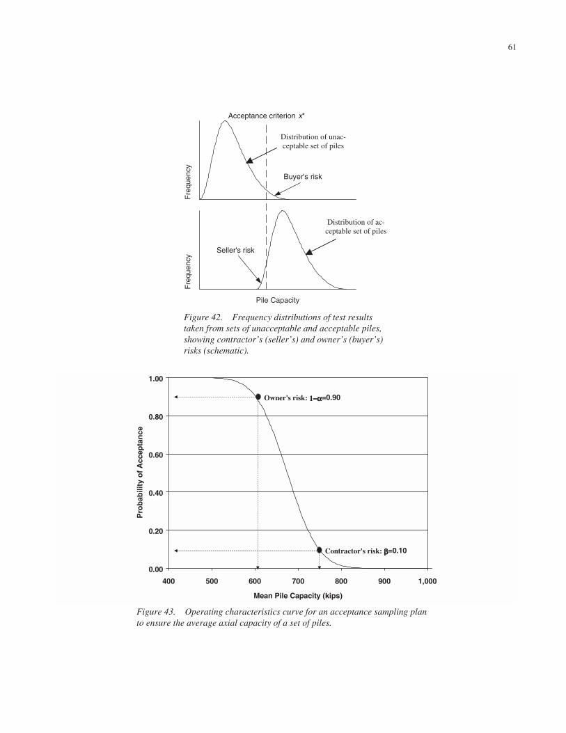
61
Fre
quen
cyF
requ
ency
Pile Capacity
Acceptance criterion x*
Seller's risk
Buyer's risk
Distribution of unac-ceptable set of piles
Distribution of ac-ceptable set of piles
Figure 42. Frequency distributions of test resultstaken from sets of unacceptable and acceptable piles,showing contractor’s (seller’s) and owner’s (buyer’s)risks (schematic).
0.00
0.20
0.40
0.60
0.80
1.00
400 500 600 700 800 900 1,000
Mean Pile Capacity (kips)
Pro
bab
ility
of
Acc
epta
nce
Contractor's risk: β β β β=0.10
Owner's risk: 1−α 1−α 1−α 1−α=0.90
Figure 43. Operating characteristics curve for an acceptance sampling planto ensure the average axial capacity of a set of piles.

62
2110
0.01 0.1
0.90
0.05
Figure 44. Binomial nomograph for determining sample size, n, and permitted number of defectives, c,for contractor’s risk α and owner’s risk β (Montgomery 1991). The procedure for using the nomograph todesign a sampling plan is to (1) draw a line connecting α on the right-hand rule with the corresponding p1
on the left-hand rule, (2) draw a similar line connecting (1-β) and p2, and (3) the point of intersection ofthe two lines gives the required sample size, n, and the maximum number of defectives permitted within thesample for acceptance.
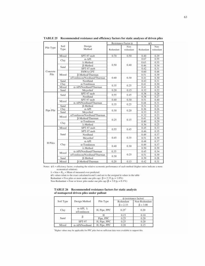
63
Resistance Factor φ φ/λ
Pile Type Soil Type
Design Method Redundant
Non-redundant
Redundant
Non-redundant
Mixed SPT-97 mob 0.70 0.50 0.40 0.29
α-API 0.67 0.55 Clay λ-Method 0.63 0.55β-Method 0.46 0.34Sand
SPT-97 mob 0.42 0.31 FHWA CPT
0.50 0.40
0.60 0.48β-Method/Thurman 0.51 0.39Mixed
αTomlinson/Nordlund/Thurman 0.41 0.30Sand Nordlund
0.40 0.300.42 0.31
Clay α-Tomlinson 0.41 0.30Mixed α-API/Nordlund/Thurman
0.35 0.250.41 0.30
Concrete Pile
Sand Meyerhof 0.20 0.15 0.32 0.22SPT-97 mob 0.38 0.28 Sand
Nordlund 0.55 0.45
0.38 0.27SPT-97 mob 0.40 0.30 0.51 0.40 Mixed α-API/Nordlund/Thurman 0.44 0.31
Sand β-Method 0.35 0.25
0.31 0.21Clay α-API 0.36 0.26Sand Meyerhof
0.30 0.200.33 0.23
αTomlinson/Nordlund/Thurman 0.32 0.23Mixed β-Method/Thurman 0.41 0.30α-Tomlinson 0.40 0.29
. Pipe Pile
Clay λ-Method
0.25 0.15
0.36 0.25Mixed SPT-97 mob 0.45 0.33
SPT-97 mob 0.55 0.45
0.46 0.35Nordlund 0.49 0.37Sand Meyerhof 0.51 0.39
α-API 0.45 0.35
0.48 0.37α-Tomlinson 0.49 0.37Clay
λ-Method 0.40 0.30
0.50 0.39α-API/Nordlund/Thurman 0.35 0.45 0.34Mixed
αTomlinson/Nordlund/Thurman 0.51 0.39Sand β-Method
0.30 0.25
0.39 0.28
H Piles
Mixed β-Method/Thurman 0.20 0.15 0.42 0.31
Notes: φ/λ = efficiency factor, evaluating the relative economic performance of each method (higher ratios indicate a more economical solution).
λ = bias = Ksx = Mean of measured over predicted. φ/λ values relate to the exact calculated φ and λ and not to the assigned φ values in the table Redundant = Five piles or more under one pile cap ( β = 2.33 pf = 1.0%) Non-Redundant = Four or fewer piles under one pile cap (β = 3.0 pf = 0.1%)
1Higher values may be applicable for PPC piles but no sufficient data were available to support this.
φ (resistance factor) Soil Type Design Method Pile Type Redundant
β = 2.33 Non-Redundant
β = 3.00
Clay α-API, λ
αTomlinson H, Pipe, PPC 0.251 0.20
H 0.15 0.10 β Pipe, PPC 0.25 0.20 Sand
SPT-97 H, Pipe, PPC 0.25 0.20 Mixed α-API/Nordlund H, Pipe, PPC 0.20 0.15
TABLE 25 Recommended resistance and efficiency factors for static analyses of driven piles
TABLE 26 Recommended resistance factors for static analysis of nontapered driven piles under pullout

64
φ (resistance factor) φ/ λ
Method Case Redundant
Non-Redundant
Redundant
Non-Redundant
EOD 0.65 0.45 0.40 0.28
EOD, AR<350, Bl. Ct.<16BP10cm 0.40 0.25 0.16 0.09
Signal Matching
(CAPWAP) BOR 0.65 0.50 0.56 0.44
EOD 0.55 0.40 0.49 0.37
Dynamic Measurements
Energy Approach BOR 0.40 0.30 0.52 0.41
ENR General 0.25 0.15 0.16 0.09
Gates General 0.75 0.55 0.41 0.30Dynamic Equations FHWA
modified General 0.40 0.25 0.38 0.28
WEAP EOD 0.40 0.25 0.24 0.15
Notes: COV = Coefficient of Variation Column heads: φ/ λ = efficiency factor, evaluating the relative economic performance of each method (higher
ratios indicate a more economical solution); φ/λ values relate to the exact calculated φ and λ and not to the assigned φ values in the table; Redundant = Five piles or more under one pile cap.( β = 2.33 pf = 1.0%); λ = bias = KSX = Mean of measured/predicted; Non-Redundant = Four or less piles under one pile cap (β = 3.0 pf = 0.1%)
Method: ENR = Engineering News Record Equation. Case: EOD = End of Driving; BOR = Beginning of Restrike; AR = Area ratio; Bl.Ct. = blow count;
BP10cm = blows per 10cm
Site Variability. Low Medium High Method EA CAPWAP EA CAPWAP EA CAPWAPNo. of
Piles Time EOD BOR EOD BOR EOD BOR≤ 15 4 3 5 4 6 6
16 - 25 5 3 6 5 9 8 26 - 50 6 4 8 6 10 9 51 – 100 7 4 9 7 12 10
101 – 500 7 4 11 7 14 12 > 500 7 4 12 7 15 12
Notes: Site variability – see section 3.4.3, item 4 for the determination of site variability. EA = Energy Approach Analysis; CAPWAP = Signal Matching Analysis; EOD = End of Driving; BOR = Beginning of Restrike
TABLE 27 Recommended resistance and efficiency factors for dynamic analyses of driven piles
TABLE 28 Recommended number of dynamic tests to be conducted during production

65
φ (resistance Factors) φ/λ Shaft Resistance
Soil Type
Design Method
Construction Method Redundant Non-
Redundant Redundant Non-Redundant
R&W 0.36 0.29
Sand FHWA
All 0.50 0.40 0.38 0.31
Clay FHWA All 0.40 0.30 0.43 0.31Slurry &
Dry 0.85 0.70 0.63 0.52FHWA
Casing 0.65 0.50 0.63 0.52
Slurry & Dry 0.75 0.60 0.65 0.52
Sand + Clay
R&W Casing 0.50 0.35 0.47 0.36
C&K All 0.60 0.60 0.48 0.37
Total Resistance
Rock IGM All 0.75 0.75 0.56 0.44
FHWA 0.48 0.40 All Soils R&W
All 0.45 0.35 0.42 0.33
C&K 0.50 0.35 0.43 0.32
Skin
Resistance Rock
IGM All
0.65 0.50 0.53 0.41
Notes: φ/λ = efficiency factor, evaluating the relative economic performance of each method (higher ratios indicate a more economical solution); φ/λ values relate to the exact calculated φ and λ and not to the assigned φ values in the table.
Redundant = Five piles or more under one pile cap ( β = 2.33 pf = 1.0%) Non-Redundant = Four or fewer piles under one pile cap (β = 3.0 pf = 0.1%) λ = bias = KSX = mean of measured/predicted FHWA = Reese and O’Neill (1988); R&W = Reese and Wright (1977); C&K = Carter and Kulhawy (1988); IGM = O’Neill and Reese (1999).
φ (Resistance Factor)
Site Variability No. of Load Tests
Per Site Low Medium High
1 0.80 0.70 0.55
2 0.90 0.75 0.65
3 0.90 0.85 0.75
≥ 4 0.90 0.90 0.80
Note: Site variability: see section 3.4.3 item 4 for the determination of site variability.
TABLE 29 Recommended resistance factors for drilled shafts
TABLE 30 Recommended resistance factors for static load tests

66
0.40 0.40 0.45 H
0.25 0.25 0.30 Pipe
0.50 0.35 0.50 Concrete
λ α α
Method Pile Type
Recommended φφφφ values for ββββ = 2.33
FS = 3.5 WSD
0.70 λv End Bearing Skempton
0.50 λv β Method and Nordlund applied for clay
0.55 λv λ Method
0.70 λv α Method
Existing LRFD φφφφ values
1. Suggest to omit β Method in clay. Not considered Nordlund in clay
2. FHWA CPT mixed soil concrete piles φ = 0.50
No./Mean of Prediction (data ±±±± 2 SD)
0.72 53 0.81 51 0.83 52 Total
0.74 16 0.82 17 0.90 16 H
0.67 19 0.64 18 0.79 19 Pipe
0.76 18 0.87 18 0.81 17 Concrete
λ α Tomlinson α API
MethodPile Type
Actual Mean FS for driven piles in clay α Method = 0.82 x 3.5 = 2.87 λ Method = 0.72 x 3.5 = 2.52
For Comparison CAPWAP - EOD 126 cases Mean = 1.63 BOR 162 Mean = 1.16 Actual FS EOD = 1.63 x 2.25 = 3.66 Actual FS BOR = 1.16 x 2.25 = 2.61
1.5 2 2.5 3 3.5β - Target Reliability
0
0.1
0.2
0.3
0.4
0.5
0.6
0.7
0.8
0.9
1
φ - R
esis
tanc
e Fa
cto
r
Pipe Piles - α API1 SD (17)
1.5 SD (18)
2 SD (19)
all data (20)
recommendedα Method Exist
λ Method ExistActual Mean FS = 2.77
FS = 3.5 WSD
Figure 45. Data summary for parameter evaluation of driven piles in clay.
Figure 46. Sensitivity analysis examining the recommendedparameters for the design of pipe piles in clay using α API method.
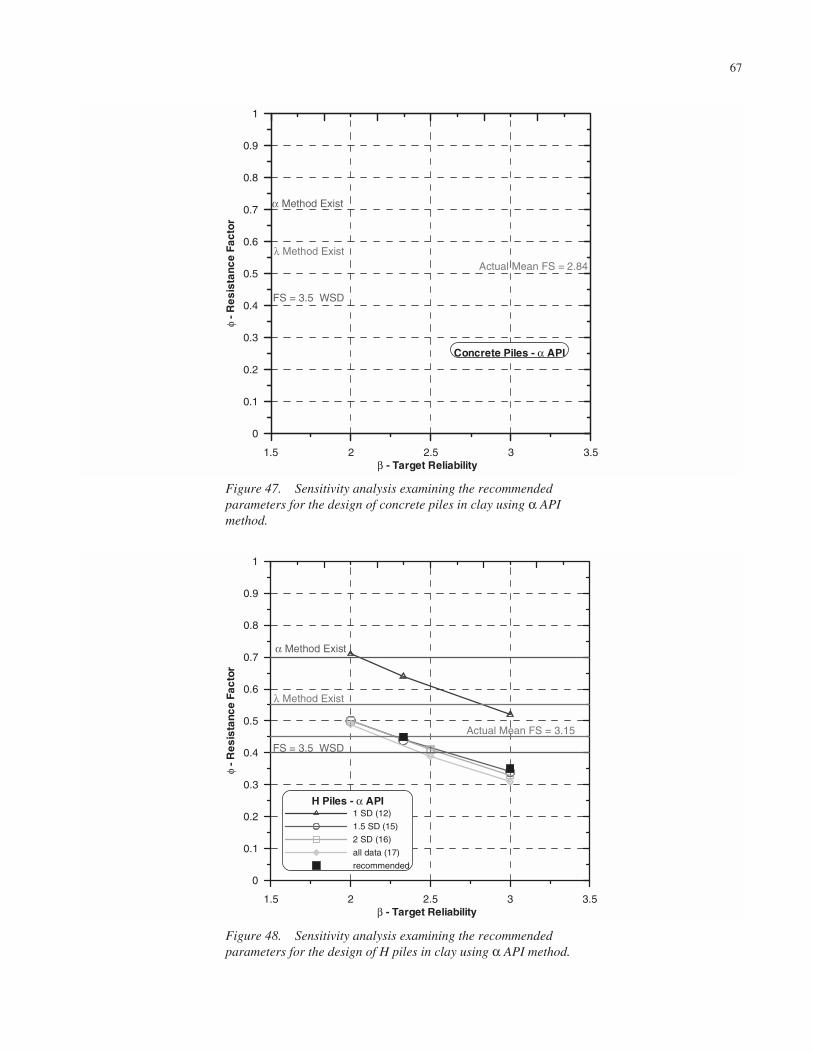
67
1.5 2 2.5 3 3.5β - Target Reliability
0
0.1
0.2
0.3
0.4
0.5
0.6
0.7
0.8
0.9
1
φ - R
esis
tanc
e Fa
ctor
Concrete Piles - α API
α Method Exist
λ Method ExistActual Mean FS = 2.84
FS = 3.5 WSD
1.5 2 2.5 3 3.5β - Target Reliability
0
0.1
0.2
0.3
0.4
0.5
0.6
0.7
0.8
0.9
1
φ - R
esis
tanc
e Fa
ctor
H Piles - α API1 SD (12)
1.5 SD (15)
2 SD (16)
all data (17)
recommended
α Method Exist
λ Method Exist
Actual Mean FS = 3.15
FS = 3.5 WSD
Figure 47. Sensitivity analysis examining the recommendedparameters for the design of concrete piles in clay using α APImethod.
Figure 48. Sensitivity analysis examining the recommendedparameters for the design of H piles in clay using α API method.

68
0.45
0.55
0.40
Nordlund
0.550.30.45H
0.55 0.30.30 Pipe
0.50 0.50.20 Concrete
SPT 97 β Meyerhof
Method Pile Type
Recommended φφφφ values for ββββ = 2.33
FS = 3.5WSD
0.45 λv SPT
0.55 λv CPT
Existing LRFD φφφφ values skin and end bearing
FHWA CPT mixed soil concrete piles φ = 0.50
No./Mean of prediction (data ±±±± 2 SD)
1.18*
0.94
1.48
1.02
74
19
19
36
Nordlund
1.34* 73 1.04* 74 0.75* 74 Total
1.35 18 0.78 19 0.81 18 H
1.58 19 1.18 20 0.94 20 Pipe
1.21 36 1.10 35 0.61 36 Concrete
SPT 97 βMeyerhof
MethodPile Type
Actual mean FS for driven piles in sand
Range: pipe piles SPT 97 = 1.58 x 3.5 = 5.53 Meyerhof PPC = 0.61 x 3.5 = 2.14
* - large variation between pile types
1.5 2 2.5 3 3.5β - Target Reliability
0
0.1
0.2
0.3
0.4
0.5
0.6
0.7
0.8
0.9
1
φ - R
esis
tanc
e Fa
ctor
Pipe Piles - β Method1 SD (13)
1.5 SD (18)
2 SD (20)
all data (20)
recommended
Actual Mean FS = 4.13
FS = 3.5 WSD
Figure 49. Data summary for parameter evaluation of driven piles in sand.
Figure 50. Sensitivity analysis examining the recommendedparameters for the design of pipe piles in sand using the β method.

69
1.5 2 2.5 3 3.5β - Target Reliability
0
0.1
0.2
0.3
0.4
0.5
0.6
0.7
0.8
0.9
1
φ - R
esis
tanc
e Fa
ctor
Concrete Piles - β Method1 SD (28)
1.5 SD (31)
2 SD (35)
all data (37)
recommended
Actual Mean FS = 3.85
FS = 3.5 WSD
1.5 2 2.5 3 3.5β - Target Reliability
0
0.1
0.2
0.3
0.4
0.5
0.6
0.7
0.8
0.9
1
φ - R
esis
tanc
e Fa
cto
r
H Piles - β Method1 SD (13)
1.5 SD (16)
2 SD (19)
all data (19)
recommended
Actual Mean FS = 2.73
FS = 3.5 WSD
Figure 51. Sensitivity analysis examining the recommendedparameters for the design of concrete piles in sand using the βmethod.
Figure 52. Sensitivity analysis examining the recommendedparameters for the design of H piles in sand using the β method.

70
Resistance factor
φ CAPWAP
General CAPWAP
BOR
CAPWAP EOD
AR > 350 BL ct. > 16 BP10cm
Energy Approach
EOD
FHWA Mod Gates
General
0.5 0.27 0 2.70 1.56 10.420.4 0 0 0 0 3.13
0.33 0 0 0 0 0.78
# of cases used 377 162 37 128 384
TABLE 31 Calculated probability of failure [p = (%)] based on direct utilizationof database PD/LT 2000 for selected prediction methods
71
CHAPTER 4
CONCLUSIONS AND SUGGESTED RESEARCH
4.1 CONCLUSIONS
The data and analyses presented in this report lead to thefollowing major conclusions:
1. The compilation of large databases allows for the quan-titative assessment of pile capacity evaluation methodsduring both design and construction. In addition, data-bases (combined with the application of mechanicsprinciples) allow the determination of the controllingparameters of capacity evaluation methods that requirecalibration. Databases are essential therefore for theexamination of any design methodology and henceenable the testing of the factors of safety used by WSD(i.e., their validity and effect on costs) and the devel-opment of other methodologies, such as LRFD.
2. LRFD facilitates a design methodology that is moresuitable for geotechnical applications than WSD. Theability to determine design factors while quantifyingthe significance of their outcome is a powerful tool inengineering. The development of load and resistancefactors utilizing reliability-based calibration and data-bases is a major necessary step toward objective quan-tification of the LRFD parameters. More so, it allows ameaningful utilization of the LRFD principles (in con-trast to parameter fitting to WSD) and sets a base forfuture developments that will further rationalize designand lead to more economical construction.
3. The findings presented are the first of their kind in the development of resistance factors for LRFD designmethodologies in geotechnical engineering. A review ofthe recommended resistance factors must be compatiblewith the fundamental principle of the methodology, i.e.engineering design with a consistent level of reliability.Existing LRFD codes worldwide were developed, byand large, to be compatible with previous WSD parame-ters based on different concepts. While radical changescannot be expected in construction practices, a shift inboth directions (more and less conservative dependingon the specifics) should be expected and accepted whenadopting a true LRFD design.
4.2 SUGGESTED RESEARCH—KNOWLEDGE-BASED DESIGNS
4.2.1 Statement of Problem
Variability in the parameters used in the design, site con-ditions, construction quality, and previous experience are allimportant factors. The present study bypassed some of thedifficulties by calibrating specific design methods and corre-lations as a unit. A more complete design process based onLRFD can recognize the contribution of different factors—such as subsurface variability, site-specific technology, andprevious experience—as well as amount and type of testingduring construction. A framework for such an approach ispresented here; further development, however, will requireadditional databases, e.g., for the correlation between soilparameters and field tests, as well as subjective judgments.
4.2.2 Framework for LRFD Design for Deep Foundations
In order to fully exploit the potential of the LRFD method-ology for geotechnical purposes the aforementioned issuesmust be addressed. Many of the affecting factors are in factbeing considered in the design (e.g., previous experience) butneed a framework to allow future progress. A proposed solu-tion is to establish knowledge-based factors for both thedesign and the construction (independent) capacity evaluationmethods. These factors can be accounted for by a modifyingconstant ξ to be multiplied by the resistance factor.
ξφ R > γL (40)
Where:
ξ = ξ1 ξ2 ξ3 ξ4 ≤ ξlimit
ξ1 = factor adjusting for the variability of site conditionsξ2 = factor adjusting for the quality of soil parameter
estimatesξ3 = factor adjusting for construction quality controlξ4 = factor adjusting for previous site or construction
experience

ξlimit = an upper limit on the factor that will be determinedfrom computing the components of ξ (and judg-ment). The limit should have some real value largerthan 1.0, such as 1.10.
A short description of the knowledge-based factors follows.ξ1 applies to the spatial variation of soil properties, strati-
fication across a site, and the extent to which that variationhas been categorized by the subsurface investigation pro-gram. The factor is relevant for deep foundations capacityevaluation during both design and construction. Low valuesmean that the site is more erratic than normal or that littleexploration and testing has been done. Average values reflectnormally variable soil conditions adequately investigated.High values mean that the site is more uniform than normaland that an extensive program of boring and testing has beenconducted. The extent of exploration can be evaluated vianumber of borings per substructure unit.
ξ2 applies only to deep foundations capacity methodsemploying calculations based on soil parameters. This factoraccounts for the manner in which soil parameters are estimatedfrom field and laboratory test data and the exactness of thoseestimates. Low values mean that the correlation between soilparameters and the measurements they are based upon is poor(e.g., when estimating undrained shear strength of soft to
72
medium clay from SPT values), and thus the confidence in theaccuracy of the soil parameter values is low. Average valuesreflect normally variable soil conditions adequately inves-tigated. High values mean that the correlation is good (e.g.,when parameters are estimated based on laboratory test ofundisturbed samples or direct in situ testing like a field vanetest), and thus the confidence in parameter values is high.
ξ3 applies to the extent of measures taken to control con-struction quality and testing the integrity and capacity of theconstructed deep foundations. Low values mean that fewmeasures are to control construction quality; and no static,dynamic, or integrity testing results are available. High val-ues mean that extensive measures are taken to control con-struction quality, and multiple pile testing results are avail-able (e.g., integrity and capacity of drilled shafts, static anddynamic tests of driven piles). The high quality control alsorelates to the number of tested deep foundations as a ratio ofthe number of piles installed per substructure.
ξ4 is to be used during the design to account for previousexperience accumulated either on a specific construction siteor from a specific construction technology. Low values areused if no previous experience is known at the site and a newunfamiliar construction technology is used. High values meanthat previous deep foundation testing results similar to theone designed (type and installation) are available.
73
BIBLIOGRAPHY*
AASHTO. 1994. LRFD Bridge and Construction Specifications.AASHTO, Washington, DC.
AASHTO. 1996/2000. LRFD Bridge Design Specifications: 2ndLRFD Edition—2000 Interim Revisions. AASHTO, Washing-ton, DC.
AASHTO. 1997. Standard Specifications for Highway Bridges: 16thEdition (1996 with 1997 interims). AASHTO, Washington, DC.
AASHTO. 2001. LRFD Bridge Design Specifications. AASHTO,Washington, DC.
American Concrete Institute (ACI). 1995, Building Code Require-ments for Reinforced Concrete. American Concrete Institute,Detroit, MI.
American Institute of Steel Construction (AISC). 1994. Load andResistance Factor Design. Manual of Steel Construction, Amer-ican Institute of Steel Construction, Chicago, IL.
American Petroleum Institute (API). 1989. Draft RecommendedPractice for Planning, Designing and Constructing Fixed OffshorePlatforms—Load and Resistance Factor Design. API RP2A-LRFD. American Petroleum Institute, Dallas, TX.
ASCE. 1993. Minimum Design Loads for Buildings and Other Struc-tures ASCE 7-93. (Formerly ANSI A58.1). ASCE, Reston, VA.
AUSTROADS. 1992. AUSTROADS Bridge Design Code. NationalOffice, AUSTROADS, Surry Hills, NSW, Australia.
Ayyub, B.M. 1999. Cost-Benefit Analysis of Risk-Informed Design ofStructural Systems. American Society of Mechanical Engineers,the Research Committee on Risk Technology, Washington, DC.
Ayyub, B., and Assakkaf, I. 1999. LRFD Rules for Naval SurfaceShip Structures: Reliability-Based Load and Resistance FactorDesign Rules. Naval Surface Warfare Center, Carderock Divi-sion, U.S. Navy.
Ayyub, B., Assakkaf, I., and Atua, K. 1998a. Development of LRFDRules for Naval Surface Ship Structures: Reliability-Based Loadand Resistance Factor Design Rules, Part III—Stiffened andGross Panels. Naval Surface Warfare Center, Carderock Divi-sion, U.S. Navy.
Ayyub, B., Assakkaf, I., and Atua, K. 2000. Reliability-Based Loadand Resistance Factor Design (LRFD) of Hull Girders for SurfaceShips. Naval Engineers Journal, Vol. 112, No. 4, July 2000, pp.279–296.
Ayyub, B., Assakkaf, I., Atua, K., Engle, A., Hess, P., Karaszewski,Z., Kihl, D., Melton, W., Sielski, R., Sieve, M., Waldman, J., andWhite, G. 1998b. Reliability-based Design of Ship Structures:Current Practice and Emerging Technologies. T&R Report R-53,Society of Naval Architects and Marine Engineers.
Ayyub, B., and McCuen, R. 1997. Probability, Statistics and Reli-ability for Engineers. CRC Press, FL.
Baecher, G. 2001. Contribution to a progress research report as partof Project NCHRP 24-17, LRFD Deep Foundations Design,unpublished document.
Barker, R., Duncan, J., Rojiani, K., Ooi, P., Tan, C., and Kim, S.1991. NCHRP Report 343: Manuals for the Design of BridgeFoundations. TRB, National Research Council, Washington, DC.
Becker, D. 1996. Eighteenth Canadian Geotechnical Colloquium:Limit States Design for Foundations. Part I. An overview of the
foundation design process. Canadian Geotechnical Journal, Vol.33, No. 6, December, pp. 956–983.
Benjamin, J. R., and Cornell, C. A. 1970, Probability, Statistics,and Decision for Civil Engineers. McGraw-Hill, New York.
Bermingham, P., and White, J. 1995. Pyrotechnics and the AccuratePrediction of Statnamic Peak Loading and Fuel Charge Size.Proceedings First International Statnamic Seminar, September27–30, Vancouver, BC, Canada, pp. 1–12.
Bowles, J. 1996. Foundation Analysis and Design. McGraw-Hill,New York.
Brooms, B. 1964a. “Lateral Resistance of Piles in Cohesive Soils.”Journal of the Soil Mechanics and Foundations Division, ASCE,Vol. SM2, March, pp. 27–63.
Brooms, B. 1964b. “Lateral Resistance of Piles in CohesionlessSoils.” Journal of the Soil Mechanics and Foundations Division,ASCE, Vol. SM3, May, pp.123–156.
Butler, H.D., and Hoy, H.E. 1977. Users Manual for the TexasQuick-Load Method for Foundation Load Testing. FHWA-IP-77-8. FHWA, Office of Development, Washington, DC.
Canadian Geotechnical Society. 1992. Canadian Foundation Engi-neering Manual, 3rd Edition. Bi-Tech Publishers, Ltd., Rich-mond, British Columbia, Canada.
Carter, J. P., and Kulhawy, F. H. 1988. Analysis and Design ofFoundations Socketed into Rock. Electric Power Research Insti-tute, Report Number EPRI EL-5918.
Construction Industry Research and Information Association(CIRIA). 1977. Rationalization of Safety and Serviceability Fac-tors in Structural Codes: CIRIA Report 63. Construction Indus-try Research and Information Association, SWIP 3AU, Report63, London, England.
Chellis, R.D. 1961. Pile Foundation, 2nd ed. McGraw Hill, NY.Davisson, M. 1972. High Capacity Piles. In Proceedings, Soil
Mechanics Lecture Series on Innovations in Foundation Con-struction, ASCE, Illinois Section, Chicago, IL, pp. 81–112.
DeBeer, E. 1970. Proefondervindellijke bijdrage tot de studie vanhet grandsdraagvermogen van zand onder funderinger op staal.English version. Geotechnique, Vol. 20, No. 4, pp. 387–411.
DiMaggio, J., Saad, T., Allen, T., Passe, P., Goble, G., Christopher,B., DiMillio, A., Person, G., and Shike, T. 1998. FHWA SummaryReport of the Geotechnical Engineering Study Tour (GEST).FHWA International Technology Scanning Program, Decem-ber, FHWA.
DiMillio, A. 1999. A Quarter Century of Geotechnical Research.FHWA-RD-98-139, FHWA.
Ellingwood, B., Galambos, T., MacGregor, J., and Cornell C. 1980.Development of a Probability-Based Load Criterion for Ameri-can National A58. National Bureau of Standards Publication 577.Washington, DC.
Ellingwood, B., Galambos, T. 1982. Probability-Based Criteria forStructural Design. Structural Safety, Vol.1, pp. 15–26.
Ellingwood, B., Galambos, T., MacGregor, J., and Cornell, C.1982a. Probability Based Load Criteria—Assessment of CurrentDesign Practices. Journal of the Structural Division, ASCE, Vol.108, No. ST5, pp. 959–977.
Ellingwood, B., Galambos, T., MacGregor, J., and Cornell, C.1982b. Probability Based Load Criteria—Load Factors and Load*Bibliographic material not verified by TRB.

Combinations. Journal of the Structural Division, ASCE, Vol.108, ST5, pp. 978–997.
Esrig, M. I., and Kirby, R. C. 1979. Soil Capacity for Supporting DeepFoundation Members in Clay. ASTM STP. No. 670, pp. 27–63.
Eurocode 7. 1997. Geotechnical Design—Part I: General Rules. Euro-pean Committee for Standardization, Central Secretariat, Brussels.
FHWA. 1988. Geotechnical Guideline No. 13. FHWA, 37 pp.Fragaszy, R., Higgins, J., and Lawton, E. 1985. Development of
Guidelines for Construction Control of Pile Driving and Estima-tion of Pile Capacity: Phase I. Washington DOT Report WA/RD-68.1, Olympia, Washington, 83 pp.
Freudenthal, A. 1947. Safety of Structures. Transactions of theASCE. Vol. 112, pp. 125–180.
Galambos, T., and Ravindra, M. 1978. Properties of Steel for Usein LRFD. Journal of Structural Engineering, Vol. 104, No. 9, pp.1459–1468.
Gates, M., 1957. Empirical Formula for Predicting Pile BearingCapacity. Civil Engineering, Vol. 27, No. 3, pp. 65–66.
Geosciences Testing and Research, Inc. 1997. Dynamic Pile TestingReport, Central Artery/Tunnel Project C07D2, I-90/Airport Inter-change Arrivals Tunnel—Phase I, East Boston, Massachusetts.Geosciences Testing and Research, Inc. North Chelmsford, MA.
Geosciences Testing and Research, Inc. (GTR). 1998. Dynamic PileTesting Report, Central Artery/Tunnel Project C07D2, I-90/Airport Interchange Toll Plaza, East Boston, Massachusetts.Geosciences Testing and Research, Inc., North Chelmsford, MA.
Goble, G. 1999. NCHRP Synthesis of Highway Practice 276: Geo-technical Related Development and Implementation of Loadand Resistance Factor Design (LRFD) Methods. TRB, NationalResearch Council, Washington, DC.
Goble, G., Likens, G., and Rausche, F. 1970. Dynamic Studies onthe Bearing Capacity of Piles—Phase III. Report No. 48. Divi-sion of Solid Mechanics, Structures, and Mechanical Design.Case Western Reserve University.
Goble, G., and Rausche, F. 1976. Wave Equation Analysis of PileDriving-WEAP Program. Vol. 1–4. FHWA #IP-76-14.1 through#IP-76-14.4.
GRL, Inc. 1999. Pile-Driving Analyzer, PAK Users Manual. Goble,Rausche, Likins and Associates, Inc.
Grant, E., and Leavenworth, R. 1996. Statistical quality control. 7thed., McGraw-Hill, New York, NY, 1996. pp. 764.
Hajduk, E., Paikowsky, S., Hölscher, P., and Barends, F. 2000. Accel-erations of a Driven Pile and the Surrounding Soil. Proceedings ofthe 6th International Conference on the Applications of Stress-Wave Theory to Piles, S. Niyama, and J. Beim eds., September11–13, São Paulo, Brazil, Balkema, Rotterdam-the Netherlands,pp. 541–548.
Hamilton, J., and Murff, J. 1992. Selection of LRFD ResistanceFactors for Pile Foundation Design. American Society of CivilEngineers Structures Congress, April 13–15, San Antonio, Texas,Proceedings Structures Congress ’92, ASCE.
Hannigan, P., Goble, G., Thendean, G., Likins, G., and Rausche, F.1995. Design and Construction of Driven Pile Foundation.FHWA, Washington, DC.
Hannigan, R., Goble, G., Thendean, G., Likins, G., and Rausche, F.1996. Design and Construction of Driven Piles Foundations—Volume II (Working Draft). U.S. DOT, FHWA. Washington, DC.
Hansen, B. 1953. Earth Pressure Calculation. Danish TechnicalPress, Copenhagen, Denmark.
Hansen, B. 1956. Limit Design and Safety Factors in Soil Mechan-ics. Bulletin No. 1, Danish Geotechnical Institute, Copenhagen,Denmark.
74
Hansen, B. 1966. Code of Practice for Foundation Engineering.Bulletin No. 22, Danish Geotechnical Institute, Copenhagen,Denmark.
Hasofer, A. M., and Lind, N. C. 1974. An Exact and Invariant First-Order Reliability Format. Journal of Engineering Mechanics,Vol. 100. No. EM1, pp. 111–121.
Hölscher, P. 1995. Dynamical Response of Saturated and Dry Soils.Delft University Press, Delft, The Netherlands.
Hölscher, P., and Barends, F. 1996. In-situ Measurement of Soil-Motion near the Toe of a Dynamically Loaded Pile. In Proceed-ings, 5th International Conference of the Application of Stress-Wave Theory to Piles, September 11–13, 1996 Orlando, FL (F.C.Townsend, M. Hussein, and M. McVay, eds.), pp. 26–36.
Japanese Geotechnical Society. 1998. Foundation Design Stan-dards in the World—Toward Performed-Based Design. ResearchCommittee on Present & Future of Japanese Foundation Designand Soil Investigation in View of International Equivalency.
Kulhawy, F., and Phoon, K. 1996. Engineering Judgment in theevolution from Deterministic to Reliability-Based FoundationDesign. Proceedings of the 1996 Conference on Uncertainty inthe Geologic Environment, UNCERTAINTY’96. Part 1 (of 2),July 31–Aug. 31, Madison, WI, ASCE, NY, pp. 29–48.
Kulhawy, F., and Mayne, P. 1990. Manual on Estimating of SoilProperties for Foundation Design. Electric Power Research Insti-tute, Palo Alto, CA.
Kuo, C., McVay, M., and Birgisson, M. 2002. Calibration of Loadand Resistance Factor Design: Resistance Factors for DrilledShaft Design, TRB, Transportation Research Record, No. 1808,pp.108–111, Annual Meeting, January 13–17, Washington, DC.
Lai, P., and Graham, K. 1995. Static Pile Bearing Analysis Program.SPT94. http://www.dot.state.fl.us/structures/manuals/spt94.zip
Long, J.; Bozkurt, D.; Kerrigan, J.; Wysockey, M. 1999. Value ofMethods for Predicting Axial Pile Capacity. TRB TransportationResearch Record No. 1663, pp. 57–63, 76th Annual Meeting,January, Washington, DC.
Madsen, H.O., Krenk, S. and Lind, N.C. 1986. Methods of Struc-tural Safety. Prentice Hall, Englewood Cliffs, NJ.
Mansour, A.E., Wirsching, P.H., Ayyub, B.M., and White, G.J.1994. Probability Based Ship Design Implementation of DesignGuidelines for Ships, Ship Structures Committee Draft Report.U.S. Coast Guard, Washington, DC.
Massachusetts. Code of Massachusetts Regulations (CMR). StateBuilding Code—780, 1997. Article 12, section 1214.3.1, DrivingFormula, CMR 5th edition.
Massachusetts Highway Department. 1988. Standard Specificationsfor Highways and Bridges. Massachusetts Highway Department.
McVay, M., Birgisson, B., Nguyen, T., and Kuo, C. 2002. Uncer-tainty in LRFD phi, φ, Factors for Driven Prestressed ConcretePiles, TRB, Transportation Research Record 1808, pp. 99–107,Annual Meeting, January 13–17, Washington, DC.
McVay, M., Birgisson, B., Zhang, L., Perez., A, and Putcha, S.2000. Load and Resistance Factor Design (LRFD) for DrivenPiles Using Dynamic Methods—A Florida Perspective. Geo-technical Testing Journal, Vol. 23, No. 1, pp. 55–66.
McVay, M., and Townsend, F. 1989. Short Course/WorkshopGuide for PC Software Support for Design and Analysis of Deepand Shallow Foundations from In-situ Tests (or PL-AID Man-ual). University of Florida, Gainesville, Florida.
Melchers, R. E. 1987. Structural Reliability Analysis and Predic-tion. Ellis Horwood Limited, UK.
Meyerhof, G. 1970. Safety Factors in Soil Mechanics. CanadianGeotechnical Journal, Vol. 7, No. 4, pp. 349–355.
Meyerhof, G. 1976. Bearing Capacity And Settlement Of PileFoundations. American Society of Civil Engineers, Journal ofthe Geotechnical Engineering Division, Vol. 102, No. 3, March,pp. 195–228.
Meyerhof, G. 1994. Evolution of Safety Factors and GeotechnicalLimit State Design. Second Spencer J. Buchanan Lecture, TexasA and M University, Nov. 4, pp. 32.
Middendorp, P., and Bielefeld, M. 1995. Statnamic Load Testingand the Influence of Stress Wave Phenomena. Proceedings of theFirst International Statnamic Seminar, Vancouver, BC, Canada,September 27–30, pp. 207–220.
Middendorp, P., and van Weel, P. 1986. Application of Character-istic Stress-Wave Method in Offshore Practice. Proceedings ofNumerical Methods in Offshore Piling: 3rd International Con-ference, Nantes, May 21–22, Editions Technip.
Moses, F. 1985. Implementation of a Reliability-Based API RP2AFormat, Final Report. API PRAC 83-22. American PetroleumInstitute, Dallas, TX.
Moses, F. 1986. Development of Preliminary Load and ResistanceFactor Design Document for Fixed Offshore Platforms, FinalReport. API-PRAC 95-22, American Petroleum Institute, Dal-las, TX.
Moses, F., and Verma, D. 1987. NCHRP Report 301: Load Capac-ity Evaluation of Existing Bridges. TRB, Washington, DC.
National Research Council. 1995. Probabilistic Methods in Geo-technical Engineering. National Academies Press, Washington,DC, pp. 96.
National Research Council of Canada. 1977. National Building Codeof Canada. Ottawa, Canada.
Nordic Committee on Building Regulations. 1978. Recommenda-tions for Loading and Safety Regulations for Structural Design.Nordic Committee for Safety of Structures, NKB Report No. 36.Copenhagen, Denmark.
Nordlund, R. L. 1963. Bearing Capacity of Piles in CohesionlessSoils. Journal of Soil Mechanics and Foundation Engineering,JSMFE, Vol. 89, SM 3, pp 1–36.
Nottingham, L., and Schmertmann, J. 1975. An Investigation of PileCapacity Design Procedures. Final Report D629 to FloridaDepartment of Transportation, Department of Civil Engineering,University of Florida, pp 159.
Nowak, A. 1999. NCHRP Report 368: Calibration of LRFD BridgeDesign Code. TRB, Washington, DC.
Olsen, R., and Flaate, K. 1967. Pile Driving Formulas for FrictionPiles in Sand. Journal of Soil Mechanics and Foundation Engi-neering, JSMFE, Vol. 93, SM6, Nov. 1967, 279–297.
O’Neill, M. 1995. LRFD Factors for Deep Foundations throughDirect Experimentation. In Proceedings of US/Taiwan Geotech-nical Engineering Collaboration Workshop. Sponsored by theNational Science Foundation (USA) and the National ScienceCouncil (Taiwan, ROC), A.B. Huang, Y.S. Fang, P.W. Mayne,and S.G. Paikowsky eds., Taipei, January 9–11, pp. 100–114.
O’Neill, M., and Reese, L. 1999. Drilled Shafts: Construction Pro-cedures and Design Methods, Volume II Chapters 9–19, Appen-dices. U.S. DOT, FHWA, Washington, DC.
O’Neill, M., Townsend, F., Hassan, K., Buller, A., and Chang, P.1996. Load Transfer for Drilled Shafts in Intermediate Geoma-terials, FHWA-RD-95-172, FHWA.
Ontario Ministry of Transportation and Communication. 1992.Ontario Highway Bridge Design Code and Commentary. 3rd ed.
75
Orr, T. 2002. Eurocode 7— A Code for Harmonized GeotechnicalDesign. Proceedings of the International Workshop on Founda-tion Design Codes and Soil Investigation in View of InternationalHarmonization and Performance Based Design, IWS Kamakura2002, Tokyo, Japan, April 10–12, Y. Honjo, O. Kusakabe, K.Matsui, M. Kouda, and G. Pokharel eds., Balkema, the Nether-lands, pp. 3–15.
Orr, T., and Farrell, E. 1999. Geotechnical Design to Eurocode 7.Springer-Verlag, UK, pp. 175
Osterberg, J. 1992. The Osterberg Cell for Load Testing DrilledShafts And Driven Piles. FHWA Report SA-94-035, Washing-ton, DC.
Paikowsky, S. 1982. Use of Dynamic Measurements to Predict PileCapacity Under Local Conditions. M.Sc. Thesis, Dept. of CivilEngineering Technion-Israel Institute of Technology, Haifa, Israel.
Paikowsky, S. 1984. Use of Dynamic Measurements for Pile Analy-sis. Including PDAP-Pile-Driving Analysis Program. GZA Inc.,Newton, Massachusetts.
Paikowsky, S. 1995. Using Dynamic Measurements for the Capac-ity Evaluation of Driven Piles. Civil Engineering Practice, Jour-nal of the Boston Society of Civil Engineers Section/ASCE. Vol.10, No. 2, pp. 61–76.
Paikowsky, S., and Chernauskas, L. 1992. Energy Approach forCapacity Evaluation of Driven Piles. Proceedings of the 4thInternational Conference on the Application of Stress-Wave The-ory to Piles, F.B. Barends ed., September 21–24, The Hague, TheNetherlands, pp. 595–601.
Paikowsky, S., and Chernauskas, L. 1996. Soil Inertia and the Useof Pseudo Viscous Damping Parameters. Proceedings of the 5thInternational Conference on the Application of Stress-Wave The-ory to Piles, F.C. Townsend, M. Hussein, and M.C. McVay eds.,September 11–13, Orlando, FL, pp. 203–216.
Paikowsky, S., and Hajduk, E. 1999. Design and Construction of anInstrumented Test Pile Cluster: Research Report submitted to theMassachusetts Highway Department, September, 1999. Univer-sity of Massachusetts—Lowell, MA.
Paikowsky, S., and Hajduk, E. 2000. Theoretical Evaluation and FullScale Field Testing Examination of Pile Capacity Gain with Time:Research Report submitted to the Massachusetts Highway Depart-ment, December, University of Massachusetts—Lowell, MA.
Paikowsky, S., and Hart, L. 2000. Development and Field Testingof Multiple Deployment Model Pile (MDMP): Research Reportto be submitted to the Federal Highway Administration, April,2000. FHWA-RD-99-194. FHWA.
Paikowsky, S., and LaBelle, V. 1994. Examination of the EnergyApproach for Capacity Evaluation of Driven Piles. Proceedingsof the International Conference on Design and Construction ofDeep Foundations, December 6–8, Orlando, FL. FHWA, Vol. II,pp. 1133–1149.
Paikowsky, S., LaBelle, V., and Hourani, N. 1996. Dynamic Analy-ses and Time Dependent Pile Capacity. Proceedings of the 5thInternational Conference on the Application of Stress-Wave The-ory to Piles, F.C. Townsend, M. Hussein, and M.C. McVay eds.,September 11–13, Orlando, FL, pp. 325–339.
Paikowsky, S., LaBelle, V., and Mynampaty, R. 1995. Static andDynamic Time Dependent Pile Behavior: Research Report sub-mitted to the Massachusetts Highway Department, November,University of Massachusetts—Lowell, MA.
Paikowsky, S., Operstein, V., and Bachand, M. 1999. ExpressMethod of Pile Testing by Static Cyclic Loading. Research Reportsubmitted to the Massachusetts Highway Department, October,University of Massachusetts—Lowell, MA.
Paikowsky, S., Regan, J., and McDonnell, J. 1994. A SimplifiedField Method for Capacity Evaluation of Driven Piles. FHWA-RD-94-042, FHWA.
Paikowsky, S., and Stenersen, K. 2000. The Performance of theDynamic Methods, their Controlling Parameters and Deep Foun-dation Specifications. Keynote lecture in Stress Wave 2000, Pro-ceedings of the Sixth International Conference on the Applicationof Stress-Wave Theory to Piles, S. Niyama, and J. Beim eds., Sep-tember 12, São Paulo, Brazil, Balkema, Rotterdam—the Nether-lands, pp. 281–304.
Paikowsky, S., and Whitman, R. 1990. The Effect of Plugging onPile Performance and Design. Canadian Geotechnical Journal,Vol. 27, No. 4, pp. 429–440.
Paikowsky, S., Whitman, R., and Baligh, M. 1989. A New Look atthe Phenomenon of Offshore Pile Plugging. Marine Geotechnol-ogy, Vol. 8, No. 3, pp. 213–230.
Payer, H., Huppmann, H., Jochum, C., Madsen, H., Nittinger, K.,Shibata, H., Wild, W., and Wingender, H. 1994. Plenary PanelDiscussion on How Safe is Safe Enough? Proceedings of the 6thInternational Conference on Structural Safety and Reliability,G.I. Schueller, M. Shinozuka and J.T.P. Yao eds., ICOSSAR ‘93,Innsbruck, August 9–13, Balkema, Rotterdam, The Netherlands,pp. 57–74.
Phoon, K.K., and Kulhawy, F.H. 1996. On Quantifying InherentSoil Variability. Uncertainty in the Geologic Environment: fromTheory to Practice Proceedings of Uncertainty ’96, C.D. Shack-elford, P.P. Nelson, and M.J.S. Roth eds., Madison, WI, July31–August 3, ASCE, New York, pp. 326–340.
Phoon, K., Kulhawy, F. and Grigoriu, M. 1995. Reliability-BasedDesign of Foundations for Transmission Line Structures. ReportTR-105000. Electrical Power Research Institute (EPRI), PaloAlto, Texas.
Rausche, F. 2000. Personal communication. February 2000.Rausche, F., Goble, G., and Likens, G. 1975. Bearing Capacity of
Piles from Dynamic Measurements, Final Report. Ohio DOT-05-75. Ohio Department of Transportation.
Rausche, F., Thendean, F., Abou-matar, H., Likins, G., and Goble, G.1997. Determination of Pile Driveability and Capacity from Pene-tration Tests. Vol. 1–3, Final Report. FHWA-RD-96-179, FHWA.
Reese, L. C., and O’Neill M. W. 1988. Drilled Shaft: ConstructionProcedures and Design Methods. FHWA-HI-88-042, FHWA.
Reese, L.C., Wang, S.C., and Arrellaga, J. 1998. APILE Plus 3.0Manual. EnSoft, Inc. Austin, TX.
Reese, L. C., and Wright S. J. 1977. Construction Procedures andDesign for Axial Loading, Drilled Shaft Manual HDV-22.
Rosenblueth, E., and Esteva, L. 1972. Reliability Basis for SomeMexican Codes. ACI Publication SP-31. American Concrete Insti-tute, Detroit, MI.
Siu, W., Parimi, S., and Lind, N. 1975. Practical Approach to CodeCalibration. Journal of the Structural Division, Vol. 101, No.ST7, pp. 1469–1480.
Smith, E. 1960. Pile Driving Analysis by the Wave Equation. Jour-nal of Soil Mechanics and Foundations, ASCE, Vol. 86, No.SM4, August 1960, pp. 35–61.
Standards Association of Australia. 1995. Australian Standards,Piling-Design and Installation. Standards Association of Aus-tralia, Homebush, NSW, Australia.
Tang, W. 1993. Recent Developments in Geotechnical Reliability.Proceedings of the Conference on Probabilistic Methods in Geo-technical Engineering Li, K., and Lo, S-C. eds., Canberra, Aus-
76
tralia, February 10–12, Balkema, Rotterdam, The Netherlands,pp. 3–28.
Tang Q., Drumm, E.C., and Bennett, R.M. 1994. Response toDrilled Shaft Foundations in Karst During Construction Loading,Proceedings of the International Conference on Design and Con-struction of Deep Foundations, December 6–8, Orlando, FL,FHWA, Vol. III, pp. 1296–1309.
Tang, W., Woodford, D., and Pelletier, J. 1990. Performance Reli-ability of Offshore Piles. Proceedings of the 22nd Annual Off-shore Technology Conference. May 7–10, Houston, TX, PaperNo. OTC 6379, Offshore Technology Conference, Richardson,TX, Vol. 3, p. 299–308.
Terzaghi, K. 1942. Discussion of the Progress Report of the Com-mittee on the Bearing Value of Pile Foundations. Proceedings,ASCE. Vol. 68, pp. 311–323.
Terzaghi, K., and Peck, R.B. 1967. Soil Mechanics in EngineeringPractice. Wiley.
Thoft-Christensen, P., and Baker, M. 1982. Structural ReliabilityTheory and Its Application. Springer-Verlag, New York.
Tomlinson, M.J., 1986. Foundation Design and Construction.Longman Scientific and Technical, Essex, England.
Tomlinson, M.J. 1995. Foundation Design and Construction. 6thEdition. Longman Scientific and Technical, Essex, England.
Trautmann, C., and Kulhawy, F. 1996. “Estimation of In-situ TestUncertainty.” Uncertainty in Geological Environment: FromTheory to Practice, pp. 269–86.
U.S. Army Corps of Engineers. 1992. Bearing Capacity of Soil,Technical Engineering and Design Guides. Adapted by ASCE—2000, No.7, EM 1110-1-1905. ASCE Press, New York.
Vijayvergiya, V.N., and Focht Jr., J.A. 1972. A New Way to Pre-dict Capacity of Piles In Clay. Proceedings of the 4th Annual Off-shore Technology Conference, Houston, TX, Offshore Technol-ogy Conference, Richardson, TX, Vol. 2, pp. 856–874.
Wellington, A. 1892. Discussion of “The Iron Wharf at Fort Mon-roe, Va. By J.B. Cuncklee.” Transactions, ASCE Vol. 27, paperNo. 543, Aug. 1892, pp. 129–137.
Whitman, R. 1984. Evaluating Calculated Risk in GeotechnicalEngineering. The Seventeenth Terzaghi Lecture. Journal of Geo-technical Engineering, Vol. 110, No. 2, pp. 145–188.
Wirsching, P. H. 1984. Fatigue Reliability for Offshore Struc-tures. Journal of Structural Engineering, Vol. 110, No. 10, pp2340–56.
Withiam, J., Voytko, E., Barker, R., Duncan, M., Kelly, B., Musser,S., and Elias, V. 1998. Load and Resistance Factor Design (LRFD)of Highway Bridge Substructures. FHWA HI-98-032. FHWA.
Wu, T., Tang, W., Sangrey, D., and Baecher, G., 1989. Reliabilityof Offshore Foundations—State of the Art. Journal of Geotech-nical Engineering, Vol. 115, No. 2, pp. 157–178.
Zeitlen, J.G., and Paikowsky, S.G. Nov. 1982. “New Design Cor-relations for Piles in Sand.” Discussion in ASCE Journal of GE,108, No. GT11, pp. 1515–1518.
Zhang, L., Silva-Tulla, F., and Grismala, R. 2002. Ultimate Resis-tance of Laterally Loaded Piles in Cohesionless Soils, Proceed-ings of the International Deep Foundations Congress 2002: AnInternational Perspective on Theory, Design, Construction, andPerformance. February 14–16, 2002 Orlando, Florida, Geotech-nical Special Publication No. 116, ASCE, pp.1364–1375.
Zhang, L., Tang, W., and Ng, C. 2001. Reliability of Axially LoadedDriven Pile Groups. Journal of Geotechnical and Geoenviron-mental Engineering, Vol. 127, No. 12, pp. 1051–1060.

A-1
APPENDIXES
Appendixes A through D are published on the accompanying CD (CRP-CD-39). The appendixes and their authorship are as follows:
• Appendix A: Surveys—State of Practice Design and Construction (Ching L. Kuo, Bjorn Birgisson, Michael McVay, andSamuel G. Paikowsky)
• Appendix B: Load and Resistance Factor Design (LRFD) for Dynamic Analyses of Driven Piles (Samuel G. Paikowskyand Kirk L. Stenersen)
• Appendix C: Static Analyses of Driven Piles and Drilled Shafts (Ching L. Kuo, Bjorn Birgisson, Michael McVay, andSamuel G. Paikowsky)
• Appendix D: Design Examples (Ching L. Kuo, Samuel G. Paikowsky, Kirk Stenersen, Roiy Guy, Bjorn Birgisson, andMichael McVay)

Abbreviations used without definitions in TRB publications:
AASHO American Association of State Highway OfficialsAASHTO American Association of State Highway and Transportation OfficialsAPTA American Public Transportation AssociationASCE American Society of Civil EngineersASME American Society of Mechanical EngineersASTM American Society for Testing and MaterialsATA American Trucking AssociationsCTAA Community Transportation Association of AmericaCTBSSP Commercial Truck and Bus Safety Synthesis ProgramFAA Federal Aviation AdministrationFHWA Federal Highway AdministrationFMCSA Federal Motor Carrier Safety AdministrationFRA Federal Railroad AdministrationFTA Federal Transit AdministrationIEEE Institute of Electrical and Electronics EngineersITE Institute of Transportation EngineersNCHRP National Cooperative Highway Research ProgramNCTRP National Cooperative Transit Research and Development ProgramNHTSA National Highway Traffic Safety AdministrationNTSB National Transportation Safety BoardSAE Society of Automotive EngineersTCRP Transit Cooperative Research ProgramTRB Transportation Research BoardU.S.DOT United States Department of Transportation


![SUMMARY CHANGES FOR NCHRP REPORT 350 GUIDELINESsp.design.transportation.org/Documents/BenBuchan...SUMMARY CHANGES FOR NCHRP REPORT 350 GUIDELINES [NCHRP 22-14 (02)] Keith A. Cota,](https://static.documents.pub/doc/80x56/5e961a4e0d29da5fdc2cb462/summary-changes-for-nchrp-report-350-summary-changes-for-nchrp-report-350-guidelines.jpg)


