29
1 New Vistas for Process Control: Integrating Physics and Communication Networks B. Erik Ydstie K. Jillson, E. Dozal, M. Wartmann Chemical Engineering Carnegie Mellon University
1
New Vistas for Process Control: Integrating Physics and Communication Networks
B. Erik Ydstie
K. Jillson, E. Dozal, M. Wartmann
Chemical Engineering
Carnegie Mellon University
2
Process
u y
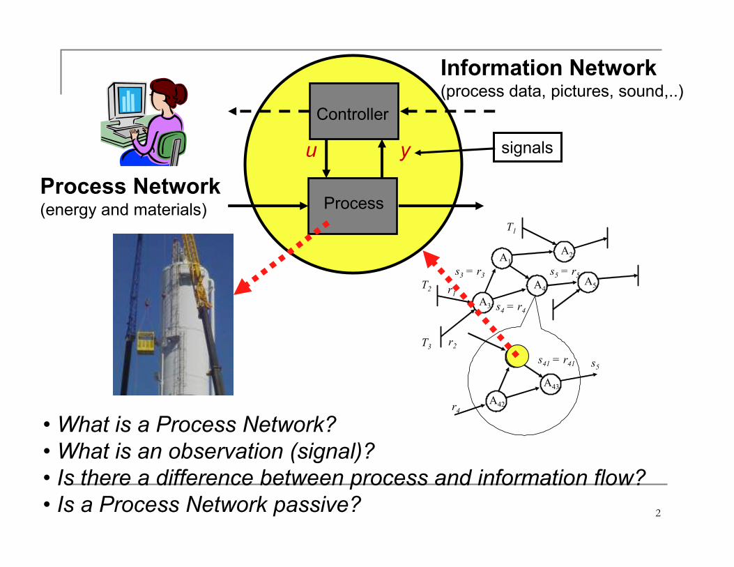
•What is a Process Network?
•What is an observation (signal)?
• Is there a difference between process and information flow?
• Is a Process Network passive?
Controller
Information Network(process data, pictures, sound,..)
Process Network (energy and materials)
A1
A2
A3
A4A5
A41
A42
A43
r1
r2
s3 = r3
s4 = r4
s5 = r5
s5s41 = r41
T3
T2
T1
r4
signals

3
Passivity Based Control
u yControl system:
nsobservatio )(
system control ),()(
xhy
uxgxfdt
dx
=
+=
S
χ
α
χ
VV
vχvm
rFv
rvr
ii
i
ii
iii
3
)(
=
−+=
+=
&
&
&
Example: MD with thermostat
strain
friction
4
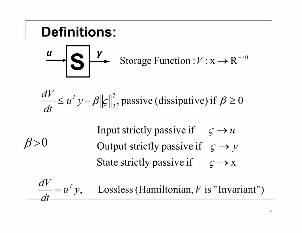
0 if ve)(dissipati passive ,2
2≥−≤ βςβyu
dt
dV T
x if passivestrictly State
if passivestrictly Output
if passivestrictly Input
→
→
→
ςςς
y
u
)Invariant"" is an,(Hamiltoni Lossless , Vyudt
dV T=
u y
S
Definitions:
0/Rx: :Function Storage +→V
0>β
5
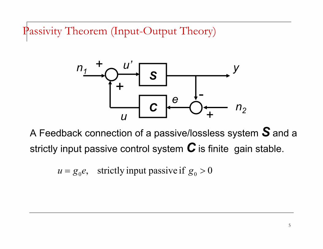
Passivity Theorem (Input-Output Theory)
S
eC
A Feedback connection of a passive/lossless system S and a
strictly input passive control system C is finite gain stable.
n1
+
+
-
+n2
u
y
0 if passiveinput strictly , 00 >= gegu
u’
6
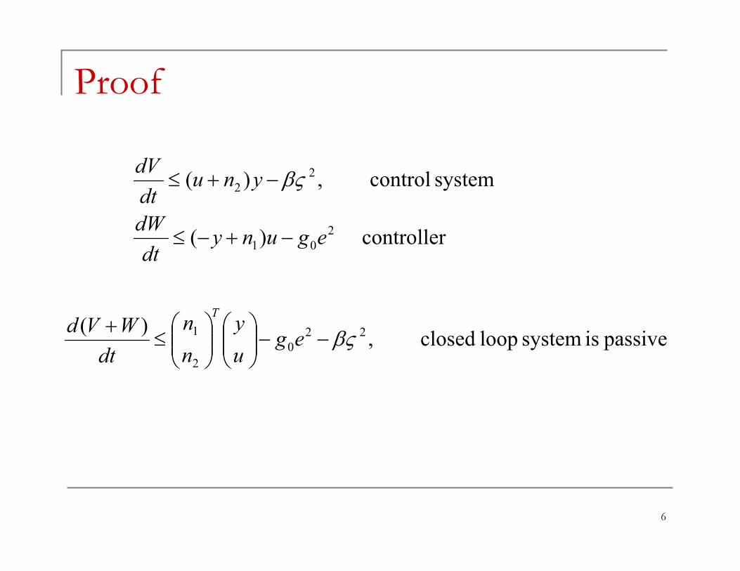
Proof
controller )(
system control ,)(
2
01
2
2
egunydt
dW
ynudt
dV
−+−≤
−+≤ βς
passive is system loop closed ,)( 22
0
2
1 βς−−
≤
+eg
u
y
n
n
dt
WVdT
7
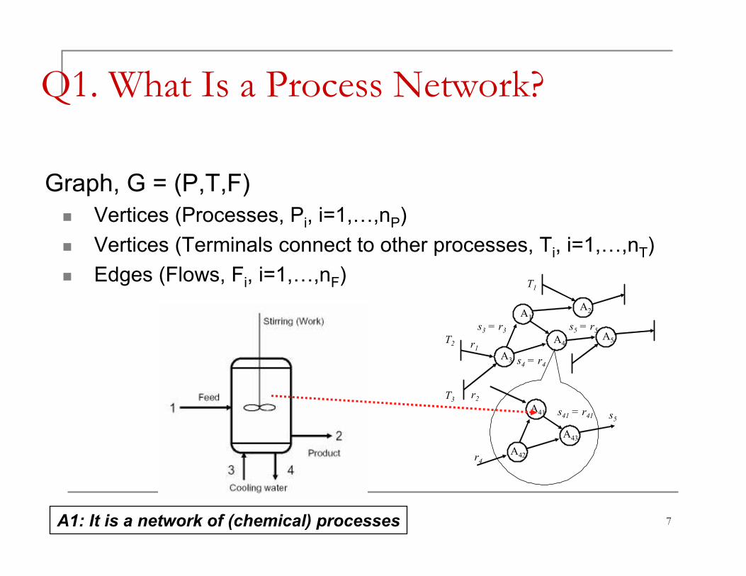
Q1. What Is a Process Network?
A1
A2
A3
A4A5
A41
A42
A43
r1
r2
s3 = r3
s4 = r4
s5 = r5
s5s41 = r41
T3
T2
T1
r4
Graph, G = (P,T,F)
� Vertices (Processes, Pi, i=1,…,nP)
� Vertices (Terminals connect to other processes, Ti, i=1,…,nT)
� Edges (Flows, Fi, i=1,…,nF)
A1: It is a network of (chemical) processes
8
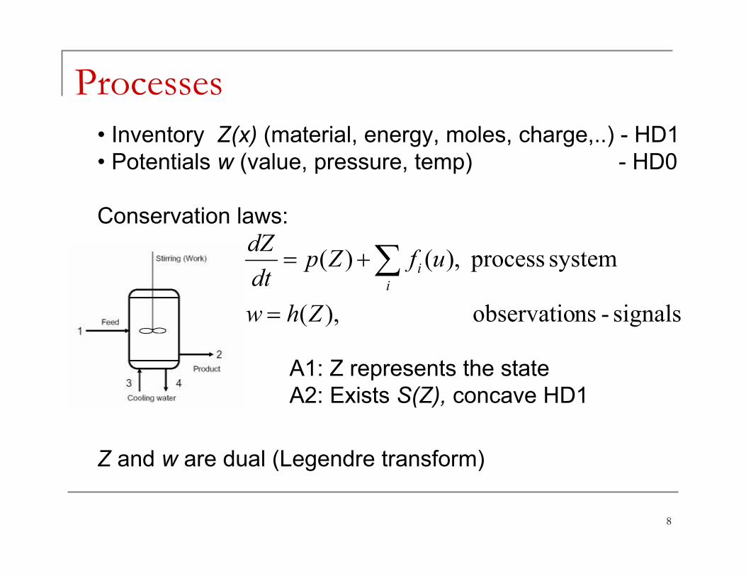
Processes
• Inventory Z(x) (material, energy, moles, charge,..) - HD1
• Potentials w (value, pressure, temp) - HD0
Conservation laws:
signals - nsobservatio ),(
system process ,)()(
Zhw
ufZpdt
dZ
i
i
=
+= ∑
A1: Z represents the state
A2: Exists S(Z), concave HD1
Z and w are dual (Legendre transform)
9
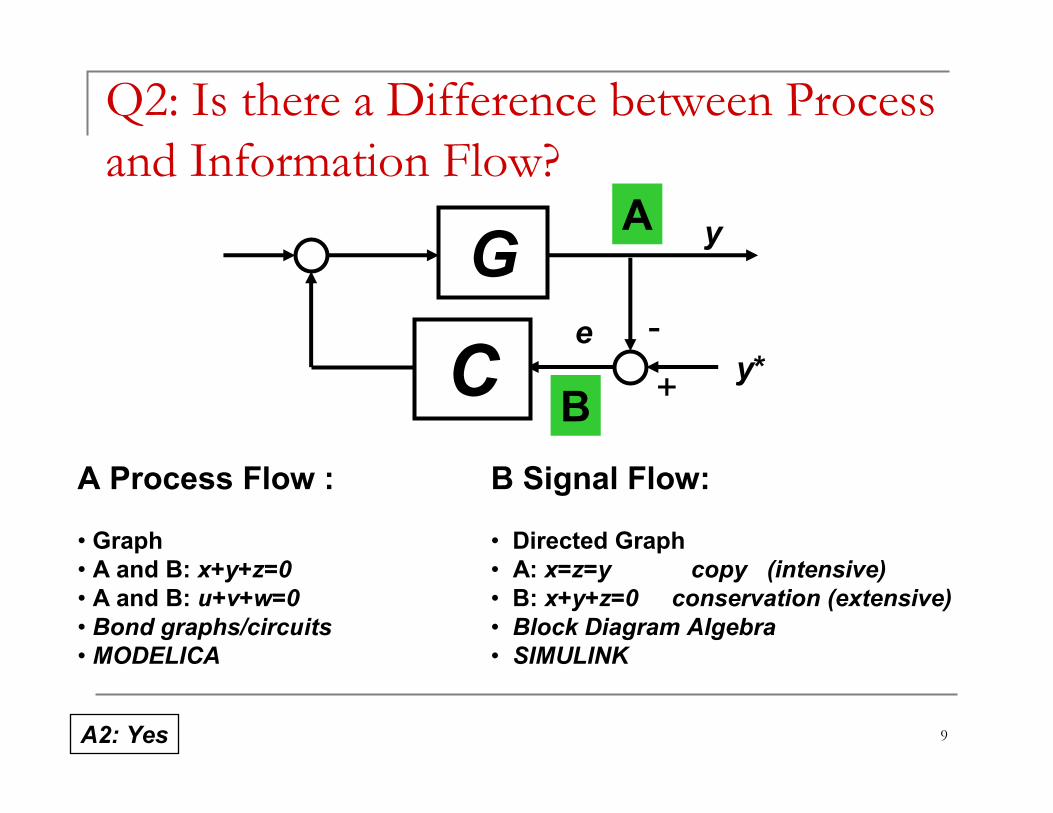
Q2: Is there a Difference between Process
and Information Flow?
B Signal Flow:
• Directed Graph
• A: x=z=y copy (intensive)
• B: x+y+z=0 conservation (extensive)
• Block Diagram Algebra
• SIMULINK
A Process Flow :
• Graph
• A and B: x+y+z=0
• A and B: u+v+w=0
• Bond graphs/circuits
• MODELICA
G A
BC
A2: Yes
e
y
y*
-
+
10
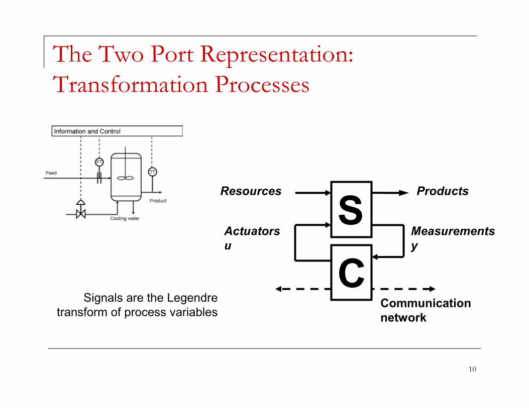
The Two Port Representation:
Transformation Processes
C
Resources Products
SActuators
u
Measurements
y
Communication
network
Signals are the Legendre
transform of process variables
11
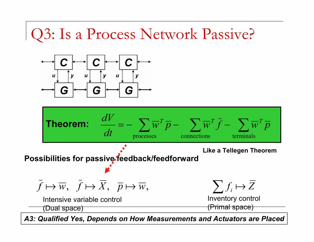
∑∑∑ −−−=terminalssconnectionprocesses
pwfwpwdt
dV TTT
∑ ZfwpXfwf i aaaa , , ,
Possibilities for passive feedback/feedforward
Theorem:
Like a Tellegen Theorem
Intensive variable control
(Dual space)
Inventory control
(Primal space)
Q3: Is a Process Network Passive?
A3: Qualified Yes, Depends on How Measurements and Actuators are Placed
12
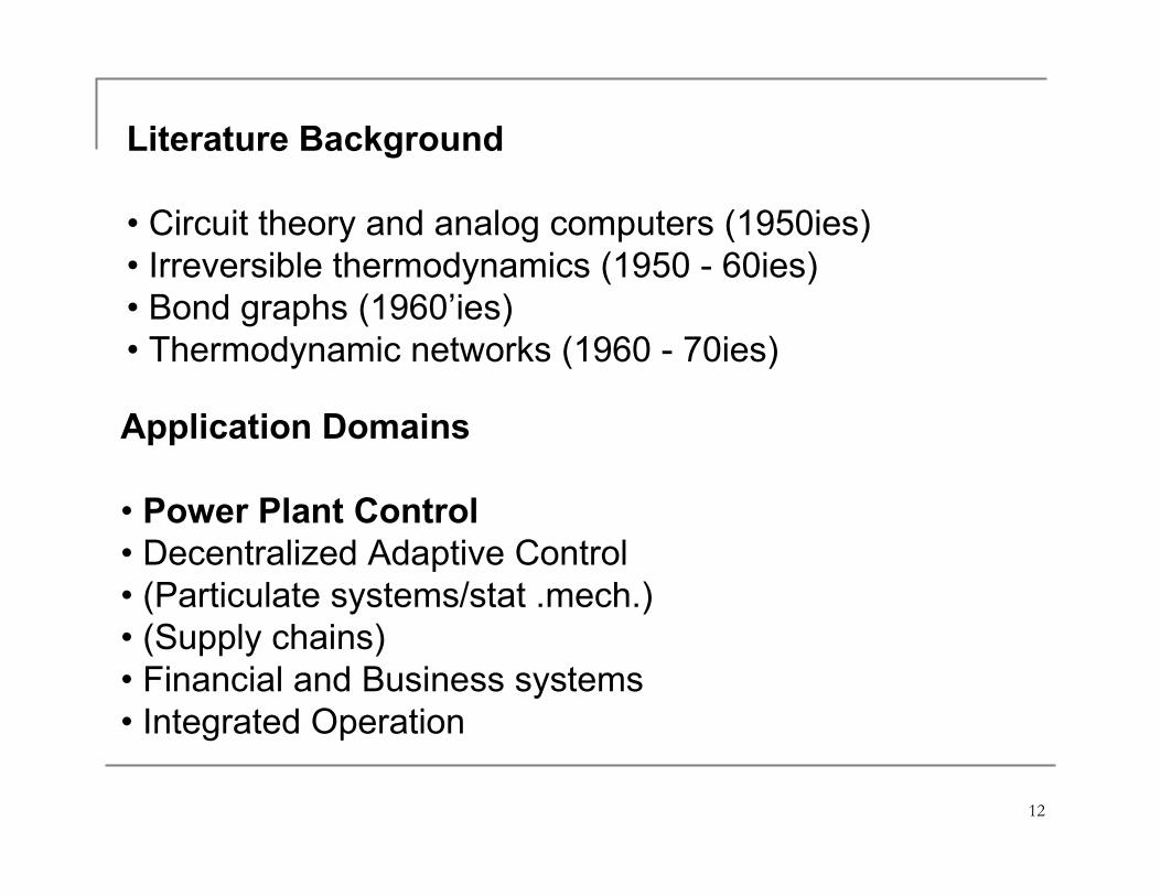
Literature Background
• Circuit theory and analog computers (1950ies)
• Irreversible thermodynamics (1950 - 60ies)
• Bond graphs (1960’ies)
• Thermodynamic networks (1960 - 70ies)
Application Domains
• Power Plant Control
• Decentralized Adaptive Control
• (Particulate systems/stat .mech.)
• (Supply chains)
• Financial and Business systems
• Integrated Operation
13
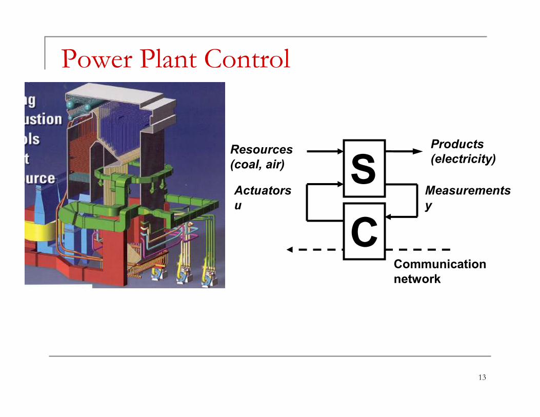
C
Resources
(coal, air)
Products
(electricity)
SActuators
u
Measurements
y
Communication
network
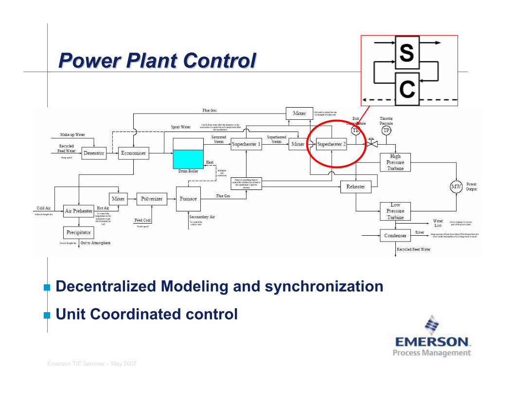
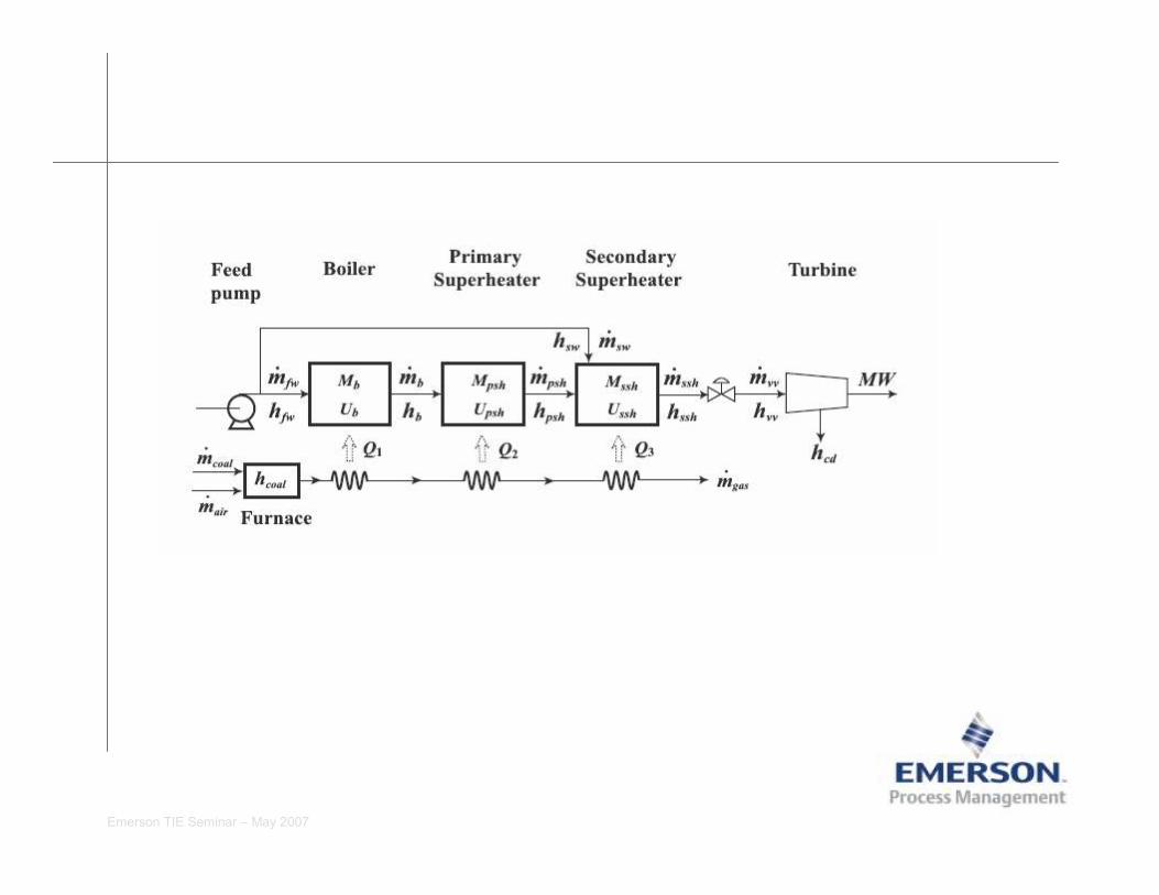
Power Plant ControlPower Plant Control
Emerson TIE Seminar – May 2007
Power Plant ControlPower Plant ControlPower Plant Control
� Decentralized Modeling and synchronization
� Unit Coordinated control

Emerson TIE Seminar – May 2007
Integrated Unit Master ApproachIntegrated Unit Master ApproachIntegrated Unit Master Approach
� Provides index for total control of unit
� Allows operator entered megawatt target and ramp rate
� Provides seven modes of unit operation
� Allows operator entered high and low limits
� Provides local and remote unit dispatch
� Built-in unit runbacks, rundowns and inhibits
Load Demand Dispatch
Emerson TIE Seminar – May 2007
Emerson TIE Seminar – May 2007
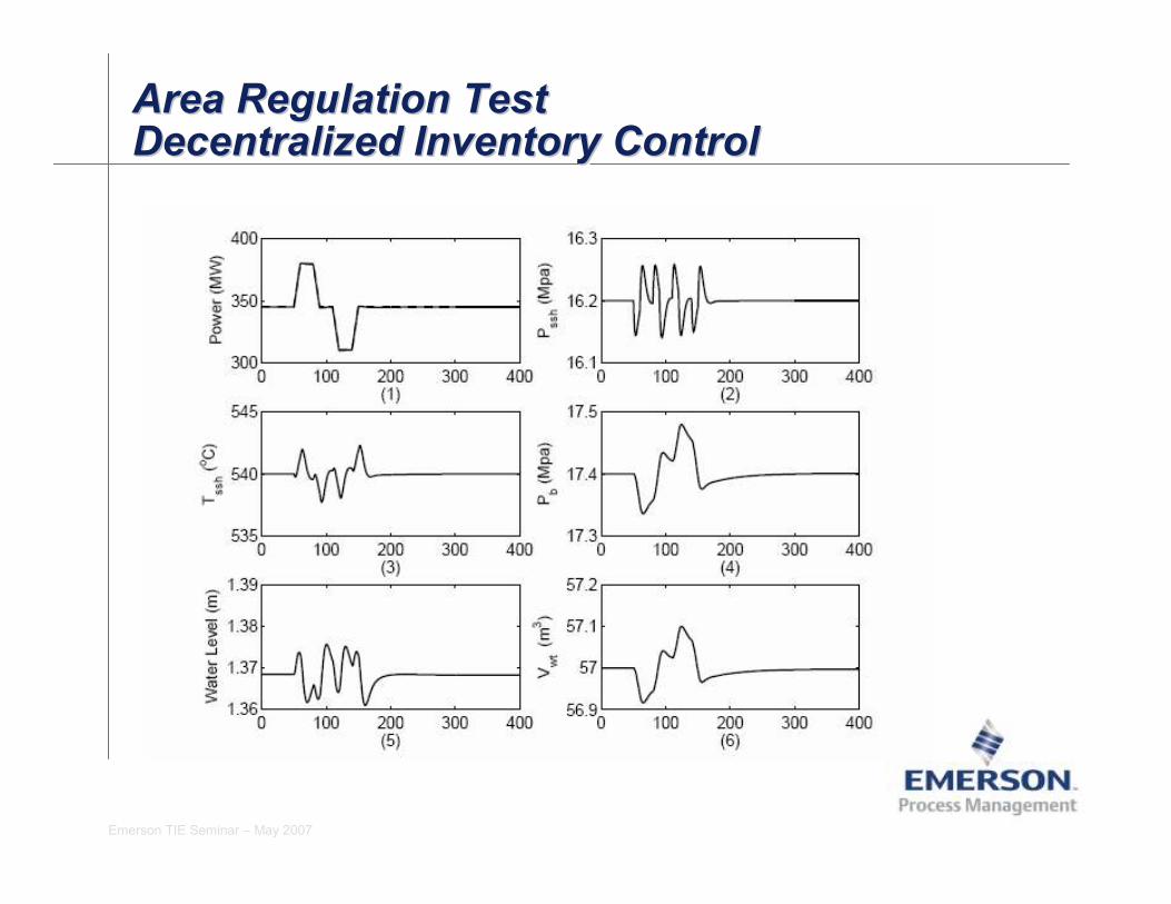
Area Regulation Test Decentralized Inventory ControlArea Regulation Test Area Regulation Test Decentralized Inventory ControlDecentralized Inventory Control
18
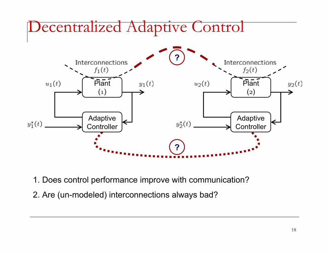
Decentralized Adaptive Control
Plant()
Plant()
?
1. Does control performance improve with communication?
?
2. Are (un-modeled) interconnections always bad?
Adaptive
Controller
Adaptive
Controller
19
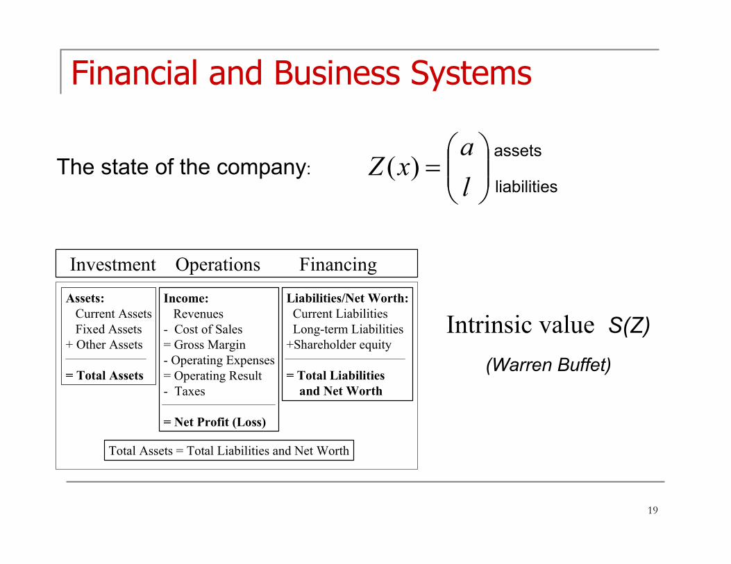
Financial and Business Systems
Intrinsic value S(Z)
(Warren Buffet)
=
l
axZ )(
assets
liabilities
Investment Operations Financing
Assets:
Current Assets
Fixed Assets
+ Other Assets
= Total Assets
Income:
Revenues
- Cost of Sales
= Gross Margin
- Operating Expenses
= Operating Result
- Taxes
= Net Profit (Loss)
Liabilities/Net Worth:
Current Liabilities
Long-term Liabilities
+Shareholder equity
= Total Liabilities
and Net Worth
Total Assets = Total Liabilities and Net Worth
The state of the company:
20
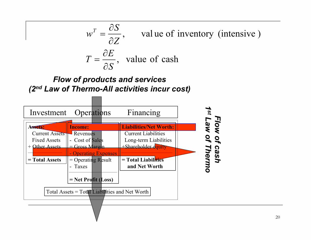
Investment Operations Financing
Assets:
Current Assets
Fixed Assets
+ Other Assets
= Total Assets
Income:
Revenues
- Cost of Sales
= Gross Margin
- Operating Expenses
= Operating Result
- Taxes
= Net Profit (Loss)
Liabilities/Net Worth:
Current Liabilities
Long-term Liabilities
+Shareholder equity
= Total Liabilities
and Net Worth
Total Assets = Total Liabilities and Net Worth
Flow of products and services
(2nd Law of Thermo-All activities incur cost)Flow of cash
1stLaw of T
herm
o
cash of value,
)(intensiveinventory of ue val,
S
ET
Z
SwT
∂∂
=
∂∂
=
21
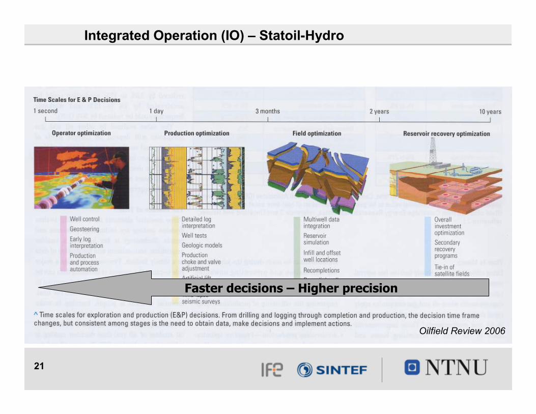
Oilfield Review 2006
Faster decisions – Higher precision
Integrated Operation (IO) – Statoil-Hydro

22
• Conservation Laws (KCL = 1st Law of Thermo)
• Dissipation (KVL = Second Law of Thermo)
Market
23
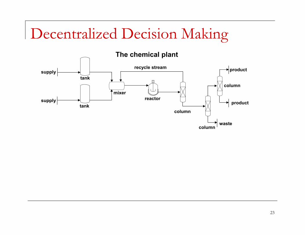
Decentralized Decision Making The chemical plant
tank
tank
mixer
reactor
column
column
column
product
product
waste
supply
supply
recycle stream
24
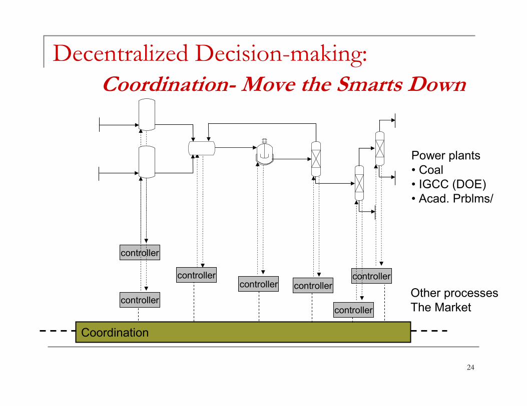
controller
controller
controllercontroller controller
controller
controller
Decentralized Decision-making:
Coordination- Move the Smarts Down
Coordination
Other processes
The Market
Power plants
• Coal
• IGCC (DOE)
• Acad. Prblms/
25
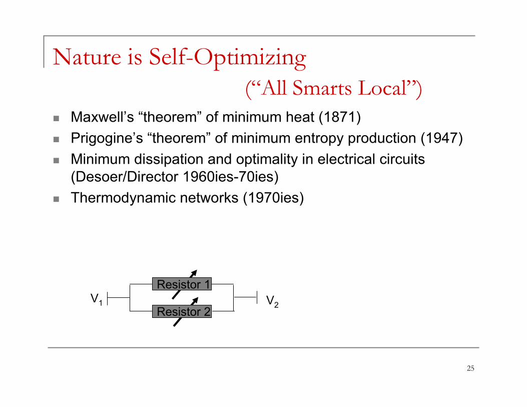
Nature is Self-Optimizing
(“All Smarts Local”)
� Maxwell’s “theorem” of minimum heat (1871)
� Prigogine’s “theorem” of minimum entropy production (1947)
� Minimum dissipation and optimality in electrical circuits
(Desoer/Director 1960ies-70ies)
� Thermodynamic networks (1970ies)
Resistor 1
Resistor 2 V1 V2
26
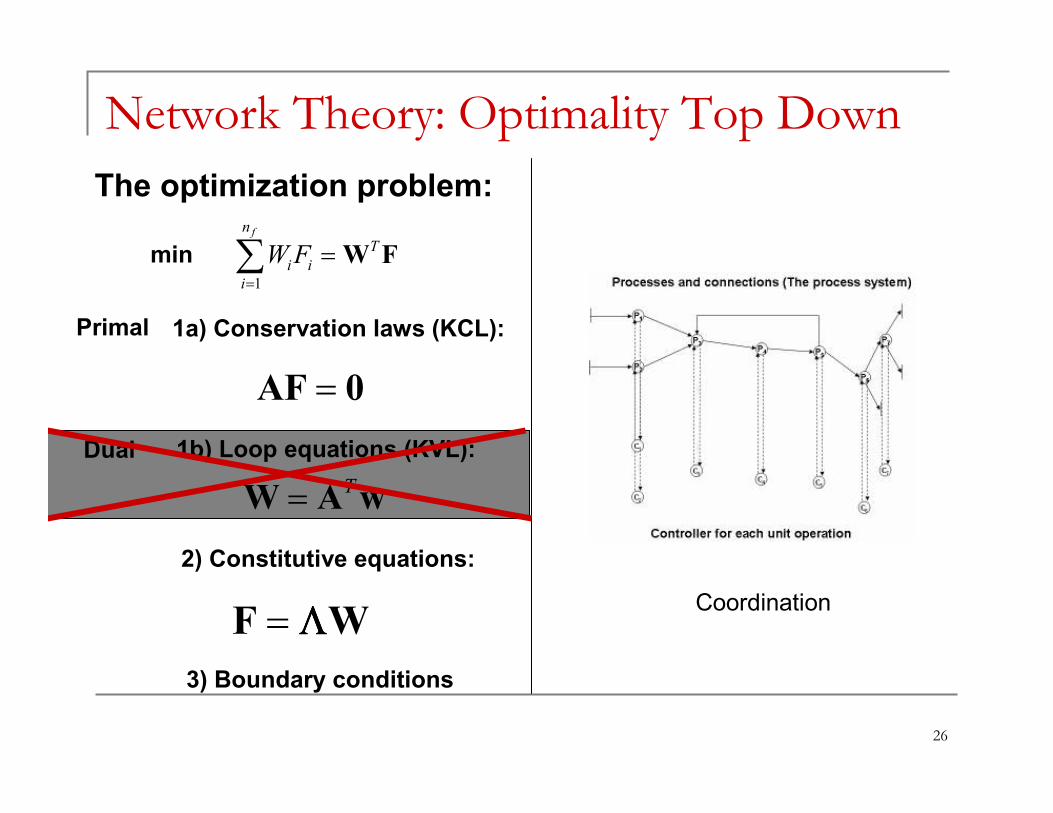
Network Theory: Optimality Top Down
=AF 0
T=W A w
1a) Conservation laws (KCL):
1b) Loop equations (KVL):
2) Constitutive equations:
=F WΛΛΛΛ3) Boundary conditions
The optimization problem:
1
fn
T
i i
i
W F=
=∑ W Fmin
Primal
Dual
Coordination
27
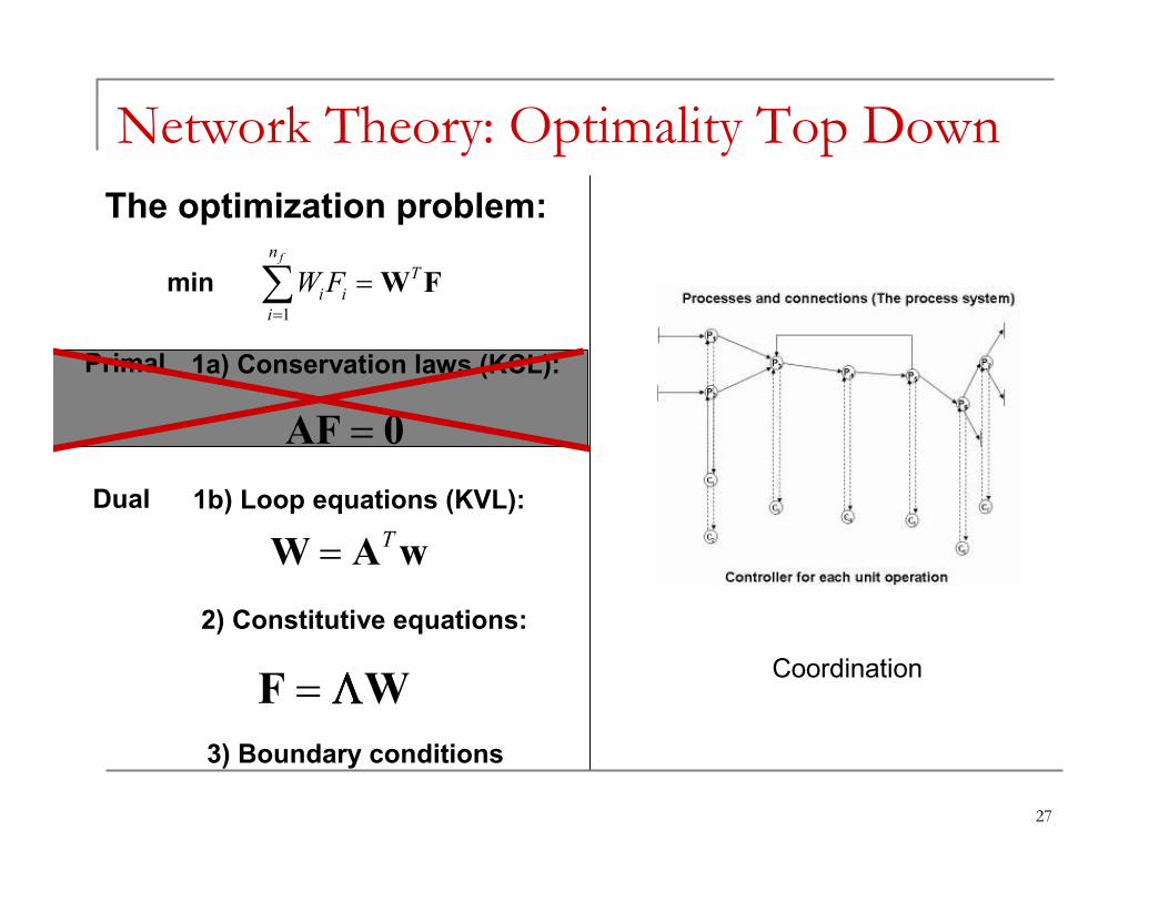
Network Theory: Optimality Top Down
=AF 0
T=W A w
1a) Conservation laws (KCL):
1b) Loop equations (KVL):
2) Constitutive equations:
=F WΛΛΛΛ3) Boundary conditions
The optimization problem:
1
fn
T
i i
i
W F=
=∑ W Fmin
Primal
Dual
Coordination
28
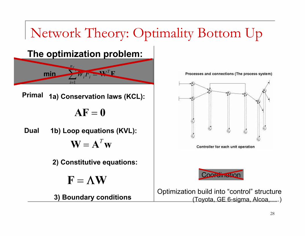
Network Theory: Optimality Bottom Up
=AF 0
T=W A w
1a) Conservation laws (KCL):
1b) Loop equations (KVL):
2) Constitutive equations:
=F WΛΛΛΛ3) Boundary conditions
The optimization problem:
1
fn
T
i i
i
W F=
=∑ W Fmin
Primal
Dual
Coordination
Optimization build into “control” structure(Toyota, GE 6-sigma, Alcoa,…..)
29
Conclusions
• Two port description proposed to represent the interface between
(process) systems and signals (the information system)
• Conservation laws and passivity theory can be applied for
stability analysis of process networks
• Stability and (Global) optimality follows from passivity theory if
flow is derived from a “convex potential”


