Next page Everything (Adequacy, Fairness, & Efficiency) Spending, Taxing, Saving, and Borrowing A balanced budget Portfolio management Hedging Self-insurance Optimal spending rules Fred Thompson Atkinson Graduate School of Management Willamette University
Transcript
Next page
A Theory of Everything (Adequacy, Fairness, & Efficiency)
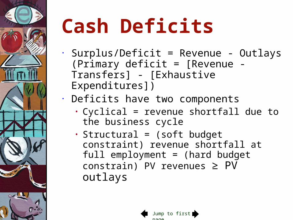
• Deficits have two components• Cyclical = revenue shortfall due to the
business cycle• Structural = (soft budget constraint) revenue
shortfall at full employment = (hard budget constrain) PV revenues ≥ PV outlays
Jump to first page
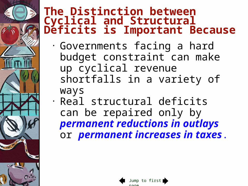
The Distinction between Cyclical and Structural Deficits is Important Because
• Governments facing a hard budget constraint can make up cyclical revenue shortfalls in a variety of ways
• Real structural deficits can be repaired only by permanent reductions in outlays or permanent increases in taxes.
Jump to first page
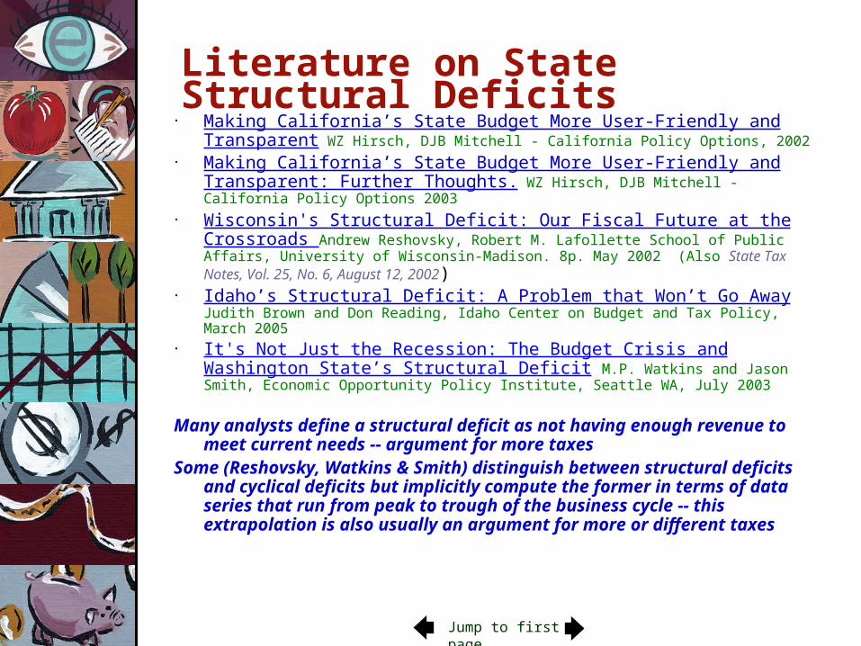
Literature on State Structural Deficits• Making California’s State Budget More User-Friendly and Transparent
WZ Hirsch, DJB Mitchell - California Policy Options, 2002• Making California’s State Budget More User-Friendly and Transparent:
Further Thoughts. WZ Hirsch, DJB Mitchell - California Policy Options 2003• Wisconsin's Structural Deficit: Our Fiscal Future at the Crossroads
Andrew Reshovsky, Robert M. Lafollette School of Public Affairs, University of Wisconsin-Madison. 8p. May 2002 (Also State Tax Notes, Vol. 25, No. 6, August 12, 2002)
• Idaho’s Structural Deficit: A Problem that Won’t Go Away Judith Brown and Don Reading, Idaho Center on Budget and Tax Policy, March 2005
• It's Not Just the Recession: The Budget Crisis and Washington State’s Structural Deficit M.P. Watkins and Jason Smith, Economic Opportunity Policy Institute, Seattle WA, July 2003
Many analysts define a structural deficit as not having enough revenue to meet current needs -- argument for more taxes
Some (Reshovsky, Watkins & Smith) distinguish between structural deficits and cyclical deficits but implicitly compute the former in terms of data series that run from peak to trough of the business cycle -- this extrapolation is also usually an argument for more or different taxes
Jump to first page
The Business Cycle
The phases of the business cycle are:• Expansion,• Peak (or boom),• Contraction, and,• Recessionary trough.
The duration of business cycles is irregular and the magnitude of the swings varies.
Jump to first page
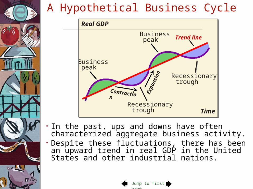
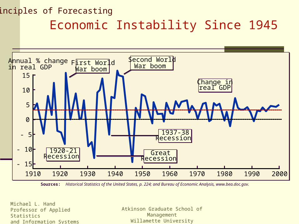
• In the past, ups and downs have often characterized aggregate business activity.
• Despite these fluctuations, there has been an upward trend in real GDP in the United States and other industrial nations.
Time
Real GDP
Business peak
Recessionary trough
Contraction Exp
ansi
on
A Hypothetical Business Cycle
Business peak
Recessionary trough
Trend line
Jump to first page
Source: Economic Report of the President, various issues.
The Business Cycle
6
8
4
2
0
- 2
1960 1965 1970 1975 1980 1985 1990 1995 2000
Annual growth rate of real GDP
Long-run growth rate(approx. 3%)
Jump to first page
.
- 15%- 10%- 5%
0% 5%10%15%20%
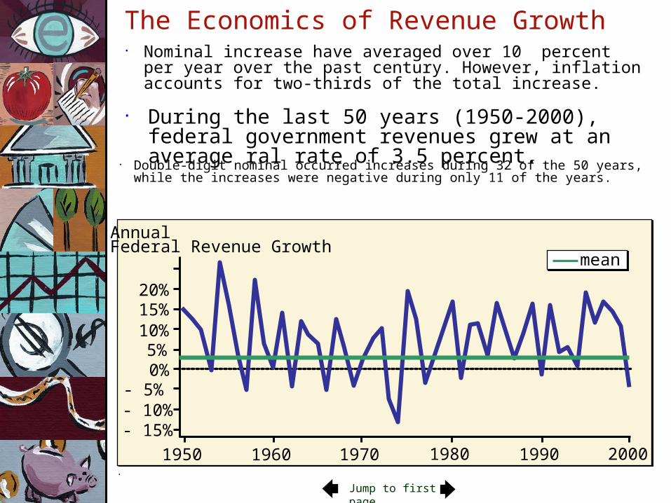
Annual Federal Revenue Growth
1950 1960 1970 1980 1990 2000
The Economics of Revenue Growth• Nominal increase have averaged over 10 percent per year
over the past century. However, inflation accounts for two-thirds of the total increase.
• During the last 50 years (1950-2000), federal government revenues grew at an average ral rate of 3.5 percent.
• Double-digit nominal occurred increases during 32 of the 50 years, while the increases were negative during only 11 of the years.
mean
Jump to first page
Sources: Derived from computerized data supplied by FAME ECONOMICS. Also see Economic Report of the President (annual).
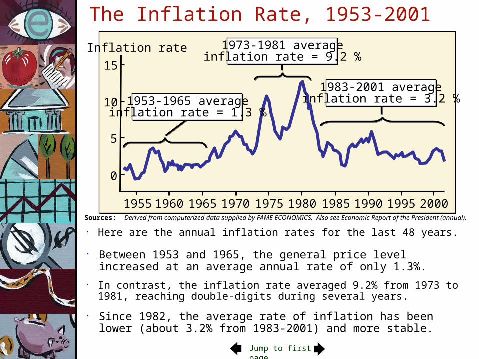
• Between 1953 and 1965, the general price level increased at an average annual rate of only 1.3%.
• Here are the annual inflation rates for the last 48 years.
• In contrast, the inflation rate averaged 9.2% from 1973 to 1981, reaching double-digits during several years.
• Since 1982, the average rate of inflation has been lower (about 3.2% from 1983-2001) and more stable.
The Inflation Rate, 1953-2001
1955 1960 1965 1970 1975 1980 1985 1990 20001995
10
5
0
Inflation rate
15
1953-1965 averageinflation rate = 1.3 %
1973-1981 averageinflation rate = 9.2 %
1983-2001 averageinflation rate = 3.2 %
Jump to first page
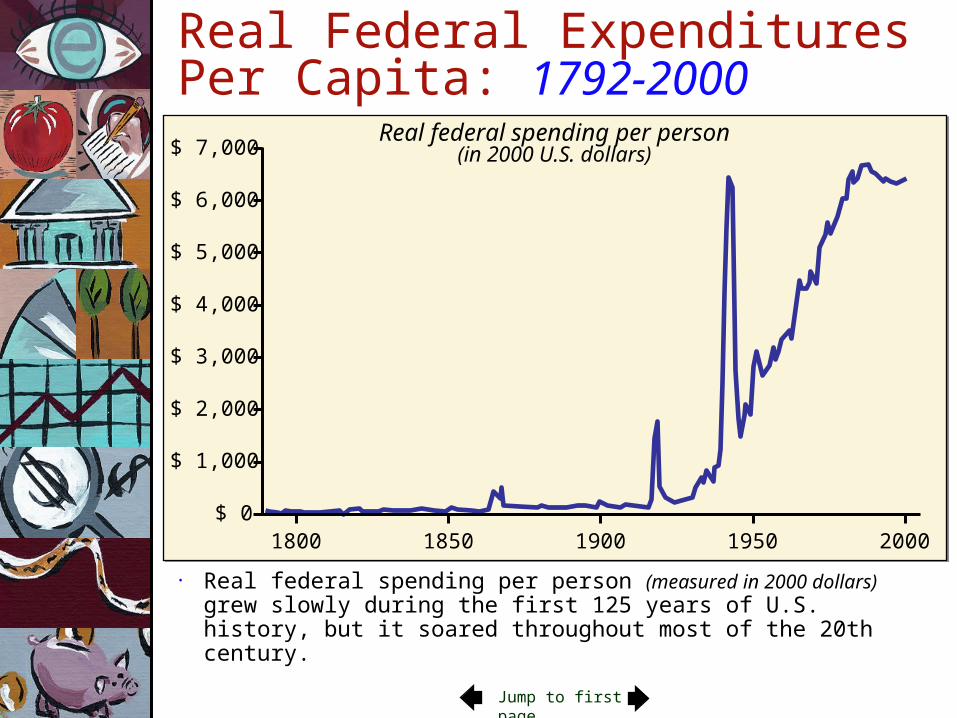
Real Federal Expenditures Per Capita: 1792-2000
• Real federal spending per person (measured in 2000 dollars) grew slowly during the first 125 years of U.S. history, but it soared throughout most of the 20th century.
$ 7,000
$ 6,000
$ 5,000
$ 4,000
$ 3,000
$ 2,000
$ 1,000
$ 01800 1850 1900 1950 2000
Real federal spending per person(in 2000 U.S. dollars)
Jump to first page
Federal Expenditures and Revenues
• The federal deficit or surplus as a share of the economy is shown here. Note the growth of budget deficits during the 1980s and the movement to surpluses during the 1990s.
18
20
22
24
1960 1965 1970 1975 1980 1985 1990 1995 2000
Expenditures
Revenues
Expenditures
Federal Government Expenditures and Revenues(as a share of GDP)
Source: Economic Report of the President, 2001. Note, recessions are indicated by shaded bars.
Jump to first page
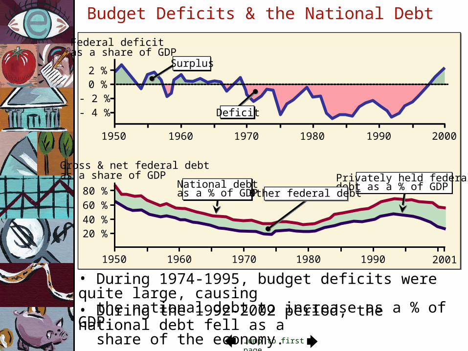
Budget Deficits & the National Debt
• Through most of the 1950s & 1960s, federal budget deficits were small as a % of GDP; occasionally there was a surplus.• During this period, the national debt declined as a % of GDP.
1950 1960 1970 1980 1990 2000
2 %
- 2 %- 4 %
0 %
Federal deficitas a share of GDP
1950 1960 1970 1980 1990 2001
80 %
40 %20 %
60 %
Privately held federaldebt as a % of GDPNational debt
as a % of GDP Other federal debt
Surplus
Deficit
Gross & net federal debtas a share of GDP
Jump to first page
Budget Deficits & the National Debt
1950 1960 1970 1980 1990 2000
2 %
- 2 %- 4 %
0 %
Federal deficitas a share of GDP
1950 1960 1970 1980 1990 2001
80 %
40 %20 %
60 %
Privately held federaldebt as a % of GDPNational debt
as a % of GDP Other federal debt
Surplus
Deficit
Gross & net federal debtas a share of GDP
• During 1974-1995, budget deficits were quite large, causing the national debt to increase as a % of GDP.• During the 1992-2002 period, the national debt fell as a share of the economy.
Jump to first page
This is what Happened after2001
Jump to first page
Conclusions• More than half of the federal government’s
deficits over the past fifty years were cyclical in nature.
• Between 1976-1993, structural deficits were between 1 and 3 percent of GDP.
• After 1994, the federal deficit was eliminated by a combination of spending restraint, revenue increases, and boom.
• After 2001 spending increased, taxes were cut, and we had a slight recession, reestablishing a structural deficit of 1 to 3 percent of GDP.
• Then came the Great Recession!
Jump to first page
State Deficits• Most states have less volatile revenue structures than
the federal government• Even so they often experience substantial cyclical
fiscal effects• Because most are required to balance their budgets,
structural deficits mean something different for states: Surpluses must equal deficits over the course of the business cycle
• Rainy day funds (savings)• Countercyclical borrowing• Hedging
See C. Hinkelmann & Steve Swidler, “Macroeconomic Hedging with Existing Futures Contracts,” Risk Letters, forthcoming; “State Government Hedging with Financial Derivatives,” State and Local Government Review, volume 37:2, 2005; “Using Futures Contracts to Hedge Macroeconomic Risks in the Public Sector,” Trading and Regulation, volume 10, number 1, 2004.
See C. Hinkelmann & Steve Swidler, “Macroeconomic Hedging with Existing Futures Contracts,” Risk Letters, forthcoming; “State Government Hedging with Financial Derivatives,” State and Local Government Review, volume 37:2, 2005; “Using Futures Contracts to Hedge Macroeconomic Risks in the Public Sector,” Trading and Regulation, volume 10, number 1, 2004.
Jump to first page
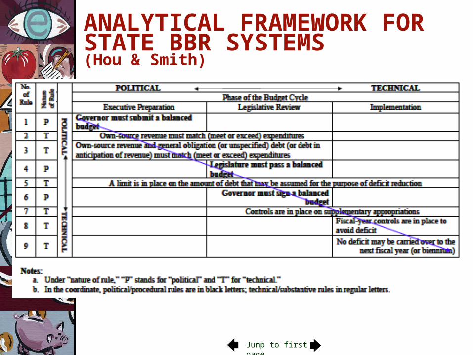
ANALYTICAL FRAMEWORK FOR STATE BBR SYSTEMS (Hou & Smith)
Jump to first page
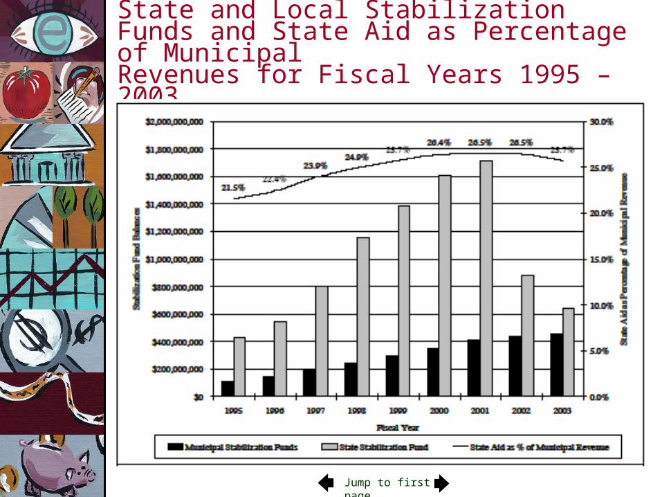
State and Local Stabilization Funds and State Aid as Percentage of MunicipalRevenues for Fiscal Years 1995 – 2003
Jump to first page
Oregon’s Fiscal GapPrimarily (but not entirely) Driven by Revenues (actual revenues - CSB)
Budget Shortfall/Surplus over Time
-400
-300
-200
-100
0
100
200
300
1980 1985 1990 1995 2000 2005
Year
Magnitude of Shortfall/Suprlus (in Millions, Real 2002$)
Jump to first page
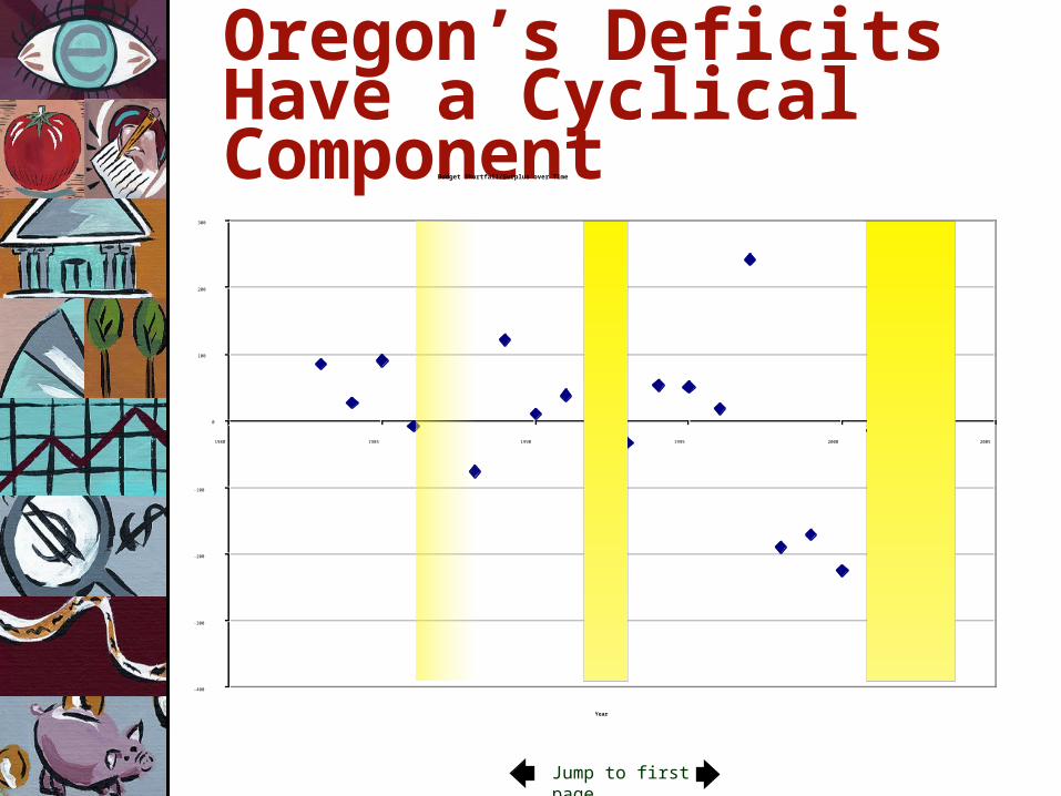
Oregon’s Deficits Have a Cyclical Component
Budget Shortfall/Surplus over Time
-400
-300
-200
-100
0
100
200
300
1980 1985 1990 1995 2000 2005
Year
Magnitude of Shortfall/Suprlus (in Millions, Real 2002$)
Jump to first page
Analytical Problems
• We used negative job growth as a recession identifier because we lacked a formal mechanism to date recessions at the state level.
• That’s not entirely satisfactory.
Jump to first page
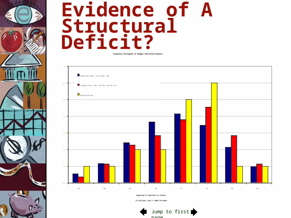
Evidence of A Structural Deficit?
Frequency Histogram of Budget Shortfall/Surplus
0
1
2
3
4
5
6
7
-137 -238 -163 -88 -13 63 138 213
Magnitude of Shortfall or Surplus
(in Millions, Real $ [2002 CPI=100])
Frequency
Normal Distn: Mean = -20, Std Dev = 140
Triangular Distn: Min = -350; Max = 250; ML = 69
Observed Cum Freq
Jump to first page
Problem• Doesn’t adjust for scale, just
inflation• Positive correlation between
budget gap and time could be due to structural deficit or to selection bias
Jump to first page
Analytical Solution
• Monte Carlo Simulation• Weiner Process• Trough to Trough Revenue
and Spending• Trough to Trough Spending,
Peak to Peak Revenues
Jump to first page
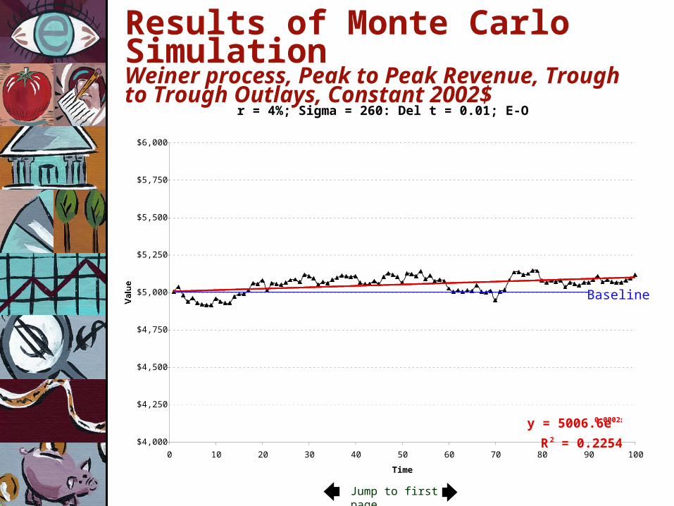
Results of Monte Carlo Simulation Weiner process, Peak to Peak Revenue, Trough to Trough Outlays, Constant 2002$
r = 4%; Sigma = 260: Del t = 0.01; E-O-Y = $5,116
y = 5006.6e0.0002x
R2 = 0.2254$4,000
$4,250
$4,500
$4,750
$5,000
$5,250
$5,500
$5,750
$6,000
0 10 20 30 40 50 60 70 80 90 100
Time
ValueBaseline
Jump to first page
Implications• Other things equal, revenue growth is
faster than outlay growth• Oregon doesn’t need to increase taxes to
offset a structural budget deficit• Oregon could rely on a rainy day fund of
sufficient size to mitigate the adverse consequences of cyclical revenue shortfalls (if it had one) or mitigate them via a program of countercyclical borrowing
• Hedging
Jump to first page
BUDGETING IN CHILE• Hierarchical budget institutions• The executive branch is solely
responsible for public financial management
• Concentration of responsibilities within the Executive and in the Ministry of Finance
Jump to first page
BUDGETING IN CHILE• Reflected in:
• Initiative to initiate legislation on budget and financial matters restricted to President
• Limited powers of the legislature to modify the budget
• Strict deadlines for budget approval by Congress
• Earmarking of taxes, loans from Central Bank forbidden by the Constitution
GI - Gross Income from the source indicated PItotal – Total Oregon Personal Income PIwages – Wage and Salary Component of Personal Income PIother_lab – Other labor component of Personal Income PIdir – Dividends, Interest and Rent component of Personal Income PIproprietors – Proprietors’ Income component of Personal Income MKTw5000 – Wilshire 5000 stock indexEMPretail – Oregon Retail Employment CORP_PROFIT – U.S. Corporate Profits POP_OR65+ – Oregon 65 and older population IR3mo_tbill – Discount rate of 3 month Treasury Bill FDIST1mil - Filer Distribution Model, Ratio of $1 million-plus filers to Total filers DMYtax_rate – Dummy variable for 1982 through 1984 tax rate increase
Personal Income Tax ModelOffice of Economic AnalysisDepartment of Administrative Services
Michael L. HandProfessor of Applied Statisticsand Information Systems
Atkinson Graduate School of ManagementWillamette University
Principles of Forecasting
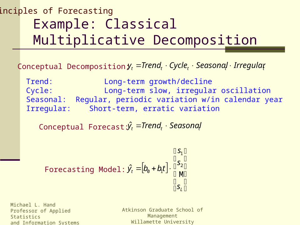
Projective Methods
Simple extrapolation in time Predictors are time and functions of time
Trend, seasonal, cyclical factors Minimal data/supporting forecast requirement Assumes current conditions will persist Best for short-term forecasts
One year out (two if we stretch) or less
Michael L. HandProfessor of Applied Statisticsand Information Systems
Atkinson Graduate School of ManagementWillamette University
Principles of Forecasting
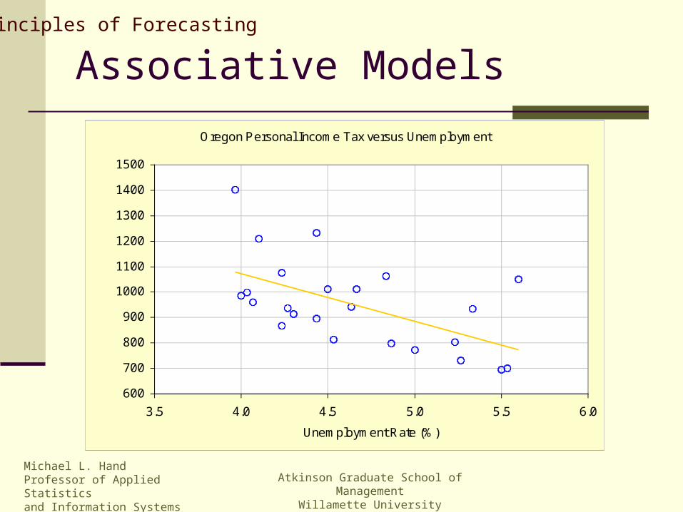
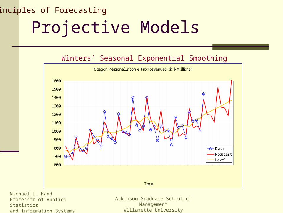
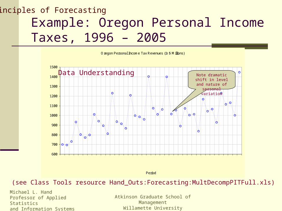
Projective Models
Oregon Personal Income Tax Revenues (in $ Millions)
Michael L. HandProfessor of Applied Statisticsand Information Systems
Atkinson Graduate School of ManagementWillamette University
Principles of Forecasting
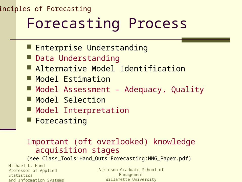
Forecasting Process
Enterprise Understanding Data Understanding Alternative Model Identification Model Estimation Model Assessment – Adequacy, Quality Model Selection Model Interpretation Forecasting
Important (oft overlooked) knowledge acquisition stages(see Class_Tools:Hand_Outs:Forecasting:NNG_Paper.pdf)
Michael L. HandProfessor of Applied Statisticsand Information Systems
Atkinson Graduate School of ManagementWillamette University
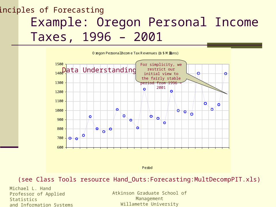
Principles of Forecasting
Oregon Personal Income Tax Revenues (in $ Millions)
Michael L. HandProfessor of Applied Statisticsand Information Systems
Atkinson Graduate School of ManagementWillamette University
Principles of Forecasting
Forecast Model Assessment
Residual analysis: A somewhat scatological endeavor, whereby we assess forecast quality through an analysis of residuals or what the forecast process leaves unexplained.
Residual (Error) = Actual – Forecast
Assessment possible for any type of forecasting process – statistical, organizational, ad hoc, arbitrary.
Michael L. HandProfessor of Applied Statisticsand Information Systems
Atkinson Graduate School of ManagementWillamette University
predict revenue growth from one year to the next or the timing of the business cycle, but we can make actuarial predictions
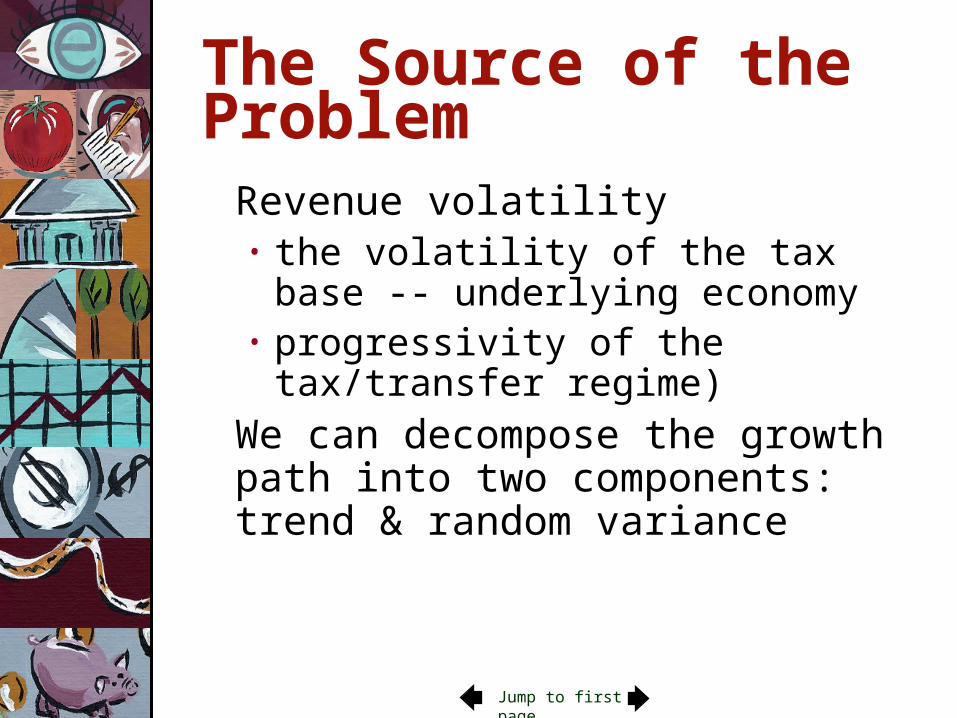
• Mean/variance analysis: trend + variance (systematic volatility and unsystematic volatility or noise)
Jump to first page
Forecast Model Assessment
Residual analysis:Residual = Actual – Trend
Residual = ErrorTrend = Forecast, mean rate of
growthResiduals can be described in terms
of Var or SD from mean rate of growth Var = volatility
Next page
Portfolio Theory
Jump to first page
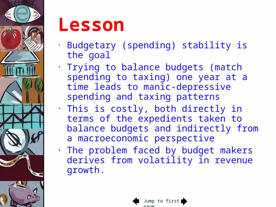
Lesson • Most states cannot significantly
reduce volatility in revenue growth by substituting one tax type for another (e.g. a broad-based goods and services taxes for an income tax, or vice versa).
Jump to first page
Lesson• Unsystematic volatility in revenue growth
can in theory be reduced via a well-designed portfolio of tax/transfer types.• Diversification can reduce revenue
volatility: most states rely on a portfolio of tax types.
• How does diversification of tax portfolios work? The answer is that portfolio volatility is a function of the covariance or correlation, , of its component revenue sources
Jump to first page
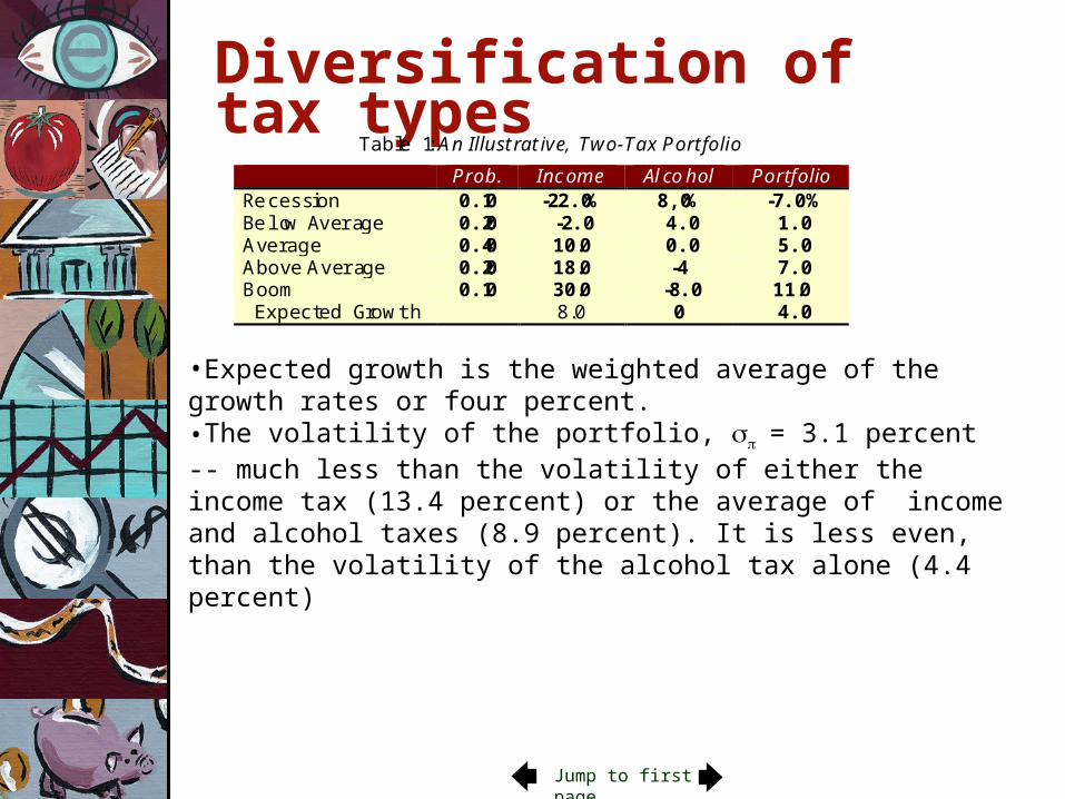
Diversification of tax typesTable 1: An Illustrative, Two-Tax Portfolio
Prob. Income Alcohol PortfolioRecession 0.10 -22.0% 8,0% -7.0%Below A vera ge 0.20 -2.0 4.0 1.0Aver age 0.40 10.0 0.0 5.0Above Avera ge 0.20 18.0 -4 7.0Boom 0.10 30.0 -8.0 11.0
Expect ed Gr owth 8.0 0 4.0
•Expected growth is the weighted average of the growth rates or four percent.•The volatility of the portfolio, = 3.1 percent -- much less than the volatility of either the income tax (13.4 percent) or the average of income and alcohol taxes (8.9 percent). It is less even, than the volatility of the alcohol tax alone (4.4 percent)
Jump to first page
Implications of portfolio theory
• In general, tax sources have 0.65, so adding taxes to the portfolio tends to reduce but not eliminate volatility.
• It is possible to construct an efficient growth frontier, showing an efficient linear combination of growth rates and volatilities ranging from zero volatility, to a state’s optimal volatility at its current growth rate and beyond
• All one needs is information on the covariance of the growth rates of each of the different tax types and designs that obtain in different states.
• Only if we look at efficient tax portfolios is there a necessary tradeoff between stability and growth
Jump to first page
Expected
Portfolio
Growth
Figure 6: Feasible and Efficient Tax Portfolios
Volatility,
PEFPE
Efficiency frontier
Theoretically feasible
OR
CS
SE
CY
PY
PE = Efficient Portfolio
PEF = Efficient and Fair Portfolio
OR = Current tax portfolio
CY = Corporate income tax
PY = Personal income tax
CS = Broad-based consumption tax
SE = Selected excises
Efficient Tax Portfolios
Jump to first page
Lesson• Average volatility will usually be reduced by
adding tax sources, except where the two taxes are perfectly correlated, r = +1.0
• A two tax portfolio could in theory be combined to eliminate revenue volatility completely, but only if r = -1.0 and the two taxes were weighted equally
• The portion of the volatility that cannot be eliminated via a portfolio of revenue and transfer types is known as systemic volatility; the portion that can, in theory, be eliminated is known as unsystematic volatility or noise
Jump to first page
Lesson• Once an efficient tax-portfolio
frontier has been identified, changes in the portfolio of tax types and transfers to increase tax-equity will also increase volatility in revenue growth
Jump to first page
Lesson• Even the best-designed tax portfolio
would not eliminate all volatility. In the absence of a policy of borrowing and lending at the risk free rate, the best tax-portfolio designers could do is eliminate the unsystematic or random portion of the variation in revenue growth.
• The systematic portion would remain. By systematic we mean, the portion correlated with some underlying variable
Jump to first page
Lesson• GNP growth is the main underlying
variable -- which has two components• Trend (mean)• Cyclical
• Predicting the timing and amplitude of business cycles is no easier than predicting the growth of the economy from one year to the next
Next page
Hedging and self insuranceOne way to eliminate systematic volatility in revenue growth is with a revenue flow of equal and opposite volatility. This is called hedging.
If we could find two tax types which produced revenue flows of the same size that were perfectly, but inversely correlated with each other, we could eliminate all volatility in revenue growth. Unfortunately, there are no such tax types.
Is it possible to design a hedge against the systematic component of revenue volatility?
Jump to first page
Lesson • It is theoretically possible to do so
using forwards, futures, or options
Jump to first page
Lesson • It is theoretically possible to do so
using forwards, futures, or options • It is not practically feasible to do
so at this time
Jump to first page
Lesson• It may never be politically
feasible to do so
Jump to first page
Hedging with options & futures contracts
See C. Hinkelmann & Steve Swidler, “Macroeconomic Hedging with Existing Futures Contracts,” Risk Letters, forthcoming; “State Government Hedging with Financial Derivatives,” State and Local Government Review, volume 37:2, 2005; “Using Futures Contracts to Hedge Macroeconomic Risks in the Public Sector,” Trading and Regulation, volume 10, number 1, 2004.
See C. Hinkelmann & Steve Swidler, “Macroeconomic Hedging with Existing Futures Contracts,” Risk Letters, forthcoming; “State Government Hedging with Financial Derivatives,” State and Local Government Review, volume 37:2, 2005; “Using Futures Contracts to Hedge Macroeconomic Risks in the Public Sector,” Trading and Regulation, volume 10, number 1, 2004.
• Futures• Options
Jump to first page
Self insurance?
• Rainy day fund• Cooperative cash pool
Jump to first page
LessonSelf insurance and risk pooling• Insurance is like a put option. • A rainy-day fund is simply a form of self
insurance.• A rainy day fund large enough to prevent
all revenue shortfalls would be very costly
• Risk pooling would dramatically reduce those costs
Next page
Optimal Spending
Jump to first page
Lesson• States can use savings and/or borrowing to smooth out
consumption over the business cycle• Consumption smoothing implies present value balance:
• Goal should be to balance budgets in a present-value sense, using savings and debt to smooth spending
• Hence, the problem faced by budgeters is to identify the maximum rate of growth in the spending level from one year to the next that is consistent with present value balance, given the state’s existing revenue/transfer structure and volatility.
• where PV future revenues + net assets < PV future exhaustive expenditures, permanent reductions in spending or permanent increases in taxes are necessary
Jump to first page
Lesson• This can be done by treating revenue
growth as a random walk. In which case, the problem faced by budget makers can be solved mathematically by optimal control theory or estimated via Monte Carlo simulation.
Jump to first page
The basic questionHow much should we spend next
year?State and local governments have few
degrees of freedom but can focus on issues of solvency and liquidity
Jump to first page
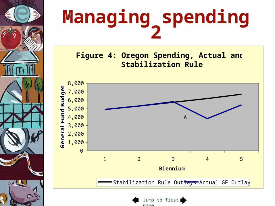
Managing spending• Schunk and Woodward’s (S&W)
spending rule: Increase spending no faster than the rate
of inflation plus the long-term real growth rate of the underlying economy
(put aside the remainder for a rainy day)
Donald Schunk and Douglas P. Woodward. Spending Stabilization Rules: A Solution to
Recurring State Budget Crises? 2005. Public Budgeting & Finance 5(4): 105-124.
Jump to first page
Managing spending 2
Figure 4: Oregon Spending, Actual and Stabilization Rule
0
1,000
2,000
3,000
4,000
5,000
6,000
7,000
8,000
1 2 3 4 5
Biennium
General Fund Budget
Stabilization Rule Outlays Actual GF Outlays
A
Jump to first page
Revenue growth is a random walkRevenue growth can be modeled as a Wiener process: • a continuous-time, continuous-state stochastic
process in which the distribution of future values conditional on current and past values is identical to the distribution of future values conditional on the current value alone, and
• the variance of the change in the process grows linearly with the time horizon.
Jump to first page
Monte Carlo simulation of Oregon’s future spending and revenues, given the adoption
of S&W’s spending rule
y = 2.6215xR2 = 0.5876
-$200
$0
$200
$400
$600
$800
$1,000
0 10 20 30 40 50 60 70 80 90 100
Time
Value
Jump to first page
A better spending ruleGiven that we can model revenue growth as a Wiener process, it is possible to calculate a spending rule directly using optimal control theory. By comparing proposed spending levels (including tax expenditures and debt service) against the optimum spending level calculated using this rule, one can say whether or not the specified spending level is sustainable and implicitly assess a state’s saving and borrowing policies as well.
Jump to first page
Findings
• Budgetary Growth = to geometric mean of revenue growth is closer to optimum than Budgetary Growth equal to arithmetic mean of nominal growth of the underlying economy
Jump to first page
Practical Implications• Oregon cannot significantly reduce volatility in
revenue growth by tinkering with its tax structure -- at least not without also reducing progressivity
• Hedging -- probably not practical• Oregon could rely on a rainy day fund of sufficient size
to mitigate the adverse consequences of cyclical revenue shortfalls (if it had one) or meliorate them via a program of countercyclical borrowing
• Other things equal, Oregon’s revenue growth trend is faster than outlay growth under the S&W rule
• Oregon doesn’t need to increase taxes to offset a structural budget deficit -- it could adopt an optimal spending rule that would allow it to smooth consumption
Next page
RANKING THE RANKING THE STATESSTATES
Jump to first page
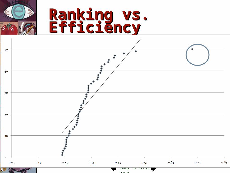
Ranking State & Ranking State & Local Tax SystemsLocal Tax Systems• Finding a way to rank
fairness, adequacy, and efficiency is difficult
• There are a lot of outliers
Jump to first page
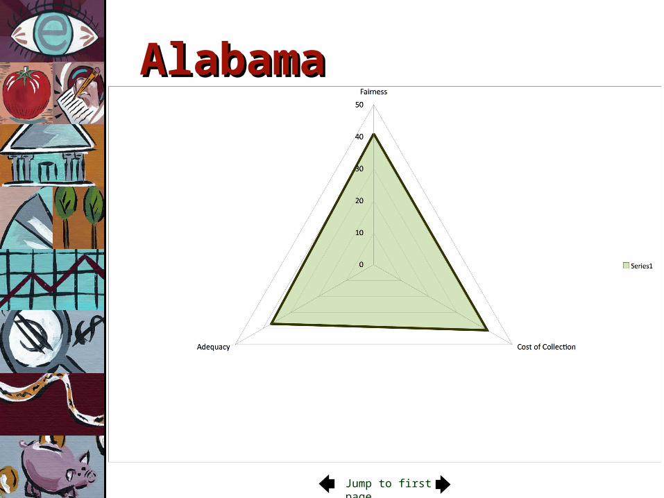
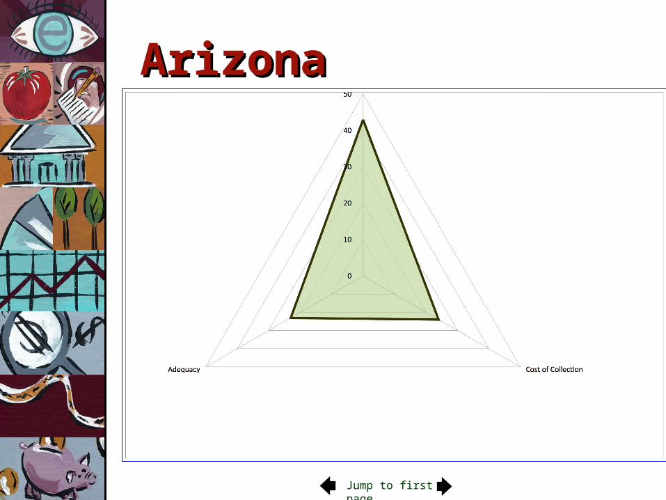
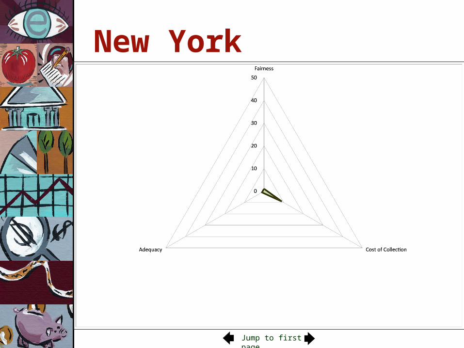
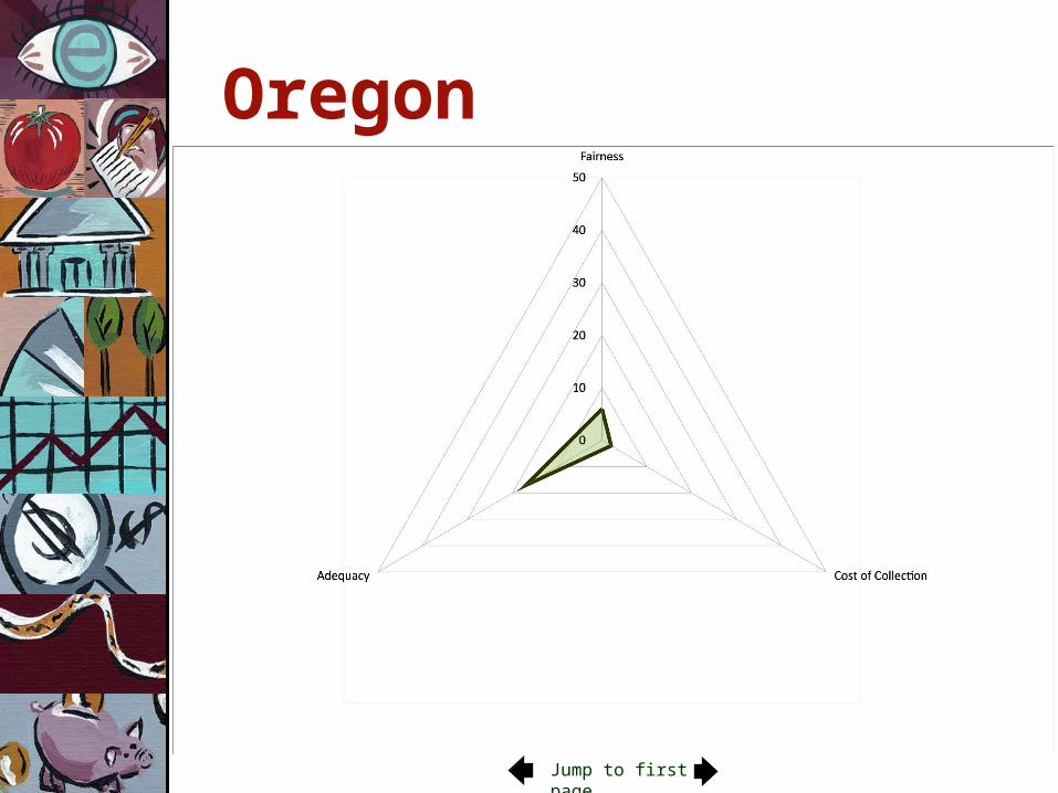
How does my state compare?
FairnessFairness
Jump to first page
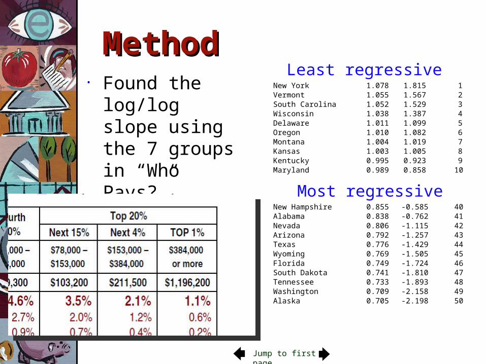
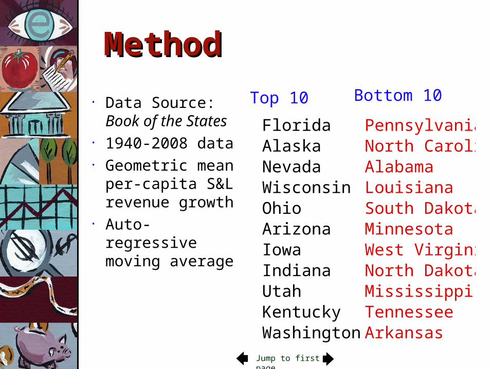
MethodMethod• Found the log/log
slope using the 7 groups in “Who Pays?”• Weighted OLS