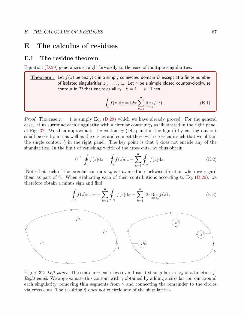
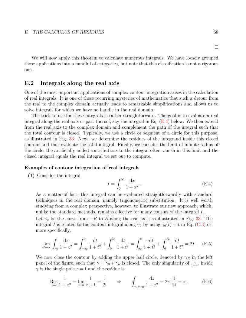
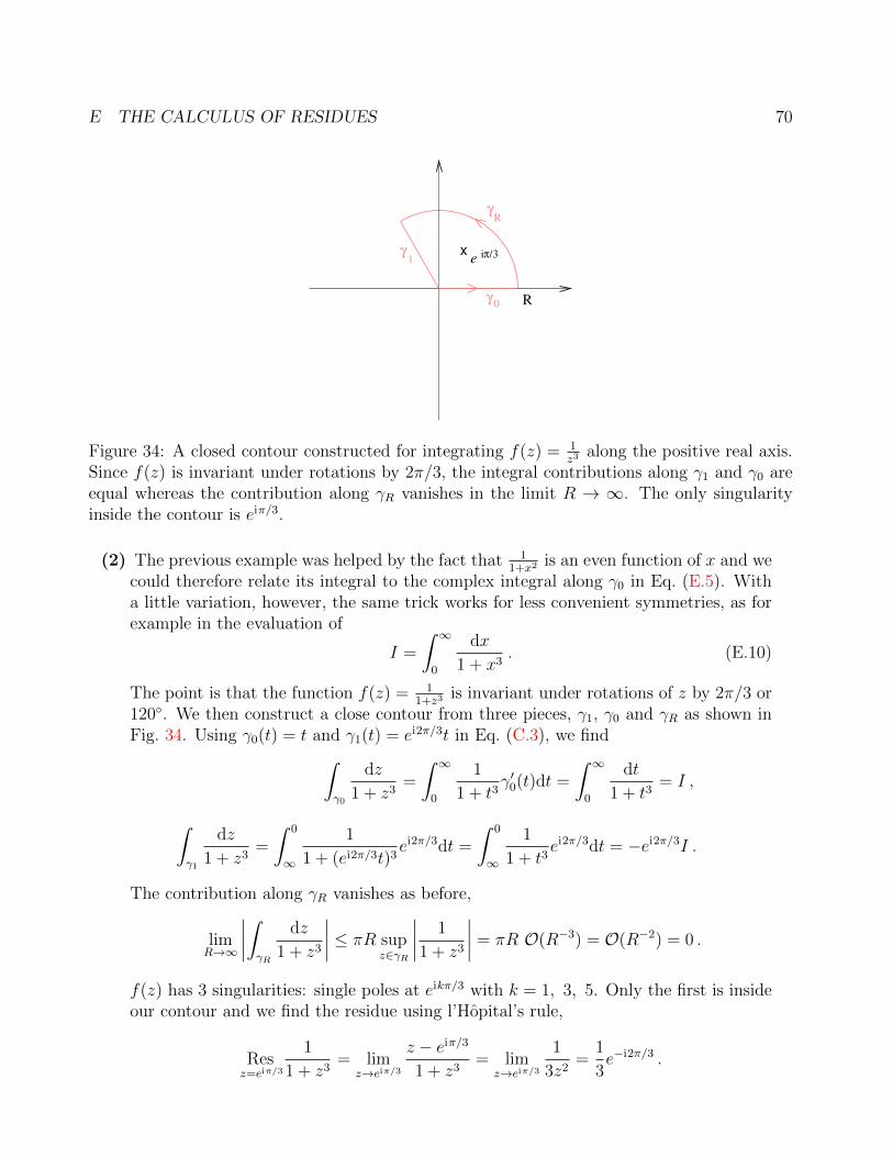
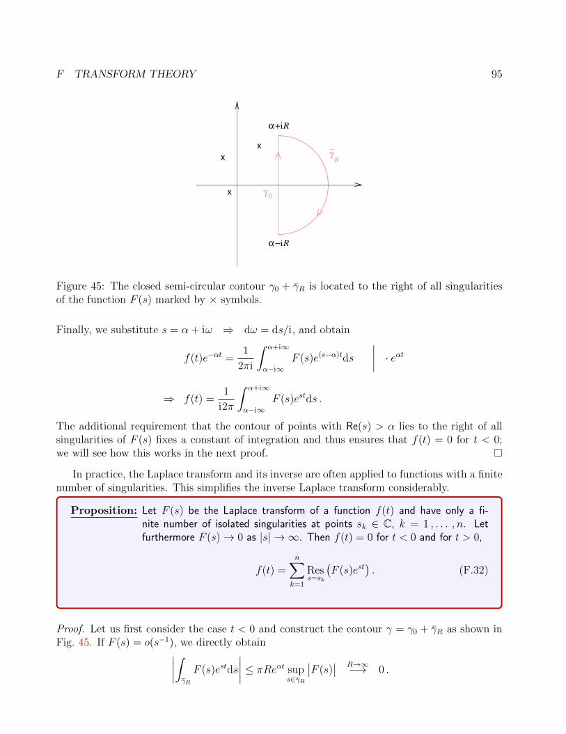
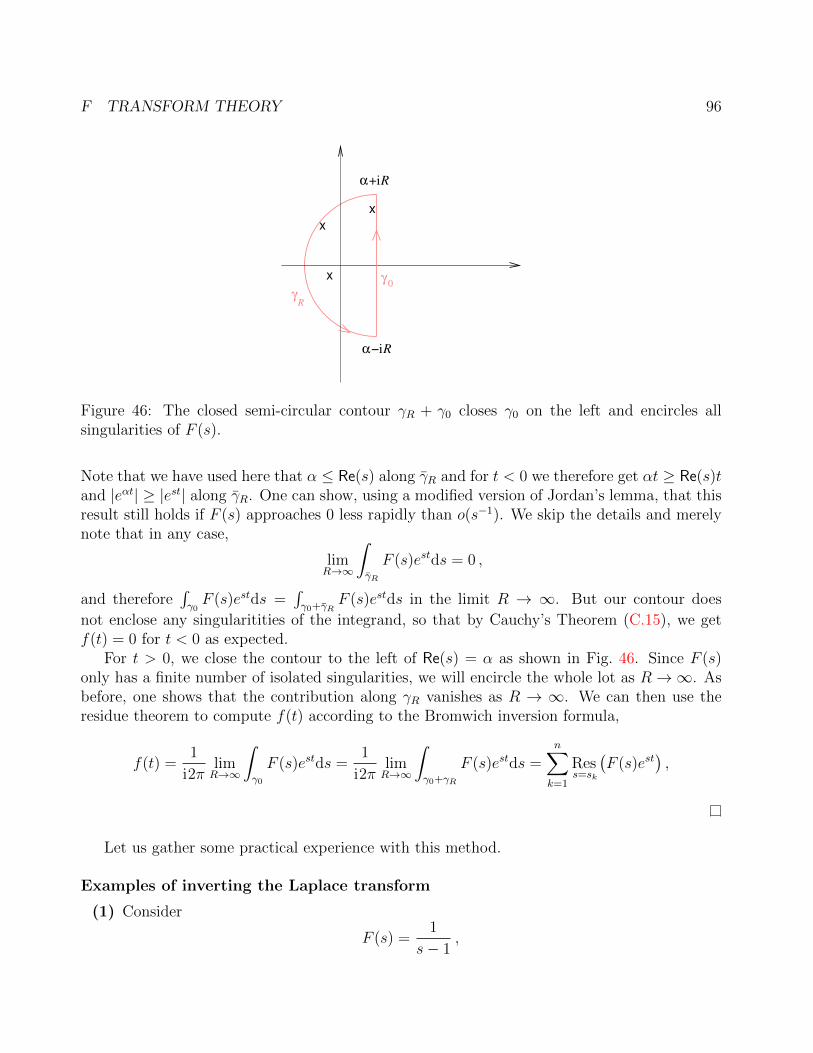
NST Part IB Complex Methods Lecture Notes Abstract This document contains the long version of the lecture notes for the IB course Complex Methods. These notes are extensive and written such that they can be consumed either together with the lecture or on their own. In drafting these notes, I am indebted to previous lecturers of this course and, in particular, the notes by R. E. Hunt (see also Dexter Chua’s site https://dec41.user.srcf.net/notes/) and Gary Gibbons. I also thank Owain Salter Fitz-Gibbon and Miren Radia for discussions and comments on the lecture notes. These notes assume that readers are already familiar with complex numbers, calculus in multi-dimensional real space R n , and Fourier transforms. The most important features of these three areas are briefly summarized, but not at the level of a dedicated lecture. This course is primarily aimed at applications of complex methods; readers interested in a more rigorous treatment of proofs are refered to the IB Complex Analysis lecture. Some more extensive discussions may also be found in the following books, though readers are not required to have studied them. • M. J. Ablowitz and A. S. Fokas, Complex variables: introduction and applications. Cambridge University Press (2003) • G. B. Arfken, H. J. Weber, and F. E. Harris, Mathematical Methods for Physicists. Elsevier (2013) • G. J. O. Jameson, A First Course in Complex Functions. Chapman and Hall (1970) • T. Needham, Visual complex analysis, Clarendon (1998) • H. A. Priestley, Introduction to Complex Analysis. Clarendon (1990) • K. F. Riley, M. P. Hobson, and S. J. Bence, Mathematical Methods for Physics and Engineering: a comprehensive guide. Cambridge University Press (2002) Example sheets will be on Moodle and on http://www.damtp.cam.ac.uk/user/examples Lectures Webpage: http://www.damtp.cam.ac.uk/user/us248/Lectures/lectures.html Cambridge, 15 Jan 2021 Ulrich Sperhake 1
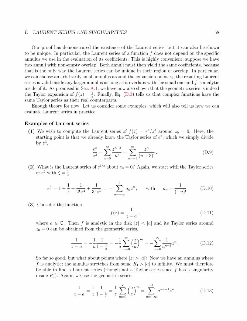
Transcript
NST Part IB Complex Methods
Lecture Notes
Abstract
This document contains the long version of the lecture notes for the IB course ComplexMethods. These notes are extensive and written such that they can be consumed eithertogether with the lecture or on their own. In drafting these notes, I am indebted toprevious lecturers of this course and, in particular, the notes by R. E. Hunt (see alsoDexter Chua’s site https://dec41.user.srcf.net/notes/) and Gary Gibbons. I alsothank Owain Salter Fitz-Gibbon and Miren Radia for discussions and comments on thelecture notes.
These notes assume that readers are already familiar with complex numbers, calculusin multi-dimensional real space Rn, and Fourier transforms. The most important featuresof these three areas are briefly summarized, but not at the level of a dedicated lecture.This course is primarily aimed at applications of complex methods; readers interested ina more rigorous treatment of proofs are refered to the IB Complex Analysis lecture. Somemore extensive discussions may also be found in the following books, though readers arenot required to have studied them.
• M. J. Ablowitz and A. S. Fokas, Complex variables: introduction and applications.Cambridge University Press (2003)
• G. B. Arfken, H. J. Weber, and F. E. Harris, Mathematical Methods for Physicists.Elsevier (2013)
• G. J. O. Jameson, A First Course in Complex Functions. Chapman and Hall (1970)
• T. Needham, Visual complex analysis, Clarendon (1998)
• H. A. Priestley, Introduction to Complex Analysis. Clarendon (1990)
• K. F. Riley, M. P. Hobson, and S. J. Bence, Mathematical Methods for Physics andEngineering: a comprehensive guide. Cambridge University Press (2002)
In this section, we briefly review some basic properties of general calculus, complex numbersand functions of them. While many readers will be familiar with the content of this section,it will serve as a convenient reference throughout these notes. We will also introduce somenotational conventions.
A.1 Complex numbers
We begin our discussion of complex numbers with the imaginary unit.
Def. : The “imaginary unit” is i ..=√−1 .
A complex number z ∈ C can then be written as
z = x+ iy = reiφ = r cosφ+ i r sinφ . (A.1)
We may regard (x, y) and (r, φ) as Cartesian and polar coordinates on the R2, respectively, andthey are related by the transformation
x = Re(z) = r cosφ , y = Im(z) = r sinφ ,
r = |z| =√x2 + y2 , φ = arg z , (A.2)
where Re() and Im() denote the real and imaginary part. The argument arg z is only definedup to integer multiples of 2π and we therefore define the following.
Def. : The “principal argument” of a complex number z is the value φ = arg z that fallsinto the range (−π, π].
One may be tempted to compute the argument of z = x+ iy from
φ = arctan(yx
), (A.3)
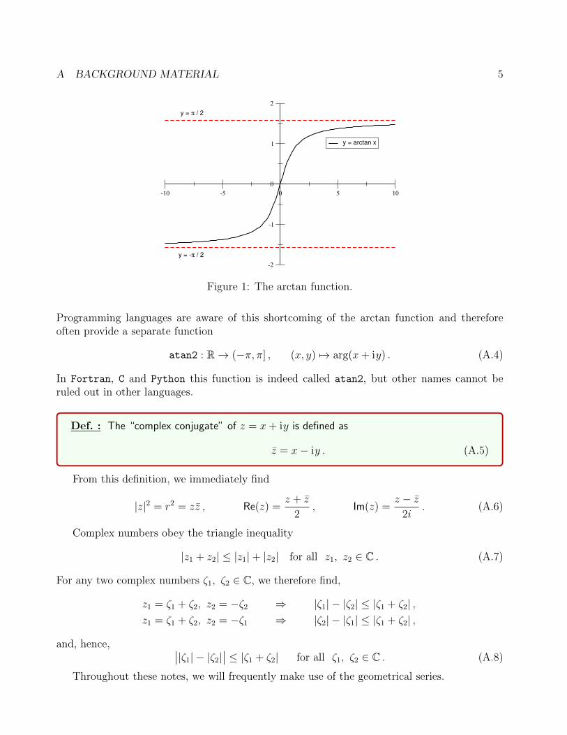
but this does not work because the arctan function only maps to the interval (−π/2, π/2)as illustrated in Fig. 1. The arctan function therefore returns the principle argument onlyfor points with positive real part but is off by π radians when Re(z) < 0. For example, forφ = argz = π/3,
z = cosφ+ i sinφ =1
2+ i
√3
2and arctan
y
x= arctan(
√3) =
π
3,
gives us the correct result, but for φ = argz = 2π/3, we obtain
z = cosφ+ i sinφ = −1
2+ i
√3
2and arctan
y
x= arctan(−
√3) = −π
3.
A BACKGROUND MATERIAL 5
-10 -5 0 5 10
-2
-1
0
1
2
y = arctan x
y = -π / 2
y = π / 2
Figure 1: The arctan function.
Programming languages are aware of this shortcoming of the arctan function and thereforeoften provide a separate function
atan2 : R→ (−π, π] , (x, y) 7→ arg(x+ iy) . (A.4)
In Fortran, C and Python this function is indeed called atan2, but other names cannot beruled out in other languages.
Def. : The “complex conjugate” of z = x+ iy is defined as
z = x− iy . (A.5)
From this definition, we immediately find
|z|2 = r2 = zz , Re(z) =z + z
2, Im(z) =
z − z2i
. (A.6)
Complex numbers obey the triangle inequality
|z1 + z2| ≤ |z1|+ |z2| for all z1, z2 ∈ C . (A.7)
For any two complex numbers ζ1, ζ2 ∈ C, we therefore find,
and, hence, ∣∣|ζ1| − |ζ2|∣∣ ≤ |ζ1 + ζ2| for all ζ1, ζ2 ∈ C . (A.8)
Throughout these notes, we will frequently make use of the geometrical series.
A BACKGROUND MATERIAL 6
Proposition: For z ∈ C, z 6= 1 and n ∈ N0,
n∑k=0
zk =1− zn+1
1− z . (A.9)
Proof. We proof this by induction. Evidently, for n = 0, we have z0 = 1 = (1− z)/(1− z). Solet us assume Eq. (A.9) holds for n. Then
n+1∑k=0
zk = zn+1 +n∑k=0
zk = zn+1 +1− zn+1
1− z =zn+1 − zn+2 + 1− zn+1
1− z =1− zn+2
1− z
Note that Eq. (A.9) is correct for any z 6= 1, irrespective of whether or not the seriesconverges. For |z| < 1, we furthermore obtain the limit
∞∑k=0
zk =1
1− z . (A.10)
As we shall see later, this equation may also be interpreted as the Taylor expansion of thefunction 1/(1− z) around z = 0.
Finally, let us recall the definition of open sets. Equation (A.2) provides us with a norm onC and we can define,
Def. : A set D ⊂ C is an open set if for all z0 ∈ D, there exist a ε > 0 such that the εsphere of points with |z − z0| < ε is contained in D. More prosaically, an open setdoes not contain its boundary.
Def. : A “neighbourhood of a point z ∈ C” is an open set D that contains the point z.
A.2 Trigonometric and hyperbolic functions
Complex numbers provide a close connection between trigonometric and hyperbolic functionsthrough the relations
eiφ = cosφ+ i sinφ ∧ e−iφ = cosφ− i sinφ
⇔ cosφ =eiφ + e−iφ
2∧ sinφ =
eiφ − e−iφ
2i. (A.11)
A BACKGROUND MATERIAL 7
Trigonometric functions satisfy a vast range of relations and an impressive collection can befound on [7]. Here we list a few that will be used later on,
cos(α + β) = cosα cos β − sinα sin β , (A.12)
sin(α + β) = sinα cos β + cosα sin β , (A.13)
cos(θ ± π
2
)= ∓ sin θ , cos(θ + π) = − cos θ , cos(θ + 2kπ) = cos θ , (A.14)
sin(θ ± π
2
)= ± sin θ , sin(θ + π) = − sin θ , sin(θ + 2kπ) = sin θ , (A.15)
where k ∈ Z. The hyperbolic functions are given by
coshφ =eφ + e−φ
2∧ sinhφ =
eφ − e−φ2
.
⇔ eφ = coshφ+ sinhφ ∧ e−φ = coshφ− sinhφ . (A.16)
Equations (A.11) and (A.16) imply
cos(ix) =e−x + ex
2= coshx ⇔ cosh(ix) = cos(−x) = cos x , (A.17)
sin(ix) =e−x − ex
2i= i sinhx ⇔ sinh(ix) = i sinx . (A.18)
Similar relations can be established for tan, cot, tanh, coth etc., but these are all direct conse-quences of Eqs. (A.17) and (A.18).
The hyperbolic functions satisfy addition theorems analogous to (A.12) and (A.13),
cosh(x+ y) = coshx cosh y + sinh y sinhx , (A.19)
sinh(x+ y) = sinh x cosh y + coshx sinh y . (A.20)
A.3 Calculus of real functions in ≥ 1 variables
We shall occasionally regard a function of a complex variable as a function of two real vari-ables, the real and imaginary parts x = Re(z), y = Im(z). The partial derivative ∂f/∂xi isdefined in the usual way keeping all the other xj constant. For an open subset Ω ∈ Rn, we define
Def. : Cm(Ω) is the set of all functions f : Ω⇒ R whose partial derivatives up to order mexist and are continuous.
Note that the existence of the partial derivatives is not a particularly strong requirement.In fact, it does not even imply that the function f is continuous.
A BACKGROUND MATERIAL 8
Example : Let
f(x, y) =
x for y = 0y for x = 0arbitrary for x 6= 0 and y 6= 0
(A.21)
We immediately find satisfactory partial derivatives at the origin,
∂f
∂x(0, 0) = 1 =
∂f
∂y(0, 0) . (A.22)
Differentiability of a function f on Ω ⊂ Rn is a stronger criterion that can be defined asfollows.
Def. : A function f : Ω → R is differentiable if there exists a linear function A : Rn → Rsuch that for every x ∈ Ω
f(x + ∆x)− f(x) = A(∆x) + r(∆x) with lim∆x→0
r(∆x)
||∆x|| = 0 . (A.23)
Furthermore, this definition extends to vector-valued functions f : Ω→ Rm by simplyconsidering each component function fi separately.
Finally, the function f is continuously differentiable if furthermore f ∈ C1, i.e. if itsfirst partial derivatives are continuous.
One can then show that the following implications (but in general not their reverse!) hold,
f is continuously differentiable ⇔ all partial derivatives∂fi∂xj
are continuous
⇒ f is differentiable
⇒ f is continuous and all partial derivatives∂fi∂xj
exist . (A.24)
For our purposes, the important consequence is that continuity of the partial derivatives ∂fi/∂xjis sufficient to ensure all differentiable properties we may require from our function f .
We next recapitulate some properties of sequences and series of functions.
Def. : Let fk : Ω ⊆ Rn → R, k ∈ N be a sequence of functions. The sequence fn isuniformly convergent on Ω with limit f : Ω→ R if
∀ε>0 ∃N∈N ∀k≥N, x∈Ω |fk(x)− f(x)| < ε . (A.25)
One can show that for a uniformly converging sequence of functions fn : R→ R,
limn→∞
∫ b
a
fn(x)dx =
∫ b
a
f(x)dx . (A.26)
A BACKGROUND MATERIAL 9
Uniform convergence of complex functions is defined in complete analogy. The geometric series(A.10), for example, is uniformly convergent in C for |z| < 1. This will become important inour derivation of the Laurent series in Sec. D.1, where we need to swap the integral and thesum.
B ANALYTIC FUNCTIONS 10
B Analytic functions
B.1 The Extended Complex Plane and the Riemann Sphere
In Sec. A.1, we have seen that a complex number z is defined in terms of its real and imaginaryparts (x, y). This mapping z ↔ (x, y) is bijective and we can therefore identify the complexplane with the 2-dimensional plane of ordered pairs of real numbers. We can likewise identifyaddition and multiplication and summarize this in the following definition.
Def. : We denote the set of all complex numbers by C. A complex number z = x + iy isuniquely identified with a pair of real numbers (x, y) ∈ R2.We can furthermore represent addition and multiplication of two complex numbersz1 = x1 + iy1, z2 = x2 + iy2 as operations on R2 according to
The identification of C with R2 can sometimes be helpful, but we will not carry it too far; afterall, much of the beauty of complex numbers arises from treating them as numbers in their ownright.
It is often convenient to include ∞ as part of the complex domain and therefore define:
Def. : The extended complex domain is C∗ = C ∪ ∞ .
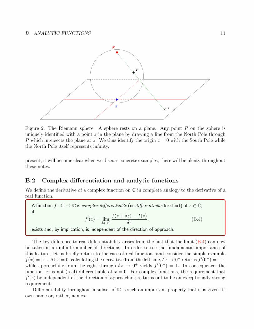
The fact that∞ is indeed a single point is best understood in terms of the Riemann spherewhich we display in Fig. 2. There we consider a sphere resting on the complex plane. A bijectivemapping between points P on the sphere and points z in the plane is obtained by drawing aline from the North Pole through P until it intersects the plane; the point of intersection isz. The origin z = 0 is thus identified with the South Pole and we reach infinity by moving Pever closer to the North Pole which represents z =∞. In particular, infinity represents merelyone single point and we reach the same point by going towards infinity in any direction. Thesymbols ∞ and −∞ therefore denote the same point in C∗ and we will only use the expression−∞ if we wish to emphasize that we proceed towards infinity in a specific direction, namelyalong the negative real axis. The Riemann sphere may appear as a nice but impractical device,but we will soon encounter a very useful application.
An alternative viewpoint of great value for investigating properties of infinity consists inthe substitution ζ = 1/z. We then ascribe to a function f(z) a specific property at z = ∞, ifthe function f(1/ζ) has this property at ζ = 0. If this procedure appears somewhat vague at
B ANALYTIC FUNCTIONS 11
S
N
z
P
Figure 2: The Riemann sphere. A sphere rests on a plane. Any point P on the sphere isuniquely identified with a point z in the plane by drawing a line from the North Pole throughP which intersects the plane at z. We thus identify the origin z = 0 with the South Pole whilethe North Pole itself represents infinity.
present, it will become clear when we discuss concrete examples; there will be plenty throughoutthese notes.
B.2 Complex differentiation and analytic functions
We define the derivative of a complex function on C in complete analogy to the derivative of areal function.
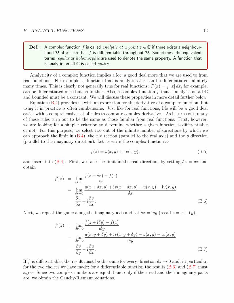
A function f : C→ C is complex differentiable (or differentiable for short) at z ∈ C,if
f ′(z) = limδz→0
f(z + δz)− f(z)
δz, (B.4)
exists and, by implication, is independent of the direction of approach.
The key difference to real differentiability arises from the fact that the limit (B.4) can nowbe taken in an infinite number of directions. In order to see the fundamental importance ofthis feature, let us briefly return to the case of real functions and consider the simple examplef(x) = |x|. At x = 0, calculating the derivative from the left side, δx→ 0− returns f ′(0−) = −1,while approaching from the right through δx → 0+ yields f ′(0+) = 1. In consequence, thefunction |x| is not (real) differentiable at x = 0. For complex functions, the requirement thatf ′(z) be independent of the direction of approaching z, turns out to be an exceptionally strongrequirement.
Differentiability throughout a subset of C is such an important property that it is given itsown name or, rather, names.
B ANALYTIC FUNCTIONS 12
Def. : A complex function f is called analytic at a point z ∈ C if there exists a neighbour-hood D of z such that f is differentiable throughout D. Sometimes, the equivalentterms regular or holomorphic are used to denote the same property. A function thatis analytic on all C is called entire.
Analyticity of a complex function implies a lot; a good deal more that we are used to fromreal functions. For example, a function that is analytic at z can be differentiated infinitelymany times. This is clearly not generally true for real functions: F (x) =
∫|x| dx, for example,
can be differentiated once but no further. Also, a complex function f that is analytic on all Cand bounded must be a constant. We will discuss these properties in more detail further below.
Equation (B.4) provides us with an expression for the derivative of a complex function, butusing it in practice is often cumbersome. Just like for real functions, life will be a good dealeasier with a comprehensive set of rules to compute complex derivatives. As it turns out, manyof these rules turn out to be the same as those familiar from real functions. First, however,we are looking for a simpler criterion to determine whether a given function is differentiableor not. For this purpose, we select two out of the infinite number of directions by which wecan approach the limit in (B.4), the x direction (parallel to the real axis) and the y direction(parallel to the imaginary direction). Let us write the complex function as
f(z) = u(x, y) + i v(x, y) , (B.5)
and insert into (B.4). First, we take the limit in the real direction, by setting δz = δx andobtain
f ′(z) = limδx→0
f(z + δx)− f(z)
δx
= limδx→0
u(x+ δx, y) + iv(x+ δx, y)− u(x, y)− iv(x, y)
δx
=∂u
∂x+ i
∂v
∂x. (B.6)
Next, we repeat the game along the imaginary axis and set δz = iδy (recall z = x+ i y),
f ′(z) = limδy→0
f(z + iδy)− f(z)
iδy
= limδy→0
u(x, y + δy) + iv(x, y + δy)− u(x, y)− iv(x, y)
iδy
=∂v
∂y− i
∂u
∂x. (B.7)
If f is differentiable, the result must be the same for every direction δz → 0 and, in particular,for the two choices we have made; for a differentiable function the results (B.6) and (B.7) mustagree. Since two complex numbers are equal if and only if their real and their imaginary partsare, we obtain the Cauchy-Riemann equations,
B ANALYTIC FUNCTIONS 13
Def. : For a complex function f(z) = u(x, y) + iv(x, y), the Cauchy-Riemann equationsare
∂u
∂x=∂v
∂y,
∂u
∂y= −∂v
∂x, (B.8)
and have proven the following result,
Proposition: If f(z) = u(x, y) + iv(x, y) is differentiable at z = z0, it satisfies the Cauchy-Riemann equations (B.8) at this point.
The Cauchy-Riemann equations thus constitute a necessary condition for differentiability.Are they also sufficient? In general, no. For the reverse implication to be true, we also needto demand that u and v are themselves differentiable functions, and we have seen in Sec. A.3that differentiability of u and v is a stronger condition than the mere existence of their partialderivatives ux, uy, vx, vy. We have also seen, however, that u and v are differentiable if theirpartial derivatives exist and are continuous. This provides us with a practical criterion forassessing the differentiability of a complex function.
Proposition: If a function f(z) = u(x, y) + iv(x, y) satisfies
∂u
∂x=∂v
∂y,
∂u
∂y= −∂v
∂x,
at a point z = z0 and the partial derivatives are continuous in a neighbourhoodof z0, then f(z) is differentiable at z = z0.
The complete proof of this result is outside the scope of our course, but will be discussedin the IB Complex Analysis lecture.
Our discussion of the differentiability conditions for a complex function has been based onwriting
f(z) = u(x, y) + iv(x, y) , z = x+ iy , (B.9)
and considering the differentiability of the functions u and v. An alternative and equivalentapproach consists in recalling the complex conjugate z and the relations
x =z + z
2, y =
z − z2i
= −iz − z
2. (B.10)
This allows us to write any complex function in the form g(z, z) and it turns out that g isdifferentiable if it does not depend on z, i.e. ∂g/∂z = 0. This will be explored in more detailin the first example sheet.
Complex differentiation obeys the product, quotient and chain rule we are already familiarwith from real calculus.
B ANALYTIC FUNCTIONS 14
Corollary: “Product rule”: The product of two analytic functions f g is analytic with thederivative
(f g)′(z) = f ′(z) g(z) + f(z) g′(z) . (B.11)
Proof. Given that f and g are differentiable, we can directly evaluate the derivative of theproduct fg from Eq. (B.4). We first define
$ ..=f(z + h)− f(z)
h− f ′(z) ,
w ..=g(z + h)− g(z)
h− g′(z) ,
Note that both $ → 0 and w → 0 as h→ 0. It follows that
The use of the Cauchy-Riemann conditions is best illustrated with some examples of ana-lytic and non-analytic functions.
Examples of analytic functions
(1) The function f(z) = z is entire, i.e. analytic everywhere. Here, we have u(x, y) = xand v(x, y) = y and the Cauchy-Riemann conditions
∂u
∂x= 1 =
∂v
∂y,
∂u
∂y= 0 = −∂v
∂y,
are satisfied everywhere. Furthermore, the partial derivatives are clearly continuous.Alternatively, we could have plugged f(z) = z directly into Eq. (B.4) to prove itsdifferentiability which also gives us directly f ′(z) = 1.
(2) The function ez = ex(cos y + i sin y) is also entire, since
∂u
∂x= ex cos y =
∂v
∂y,
∂u
∂y= −ex sin y = −∂v
∂x(B.14)
Again, the partial derivatives are continuous everywhere. Having demonstrated itsdifferentiability, we are free to compute the derivative f ′ along any direction we like.We choose the x direction in Eq. (B.4) and obtain
f ′(z) =∂u
∂x+ i
∂v
∂x= ex cos y + iex sin y = ex eiy = ez , (B.15)
as expected.
(3) For n ∈ N, the function f(z) = zn is also entire. One could check this by writingzn = rn(cos θ + i sin θ)n which leads to u = rn cos(nθ) and v = rn sin(nθ), but thisbecomes rather cumbersome since we still need to switch from polar to Cartesiancoordinates. A simpler proof uses induction to show f ′(z) = nzn−1. We have done thisalready for n = 1 in item (1) above. Let’s assume then the result is true for n. Wethen write
(z + δz)n+1 − zn+1
δz=
(z + δz)n(z + δz)− zn(z + δz) + znδz
δz
= (z + δz)(z + δz)n − zn
δz+ zn
and therefore
f ′(z) = limδz→0
(z + δz)n+1 − zn+1
δz= z nzn−1 + zn = (n+ 1)zn . (B.16)
Since a linear combination αf + βg, α, β ∈ C of two analytic functions f and g ismanifestly analytic by the definition (B.4), polynomials are also entire functions.
B ANALYTIC FUNCTIONS 16
(4) The function f(z) = 1/z is analytic everywhere except at z = 0. Writing
f(z) =1
z=
z
zz=
x− iy
x2 + y2, (B.17)
we find
∂xu =y2 − x2
(x2 + y2)2, ∂yu =
−2xy
(x2 + y2)2, ∂xv =
2xy
(x2 + y2)2, ∂yv =
y2 − x2
(x2 + y2)2,
and the Cauchy-Riemann conditions hold everywhere except at the origin. Further-more, the partial derivatives are continuous in R2 \ (0, 0). We evaluate f ′ along thex direction using differentiation rules for real functions,
∂
∂x
x− iy
x2 + y2=−x2 + y2 + 2ixy
(x2 + y2)2=
(ix+ y)2
(x2 + y2)2=−(x− iy)2
(x2 + y2)2= − z2
z2z2= − 1
z2.
Combined with the product and chain rule, this result furthermore gives us the quotientrule, (f/g)′ = (f ′ g−g′ f)/g2 which, for analytic functions f and g, is analytic provided
g(z) 6= 0. We furthermore conclude that any rational function f(x) = P (z)Q(z)
, where P
and Q are polynomials, is analytic except at points where Q(z) = 0. For example,
f(z) =z
z2 + 1, (B.18)
is analytic everywhere except z = ±i.
(5) Many standard functions turn out to have the same derivatives when extended to thecomplex domain. The most important examples are as follows.
The quotient rule gives us (tan)′(z) = 1/ cos2 z, though this is analytic only atpoints where cos z 6= 0. Useful expressions for the cos and sin functions in termsof (x, y) are obtained from the addition theorems (A.12) and (A.13),
sin z = sin(x+ iy) = sinx cos(iy) + cos x sin(iy) = sin x cosh y + i cos x sinh y ,
cos z = cos(x+ iy) = cos x cos(iy)− sinx sin(iy) = cos x cosh y − i sin x sinh y .
(B.21)
• Similarly, the hyperbolic functions cosh, sinh etc. differentiate as expected, cosh′ =sinh, sinh′ = cosh.
B ANALYTIC FUNCTIONS 17
• The logarithm f(z) = log z = log |z|+ i arg z has derivative 1z; we will discuss the
logarithm in more detail in Sec. B.4 under the heading of multi-valued functionsand branch cuts.
It is also instructive to consider non-analytic functions and see how this is reflected in theCauchy-Riemann conditions. Some examples are given in the following.
Examples of non-analytic functions
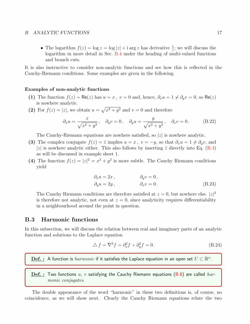
(1) The function f(z) = Re(z) has u = x , v = 0 and, hence, ∂xu = 1 6= ∂yv = 0, so Re(z)is nowhere analytic.
(2) For f(z) = |z|, we obtain u =√x2 + y2 and v = 0 and therefore
∂xu =x√
x2 + y2, ∂yv = 0 , ∂yu =
y√x2 + y2
, ∂xv = 0 . (B.22)
The Cauchy-Riemann equations are nowhere satisfied, so |z| is nowhere analytic.
(3) The complex conjugate f(z) = z implies u = x , v = −y, so that ∂xu = 1 6= ∂yv, and|z| is nowhere analytic either. This also follows by inserting z directly into Eq. (B.4)as will be discussed in example sheet 1.
(4) The function f(z) = |z|2 = x2 + y2 is more subtle. The Cauchy Riemann conditionsyield
∂xu = 2x , ∂yv = 0 ,
∂yu = 2y , ∂xv = 0 . (B.23)
The Cauchy Riemann conditions are therefore satisfied at z = 0, but nowhere else. |z|2is therefore not analytic, not even at z = 0, since analyticity requires differentiabilityin a neighbourhood around the point in question.
B.3 Harmonic functions
In this subsection, we will discuss the relation between real and imaginary parts of an analyticfunction and solutions to the Laplace equation
4 f = ∇2f = ∂2xf + ∂2
yf = 0 . (B.24)
Def. : A function is harmonic if it satisfies the Laplace equation in an open set U ⊂ Rn.
Def. : Two functions u, v satisfying the Cauchy Riemann equations (B.8) are called har-monic conjugates.
The double appearance of the word “harmonic” in these two definitions is, of course, nocoincidence, as we will show next. Clearly the Cauchy Riemann equations relate the two
B ANALYTIC FUNCTIONS 18
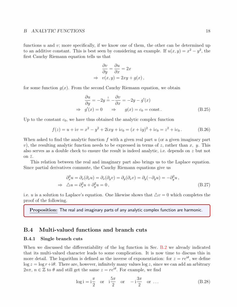
functions u and v; more specifically, if we know one of them, the other can be determined upto an additive constant. This is best seen by considering an example. If u(x, y) = x2 − y2, thefirst Cauchy Riemann equation tells us that
∂v
∂y=∂u
∂x= 2x
⇒ v(x, y) = 2xy + g(x) ,
for some function g(x). From the second Cauchy Riemann equation, we obtain
∂u
∂y= −2y
!= −∂v
∂x= −2y − g′(x)
⇒ g′(x) = 0 ⇒ g(x) = c0 = const . (B.25)
Up to the constant c0, we have thus obtained the analytic complex function
When asked to find the analytic function f with a given real part u (or a given imaginary partv), the resulting analytic function needs to be expressed in terms of z, rather than x, y. Thisalso serves as a double check to ensure the result is indeed analytic, i.e. depends on z but noton z.
This relation between the real and imaginary part also brings us to the Laplace equation.Since partial derivatives commute, the Cauchy Riemann equations give us
i.e. u is a solution to Laplace’s equation. One likewise shows that 4v = 0 which completes theproof of the following.
Proposition: The real and imaginary parts of any analytic complex function are harmonic.
B.4 Multi-valued functions and branch cuts
B.4.1 Single branch cuts
When we discussed the differentiability of the log function in Sec. B.2 we already indicatedthat its multi-valued character leads to some complication. It is now time to discuss this inmore detail. The logarithm is defined as the inverse of exponentiation: for z = reiθ, we definelog z = log r+iθ. There are, however, infinitely many values log z, since we can add an arbitrary2nπ, n ∈ Z to θ and still get the same z = reiθ. For example, we find
log i = iπ
2or i
5π
2or − i
3π
2or . . . (B.28)
B ANALYTIC FUNCTIONS 19
x
y
x
θ
z
C3
C
2C
1
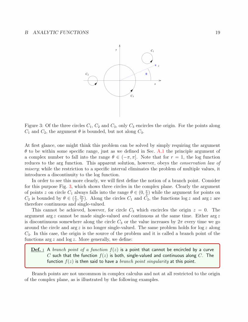
Figure 3: Of the three circles C1, C2 and C3, only C3 encircles the origin. For the points alongC1 and C2, the argument θ is bounded, but not along C3.
At first glance, one might think this problem can be solved by simply requiring the argumentθ to be within some specific range, just as we defined in Sec. A.1 the principle argument ofa complex number to fall into the range θ ∈ (−π, π]. Note that for r = 1, the log functionreduces to the arg function. This apparent solution, however, obeys the conservation law ofmisery; while the restriction to a specific interval eliminates the problem of multiple values, itintroduces a discontinuity to the log function.
In order to see this more clearly, we will first define the notion of a branch point. Considerfor this purpose Fig. 3, which shows three circles in the complex plane. Clearly the argumentof points z on circle C1 always falls into the range θ ∈ (0, π
2) while the argument for points on
C2 is bounded by θ ∈ (π2, 3π
2). Along the circles C1 and C2, the functions log z and arg z are
therefore continuous and single-valued.This cannot be achieved, however, for circle C3 which encircles the origin z = 0. The
argument arg z cannot be made single-valued and continuous at the same time. Either arg zis discontinuous somewhere along the circle C3 or the value increases by 2π every time we goaround the circle and arg z is no longer single-valued. The same problem holds for log z alongC3. In this case, the origin is the source of the problem and it is called a branch point of thefunctions arg z and log z. More generally, we define:
Def. : A branch point of a function f(z) is a point that cannot be encircled by a curveC such that the function f(z) is both, single-valued and continuous along C. Thefunction f(z) is then said to have a branch point singularity at this point.
Branch points are not uncommon in complex calculus and not at all restricted to the originof the complex plane, as is illustrated by the following examples.
B ANALYTIC FUNCTIONS 20
Examples of branch points
(1) The function log(z − a), a = const ∈ C, has a branch point at z = a.
(2) f(z) = log(z−1z+1
)= log(z − 1)− log(z + 1) has two branch points at ±1.
(3) The function f(z) = zα = rαeiαθ, α = const is more complicated. Consider a circle ofradius r0 around the origin and let us start at θ = 0 where we have f = rα0 . Now goaround the circle once; as we approach θ = 2π, we find f = rα0 e
iα2π which is equal toour starting value only if
eiα2π = 1 ⇔ α2π = 2nπ ⇔ α ∈ Z , (B.29)
i.e. for integer values of α. For non-integer α, the function zα has a branch point atthe origin.
(4) Recall that we extended the complex domain by including ∞ and that we planned tostudy the behaviour of functions at z = ∞ by considering the behaviour of f(z = 1
ζ)
at ζ = 0. In this case, log z has a branchpoint at z =∞ if log 1ζ
has a branch point at
ζ = 0. This is indeed the case, since log 1ζ
= − log ζ and the latter has a branch point
at ζ = 0. We likewise show that f(z) = zα has a branch point at z =∞ for α /∈ Z.
(5) Sometimes, we may think at first glance that a function has a specific branch pointwhen in fact it does not. For example, the function f(z) = log
(z−1z+1
)does not have a
branch point at infinity. With z = 1/ζ, we find
f(z = 1/ζ) = log
(z − 1
z + 1
)= log
(1− ζ1 + ζ
).
For ζ close to zero, 1−ζ1+ζ
stays close to 1 and thus stays clear of the branch point 0of the log function; in other words, we can encircle ζ = 0 without encountering anydiscontinuity of log 1−ζ
1+ζalong the curve.
Having identified the potentially problematic branch points, the obvious questions is how wecan handle them. The answer are branch cuts.
In order to obtain single-valued and continuous functions, we need to constrain the regimeof the complex domain we are allowed to consider; more specifically, we must exclude curvesthat encircle branch points. For the log z function, this means we have to prevent curves fromencircling the origin and this is achieved by drawing a red line, a branch cut which no curve isallowed to cross. For the function f(z) = log z, for example, we can introduce a branch cut alongthe nonpositive real axis as shown in Fig. 4. Once we have decided where to place the branchcut, we can specify the range the argument θ is allowed to take, for example θ ∈ (−π, π]. Thisdefines a branch of the function log z and on this branch, log z is single-valued and continuousalong any curve that does not cross the branch cut. This branch of log z is furthermore analyticeverywhere with derivative d
dzlog z = 1
zexcept on the nonpositive real axis, where this branch
is not even continuous. Let us take a closer look at this discontinuity. For points just below thebranch cut, we have θ = −π + ε where 0 < ε 1 and therefore log z = log r0 − i(π − ε). Forpoints just above the branch cut, we have θ = π− ε and log z = log r0 + i(π− ε). The functionlog z therefore jumps by i2π across the cut, as expected.
B ANALYTIC FUNCTIONS 21
θ
x
z
x
y
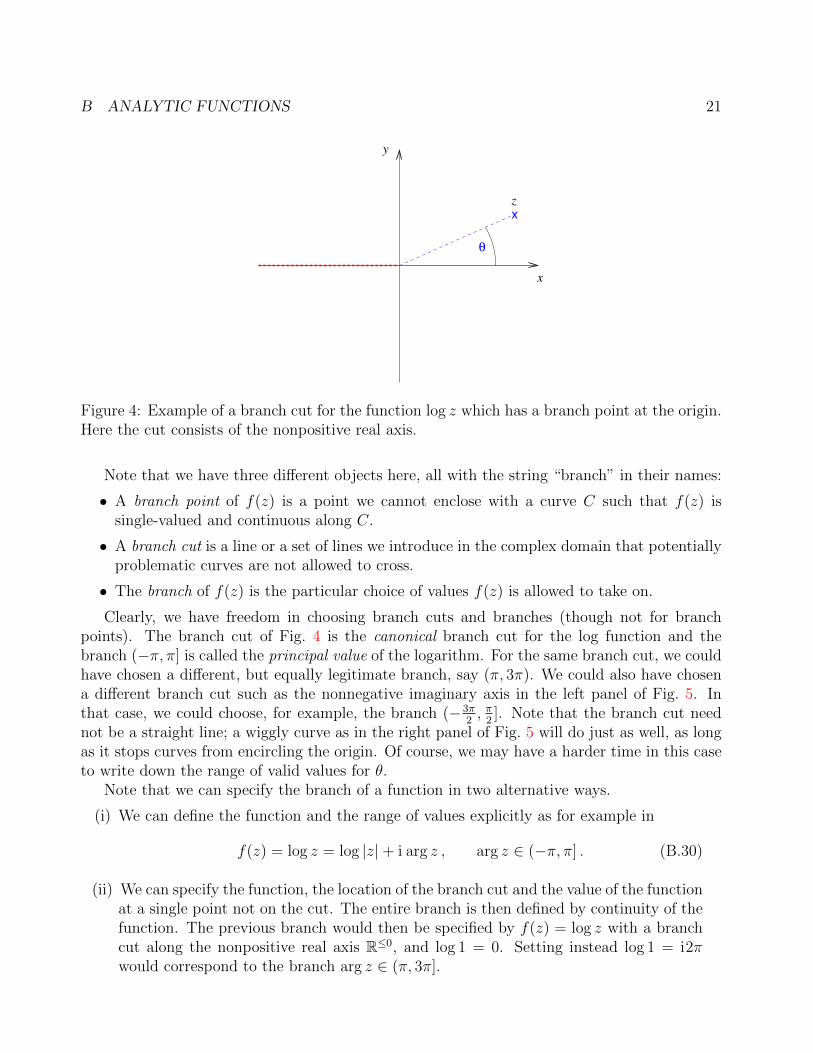
Figure 4: Example of a branch cut for the function log z which has a branch point at the origin.Here the cut consists of the nonpositive real axis.
Note that we have three different objects here, all with the string “branch” in their names:
• A branch point of f(z) is a point we cannot enclose with a curve C such that f(z) issingle-valued and continuous along C.
• A branch cut is a line or a set of lines we introduce in the complex domain that potentiallyproblematic curves are not allowed to cross.
• The branch of f(z) is the particular choice of values f(z) is allowed to take on.
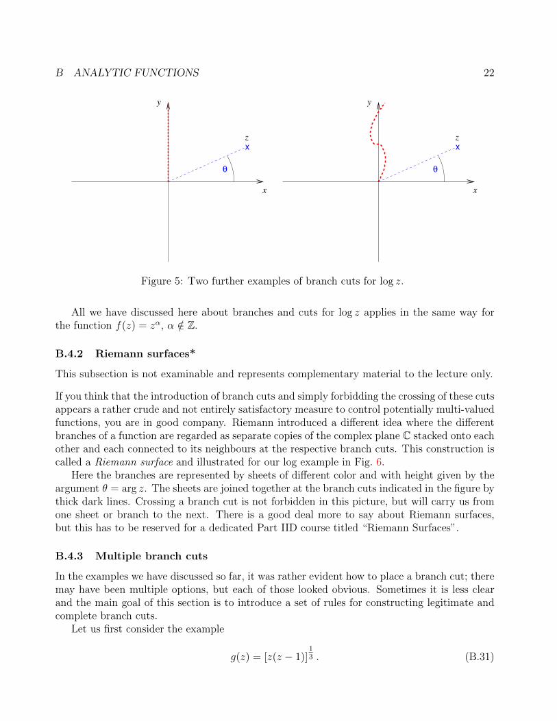
Clearly, we have freedom in choosing branch cuts and branches (though not for branchpoints). The branch cut of Fig. 4 is the canonical branch cut for the log function and thebranch (−π, π] is called the principal value of the logarithm. For the same branch cut, we couldhave chosen a different, but equally legitimate branch, say (π, 3π). We could also have chosena different branch cut such as the nonnegative imaginary axis in the left panel of Fig. 5. Inthat case, we could choose, for example, the branch (−3π
2, π
2]. Note that the branch cut need
not be a straight line; a wiggly curve as in the right panel of Fig. 5 will do just as well, as longas it stops curves from encircling the origin. Of course, we may have a harder time in this caseto write down the range of valid values for θ.
Note that we can specify the branch of a function in two alternative ways.
(i) We can define the function and the range of values explicitly as for example in
f(z) = log z = log |z|+ i arg z , arg z ∈ (−π, π] . (B.30)
(ii) We can specify the function, the location of the branch cut and the value of the functionat a single point not on the cut. The entire branch is then defined by continuity of thefunction. The previous branch would then be specified by f(z) = log z with a branchcut along the nonpositive real axis R≤0, and log 1 = 0. Setting instead log 1 = i2πwould correspond to the branch arg z ∈ (π, 3π].
B ANALYTIC FUNCTIONS 22
θ
x
z
x
y
θ
x
z
x
y
Figure 5: Two further examples of branch cuts for log z.
All we have discussed here about branches and cuts for log z applies in the same way forthe function f(z) = zα, α /∈ Z.
B.4.2 Riemann surfaces*
This subsection is not examinable and represents complementary material to the lecture only.
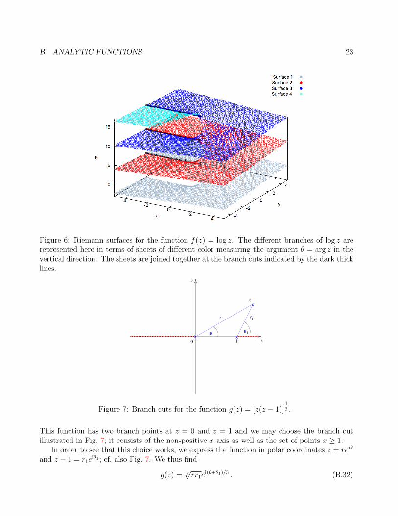
If you think that the introduction of branch cuts and simply forbidding the crossing of these cutsappears a rather crude and not entirely satisfactory measure to control potentially multi-valuedfunctions, you are in good company. Riemann introduced a different idea where the differentbranches of a function are regarded as separate copies of the complex plane C stacked onto eachother and each connected to its neighbours at the respective branch cuts. This construction iscalled a Riemann surface and illustrated for our log example in Fig. 6.
Here the branches are represented by sheets of different color and with height given by theargument θ = arg z. The sheets are joined together at the branch cuts indicated in the figure bythick dark lines. Crossing a branch cut is not forbidden in this picture, but will carry us fromone sheet or branch to the next. There is a good deal more to say about Riemann surfaces,but this has to be reserved for a dedicated Part IID course titled “Riemann Surfaces”.
B.4.3 Multiple branch cuts
In the examples we have discussed so far, it was rather evident how to place a branch cut; theremay have been multiple options, but each of those looked obvious. Sometimes it is less clearand the main goal of this section is to introduce a set of rules for constructing legitimate andcomplete branch cuts.
Let us first consider the example
g(z) = [z(z − 1)]13 . (B.31)
B ANALYTIC FUNCTIONS 23
Figure 6: Riemann surfaces for the function f(z) = log z. The different branches of log z arerepresented here in terms of sheets of different color measuring the argument θ = arg z in thevertical direction. The sheets are joined together at the branch cuts indicated by the dark thicklines.
θ
x
z
x x
0 1 x
y
θ1
r r1
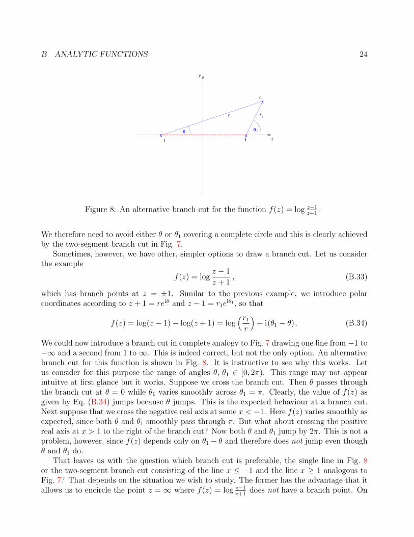
Figure 7: Branch cuts for the function g(z) = [z(z − 1)]13 .
This function has two branch points at z = 0 and z = 1 and we may choose the branch cutillustrated in Fig. 7; it consists of the non-positive x axis as well as the set of points x ≥ 1.
In order to see that this choice works, we express the function in polar coordinates z = reiθ
and z − 1 = r1eiθ1 ; cf. also Fig. 7. We thus find
g(z) = 3√rr1e
i(θ+θ1)/3 . (B.32)
B ANALYTIC FUNCTIONS 24
x
z
x
1 x
y
θ1
r r1
−1
x
θ
Figure 8: An alternative branch cut for the function f(z) = log z−1z+1
.
We therefore need to avoid either θ or θ1 covering a complete circle and this is clearly achievedby the two-segment branch cut in Fig. 7.
Sometimes, however, we have other, simpler options to draw a branch cut. Let us considerthe example
f(z) = logz − 1
z + 1, (B.33)
which has branch points at z = ±1. Similar to the previous example, we introduce polarcoordinates according to z + 1 = reiθ and z − 1 = r1e
iθ1 , so that
f(z) = log(z − 1)− log(z + 1) = log(r1
r
)+ i(θ1 − θ) . (B.34)
We could now introduce a branch cut in complete analogy to Fig. 7 drawing one line from −1 to−∞ and a second from 1 to∞. This is indeed correct, but not the only option. An alternativebranch cut for this function is shown in Fig. 8. It is instructive to see why this works. Letus consider for this purpose the range of angles θ, θ1 ∈ [0, 2π). This range may not appearintuitve at first glance but it works. Suppose we cross the branch cut. Then θ passes throughthe branch cut at θ = 0 while θ1 varies smoothly across θ1 = π. Clearly, the value of f(z) asgiven by Eq. (B.34) jumps because θ jumps. This is the expected behaviour at a branch cut.Next suppose that we cross the negative real axis at some x < −1. Here f(z) varies smoothly asexpected, since both θ and θ1 smoothly pass through π. But what about crossing the positivereal axis at x > 1 to the right of the branch cut? Now both θ and θ1 jump by 2π. This is not aproblem, however, since f(z) depends only on θ1 − θ and therefore does not jump even thoughθ and θ1 do.
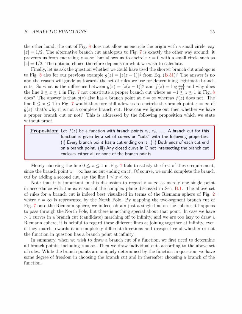
That leaves us with the question which branch cut is preferable, the single line in Fig. 8or the two-segment branch cut consisting of the line x ≤ −1 and the line x ≥ 1 analogous toFig. 7? That depends on the situation we wish to study. The former has the advantage that itallows us to encircle the point z = ∞ where f(z) = log z−1
z+1does not have a branch point. On
B ANALYTIC FUNCTIONS 25
the other hand, the cut of Fig. 8 does not allow us encircle the origin with a small circle, say|z| = 1/2. The alternative branch cut analogous to Fig. 7 is exactly the other way around: itprevents us from encircling z = ∞, but allows us to encircle z = 0 with a small circle such as|z| = 1/2. The optimal choice therefore depends on what we wish to calculate.
Finally, let us ask the question whether we could have used the shorter branch cut analogousto Fig. 8 also for our previous example g(z) = [z(z − 1)]
13 from Eq. (B.31)? The answer is no
and the reason will guide us towards the set of rules we use for determining legitimate branchcuts. So what is the difference between g(z) = [z(z − 1)]
13 and f(z) = log z−1
z+1and why does
the line 0 ≤ x ≤ 1 in Fig. 7 not constitute a proper branch cut where as −1 ≤ z ≤ 1 in Fig. 8does? The answer is that g(z) also has a branch point at z = ∞ whereas f(z) does not. Theline 0 ≤ x ≤ 1 in Fig. 7 would therefore still allow us to encircle the branch point z = ∞ ofg(z); that’s why it is not a complete branch cut. How can we figure out then whether we havea proper branch cut or not? This is addressed by the following proposition which we statewithout proof.
Proposition: Let f(z) be a function with branch points z1, z2, . . .. A branch cut for thisfunction is given by a set of curves or “cuts” with the following properties.(i) Every branch point has a cut ending on it. (ii) Both ends of each cut endon a branch point. (iii) Any closed curve in C not intersecting the branch cutencloses either all or none of the branch points.
Merely choosing the line 0 ≤ x ≤ 1 in Fig. 7 fails to satisfy the first of these requirement,since the branch point z =∞ has no cut ending on it. Of course, we could complete the branchcut by adding a second cut, say the line 1 ≤ x <∞.
Note that it is important in this discussion to regard z = ∞ as merely one single pointin accordance with the extension of the complex plane discussed in Sec. B.1. The above setof rules for a branch cut is indeed best visualized in terms of the Riemann sphere of Fig. 2where z = ∞ is represented by the North Pole. By mapping the two-segment branch cut ofFig. 7 onto the Riemann sphere, we indeed obtain just a single line on the sphere; it happensto pass through the North Pole, but there is nothing special about that point. In case we have> 1 curves in a branch cut (candidate) marching off to infinity, and we are too lazy to draw aRiemann sphere, it is helpful to regard these different lines as joining together at infinity, evenif they march towards it in completely different directions and irrespective of whether or notthe function in question has a branch point at infinity.
In summary, when we wish to draw a branch cut of a function, we first need to determineall branch points, including z = ∞. Then we draw individual cuts according to the above setof rules. While the branch points are uniquely determined by the function in question, we havesome degree of freedom in choosing the branch cut and in thereafter choosing a branch of thefunction.
B ANALYTIC FUNCTIONS 26
B.5 Mobius maps
The remainder of this section is concerned with maps between copies of the complex plane C.We start our discussion with Mobius maps.
Def. : A Mobius map M is defined as a map
M : C→ C , z 7→ w =az + b
cz + d, (B.35)
with a, b, c, d ∈ C satisfying ad 6= bc.
The condition ad− bc 6= 0 is required to have a non-trivial map. If ad = bc 6= 0, we find
d =bc
a⇒ w =
az + b
cz + d=
az + b
cz + bca
=a
c
az + b
az + b=a
c= const , (B.36)
while for a = c = 0 (a = b = 0, d = b = 0, d = c = 0) we get constants w = bd
(w = 0, w = ac,
“w =∞”).The Mobius map (B.35) is analytic except at z = −d
c. We can, however, regard it as a
map within the extended complex plane C∗ → C∗ ..= C ∪ ∞ (recall Sec. B.1). This mapM : C∗ → C∗ is bijective with inverse
M−1 : C∗ → C∗ , w 7→ z =−dw + b
cw − a , (B.37)
which is also a Mobius map. Interpreted as maps between C∗ and itself, bothM andM−1 areanalytic everywhere.
The most important property of Mobius maps is its mapping between circles and lines.
Def. : A “circline” is either a circle or a line.
Proposition: The image of a circline under a Mobius map is a circline.
Proof. The proof is based on the representation of a circline as a “circle of Apollonius”, namelythat any circline can be expressed as the set of points z ∈ C with the following property,
|z − z1| = λ|z − z2| , (B.38)
where z1 6= z2 ∈ C are reference points in the complex plane and λ ∈ R+ is a positive realnumber. In words, this expression states that a circline is made up of points with a constantdistance ratio λ to two fix points z1, z2 in the plane. The proof of this property of circlines isnot really the topic of our lectures; we therefore derive it separately in the next, nonexaminablesubsection. Note that the case λ = 1 corresponds to a line and λ 6= 1 to a circle.
B ANALYTIC FUNCTIONS 27
We will show that the image of the set of points z satisfying Eq. (B.38) under the map(B.35) results in a set of points w that also satisfies an equation of the type (B.38). Let ustherefore substitute in Eq. (B.38) for z in terms of w according to Eq. (B.37),∣∣∣∣−dw − bcw − a − z1
If cz1 + d = 0 or cz2 + d = 0, this trivially gives a circle. Otherwise,∣∣∣∣w − az1 + b
cz1 + d
∣∣∣∣ = λ
∣∣∣∣w − az2 + b
cz2 + d
∣∣∣∣ , (B.40)
and we have another circline.
Geometrically, we can determine a circline by specifying three points in C∗; a line is obtainedfor the special case where one of the points is z =∞. We obtain a similar property for Mobiusmaps.
Proposition: Let α 6= β 6= γ 6= α ∈ C∗ and α 6= β 6= γ 6= α ∈ C∗ denote 6 points inthe extended complex domain. Then there exists a Mobius map that sendsα 7→ α, β 7→ β and γ 7→ γ.
Proof. We define a first Mobius map
M1(z) =β − γβ − α
z − αz − γ , (B.41)
that maps α 7→ 0, β 7→ 1 and γ 7→ ∞. Next we define a second Mobius map
M2(z) =β − γβ − α
z − αz − γ , (B.42)
which clearly maps α 7→ 0, β 7→ 1 and γ 7→ ∞. As we have seen in Eq. (B.37), a Mobius mapis invertible, so that M−1
2 M1 is the required map. This is also a Mobius map, since Mobiusmaps form a group.
This is a convenient result; it enables us to construct for any given pair of cirlines a Mobiusmap that takes one circline to the other.
B ANALYTIC FUNCTIONS 28
A
B
C
P
d
d
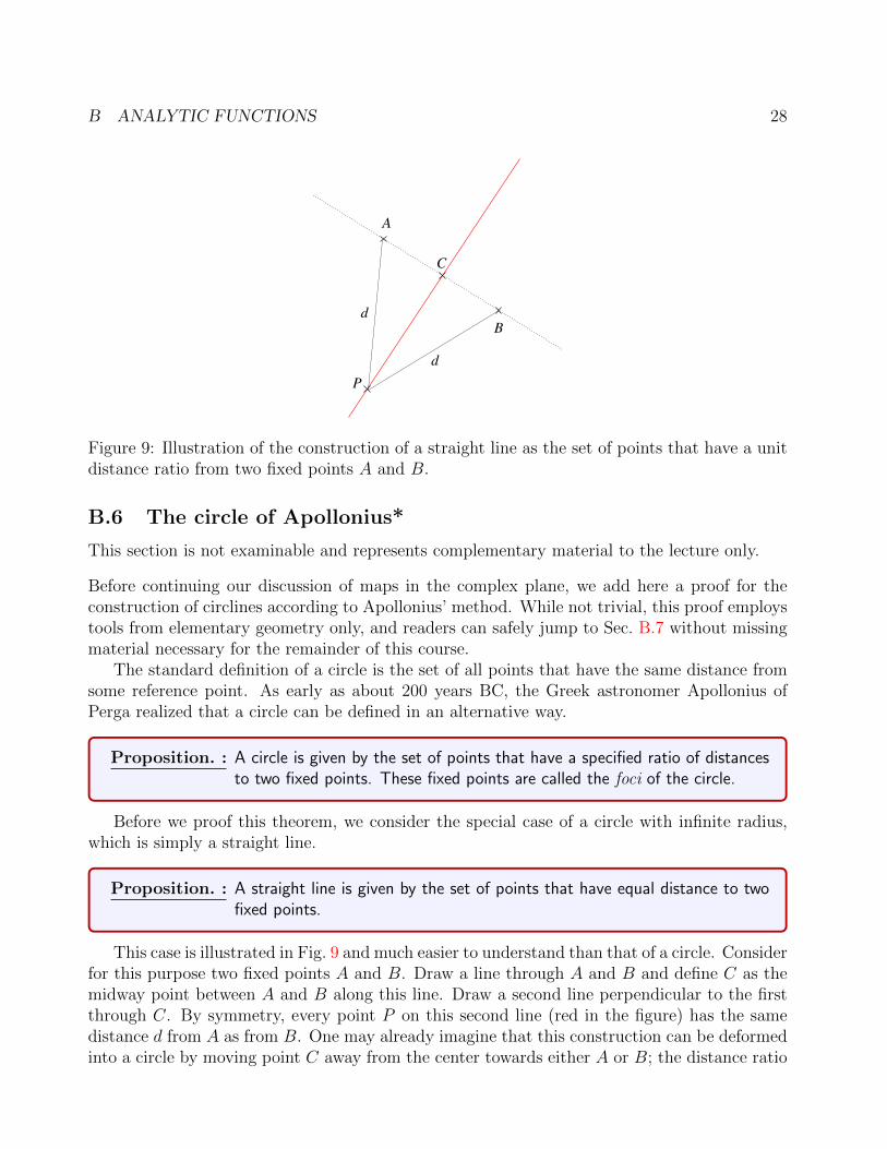
Figure 9: Illustration of the construction of a straight line as the set of points that have a unitdistance ratio from two fixed points A and B.
B.6 The circle of Apollonius*
This section is not examinable and represents complementary material to the lecture only.
Before continuing our discussion of maps in the complex plane, we add here a proof for theconstruction of circlines according to Apollonius’ method. While not trivial, this proof employstools from elementary geometry only, and readers can safely jump to Sec. B.7 without missingmaterial necessary for the remainder of this course.
The standard definition of a circle is the set of all points that have the same distance fromsome reference point. As early as about 200 years BC, the Greek astronomer Apollonius ofPerga realized that a circle can be defined in an alternative way.
Proposition. : A circle is given by the set of points that have a specified ratio of distancesto two fixed points. These fixed points are called the foci of the circle.
Before we proof this theorem, we consider the special case of a circle with infinite radius,which is simply a straight line.
Proposition. : A straight line is given by the set of points that have equal distance to twofixed points.
This case is illustrated in Fig. 9 and much easier to understand than that of a circle. Considerfor this purpose two fixed points A and B. Draw a line through A and B and define C as themidway point between A and B along this line. Draw a second line perpendicular to the firstthrough C. By symmetry, every point P on this second line (red in the figure) has the samedistance d from A as from B. One may already imagine that this construction can be deformedinto a circle by moving point C away from the center towards either A or B; the distance ratio
B ANALYTIC FUNCTIONS 29
BddλA
C
P
ssλ
E
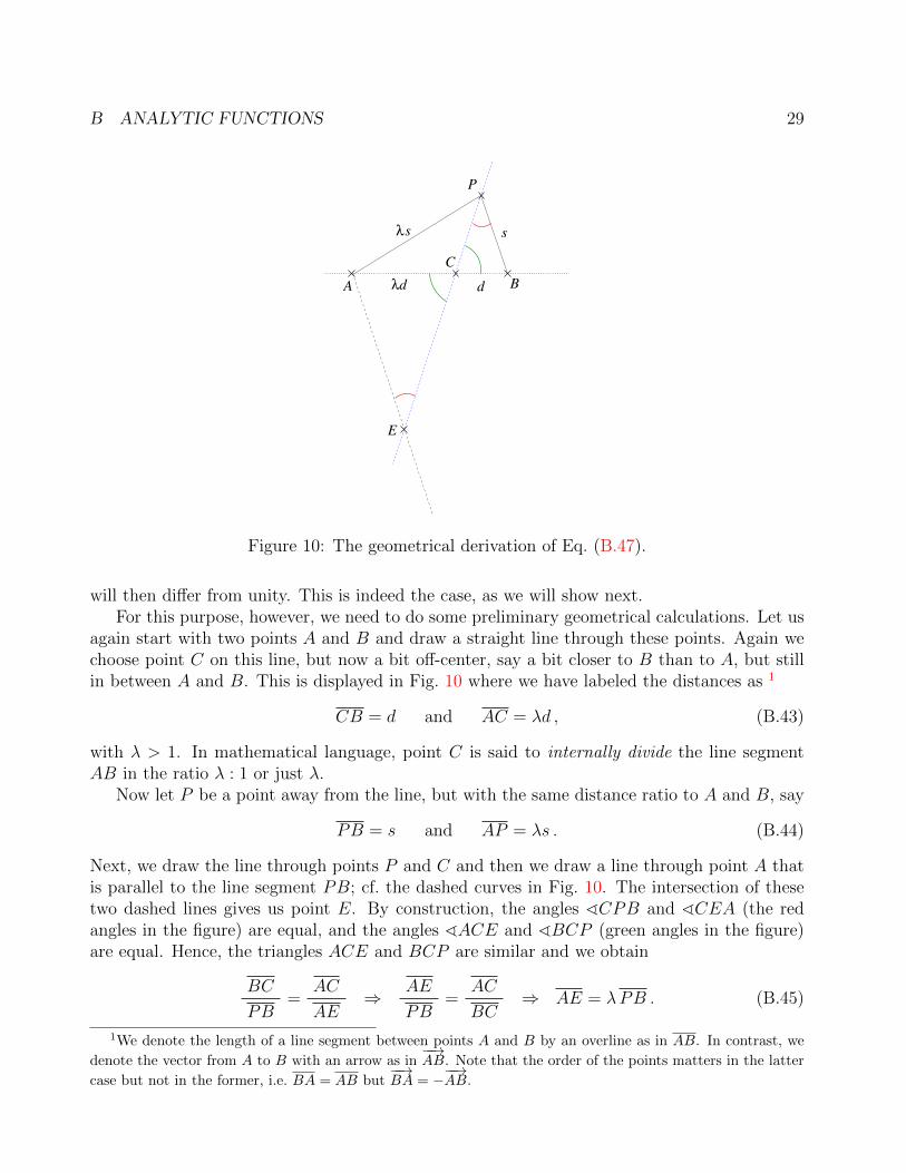
Figure 10: The geometrical derivation of Eq. (B.47).
will then differ from unity. This is indeed the case, as we will show next.For this purpose, however, we need to do some preliminary geometrical calculations. Let us
again start with two points A and B and draw a straight line through these points. Again wechoose point C on this line, but now a bit off-center, say a bit closer to B than to A, but stillin between A and B. This is displayed in Fig. 10 where we have labeled the distances as 1
CB = d and AC = λd , (B.43)
with λ > 1. In mathematical language, point C is said to internally divide the line segmentAB in the ratio λ : 1 or just λ.
Now let P be a point away from the line, but with the same distance ratio to A and B, say
PB = s and AP = λs . (B.44)
Next, we draw the line through points P and C and then we draw a line through point A thatis parallel to the line segment PB; cf. the dashed curves in Fig. 10. The intersection of thesetwo dashed lines gives us point E. By construction, the angles ^CPB and ^CEA (the redangles in the figure) are equal, and the angles ^ACE and ^BCP (green angles in the figure)are equal. Hence, the triangles ACE and BCP are similar and we obtain
BC
PB=
AC
AE⇒ AE
PB=
AC
BC⇒ AE = λPB . (B.45)
1We denote the length of a line segment between points A and B by an overline as in AB. In contrast, we
denote the vector from A to B with an arrow as in−−→AB. Note that the order of the points matters in the latter
case but not in the former, i.e. BA = AB but−−→BA = −−−→AB.
B ANALYTIC FUNCTIONS 30
BA
P
ssλ
Dd
λd
E
Figure 11: The geometrical derivation of Eq. (B.49).
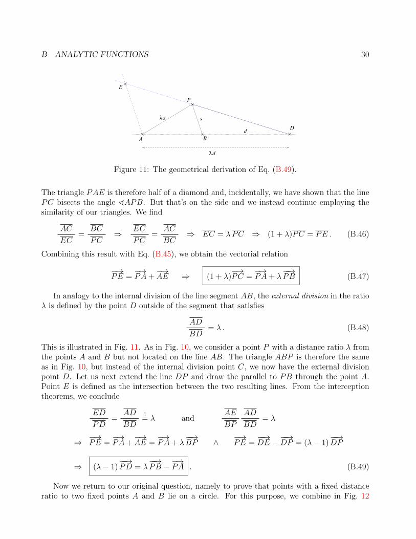
The triangle PAE is therefore half of a diamond and, incidentally, we have shown that the linePC bisects the angle ^APB. But that’s on the side and we instead continue employing thesimilarity of our triangles. We find
AC
EC=
BC
PC⇒ EC
PC=
AC
BC⇒ EC = λPC ⇒ (1 + λ)PC = PE . (B.46)
Combining this result with Eq. (B.45), we obtain the vectorial relation
−→PE =
−→PA+
−→AE ⇒ (1 + λ)
−→PC =
−→PA+ λ
−−→PB (B.47)
In analogy to the internal division of the line segment AB, the external division in the ratioλ is defined by the point D outside of the segment that satisfies
AD
BD= λ . (B.48)
This is illustrated in Fig. 11. As in Fig. 10, we consider a point P with a distance ratio λ fromthe points A and B but not located on the line AB. The triangle ABP is therefore the sameas in Fig. 10, but instead of the internal division point C, we now have the external divisionpoint D. Let us next extend the line DP and draw the parallel to PB through the point A.Point E is defined as the intersection between the two resulting lines. From the interceptiontheorems, we conclude
ED
PD=
AD
BD
!= λ and
AE
BP
AD
BD= λ
⇒ −→PE =
−→PA+
−→AE =
−→PA+ λ
−−→BP ∧ −→
PE =−−→DE −−−→DP = (λ− 1)
−−→DP
⇒ (λ− 1)−−→PD = λ
−−→PB −−→PA . (B.49)
Now we return to our original question, namely to prove that points with a fixed distanceratio to two fixed points A and B lie on a circle. For this purpose, we combine in Fig. 12
B ANALYTIC FUNCTIONS 31
BA
P
ssλ
Dd
λd
C
λd d11 2
2
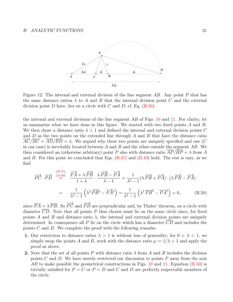
Figure 12: The internal and external division of the line segment AB. Any point P that hasthe same distance ration λ to A and B that the internal division point C and the externaldivision point D have, lies on a circle with C and D; cf. Eq. (B.50).
the internal and external divisions of the line segment AB of Figs. 10 and 11. For clarity, letus summarize what we have done in this figure. We started with two fixed points A and B.We then chose a distance ratio λ > 1 and defined the internal and external division points Cand D as the two points on the extended line through A and B that have the distance ratioAC/BC = AD/BD = λ. We argued why these two points are uniquely specified and one (Cin our case) is inevitably located between A and B and the other outside the segment AB. Wethen considered an (otherwise arbitrary) point P also with distance ratio AP/BP = λ from Aand B. For this point we concluded that Eqs. (B.47) and (B.49) hold. The rest is easy, as wefind
−→PC · −−→PD
(B.47),
(B.49)=
−→PA+ λ
−−→PB
1 + λ· λ−−→PB −−→PAλ− 1
=1
λ2 − 1(λ−−→PB +
−→PA) · (λ−−→PB −−→PA)
=1
λ2 − 1
(λ2−−→PB2 −−→PA2
)=
1
λ2 − 1
(λ2 PB
2 − PA2)
= 0 , (B.50)
since PA = λPB. So−→PC and
−−→PD are perpendicular and, by Thales’ theorem, on a circle with
diameter CD. Note that all points P thus chosen must lie on the same circle since, for fixedpoints A and B and distance ratio λ, the internal and external division points are uniquelydetermined. In consequence all P lie on the circle which has a diameter CD and includes thepoints C and D. We complete the proof with the following remarks.
1. Our restriction to distance ratios λ > 1 is without loss of generality; for 0 < λ < 1, wesimply swap the points A and B, work with the distance ratio µ ..= 1/λ > 1 and apply theproof as above.
2. Note that the set of all points P with distance ratio λ from A and B includes the divisionpoints C and D. We have merely restricted our discussion to points P away from the axisAB to make possible the geometrical constructions in Figs. 10 and 11. Equation (B.50) istrivially satisfied for P = C or P = D and C and D are perfectly respectable members ofthe circle.
B ANALYTIC FUNCTIONS 32
BA
D
C x
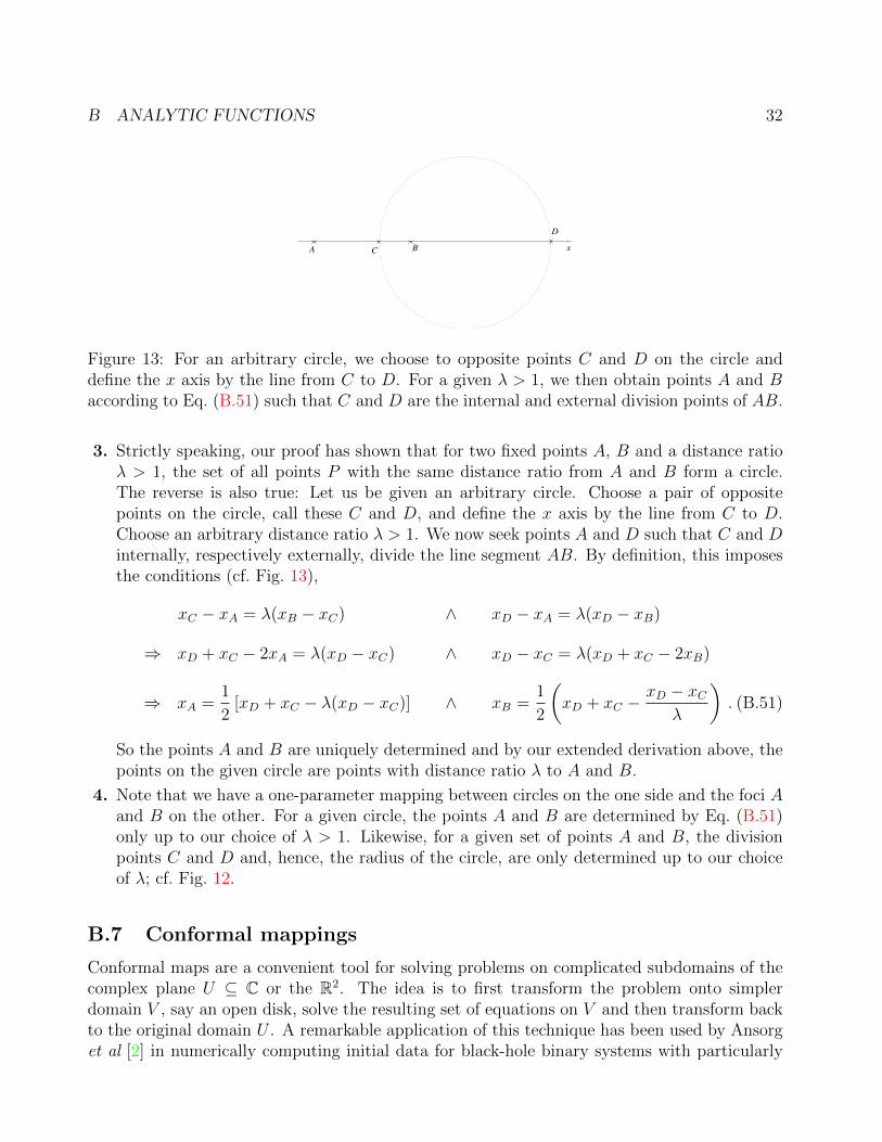
Figure 13: For an arbitrary circle, we choose to opposite points C and D on the circle anddefine the x axis by the line from C to D. For a given λ > 1, we then obtain points A and Baccording to Eq. (B.51) such that C and D are the internal and external division points of AB.
3. Strictly speaking, our proof has shown that for two fixed points A, B and a distance ratioλ > 1, the set of all points P with the same distance ratio from A and B form a circle.The reverse is also true: Let us be given an arbitrary circle. Choose a pair of oppositepoints on the circle, call these C and D, and define the x axis by the line from C to D.Choose an arbitrary distance ratio λ > 1. We now seek points A and D such that C and Dinternally, respectively externally, divide the line segment AB. By definition, this imposesthe conditions (cf. Fig. 13),
So the points A and B are uniquely determined and by our extended derivation above, thepoints on the given circle are points with distance ratio λ to A and B.
4. Note that we have a one-parameter mapping between circles on the one side and the foci Aand B on the other. For a given circle, the points A and B are determined by Eq. (B.51)only up to our choice of λ > 1. Likewise, for a given set of points A and B, the divisionpoints C and D and, hence, the radius of the circle, are only determined up to our choiceof λ; cf. Fig. 12.
B.7 Conformal mappings
Conformal maps are a convenient tool for solving problems on complicated subdomains of thecomplex plane U ⊆ C or the R2. The idea is to first transform the problem onto simplerdomain V , say an open disk, solve the resulting set of equations on V and then transform backto the original domain U . A remarkable application of this technique has been used by Ansorget al [2] in numerically computing initial data for black-hole binary systems with particularly
B ANALYTIC FUNCTIONS 33
θ
2θ
r
r2
r
r2
θ
2θ x
y
x
θ
r
θ
r
r
θ/2θ/2
r
y
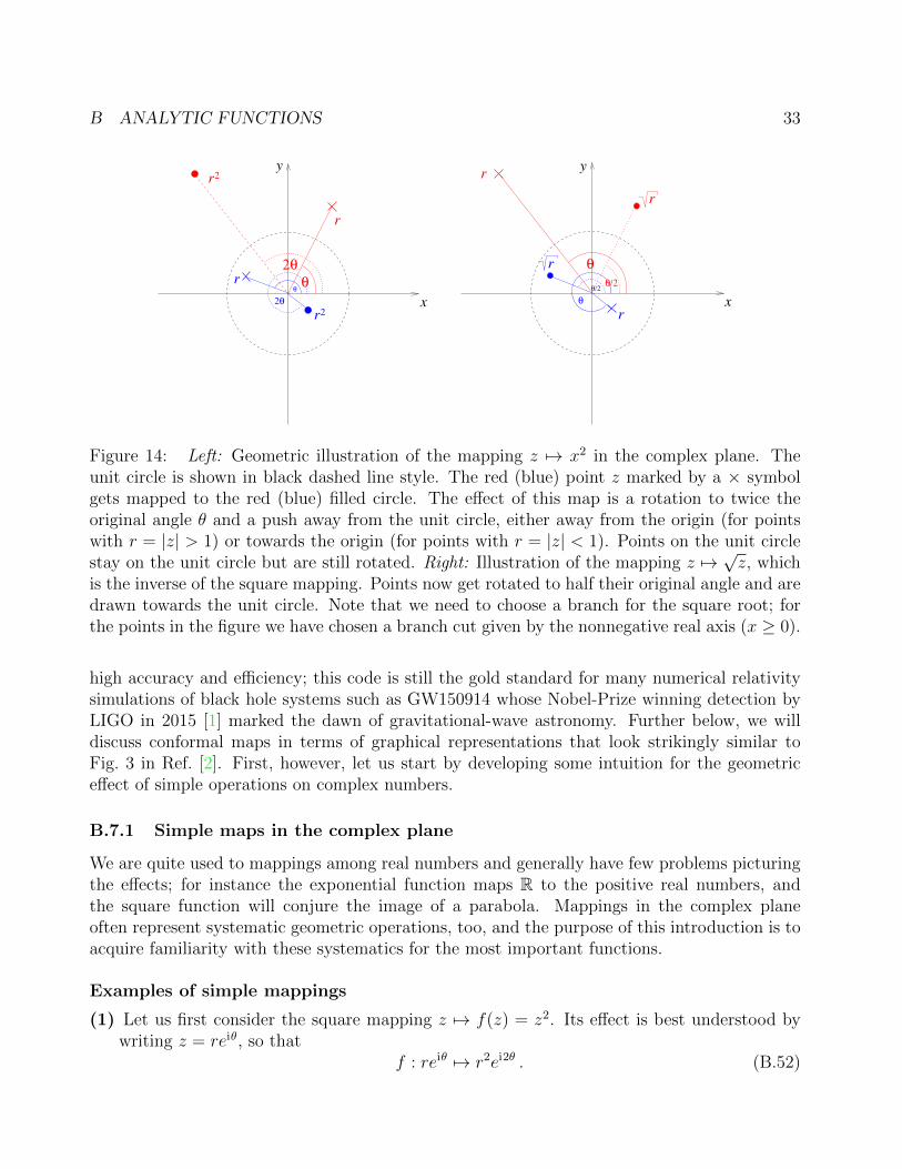
Figure 14: Left: Geometric illustration of the mapping z 7→ x2 in the complex plane. Theunit circle is shown in black dashed line style. The red (blue) point z marked by a × symbolgets mapped to the red (blue) filled circle. The effect of this map is a rotation to twice theoriginal angle θ and a push away from the unit circle, either away from the origin (for pointswith r = |z| > 1) or towards the origin (for points with r = |z| < 1). Points on the unit circlestay on the unit circle but are still rotated. Right: Illustration of the mapping z 7→ √z, whichis the inverse of the square mapping. Points now get rotated to half their original angle and aredrawn towards the unit circle. Note that we need to choose a branch for the square root; forthe points in the figure we have chosen a branch cut given by the nonnegative real axis (x ≥ 0).
high accuracy and efficiency; this code is still the gold standard for many numerical relativitysimulations of black hole systems such as GW150914 whose Nobel-Prize winning detection byLIGO in 2015 [1] marked the dawn of gravitational-wave astronomy. Further below, we willdiscuss conformal maps in terms of graphical representations that look strikingly similar toFig. 3 in Ref. [2]. First, however, let us start by developing some intuition for the geometriceffect of simple operations on complex numbers.
B.7.1 Simple maps in the complex plane
We are quite used to mappings among real numbers and generally have few problems picturingthe effects; for instance the exponential function maps R to the positive real numbers, andthe square function will conjure the image of a parabola. Mappings in the complex planeoften represent systematic geometric operations, too, and the purpose of this introduction is toacquire familiarity with these systematics for the most important functions.
Examples of simple mappings
(1) Let us first consider the square mapping z 7→ f(z) = z2. Its effect is best understood bywriting z = reiθ, so that
f : reiθ 7→ r2ei2θ . (B.52)
B ANALYTIC FUNCTIONS 34
x1
π
y
−π
x+iy0
yθ=
r=ex
0
x1
π
y
−π
x +iy0
r=e x0
θ= y
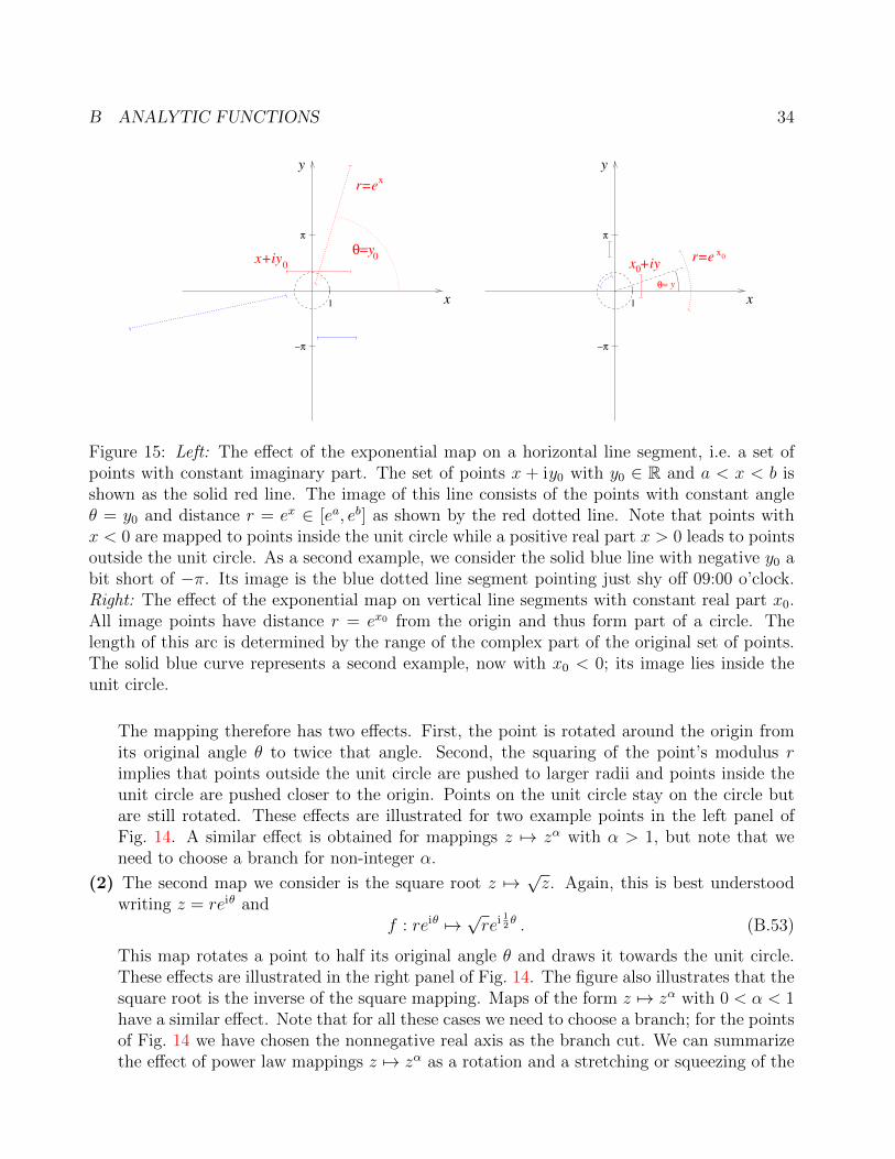
Figure 15: Left: The effect of the exponential map on a horizontal line segment, i.e. a set ofpoints with constant imaginary part. The set of points x + iy0 with y0 ∈ R and a < x < b isshown as the solid red line. The image of this line consists of the points with constant angleθ = y0 and distance r = ex ∈ [ea, eb] as shown by the red dotted line. Note that points withx < 0 are mapped to points inside the unit circle while a positive real part x > 0 leads to pointsoutside the unit circle. As a second example, we consider the solid blue line with negative y0 abit short of −π. Its image is the blue dotted line segment pointing just shy off 09:00 o’clock.Right: The effect of the exponential map on vertical line segments with constant real part x0.All image points have distance r = ex0 from the origin and thus form part of a circle. Thelength of this arc is determined by the range of the complex part of the original set of points.The solid blue curve represents a second example, now with x0 < 0; its image lies inside theunit circle.
The mapping therefore has two effects. First, the point is rotated around the origin fromits original angle θ to twice that angle. Second, the squaring of the point’s modulus rimplies that points outside the unit circle are pushed to larger radii and points inside theunit circle are pushed closer to the origin. Points on the unit circle stay on the circle butare still rotated. These effects are illustrated for two example points in the left panel ofFig. 14. A similar effect is obtained for mappings z 7→ zα with α > 1, but note that weneed to choose a branch for non-integer α.
(2) The second map we consider is the square root z 7→ √z. Again, this is best understoodwriting z = reiθ and
f : reiθ 7→ √rei 12θ . (B.53)
This map rotates a point to half its original angle θ and draws it towards the unit circle.These effects are illustrated in the right panel of Fig. 14. The figure also illustrates that thesquare root is the inverse of the square mapping. Maps of the form z 7→ zα with 0 < α < 1have a similar effect. Note that for all these cases we need to choose a branch; for the pointsof Fig. 14 we have chosen the nonnegative real axis as the branch cut. We can summarizethe effect of power law mappings z 7→ zα as a rotation and a stretching or squeezing of the
B ANALYTIC FUNCTIONS 35
original point’s distance from the origin.
(3) The exponential map is best understood by writing z = x+ iy, whence
f : (x+ iy) 7→ ex+iy = reiy with r = ex . (B.54)
The real part of the input number thus determines the distance r of the image pointfrom the origin and the imaginary part determines the argument or angle of the image.It is instructive to consider the images of horizontal or vertical line segments under theexponential map as illustrated in Fig. 15. Horizontal lines with constant imaginary party0 and real range c ≤ x ≤ d are mapped to points with constant angle θ = y0 and formpart of a radial ray with extent ea ≤ r ≤ eb. A vertical line, in contrast, has constant realpart and is therefore mapped to a segment of a circle of radius r = ex0 with the angularrange determined by the imaginary extent of the original line. Note that vertical curvesto the right of the y axis with x0 > 0 result in images outside the unit sphere and thoseto the left of the y axis are mapped inside the unit circle; cf. the red and blue curves inthe right panel of Fig. 15. A Rectangle is bounded by two vertical and two horizontal linesegments, which are mapped to two circle segments and two ray segments, respectively.The exponential function thus maps rectangles to sectors of annuli (“annulus” is Latin for“ring” which I remember best by recalling the Spanish title of J.R.R. Tolkien’s epic “Elsenor de los anillos”).
(4) The logarithmic map z 7→ ln z is the inverse operation of the exponential mapping, providedwe have appropriately chosen a branch. It therefore maps sectors of annuli to rectangles.
B.7.2 Conformal maps
Having established the effects of simple maps, we turn our attention to the specific class ofconformal maps.
Def. : A conformal map is a map f : U → V between open subsets U, V of C whichis analytic and whose derivative f ′ is non-zero throughout U . In practice, we oftenrequire this map to be bijective; this requirement is sometimes made explicit by callingthe map a conformal equivalence.
One can alternatively define a conformal map in terms of its action on the angle betweenintersecting curves.
Proposition: A conformal map preserves the angle in magnitude and orientation betweenintersecting curves.
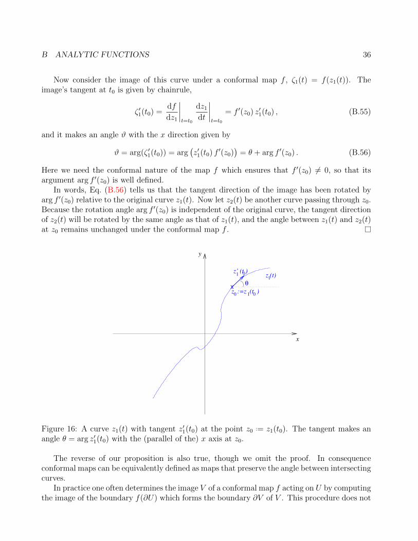
Proof. Let z1(t) be a curve in C, parametrized by t ∈ R, that passes through a point z0..= z(t0)
with nonzero derivative z′1(t0). The curve then makes an angle θ = arg z′1(t0) relative to the xdirection at z0; cf. Fig. 16.
B ANALYTIC FUNCTIONS 36
Now consider the image of this curve under a conformal map f , ζ1(t) = f(z1(t)). Theimage’s tangent at t0 is given by chainrule,
ζ ′1(t0) =df
dz1
∣∣∣∣t=t0
dz1
dt
∣∣∣∣t=t0
= f ′(z0) z′1(t0) , (B.55)
and it makes an angle ϑ with the x direction given by
ϑ = arg(ζ ′1(t0)) = arg(z′1(t0) f ′(z0)
)= θ + arg f ′(z0) . (B.56)
Here we need the conformal nature of the map f which ensures that f ′(z0) 6= 0, so that itsargument arg f ′(z0) is well defined.
In words, Eq. (B.56) tells us that the tangent direction of the image has been rotated byarg f ′(z0) relative to the original curve z1(t). Now let z2(t) be another curve passing through z0.Because the rotation angle arg f ′(z0) is independent of the original curve, the tangent directionof z2(t) will be rotated by the same angle as that of z1(t), and the angle between z1(t) and z2(t)at z0 remains unchanged under the conformal map f .
x
y
z (t)
x
1
θ
0 0z :=z (t )
1
z’ (t )01
Figure 16: A curve z1(t) with tangent z′1(t0) at the point z0..= z1(t0). The tangent makes an
angle θ = arg z′1(t0) with the (parallel of the) x axis at z0.
The reverse of our proposition is also true, though we omit the proof. In consequenceconformal maps can be equivalently defined as maps that preserve the angle between intersectingcurves.
In practice one often determines the image V of a conformal map f acting on U by computingthe image of the boundary f(∂U) which forms the boundary ∂V of V . This procedure does not
B ANALYTIC FUNCTIONS 37
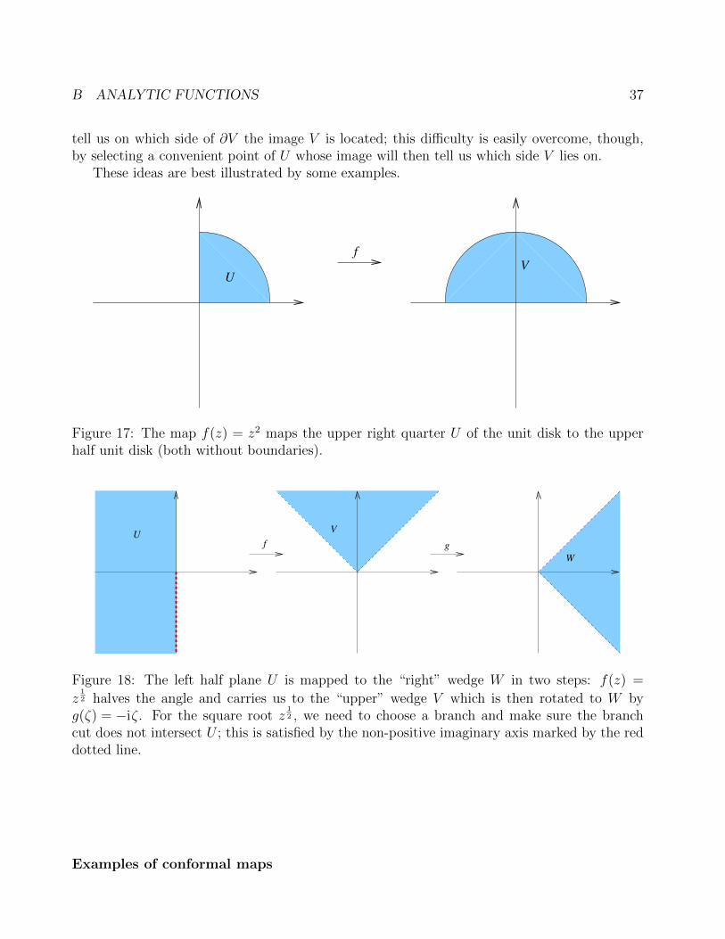
tell us on which side of ∂V the image V is located; this difficulty is easily overcome, though,by selecting a convenient point of U whose image will then tell us which side V lies on.
These ideas are best illustrated by some examples.
UV
f
Figure 17: The map f(z) = z2 maps the upper right quarter U of the unit disk to the upperhalf unit disk (both without boundaries).
Uf g
V
W
Figure 18: The left half plane U is mapped to the “right” wedge W in two steps: f(z) =
z12 halves the angle and carries us to the “upper” wedge V which is then rotated to W byg(ζ) = −iζ. For the square root z
12 , we need to choose a branch and make sure the branch
cut does not intersect U ; this is satisfied by the non-positive imaginary axis marked by the reddotted line.
Examples of conformal maps
B ANALYTIC FUNCTIONS 38
(1) The map f(z) = az + b with a, b ∈ C and a 6= 0 is clearly analytic everywhere withnon-zero derivative f ′(z) = a and hence conformal. It rotates points by arg a, enlargesor reduces their distance from the origin by a factor |a| and translates by b.
(2) The function f(z) = z2 is analytic everywhere, but its derivative vanishes at z = 0, soit is a conformal map as long as we exclude the origin. For example, it is a conformalmap from the upper right quadrant of the unit disk,
U =z ∈ C
∣∣∣ 0 < |z| < 1 ∧ 0 < arg z <π
2
to the upper half disk
V =w ∈ C
∣∣∣ 0 < |w| < 1 ∧ 0 < argw < π,
as illustrated in Fig. 17. Note that the three boundary segments of U form right anglesat the points z = 0, z = 1 and z = i. The latter two points are mapped to w = 1,w = −1 where the boundary segments of V also form right angles, as they should sinceconformal maps preserve angles. The right angle at z = 0, however, is not preservedat w = 0; this is not surprising, since the map f is not conformal at z = 0.
(3) Often, one is looking for a conformal map that transforms between two given subsetsof the complex plane. Let us determine, for example, which conformal map carries usfrom the left half plane
U =z ∈ C
∣∣∣ Re(z) < 0
to the “right” wedge
W =w ∈ C
∣∣∣ − π
4< argw <
π
4
.
From the graphical illustration of U and W in Fig. 18, we see that we need to halfthe angular range. This is achieved by taking the square root f(z) = z1/2, but for thisfunction with non-integer exponent we need to choose an appropriate branch. Becausewe require f(z) to be analytic on U , the branch cut must not intersect U which excludesthe principal branch arg z ∈ (−π, π]. Instead, we can put the branch cut on the non-positive imaginary axis as shown by the red dotted line in the figure and choose, forexample, arg z ∈
(−π
2, 3π
2
]. Under the mapping f , however, this gives us the “upper”
wedge V displayed in the middle of Fig. 18. We need a rotation by −π/2 to arriveat our destination W , which is achieved by multiplication with e−iπ/2 = −i, i.e. anadditional map g(ζ) = −iζ. The complete map from U to W is then
g f(z) = −iz12 .
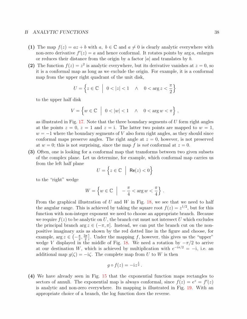
(4) We have already seen in Fig. 15 that the exponential function maps rectangles tosectors of annuli. The exponential map is always conformal, since f(z) = ez = f ′(z)is analytic and non-zero everywhere. Its mapping is illustrated in Fig. 19. With anappropriate choice of a branch, the log function does the reverse.
B ANALYTIC FUNCTIONS 39
f
e xe
x1 2
y1
y2
V
x x
y
y
i
i
1 2
2
1
U
Figure 19: The exponential map f(z) = ez takes rectangles to sectors of annuli. With appro-priate choice of branch, the log function does the inverse operation.
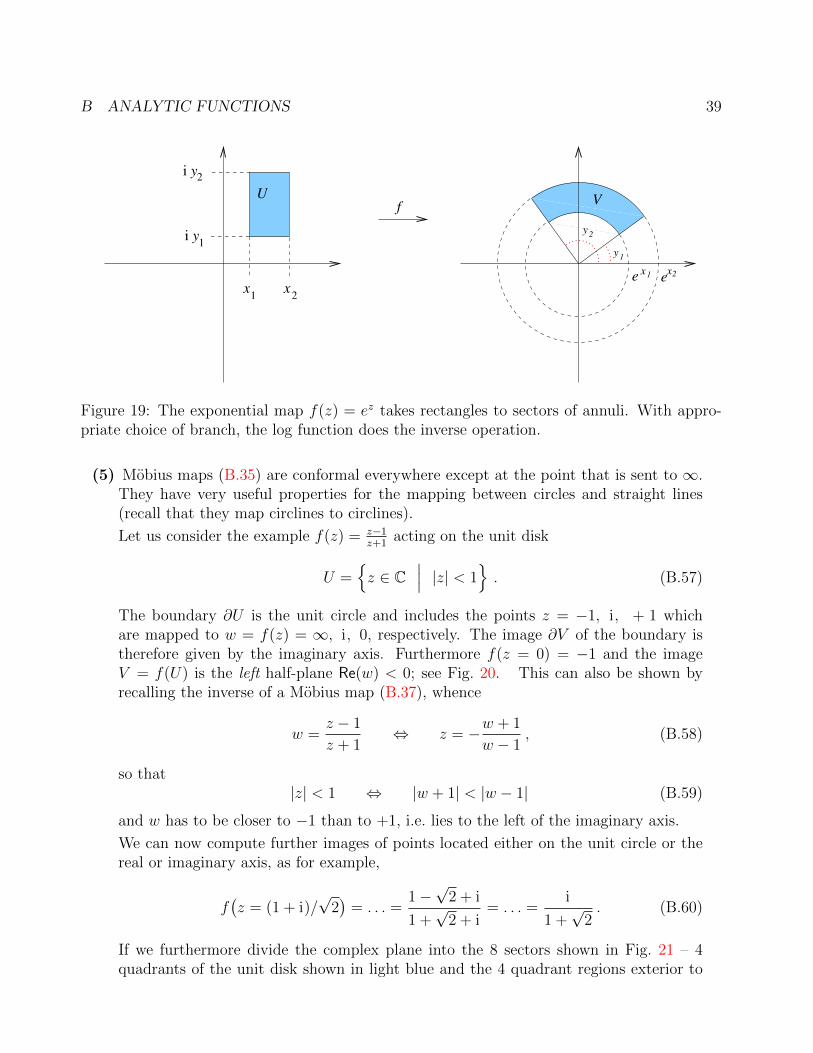
(5) Mobius maps (B.35) are conformal everywhere except at the point that is sent to ∞.They have very useful properties for the mapping between circles and straight lines(recall that they map circlines to circlines).
Let us consider the example f(z) = z−1z+1
acting on the unit disk
U =z ∈ C
∣∣∣ |z| < 1. (B.57)
The boundary ∂U is the unit circle and includes the points z = −1, i, + 1 whichare mapped to w = f(z) = ∞, i, 0, respectively. The image ∂V of the boundary istherefore given by the imaginary axis. Furthermore f(z = 0) = −1 and the imageV = f(U) is the left half-plane Re(w) < 0; see Fig. 20. This can also be shown byrecalling the inverse of a Mobius map (B.37), whence
w =z − 1
z + 1⇔ z = −w + 1
w − 1, (B.58)
so that|z| < 1 ⇔ |w + 1| < |w − 1| (B.59)
and w has to be closer to −1 than to +1, i.e. lies to the left of the imaginary axis.
We can now compute further images of points located either on the unit circle or thereal or imaginary axis, as for example,
f(z = (1 + i)/
√2)
= . . . =1−√
2 + i
1 +√
2 + i= . . . =
i
1 +√
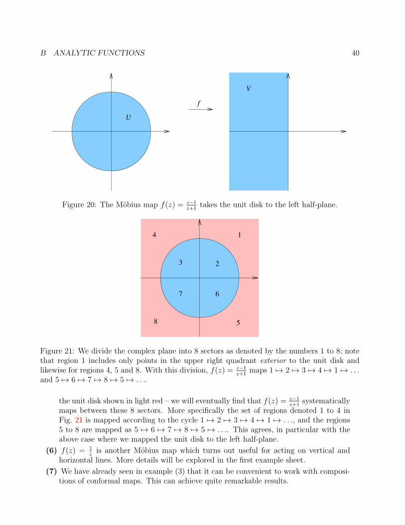
2. (B.60)
If we furthermore divide the complex plane into the 8 sectors shown in Fig. 21 – 4quadrants of the unit disk shown in light blue and the 4 quadrant regions exterior to
B ANALYTIC FUNCTIONS 40
U
f
V
Figure 20: The Mobius map f(z) = z−1z+1
takes the unit disk to the left half-plane.
1
23
4
5
67
8
Figure 21: We divide the complex plane into 8 sectors as denoted by the numbers 1 to 8; notethat region 1 includes only points in the upper right quadrant exterior to the unit disk andlikewise for regions 4, 5 and 8. With this division, f(z) = z−1
z+1maps 1 7→ 2 7→ 3 7→ 4 7→ 1 7→ . . .
and 5 7→ 6 7→ 7 7→ 8 7→ 5 7→ . . ..
the unit disk shown in light red – we will eventually find that f(z) = z−1z+1
systematicallymaps between these 8 sectors. More specifically the set of regions denoted 1 to 4 inFig. 21 is mapped according to the cycle 1 7→ 2 7→ 3 7→ 4 7→ 1 7→ . . ., and the regions5 to 8 are mapped as 5 7→ 6 7→ 7 7→ 8 7→ 5 7→ . . .. This agrees, in particular with theabove case where we mapped the unit disk to the left half-plane.
(6) f(z) = 1z
is another Mobius map which turns out useful for acting on vertical andhorizontal lines. More details will be explored in the first example sheet.
(7) We have already seen in example (3) that it can be convenient to work with composi-tions of conformal maps. This can achieve quite remarkable results.
B ANALYTIC FUNCTIONS 41
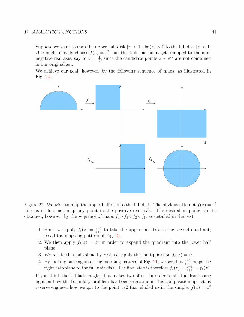
Suppose we want to map the upper half disk |z| < 1 , Im(z) > 0 to the full disc |z| < 1.One might naively choose f(z) = z2, but this fails: no point gets mapped to the non-negative real axis, say to w = 1
2, since the candidate points z ∼ eiπ are not contained
in our original set.
We achieve our goal, however, by the following sequence of maps, as illustrated inFig. 22.
W
ff1 2
f3
f4
Figure 22: We wish to map the upper half disk to the full disk. The obvious attempt f(z) = z2
fails as it does not map any point to the positive real axis. The desired mapping can beobtained, however, by the sequence of maps f4 f3 f2 f1, as detailed in the text.
1. First, we apply f1(z) = z−1z+1
to take the upper half-disk to the second quadrant;recall the mapping pattern of Fig. 21.
2. We then apply f2(z) = z2 in order to expand the quadrant into the lower halfplane.
3. We rotate this half-plane by π/2, i.e. apply the multiplication f3(z) = iz.
4. By looking once again at the mapping pattern of Fig. 21, we see that z−1z+1
maps the
right half-plane to the full unit disk. The final step is therefore f4(z) = z−1z+1
= f1(z).
If you think that’s black magic, that makes two of us. In order to shed at least somelight on how the boundary problem has been overcome in this composite map, let usreverse engineer how we got to the point 1/2 that eluded us in the simpler f(z) = z2
B ANALYTIC FUNCTIONS 42
attempt. The last three steps towards 1/2 are rather easily inverted,
f−14 (1
2) = 3 , f−1
3 (3) = −3i = 3e−i3π/2 , f−12 (−3i) =
√3e−i3π/4 . (B.61)
We could plug the final value into f−11 , but that would be more work and not necessary;
the key point is that√
3e−i3π/4 is located somewhere in the interior of region 4 inFig. 21; in particular, it is not located on the boundary of that region and thereforehas to originate somewhere in the interior of region 3.
B.7.3 Laplace’s equation and conformal maps
We have seen in Sec. B.3 that the real and imaginary parts of an analytic function are harmonicand solutions to the Laplace equation. By chain rule, the composition of an analytic functionand a conformal map is also analytic, so that its real and imaginary part are also harmonic. Onecan therefore use conformal maps to carry solutions of Laplace’s equation in some (convenientlychosen “simple”) domain to a solution of Laplace’s equation in another (more complicated)domain.
For this purpose, we will identify the complex domain C with R2 according to z ↔ x+ iy.Let U ⊆ R2 be some “tricky” domain and f : U → V a conformal map to a much nicer domainV as illustrated in Fig. 23. Our goal is to find a solution φ(x, y) of the Laplace equation
4φ = ∂2xφ+ ∂2
yφ = 0 (B.62)
in U subject to some Dirichlet boundary conditions on ∂U . This can be achieved as follows.
1. The conformal map f carries points from U to points in V according to
f : U → V , z = x+ iy 7→ ζ = u+ iv . (B.63)
2. The Dirichlet boundary conditions φ(x, y) = φ0(x, y) on ∂U translate into boundary con-ditions Φ(u, v) = Φ0(u, v) on ∂V .
3. Now we solve the Laplace equation4Φ = 0 on the nice domain V subject to the boundaryconditions on ∂V .
4. Then the solution on U is given by
φ(x, y) = Φ(Re(f(x+ iy)), Im(f(x+ iy))
). (B.64)
The final expression looks more complicated than it really is, and we can write it in muchsimpler from if we (formally incorrectly) set “z = (x, y)” and “ζ = (u, v)”. This improperversion of Eq. (B.64) becomes “φ(z) = Φ
(f(z)
)”.
The proof of Eq. (B.64) is remarkably simple given the knowledge we already have. As wehave seen in Sec. B.3, a solution Φ(u, v) to the Laplace equation is harmonic and, hence, thereal part of an analytic complex function G(ζ). The conformal map f is analytic by definition,so that g = G f is a complex analytic function on U . Finally g(z) = G(f(z)), so that the real
B ANALYTIC FUNCTIONS 43
U
x
f
x
V
G
g
x
z = x+ iy ζ = f(z) = u+ iv
= G f(z) = G(ζ) = Φ(u, v) + iΨ(u, v)
g(z) = φ(x, y) + iψ(x, y)
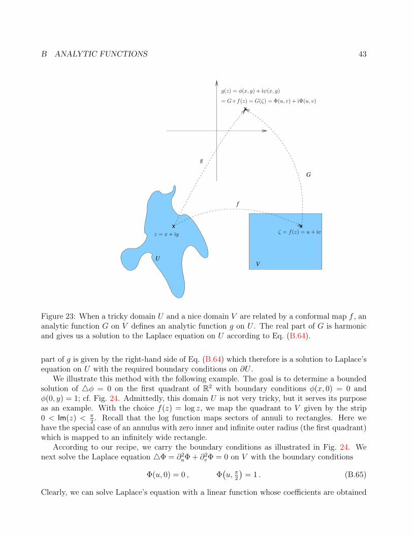
Figure 23: When a tricky domain U and a nice domain V are related by a conformal map f , ananalytic function G on V defines an analytic function g on U . The real part of G is harmonicand gives us a solution to the Laplace equation on U according to Eq. (B.64).
part of g is given by the right-hand side of Eq. (B.64) which therefore is a solution to Laplace’sequation on U with the required boundary conditions on ∂U .
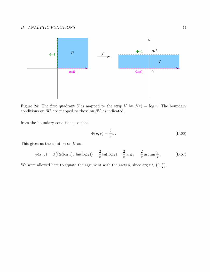
We illustrate this method with the following example. The goal is to determine a boundedsolution of 4φ = 0 on the first quadrant of R2 with boundary conditions φ(x, 0) = 0 andφ(0, y) = 1; cf. Fig. 24. Admittedly, this domain U is not very tricky, but it serves its purposeas an example. With the choice f(z) = log z, we map the quadrant to V given by the strip0 < Im(z) < π
2. Recall that the log function maps sectors of annuli to rectangles. Here we
have the special case of an annulus with zero inner and infinite outer radius (the first quadrant)which is mapped to an infinitely wide rectangle.
According to our recipe, we carry the boundary conditions as illustrated in Fig. 24. Wenext solve the Laplace equation 4Φ = ∂2
uΦ + ∂2vΦ = 0 on V with the boundary conditions
Φ(u, 0) = 0 , Φ(u, π
2
)= 1 . (B.65)
Clearly, we can solve Laplace’s equation with a linear function whose coefficients are obtained
B ANALYTIC FUNCTIONS 44
f
V
Uπ/2
0
φ=1
φ=0
Φ=1
Φ=0
Figure 24: The first quadrant U is mapped to the strip V by f(z) = log z. The boundaryconditions on ∂U are mapped to those on ∂V as indicated.
from the boundary conditions, so that
Φ(u, v) =2
πv . (B.66)
This gives us the solution on U as
φ(x, y) = Φ(Re(log z), Im(log z)
)=
2
πIm(log z) =
2
πarg z =
2
πarctan
y
x. (B.67)
We were allowed here to equate the argument with the arctan, since arg z ∈(0, π
2
).
C CONTOUR INTEGRATION AND CAUCHY’S THEOREM 45
C Contour Integration and Cauchy’s theorem
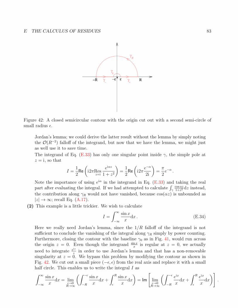
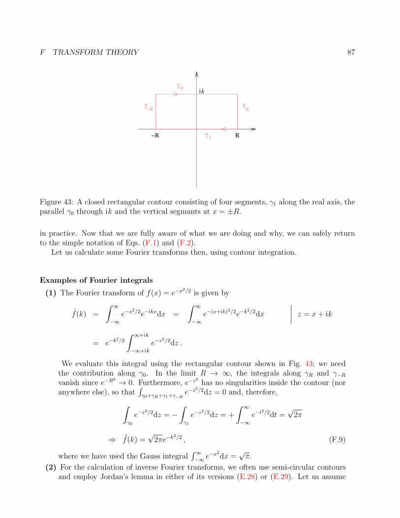
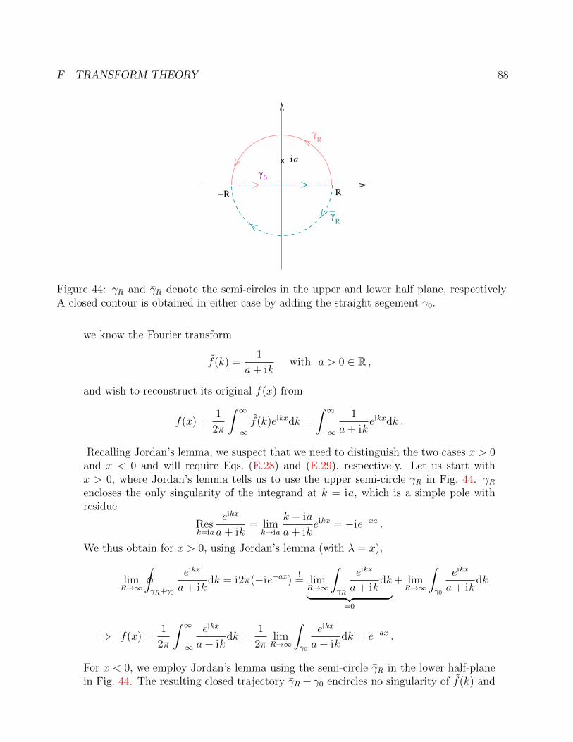
The remainder of these notes will focus on the integration of complex functions. We havealready seen that the differentiation of complex functions reveals some remarkable featuresquite different from those known for real functions. This will be even more pronounced in thecase of integration. In fact, complex integration will allow us to compute some very tricky realintegrals by pretending they were complex.
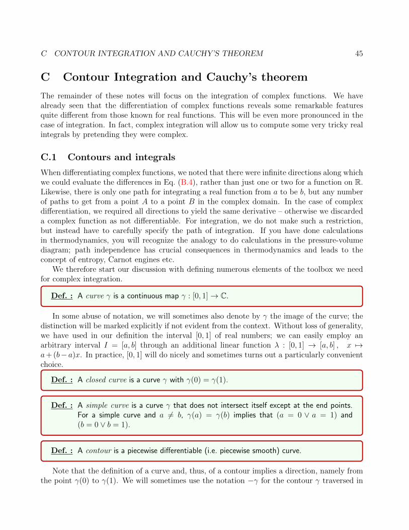
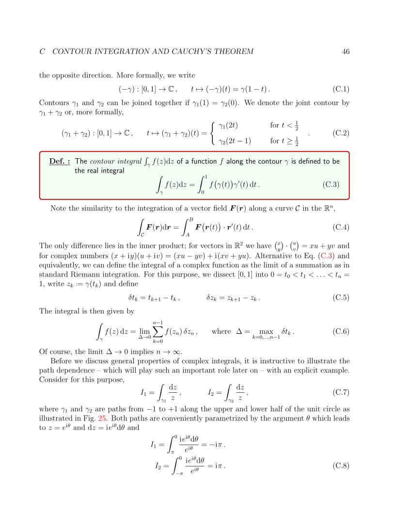
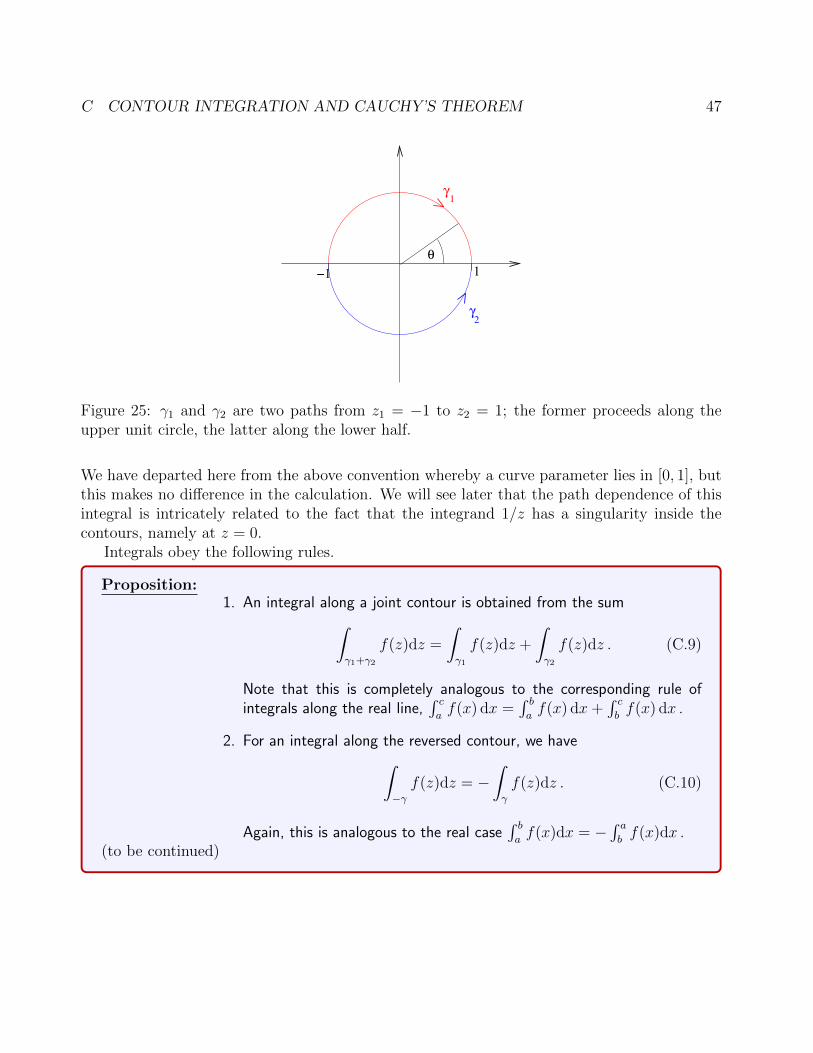
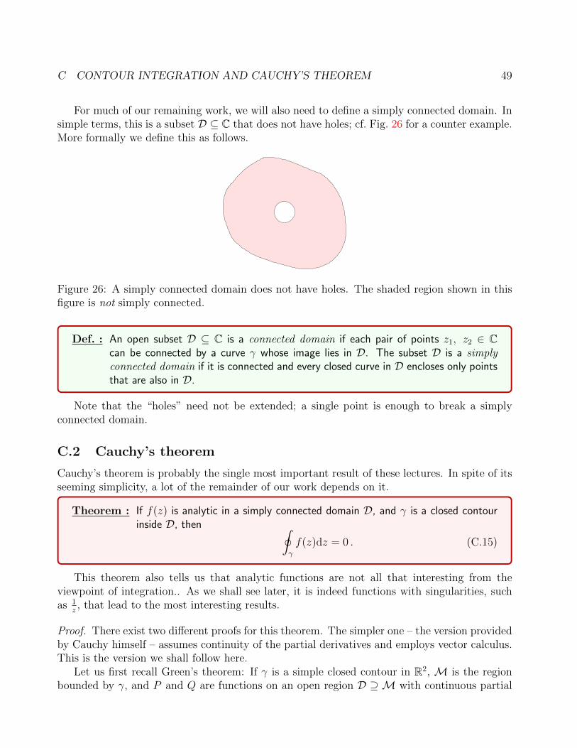
C.1 Contours and integrals
When differentiating complex functions, we noted that there were infinite directions along whichwe could evaluate the differences in Eq. (B.4), rather than just one or two for a function on R.Likewise, there is only one path for integrating a real function from a to be b, but any numberof paths to get from a point A to a point B in the complex domain. In the case of complexdifferentiation, we required all directions to yield the same derivative – otherwise we discardeda complex function as not differentiable. For integration, we do not make such a restriction,but instead have to carefully specify the path of integration. If you have done calculationsin thermodynamics, you will recognize the analogy to do calculations in the pressure-volumediagram; path independence has crucial consequences in thermodynamics and leads to theconcept of entropy, Carnot engines etc.
We therefore start our discussion with defining numerous elements of the toolbox we needfor complex integration.
Def. : A curve γ is a continuous map γ : [0, 1]→ C.
In some abuse of notation, we will sometimes also denote by γ the image of the curve; thedistinction will be marked explicitly if not evident from the context. Without loss of generality,we have used in our definition the interval [0, 1] of real numbers; we can easily employ anarbitrary interval I = [a, b] through an additional linear function λ : [0, 1] → [a, b] , x 7→a+ (b− a)x. In practice, [0, 1] will do nicely and sometimes turns out a particularly convenientchoice.
Def. : A closed curve is a curve γ with γ(0) = γ(1).
Def. : A simple curve is a curve γ that does not intersect itself except at the end points.For a simple curve and a 6= b, γ(a) = γ(b) implies that (a = 0 ∨ a = 1) and(b = 0 ∨ b = 1).
Def. : A contour is a piecewise differentiable (i.e. piecewise smooth) curve.
Note that the definition of a curve and, thus, of a contour implies a direction, namely fromthe point γ(0) to γ(1). We will sometimes use the notation −γ for the contour γ traversed in
C CONTOUR INTEGRATION AND CAUCHY’S THEOREM 46
the opposite direction. More formally, we write
(−γ) : [0, 1]→ C , t 7→ (−γ)(t) = γ(1− t) . (C.1)
Contours γ1 and γ2 can be joined together if γ1(1) = γ2(0). We denote the joint contour byγ1 + γ2 or, more formally,
(γ1 + γ2) : [0, 1]→ C , t 7→ (γ1 + γ2)(t) =
γ1(2t) for t < 1
2
γ2(2t− 1) for t ≥ 12
. (C.2)
Def. : The contour integral∫γf(z)dz of a function f along the contour γ is defined to be
the real integral ∫γ
f(z)dz =
∫ 1
0
f(γ(t)
)γ′(t) dt . (C.3)
Note the similarity to the integration of a vector field F (r) along a curve C in the Rn,∫CF (r)dr =
∫ B
A
F(r(t)
)· r′(t) dt . (C.4)
The only difference lies in the inner product; for vectors in R2 we have(xy
)·(uv
)= xu+ yv and
for complex numbers (x + iy)(u + iv) = (xu− yv) + i(xv + yu). Alternative to Eq. (C.3) andequivalently, we can define the integral of a complex function as the limit of a summation as instandard Riemann integration. For this purpose, we dissect [0, 1] into 0 = t0 < t1 < . . . < tn =1, write zk ..= γ(tk) and define
δtk = tk+1 − tk , δzk = zk+1 − zk . (C.5)
The integral is then given by∫γ
f(z) dz = lim∆→0
n−1∑k=0
f(zn) δzn , where ∆ = maxk=0,...,n−1
δtk . (C.6)
Of course, the limit ∆→ 0 implies n→∞.Before we discuss general properties of complex integrals, it is instructive to illustrate the
path dependence – which will play such an important role later on – with an explicit example.Consider for this purpose,
I1 =
∫γ1
dz
z, I2 =
∫γ2
dz
z, (C.7)
where γ1 and γ2 are paths from −1 to +1 along the upper and lower half of the unit circle asillustrated in Fig. 25. Both paths are conveniently parametrized by the argument θ which leadsto z = eiθ and dz = ieiθdθ and
I1 =
∫ 0
π
ieiθdθ
eiθ= −iπ .
I2 =
∫ 0
−π
ieiθdθ
eiθ= iπ . (C.8)
C CONTOUR INTEGRATION AND CAUCHY’S THEOREM 47
θ
γ
γ1
2
1−1
Figure 25: γ1 and γ2 are two paths from z1 = −1 to z2 = 1; the former proceeds along theupper unit circle, the latter along the lower half.
We have departed here from the above convention whereby a curve parameter lies in [0, 1], butthis makes no difference in the calculation. We will see later that the path dependence of thisintegral is intricately related to the fact that the integrand 1/z has a singularity inside thecontours, namely at z = 0.
Integrals obey the following rules.
Proposition:1. An integral along a joint contour is obtained from the sum∫
γ1+γ2
f(z)dz =
∫γ1
f(z)dz +
∫γ2
f(z)dz . (C.9)
Note that this is completely analogous to the corresponding rule ofintegrals along the real line,
∫ caf(x) dx =
∫ baf(x) dx+
∫ cbf(x) dx .
2. For an integral along the reversed contour, we have∫−γf(z)dz = −
∫γ
f(z)dz . (C.10)
Again, this is analogous to the real case∫ baf(x)dx = −
∫ abf(x)dx .
(to be continued)
C CONTOUR INTEGRATION AND CAUCHY’S THEOREM 48
(continued)3. If f is differentiable on all points of a contour γ that connects two
points a, b ∈ C, then ∫γ
f ′(z)dz = f(b)− f(a) . (C.11)
At first glance, this appears to contradict the above example of inte-grating 1
zto demonstrate that complex integrals are path dependent;
cf. Eq. (C.8). There is no contradiction, however, since the function fhas to be differentiable along the entire contour. In the above examplewe have f ′(z) = 1
zand, hence, f(z) = log z. In order to ensure that
this function is differentiable along the paths γ1 and γ2 considered inFig. 25, we need to choose a branch for log z, and we cannot choosethe same branch (why?); hence the difference by i2π in the results ofI1 and I2 in Eq. (C.8).
4. Integration by parts and substitution work for complex integrals in thesame way as for real integrals.
5. The length of a curve γ is given by
L =
∫γ
|dz| =∫ 1
0
|γ′(t)|dt . (C.12)
If f is a function bounded on γ by f0, i.e. |f(z)| ≤ f0, then∣∣∣∣∫γ
f(z)dz
∣∣∣∣ ≤ ∫γ
|f(z)| |dz| ≤ f0
∫γ
|dz| = f0L . (C.13)
For proofs of the non-obvious results of this list, readers are refered to the IB ComplexAnalysis course.
Many applications of complex integration employ closed contours. This is often denoted byadding a circle to the integral symbol, ∮
γ
f(z)dz = . . . , (C.14)
or $\oint$ for LATEXusers. The result of an integral over a closed contour does not depend onthe starting point as long as we go around all the way, but we need to specify the orientationin which γ is traversed. The convention is to proceed in the mathematically positive sense,i.e. counter-clockwise. This looks simple enough, but it may turn out rather hard to determinethis direction for highly complicated contours; in this case, one can employ the equivalentdefinition that the positive orientation is the direction that keeps the interior of the contour onthe left. With the direction specified, the meaning of
∮γf(z)dz is unambiguous.
C CONTOUR INTEGRATION AND CAUCHY’S THEOREM 49
For much of our remaining work, we will also need to define a simply connected domain. Insimple terms, this is a subset D ⊆ C that does not have holes; cf. Fig. 26 for a counter example.More formally we define this as follows.
Figure 26: A simply connected domain does not have holes. The shaded region shown in thisfigure is not simply connected.
Def. : An open subset D ⊆ C is a connected domain if each pair of points z1, z2 ∈ Ccan be connected by a curve γ whose image lies in D. The subset D is a simplyconnected domain if it is connected and every closed curve in D encloses only pointsthat are also in D.
Note that the “holes” need not be extended; a single point is enough to break a simplyconnected domain.
C.2 Cauchy’s theorem
Cauchy’s theorem is probably the single most important result of these lectures. In spite of itsseeming simplicity, a lot of the remainder of our work depends on it.
Theorem : If f(z) is analytic in a simply connected domain D, and γ is a closed contourinside D, then ∮
γ
f(z)dz = 0 . (C.15)
This theorem also tells us that analytic functions are not all that interesting from theviewpoint of integration.. As we shall see later, it is indeed functions with singularities, suchas 1
z, that lead to the most interesting results.
Proof. There exist two different proofs for this theorem. The simpler one – the version providedby Cauchy himself – assumes continuity of the partial derivatives and employs vector calculus.This is the version we shall follow here.
Let us first recall Green’s theorem: If γ is a simple closed contour in R2, M is the regionbounded by γ, and P and Q are functions on an open region D ⊇ M with continuous partial
C CONTOUR INTEGRATION AND CAUCHY’S THEOREM 50
derivatives, then ∮γ
(Pdx+Qdy) =
∫ ∫M
(∂Q
∂x− ∂P
∂y
)dx dy . (C.16)
Returning to the complex function, we write, as usual, f(z) = u(x, y) + iv(x, y), and obtain∮γ
f(z)dz =
∮γ
(u+ iv)(dx+ idy) =
∮γ
(udx− vdy) + i
∮γ
(vdx+ udy)
(C.16)=
∫ ∫M
(−∂v∂x− ∂u
∂y︸ ︷︷ ︸=0
)dx dy + i
∫ ∫M
(∂u
∂x− ∂v
∂y︸ ︷︷ ︸=0
)dx dy = 0 ,
where the integrands vanish thanks to the Cauchy-Riemann conditions.An independent proof, which dispenses with the need to assume C1 smoothness of f , has
been given in 1883 by Goursat. It is elegant, but a fair deal longer and outside the scope ofour course.
C.3 Deforming contours
We continue right away with the first application of Cauchy’s theorem; it allows us to deformcontours without changing the result of the integral.
Proposition: Let γ1 and γ2 be contours from a to b, a, b ∈ C, and f be a function thatis analytic on both contours and inside the region bounded by the contours;cf. Fig. 27. Then ∫
γ1
f(z)dz =
∫γ2
f(z)dz . (C.17)
Proof. Let us assume that γ1 and γ2 do not intersect each other except at the endpoints a andb. Then γ1 − γ2
..= γ1 + (−γ2) is a simple closed contour and by Cauchy’s theorem,∮γ1−γ2
f(z)dz = 0 , (C.18)
and the result follows.If γ1 and γ2 intersect each other, then we dissect the resulting closed curve at each crossing
point and apply the above proof to each individual closed curves.
We may regard Cauchy’s theorem as the complex analog of the path-independent integra-bility of functions with an exact differential in the R2. This relation becomes explicit if we treat∫f(z)dz as an integral in R2 and write
Figure 27: Two contours γ1 and γ2 connect two points a, b ∈ C.
By the Cauchy-Riemann conditions,
∂yP =∂
∂y(u+ iv) =
∂
∂x(−v + iu) = ∂xQ , (C.20)
so there exists a function F such that P = ∂xF and Q = ∂yF , i.e. df is an exact differentialand the integral is path-independent.
Cauchy’s theorem also allows us to deform closed contours without changing the value ofthe integral. Consider, for this purpose, a closed contour γ1 that can be continuously deformedinto another contour γ2 inside it. Let us further assume that f is analytic on both contoursand inside the region between them (but not necessarily inside γ2 !). This is illustrated in theleft of Fig. 28. We now cut out a thin piece from each contour and join the resulting end pointstogether as indicated in the right of Fig. 28. This results in the closed contour γ to whichwe can apply Cauchy’s theorem, whence
∫γf(z)dz = 0. In the limiting process where the cut
out region approaches zero width, the contributions along the “cross cuts” compensate eachother as is most easily seen with the definition of the integral as an infinite sum according toEq. (C.6). In consequence, we obtain∫
γ1
f(z)dz =
∫γ2
f(z)dz . (C.21)
C.4 Cauchy’s integral formula
Cauchy’s theorem has informed us that the really interesting functions to integrate over closedcontours are those with singularities somewhere inside. In fact, it is a particular type ofsingularities that really matters, those of 1/z type or, to allow for arbitrary location, terms∝ 1/(z−z0). This is a consequence of Cauchy’s integral formula (this part of the lectures reallyfeels like a one-man show...).
C CONTOUR INTEGRATION AND CAUCHY’S THEOREM 52
γγ
γ2
1
Figure 28: Two closed contours γ1 and γ2 (left). We then cut out a thin piece from each ofthe contours and join the resulting end points as shown on the right to obtain a single closedcontour γ.
Theorem : Let f(z) be analytic on an open domain D ⊆ C, z0 ∈ D, and γ a simpleclosed contour inD that encircles z0 counter-clockwise. Then Cauchy’s integralformula is given by
f(z0) =1
2πi
∮γ
f(z)
z − z0
dz , (C.22)
and
f (n)(z0) =n!
2πi
∮γ
f(z)
(z − z0)n+1dz , (C.23)
for the derivatives of f at z0.
Proof. (non-examinable) Consider z0 and the contour γ as displayed in Fig. 29, and let γε bethe contour along the circle of radius ε about z0 traversed in counter-clockwise direction. Forsufficiently small ε, this circle is contained completely within the contour γ. The function f(z)
z−z0is analytic everywhere on and inside γ except for the point z = z0, so that by Eq. (C.21)∮
γ
f(z)
z − z0
dz =
∮γε
f(z)
z − z0
dz . (C.24)
The integral on the right can be evaluated directly by substituting z = z0 +εeiθ ⇒ dz = iεeiθdθ,∮γε
f(z)
z − z0
dz =
∫ 2π
0
f(z0 + εeiθ)
εeiθiεeiθdθ = i
∫ 2π
0
f(z0 + εeiθ)dθ . (C.25)
This is true for any ε circle inside γ, so that∮γε
f(z)
z − z0
dz = i limε→0
∫ 2π
0
f(z0 + εeiθ)dθ(B.4)= i
∫ 2π
0
f(z0)dθ = 2πif(z0) . (C.26)
C CONTOUR INTEGRATION AND CAUCHY’S THEOREM 53
γ
γε
x
z0
Figure 29: Two contours γ and γε around the point z0. γε follows a circle of radius ε around z0
and, for sufficiently small ε, lies inside of γ.
This proves (C.22). Differentiating this equation with respect to z0 gives us
f ′(z0) =1
2πi
∮γ
f(z)
(z − z0)2dz , (C.27)
and Eq. (C.23) follows directly from induction: we are allowed to swap the operators d/dz0 and∮γ
since the integrand is analytic on γ, and then use((z−z0)−(n+1)
)′= −(n+1)(z−z0)−(n+2).
Cauchy’s integral formula is quite remarkable in at least two respects.
(1) Suppose that we only know the function values f(z) on γ, then the function valuesat all points inside γ are determined by Eq. (C.22). This holographic property mayappear magical at first glance, but can be explained in terms of the harmonic nature ofthe real and imaginary parts of our analytic function f(z) = u(x, y) + iv(x, y). u andv are solutions of Laplace’s equation with Dirichlet boundary conditions given by thevalues of f(z) on γ. These solutions are unique, so f is completely determined by itsvalues on the boundary. The one additional piece of information that Cauchy’s integralformula does provide is an explicit formula, Eq. (C.22), to evaluate the function valuesf(z) inside γ without having to solve Laplace’s differential equation. Note, however,that this reconstruction of f(z) only works for points inside γ; if z0 lies outside of γ,we obtain from Cauchy’s theorem (C.15)
1
2πi
∮γ
f(z)
z − z0
dz = 0 . (C.28)
(2) Equation (C.23) furthermore tells us that if a function is analytic at a point z0 (recallthat this implies differentiability in an open neighbourhood of z0), then it is differen-tiable infinitely many times at z0, with all derivatives given by (C.23). This proves theclaim made above in Sec. B.2.
C CONTOUR INTEGRATION AND CAUCHY’S THEOREM 54
We conclude this discussion with deriving the second claim made in that section, which isknown as Liouville’s theorem.
Proposition: If f(z) is an entire function (analytic on all C) and bounded, then it is aconstant.
Proof. (non-examinable) Since f is bounded, there exists c0 ∈ R such that |f(z)| ≤ c0 for allz ∈ C. Let z0 ∈ C be an arbitrary point and γr the contour along a circle of radius r aroundz0 traversed counter-clockwise. Then
f ′(z0) =1
2πi
∮γr
f(z)
(z − z0)2dz
⇒ |f ′(z0)| ≤ 1
2π
∮γr
c0
r2|dz| = c0
r. (C.29)
for any value r. In particular, we obtain for r →∞ that f ′(z0) = 0 and f is a constant.
D LAURENT SERIES AND SINGULARITIES 55
D Laurent series and singularities
D.1 Taylor series and Laurent series
The Taylor series, familiar from calculus in R, enables us to evaluate a function at points x bymerely knowing the function and all of its derivatives at some fixed point x0. More specifically,if f(x) is an infinitely differentiable function on D ⊆ R with a convergent Taylor series andx, x0 ∈ D, then
f(x) =∞∑n=0
1
n!f (n)(x0)(x−x0)n = f(x0)+f ′(x0)(x−x0)+
1
2!f ′′(x0)(x−x0)2+
1
3!f ′′′(x0)(x−x0)3+. . .
(D.1)As will shortly see, this also holds for complex functions f(z). On the other hand, we haveseen in the last two sections, that the really interesting integrals are obtained when f(z) is noteverywhere differentiable, but has some singularities instead. Clearly, a Taylor expansion ofthe type (D.1) does not work if f is singular at z0. However, we can still construct a seriesexpansion if we include negative powers of (z − z0); this generalization is the Laurent series.
Proposition: Let the function f(z) be analytic in an annulus R1 < |z − z0| < R2. Then ithas the Laurent Series
f(z) =∞∑
n=−∞
an(z − z0)n , (D.2)
which is convergent within the annulus and uniformly convergent in any com-pact subset of the annulus.If f(z) is analytic at z0, then it has a Taylor series
f(z) =∞∑n=0
an(z − z0)n with an =f (n)(z0)
n!, (D.3)
in a neighbourhood of z0.
We will see in the proof below how the coefficients of the Laurent series can be evaluatedformally. In practice, however, we will use a more practical tool box which will be illustratedfurther below when we consider examples.
Proof. (non-examinable) Without loss of generality, we set z0 = 0. Let z be inside the annulusand choose r1, r2 such that
R1 < r1 < |z| < r2 < R2 .
We denote by γ1 and γ2, respectively, the contours traversed in counter-clockwise directionalong |z| = r1 and |z| = r2, and approximate them by the closed contour γ as displayed inFig. 30. We can now apply Cauchy’s integral formula (C.22) (with z 7→ ζ and z0 7→ z) to the
D LAURENT SERIES AND SINGULARITIES 56
x
z0 γ
r
r
1
2
z
x
x
z0 γ
r
r
1
2
γ1
2
x
z
Figure 30: In the limit of infinitesimal width of the cross cut, the closed contour γ approachestwo separate circular contours γ1 and γ2 around z0 with radius r1 and r2, respectively. Thepoint z is located within the annulus r1 < |z| < r2.
contour γ with the point z inside the countour,
f(z) =1
2πi
∮γ
f(ζ)
ζ − zdζ
=1
2πi
∮γ2
f(ζ)
ζ − zdζ − 1
2πi
∮γ1
f(ζ)
ζ − zdζ , (D.4)
where the second equality comes from letting the distance between the cross cuts go to zero,and γ1 has a minus sign because it is traversed in the clockwise direction. Even without furtherevaluation, we can already infer some properties of the two integrals.
• By Cauchy’s theorem (C.15), non-zero results for the integrals can only arise from singu-larities of the integrand inside the respective contours γ1, γ2.
• Since the point z is inside the annulus, it is not encircled by γ1. The integral∫γ1
will
therefore only pick up singularities of the function f(ζ).
• The integral contribution∮γ2
will pick up any singularities of f(ζ) inside γ1 (since f is
analytic in the annulus, it cannot have singularities between γ1 and γ2).∮γ2
will also pick
up the singularity of 1ζ−z ; this term now has a singularity since γ2 encircles z.
• If f is analytic at z0 and we have chosen a sufficiently small annulus, f has no singularitiesinside γ2. Then the integral contribution
∮γ1
vanishes completely and∮γ2
only contains
the contribution from the 1ζ−z singularity within the annulus; this is the case where we
will recover the simpler Taylor series.
Let us then evaluate the two integrals on the right-hand side of Eq. (D.4); for the secondintegral, we find ∮
γ1
f(ζ)
ζ − zdζ = −1
z
∮γ1
f(ζ)
1− ζz
dζ . (D.5)
D LAURENT SERIES AND SINGULARITIES 57
Now we rewrite the term(1 − ζ
z
)−1using the geometric series (A.10). Since
∣∣ ζz
∣∣ < 1, thegeometric series converges uniformly, so that we are allowed to swap the summation and theintegral, and obtain
− 1
2πi
∮γ1
f(ζ)
ζ − zdζ =1
2πiz
∮γ1
f(ζ)∞∑m=0
(ζ
z
)mdζ
=1
2πi
∞∑m=0
[z−m−1
∮γ1
f(ζ)ζmdζ
]
=−1∑
n=−∞
anzn , where an =
1
2πi
∮γ1
f(ζ)ζ−n−1dζ . (D.6)
On γ2, we have∣∣ zζ
∣∣ < 1, and the first term on the right-hand side of Eq. (D.4) becomes
1
2πi
∮γ2
f(ζ)
ζ − zdζ =1
2πi
∮γ2
1
ζ
f(ζ)
1− zζ
dζ =1
2πi
∮γ2
f(ζ)
ζ
∞∑n=0
(z
ζ
)ndζ
=1
2πi
∞∑n=0
[zn∮γ2
f(ζ)
ζn+1dζ
]
=∞∑n=0
anzn , where an =
1
2πi
∮γ2
f(ζ)ζ−n−1dζ . (D.7)
Thus, the two terms of (D.4) together give us (D.2); note that the coefficients an with negativeor non-negative n only differ in the contour in their integral term, γ2 for n ≥ 0 and γ1 for n < 0.
We will ommit the proof for uniform convergence of the Laurent series, since time isprescious; it is the subject of the IB Complex Analysis course.
The Taylor series (D.3) is obtained as the special case of the Laurent series where f isanalytic at z0. We can then find an annulus around z0 where f is analytic and repeat the prooffor the Laurent series. For a suffiently small annulus, however, f is now also analytic inside γ1
and, for n < 0, so is the function f(ζ)ζ−n−1 inside the integral of Eq. (D.6). In consequencean = 0 for n < 0. Of course, the an in Eq. (D.7) do not vanish since now n ≥ 0 for whichf(ζ)ζ−n−1 has singularities inside γ2. For f analytic at z0, the Laurent series therefore reducesto (D.7). From Eq. (C.23), we furthermore see that (for n ≥ 0)
an =1
2πi
∮γ2
f(ζ)ζ−n−1dζ!
=1
n!f (n)(0) , (D.8)
and we have indeed recovered the Taylor series (D.3); recall that we translated without loss ofgenerality to z0 = 0 in our proof.
D LAURENT SERIES AND SINGULARITIES 58
Our proof has demonstrated the existence of the Laurent series, but it can also be shownto be unique. In particular, the Laurent series of a function f does not depend on the specificannulus we use in the evaluation of its coefficients. This is highly convenient; suppose we havetwo annuli with non-empty overlap. Both annuli must then yield the same coefficients, becausethat is the only way the Laurent series can be unique in their region of overlap. In particular,we can choose an arbitrarily small annulus around the expansion point z0; the resulting Laurentseries is valid inside any larger annulus as long as it overlaps with the small one and f is analyticinside of it. As promised in Sec. A.1, we have now also shown that the geometric series is indeedthe Taylor expansion of f(z) = 1
z. Finally, Eq. (D.3) tells us that complex functions have the
same Taylor series as their real counterparts.Enough theory for now. Let us consider some examples, which will also tell us how we can
evaluate Laurent series in practice.
Examples of Laurent series
(1) We wish to compute the Laurent series of f(z) = ez/z3 around z0 = 0. Here, thestarting point is that we already know the Taylor series of ez, which we simply divideby z3,
ez
z3=∞∑n=0
zn−3
n!=
∞∑n=−3
zn
(n+ 3)!. (D.9)
(2) What is the Laurent series of e1/z about z0 = 0? Again, we start with the Taylor seriesof eζ with ζ = 1
z,
e1z = 1 +
1
z+
1
2! z2+
1
3! z3. . . =
0∑n=−∞
anzn , with an =
1
(−n)!. (D.10)
(3) Consider the function
f(z) =1
z − a , (D.11)
where a ∈ C. Then f is analytic in the disk |z| < |a| and its Taylor series aroundz0 = 0 can be obtained from the geometric series,
1
z − a = −1
a
1
1− za
= −1
a
∞∑m=0
(za
)m= −
∞∑n=0
1
an+1zn . (D.12)
So far so good, but what about points where |z| > |a|? Now we have an annulus wheref is analytic; the annulus stretches from some R1 > |a| to infinity. We must thereforebe able to find a Laurent series (though not a Taylor series since f has a singularityinside R1). Again, we use the geometric series,
1
z − a =1
z
1
1− az
=1
z
∞∑m=0
(az
)m=
−1∑n=−∞
a−n−1zn . (D.13)
D LAURENT SERIES AND SINGULARITIES 59
(4) The function
f(z) =ez
z2 − 1, (D.14)
has two singularities at z = ±1. Clearly f is analytic in an annulus 0 < |z − z0| < 2around z0 = 1; above that radius we hit the other singularity at −1. We wish tocalculate the Laurent series of f about z0 = 1. This is achieved by using a trick thatoften turns out useful in evaluating Laurent series: we rewrite the function in terms ofζ = z − z0 = z − 1. Using the Taylor expansion of ez and the geometric series (A.10),we obtain
f(z) =eζ e
ζ(ζ + 2)= e
eζ
2ζ
1
1 + ζ2
=e
2ζ
(1 + ζ +
1
2!ζ2 + . . .
)[1− ζ
2+
(ζ
2
)2
∓ . . .]
=e
2ζ
(1 +
1
2ζ + . . .
)=
e
2
(1
z − 1+
1
2+ . . .
). (D.15)
Note that the geometric series in ζ/2 in the second line converges inside the annulus|ζ| < 2. The leading coefficients in the Laurent series are given by a−1 = e
2and a0 = e
4.
In practice it is often sufficient to obtain the leading-order terms and, in particular,a−1.
(5) For the function f(z) = z−1/2, we cannot compute the Laurent series around z0 = 0.The reason is that z0 = 0 and∞ are branch points and must be connected by a branchcut. This branch cut intersects any annulus we could draw around z0 = 0, so thatthere exists no annulus around z0 on which f is analytic.
We conclude this discussion of Laurent series with its radius of convergence. More specifically,suppose know the Laurent expansion of a function around a point z0 inside an annulus 0 <|z − z0| < R2, what is the maximum value R2 for which the Laurent series is convergent insidethe annulus? One can show that the answer is the distance of the point z0 to the nearest othersingularity of f(z). In simple terms, the reason is that we can choose R2 to be equal to thatdistance; the Laurent series obtained in that larger annulus must, by uniqueness, be the sameas that obtained in any smaller annulus inside.
D.2 Zeros and singularities
The complex factorization theorem of algebra tells us that any polynomial P (z) of degree n ≥ 1has exactly n zeros, counting multiplicities, and can be factorized according to
P (z) = a(z − z1)m1(z − z2)m2 · · · (z − zk)mk , (D.16)
where a is the leading coefficient of the polynomial, mk denotes the multiplicity of the zero zkand m1 +m2 + . . .+mk = n. We now wish to extend this concept of zeros and their orders toa wider range of functions. The tool we use for this purpose is the Taylor expansion.
D LAURENT SERIES AND SINGULARITIES 60
Def. : The zeros of an analytic function f(z) are the points z0 where f(z0) = 0. A zero z0
is of order n if in its Taylor expansion f(z) =∑∞
k=0 ak(z − z0)k, the first non-zerocoefficient is an.Equivalently, a zero z0 of a function f(z) is of order n if
f(z0) = f ′(z0) = . . . = f (n−1)(z0) = 0 but f (n)(z0) 6= 0 .
A simple zero is a zero of order n = 1.
This is best discussed with a handful of examples.
Examples of zeros
(1) The function f(z) = z3 + iz2 + z + i = (z2 + 1)(z + i) = (z − i)(z + i)2 has a simplezero at z = i and a zero of order 2 at z = −i.
(2) The zeros of sinh are obtained from writing
sinh z =1
2(ez − e−z) = 0 ⇔ e2z = 1 ⇔ z = inπ with n ∈ Z .
All these zeros are simple since cosh(inπ) = cos(nπ) = ±1 6= 0.
(3) Given that sinh z has a simple zero at z = iπ, we conclude that f(z) = sinh3 z has azero of order 3 at z = iπ. We can either derive this by expanding the Taylor series ofsinh3 z using sinh z = a1(z− iπ) + . . . or evaluating f ′(z), f ′′(z), f ′′′(z) at z = iπ usingproduct rule.
In order to determine the first terms of the Taylor series of sinh3 z about z = iπ, weuse the above trick of writing ζ = z − iπ, which gives us
sinh3 z = [sinh(ζ + iπ)]3(A.20)
= [sinh ζ cosh(iπ)︸ ︷︷ ︸=cosπ=−1
+ cosh ζ sinh(iπ)︸ ︷︷ ︸=0
]3
= (− sinh ζ)3 = −(ζ +
1
3!ζ3 + . . .
)3
= − ζ3 − 1
2ζ5 + . . .
= −(z − iπ)3 − 1
2(z − iπ)5 + . . . . (D.17)
In practice, we are interested in singularities rather than zeros. But in a sense, we can regardsingularities as the inverse of zeros, and this is often how we determine them.
Def. : A singularity of a function f is a point z = z0 where f is not analytic. If f has asingularity at z0, but f is analytic in a neighbourhood of z0 except at z0 itself, thenz0 is an isolated singularity of the function f . If there exists no such neighbourhood,z0 is a non-isolated singularity.
Again, this is best studied with examples...
D LAURENT SERIES AND SINGULARITIES 61
Examples of singularities
(1) The function f(z) = cosechz ..= 1sinh z
has isolated singularities at z = inπ, n ∈ Z,because sinh has zeroes at these points.
(2) The function f(z) = cosech1z
= 1sinh 1
z
has isolated singularities at z = 1inπ
for n ∈Z, n 6= 0. f also has a non-isolated singularity at z = 0; for any ε disk around z = 0we can find a large enough n such that the disk contains another singularity at z = 1
inπ.
(3) cosechz has a non-isolated singularity at z =∞ because cosech1z
has one at z = 0.
(4) f(z) = log z has a non-isolated singularity at z = 0 because z = 0 must be connectedto a branchcut. Every ε disk around z = 0 therefore contains a point on the branch cutwhere f is not analytic. This type of singularity is often refered to as a branch pointsingularity.
The important feature of isolated singularities is that we can find an annulus 0 < |z − z0| < Rfor some R > 0 where f is analytic and therefore has a Laurent series. Given a candidate pointz0 for a singularity of a function f , we typically analyze this point according to the followingrecipe.
1. Check whether z0 is a branch point singularity.
2. Determine whether z0 is a non-isolated singularity.
3. If neither is the case, determine the coefficients an of the Laurent series of f(z) =∑∞n=−∞ an(z − z0)n.
(a) If an = 0 for all n < 0, then f has a removable singularity at z0. Such a function hasa Laurent series given by f(z) = a0 + a1(z− z0) + a2(z− z0)2 + . . . and we can removethe singularity by simply redefining f(z0) ..= a0 = lim
z→z0f(z).
(b) If there exists an N > 0 such that all an = 0 ∀ n ≤ −N − 1 and a−N 6= 0, then f hasa pole of order N at z0. For N = 1, 2, 3, this is also refered to as a simple, double ortriple pole, respectively.
(c) If no such N exists, then f has an essential isolated singularity at z0.
Once more, this is best understood by discussing examples.
Examples of isolated singularities
(1) f(z) = 1z−i
has a simple pole at z = i; its Laurent series is just 1z−i
.
(2) f(z) = cos zz
has a singularity at z = 0; its Laurent series around this point directlyfollows from the Taylor series of cos,
cos z
z= z−1 − 1
2z +
1
24z3 ∓ . . . ,
and z = 0 is a simple pole.
(3) The function g(z) = z2
(z−1)3(z−i)2looks like having a triple pole at z = 1 and a double
pole at z = i. How can we show this more formally? Consider the pole z0 = i, and
D LAURENT SERIES AND SINGULARITIES 62
write
g(z) = G(z)1
(z − i)2with G(z) =
z2
(z − 1)3.
Clearly, G(z) is analytic at z = i and therefore can be Taylor expanded according to
G(z) = b0 + b1(z − i) + b2(z − i)2 + . . . ,
with b0 6= 0 since G(i) 6= 0. This enables us to Laurent expand g(z) as
g(z) =b0
(z − i)2+
b1
z − i+ b2 + b3(z − i) + . . . ,
so z = i is indeed a double pole of g.
(4) More generally, if f(z) has a zero of order n at z0, then 1f(z)
has a pole of order n atz0, and vice versa. This can be shown by writing
f(z) = (z − z0)nF (z) ,
where 1F (z)
is analytic at z0 and can be Taylor expanded in analogy to the specific func-
tion discussed in the previous example. The function f(z) need not be a polynomial;for example, tan z has a simple zero at z = 0 and cot z has a simple pole at z = 0.
(5) f(z) = z2 has a double pole at ∞, since 1ζ2
has a double pole at ζ = 0.
(6) The Laurent expansion for e1z about z = 0 is given by Eq. (D.10); since all ak 6= 0 for
k ≤ 0, e1z has an essential isolated singularity at z = 0.
(7) Likewise, sin 1z
has an essential isolated singularity at z = 0. In analogy to Eq. (D.10),we use the Taylor series of sin z to obtain the Laurent series of sin 1
zwhich has infinitely
many ak 6= 0, k < 0.
(8) f(z) = ez−1z
has a removable singularity at z = 0 because the Taylor expansion of ez
gives usez − 1
z= 1 +
1
2!z +
1
3!z2 + . . . . (D.18)
We can the redefine f(0) = 1 = limz→0
f(z) and the resulting function is analytic every-
where.
(9) We can likewise regularize f(z) = sin zz
, which also has a removable singularity at z = 0,by redefining f(0) = 1.
(10) Now consider a rational function f(z) = P (z)Q(z)
with polynomials P and Q. If Q(z) has
a zero of order n > 0 and P (z) a zero of order m ≥ n at z0, then f has a removable
singularity at z0 where we can redefine f(z0) = P (n)(z0)
Q(n)(z0). This follows from l’Hopital’s
rule.
Proposition: Let f(z) have an essential isolated singularity at z = z0 and D be an (ar-bitrarily small) neighbourhood of z0. Then in D, f(z) takes on all possiblecomplex values except at most one.
D LAURENT SERIES AND SINGULARITIES 63
For example, e1z takes on any value except 0 in any given neighbourhood of z = 0. The proof of
this proposition is beyond the scope of our lectures, and we instead move on to the next topic.
D.3 Residues
The calculation of all coefficients in the Laurent series (D.2) of a function f can be challengingat times. As it turns out, however, the integration of complex function only requires a singlecoefficient, a−1.
Def. : The residue Resz=z0
f of a function f with an isolated singularity at z = z0 is the
coefficient a−1 in the Laurent expansion of f about z0.
The notation “Res” seems to be the most common one, but do not be overly surprised ifyou encounter alternative notations elsewhere.
Proposition: Let f have a pole of order n at z = z0. Then the residue is given by
Resz=z0
f(z) = limz→z0
1
(n− 1)!
dn−1
dzn−1[(z − z0)nf(z)] . (D.19)
If f has a simple pole at z0, this reduces to
Resz=z0
f(z) = limz→z0
[(z − z0)f(z)] . (D.20)
Proof. Consider the case of a simple pole, n=1. Then f has a Laurent series starting witha−1
1z−z0 and we can expand the right-hand side of Eq. (D.20),
limz→z0
[(z − z0)
(a−1
z − z0
+ a0 + a1(z − z0) + . . .
)]= lim
z→z0(a−1 + a0(z − z0) + . . .) = a−1 .
The case n > 1 follows, by direct exploration of the series or induction and will be discussedon example sheet 2.
There exists a variety of techniques to determine residues and there is no concrete recipe forselecting the optimal method; we have here a situation where mathematics touches art. Oncemore, the most instructive method is to consider examples.
Examples for the calculation of residues
(1) The residue of f(z) = ez
z3at z0 = 0 is most conveniently computed by using the Taylor
expansion of ez,
ez
z3= z−3 + z−2 +
1
2z−1 +
1
3!+ . . . ⇒ Res
z=0f(z) =
1
2. (D.21)
D LAURENT SERIES AND SINGULARITIES 64
Alternatively, f has a pole of order 3 and Eq. (D.19) with n = 3 gives us
Resz=0
f(z) =1
2limz→0
d2
dz2[z3f(z)] =
1
2limz→0
d2
dz2ez =
1
2. (D.22)
(2) We can often compute residues without knowing the entire Laurent series. Consider,for example, f(z) = ez
z2−1. at z = 1. We have already computed the relevant coefficients
of its Laurent series in Eq. (D.15) and find
Resz=1
ez
z2 − 1=e
2. (D.23)
Alternatively, formula (D.20) gives us
Resz=1
ez
z2 − 1= lim
z→1(z − 1)
ez
z2 − 1= lim
z→1
ez
z + 1=e
2. (D.24)
(3) Brute force does not always work well. Consider the function
f(z) =1
z8 − w8, w = const ∈ C . (D.25)
This function has 8 simple poles obtained from z8 = w8 which gives us z = weikπ/4
with k = 0, 1, . . . , 7. We might try to compute the residue at z = w from
Resz=w
f(z) = limz→w
z − w(z − w)(z − weiπ/4) · · · (z − wei7π/4)
=1
(w − weiπ/4) · · · (w − wei7π/4). (D.26)
This is not wrong, but does not give us a helpful answer without a good deal of furthermanipulation. It is much easier to use l’Hopital’s rule,
Resz=w
f(z) = limz→w
z − wz8 − w8
= limz→w
1
8z7=
1
8w7. (D.27)
(4) sinh(πz) has simple zeroes at z = ni and therefore, f(z) = 1sinh(πz)
has simple poles atthese points. We could construct its Laurent series from the Taylor expansion of sinh,but the residues at ni are more easily obtained by using Eq. (D.20) and l’Hopital’srule,
Resz=ni
f(z) = limz→ni
z − ni
sinh(πz)= lim
z→ni
1
π cosh(πz)=
(−1)n
π.
(5) Finally, consider f(z) = 1sinh3 z
, which has a pole of order 3 at z = iπ. We already know
the Taylor expansion of sinh3 z from Eq. (D.17) and thus obtain the Laurant series of
D LAURENT SERIES AND SINGULARITIES 65
γx
z0
r
γ
Figure 31: A circular contour γr inside a contour γ.
f around iπ,
1
sinh3 z= −(z − iπ)−3
[1 +
1
2(z − iπ)2 + . . .
]−1
= −(z − iπ)−3
[1− 1
2(z − iπ)2 + . . .
]
= −(z − iπ)−3 +1
2(z − iπ)−1 + . . . , (D.28)
and the residue is 12.
Why then, is the residue so important? What sets a−1 above all the other coefficients ofthe Laurent series? The answer is that a−1, and a−1 alone, determines the integrals of the form∮f(z)dz, where f has an isolated singularity inside the contour.
Theorem : Let γ be a simple closed contour traversed in counter-clockwise direction andf(z) be analytic within γ except for an isolated singularity z0. Then∮
γ
f(z)dz = i2πa−1 = i2πResz=z0
f(z) . (D.29)
Proof. As we have seen in Sec. C.3, we are allowed to deform the contour within a region wheref is analytic, without changing the value of the integral. As illustrated in Fig. 31, we choosefor this purpose a circular contour γr around z0 with sufficiently small radius r such that γrlies within γ. Furthermore, f has a Laurent series about z0 which converges uniformly, so thatwe are allowed to swap integral and summation operations, and thus obtain∮
γ
f(z)dz =
∫γr
f(z)dz =
∮γr
∞∑n=−∞
an(z − z0)ndz =∞∑
n=−∞
an
∮γr
(z − z0)ndz .
D LAURENT SERIES AND SINGULARITIES 66
The crux of the matter is the last integral, which we evaluate using polar coordinates (z−z0) =reiθ, ∮
γr
(z − z0)ndz =
∫ 2π
0
rneinθireiθdθ = irn+1
∫ 2π
0
ei(n+1)θdθ
=
i2π , for n = −1
rn+1
n+1
[ei(n+1)θ
]2π0
= 0 for n 6= −1. (D.30)
Only the a−1 term survives and we have recovered Eq. (D.29).
In the next section, we will generalize this result to an arbitrary number of singular pointsand see numerous applications of the theorem.
E THE CALCULUS OF RESIDUES 67
E The calculus of residues
E.1 The residue theorem
Equation (D.29) generalizes straightforwardly to the case of multiple singularities.
Theorem : Let f(z) be analytic in a simply connected domain D except at a finite numberof isolated singularities z1, . . . , zn. Let γ be a simple closed counter-clockwisecontour in D that encircles all zk, k = 1 . . . n. Then∮
γ
f(z)dz = i2πn∑k=1
Resz=zk
f(z) . (E.1)
Proof. The case n = 1 is simply Eq. (D.29) which we have already proved. For the generalcase, let us surround each singularity with a circular contour γ1 as illustrated in the right panelof Fig. 32. We then approximate the contour γ (left panel in the figure) by cutting out outsmall pieces from γ as well as the circles and connect these with cross cuts such that we obtainthe single contour γ in the right panel. The key point is that γ does not encicle any of thesingularities. In the limit of vanishing width of the cross cuts, we thus obtain
0!
=
∮γ
f(z)dz =
∮γ
f(z)dz +n∑k=1
∮γk
f(z)dz . (E.2)
Note that each of the circular contours γk is traversed in clockwise direction when we regardthem as part of γ. When evaluating each of their contributions according to Eq. (D.29), wetherefore obtain a minus sign and find∮
γ
f(z)dz = −n∑k=1
∮γk
f(z)dz =n∑k=1
i2πResz=zk
f(z) . (E.3)
γ
x
x
x
z1
z2
z3
γ~
x
x
x
z1
z2
z3
Figure 32: Left panel: The contour γ encircles several isolated singularities zk of a function f .Right panel: We approximate this contour with γ obtained by adding a circular contour aroundeach singularity, removing thin segments from γ and connecting the remainder to the circlesvia cross cuts. The resulting γ does not encircle any of the singularities.
E THE CALCULUS OF RESIDUES 68
We will now apply this theorem to calculate numerous integrals. We have loosely groupedthese applications into a handful of categories, but note that this classification is not a rigorousone.
E.2 Integrals along the real axis
One of the most important applications of complex contour integration arises in the calculationof real integrals. It is one of these recurring mysteries of mathematics that such a detour fromthe real to the complex domain actually leads to remarkable simplifications and allows us tosolve integrals for which we have no handle in the real domain.
The trick to use for these integrals is rather straightforward. The goal is to evaluate a realintegral along the real axis or part thereof, say the integral in Eq. (E.4) below. We then extendfrom the real axis to the complex domain and complement the path of the integral such thatthe total contour is closed. Typically, we use a circle or segment of a circle for this purpose,as illustrated in Fig. 33. Next, we determine the residues of the integrand inside this closedcontour and thus evaluate the total integral. Finally, we consider the limit of infinite radius ofthe circle; the artificially added contributions to the integral often vanish in this limit and theclosed integral equals the real integral we set out to compute.
Examples of contour integration of real integrals
(1) Consider the integral
I =
∫ ∞0
dx
1 + x2. (E.4)
As a matter of fact, this integral can be evaluated straightforwardly with standardtechniques in the real domain, namely trigonometric substitution. It is well worthstudying from a complex perspective, however, to illustrate our new approach, which,unlike the standard methods, remains effective for many cousins of the integral I.
Let γ0 be the curve from −R to R along the real axis, as illustrated in Fig. 33. Theintegral I is related to the contour integral along γ0 by using γ0(t) = t in Eq. (C.3) or,more specifically,
limR→∞
∫γ0
dz
1 + z2=
∫ 0
−∞
dt
1 + t2+
∫ ∞0
dt
1 + t2=
∫ 0
∞
−dt
1 + t2+
∫ ∞0
dt
1 + t2= 2I . (E.5)
We now close the contour by adding the upper half circle, denoted by γR in the leftpanel of the figure, such that γ = γ0 + γR is closed. The only singularity of 1
1+z2inside
γ is the single pole z = i and the residue is
Resz=i
1
1 + z2= lim
z→i
1
z + i=
1
2i⇒
∮γ0+γR
dz
1 + z2= 2πi
1
2i= π . (E.6)
E THE CALCULUS OF RESIDUES 69
−R
γR
−RR R
xi
x−i
γ
γ0
R
γ0
Figure 33: The goal is to evaluate the integral (E.4) along the real axis. We denote this path byγ0 and complement it by a semi-circular path γR such that the contour γ0 + γR is closed. Theintegrand 1/(1 + z2) has only one residue inside γ, the integral contribution along γR vanishesas R → ∞ and we obtain the required integral along γ0. We can perform this trick by eitherclosing the path in the upper (left panel) or lower (right panel) half plane.
Next we show that the contribution along γR vanishes: setting ζ1 = 1, ζ2 = z2 in thetriangle inequality (A.8), we find∣∣1− |z|2∣∣ ≤ |1 + z2|
⇒ limR→∞
∣∣∣∣∫γR
dz
1 + z2
∣∣∣∣ ≤ limR→∞
∫γR
|dz|∣∣1− |z|2∣∣ = limR→∞
∫γR
|dz|R2 − 1
= limR→∞
πR
R2 − 1= 0 .
(E.7)
We often write this type of evaluation in the less formal way
limR→∞
∣∣∣∣∫γR
dz
1 + z2
∣∣∣∣ ≤ πR supz∈γR
∣∣∣∣ 1
1 + z2
∣∣∣∣ = πR O(R−2) = O(R−1) = 0 . (E.8)
Combing this result with Eq. (E.6), we obtain
2I!
= limR→∞
∫γ0
dz
1 + z2= π − lim
R→∞
∫γR
dz
1 + z2= π ⇒
∫ ∞0
dx
1 + x2=π
2.
Alternatively, we could have closed the contour in the lower half plane as shown in theright panel of Fig. 33. The residue would then be
Resz=−i
1
1 + z2= lim
z→−i
1
z − i= − 1
2i. (E.9)
The closed contour γ0 + γR would now be traversed clockwise, however, adding anotherminus sign and we would obtain the same result I = π/2 as expected.
E THE CALCULUS OF RESIDUES 70
R
γR
γ0
γ1
xe
iπ/3
Figure 34: A closed contour constructed for integrating f(z) = 1z3
along the positive real axis.Since f(z) is invariant under rotations by 2π/3, the integral contributions along γ1 and γ0 areequal whereas the contribution along γR vanishes in the limit R → ∞. The only singularityinside the contour is eiπ/3.
(2) The previous example was helped by the fact that 11+x2
is an even function of x and wecould therefore relate its integral to the complex integral along γ0 in Eq. (E.5). Witha little variation, however, the same trick works for less convenient symmetries, as forexample in the evaluation of
I =
∫ ∞0
dx
1 + x3. (E.10)
The point is that the function f(z) = 11+z3
is invariant under rotations of z by 2π/3 or120. We then construct a close contour from three pieces, γ1, γ0 and γR as shown inFig. 34. Using γ0(t) = t and γ1(t) = ei2π/3t in Eq. (C.3), we find∫
γ0
dz
1 + z3=
∫ ∞0
1
1 + t3γ′0(t)dt =
∫ ∞0
dt
1 + t3= I ,
∫γ1
dz
1 + z3=
∫ 0
∞
1
1 + (ei2π/3t)3ei2π/3dt =
∫ 0
∞
1
1 + t3ei2π/3dt = −ei2π/3I .
The contribution along γR vanishes as before,
limR→∞
∣∣∣∣∫γR
dz
1 + z3
∣∣∣∣ ≤ πR supz∈γR
∣∣∣∣ 1
1 + z3
∣∣∣∣ = πR O(R−3) = O(R−2) = 0 .
f(z) has 3 singularities: single poles at eikπ/3 with k = 1, 3, 5. Only the first is insideour contour and we find the residue using l’Hopital’s rule,
Resz=eiπ/3
1
1 + z3= lim
z→eiπ/3
z − eiπ/3
1 + z3= lim
z→eiπ/3
1
3z2=
1
3e−i2π/3 .
E THE CALCULUS OF RESIDUES 71
Putting all together, we obtain∮γ1+γ0+γR
dz
1 + z3= −ei2π/3I + I + 0 = i2π Res
z=eiπ/3
1
1 + z3= i
2π
3e−i2π/3
⇒ I = i2π
3
e−i2π/3
1− ei2π/3= i
2π
3
e−i2π/3
1− ei2π/3
1 + e−i2π/3
1 + e−i2π/3= i
2π
3
e−i2π/3 + e−i4π/3
e−i2π/3 − ei2π/3
= i2π
3e−iπ eiπ/3 + e−iπ/3
−ei2π/3 + e−i2π/3= −i
2π
3
2 cos π3
−2i sin π3
=2π
3
1/2√3/2
=2π
3√
3.
We can likewise integrate 1/(1+x4) using a quarter circle connected to the origin alongthe positive real and imaginary axes and so forth.
(3) Let us next compute
I =
∫ ∞0
dx
(x2 + a2)2,
where a > 0 is a real constant. We use the same contour γ as displayed in the left panelof Fig. 33 for the first example. The function f(z) = 1/(z2 + a2)2 has singularities atz = ia and z = −ia, and both are poles of order 2. Note, however, that this does notmean their residues are zero! The simple function 1/z2 indeed has a zero residue atz = 0 because the remainder after factoring out the pole is constant. That is not thecase for our more complicated function, though, and we instead find from Eq. (D.19)with n = 2 that
Resz=ia
1
(z2 + a2)2= lim
z→ia
d
dz
1
(z + ia)2= lim
z→ia
−2
(z + ia)3=
1
4ia3.
Once more, the contribution of the integral along γR vanishes for R→∞,∣∣∣∣∫γR
dz
(z2 + a2)2
∣∣∣∣ ≤ πR O(R−4) = O(R−3)→ 0 as R→∞ .
Since our function is symmetric under x→ −x, we therefore have
2I =
∮γ0+γR
dz
(z2 + a2)2= i2π
1
4ia3=
π
2a3⇒ I =
π
4a3.
E.3 Integrals of trigonometric functions
We now look at integrals of the form∫ 2π
0
f(cos θ, sin θ)dθ . (E.11)
With appropriate substitutions, such as u = tan θ, one can translate the problem into theintegration of rational functions and attempt a solution by means of partial fractions. The
E THE CALCULUS OF RESIDUES 72
method of residue calculus often provides a much simpler method, however. This is achievedwith the standard substitution
z = eiθ , cos θ =1
2(z + z−1) , sin θ =
1
2i(z − z−1) . (E.12)
The integral (E.11) then becomes a contour integral along the unit circle and we parametrizethe contour γ according to
γ : θ 7→ z = eiθ ⇒ dz
dθ= ieiθ = iz ⇒ dθ = −i
dz
z. (E.13)
Examples of contour integration of functions f(cos θ, sin θ)
(1) Let us consider the integral
I =
∫ 2π
0
dθ
a+ cos θ, (E.14)
where a > 1 is a real constant. With the substitution (E.12), (E.13), this becomes
I =
∮γ
−idz
z(a+ 1
2(z + z−1)
) = −2i
∮γ
dz
z2 + 2az + 1, (E.15)
along the contour γ shown in Fig. 35. The singularities follow from the zeroes of thedenominator z2 + 2az + 1 and are given by
z± = −a±√a2 − 1 . (E.16)
For a > 1, z− < −a < −1 clearly lies outside the unit circle. For z+, we find z+(a =1) = −1 and dz+/da = −1 + a/
√a2 − 1 > 0 for all a > 1, so that z+ always lies within
γ
x x
z z+−
Figure 35: The contour γ is traversed along the unit circle in counter-clockwise direction. Thesingularity z+ lies inside γ and z− outside.
E THE CALCULUS OF RESIDUES 73
the unit circle. We therefore need the residue
Resz=z+
1
z2 + 2az + 1= Res
z=z+
1
(z − z+)(z − z−)= lim
z→z+
1
z − z−=
1
z+ − z−=
1
2√a2 − 1
.
The integral is therefore given by
I = −2ii2π
2√a2 − 1
=2π√a2 − 1
. (E.17)
E.4 Branch cuts and keyhole contours
The integration of functions with a branch cut requires additional care because we cannot useany closed contour that crosses the branch cut. A common method to avoid crossings of thebranch cut consists in taking lines parallel to the cut, connecting these by segments of circlesand then taking the limit where the parallel lines approach the branch cut. The resultingcontours acquire the shape of keyholes and are accordingly refered to as “keyhole contours”;see Fig. 36 for an example that we will discuss in more detail now.
Examples of contour integration around branch cuts
(1) We wish to compute the integral
I =
∫ ∞0
xα
1 +√
2x+ x2dx , with − 1 < α < 1 . (E.18)
When treating the integrand as a complex function, we need to choose a branch for zα
except for the special case α = 0; recall example (3) of Sec. B.4.1. The branch pointis z = 0 and we put the branch cut along the positive real axis. Finally, we fix thebranch by defining z = reiθ and
zα = rαeiαθ with 0 ≤ θ < 2π . (E.19)
We next wish to construct a closed contour that contains in approximate form thepath of the real integral (E.18), i.e. the positive real axis. We achive this by first takingtwo lines γ1 and γ2 parallel to the positive real axis, one just above and the other justbelow. We then connect the ends of these lines with two circle segments γε and γR asshown in Fig. 36 and simultaneously take the limits R → ∞, ε → 0, such that thecircles traverses the complete angular range from 0 to 2π.
The complex integral along the closed contour then consists of four individual contri-butions. The first along γR is∫
γR
zα
1 +√
2z + z2dz = 2πRO(Rα−2) = O(Rα−1)
R→∞−→ 0 ,
since α < 1. Along γε, we substitute z = εeiθ and obtain∫γε
zα
1 +√
2z + z2dz =
∫ 0
2π
εαeiαθ
1 +√
2εeiθ + ε2ei2θiεeiθdθ = O(εα+1)
ε→0−→ 0 .
E THE CALCULUS OF RESIDUES 74
x
x
γ
γR
ε
ei 3π/4
ei 5π/4
γ
γ
1
2
Figure 36: The keyhole contour constructed for calculating the integral (E.18) consists of twonearly complete circle segements γε and γR of radius ε and R, respectively, connected by twolines γ1 and γ2 parallel to the branch cut along the positive real axis.
Next, we parametrize the curve γ1 by γ1 : t 7→ z = teiδθ with the limit δθ → 0. Theintegral contribution then becomes∫γ1
zα
1 +√
2z + z2dz = lim
δθ→0
∫ ∞0
tαeiαδθ
1 +√
2teiδθ + t2ei2δθeiδθdt =
∫ ∞0
tα
1 +√
2t+ t2dt = I .
Along γ2, we likewise parametrize with γ2 : t 7→ z = teiδθ, but now take the limitδθ → 2π and bear in mind that γ2 is traversed from right to left, so that∫
γ2
zα
1 +√
2z + z2dz =
∫ 0
∞
tαei2απ
1 +√
2t+ t2dt = −ei2απI .
In summary, we have∮γ1+γR+γ2+γε
zα
1 +√
2z + z2dz =
(1− ei2απ
)I , (E.20)
and merely need the residues to evaluate the left-hand side. Noting
we find two first order poles z = ei3π/4 and z = ei5π/4 with residues
Resz=ei3π/4
zα
1 +√
2z + z2=
ei3απ/4
ei3π/4 − ei5π/4=ei3απ/4
√2i
,
Resz=ei5π/4
zα
1 +√
2z + z2=
ei5απ/4
ei5π/4 − ei3π/4= −e
i5απ/4
√2i
,
and, plugging these into Eq. (E.20),
2πi
(ei3απ/4
√2i− ei5απ/4
√2i
)=√
2πei3απ/4(1− eiαπ/2)!
= (1− ei2απ)I
⇒ Ieiαπ(e−iαπ − eiαπ) =√
2πeiαπ(e−iαπ/4 − eiαπ/4)
⇒ I =√
2πsin(απ4
)sin(απ)
. (E.21)
One final word of caution: When we identified the two poles as ei3π/4 and ei5π/4, we hadto be careful to choose their arguments such that they lie within our selected branch0 ≤ θ < 2π as specified in Eq. (E.19). Of course,
ei5π/4 = e−i3π/4 ,
denote the same pole, but the latter would have given us a different residue, namely−e−i3απ/4/(
√2i), and, hence, a wrong result for the integral I. Once we select a branch
for a function, we need to stick to it!
E.5 Rectangular contours
So far, we have employed circles for the closure of contours. Sometimes, however, it is moreconvenient to use rectangular contours. The reason is that in the limit of infinite radius, circlesextend arbitrarily far in all directions. If we face a function with an infinite number of poles,they will all lie inside infinitely large circles and we have a hard time summing over all theresidues. This problem can be overcome by rectangular contours that stretch arbitrarily faronly in selected directions.
Examples of rectangular contours
(1) We wish to calculate the integral
I =
∫ ∞−∞
eαx
coshxdx , with − 1 < α < 1 . (E.22)
Recalling that cosh(iz) = cos z, we see that the integrand has singularities at z =i(n+ 1
2
)π for all n ∈ Z. Whether we choose a full circle or a half circle, we would end
E THE CALCULUS OF RESIDUES 76
x iπ/2
iπ
−R R
γR
γ
γ1
0
γ−R
Figure 37: A rectangular contour with two horizontal lines through z = 0 and z = iπ, boundedby Re(z) = ∓R on the left and right, respectively. Only one of the zeros of cosh z lies insidethis contour: z = i π
2.
up with an infinite number of poles inside. All poles are located on the imaginary axis,however, so we can bypass this problem by using a rectangle stretching infinitely far inthe real direction only. Furthermore, we exploit the periodicity
cosh(z + iπ) = cosh z cosh(iπ)︸ ︷︷ ︸=cosπ=−1
+ sinh z sinh(iπ)︸ ︷︷ ︸=i sinπ=0
= − cosh z ,
and construct a rectangle with two horizontal edges γ0 and γ1 with Im(z) = 0 andIm(z) = π as shown in Fig. 37. The rectangle is completed by two vertical segmentsγ−R and γR with fixed Re(z) = ∓R. Letting R→∞, we have four contribution to theintegral over the closed contour. Along γ0, we parametrize t 7→ z = t and find∫
since α < 1. One likewise uses α > −1 to show that∫γ−R
eαz
cosh zdz
R→−∞−→ 0 .
In summary, with γ = γ0 + γR + γ1 + γ−R, we obtain∮γ
eαz
cosh zdz = (1 + eiαπ)I .
The only singular point inside γ is z = iπ/2 where, using l’Hopital,
Resz=i π
2
eαz
cosh z= lim
z→i π2
(z − i π
2
)eαz
cosh z= lim
z→i π2
(z − i π
2
)αeαz + eαz
sinh z=
eiαπ/2
sinh iπ2
= −ieiαπ/2 .
This gives us
I =1
1 + eiαπ2πi(−ieiαπ/2
)=
2π
e−iαπ/2 + eiαπ/2=
π
cos(απ2
) . (E.24)
(2) Sometimes, we do not mind having an infinite number of singular points inside ourcontour. This allows us, for example, to compute the limits of some complicated series.Let us illustrate this for the contour integral
I =
∮γ
f(z)dz , with f(z) =1
z2 tan(πz), (E.25)
where γ is the square contour of radius N + 12, N ∈ N, centered on the origin as shown
in Fig. 38. The singularities of f(z) are z = n, n ∈ Z with z = 0 being a triple pole
E THE CALCULUS OF RESIDUES 78
xxxxx x x x x
−(N+1/2)
−i (N+1/2)
i (N+1/2)
(N+1/2)
Figure 38: A square contour centered on the origin with radius N + 12, N ∈ N, encloses
singularities of f(z) = 1/[z2 tan(πz)] located at n ∈ Z.
and all the others simple. The residue at the triple pole is obtained from the Taylorseries of tan z,
tan z = z +1
3z3 + . . .
⇒ z2 tanπz = z2
(πz +
1
3π3z3 + . . .
)= πz3
(1 +
π2
3z2 + . . .
)⇒ 1
z2 tanπz=
1
πz3
(1− π2
3z2 − . . .
)=
1
πz−3 − π
3z−1 − . . . , (E.26)
i.e. a−1 = −π3. For the simple poles we find
Resz=n
1
z2 tanπz= lim
z→n
z − nz2 tanπz
= limz→n
1
2z tan πz + z2πcos2 πz
=1
n2π.
We will show in a moment that the integral contributions along all four edges of thesquare vanish in the limit N →∞, so that∮
γ
dz
z2 tanπz= i2π
(−π
3+ 2
N∑n=1
1
n2π
)N→∞−→ 0 ,
and therefore,∞∑n=1
1
n2=π2
6. (E.27)
Of course, we might have computed this sum with less exhaustion by other means; ourmethod, however, has the benefit that it can be easily modified to computer alternativesums such as
∑1n4 or
∑1n28 should you feel any desire to do so.
E THE CALCULUS OF RESIDUES 79
So how about the four edges of the square contour? Let’s start with the right edgewhere we parametrize t 7→ z(t) = N + 1
2+ it. The trick consists in bounding the
integrand; abbreviating ν ..= N + 12, we find
|tan (νπ + iπt)| =
∣∣∣∣ sin(νπ + iπt)
cos(νπ + iπt)
∣∣∣∣ =
∣∣∣∣=(−1)N︷ ︸︸ ︷sin νπ cos iπt+
=0︷ ︸︸ ︷cos νπ sin iπt
cos νπ cos iπt− sin νπ sin iπt
∣∣∣∣=
∣∣∣∣ (−1)N cosh πt
i(−1)N+1 sinhπt
∣∣∣∣ =
∣∣∣∣i cosh πt
sinhπt
∣∣∣∣ =| cosh πt|| sinhπt| ≥ 1
⇒∣∣∣∣∣∫ N+ 1
2
−N− 12
idt
z(t)2 tanπz(t)
∣∣∣∣∣ ≤∫ N+ 1
2
−N− 12
∣∣∣∣ 1
z(t)2
∣∣∣∣ dt =
∫ N+ 12
−N− 12
O(N−2)dt = O(N−1)N→∞−→ 0 .
At the upper edge of the square, we parametrize z(t) = i(N + 1
where the last inequality arises from the monotonicity of the tanh function; cf. Fig. 39.For the integral along the upper edge, we therefore find∣∣∣∣∣∫ N+ 1
2
−N− 12
idt
z(t)2 tanπz(t)
∣∣∣∣∣ ≤∫ N+ 1
2
−N− 12
dt
|z(t)2 tan(tπ + iνπ)| ≤∫ N+ 1
2
−N− 12
dt
|z(t)|2 tanh π2
= O(N−1)N→∞−→ 0 .
We likewise find that the integral contributions along the left and lower edge of thesquare vanish in the limit N →∞.
E.6 Jordan’s Lemma
In some of our applications in this section, we have eliminated integrals along half circles byusing a sufficient falloff of the integrand and then taking the limit R → ∞; in Eqs. (E.7),(E.8), for example, the 1/R2 falloff of the integrand more than compensates the ∝ R increase
E THE CALCULUS OF RESIDUES 80
-5 -4 -3 -2 -1 0 1 2 3 4 5
-1
-0.5
0
0.5
1
tanh(x)
Figure 39: The tanh function. The values tanh(±π/2) are marked by the red ’×’ symbols.
in length of the path, resulting in the vanishing of the integral as R→∞. This is all fine, butsometimes integrals of this type vanish even without such a rapid falloff. We can then evokeJordan’s lemma.
Lemma : Let f(z) be a function that is analytic in C except for a finite number of singularpoints with f(z)→ 0 as |z| → ∞. Let γR denote the contour traversed counterclockwise along the half circle of radius R in the upper half plane, and γR theclockwise contour along the half circle of radius R in the lower half plan asillustrated in Fig. 40. Then for any positive real constant λ > 0
limR→∞
∫γR
f(z)eiλzdz = 0 , (E.28)
and for any negative real constant µ < 0
limR→∞
∫γR
f(z)eiµzdz = 0 , (E.29)
This result is evident for functions that fall off sufficiently fast with |z|, i.e. behave likef(z) = O(|z|−1−ε) for |z| → ∞ and some ε > 0. Then∣∣∣∣∫
γR
f(Z)eiλzdz
∣∣∣∣ ≤ πRO(R−1−ε)R→∞−→ 0 . (E.30)
Jordan’s lemma, however, tells us that the integral even vanishes for functions with a weakerfalloff, say O(|z|−ε); any function that tends to zero at infinity will do.
Proof. For this proof we first need to show that
sinx ≥ 2
πx for x ∈
[0, π
2
].
E THE CALCULUS OF RESIDUES 81
R
γR
−R
γR
x
x
x
Figure 40: The curves γR and γR are semi-circles as required for Jordan’s lemma.
This looks obvious when plotting the functions sinx and x, but is not trivial to derive fromfirst principles. We start with
h(x) ..=sinx
x⇒ h′(x) =
x cosx− sinx
x2, lim
x→0h(x) = 1 , h
(π2
)=
2
π.
Next, we define
g(x) ..= x cosx− sinx
⇒ g(0) = 0 ∧ g′(x) = cos x− x sinx− cosx = −x sinx ≤ 0 for x ∈[0, π
2
]⇒ g(x) ≤ 0 for x ∈
[0, π
2
]⇒ h′(x)
!=g(x)
x2≤ 0 for x ∈
[0, π
2
]⇒ h(x) ≥ h
(π2
)=
2
πfor x ∈
[0, π
2
]⇒ sinx ≥ 2
πx for x ∈
[0, π
2
]. (E.31)
E THE CALCULUS OF RESIDUES 82
−R R
x
γR
i
γ0
Figure 41: The contour γ = γ0 + γR consists of the real interval [−R,R] and the upper halfcircle of radius R.
Returning to the Jordan lemma, we parametrize the half circle with θ 7→ Reiθ and find∣∣∣∣∫γR
f(z)eiλzdz
∣∣∣∣ =
∣∣∣∣∫ π
0
f(Reiθ)eiλReiθ iReiθdθ
∣∣∣∣ ≤ R
∫ π
0
∣∣f(Reiθ)∣∣ ∣∣∣eiλReiθ
∣∣∣ dθ= R
∫ π
0
∣∣f(Reiθ)∣∣ e−λR sin θ︸ ︷︷ ︸
>0
dθ ≤ R supz∈γR|f(z)| 2
∫ π/2
0
e−λR sin θdθ
(E.31)
≤ 2R supz∈γR|f(z)|
∫ π/2
0
e−2λRθ/πdθ =π
λ
(1− e−λR
)supz∈γR|f(z)|
R→∞−→ 0 .
One likewise shows that the integral along γR in the lower half plane vanishes with µ < 0.
Example applications of Jordan’s lemma
(1) Let α be a positive real constant and
I =
∫ ∞0
cos(αx)
1 + x2dx . (E.32)
We compute I from the contour integral
Re
∫γ
eiαz
1 + z2dz (E.33)
where γ = γ0 +γR is the contour shown in Fig. 41. The contribution along the baselineγ0 gives us 2I as R→∞ whereas the contribution along the half circle γR vanishes by
E THE CALCULUS OF RESIDUES 83
γε
−R R
γR
−ε εx
γ−
γ+
Figure 42: A closed semicircular contour with the origin cut out with a second semi-circle ofsmall radius ε.
Jordan’s lemma; we could derive the latter result without the lemma by simply notingthe O(R−2) falloff of the integrand, but now that we have the lemma, we might justas well use it to save time.
The integrand of Eq. (E.33) has only one singular point inside γ, the simple pole atz = i, so that
I =1
2Re
(i2πRes
z=i
eiαz
1 + z2
)=
1
2Re
(i2π
e−α
2i
)=π
2e−α .
Note the importance of using eiα in the integrand in Eq. (E.33) and taking the realpart after evaluating the integral. If we had attempted to calculate
∫γ
cosαz1+z2
dz instead,
the contribution along γR would not have vanished, because cos(αz) is unbounded as|z| → ∞; recall Eq. (A.17).
(2) This example is a little trickier. We wish to calculate
I =
∫ ∞−∞
sinx
xdx . (E.34)
Here we really need Jordan’s lemma, since the 1/R falloff of the integrand is notsufficient to conclude the vanishing of the integral along γR simply by power counting.Furthermore, closing the contour with the baseline γ0 as in Fig. 41, would run acrossthe origin z = 0. Even though the integrand sinx
xis regular at z = 0, we actually
need to integrate eiz
zin order to use Jordan’s lemma and that has a non-removable
singularity at z = 0. We bypass this problem by modifying the contour as shown inFig. 42. We cut out a small piece (−ε, ε) from the real axis and replace it with a smallhalf circle. This enables us to write the integral I as∫ ∞−∞
sinx
xdx = lim
ε→0R→∞
(∫ −ε−R
sinx
xdx+
∫ R
ε
sinx
xdx
)= Im
[limε→0R→∞
(∫ −ε−R
eix
xdx+
∫ R
ε
eix
xdx
)].
E THE CALCULUS OF RESIDUES 84
The resulting closed contour γ = γ−+γε+γ++γR in Fig. 42 now encloses no singularityof the integrand and the round trip integral is zero and, therefore,
Iε,R ..=
∫γ−
eiz
zdz +
∫γ+
eiz
zdz = −
∫γε
eiz
zdz −
∫γR
eiz
zdz . (E.35)
The last term on the right-hand side vanishes in the limit R→∞ by Jordan’s lemma.Along γε, we parametrize θ 7→ z(θ) = εeiθ and find∫
γε
eiz
zdz =
∫ 0
π
1 +O(ε)
εeiθiεeiθdθ
ε→0−→ −iπ .
In the simultaneous limit ε→ 0, R→ 0, Eq. (E.35) therefore gives us
I =
∫ ∞−∞
sinx
xdx = lim
ε→0R→∞
Im(Iε,r) = −Im(−iπ) = π . (E.36)
One can likewise calculate ∫ ∞−∞
sin2 x
x2dx = π , (E.37)
but this result is more easily derived with the following trick,
I(a) ..=
∫ ∞−∞
sin2(ax)
x2dx
⇒ dI
da=
∫ ∞−∞
2x sin(ax) cos(ax)
x2dx =
∫ ∞−∞
sin(2ax)
xdx =
∫ ∞−∞
sin y
ydy = π
⇒ I(a) = πa , since I(0) = 0 . (E.38)
F TRANSFORM THEORY 85
F Transform theory
In this section, we will discuss the Fourier transform and the Laplace transform. Both methodsfind wide ranging applications in physics, engineering, numerical methods, image compressionand other areas. The Fourier transform has already been dealt with in the IB Methods lecture,but our new tool of contour integration will enable us to compute more Fourier transforms thanbefore. The Laplace transform is a purely real operation and you may have wondered why itis not covered in IB Methods. The reason is the inverse Laplace transform which requires thecomputation of a comparatively complicated contour integral.
F.1 Fourier transforms
It turns out rather complicated to state the conditions for the existence of a Fourier transformin all generality [3]; a common requirement used in practice is absolute integrability, thoughwe will rapidly note an important exception.
Def. : Let f : R → C be absolutely integrable, i.e.∫∞−∞ |f(x)| dx exists, have bounded
variation and a finite number of discontinuities. Then its Fourier transform and itsinverse are defined as
f(k) = F[f(x)
](k) =
∫ ∞−∞
f(x)e−ikxdx , (F.1)
f(x) = F−1[f(k)
](x) =
1
2π
∫ ∞−∞
f(k)eikxdk . (F.2)
A few comments are in order.
1. We will employ, whenever possible, the notation f(k) and f(x), but sometimes the useof the operator F turns out convenient if not necessary; this operator notation may thenbe abbreviated to f = F [f ] or f(k) = F [f ](k). In the literature, you may also find theversion f(k) = F [f(x)], but this is misleading as the left- and right-hand sides suggestdependency on k and x, respectively, which doesn’t match. We will not use this latternotation.
2. There are many ways to shift around ± signs and factors of 2π in the definitions (F.1) and(F.2). For instance, the factors e−ikx and eikx in the integrands of (F.1) and (F.2) maybe swapped. We may also use a factor 1/
√2π in front of both integrals rather than 1/2π
in front of one of them. All of these variations provide legitimate Fourier transforms and,needless to say, every single variation is in use somewhere in the literature.
3. The variable pair (x, k) as used in Eqs. (F.1), (F.2) is commonly used for Fourier transformson spatial domains; the wavenumber k = 2π/λ is a measure for the inverse wavelengthλ. For functions of time, it is common to use the variable pair (t, ω), where the angularfrequency is related to the period by ω = 2π/T . Sometimes, and especially in numericalapplications [5], one works with the frequency ν = ω/(2π) instead. This has the added
F TRANSFORM THEORY 86
benefit of eliminating all factors of 2π in Eqs. (F.1) and (F.2). Here, we will stick to ω,however, as there is already enough trouble with conventions.
4. Sometimes we are interested in taking the Fourier transform of functions that do notsatisfy the requirement of absolute integrability, e.g. f(x) = 1. These can be handled witha generalized concept of functions, the so-called distributions. The most common exampleis the δ distribution
f(x) = 1 ⇒ f(k) = 2πδ(k) =
∫ ∞−∞
1 e−ikxdx . (F.3)
5. You may recall from IB Methods that the Fourier transform returns the average of theleft and right limits of a function at points of discontinuity. Furthermore, we have beenunnecessarily restrictive in Eqs. (F.1), (F.2): instead of
∫∞−∞, we only need the so-called
Cauchy principal value of the integrals. Let us briefly define and discuss this subtlety.
Def. : The Cauchy principal value of an integral∫∞−∞ g(x)dx is defined as
−∫ ∞−∞
g(x)dx ..= limR→∞
∫ R
−Rg(x)dx . (F.4)
Alternative notations include PV∫
, p.v.∫
, P∫
.
The key point is that both limits are approached in the same manner, which ensures that manyfunctions have Cauchy principle value integrals even if they do not have “normal” ones. Forexample,
−∫ ∞−∞
x
1 + x2dx = lim
R→∞
∫ R
−R
x
1 + x2dx = 0 , (F.5)
by symmetry of the integrand, whereas
limR→∞
∫ R
−R2
x
1 + x2dx = lim
R→∞
[1
2ln(1 + x2
)]Rx=−R2
=1
2limR→∞
ln(1 +R2)
ln(1 +R4)= −∞ . (F.6)
The correct version of Eqs. (F.1), (F.2) is therefore given by
1
2
[f(k+) + f(k−)
]= −∫ ∞−∞
f(x)e−ikxdx , (F.7)
1
2
[f(x+) + f(x−)
]=
1
2π−∫ ∞−∞
f(k)eikxdk . (F.8)
Here, the left-hand side expressions explicitly state that the Fourier transform and its inversereturn the average of the respective left and right limits f(x+), f(x−) or f(k+), f(k−) at pointsof discontinuity, and the right-hand side shows that we only need the Cauchy principal value.Of course, we have always taken into account both effects when computing Fourier transforms
F TRANSFORM THEORY 87
ik
−R R
γR
γ
γ0
1
γ−R
Figure 43: A closed rectangular contour consisting of four segments, γ1 along the real axis, theparallel γ0 through ik and the vertical segmants at x = ±R.
in practice. Now that we are fully aware of what we are doing and why, we can safely returnto the simple notation of Eqs. (F.1) and (F.2).
Let us calculate some Fourier transforms then, using contour integration.
Examples of Fourier integrals
(1) The Fourier transform of f(x) = e−x2/2 is given by
f(k) =
∫ ∞−∞
e−x2/2e−ikxdx =
∫ ∞−∞
e−(x+ik)2/2e−k2/2dx
∣∣∣∣ z = x+ ik
= e−k2/2
∫ ∞+ik
−∞+ik
e−z2/2dz .
We evaluate this integral using the rectangular contour shown in Fig. 43; we needthe contribution along γ0. In the limit R → ∞, the integrals along γR and γ−Rvanish since e−R
2 → 0. Furthermore, e−z2
has no singularities inside the contour (noranywhere else), so that
∫γ0+γR+γ1+γ−R
e−z2/2dz = 0 and, therefore,∫
γ0
e−z2/2dz = −
∫γ1
e−z2/2dz = +
∫ ∞−∞
e−t2/2dt =
√2π
⇒ f(k) =√
2πe−k2/2 , (F.9)
where we have used the Gauss integral∫∞−∞ e
−x2dx =√π.
(2) For the calculation of inverse Fourier transforms, we often use semi-circular contoursand employ Jordan’s lemma in either of its versions (E.28) or (E.29). Let us assume
F TRANSFORM THEORY 88
R
γR
−R
γR
x ia
0γ
Figure 44: γR and γR denote the semi-circles in the upper and lower half plane, respectively.A closed contour is obtained in either case by adding the straight segement γ0.
we know the Fourier transform
f(k) =1
a+ ikwith a > 0 ∈ R ,
and wish to reconstruct its original f(x) from
f(x) =1
2π
∫ ∞−∞
f(k)eikxdk =
∫ ∞−∞
1
a+ ikeikxdk .
Recalling Jordan’s lemma, we suspect that we need to distinguish the two cases x > 0and x < 0 and will require Eqs. (E.28) and (E.29), respectively. Let us start withx > 0, where Jordan’s lemma tells us to use the upper semi-circle γR in Fig. 44. γRencloses the only singularity of the integrand at k = ia, which is a simple pole withresidue
Resk=ia
eikx
a+ ik= lim
k→ia
k − ia
a+ ikeikx = −ie−xa .
We thus obtain for x > 0, using Jordan’s lemma (with λ = x),
limR→∞
∮γR+γ0
eikx
a+ ikdk = i2π(−ie−ax)
!= lim
R→∞
∫γR
eikx
a+ ikdk︸ ︷︷ ︸
=0
+ limR→∞
∫γ0
eikx
a+ ikdk
⇒ f(x) =1
2π
∫ ∞−∞
eikx
a+ ikdk =
1
2πlimR→∞
∫γ0
eikx
a+ ikdk = e−ax .
For x < 0, we employ Jordan’s lemma using the semi-circle γR in the lower half-planein Fig. 44. The resulting closed trajectory γR + γ0 encircles no singularity of f(k) and
F TRANSFORM THEORY 89
we simply obtain
f(x) =1
2π
∫ ∞−∞
eikx
a+ ikdk = lim
R→∞
∫γ0
f(k)eikxdk = limR→∞
∫γ0
f(k)eikxdk+ limR→∞
∫γR
f(k)eikxdk︸ ︷︷ ︸=0
= 0 .
The original function is therefore
f(x) =
0 for x < 0
e−ax for x > 0. (F.10)
Just to check, the Fourier transform of this function is
f(k) =
∫ ∞−∞
f(x)e−ikxdx =
∫ ∞0
e−ax−ikxdx =1
−a− ik
[e−ax−ikx
]∞x=0
=1
a+ ik,
as expected.
F.2 Laplace transforms
The main shortcoming of Fourier transforms is the restriction to absolutely integrable functions.Many systems encountered in the real world involve growing functions, such as et, which wecannot manage with Fourier transforms, not even by resorting to distributional theory. TheLaplace transform provides a handle to treat such functions in a manner analogous to the Fourierdomain. Furthermore, we will see that Laplace transforms have a natural way to incorporateboundary conditions, which makes them very suitable for solving ordinary differential equations.These features of the Laplace transform come at a price, but a relatively small one: They arerestricted to functions f(t) that vanish for t < 0.
F.2.1 Definition of the Laplace transform
Def. : Let f(t) be a function defined for all t ≥ 0. The Laplace transform of f(t) is givenby the integral
F (s) = Lf(t)(s) ..=
∫ ∞0
f(t)e−stdt , s ∈ C , (F.11)
provided that the integral exists.
Again, we shall not dwell too long on a general formulation of necessary or sufficient con-ditions for the existence of a Laplace transform; for our practical purposes it is sufficient thatthe integral (F.11) exists for functions f(t) that grow no more than exponential. The range ofnotational conventions is less confusing than for Fourier transforms, but you may come acrossliterature where the Laplace domain coordinate is called p instead of s and some authors denote
F TRANSFORM THEORY 90
the Laplace transform by f ; we use the capital F here to have as distinct a symbol from theFourier transform as sensibly possible. Finally, note the relation
F (s) = f(−is) , (F.12)
between the two transforms for functions f with f(t) = 0 for t < 0.In contrast to the Fourier transform, we have not dealt with Laplace transforms in IB
Methods, so we should start with a few examples to acquire some intuition about this animal.
Examples of Laplace transforms
(1) By integration, we directly find
L1(s) =
∫ ∞0
e−stdt =1
s. (F.13)
This looks innocent and trivial enough, but examplifies a subtlety we will encountermore frequenyly in our discussion of Laplace transforms. Clearly, the integral is onlydefined for Re(s) > 0. In practice, however, we may at times use the resulting functionF (s) over the entire range where it is defined; in the present case, this would be for alls ∈ C \ 0. This process is called analytic continuation [4] and finds applications inmany areas of physics and mathematics. In general relativity, for example, it enables usto extend the famous Schwarzschild solution of a static black hole to Kruskal-Szekerescoordinates which turn out vital to comprehensively understand the Schwarzschildspacetime; see e.g. [6]. A thorough treatment of analytic continuation is beyond thescope of these notes, but we will bear it in mind in the discussion of some of theexamples in this section.
(2) We integrate by parts to find
Lt(s) =
∫ ∞0
te−stdt =
[t−1
se−ts
]∞t=0
−∫ ∞
0
−1
se−stdt = 0− 1
s2
[e−st
]∞t=0
=1
s2.
(F.14)
(3) For a constant λ, we can directly integrate
Leλt(s) =
∫ ∞0
e(λ−s)tdt =1
λ− s[e(λ−s)t]∞
t=0=
1
s− λ . (F.15)
Once again, the integral only exists if Re(s) > Re(λ), but we can analytically continuethe function 1/(s− λ) for all s ∈ C except s = λ.
(4) Using the previous example, we find in particular that
Lsin t(s) = L
1
2i(eit − e−it)
(s) =
1
2i
(1
s− i− 1
s+ i
)=
1
s2 + 1. (F.16)
F TRANSFORM THEORY 91
F.2.2 Properties of the Laplace transform
The Laplace transform obeys a number of rules analogous to the Fourier transform.
We usually use this equation in its inverse form; suppose we know apair f(t) ↔ F (s), then we easily evaluate F ′(s) and thus obtain theLaplace transform of the function −tf(t). E.g Lt2(s) = 2/s3. Moregenerally, we have
F (n)(s) = L(−t)nf(t)(s) . (F.24)
7. Asymptotic limits:
lims→∞
sF (s) = f(0) , (F.25)
lims→0
sF (s) = f(∞) , (F.26)
provided the limit limt→∞ f(t) exists.
Proof.
1. Linearity of the Laplace transform directly follows from linearity of the integral operation.
2. Setting t ..= t− t0, we obtain∫ ∞0
f(t− t0)e−stdt =
∫ ∞−t0
f(t)e−s(t+t0)dt = e−st0∫ ∞−t0
f(t)e−stdt
⇒∫ ∞
0
f(t− t0)H(t− t0)e−stdt = e−st0∫ ∞−t0
f(t)H(t)e−stdt =
∫ ∞0
f(t)e−stdt = e−st0F (s) .
3. Defining t = λt, dt = λdt, we find∫ ∞0
f(λt)e−stdt =
∫ ∞0
f(t)e−sλtdt
λ=
1
λF(sλ
).
4. We directly see ∫ ∞0
es0tf(t)e−stdt = F (s− s0) .
5. Integrating by parts, we obtain∫ ∞0
f ′(t)e−stdt =[f(t)e−st
]∞t=0−∫ ∞
0
−sf(t)e−stdt = sF (s)− f(0) .
F TRANSFORM THEORY 93
Once again, we encounter the subtlety of analytic continutation. The proof breaks down ifthe integral
∫∞0f(t)e−stdt does not exist. The relation still holds for analytically continued
Laplace transforms, though. Consider, for example,
f(t) = e2t ⇒ F (s) =1
s− 2for Re(s) > 2
⇒ f ′(t) = 2e2t ⇒ Lf ′(t)(s) =2
s− 2!
=s
s− 2− 1 = sF (s)− f(0) ,
so Eq. (F.21) holds for all s 6= 2.
Note how Eqs. (F.21), (F.22) relate the Laplace transform of derivatives to the boundaryvalues f(0), f ′(0) etc. This is the key property of the Laplace transform in solving ordinarydifferential equations.
6. Differentiating Eq. (F.11) with respect to s yields
F ′(s) =
∫ ∞0
−tf(t)e−stdt = L−tf(t) , (F.27)
and Eq. (F.24) follows from multiple application of d/ds.
7. From Eq. (F.21), we obtain
sF (s) = f(0) +
∫ ∞0
f ′(t)e−stdt .
By requirement, the limit limt→∞ f(t) exists, so f(t) and f ′(t) do not grow faster thanexponential. For s → ∞, the integral on the right-hand side therefore vanishes and weobtain Eq. (F.25). In the limit s → 0, on the other hand, we have e−st → 1, the inegraljust becomes
∫∞0f ′(t)dt, and we recover Eq. (F.26).
Example applications of the properties of the Laplace transform
(1) Let us exploit Eq. (F.23) to convert a known pair of Laplace transforms, namelyEq. (F.16), into a new one,
Lt sin t = − d
dsLsin t(s) = − d
ds
1
s2 + 1=
2s
(s2 + 1)2.
(2) From Eq. (F.13), we know L1(s) = 1/s. Applying Eq. (F.24) to this result, we find
Ltn(s) = (−1)ndn
dsn1
s=
n!
sn+1.
More generally, Euler’s Gamma function is defined for complex n with Re(n) > 0 as
Γ(n) ..=
∫ ∞0
e−ttn−1dt . (F.28)
This function generalizes factorials to non-integer values since for n ∈ Z, n > 0,
Γ(n) = Ltn−1(s = 1) = (n− 1)! .
F TRANSFORM THEORY 94
(3) We can extend the first example using Eq. (F.19). For a > 0, we find
Lsin(at)(s) (F.19)=
1
aLsin t
(sa
)=
1
a
1s2
a2+ 1
= a1
s2 + a2
⇒ L
sin(at)
a
(s) =
1
s2 + a2. (F.29)
(4) With the Laplace transform of the sine function, it is quite easy to get that of thecosine,
Leiat(s) (F.15)=
1
s− ia=
s+ ia
s2 + a2
!= Lcos(at) + i sin(at)(s)
⇒ Lcos(at)(s) = Leiat(s)− iLsin(at)(s) =s+ ia
s2 + a2− i
a
s2 + a2
⇒ Lcos(at)(s) =s
s2 + a2. (F.30)
F.2.3 The inverse Laplace transform
So far, our discussion of the Laplace transform hardly merits its place in a Complex Methodscourse; this is going to change, however, now that we discuss its inverse.
Proposition: Given a function F (s), we can compute its inverse Laplace transform f(t)from the Bromwich inversion formula,
f(t) =1
i2π
∫ α+i∞
α−i∞F (s)estds , (F.31)
where α is a real constant chosen such that the Bromwich inversion contourγ consisting of the points s ∈ C : Re(s) = α lies to the right of allsingularities of F (s).
Proof. Since f(t) has a Laplace transform, we have f(t) = 0 for t < 0 and f does not growfaster than exponential. We can therefore choose an α ∈ R such that
g(t) = f(t)e−αt ,
decays exponentially as t→∞ and therefore has a Fourier transform,
g(ω) =
∫ ∞−∞
f(t)e−αte−iωtdt = F (α + iω) .
This enables us to apply the inverse Fourier transform, whence
g(t) =1
2π
∫ ∞−∞
F (α + iω)eiωtdω .
F TRANSFORM THEORY 95
x
x
x
α−i
α+iR
γR
0γ
R
Figure 45: The closed semi-circular contour γ0 + γR is located to the right of all singularitiesof the function F (s) marked by × symbols.
Finally, we substitute s = α + iω ⇒ dω = ds/i, and obtain
f(t)e−αt =1
2πi
∫ α+i∞
α−i∞F (s)e(s−α)tds
∣∣∣∣ · eαt⇒ f(t) =
1
i2π
∫ α+i∞
α−i∞F (s)estds .
The additional requirement that the contour of points with Re(s) > α lies to the right of allsingularities of F (s) fixes a constant of integration and thus ensures that f(t) = 0 for t < 0;we will see how this works in the next proof.
In practice, the Laplace transform and its inverse are often applied to functions with a finitenumber of singularities. This simplifies the inverse Laplace transform considerably.
Proposition: Let F (s) be the Laplace transform of a function f(t) and have only a fi-nite number of isolated singularities at points sk ∈ C, k = 1 , . . . , n. Letfurthermore F (s)→ 0 as |s| → ∞. Then f(t) = 0 for t < 0 and for t > 0,
f(t) =n∑k=1
Ress=sk
(F (s)est
). (F.32)
Proof. Let us first consider the case t < 0 and construct the contour γ = γ0 + γR as shown inFig. 45. If F (s) = o(s−1), we directly obtain∣∣∣∣∫
γR
F (s)estds
∣∣∣∣ ≤ πReαt sups∈γR
∣∣F (s)∣∣ R→∞−→ 0 .
F TRANSFORM THEORY 96
x
x
x
γR
0γ
α−iR
α+iR
Figure 46: The closed semi-circular contour γR + γ0 closes γ0 on the left and encircles allsingularities of F (s).
Note that we have used here that α ≤ Re(s) along γR and for t < 0 we therefore get αt ≥ Re(s)tand |eαt| ≥ |est| along γR. One can show, using a modified version of Jordan’s lemma, that thisresult still holds if F (s) approaches 0 less rapidly than o(s−1). We skip the details and merelynote that in any case,
limR→∞
∫γR
F (s)estds = 0 ,
and therefore∫γ0F (s)estds =
∫γ0+γR
F (s)estds in the limit R → ∞. But our contour does
not enclose any singularitities of the integrand, so that by Cauchy’s Theorem (C.15), we getf(t) = 0 for t < 0 as expected.
For t > 0, we close the contour to the left of Re(s) = α as shown in Fig. 46. Since F (s)only has a finite number of isolated singularities, we will encircle the whole lot as R→∞. Asbefore, one shows that the contribution along γR vanishes as R → ∞. We can then use theresidue theorem to compute f(t) according to the Bromwich inversion formula,
f(t) =1
i2πlimR→∞
∫γ0
F (s)estds =1
i2πlimR→∞
∫γ0+γR
F (s)estds =n∑k=1
Ress=sk
(F (s)est
),
Let us gather some practical experience with this method.
Examples of inverting the Laplace transform
(1) Consider
F (s) =1
s− 1,
F TRANSFORM THEORY 97
which has a simple pole at s = 1, so that we choose α > 1 for compatibility with theBromwich inversion formula. Clearly, F (s)→ 0 as |s| → ∞ and we can use Eq. (F.32)to find
f(t) = Ress=1
(est
s− 1
)= et , (F.33)
in agreement with our previous result in Eq. (F.15).
(2) The function F (s) = s−n, n ∈ N, has a pole of order n at s = 0. Again, therequirements for using Eq. (F.32) are met. We therefore choose α > 0 and obtain
f(t) = Ress=0
(est
sn
)(D.19)
= lims→0
[1
(n− 1)!
dn−1
dsn−1est]
=tn−1
(n− 1)!. (F.34)
The cases n = 1, n = 2 correspond to the transform pairs we have already calculatedin Eqs. (F.13), (F.14).
F.2.4 Solving differential equations with the Laplace transform
The Laplace transform can greatly simplify differential equations, and sometimes even convertthem into algebraic equations. This is best seen in practice.
Examples of solving differential equations
(1) Consider the ordinary differential equation (ODE)
Using Eqs. (F.21), (F.22) on the left and our result (F.15) on the right-hand side, weconvert this ODE into an algebraic equation for F (s),
s2F (s)− sf(0)− f(0)− 3[sF (s)− f(0)] + 2F (s) =4
s− 2
⇒ (s2 − 3s+ 2)F (s) =4
s− 2+ sf(0) + f(0)− 3f(0) =
4
s− 2− 3s+ 14
⇒ (s− 2)(s− 1)F (s) =4
s− 2− 7s+ 14 + 4s− 4 + 4
s− 2
s− 2= −7(s− 2) + 4(s− 1) + 4
s− 1
s− 2
⇒ F (s) = − 7
s− 1+
4
s− 2+
4
(s− 2)2
⇒ f(t) = −7et + 4e2t + 4te2t ,
where we have used Eq. (F.15) and, for the last term, Eq. (F.23) in the form
Lte2t(s) = − d
dsLe2t(s) = − d
ds
1
s− 2=
1
(s− 2)2.
F TRANSFORM THEORY 98
(2) Consider the ODE
tf(t)− tf(t) + f(t) = 2 , f(0) = 2 , f(0) = −1 .
We transform into the Laplace domain using
Ltf(t)(s) (F.23)= − d
dsLf(t)(s) (F.21)
= − d
ds[sF (s)− f(0)] = −sF ′(s)− F (s)
Ltf(t)(s) (F.23)= − d
ds
[Lf(t)(s)
](F.22)
= − d
ds
[s2F (s)− sf(0)− f(0)
]= −s2F ′(s)− 2sF (s) + f(0)
L2(s) (F.13)=
2
s.
The transform of the entire ODE therefore gives
−s2F ′(s)− 2sF (s) + f(0) + sF ′(s) + F (s) + F (s) =2
s
⇒ −s(s− 1)F ′(s)− 2(s− 1)F (s) =2
s− 2 =
2− 2s
s= −(s− 1)
2
s
⇒ sF ′(s) + 2F (s) =2
s.
We can solve this comparatively simple ODE with an integrating factor; we couldformally compute this factor I from (2I) = (sI)′, but here we can see directly that
sF ′ + 2F =1
s(s2F )′
!=
2
s⇒ s2F = 2s+ A , A = const
⇒ F =2
s+A
s2,
and using Eqs. (F.13), (F.14) for the inversion,
f(t) = 2 + At . (F.36)
Finally, the boundary condition determines A = −1.
(3) We can also use the Laplace transform to solve partial differential equations (PDEs).Consider the heat equation
∂
∂tf(t, x) =
∂2
∂x2f(t, x) ,
on the domain 0 ≤ x ≤ 2, t ≥ 0 with initial and boundary conditions
Physically, this can be regarded as a one-dimensional cross section of your room withsome initial (admittedly weird) sinusoidal temperature profile bounded by two wallswhich are connected to a freezing exterior. Intuitively, we would expect the temperatureprofile to decrease towards zero at late times, and this is indeed what our calculationwill give.
When dealing with partial differential equations, we typically apply the Laplace trans-form to one direction only, time in our case. In consequence, the x dependence will notbe affected at all by our transformation witchcraft. The heat equation in the Laplacedomain then becomes using Eq. (F.21)
sF (s, x)− f(0, x) =∂2
∂x2F (s, x)
⇒ ∂2
∂x2F (s, x)− sF (s, x) = −3 sin(2πx) .
Note how the Laplace transform has converted a PDE into a much simpler ODE andalso naturally incorporated the initial conditions into our solution procedure. We solvethis linear, inhomogeneous ODE using the standard method of deriving the generalhomogeneous solution Fh plus one particular solution Fp and then using the boundaryconditions to eliminate free coefficients. The homogenuous part is evidently given by
Fh(s, x) = c1e√sx + c2e
−√sx ,
with constants c1, c2. In contructing a particular solution, we note that s acts merelyas a parameter in our ODE, so that a rather obvious guess is
Fp(s, x) = A cos(2πx) +B sin(2πx)
⇒ −(2π)2A cos(2πx)− (2π)2B sin(2πx)− s [A cos(2πx) +B sin(2πx)]!
= −3 sin(2πx)
⇒ −[(2π)2 + s
]A = 0 ∧ −
[(2π)2 + s
]B = −3
⇒ A = 0 ∧ B =3
4π2 + s,
so that the general solution is
F (s, x) = c1e√sx + c2e
−√sx +
3
4π2 + ssin(2πx) .
Laplace transforming the boundary conditions gives us
f(t, 0) = 0 ⇒ F (s, 0) = c1 + c2 = 0 ,
f(t, 2) = 0 ⇒ F (s, 2) = c1e2√s + c2e
−2√s = 0 ,
so that c1 = c2 = 0, so that our solution is
F (s, x) =3
s+ 4π2sin(2πx) .
F TRANSFORM THEORY 100
We transform this back into the time domain using Eq. (F.15),
f(t) = 3e−4π2t sin(2πx) .
Note that the sin(2πx) factor is just a constant in this process!
F.2.5 The convolution theorem for Laplace transforms
The convolution of two functions appears in many applications such as signal processing orprobability theory. The Fourier transform provides a neat way to manage convolutions sincethey are transformed into products. In this section, we will see that Laplace transformationsalso have this property.
Def. : The convolution f ∗ g of two functions f, g : R → R is defined by the integraltransform
(f ∗ g)(t) =
∫ ∞−∞
f(t− u)g(u)du . (F.37)
If the functions f(t) and g(t) vanish for negative values of the argument t < 0, thisbecomes
(f ∗ g)(t) =
∫ t
0
f(t− u)g(u)du . (F.38)
The convolution operator is commutative, so that we may interchange f and g on the right-hand side of Eqs. (F.37), (F.38). From IB Methods, we know that the Fourier transform of aconvolution is given by the product of the individual Fourier transforms,
F [f ∗ g] = F [f ] · F [g] .
This also holds for Laplace transforms.
Theorem : The Laplace transform of a convolution is given by
Lf ∗ g(s) = Lf(s) · Lg(s) = F (s)G(s) . (F.39)
Proof.
Lf ∗ g(s) =
∫ ∞0
[∫ t
0
f(t− u)g(u)du
]e−stdt
=
∫ ∞0
[∫ ∞u
f(t− u)g(u) e−stdt
]du ,
where we have swaped the order of integration and adjusted the limits such that the integration
F TRANSFORM THEORY 101
u
t
Figure 47: The integral regions∫∞
0(∫ t
0. . . du)dt and
∫∞0
(∫∞u. . . dt)du are the same: the blue
shaded area.
area remains the same; cf. Fig. 47. Defining x = t− u, we obtain
Lf ∗ g(s) =
∫ ∞0
[∫ ∞0
f(x)g(u)e−sxe−sudx
]du
=
∫ ∞0
[∫ ∞0
f(x)e−sxdx
]g(u)e−sudu = F (s)G(s) . (F.40)
Example applications of the convolution theorem
(1) The convolution theorem can help us in finding new pairs of Laplace transforms. Say, wewish to find the inverse of
H(s) =1
s(s2 + 1).
Then we set F (s) = s−1 and G(s) = (s2 + 1)−1, so that f(t) = 1 and g(t) = sin t and
L−1
1
s(s2 + 1)
(t) = 1 ∗ sin t =
∫ t
0
sinu du = 1− cos t .
(2) We can also express solutions to differential equations in more general terms. Suppose, weare given the ODE
for an unspecified forcing term h(t). Using Eq. (F.22), we transform the ODE into
4[s2F (s)− sf(0)− f(0)
]+ F (s) = H(s)
⇒ (4s2 + 1)F (s)− 12s+ 28 = H(s)
⇒ F (s) =12s− 28
4(s2 + 1
4
) +H(s)
4(s2 + 1
4
) =3s
s2 + 14
− 7
s2 + 14
+H(s)
4
1
s2 + 14
. (F.42)
F TRANSFORM THEORY 102
The first two terms are readily inverted using Eqs. (F.29), (F.30), but the third term requiresthe convolution theorem in the form L−1F (s) ·G(s) = f ∗ g,
f(t) = 3 cost
2− 14 sin
t
2+
1
4h(t) ∗
(2 sin
t
2
)= 3 cos
t
2− 14 sin
t
2+
1
2
∫ t
0
sinu
2h(t− u)du . (F.43)
This expression is remarkably complete given that we had no knowledge about h(t).
REFERENCES 103
References
[1] B. P. Abbott et al. Observation of Gravitational Waves from a Binary Black Hole Merger.Phys. Rev. Lett., 116(6):061102, 2016.
[2] M. Ansorg, B. Brugmann, and W. Tichy. A single-domain spectral method for black holepuncture data. Phys. Rev. D, 70:064011, 2004. gr-qc/0404056.
[3] D. C. Champeney. A Handbook of Fourier Theorems. Cambridge University Press, UK,1987.
[4] R. V. Churchill. Complex Variables and Applications. McGraw-Hill, New York, 1960.
[5] Press, William H. and Teukolsky, Saul A. and Vetterling, William T. and Flannery, BrianP. Numerical recipes in C (2nd ed.): the art of scientific computing. Cambridge UniversityPress, New York, NY, USA, 1992.
[6] U. Sperhake. Part II General Relativity. Lecture Notes: http://www.damtp.cam.ac.uk/