L'

FILE COpyDO NOT REMOVE

- ----- -- - -- - --- ----- -

NSTTUTE FOR 287-75

RESEARCH ONPO~ /ERTYDISCUSSIONIV . PAPERS

ESTIMATING EARNINGS FUNCTIONS FROMTRUNCATED SAMPLES

David L. Crawford

ESTIMATING EARNINGS FUNCTIONS FROMTRUNCATED SAMPLES

David L. Crawford

Univers~ty of Wisconsin

July 1975

The research reported here was supported in part by funds granted tothe Institute for Research on Poverty pursuant to the provisions ofthe Economic Opportunity Act .of 1964. The author gratefully acknowl­edges the comments and suggestions received from Glen Cain, Lewis.Evans, Steven Garber, Arthur Goldberger, Donald Hester, Bengt Muthen,and Mead Over.

--_._------- _._----_._~---------------- ..._-~--_._-------------_._-_.-

ABSTRACT

Over the last several years, we have witnessed the accumulation

of several micro-data sets, collected for the purpose of analyzing

potential responses to income maintenance schemes. These samples are

not random samples from the total U.S. population because they were

selected to represent those families whose incomes are below certain

poverty thresholds. This paper is an examination of the ways in which

such data can be used to study behavior in the total U.S. population.

This examination focuses upon the estimation of conventional earnings

functions for male heads of households where earnings are assumed to

be a function of education, IQ, and several demographic variables.

ESTIMATING EARNINGS FUNCTIONS FROMTRUNCATED SAMPLES

1. Introduction

During the last several years, we have witnessed the accumulation

of several sets of microeconomic data, collected for the purpose of

analyzing potential responses to income maintenance schemes. These

samples are not random samples from the total U.S. population because

they were selected to represent those families whose incomes are below

certain poverty thresholds. This paper examines techniques for the

estimation of linear models when the sample design excludes observations

when the dependent variable exceeds some "truncation" value. l These

techniques are illustrated using a national cross-sectional sample and

a subsample which has been truncated when income exceeds some predeter-

mined level. These samples are taken from the five year panel data set

collected by the Survey Research Center of the Institute for Social

Research at the University of Michigan (Survey Research Center, 1972).

This paper is composed of seven sections. In the next section,V'"'c

the problems encountered when one uses linear regression to estimate

linear models from truncated samples are examined. In the third

section, two techniques which yield consistent parameter estimates

from truncated samples are reported. In the fourth section, a simple

earnings model is presented. In the following two sections, we

discuss the data to be used and estimate the model from a random sample

using linear regression and from a truncated sample using linear

regression as well as the two consistent techniques presented in the

~---~ .._~~~--_._--_ ..._-----~._._~-_._----~----_.._---------_._~--~. -~--- --~-- -------- _._-_.-

i·

" "

.'

2

third section. The final section reports conclusions regarding the use

of truncated samples and some proposals for future research.

2. Linear Regression in Truncated Samples

In this section, biases in linear regression coefficient estimates

obtained from truncated samples are examined. The focus is on the

comparison of the population linear regression functions in the full

and truncated populations. In a joint probability distribution p(y,x),

the conditional expectation function E(ylx), which traces out the

conditional mean of y given x, may be nonlinear in x. The best (in a

least squares sense) linear approximation to E(y!x) is the population

linear regression function

L(yl~) = ex + x'y

where

-11.. = [V(~)] .Q.(~,y)

ex = E(y) - Y'E(~)

and w~ere V(~) is the variance matrix of x and .Q.(x,y) is a column

vector of the covariances of individual x's with y. If E(y!x) is

linear then L(yl*) coincides with it.

The examples which follow are special cases of the classical

regression model

y=~'J~.. +E, E(E!X) =0

where x is a.k x 1 vector of exogenous variables. The conditional

(1)

(2)

(3)

3

expectation function is linear and therefore coincides with the

population linear regression function

(4)

It is well known that linear regression slope estimates, ~, based on a

random sample from the full population characterized by (3) have

expected values equal to the slopes of L(y!x).

(5)

Since a truncated sample is a random sample from a truncated population,

we know that linear regression slope estimates, ~*, based upon a

truncated sample have expected values equal to the slope of L*(Ylx)

(* indicating the truncated population). That is,I

E(b*) (6)

So the question of bias in linear regression estimates from truncated

samples can be reduced to a comparison of (5) and (6); that is, linear

regression coefficient estimates based on a truncated sample are biased

whenever S* is not equal to S.-' -

Example 1. In our first example there is a single x and a popu-

1ation consisting of the nine equi-probab1e points displayed in Table 1.

Table 1

xy

12

4

The conditional expectation function for y given"x is

E(ylx) x • (7)

Since the conditional expectation function is linear, it coincides with

L(ylx) which has slope

C(x,y) =Vex) 1.

Now form a subpopu1ation by deleting those points where y is greater

(8)

than zero. In this truncated population consisting of 6 equi-probab1e

points, the linear conditional expectation function is also the popu1a-

tion linear regression function

E*(Ylx) = L*(Ylx) = -.5 + .5x •

Figure 1, shows the nine original points, L(y/x), and L*(Ylx).

Now, consider drawing random samples from the full and the truncated

(9)

populations and computing the linear regression of y on x. Note that

estimates obtained with samples from the truncated population will be

biased estimates of the slope of L(ylx) because they are unbiased for

the slope of L*(Ylx), which is not equal to the slope of L(y/x).

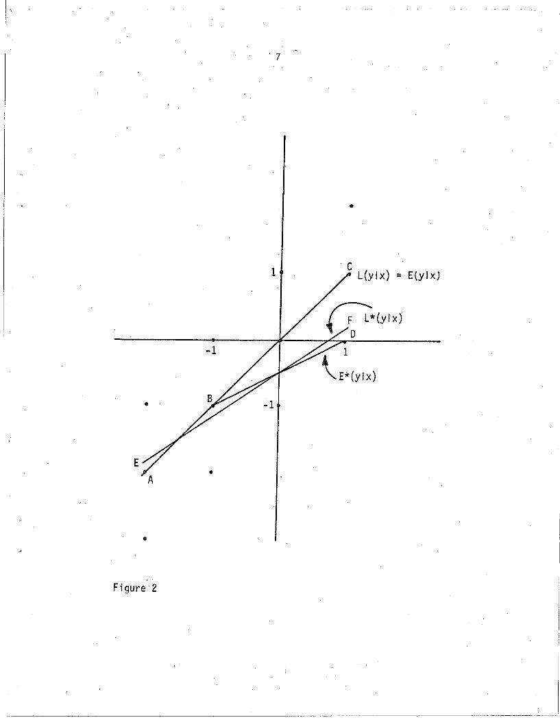
Example 2. In the second example, there is again a single x, but

the population consists of the twelve equi-probable points displayed in

Table 2.

Table 2

xy

12

5

y

Figure 1

L(yJx) = E(ylx)

L*(ylx) = E*(ylx)

x

6

The conditional expectation function is again

E(y Ix) x = L(y!x) (10)

"

which appears as the line AC in Figure 2. Again form the truncated

population by deleting points at which y is greater than zero. This

time, the conditional expectation function in the truncated population

[E*(y!x)] is not linear. This function is labeled ABD in Figure 2. We

can readily calculate L*(y!x), the best linear approximation to E*(ylx).

Using the results

E*(y)

we conclude that

-1.11

.988

-.889, C*(x,y) = .679 ,

(11)

L*(ylx) = -.500 + .688x

which is graphed in Figure 2 as EF.

(12)

As in the first example, linear regression in a sample from the

truncated population yields a biased estimate of the slope of L(ylx).

If b* is such a linear regression estimate, we know that

E(b*) =.688 I 1 . (13)

Next, we turn to a simple case of the classical normal regression

model where there is a single regressor z with a unit coefficient:

y=z+E:

2E: '\; N(O,O" ) . (14)

I_____________________________________________1

•

E

•

Figure'2

-1

•

, 7

1

-1

•

, CL(ylx) = E(ylx)

8

This model implies that the conditional distribution of y given z is

normal with mean z and variance a2• The probability density function

for y is

g(y) = (15)

The conditional expectation function is linear in z so it coincides

with L(ylz):

E(ylz) = L(ylz) = z . (16)

Now, consider the truncated subpopu1ation which consists of all

points at which y is less than some value H. In that subpopu1ation,

the density function for y is

{

g(y) /G(H)"g*(y) =

o

for y < H

otherwise(17)

where G is the cumulative normal distribution function

G(H) Hf g(y)dy_00

2 (18)

In the subpopulation, the conditional expectation of y given z is

E* (y Iz)Hf yg*(y)dy

_00

1 H= G(H) f yg(y)dy

_00

1 H (= G(H) _~ g(y)z dg(y)) dydy

9

z H a2H

= G(H) f g(y)dy - G(H) f dg(y)_00 _00

= z2.£Q!l 3

- a G(H)/'

(19)

so

Then

To study E*(y!z) it is convenient to transform variables. Let

a = (H-z)/a

z = H - aa •

(20)

(21)

.£Q!l _ f (a) _a G(H) - F(a) - rea) ,

(22)

say, where fee) and F(e) are the standard normal density and cumulative

functions respectively. Then (19) can be rewritten as

E*(Ylz) = z - area) • (23)

Evans (1975) has calculated rea) for various values of a. His graph of

rea) is reproduced in Figure 3 and is used to plot E*(ylz) in Figure 4.

Note that E*(y!z) is a positive, convex function of z which asymptoti­

4cally approaches y = z as a + _00 and y = L as a + 00.

The best linear approximation to E*(Ylz) is L*(Ylz) which has

slope equal to C*(z,y)/V*(z). Using

C*(z,y) = C*[z,E*(ylz)]

and (23), we obtain

.~-----~~------- ~~~~

(24)

10

· t

-3

Figure 3

-2 -1 1 2

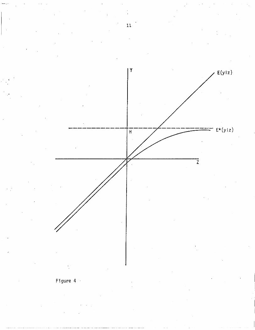
Figure 4

11

y

H

z

E(y Iz)

12

C*(z~y) = C*[z,z - area)]

which can be rewritten as

C*(z,y) = v*(z) - aC*[z,r(a)].

Note that rea) is monotonically decreasing in a and therefore mono-

(25)

(26)

tonically increasing in z. The sign of C;~[z,r(a)] can be determined

using a theorem due to Gurland (1967) regarding the covariance of

functions of random variables. Gurlandls theorem says that two mono-

tonically increasing (or decreasing) functions of the same random

variable will have a positive covariance. Since z and rea) are two

monotonically increasing functions of z, C*[z, rea)] is positive and

s* = C*(z,y)v*(z)

< C(z,y) =v(z)

1 . (27)

Once again we see that a linear regression coefficient estimate from a

sample drawn from a truncated subpopulation will be biased for the

slope of L(ylz) because L*(ylz) has a different slope. Next, we

generalize this result to the case of multiple regressors.

Consider the model

y = Xl S + s

2s 'U N(O,a ) ,

where x is a k x 1 vector of exogenous variables. The results contained

in our laSt example can in large part be generalized to cover this case

by defining

z - Xl S (29)

13

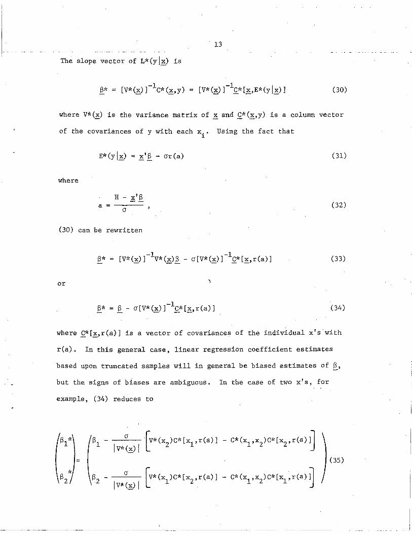
The slope vector of L*(Ylx) is

(30)

where v*(~) is the variance matrix of ~ and .Q.*(~,y) is a column vector

of the covariances of Y with each

E*(yl~) = Xl~ - area)

where

x ..1

Using the fact that

(31)

a =

H - XIS

a (32)

(30) can be rewritten

or

S* -1 -1[V1' (~) ] v* (x)~ - a [v* (x) ] c* [~, r (a) ] (33)

-1~* = ~ - a[v*(x)] C*[~,r(a)] (34)

where .Q.1' [~, r (a)] is a vector of covariances of the individual Xl s with

rea). In this general case, linear regression coefficient estimates

based upon truncated samples will in general be biased estimates of ~,

but the signs of biases are ambiguous. In the case of two x's, for

example, (34) reduces to

s ­1

S ...2

(35)

I

I·

14

The signs of bias will obviously depend upon the signs of the three\

. 5covarlances.

In this section, we have considered several examples of the biased

coefficient estimates which result when linear regression is applied to

truncated samples. We have found it useful to think of truncated

samples as random samples from truncated populations. Our conclusions

are that linear regression in truncated samples provides biased

estimates of the slopes of L(yl~) and that the directions of such

biases are, in general, ambiguous.

3. Consistent Estimation Techniques for Truncated Samples

In this section, two methods for obtaining consistent estimates

from a truncated sample are considered. The model is that of (28),

which we rewrite as

y = x '13 + Et -t - t

2E

ttV N(O,G ) •

t 1, .• • • , T (36)

The sample consists of all observations for which

y < Ht t

t = 1, •.. , T . (37)

The limit value H may vary across observations, but it is knoWn att

each observation.

a. Instrumental Variable Approach

Amemiya (1973) studies the model:

o

Y~ =r'~: £~

E:~ 'V N(O,w2

)

(38)otherwise t = 1, . . . , T

owhere Yt is the observed value of the dependent variable at observation

t, ~~ is a vector of exogenous variables, and E:~ is a normal disturbance

owhich is independent of xt . This is the specific case of the Tohit model

(Tobin, 1958) in which the lower bound is equal to zero at each observa-

tion.

Amemiya @bt~~ns cons~SEent estimates of this model using only the

non-limit observations. He shows that

oy'xo 0 --1:

E*(Yt) = y'x + wr(--)--1: w

and that

(39)

oy'xo 2 0 - -1: 2

= (y '~,.J + wy'x r(--) + wl. --1: W

002= y'x E*(y ) + w- -t t

(40)

where r is defined in (22). Defining

and

(42)

16

(40) implies

where

a 2 a a 2(Yt

) = y'x (y - u ) + w + v--t t t t

a a 2= y'x y + w + n--t t t

av - y'x ut --t: t

(43)

(44)

2Amemiya uses (43) to obtain estimates of y and w. The correlation

between nand y precludes linear regression, so Amemiya proposest t

A

a 0instrumental variable estimation of (43) with (x y ,1) as instruments

-tt

where

[~J (Y~) 2 (45)

"0 0'= xYt -t (46)

and where ~+ indicates the sum over all observations at which y~ is

"2 2greater than zero. He shows that:r.. and ware consistent for.:r.. and w

under general conditions.

The model displayed in (44) can be written in the form of (46) by

making the substitutions

oYt = Lt - Yt

~ = (-::) ,

p (:),

(47)

(48)

(49)

2w

-E:t

2o

17

.(50)

(51)

So, consistent instrumental variable estimates of our model can

be obtained using Amemiya's instrumental variable technique. First,

the Yt'S are regressed on the ~'s, and the predicted values from the

regression, Yt's, are used to compute (Ht

- Yt ) for each t. Next the

vectors ~ and ~ are constructed where

(H -y ) (L )t t t

~

and

(52)

d = (H -Y )-t t t (53)

Each element of c is regressed on d and a constant to obtain a-t -t

vector of predicted va1ues~. Finally, we regress (Yt)2 - 21 on

(22 , . , ck+1) and a constant; the coefficients obtained for

(22 , ••• , 2k+1) will be -S and the constant coefficient will be

"2cr. This procedure takes advantage of the familiar computational

technique fox obtaining instrumental variable estimates using a two-

stage linear regression algorithm.

b. Maximum Likelihood Approach

Amemiya (1973, p. 1000-1001) also spells out the maximum 1ike1i-

hood method for estimation of the model in (38) which can be adapted

as follows. The model displayed in (36) implies thaty is normallyt

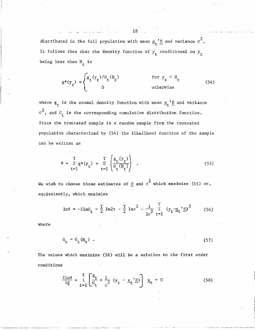
18 _ _

2distributed in the full population with mean x 's and variance a .-t -

It follows then that the density function of Yt conditional on Yt

being less than H ist

for y < Ht t

otherwise(54)

where g is the normal density function with mean x 'S and variancet -t -

2o , and Gt

is the corresponding cumulative distribution function.

Since the truncated sample is a random sample from the truncated

population characterized by (54) the likelihood function of the sample

can be written as

TIT g)\: (y )

t=l t

TIT

t=l(55)

2We wish to choose those estimates of £ and 0 which maximize (55) or,

equivalently, which maximize

1n<lJ

where

(56)

(57)

The values which maximize (56) will be a solution to the first order

conditions

dln<P - ~ [gt + 1:- (y - X 'S)J x = 0afi - t=l· Gt 0 2 t -t - =t

(58)

19

where

(59)

The secend de.rivatives _0£ __(58) ar.e displayed in the appendicx.

For a given set of data, we wish to find a solution to equations

(58) at which the likelihood function takes on its maximum value. To

do so, an algorithm for t~e maximization of a function of several

variables is required. The method used here was developed by Davidon,

described by Fletcher and Powell. (1963), and made operational by

Gruvaeus and Joreskog (1970). The method searches for a maximum of the

likelihood function using analytical first derivatives of the function'

and an approximation to the matrix of second derivatives, beginning

with user supplied starting values of the parameters. We will use the

instrumental variable estimates as these starting values. Having

found the maximum likelihood estimates of Sand 02

, we estimate the

asymptotic covariance matrix of these estimates as the negative of the

inverse of the matrix of second derivatives of 1n~. Under certain

2regularity conditions, the maximum likelihood estimates 6f S and a

are asymptotically efficient and asymptotically normally distributed

with means Sand 02 and variances estimated as noted above.

In this section two techniques for the estimation of simple

linear models from truncated samples have been described. The maximum

likelihood estimates have more desirable asymptotic properties, but the

choice of techniques in finite samples remains open. The instrumental

20

variable estimates have the practical advantage of being relatively

easy to compute. Both techniques are used in the following sections.

4. A Model of the Determination of Earned Income

In order to get an empirical picture of the relation between

full-sample and truncated-sample results we estimate an earnings

function using a full random sample and a truncated subsamp1e. The

model to be estimated determines earned income of male heads of house­

holds. The earnings function is not a structural equation but, rather,

represents a·reduced form equation associated with an unspecified

structural system of the demand for and supply of labor. The argu­

ments of the earnings function are exogenous variables which affect

demand and/or supply. Among these variables are factors which deter­

mine the individual's productive potential such as his age, his

education, and his intelligence. Other arguments of the earnings

function are family size which should affect labor supply, race which

captures earnings differences due to discrimination, and region which

should measure earnings differences attributable to regional varia­

tions in the productivity of labor and the cost of living.

Our model of earnings is

E = So + Sl GRSCH + S2 HSCH + S3 SOME + S4 GRAD + Ss TEST

+ S6 AGE + S7 AGESQ + S3 RACE + S9 SOUTH + S10 FSZ + E (60)

where-

E = ,individual's labor income in 1968 (includes imputed earnings

of self-employed)

GRSCH

HSCH

SOME

GRAD

21

=jl if individual did not enter high school

\? ~therwise (base category is high school graduates with no

further formal education)

if individual entered high school but did not graduate

otherwise

if individual graduated from high school, had further formal

training, but did not graduate from college

otherwise

if individual graduated from college

otherwise

TEST = individual's score on a sentence completion (IQ) test6

(scores range from 0 to 13)

AGE

AGESQ

RACE

SOUTH

FSZ

= individual's age in years

=Jio

- if individual is nonwhite

~ if individual is white

=ji if individual lives in the Southern Census Region

~ otherwise

= number of persons in the individual's household

2and E is a normal disturbance with mean zero and variance cr. We assume

that E is independent of the exogenous variables in the model.

Two characteristics of the functional form are worthy of note.

First, the model contains four dichotomous variables which measure the

individual's education. The education variable was originally available

in nine categories. For the sake of parsimony, we have collapsed these

nine categories into five categories. Second, we have specified a

-~~---~~----------------------------------------------------- --------------~--------------------- -j

22

quadratic form for the partial impact of age upon earnings pecause

most researchers have found age to have a first positive and then

negative effect upon earnings, a result which has theoretical appeal.

5. Data

The data used in this analysis were taken from the five-year

panel collected by the Survey Research Center (SRC) of the Institute

for Social Research at the University of Michigan. This data set

consis~s of five annual interviews with approximately 5000 family units,

40 percent of which were selected from members of the Survey of

Economic Opportunity (SEO) sample. The remaining 60 percent of the

sample units make up a national cross-sectional sample." In the present

paper the SEO follow-up sample is excluded. One-half of the national

cross-sectional sample has been randomly selected for analysi$; the

remainder is available for future analysis. Finally, attention is

restricted to male-headed families which had the same head over the

entire five-year period; a sample of 864 families is available. This

sample is assumed to be a random sample from the full population of

male heads of households.

A truncated subsample was constructed from the sample of 864

observations by excluding an observation if the family's income was

more than 150 percent of the family's poverty threshold ("O rshansky

Ratio" greater than 1.5). For a given family size this restriction

imposed an upper bound on total family income. A group of 253 obser­

vations remained. The sample is truncated on the basis of total family

income and the model explains only head's labor income, so we must

_ 2.3 ..

translate the truncation on family income into a truncation on head's

labor income. To do so, it is assumed that all other components of

family income are fixed. The upper bound on family income in the

truncated sample is 150 percent of the family's poverty threshold.

The upper bound on head's labor income is taken to be the family income

bound minus family income from sources other than the head's labor

income.

The full and truncated sample means and standard deviations of

the variables in our model are displayed in Table 3. Note that men

in the truncated sample have, on average, much lower earnings, much

less education, and only slightly lower intelligence test scores.

The average man in the truncated sample is slightly older than the

average man in the full sample. Further, we see that the proportions

of nonwhites and of southerners are higher in the truncated sample.

Finally, there is the interesting result that the average family size

is virtually the same in the two samples. One might have thought that

larger families with higher poverty thresholds would be over-represented

in the truncated sample, but such is not the case. Apparently, larger

families have sufficiently higher incomes that they are no more likely

to fall below the bound of 150 percent of their poverty thresholds.

6. Estimation of the Model

Four sets of estimates of the parameters of the earnings model

shown in (60) are described in this section. The first set, hereafter

denoted LR-F, was obtained with the full sample using linear regression.

The remaining three sets of estimates were obtained with the truncated

Table 3

Sample Means and Standard Deviations from the Full Sample and the Truncated Sample

Full Sample Full Sample Truncated Sample Truncated SampleMean Standard Deviation Hean Standard Deviation

E 7100. 5920. 2340. 2410 .

GRSCH .264 •441 .482 .501

HSCH .153 .360 .150 .358

SOME .244 .430 .194 .396

GRAD .152 .359 .059 .237

TEST 9.72 2.16 8.89 2.51

AGE 45.2 15.7 50.6 19.3

RACE .101 .301 .174 .380

SOUTH .338 .473 .466 .500

FSZ 3.47 1. 73 3.42 2.17

ISample Size 864 253

N.j::-.

25

sample using linear regression (LR-T), the instrumental variable

technique (IV-T), and the maximum likelihood technique (ML_T).7 These

four sets of estimates are displayed in Table 4; estimated standard

errors are reported in parentheses.

First, consider the LR-F estimates. The education variables

appear to have a strong impact upon earnings. It is somewhat surprising

that the coefficients of HSCH and SOME are not significantly different

from zero. This result implies that the earnings of high school

graduates are not significantly different from the earnings of those

who completed only some high school or from those who graduated from

high school, had some formal training beyond high school, but did not

graduate from college. The hypothesis that the coefficients of the

four education variables are jointly equal to zero can be tested with

an F-test. The F-statistic with 4 and 853 degrees of freedom is 32.9

which allows the hypothesis to be rejected at the .001 level of signi­

ficance. The age-earnings profile implied by the model exhibits a

positive effect of increasing age until age 46~ The variable RACE has

a negative but insignificant impact upon earnings. The lack of

significance may be due to the heterogeneity of the nonwhite group

which includes Orientals as well as Blacks and people of Spanish

heritage. The variable SOUTH has a strong negative impact upon

earnings. The family size variable has a strongly significant and

positive impact upon earnings, which might suggest that heads

with responsibilities for larger families are likely to be more

highly motivated to work or that richer people have more

children, in which case the model is mis-specified. The

~~------~----------------_.

26

Table 4

Estimates of the Earnings Model(Standard errors in parentheses)

Full Sample Truncated Sample

Linear Instrumental MaximumLinear Re ression Re ression Variabl~. Likelihood

CONSTANT -10,100. 47.9 4,220. 821.(1,600. ) (957.) (4,420.) (1,640.)

GRSCH -2,410. -879. -2,850. -1,460.(524. ) (342. ) (2,020. ) (588.)

HSCH -563. -172. -1,010. -840.(558. ) (401. ) (2,000.) (692.)

SOl1E 487. 213. 178. 702.(494. ) (382. ) (2,220.) (711. )

GRAD 4,140. 152. 3,680. 605.(561.) (521. ) (2,670.) (976. )

TEST 275. -27.9 44.2 -22.0(85.5) (47.1) (180.) (72 .1)

AGE 680. 110. 231. 172.(62.4) (37.2) (1)0. ) (62.4)

AGESQ -7.45 -1.50 -2.84 -2.27(.656 ) (.373) (1.67) (.605)

RACE -764. -273. -864. -418.(560.) (292.) (926. ) (448. )

SOUTH -909. -25.9 -239. -52.8(350. ) (215. ) (794. ) (353. )

FSZ 344. 545. -53.4 373.(104. ) (56.2) (258.) . (89.8).

a 4,710. 1,580. 3,140. 1,950.(136. )

R2

.367 .569

'I,

27

intelligence test variable has a positive coefficient which is differ-

ent from zero at the .01 level of significance. Finally, it should be

noted that this model fits the data remarkably well for a cross­

2sectional individual model as indicated by the R of .367.

The three sets of estimates of the coefficients of our model based

upon the truncated sample differ considerably. The linear regression

2estimates are inconsistent for Sand cr , but the biases cannot be

calculated explicitly as the true values of the parameters are unknown.

In addition, the calculated standard errors of the linear regression

estimates are spurious. It is interesting nevertheless to compare the

three sets of estimates from the truncated sample with the estimates

from the full sample.

First, comparing the linear regression estimates from the two

samples, note that the sign of each coefficient is ,preserved except

for the TEST coefficient. Second, of the remaining coefficient

estimates, the LR-T estimates are closer to zero than the LR-F esti-

mates with the single exception of the coefficient on FSZ. This

single exception makes sense if we remember that larger families had

higher income cut-offs due to the truncation on the "OrshanskyRatio."

Third, the ordering of the estimates of the education coefficients are

different in the two samples. In the full sample, a monotonically

increasing relationship exists between education and earnings, but in

the truncated sample it appears that college graduation reduces

earnings. Fourth, the age-earnings profile based on the truncated

sample is flatter and has an earlier peak at age 37. Finally,the

conventional estimate of the standard deviation of E is smaller in the

2truncated sample, and the R is larger. Generally, it seems that

28

linear regression on the truncated sample yields quite unsatisfactory

estimates of the coefficients of the earnings function, judging on the

basis of comparison with the LR-F estimates.

The instrumental variable estimates of the model seem to be more

satisfactory. The sign of each coefficient is the same as in the full

sample regression, except for FSZ, a somewhat puzzling exception. The

magnitudes of the IV-T coefficients tend to be closer to the magnitudes

of the LR-F estimates than are those of the LR-T estimates. In spite

of these similarities the instrumental variable estimates are subs tan-

tially different from the full sample estimates, but there is no

apparent pattern to the differences. Once again, we see a monotonic

relationship between earnings and education.

Turning to the maximum likelihood estimates, we see that the

estimated TEST coefficient is, once again, negative while the estimated

FSZ coefficient is positive. The signs of the other maximum likelihood

estimates correspond to the full sample estimates. The ordering of

the estimated coefficients of SOME and GRAD are as they were in the

set of linear regression estimates from the truncated sample, implying

'. a non--monotonic relationship between earnings and education. Generally,

the ML-T estimates are closer to the LR-F estimates than are the LR-T

estimates but not so close as are the instrumental variable estimates.

To test the hypothesis that the coefficients of the education variables

are jointly equal to zero, it is convenient to use a likelihood ratio

test. Recall that

-2 In(

<;pHO)<;Pm (61)

null hypothesis, in this case four.

29

where ~HO is the value of the likelihood function under the null hypo­

thesis, ~Hl is the value of the likelihood function under the a1tern~­

tive hypothesis, and k is the number of restrictions imposed by the

2The X statistic is 220, which

allows the hypothesis that education has no effect on earnings to be

rejected at the .005 level of significance.

Our maximum likelihood estimates are based upon two assumptions:

that there is no systematic difference between the truncated and full

populations apart from that due to truncation and that the stochastic

term in that function has a normal distribution conditional on the

values of the exogenous variables. We can test the first assumption

under the maintained hypothesis that the second is correct by means

of a likelihood ratio test. In order to perform this test we evaluate

the likelihood for the truncated sample using the LR-F and ML-T esti-

2 2mates of Sand cr. When we do so we obtain a very large X statistic

with twelve degrees of freedom of 1642 which forces the rejection of

the first assumption (conditional on the normality of E) at a level of

significance very close to zero.

If the second assumption is incorrect, however, this test is

difficult to interpret. ~What is required is a test·of the conditional

normality of the disturbance term in the full sample. The predictedA

values (E's) and residuals associated with the LR-F estimates were

computed. The observations were then grouped into deci1es on the

basis of the predicted values. 2Within each decile a Pearson X test of

the hypothesis that the residuals were distributed normally was

performed (Blum and Rosenblatt, 1972, pp. 408-409). The residuals in

2each decile were sorted into eight cells for this test, so the X

30

statistic has seven degrees of freedom. The cell boundaries were set

such that the probability of a residual falling into any cell, under

the null hypothesis, was .125. Table 5 reports the cell frequencies

of the residuals and the X2

statistic for each decile. The 5 percent

. . 1 1 f 2. h d f f d . 14 1 dcr1t1ca va ue or a X W1t seven egrees 0 ree om 1S ., an

the 1 percent critical value is 18.5. The assumption of normality

cannot be rejected for five deci1es at the 1 percent level of signifi-

cance and for two deci1es at the 5 percent level. One would have to

agree that the assumption of normality is somewhat tenuous.

7. Conclusions and Extensions

In this paper the problems encountered in using linear regressio~

to estimate simple linear models from truncated samples have been

examined. Two techniques for obtaining consistent estimates in such

situations were described. Finally, these techniques were'used to

estimate an earnings function with an artificially truncated sample.

There are two lessons to be learned from this exercise.

First, it is clear that linear regression will not, in general,

provide consistent estimates of linear models when samples are

truncated on the basis of the dependent variable. Empirically, it

appears that this problem may be of substantial magnitude as it seemed

to be in the example.

Second, we cannot be too optimistic about the possibility of

using the Rural Income Maintenance Experiment data to estimate the

earnings, model as it now stands. We can obtain consistent estimates

from truncated samples only if the model is correctly specified, and

31

Table 5

Goodness of Fit Tests of the Normality of the Disturbancein the Earnings Equation

Decile of E Cell Frequencies (Low to High)

(Low to High) 1 2 3 4 5 6 7 82

X

1 .00 .00 .19 .24 .22 .10 .19 .06 46.1

2 .00 .13 .21 .21 .19 .15 .10 .01 32.7

3 .00 .17 .16 .23 .21 .14 .05 .03 36.2

4 .05 .19 .19 .23 .13 .16 .03 .02 31. 0

5 .03 .13 .23 .19 .20 .16 .05 .01 33.8

6 .06 .13 .14 .22 .16 .15 .08 .06 15.4

7 .06 .13 .15 .21 .21 .09 .07 .08 17.4

8 .13 .09 .16 .23 .17 .05 .09 .07 18.4

9 .09 .09 .16 .17 .13 .19 .06 .10 10.0

10 .10 .17 .19 .09 .09 .11 .08 .18 10'.3

/

32

this model appears to be misspecified. Nevertheless, techniques have

been proposed which will provide consistent and possibly asymptotically

efficient estimates of correctly specified models using truncated

samples. Obviously, it is best to use full samples when they are

available, but truncated samples contain information which economists

cannot afford to waste.

The maximum likelihood technique developed in this paper can be

easily extended, to the estimation of multiple equation models.

Joreskog (1973) has developed a maximum likelihood technique for the

estimation of a general linear model. Most types of linear models

can be expressed in the form of Joreskog's model. The model implies

a joint mu1tinorma1 distribution of observed exogenous (x) and endog-

enous (y) variables. Each specific model implies a set of restrictions

on the covariance matrix of the variables, as the elements of the

matrix are functions of the parameters of the model. These parameters

can be estimated from a random sample via the maximization of the 1ike-

1ihood function

T<I> = II m(x ,Yt)

t=l -t(62)

f'

where m is the mu1tinorma1 density function. Consider a sample that

exceeded some predetermined va1ue,H .t

'"

has been truncated when Y1t

likelihood function for the Joreskog model would then be

The

<I>* (63)

·.. . .......-.. , ... ....~".. ._,-.._~.... ~. .

33

where MI

is the marginal cumulative distribution of YI' Estimates of

this model can be obtained from truncated samples by finding parameter

values which maximize (63).

Having developed techniques for the estimation of multiple equa-

tion models from truncated samples, we can formulate a more plausible

structural model of the determination of earnings. One such model

might be

In S = a In W+ ~'~l + 8

In W = y'Z + ()J--z

In E = In S + In W

(64)

(65)

(66)

where S is hours worked, W is the individual's wage rate, E is the

individual's earnings, and ~l and !z are vectors of exogenous variables.

Equation (64) is the demand function facing the individual and equation

(65) is the supply function of the individual.· The identity (66)

permits the possibility of an earnings truncation in this model.

The multiple equation technique can also be used for the estima-

tion of models which more fully exploit panel data. One such model is

y* = S'Z + 8!'

y. = yi~ + V.J J

j I, . . . , J (67)

where! is a vector of exogenous variables, y* is permanent income,

and Y. is measured income in period j. If such a model is to be. J

estimated with income maintenance experiment data, then the truncation

on first period income should not be ignored. The technique suggested

above will allow us to account for the truncation.

fe.

34

NOTES

lAfter completing an earlier draft of this paper, I became aware

of a paper by Hausman and Wise (1975) which deals with this same

subject in a similar fashion.

2This density function may remind the reader of the Tobit model

~eveloped by Tobin (1958) and analyzed by Amemiya (1973). The differ-

ence between the two models is that the Tobit model implies a nonzero

probability of limit observations while our model implies a zero

probability of such observations.

3Johnson and Kotz (1970, Vol. 1, p. 81) display the eXPected

value of the doubly truncated normal distribution, which can be

simplified to (19) when the lower truncation point is minus infinity.

4 F" . 3 h (). d . f . f bIn i1gure , we see t atr a 1S a ecreas1ng· unct10n 0 a, ut

we can obtain this result analytically. Differentiating rea) we

obtain

d[r(a)] 1 '\~aF (a) f (a) _ [f(a)]2)=da [F(a)]2

= _ .!J& [ + f(a)]F(a) a F(a)

,.,~,

= -r(a) [a + rea)] • (Fl)

Since rea) is strictly positive everywhere, the sign of (Fl) will be

determined by the sign of [a + rea)]. When a is greater than or equal

to zero [a + rea)] is obviously positive.

than zero, we define

In the case wheret is less.. .

so that

35"

u -a (F2)

a + rea) = -u + r(-u) u > 0 • (F3)

Using the symmetry of the normal distribution we conclude that

r(-u) = f(-u)F(-u)

feu) 1= l-F(u) = R(u) (F4)

where R(u) is Mills' Ratio (See Johnson and Kotz, Vol. 2, p. 278). So

for a less than zero

a + rea) + _1_-u R(u) u > 0 . (F5)

Since M1lls' Ratio satisfies the inequality (Johnson and Katz, Vol. 2,

p. 279)

-~:

o < R(u) < 1:­u

we know that

1R(u) > u

1-u + R(u) > 0

a + rea) > 0

u > 0

u > 0

u > 0

u > 0 .

, (F6)

(F7)

Having established that a + rea) is strictly positive everywhere, we

conclude that d[r(a)]/da is negative for all values of a~

5Goldberger (1975) has shown that the signs of the biases are

ambiguous.

p

'JI

36

6This test consisted of 13 items selected from the verbal part of

the Lorge-Thorndike Intelligence Test.

7Linear regression estimates were obt~ined using the Regan 2

program in the Statjob series. Instrumental variable estimates were

calculated using the Time Series Processor available fromDACC.

Maximum-likelihood estimates were obtained using a minimization program

written by Gruvaeus and Joreskog and adapted by me.

37

APPENDIX

To derive the first and second order conditions for the maximiza­I!I

tion of (64) we have made use of several results:

(AI)

ClGt-- =

Clcr2(A2)

Clg 1___t = __ (L' - x 'S)g xo~ cr2 t -t - t-t

(A3)

2­- x 'S'--t "':".J

2cr4(A4)

The first order conditions are displayed in (66). The second derivatives

are as follows:

G+~ rL

2 L t-cr_l..-Jxx'2 -t-tcr

T [g "(GL: ttL

t=l 2a2G~ cr2 [ t

(y -x 'I3>Jt -t--" x

cr4 -t

- x 'SJ 2 - G - + -g [L-t- , t t t -~'~)

(AS)

2 TCl Inc]? = ~'Z Z '"

ocr Clcr t=l- G + g

t t

f.;

38

REFERENCES

39.

Johnson, Norman L. and Samuel Kotz. Continuous Univariate Distribu­

tions, Vol. 1-2, Houghton Mifflin Co., New York, 1970.

Joreskog, Karl G. "A General Method for Estimating a Linear Structural

Equation System," in Arthur S. Goldberger and Otis Dudley Duncan,

eds. Structural Equation Models in the Social Sciences, Seminar

Press, Inc., New York, 1973.

Survey Research Center. A Panel Study of Income Dynamics. Volumes

I-II, Institute for Social Research, University of Michigan, Ann

Arbor, 1972.

Tobin, James. "Estimation of Relationships for Limited Dependent

Variables." Econometrica, Vol. 26 (1958), pp. 24-36.