77
Nuclear Fuel Bundle Design Optimization using a Simplex Method Anders Haulin Supervisor: Jan Pallon, Ph.D. Department of Nuclear Physics, Faculty of Engineering Lund University August 2014
Nuclear Fuel Bundle DesignOptimization using a Simplex Method
Anders Haulin
Supervisor: Jan Pallon, Ph.D.
Department of Nuclear Physics, Faculty of Engineering
Lund University
August 2014
Abstract
A strategy for nuclear fuel bundle design optimization in boiling water reactors(BWRs),using a simplex method, is presented and examined. The objective of the study isto see how an automatic optimization scheme can create nuclear designs for use inBWR fuel bundles and how the scheme can be improved. Challenges with apply-ing linear simplex optimization to non-linear bundle physics lie in approximatingbundle characteristic parameters accurately while keeping calculation times down.Several areas for improvements are found in the calculations and investigation ofthese find that many can improve accuracy only at the cost of deteriorating calcu-lation time, whereas others such as utilizing symmetries can improve accuracy atno cost. The important R-factor is examined in detail and its implementation in asimplex optimization is studied and improvements to it suggested. It is found thatautomatic fuel bundle optimization using a simplex method can generate feasibledesigns and in some cases perform better than layouts made by nuclear designers.With simplex targets and constraints too narrowly specified they will however un-derperform in areas other than the target function. The reference design enteredinto the optimization is also shown to be of great importance to performance. It isfinally stressed that the optimization framework does have potential to improve thenuclear design process but needs a user with nuclear design experience to operatewell and an improved data-management system to be user-friendly.
2
Acknowledgements
I want to thank Sven-Birger and Simon for the idea of the project and the necessaryassistance to complete it, Sven and the BTF department for great support in astimulating environment and Mikael for sharp insights in optimization as well asnew angles and perspectives on the problems I faced.1
1I also want to thank Bitsy for being supportive and generally awesome.
3
Nomenclature
a The difference in k∞ at 0 GWd/tU burnup which would result fromremoving all BA from the design.
b The burnup at which maximum bundle k∞ occurs
Fint Internal power peaking factor: the maximum relative pin power inan axial fuel bundle segment.
k∞ The ratio of the neutron production rate and the neutron loss rate in aspecific fuel lattice under reflective (or periodic) boundary conditions.Used as a measure of a specific fuel bundle’s contribution to theneutron economy of a reactor.
P Relative pin power distribution: the power generated in a chosenaxial segment of a fuel rod relative to the average power in that axialsegment of the bundle.
R R-factor: a parameter used in CPR correlations as a measure ofbundle dryout sensitivity to changes in bundle power. The R-factoris a function of the fuel bundle relative pin power distribution.
BA Burnable absorber: an element with a high thermal neutron absorp-tion cross section, typically gadolinium, added to nuclear fuel to alterits characteristics.
bundle Boiling Water Reactor nuclear fuel bundle. An assembly of fuel rodsused to fuel the reactor.
burnup Nuclear engineering term for the amount of energy that has beenextracted out of a nuclear fuel.
BWR Boiling Water Reactor
CPLEX A commercial simplex optimization program used in this project.
CPR Critical Power Ratio: a reactor safety margin stating how muchpower can increase before inducing dryout conditions.
CPR correlation A set of equations correlating reactor parameters such as bundleR-factors, bundle power, axial power shape, bundle coolant flow andinlet sub-cooling into a measure of CPR.
DOFACT A program used in this project to calculate bundle R-factors for adryout correlation.
4
Nuclear Fuel Bundle Design Optimization using a Simplex Method
dryout A situation when heat flux from a BWR rod reaches a level whereboiling water can not cool sufficiently,water film on fuel cladding driesout and fuel rod temperature rises swiftly.
enrichment The weight fraction of 235U to total uranium within a confinement; inthis project normally a fuel rod or an axial segment of a fuel bundle
gap In a simplex optimization the gap is a measure of the discrepancybetween the incumbent best solution’s objective function value andestimation of global optimum’s. Gap tolerance prescribes how smallthis gap should be for an optimization to terminate.
lattice code A coarse-grid finite mesh program that calculates burnup-dependentfuel parameters k and P for bundle designs.
LHGR Linear Heat Generation Rate: a reactor parameter and constraint de-scribing heat generation per fuel rod length, in this project simplifiedas a constraint on Fint.
OPL Optimization Programming Language, a proprietary programminglanguage used to create optimization models.
PHOENIX A licensed 2D lattice code used in this project.
PLR Partial Length Rod, a fuel rod shorter than bundle length, typically1/3 or 2/3 the length of full length rods.
PWR Pressurized Water Reactor
reactivity Deviation from criticality: k 6= 1. Measured in pcm, pour cent milleor 1
100000, used to represent small changes in multiplication factor.
S-matrix Sensitivity matrix: a set of data describing the effects from changesin fuel bundle composition on fuel bundle characteristic parameters.
Simplex Simplex method, a deterministic optimization algorithm used for thisproject.
slice An axial bundle cross section in which 2D computations are per-formed; using axial slices at different heights along the bundle trans-fers 2D calculations to a 3D picture.
tolerance see gap
Chapter 0 Anders Haulin 5

Contents
1 Introduction 8
1.1 Nuclear Reactor Theory . . . . . . . . . . . . . . . . . . . . . . . . . 8
1.1.1 Nuclear Fission . . . . . . . . . . . . . . . . . . . . . . . . . . 8
1.1.2 Neutron Economy . . . . . . . . . . . . . . . . . . . . . . . . . 10
1.1.3 Boiling Water Reactors . . . . . . . . . . . . . . . . . . . . . . 11
1.1.4 Critical Power Ratio . . . . . . . . . . . . . . . . . . . . . . . 11
1.1.5 Uranium Enrichment and Burnable Absorber . . . . . . . . . 12
1.2 BWR Fuel Bundles . . . . . . . . . . . . . . . . . . . . . . . . . . . . 13
1.2.1 Mechanical Design . . . . . . . . . . . . . . . . . . . . . . . . 13
1.2.2 Nuclear Design . . . . . . . . . . . . . . . . . . . . . . . . . . 14
1.2.3 Fuel Bundle Characteristic Parameters . . . . . . . . . . . . . 16
1.3 The case for automatic optimization . . . . . . . . . . . . . . . . . . 19
1.3.1 The problem at hand . . . . . . . . . . . . . . . . . . . . . . . 19
1.3.2 Optimization strategies . . . . . . . . . . . . . . . . . . . . . . 20
1.3.3 The simplex method . . . . . . . . . . . . . . . . . . . . . . . 21
1.3.4 Other work in the field . . . . . . . . . . . . . . . . . . . . . . 22
2 Existing Optimization Strategy 23
2.1 Outline . . . . . . . . . . . . . . . . . . . . . . . . . . . . . . . . . . . 23
2.2 Constraints and objective . . . . . . . . . . . . . . . . . . . . . . . . 25
3 Method 27
3.1 Research Questions . . . . . . . . . . . . . . . . . . . . . . . . . . . . 27
3.2 Project Progression . . . . . . . . . . . . . . . . . . . . . . . . . . . . 28
3.2.1 Practical Issues . . . . . . . . . . . . . . . . . . . . . . . . . . 28
3.2.2 Improving the Approximations . . . . . . . . . . . . . . . . . 29
3.3 Two Optimization Cases . . . . . . . . . . . . . . . . . . . . . . . . . 29
4 Apparatus 30
4.1 S-matrix hardware and software . . . . . . . . . . . . . . . . . . . . . 30
4.1.1 Hardware . . . . . . . . . . . . . . . . . . . . . . . . . . . . . 30
4.1.2 Software . . . . . . . . . . . . . . . . . . . . . . . . . . . . . . 30
4.2 Simplex optimization hardware and software . . . . . . . . . . . . . . 30
4.2.1 Hardware . . . . . . . . . . . . . . . . . . . . . . . . . . . . . 30
4.2.2 Software . . . . . . . . . . . . . . . . . . . . . . . . . . . . . . 30
4.2.3 Equipment upgrade . . . . . . . . . . . . . . . . . . . . . . . . 31
6

Nuclear Fuel Bundle Design Optimization using a Simplex Method
5 Results 325.1 Evaluating the framework . . . . . . . . . . . . . . . . . . . . . . . . 32
5.1.1 Two-step approach . . . . . . . . . . . . . . . . . . . . . . . . 325.1.2 Symmetry issues . . . . . . . . . . . . . . . . . . . . . . . . . 335.1.3 Average enrichment implementation . . . . . . . . . . . . . . . 34
5.2 Improving approximations . . . . . . . . . . . . . . . . . . . . . . . . 355.2.1 k∞ . . . . . . . . . . . . . . . . . . . . . . . . . . . . . . . . . 355.2.2 Power distribution . . . . . . . . . . . . . . . . . . . . . . . . 405.2.3 R-factor . . . . . . . . . . . . . . . . . . . . . . . . . . . . . . 41
5.3 Optimized layout results . . . . . . . . . . . . . . . . . . . . . . . . . 515.3.1 BA rod position optimization . . . . . . . . . . . . . . . . . . 515.3.2 Uranium enrichment and Gd concentration optimization . . . 535.3.3 Performance compared to manual designs . . . . . . . . . . . . 55
6 Discussion 626.1 Simplex framework . . . . . . . . . . . . . . . . . . . . . . . . . . . . 62
6.1.1 Benefits of simplex fuel bundle optimization . . . . . . . . . . 626.1.2 Simplex method improvements . . . . . . . . . . . . . . . . . 636.1.3 Feasibility and performance of optimization . . . . . . . . . . 656.1.4 Recommendations and usage guidelines . . . . . . . . . . . . . 66
6.2 Project evaluation . . . . . . . . . . . . . . . . . . . . . . . . . . . . . 686.2.1 Goal attainment . . . . . . . . . . . . . . . . . . . . . . . . . 686.2.2 Method used . . . . . . . . . . . . . . . . . . . . . . . . . . . 686.2.3 Areas for further investigation . . . . . . . . . . . . . . . . . . 68
6.3 Project conclusion . . . . . . . . . . . . . . . . . . . . . . . . . . . . 70
7 Bibliography 71
A Additional Data 74
Chapter 0 Anders Haulin 7
Chapter 1
Introduction
1.1 Nuclear Reactor Theory
The goal of this thesis has been to study the performance and applicability of au-tomatically optimized nuclear designs for Boiling Water Reactor fuel bundles. Toexplain the setting of the problem a background in nuclear engineering is provided,more detailed background on nuclear physics can (amongst others) be found inKrane [22] and detailed knowledge on nuclear engineering in Lamarsh & Baratta[23].
1.1.1 Nuclear Fission
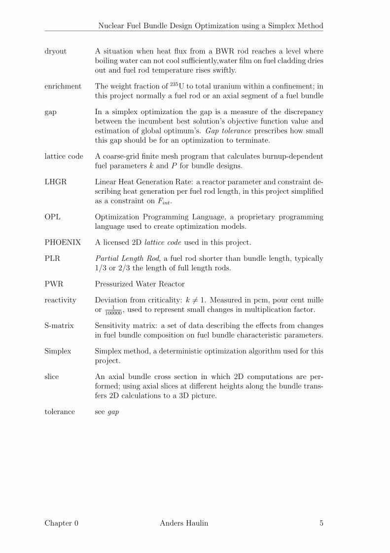
The underlying principle of all commercial nuclear power is nuclear fission. Nucleiare made up of nucleons combining through interplay between the strong nuclearforce supplying an attracting force between all nucleons and the electromagneticforce contributing a repelling force between protons. The general picture of the po-tential arising from these forces, although complicated in its details, can be displayedin a binding energy diagram (see Figure 1.1). The diagram in Figure 1.1 shows thebinding energy per nucleon in the nuclei from hydrogen to uranium. Omitting thelocal variations caused by quantum effects in nuclear structure we see a general trendof a sharp rise in binding energy per nucleon as light nuclei combine to form largercores. Fusing smaller cores into larger allows nucleons to bind more strongly to eachother thus releasing energy which of course is the fusion power that drives the sun.However, at A = 62 the slope of the curve changes as the marginal repulsion effectof increasing proton numbers overtake the marginal attraction of increasing nucleonnumber. This negative slope gives rise to a binding energy per nucleon in 235U whichis 13.7 % lower than that in 62Ni. Although forming elements with heavier cores thanthese cost energy it is possible and the earth’s crust contains substantial reserves ofaccessible elements with high nucleon numbers [7]. Nuclear fission energy is releasedas these heavy nuclei split and individual fission products form tighter bound nucleiin lower states of total energy. Following fission of a heavy element there is alsousually an emission of free neutrons, this is due to another nuclear structure effectthat can be visualized on the line of beta stability, Figure 1.2.
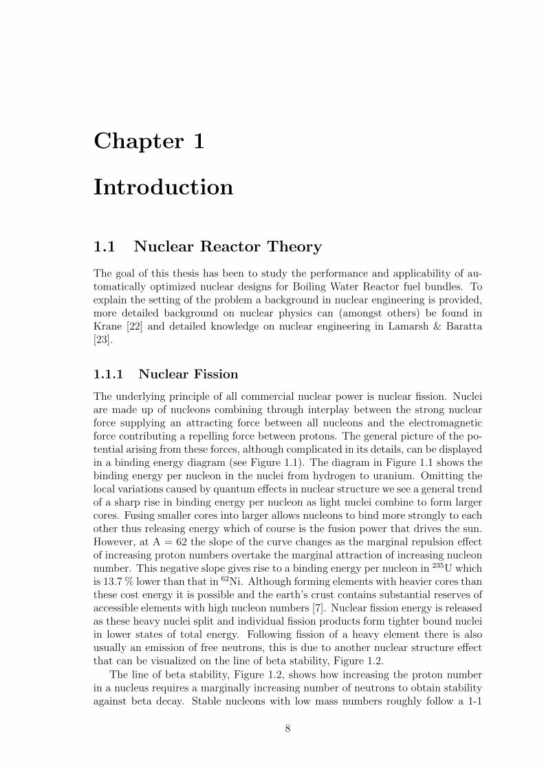
The line of beta stability, Figure 1.2, shows how increasing the proton numberin a nucleus requires a marginally increasing number of neutrons to obtain stabilityagainst beta decay. Stable nucleons with low mass numbers roughly follow a 1-1
8
Nuclear Fuel Bundle Design Optimization using a Simplex Method
Figure 1.1: Binding energy per nucleon for a large set of isotopes. NASA [5]
Figure 1.2: A large number of isotopes, black dots represent nuclei stable againstbeta decay. Note the trend towards more neutrons per proton in beta-stable nuclei.Brookhaven National Laboratory [6]
Chapter 1 Anders Haulin 9

Nuclear Fuel Bundle Design Optimization using a Simplex Method
ratio such as in 16O whereas the most abundant form of uranium, 238U, has 1.59neutrons per proton. This explains why common fission reactions such as Equation1.1 create lighter elements with neutron abundance and therefore release high energyneutrons.
23692 U→ 141
56 Ba + 9236Kr + 3 · 1
0n (1.1)
Although fission can occur spontaneously in heavy elements the most importantfission reactions in commercial reactors are the neutron-induced fissions of 235U and239Pu. These nuclei both have an even number of protons and odd number ofneutrons and a significant cross section for neutron absorption into an even-evennucleus1. This intermediary nucleus is created in a high energy state due to theabsorbed neutron; this makes it extremely likely to split. [22]
10n + 235
92 U→ 23692 U∗ → 141
56 Ba + 9236Kr + 3 · 1
0n (1.2)
Often the reaction 1.2 is written in compound form 1.3 to demonstrate how the236U is only an intermediary stage of 235U fission.
10n + 235
92 U→ 14156 Ba + 92
36Kr + 3 · 10n (1.3)
1.1.2 Neutron Economy
To obtain a sustained nuclear chain reaction useful for power production it is ofcourse a requirement that the neutrons required to induce a fission event are replacedby new neutrons from that fission reaction. In a thermal-neutron induced 235Ufission there are on average 2.44 new neutrons released [3]. This implies that thetotal loss of neutrons from phenomena such as leakage, neutron decay and neutroncapture in other elements (not inducing fission) must be approximately 59 % for thereaction to be stable. The state of neutron production in a reactor is described byits multiplication factor k: the ratio of the neutron production rate and the neutronloss rate. A reactor with k = 1 is said to be critical which means that the neutronflux is constant over time as one fission induces exactly one fission. A normallyoperating reactor as a whole will always be extremely close to k = 1, or criticality,as any deviations from k = 1 will create very fast swings in power multiplying overextremely short neutron regeneration timescales2, this would make the reactor hardto control. Since reactors are assumed to be very close to criticality a commonlyused unit3 for deviations from criticality (called reactivity) is the pcm, pour centmille or 1
100000, used to represent small changes in multiplication factor. The k value
for the whole reactor is normally denoted k-effective (k-eff) as it covers the balancebetween neutron production, neutron absorption and neutron leakage for the actualsystem. To describe the reactivity characteristics of individual fuel assemblies theterm k∞ (k-infinity or k-inf) is used. In this case an infinite reactor core with thespecific fuel lattice is created using reflective (or periodic) boundary conditions.
The k∞-values for individual fuel bundles and rods may be far above or belowcriticality, i.e. k∞ = 1 , contributing their share to the total k of the reactor.
1Even-even nuclei, with even numbers of both protons and neutrons are more stable than thosewith odd numbers due to quantum nucleon pairing effects, it is therefore likelier for an even-oddnucleus to absorb a neutron and become even-even than vice-versa.
2Mean neutron lifetimes in nuclear reactors range from 10-4 to 10-7 seconds, whereby a smalldeviation from criticality multiplies extremely rapidly.
3k is of course dimensionless.
10 Chapter 1 Anders Haulin

Nuclear Fuel Bundle Design Optimization using a Simplex Method
The concept of k∞ on the bundle-level will be explored in further detail in thenext chapter. As a reactor operates it fissions the nuclei loaded into its core forproduction of energy. In most commercial reactors a batch of fuel is inserted for acycle of 12-24 months and the core is kept closed without any possibility for additionor extraction of material during this time period. Throughout this cycle the reactorwill consume, or burn, its fissile 235U leaving a smaller and smaller fraction of thisisotope available for fission. This decreasing macroscopic fission cross section impliesthat the reactivity contribution from 235U would be steadily decreasing, seeminglyat odds with stable operation. Four of the factors solving this problem are:
• Neutron-induced transmutation of 238U to 239Pu generating new fissile mate-rial.
• Neutron-absorbing movable control rods that take up excess reactivity in thebeginning of the cycle to later be withdrawn.
• Addition of a burnable absorber (BA), such as gadolinium.
• Variation of core coolant flow to change moderation (void fraction in coolant).
Burnable absorber is of key significance to this project and its properties will befurther explained in Section 1.1.5.
1.1.3 Boiling Water Reactors
Among commercial light-water moderated nuclear reactors there are two very promi-nent classes of designs: pressurized water reactors (PWR) that use highly pressurizedlight water for cooling and boiling water reactors (BWR) that operate at a lowerpressure allowing the reactor water to boil.
There are many differences between the two kinds, notably the number of coolantloops (3 in PWR, 2 in BWR) and the operating pressure (∼70 atm for a BWR [1]and ∼159 atm for a PWR [2]). From a nuclear core design viewpoint there are afew principal features that make BWR’s interesting.
• The fuel bundle lattice contains inter-assembly gaps with non-boiling waterwhich makes the environment in which neutrons travel more heterogeneousthan that of a PWR fuel. Typically BWR designs feature greater numbers ofenrichment levels in more complicated patterns than PWR nuclear designs.
• The properties of the coolant water changes axially as it boils, the top regionof a fuel assembly will thus operate in higher void than the bottom region.This makes the fuel design in BWRs more 3-D dependent than in PWRs.
These traits of BWRs mean that there is a large scope for fuel designs to optimallyutilize uranium and burnable absorber material in the fuel and thus a good prospectfor optimization; to deliver favorable properties of the fuel assemblies. [23]
1.1.4 Critical Power Ratio
The large power density of nuclear reactors brings with it several cooling issuesrelated to the properties of the coolant water. In BWRs an important safety issue
Chapter 1 Anders Haulin 11
Nuclear Fuel Bundle Design Optimization using a Simplex Method
concerns Critical Heat Flux (CHF), the heat flux from a fuel rod at which the filmof liquid water present on the surface of the rod under good operating conditionscan not be sustained and no liquid water is available for surface boiling (and thuscooling). As long as there is enough water to sustain boiling an increase in heat fluxwill cause an increase in heat transfer through increased boiling. If the heat fluxrises too much, the water film can become broken up and large regions of insulatingvoid can occur. When this insulating void occurs the heat transfer rate from thefuel rod to its environment is strongly deteriorated. This dangerous phenomenonis also called dryout and when increased heat flux leads to decreased boiling heattransfer the rod temperature will rise dramatically; risking fuel damage. For anillustration of the speed at which temperature can rise during dryout, a commondefinition of dryout in experiment settings is a rod temperature increase of morethan 25 degrees per second [20]. Critical Power Ratio (CPR) is the ratio of theactual heat flux in the fuel and the CHF where dryout occurs, stating how much thepower can increase without reaching CHF. The value o the CHF depends heavily onthermal-hydraulic parameters and fuel design. Modern BWR fuel employs severaldetails to distribute water in an optimal fashion and the power distribution withinthe bundle is optimized for a good CPR performance. The interplay between CPRand bundle design through the important R-factor will be explained in greater detailin Section 1.2.3.4
1.1.5 Uranium Enrichment and Burnable Absorber
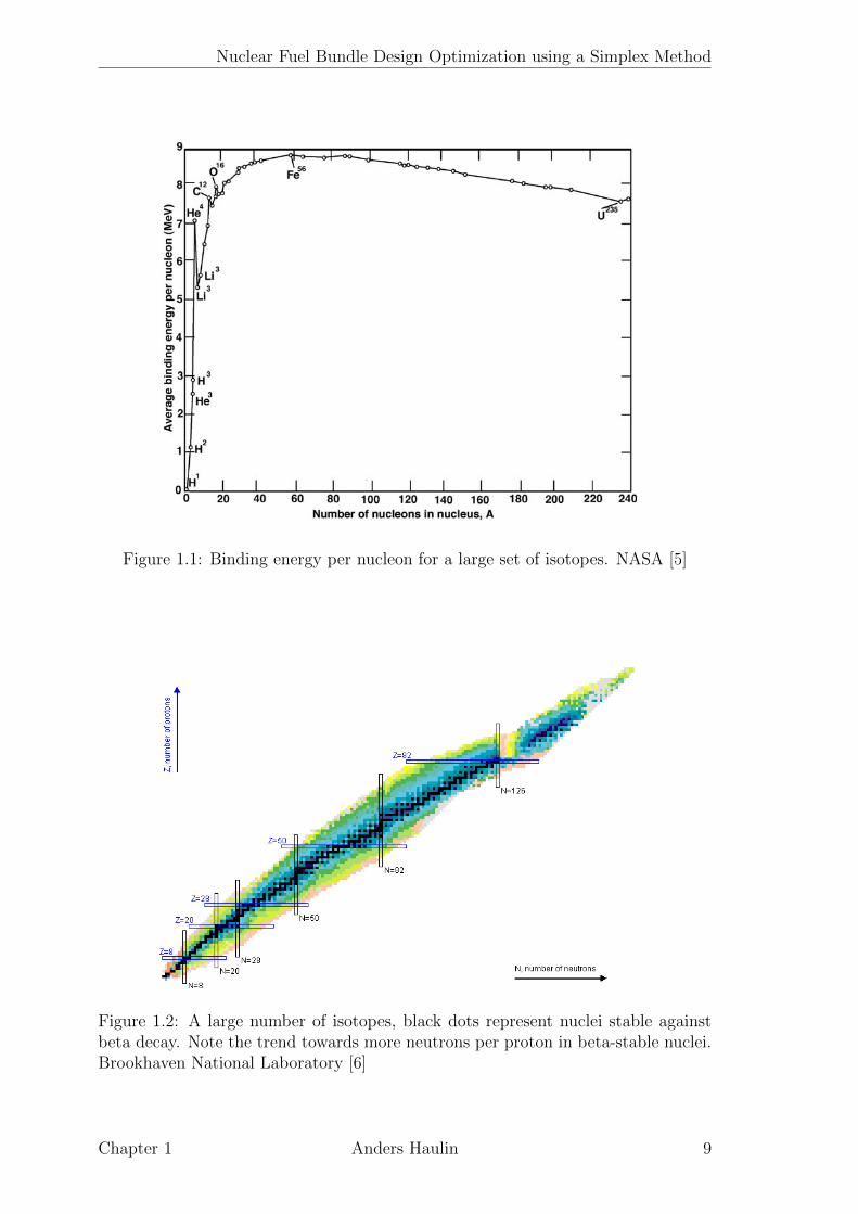
This project deals with optimizing two components over nuclear fuel bundle gridsto obtain optimal bundle properties. The components are uranium enrichments.Uranium enrichment refers to the percentage by weight of 235U in the uraniumcomponent in a certain area such as fuel rod, fuel bundle or the entire reactor core.The fuel assemblies considered in this project can have uranium enrichments fromnatural unenriched (0.71) up to 4.95 % 235U. Burnable absorber (BA) is an element,typically gadolinium, added to the nuclear fuel to alter its reactivity properties, seeexample in Figure 1.3. Burnable absorbers are isotopes that have very high thermalneutron absorption cross sections and can therefore decrease the fission-inducingneutron flux in their vicinity, see Table 1.1 for gadolinium thermal neutron capturecross sections. However, subsequent neutron absorptions during the reactor cycleeventually transmute the isotope into one with a much smaller absorption crosssection. The diminishing number of nuclei of absorbing isotopes means that thenegative contribution to k also decreases.
Thus the BA effect on k counters that of the enriched uranium, first loweringthe neutron flux but eventually decreasing its absorption effect, becoming “burntout”. Figure 1.3 shows how introduction of BA into a lattice drastically changes the
4The dryout safety concern in BWRs has a PWR analogy known as departure from nucleateboiling, DNB. Both situations concern a critical heat flux where cooling properties change starkly.The difference between the two lies in the ratios of steam and liquid water in the two reactor types:PWRs have cooling channels of mostly non-boiling water with boiling occurring at fuel rod surfaceswhereas BWR cooling channels contain mostly steam with films of water dispersed to cover fuelrods. DNB occurs when bubbles from boiling combine and form films that insulate the fuel rodsand the boiling regime changes from nucleate boiling to film boiling. The PWR CPR ”equivalent”called DNB ratio plays a similar role as CPR as a parameter to optimize to risks of dangeroussteep temperature increases.[26]
12 Chapter 1 Anders Haulin

Nuclear Fuel Bundle Design Optimization using a Simplex Method
the thermal 157Gd resonance ~see Table IV!. The thermalelastic scattering cross section for 157Gd has a large un-certainty since it is essentially the small difference oftwo large numbers ~total and capture cross sections!.Gadolinium-156 also exhibits a large deviation fromENDF in its small and statistically uncertain thermal elas-tic cross section. Gadolinium-156 has only two reso-nances below 100 eV. The increase in its thermal elasticcross section is due to the substantial increase in theneutron width of the 80 eV resonance ~see Table V!.However, the uncertainty on that neutron width ~seeTable V! encompasses the majority of the increase.
Resonance integrals ~Table VIII! are given for eachisotope as well as their contribution to the elementalvalues. The integrations extend from 0.5 eV to 20 MeV.The low-energy cutoff is above the thermal region dou-blet. The elemental resonance integral for Gd as mea-sured is 2.8% ~11 b! larger than that of ENDF. The largestfractional increases in isotopic contributions occur in154Gd and 158Gd; 154Gd and 158Gd have far fewer reso-nances than 155Gd or 157Gd. A 14% increase in the 158Gdresonance integral compared to ENDF was measured.This is dominated by the 22.3-eV resonance whose neu-tron width changed by approximately the same amount.
TABLE VI
Thermal Capture Cross Sections: A Comparison of ENDF0B-VI to RPI Results*
Thermal Capture Cross Sections
ENDF RPI
Isotope AbundanceThermalCapture
Contributionto Elemental Percent
ThermalCapture
Contributionto Elemental Percent
152Gd 0.200 1 050 2.10 0.00430 1 050 2.10 0.00430154Gd 2.18 85.0 1.85 0.00379 85.8 1.87 0.00422155Gd 14.80 60 700 8 980 18.4 60 200 8 910 20.1156Gd 20.47 1.71 0.350 0.000717 1.74 0.356 0.000804157Gd 15.65 254 000 39 800 81.6 226 000 35 400 79.9158Gd 24.84 2.01 0.499 0.00102 2.19 0.544 0.00122160Gd 21.86 0.765 0.167 0.000342 0.755 0.165 0.000372
Gd — 48 800 100.0 44 300 100.0
*The units of all cross sections are barns. The units of abundance are percent.
TABLE VII
Thermal Elastic Scattering Cross Sections: A Comparison of ENDF0B-VI to RPI Results*
Thermal Elastic Cross Sections
ENDF RPI
Isotope AbundanceThermalElastic
Contributionto Elemental Percent
ThermalElastic
Contributionto Elemental Percent
152Gd 0.200 23.4 0.0468 0.0277 23.4 0.0468 0.0342154Gd 2.18 7.29 0.159 0.0941 6.69 0.146 0.107155Gd 14.80 60.8 8.99 5.32 59.7 8.84 6.45156Gd 20.47 5.64 1.16 0.686 6.93 1.42 1.04157Gd 15.65 1010 157 92.9 798 125 91.2158Gd 24.84 3.30 0.820 0.485 3.27 0.812 0.593160Gd 21.86 3.63 0.795 0.470 3.63 0.794 0.580
Gd — 169 100.0 137 100.0
*The units of all cross sections are barns. The units of abundance are percent.
276 LEINWEBER et al.
NUCLEAR SCIENCE AND ENGINEERING VOL. 154 NOV. 2006
Table 1.1: Neutron absorption cross sections for gadolinium isotopes, cross sectionsin barns. Source: Leinweber et al [21].
bundle’s k contribution to a core, its k∞ curve, and decreases the difference betweenminimum and maximum reactivity. The effect of BA is here quantified using twoparameters: the decrease in initial k∞ arising from the BA in a design compared toan identical enrichment design without BA (denoted a) and the level of burnup atwhich peak k∞ occurs (denoted b). In BWR fuel BA is usually present in some fuelrods in the lattice and its concentration can vary axially through the bundle. Thefuel bundles considered in this project can have BA in any rod position, except forperipheral and partial length rod (PLR) positions, in weight percentages from 2 to9 %.
1.2 BWR Fuel Bundles
1.2.1 Mechanical Design
The fuel bundles used in a BWR are different from PWR bundles in a number ofways. A typical PWR bundle has 17x17 rods in a quadratic grid [8]. BWR fuelbundles are usually smaller using 10x10, 9x9, or 8x8 grids [10]. The axial and radialvoid variation in a BWR typically makes the optimization of a BWR bundle a greaterchallenge involving greater numbers of enrichment grades than in a PWR. BWRfuel bundles have several adaptations to perform better in high void environments:notably mixing vanes, water crosses with non-boiling water and partial length rods.Mixing vanes are features in the mechanical design, such as small wing-like plates,that spread water laterally within the fuel bundle [4]. Water crosses are sectionswith non-boiling water in the center of the bundles that improve the moderation ofthe fuel and contribute to a flatter power distribution within the fuel bundle.
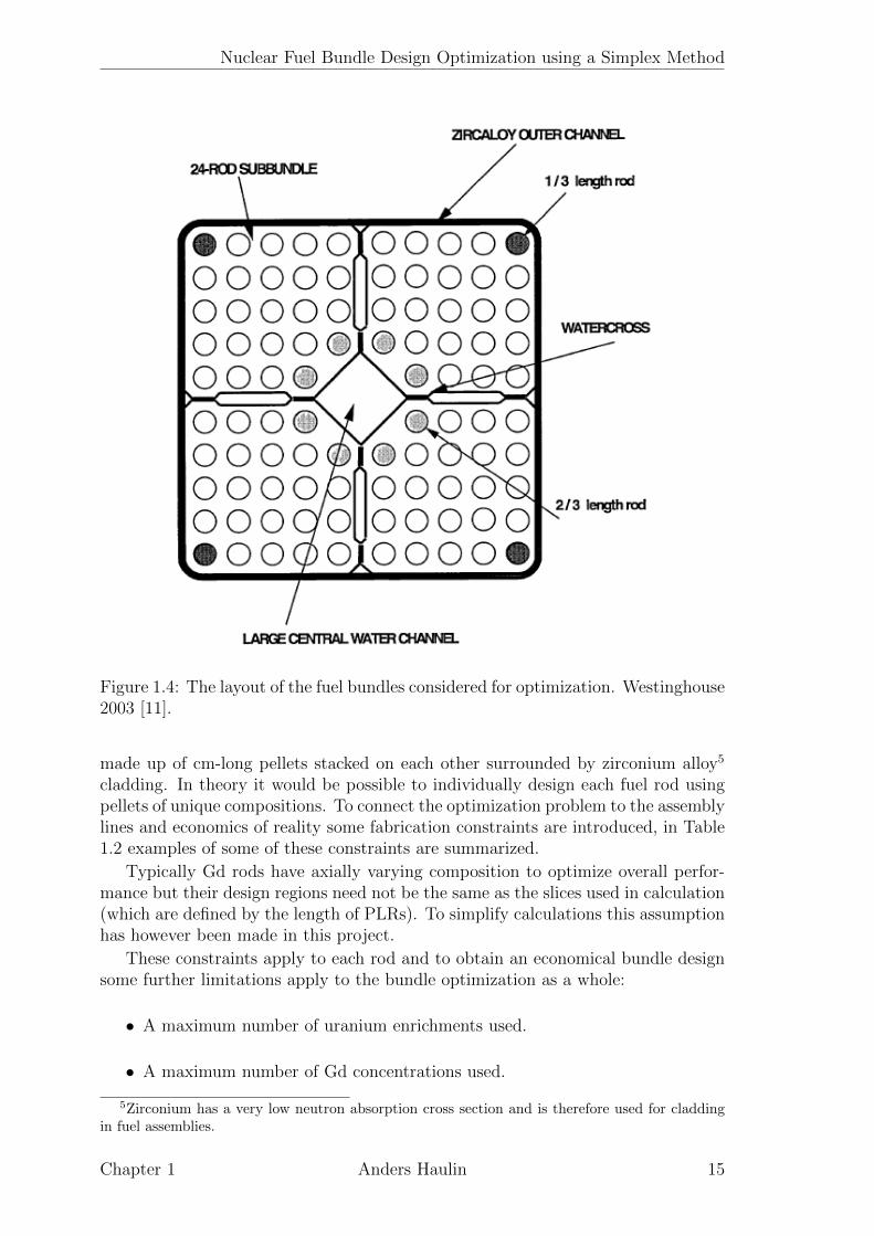
The BWR bundles considered for optimization are made up of 10x10 grids with awater cross of four central non-fuel positions for a total of 96 fuel rods. The bundleis considered to consist of four sub-bundles (NW, NE, SE, SW) of 24 rods each;within a sub-bundle rod spacing is almost equal, whereas the rod to rod distancesbetween neighboring sub-bundles are somewhat greater due to the presence of thewater cross. A special feature of the assembly designs considered for optimizationis that they contain partial length rods, these are rods of approximately 1/3 or 2/3the length of the fuel assembly. These rods are located in the center and corners of
Chapter 1 Anders Haulin 13
Nuclear Fuel Bundle Design Optimization using a Simplex Method
0 10 20 30 40 50 60 70 800.7
0.8
0.9
1
1.1
1.2
1.3
1.4
1.5
k∞
profile of a fuel bundle segment without (blue) and with (green) BA
Bundle burnup (GWd/tU)
k∞
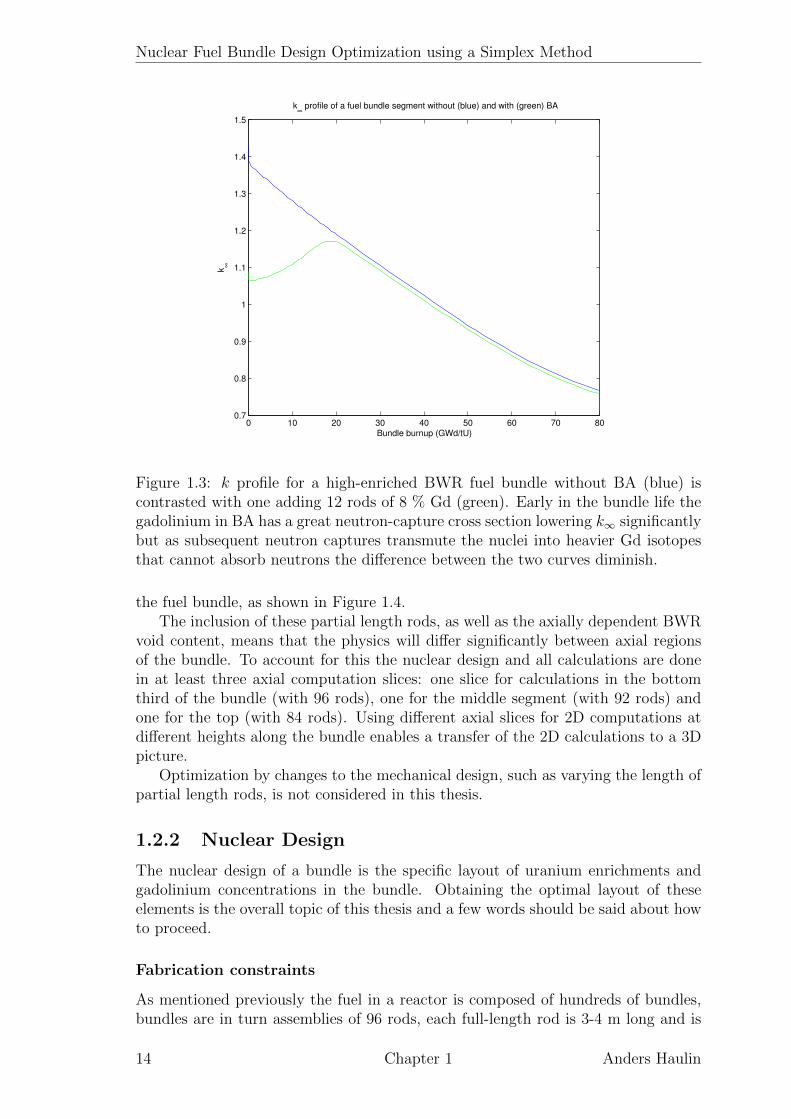
Figure 1.3: k profile for a high-enriched BWR fuel bundle without BA (blue) iscontrasted with one adding 12 rods of 8 % Gd (green). Early in the bundle life thegadolinium in BA has a great neutron-capture cross section lowering k∞ significantlybut as subsequent neutron captures transmute the nuclei into heavier Gd isotopesthat cannot absorb neutrons the difference between the two curves diminish.
the fuel bundle, as shown in Figure 1.4.The inclusion of these partial length rods, as well as the axially dependent BWR
void content, means that the physics will differ significantly between axial regionsof the bundle. To account for this the nuclear design and all calculations are donein at least three axial computation slices: one slice for calculations in the bottomthird of the bundle (with 96 rods), one for the middle segment (with 92 rods) andone for the top (with 84 rods). Using different axial slices for 2D computations atdifferent heights along the bundle enables a transfer of the 2D calculations to a 3Dpicture.
Optimization by changes to the mechanical design, such as varying the length ofpartial length rods, is not considered in this thesis.
1.2.2 Nuclear Design
The nuclear design of a bundle is the specific layout of uranium enrichments andgadolinium concentrations in the bundle. Obtaining the optimal layout of theseelements is the overall topic of this thesis and a few words should be said about howto proceed.
Fabrication constraints
As mentioned previously the fuel in a reactor is composed of hundreds of bundles,bundles are in turn assemblies of 96 rods, each full-length rod is 3-4 m long and is
14 Chapter 1 Anders Haulin
Nuclear Fuel Bundle Design Optimization using a Simplex Method
Figure 1.4: The layout of the fuel bundles considered for optimization. Westinghouse2003 [11].
made up of cm-long pellets stacked on each other surrounded by zirconium alloy5
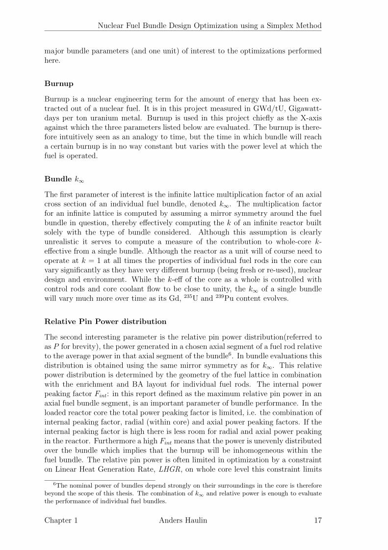
cladding. In theory it would be possible to individually design each fuel rod usingpellets of unique compositions. To connect the optimization problem to the assemblylines and economics of reality some fabrication constraints are introduced, in Table1.2 examples of some of these constraints are summarized.
Typically Gd rods have axially varying composition to optimize overall perfor-mance but their design regions need not be the same as the slices used in calculation(which are defined by the length of PLRs). To simplify calculations this assumptionhas however been made in this project.
These constraints apply to each rod and to obtain an economical bundle designsome further limitations apply to the bundle optimization as a whole:
• A maximum number of uranium enrichments used.
• A maximum number of Gd concentrations used.
5Zirconium has a very low neutron absorption cross section and is therefore used for claddingin fuel assemblies.
Chapter 1 Anders Haulin 15
Nuclear Fuel Bundle Design Optimization using a Simplex Method
Rod types Axial distribution Possible concentrationsUranium rods Entire rod homogenous 2.4 - 4.8% w/o U235 in 0.2%
increments and 4.95%.BA rods 3 axial zones (bottom, mid-
dle, top), with individualGd & U properties
0% and 2 to 8% Gd in 0.5%increments. Enrichments asfor pure uranium rods.
Table 1.2: Examples of fabrication constraints used in optimization.
• A maximum number of Gd rod types, a rod design with a specific U and Gdprofile.
Optimization goals
Apart from generating the best possible bundle performance an optimization mayalso be targeted at reducing the complexity and cost of the manufacturing by tar-geting the number of fuel rod types used or the total number of Gd rods.
2 2 3.4 3.4 2.8 2.8 3.4 3.4 2.8 2
2 3.2 & 3 % 4.4 4.4 3.8 3.8 4.4 4.4 3.2 & 3 % 2.8
3.4 4.4 4.4 4.4 3.4 3.4 4.4 4.4 4.4 3.4
3.4 4.4 4.4 3.2 & 3 % 3.8 3.8 3.2 & 3 % 4.4 4.4 3.4
2.8 3.8 3.4 3.8 3.8 3.4 3.8 2.8
2.8 3.8 3.4 3.8 3.8 3.4 3.8 2.8
3.4 4.4 4.4 3.2 & 3 % 3.8 3.8 3.2 & 3 % 4.4 4.4 3.4
3.4 4.4 4.4 4.4 3.4 3.4 4.4 4.4 4.4 3.4
2.8 3.2 & 3 % 4.4 4.4 3.8 3.8 4.4 4.4 3.2 & 3 % 2.8
2 2.8 3.4 3.4 2.8 2.8 3.4 3.4 2.8 2
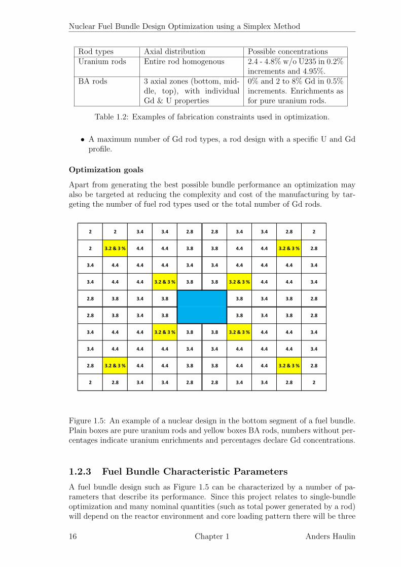
Figure 1.5: An example of a nuclear design in the bottom segment of a fuel bundle.Plain boxes are pure uranium rods and yellow boxes BA rods, numbers without per-centages indicate uranium enrichments and percentages declare Gd concentrations.
1.2.3 Fuel Bundle Characteristic Parameters
A fuel bundle design such as Figure 1.5 can be characterized by a number of pa-rameters that describe its performance. Since this project relates to single-bundleoptimization and many nominal quantities (such as total power generated by a rod)will depend on the reactor environment and core loading pattern there will be three
16 Chapter 1 Anders Haulin
Nuclear Fuel Bundle Design Optimization using a Simplex Method
major bundle parameters (and one unit) of interest to the optimizations performedhere.
Burnup
Burnup is a nuclear engineering term for the amount of energy that has been ex-tracted out of a nuclear fuel. It is in this project measured in GWd/tU, Gigawatt-days per ton uranium metal. Burnup is used in this project chiefly as the X-axisagainst which the three parameters listed below are evaluated. The burnup is there-fore intuitively seen as an analogy to time, but the time in which bundle will reacha certain burnup is in no way constant but varies with the power level at which thefuel is operated.
Bundle k∞
The first parameter of interest is the infinite lattice multiplication factor of an axialcross section of an individual fuel bundle, denoted k∞. The multiplication factorfor an infinite lattice is computed by assuming a mirror symmetry around the fuelbundle in question, thereby effectively computing the k of an infinite reactor builtsolely with the type of bundle considered. Although this assumption is clearlyunrealistic it serves to compute a measure of the contribution to whole-core k-effective from a single bundle. Although the reactor as a unit will of course need tooperate at k = 1 at all times the properties of individual fuel rods in the core canvary significantly as they have very different burnup (being fresh or re-used), nucleardesign and environment. While the k-eff of the core as a whole is controlled withcontrol rods and core coolant flow to be close to unity, the k∞ of a single bundlewill vary much more over time as its Gd, 235U and 239Pu content evolves.
Relative Pin Power distribution
The second interesting parameter is the relative pin power distribution(referred toas P for brevity), the power generated in a chosen axial segment of a fuel rod relativeto the average power in that axial segment of the bundle6. In bundle evaluations thisdistribution is obtained using the same mirror symmetry as for k∞. This relativepower distribution is determined by the geometry of the fuel lattice in combinationwith the enrichment and BA layout for individual fuel rods. The internal powerpeaking factor Fint: in this report defined as the maximum relative pin power in anaxial fuel bundle segment, is an important parameter of bundle performance. In theloaded reactor core the total power peaking factor is limited, i.e. the combination ofinternal peaking factor, radial (within core) and axial power peaking factors. If theinternal peaking factor is high there is less room for radial and axial power peakingin the reactor. Furthermore a high Fint means that the power is unevenly distributedover the bundle which implies that the burnup will be inhomogeneous within thefuel bundle. The relative pin power is often limited in optimization by a constrainton Linear Heat Generation Rate, LHGR, on whole core level this constraint limits
6The nominal power of bundles depend strongly on their surroundings in the core is thereforebeyond the scope of this thesis. The combination of k∞ and relative power is enough to evaluatethe performance of individual fuel bundles.
Chapter 1 Anders Haulin 17

Nuclear Fuel Bundle Design Optimization using a Simplex Method
the nominal power in watts per meter of fuel rod but in bundle level optimizationthis value can not be computed and the limit is instead simplified as one on Fint.
R-factor
One important limitation for the core loading is the margin to dryout expressed asCritical Power Ratio (CPR, explained in Section 1.1.4). CPR is calculated usinga correlation where important parameters are bundle power, axial power shape,bundle coolant flow and inlet sub-cooling. The inherent property of the fuel isdescribed by the R-factor (sometimes called K-factor) and is used as input to thecorrelation. The R-factor correlates relative pin power distribution to a measureof dryout sensitivity for the fuel bundle7. Keeping the R-factor low8 will make itpossible to operate the fuel bundle at a higher power level or with a lower coolantflow which has an economical value. Alternatively better CPR performance canbe used for more operational flexibility. The importance of the R-factor on criticalpower ratio is significant: a rule of thumb is that an increase in R-factor of 1 %worsens the CPR by ∼2%[12] but the effect can be even greater [13]9. The R-factor algorithm combines the internal power distribution with the individual fuelrod dryout sensitivities, normally expressed as additive constants. The additiveconstants for a BWR mechanical bundle design are obtained through extensive testsin laboratories where fuel bundles are heated electrically in a manner that simulatesfission heat generation. By conducting experiments with different internal powerdistributions and fitting the results into to a basic theoretical dryout correlation theindividual fuel rod dryout sensitivities are obtained as additive (fitting) constants.The exact components of such a correlation are specific for every fuel vendor andmodel but the main equations are similar; the correlation studied in this thesisis based on XL boiling length correlation[13]. The basic formula for the R-factorcalculation is common for most XL correlations and here it is given in a generalform without weighting factors or additive constants, Equation 1.4.
Ri,s,z =
(T
Sz
)1/2[WIi · (ri,s,z)1/2 + SJi,s,z + SKi,s,z
WIi +∑nj
j=1 WJj +∑nk
k=1 WKk
]+ Ii (1.4)
T , Sz, WIi, WJj and WKk are weight factors dependent on bundle mechanical andri,s,z is a function of the power in a relative to its sub-bundle, Equation 1.5.
ri,s,z =Pi,s,z · Sz
Ps,z
(1.5)
7An example of R-factor effects: assuming the bundle in Figure 1.4 has a homogeneous powerdistribution it will have a much greater margin to critical heat flux in the corner rods since thesehave much greater contact with water than the internal rods, the R-factor is therefore used toquantify the effects of bundle power distribution and geometry on core CPR performance.
8Specifically keeping the maximum R-factor of the bundle low. The rod with the highest R-factor is said to be R-limiting and minimizing bundle maximum R-factor is a common optimizationobjective.
9Page 298.
18 Chapter 1 Anders Haulin

Nuclear Fuel Bundle Design Optimization using a Simplex Method
SJ , SK are non-linear functions using the smallest value of nodal power in pin iand a weighted average of side 1.6 or diagonally 1.7 bordering nodal powers.
SJi,s,z = min
(nj∑j=1
WJj · (rj,s,z)1/2, (ri,s,z)1/2 ·
nj∑j=1
WJj
)(1.6)
SKi,s,z = min
(nk∑k=1
Wkk · (rk,s,z)1/2, (ri,s,z)1/2 ·
nk∑k=1
Wkk
)(1.7)
It should be observed that there are two major non-linearities here, the square-rootdependence on fuel rod power and the two functions of minima. In a linearizationscheme this must be accounted for in some fashion, this will be further investigatedin the results, Chapter 5.
1.3 The case for automatic optimization
The design process for a BWR fuel bundle is part of the greater reactor reload designprocess where several types of new fuel bundles are engineered and combined withre-used bundles in a core-loading pattern for maximum plant performance. To cre-ate the nuclear design of uranium enrichments and BA concentrations in a bundle,nuclear engineers will typically go through a process based on previous experienceas well as trial-and-error. From specifications on k∞-profile they can deduce a roughmeasure of average bundle enrichment, number of BA rods and Gd concentration.From this estimate they will then choose different rod patterns and evaluate them(of great interest are their R and Fint profiles) until arriving at a bundle design withthe desired attributes and characteristic parameters. It is this bundle-level processthat this project has sought to automate by simplex optimization. Automatic opti-mization has been a topic of research in nuclear engineering for a long time. Whilewhole-core level optimization has been a well investigated territory[14], the aspectof optimizing the design of a single fuel bundle is less well documented10.
1.3.1 The problem at hand
The task of designing a nuclear fuel bundle is intuitively well suited for automaticoptimization: the problem is simply to assign values at every point in a grid in amanner such that one obtains the best possible evaluation of a specified objectivefunction. The design constraints mentioned in the design section imply that a typicaldesign containing 18 Gd rods with three axial slices has 78 uranium rods and 54individual BA rod segments to optimize (BA nodes will be assigned both a Gdconcentration and a uranium enrichment). The fabrication constraints adopted, 14permitted enrichments and 16 gadolinium concentrations (including 0%) gives over
n =
(96
18
)· 1478 · (14 · 16)54 (1.8)
10A possible exception to this is the N-streaming concept[15] which approaches the loadingpattern and bundle design problem of a BWR by repeatedly targeting the worst rod in the worstbundle according to some optimization target. The details of this approach are not well documented(publicly) and the method may not be considered to be a true optimization algorithm.
Chapter 1 Anders Haulin 19

Nuclear Fuel Bundle Design Optimization using a Simplex Method
or 10235 possible layouts. In reality the vast majority of the combinations in Equa-tion 1.8 are easily excluded for a number of reasons. For an isolated fuel bundlethere would be no point in breaking symmetry in the design: a skewed layout willexhibit skewed suboptimal power distributions and utilize neutrons inefficiently. Ifthe environment surrounding the quadratic bundle is homogeneous it would indeedsuffice to examine an eighth of the bundle. However, the environment in the reactoris not homogeneous because of the presence of control rods: in this project these areviewed as blades covering two of the sides in a (for example the North and West side)which generates a diagonal symmetry. This reduces the 10x10 grid to 55 positionsof which 52 are occupied by fuel rods.
After including more realistic fabrication constraints such as:
• Total of 6 enrichments used.
• Total of 2 Gd concentrations used.
• Three types of BA rods, with axial specific Gd and U profiles.
• No BA in peripheral positions of the bundles and in partial length rods.
and assuming 10 are Gd rods with two of these on the symmetry line the numberof combinations is reduced to:
n =
(29
10
)·(
10
3
)· (123 · (122 · 6)2) · 642 ·
(14
6
)·(
15
2
)(1.9)
or 5 · 1056 combinations. The majority of these designs will be incompatiblewith average enrichment targets and the like, but it still remains a magnificent-sizedproblem.
The overwhelming issue with optimizing this grid is that the values of interest;such as the internal form factor Fint and k∞, depend on the layout in a highlynon-trivial manner. A simple function for the exact dependence of the form factoron enrichment or Gd concentration cannot simply be constructed. Without ananalytic function from input to output we cannot obtain an analytic gradient, andoptimization strategies based on those are therefore useless. In this project thecalculations of the bundle parameters have been conducted by a licensed 2D coarse-grid finite mesh program, PHOENIX (referred to as 2D lattice code), that putsup neutron balance equations and solves them using vast cross section libraries toobtain power distributions and k∞ as a function of burnup. Using this program ithas during the project been possible to calculate around 10 slice designs in parallelwith approximately 10 seconds computing time on the cluster (during normal use).It is therefore evident that simply evaluating any significant fraction of the possibledesigns without a clever strategy is impossible in decent time.
1.3.2 Optimization strategies
Without an analytic gradient to work with the scope for optimization appears ratherlimited. There are however techniques that can approach a problem such as this.These techniques can generally be divided into deterministic and stochastic methods.
20 Chapter 1 Anders Haulin

Nuclear Fuel Bundle Design Optimization using a Simplex Method
Stochastic methods
Stochastic methods utilize random but clever perturbations with inspiration fromevolutionary biology’s natural selection11 or condensed matter physics’ annealingprocesses12 to generate the bundle designs to evaluate. The greatest strengths ofstochastic algorithms is that the evaluation part can be done in any way with anytype software being chosen and that the objective function can use any result fromthis evaluation13. A weakness is however that fuel bundle PHOENIX evaluationshave to be done for every considered design in every step and that the program willmore or less run blindly. It will not know whether the objective function value beingsought is unobtainable or how long calculation time a successful optimization willtake [19]. It is also vulnerable to local optima, a perturbation contribution (muta-tions in the GA example) ensures some departure from local optima but there is noguarantee that the best possible solution was not a combination of two “inferior”parents that were both discarded on their individual merit [14].
Deterministic methods
To avoid these pitfalls of stochastic optimization this project uses a deterministicmethod, namely the simplex method. This method is a linearization scheme thatcan optimize any linear problem. Although less exact in each evaluation, it hasthe great advantage of giving the user the power to choose the balance betweenoptimality and calculation time.
1.3.3 The simplex method
The simplex model is a widely used deteministic optimization method; commercialsimplex programs include CPLEX (used in this thesis) and Gurobi (a potential al-ternative). It has several advantages over stochastic methods in that it does notget trapped in local optima, can quickly determine whether a set of constraints isinfeasible and can give an approximation of how close to the global optimum a foundsolution is. Its key disadvantage is that its assumption of linearity along with thenon-linearity of the real world necessitates several linearizations of the problem athand. The degree of success of using the simplex model on this problem will dependon the validity of the model being used: if large errors propagate in the optimizationprogram’s approximations then the task of finding the design which performs bestaccording to these approximations becomes pointless as its connection to reality issevered. A key task in this thesis has therefore been to evaluate the approxima-tions used in the program and if possible improve them. Better approximations
11Called genetic algorithms, GA.12Simulated Annealing or SA.13A genetic algorithm applied on a fuel bundle optimization problem would widely follow these
few steps, words in italic are biology parallels: 1. Stochastically generate a large number of bundledesigns, a population. 2. Convert the bundle design to a string of values, a genome. 3.Evaluate thedesigns and calculate their respective fitness values according to an objective function. 4.Discardthe worst X percent of the population, survival of the fittest. 5.Stochastically combine genomesof the survivors, breeding. 6.Impose some random mutations on the property strings. 7.Return toevaluation stage with the new generation of designs. After a set number of times or when a desiredobjective function value is reached, the program can terminate and the best design be presented.
Chapter 1 Anders Haulin 21
Nuclear Fuel Bundle Design Optimization using a Simplex Method
are likely to increase the size or complexity of the problem, thereby prolonging theoptimization run-time.
1.3.4 Other work in the field
The simplex method has been implemented previously for whole-core loading patternoptimization, for example by Kim & Kim [17]. In their model core-reactivity istargeted for maximization at end-of-cycle. Including other optimization methodsthere are several patents regarding whole-core nuclear optimization ([19],[18]), butno patents solely pertaining optimization of individual bundles have been found.
22 Chapter 1 Anders Haulin
Chapter 2
Existing Optimization Strategy
2.1 Outline
The tool used to improve upon in this thesis is a framework of programs operatingin the following manner:
• Reference nuclear designs are entered and many new designs with grid posi-tions individually perturbed in enrichment or BA are generated from them.
• Perturbed designs are sent to a 2D lattice code running on a cluster to performcalculations.
• Result data is extracted from files to form sensitivity matrices for use in acommercial simplex program (CPLEX).
• Sensitivity matrices for different bundle parameters enter into an optimiza-tion module in a commercial simplex program for optimization of BA andenrichments.
• Simplex optimizer evaluates designs and outputs the values of decision vari-ables which, in its approximated model, correspond to the optimal design.
The optimization code written in proprietary Optimization Programming Language(OPL) implemented on IBM’s CPLEX optimizer. The idea behind this strategyis that the effect of a number of combined perturbations can be reasonably wellapproximated by the sum of their individual contributions to any fuel parameter.The optimization strategy used is extremely versatile and it provides an exhaustivesearch of the solution space thanks to simplex implementation. It can not onlyproduce a solution but also compare its objective function to an approximation ofthe objective function of the global optimum.
The framework used in the project optimized the design in two distinct steps: thefirst step took a fixed enrichment distribution reference without BA to optimize BApositions with regard to bundle parameter constraints and optimization objectives,the second step fixed these BA positions to optimize the enrichment in each fuelrod and the Gd concentration in the BA rods. The reason for this division of taskshad been that both approximation errors and computing times became very large inexperiments for this larger more general problem. A more detailed justification forthis approach will be given in Section 5.1.1. The first step had been evaluated in some
23

Nuclear Fuel Bundle Design Optimization using a Simplex Method
detail and measures had been taken to mitigate approximation errors, the secondstep was, however, untested by the intended users (the problems concerning this areexplained in Section 3.2.1). The simplex implementation of the two steps in CPLEXwas slightly different. The perturbation variables for Gd position and concentrationin step 1 were integers taking of dimensions rod number and Gd-concentration, thustaking the value 1 at combinations that were true and 0 where they were false. Thesecond step instead formulated linear decision variables as floats, ∆-enrichment and∆-Gd, the resulting variables for chosen enrichments and Gd concentration were,however, limited to certain allowed values: effectively making these variables binaryas well.
To represent the actual physics in the reactor a large number of constraintsare needed to link the decision variables of enrichment and BA distribution to realparameters such as k∞, the fuel rod relative power distribution, internal powerpeaking factor (Fint) and R-factor. The key limitation using a simplex model is thatthese constraints have to be expressed linearly. In the results section an analysis ofthe linearization errors associated with these approximations is presented.
Linear perturbation terms are computed by running a large number of possibleperturbations in the design through a 2D lattice code obtaining values of the relevantparameters P and k∞. From this, sensitivity matrices (S-matrices) are generated:as an example the enrichment S-matrix element for k∞ perturbation in a certain rodis computed in the following manner.
• A reference design is entered into the 2D lattice code by the user.
• Two designs, where the enrichment in the specific fuel rod is changed to themaximum allowed enrichment and lowest allowed enrichment respectively, areentered by script programs.
• k∞-values are automatically extracted from the 2D lattice code output and thedifference between the maximum and minimum cases is computed and dividedby the enrichment difference.
• The value ∆k∞∆U
is computed and entered into an S-matrix file (in this projectan Excel-file through a macro).
The S-matrix elements for the relative fuel rod power distribution are calculated ina similar way but here S-matrix elements for one perturbed fuel rod position arecalculated for both the specific rod where the perturbation is done and for all otherfuel rod positions in the bundle. For a typical fuel bundle there are 52 rods (takingsymmetry into account) with 3 axial slices (their number can be chosen freely but 3are always used in this project since it is the minimum required to correctly modelpartial length rods) for which perturbations need to be calculated. Computing theS-matrix elements therefore requires 315 simulations for the enrichment alone (a maxmin run for every position, plus three reference runs). Fortunately the core simulatorruns on a cluster and will therefore usually calculate 10-12 cases simultaneously,finishing the entire process in less than 10 minutes. The resulting sensitivity matrixfor k∞ has 52 elements (one for each rod, using symmetry) for every burnup stepconsidered. The parameters R and P are rod-wise properties which mean that therewill be one sensitivity matrix for every axial segment of every fuel rod. Pin powersensitivity matrices take into account every other rod in the same slice which gives
24 Chapter 2 Anders Haulin

Nuclear Fuel Bundle Design Optimization using a Simplex Method
52 · nbu (number of burnup steps) elements in every matrix. R-factor calculationsare done by sub-bundle which means that the size of the S-matrices for R follow thenumber of independent fuel rods in the sub-bundle in question1. These figures areindicators of the size of the problem and explain why these simplex optimizationstypically have around 100000 variables. The S-matrix files are read by the simplexprogram (CPLEX) and the sensitivity matrix elements are implemented as linearprogramming constraints in between “true” decision variables enrichments and Gdconcentration on one hand, and the result decision variables such as k∞ and P 2.
Upon starting the project the actual procedures of generating input for PHOENIXcalculations to create S-matrices and putting them into excel sheets was very cum-bersome, but since the data management is not a focus of this thesis no greatereffort has been made to alter it.
2.2 Constraints and objective
To connect the decision variables used by CPLEX to each other and the constantsdescribing the problem a long list of constraints is needed, the constraints can bedivided into four different classes.
• Constraints representing the approximations for bundle physics parameters.
k∞ = kref∞ +
nU∑i
(∆iU · SUi ) +
nGd∑j
(∆jGd · SGdj ) (2.1)
Meaning that the k∞ value in the bundle is equal to the reference bundlek∞ plus the sum of the changes in Uranium enrichments rodwise multipliedby S-matrix elements plus the sum of changes in Gadolinium concentrationsrodwise multiplied by their S-matrix elements over the BA rods.
• Constraints describing actual constraints on parameters in the model.
max(Pi,z) < Limit (2.2)
• Constraints representing fabrication constraints, such as maximum number ofenrichments utilized.
• Logical constraints, such as ”one and only one enrichment per rod position”,to eliminate bogus solutions.
The distinction between the first two types of constraints if for convenience,they could very well be combined into the same equations but on a problem of thisscale that would make the OPL code much less readable without gaining anythingin optimization time. The objective is the decision variable that CPLEX seeks to
1R-factor calculations do take into account the power of other sub-bundles, but through a scalar“mismatch factor”, therefore there are either 14 (NW&SE) or 24 (SW) S-matrix elements for everyburnup step.
2In the CPLEX implementation, variables such as k∞ and ∆Gd are not fundamentally different;they are both treated as decision variables for CPLEX to assign values to. Through constraintequations using S-matrix values these decision variables are linked by the linear equations formu-lated.
Chapter 2 Anders Haulin 25
Nuclear Fuel Bundle Design Optimization using a Simplex Method
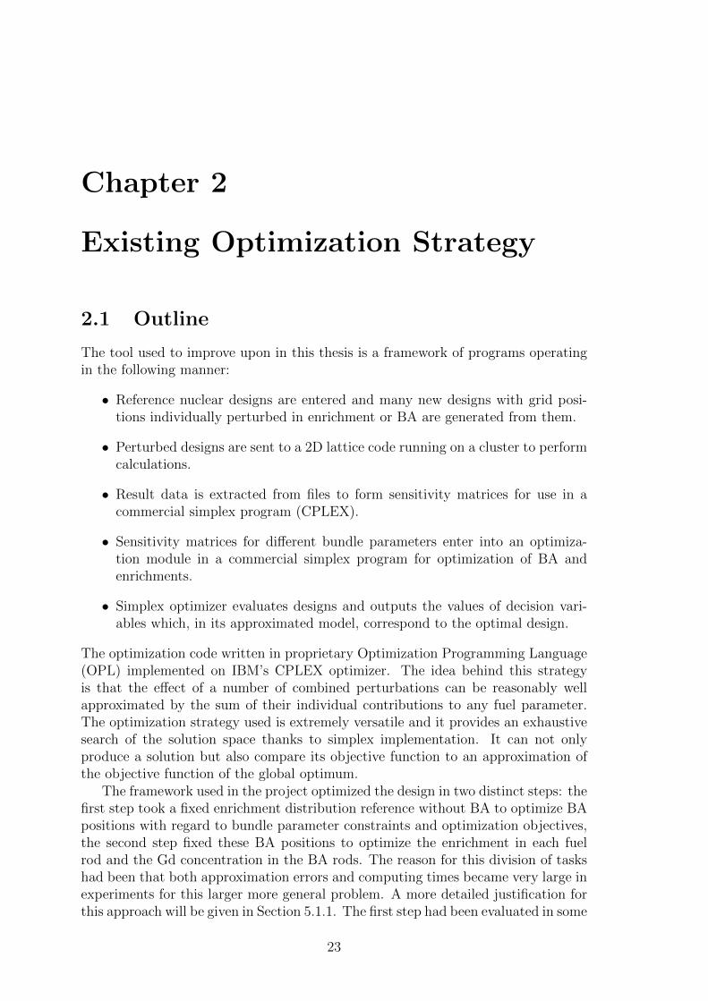
minimize (or maximize), it must be a real scalar but that can in turn for examplebe a sum of several variables or a maximum of a vector in some interval. The mostcommon objective in this project was minimization of the bundle R-factor. A glanceof the CPLEX progress window is seen in Figure 2.1. An optimization following the
Figure 2.1: Part of the CPLEX window showing parameters of a running optimiza-tion and its progress. The user can view the progress of an optimization with itsincumbent solution and an estimated bound of the global optimum, the differencebetween the two is referred to as the gap.
described framework runs in CPLEX until the ratio of the best found objective func-tion value to CPLEX’s estimate of the global best value comes within a prescribed”gap tolerance”3. When the optimization terminates the design associated with thebest objective function value is post-processed and exported, its most importantparameters are of course the enrichment and/or BA profile.
3During a minimization the best found value will decrease as new better designs are found, andthe estimate will increase as more and more branches are evaluated and their actual best valuesare found.
26 Chapter 2 Anders Haulin
Chapter 3
Method
3.1 Research Questions
The project broadly followed the topics of a set of research questions.
• Can a linear approximation of the constitutive relations in a nuclear fuel bundlethrough a simplex optimization generate potential nuclear fuel bundle designs?How does the existing scheme perform and how can it be improved?
– How do the initial conditions of enrichment and BA weights specified inthe reference affect the outcome?
– How do results from such an optimization compare to “manually opti-mized” designs made by nuclear engineers using perturb-and-investigateprograms?
– Is it feasible and motivated to incorporate 2nd order terms, or piecewiselinear approximations in the optimization method (thereby increasing thesize of the simplex problem) and how much would this affect optimizationtime?
– Are there major simplifications that can be made?
• Are there optimization problems associated with reactor cycle length?
• How much engineering time can be saved with a functional optimization tool?Which barriers hinder implementation?
• Does the optimization tool have a value beyond associated time-savings in thedesign phase? Would other parties be interested in applying it?
• Is it possible to reduce the total number of BA rods in a bundle compared tomanually optimized designs?
• Can bundle design optimization be coupled with core-loading pattern opti-mization?
• How should the project proceed?
27

Nuclear Fuel Bundle Design Optimization using a Simplex Method
3.2 Project Progression
The project for this thesis was suggested by a nuclear company with a prototypeBWR Fuel Bundle Design Optimization project. The thesis was supposed to inves-tigate the validity of the designs suggested by the program and compare these withdesigns obtained by nuclear engineers using manual trial-and-error schemes to pro-duce a recommendation for further development of the tool. To pursue the strategyknowledge would have to be gained in the theory and programming of optimization.This was the initial method used but due to the prototype nature of the program atwo-prong strategy was used: optimizations would be run from start to finish whileerror-checking and obtaining a functioning strategy to finally use this strategy torun optimizations on cores where manual designs had already been made. Usingthese as a benchmark the performance of the optimization scheme could then beevaluated, conclusions could be drawn and recommendations formulated.
3.2.1 Practical Issues
Using the prototype optimization framework proved harder than expected for anumber of reasons. Unnecessarily complicated data handling made the system error-prone and although several modifications were made to improve it the focus of theproject was not to produce a production-ready program so most of the programsinvolved were only modified rather than replaced within this thesis project.
During the project it was found that the optimization framework contained someunfinished areas and errors. Some of the issues were:
• Optimization step 1 could functionally optimize BA placements but the en-richment and Gd concentration optimization in step 2 was hard-coded for asingle case of BA placements.
• Symmetries were not fully utilized. In the S-matrix generation full bundle(i.e. without diagonal symmetry) calculations were used. The result of anoff-diagonal perturbation was then expressed as the sum of the response ofthe two symmetric positions in lower left half and the upper right half of thebundle. This way some accuracy is lost for positions close to the symmetrydiagonal since interaction between the perturbed positions makes for non-additive results.
• No functionality to control average enrichment.
• Some errors were present in R factor calculations, including weighting factorsand faulty linearizations.
• k∞ profile in the enrichment optimization step (step 2) could not be determinedbut was instead constrained only so that the starting value from step 1 didnot change. This made it impossible to define a desired k∞ profile while alsomaking the problem artificially seem much smaller than it was.
• Pre- and post-processing features in CPLEX not fully utilized.
• The only initially available CPLEX computer was very slow and its programversion old, making full sequences of optimizations for relevant burnup lengthsnigh-impossible to run.
28 Chapter 3 Anders Haulin
Nuclear Fuel Bundle Design Optimization using a Simplex Method
3.2.2 Improving the Approximations
During the project the main body of work concerned several methods of improvingthe accuracy of the model to evaluate how optimality could be improved. The resultsof these investigations are covered in the results section and they included.
• Piecewise linear approximations of characteristic parameters.
• Adapting input reference cases to match the desired design as much as possible,without loss of generality.
• Quadratic approximations for bundle design parameters.
• Shadow-factor correction for k∞ approximations in step 1 extended to step 2.
• Omitting R-factor calculations entirely, instead replacing them with relativepin power targets.
3.3 Two Optimization Cases
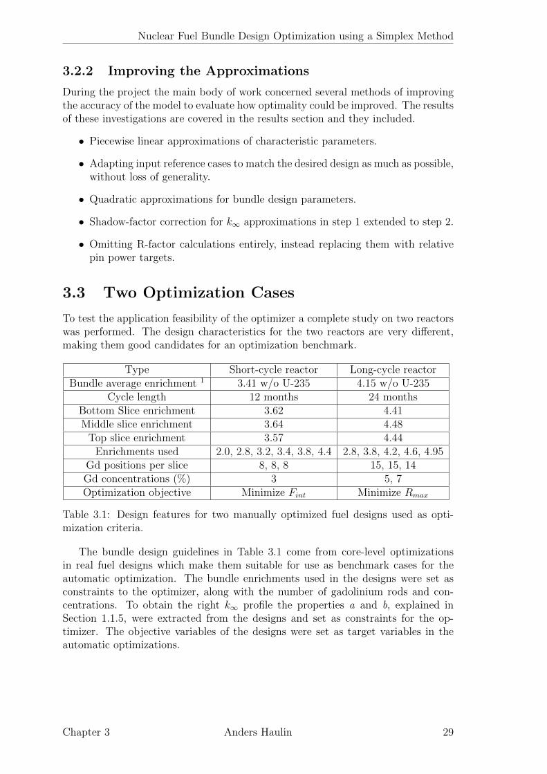
To test the application feasibility of the optimizer a complete study on two reactorswas performed. The design characteristics for the two reactors are very different,making them good candidates for an optimization benchmark.
Type Short-cycle reactor Long-cycle reactorBundle average enrichment 1 3.41 w/o U-235 4.15 w/o U-235
Cycle length 12 months 24 monthsBottom Slice enrichment 3.62 4.41Middle slice enrichment 3.64 4.48
Top slice enrichment 3.57 4.44Enrichments used 2.0, 2.8, 3.2, 3.4, 3.8, 4.4 2.8, 3.8, 4.2, 4.6, 4.95
Gd positions per slice 8, 8, 8 15, 15, 14Gd concentrations (%) 3 5, 7Optimization objective Minimize Fint Minimize Rmax
Table 3.1: Design features for two manually optimized fuel designs used as opti-mization criteria.
The bundle design guidelines in Table 3.1 come from core-level optimizationsin real fuel designs which make them suitable for use as benchmark cases for theautomatic optimization. The bundle enrichments used in the designs were set asconstraints to the optimizer, along with the number of gadolinium rods and con-centrations. To obtain the right k∞ profile the properties a and b, explained inSection 1.1.5, were extracted from the designs and set as constraints for the op-timizer. The objective variables of the designs were set as target variables in theautomatic optimizations.
Chapter 3 Anders Haulin 29
Chapter 4
Apparatus
4.1 S-matrix hardware and software
4.1.1 Hardware
The nuclear calculations for bundle parameters were done on a local UNIX cluster,generally it allocated 10 or more cores to the perturbation computations necessaryfor S-matrix generation.
4.1.2 Software
Apart from the licensed 2D lattice code PHOENIX a number of other programs wereused on the cluster: a local program that took 2D pin powers to calculate R-factorsas well as MATLAB for simulations of R-factor behavior and enrichment inputs.The output files from the simulator were read and S-matrix elements calculated bylocally developed FORTRAN scripts, which were eventually re-written. The outputfiles from these scripts were later exported into Excel file format using Excel macros,these Excel files could in turn be read by CPLEX for optimization input.
4.2 Simplex optimization hardware and software
4.2.1 Hardware
Initially the CPLEX optimizations were run remotely over the Atlantic on a 10 yearold desktop computer with a 2 GHz dual-core Intel processor and 2GB RAM.
At the end of the project a new remotely operated computer was installed, thismachine had two processors with 4 dual-thread 2.4 GHz processors each for a totalof 16 CPLEX threads on 32 GB RAM.
4.2.2 Software
The proprietary simplex optimization suite CPLEX was used throughout the project.CPLEX is an IBM program with an associated proprietary optimization program-ming language OPL. The codes available at the start of the project were written inOPL and executed in CPLEX 12.2.
30
Nuclear Fuel Bundle Design Optimization using a Simplex Method
4.2.3 Equipment upgrade
Along with the new hardware that became available late in the project a newerversion (12.6) of CPLEX was installed: this version had improved heuristics andwhen supplied the same problem as the old one it reported a different size of theresultant matrix. The impact from upgrading hardware and software was immedi-ate and positive bordering on painful. The computation time needed to find onepossible solution (although not the optimal by far) for an enrichment optimizationproblem decreased from 17 hours to 4 minutes. Before this upgrade it had notbeen possible, using the available framework, to run optimizations on long enoughburnup intervals and experiments were limited to investigation of approximationsrather than comparisons to manual designs. After the new machine was installed itbecame possible to optimize enrichments for adequately long burnup intervals andto consider any extensions of the project calculating parameters more efficiently.
Chapter 4 Anders Haulin 31
Chapter 5
Results
5.1 Evaluating the framework
A considerable part of the project concerned the evaluation of the framework previ-ously developed described in chapter 2 and specifically the effects of the linearizationemployed in the optimization. This had not before been well investigated and a re-view was necessary to improve the framework.
5.1.1 Two-step approach
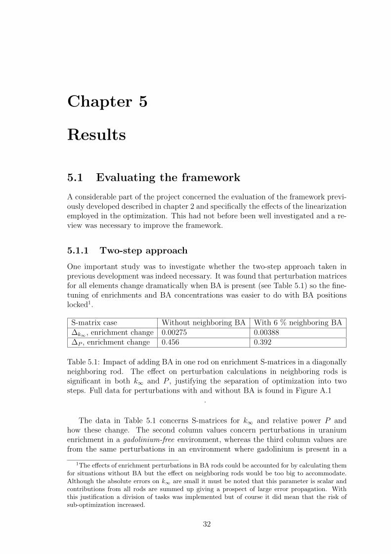
One important study was to investigate whether the two-step approach taken inprevious development was indeed necessary. It was found that perturbation matricesfor all elements change dramatically when BA is present (see Table 5.1) so the fine-tuning of enrichments and BA concentrations was easier to do with BA positionslocked1.
S-matrix case Without neighboring BA With 6 % neighboring BA∆k∞ , enrichment change 0.00275 0.00388∆P , enrichment change 0.456 0.392
Table 5.1: Impact of adding BA in one rod on enrichment S-matrices in a diagonallyneighboring rod. The effect on perturbation calculations in neighboring rods issignificant in both k∞ and P , justifying the separation of optimization into twosteps. Full data for perturbations with and without BA is found in Figure A.1
.
The data in Table 5.1 concerns S-matrices for k∞ and relative power P andhow these change. The second column values concern perturbations in uraniumenrichment in a gadolinium-free environment, whereas the third column values arefrom the same perturbations in an environment where gadolinium is present in a
1The effects of enrichment perturbations in BA rods could be accounted for by calculating themfor situations without BA but the effect on neighboring rods would be too big to accommodate.Although the absolute errors on k∞ are small it must be noted that this parameter is scalar andcontributions from all rods are summed up giving a prospect of large error propagation. Withthis justification a division of tasks was implemented but of course it did mean that the risk ofsub-optimization increased.
32

Nuclear Fuel Bundle Design Optimization using a Simplex Method
neighboring rod. It is clear that the introduction of gadolinium changes the S-matrix elements for enrichment perturbations quite substantially, and this warrantsthe division of tasks used in the optimization: where BA placements are handledby themselves so as to not affect the accuracy of calculations concerning enrichmentvariations.
Second step issues
As aforementioned the second CPLEX optimization step concerning enrichmentsand Gd concentrations had not previously been well-tested and a substantial effort(re-writing a few hundred lines of code) had to be made to generalize the datahandling and constraints since these had been hard-coded for a reference case with acertain set of BA rod types and positions. Introducing variables for BA rod types andpositions required some work but did neither change the result nor the execution ofthe hard-coded reference case, therefore full optimizations could continue for any BAgeometry using the re-written code representing the same fundamental equations.Something that did change the computation time was a change in how the k∞ profilein the second step was limited, the code received at the onset of the project limitedk∞ at 0 burnup to within a very small (100 pcm) interval around that of the referencedesign, which basically prohibited the second step from doing any major changes tothe design as these would violate this condition. This criterion did not reflect thenuclear design process and was instead replaced by criteria on two parameters: thedifference in k∞ at 0 GWd/tU burnup which would result from removing all BA inthe design, called a, and the burnup at which maximum bundle k∞ occurs, called b.These values, along with the average enrichment, are required to fully constrain thek∞ of the bundle and were therefore approximated in the simplex model. Rewritingthe program so that k∞ followed conditions on the a and b parameters meant thatmany more designs became possible and the calculation time increased by more thanone order of magnitude.
5.1.2 Symmetry issues
The existing optimization model uses diagonal symmetry, as described in the theorysection. However, the perturbation matrices were generated with full-bundle cal-culations making perturbations only in the lower-left half. The results from theseperturbations in the lower and upper half was added, i.e. the S-matrix value fora change in rod position (I,J) is set to the sum of the result in positions (I,J) and(J,I). For k∞ which does not have a position dependence the consequence will bethat the results of a perturbation will simply be doubled to account for the effecton the upper half.
The hypothesis in this project was that this was an unnecessary simplification;actually making the calculation process more cumbersome and less accurate.
Consider first Gd perturbation in rod position (9,2): an assumption of symmetry(maintained throughout this project and justified in the Section 1.3.1) means thatthe same perturbation should be present in (2,9). These rods are far apart from eachother and their interaction can be assumed to be small. However, consider instead aperturbation at (3,2), implying the same perturbation in (2,3): these two rods bordereach other diagonally and it should be expected that the drop in neutron flux and itseffect on k∞ from these two changes will not be twice that of an individual change.
Chapter 5 Anders Haulin 33
Nuclear Fuel Bundle Design Optimization using a Simplex Method
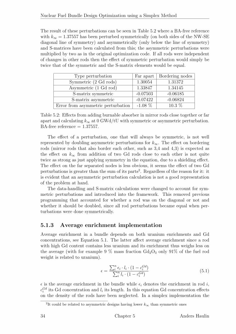
The result of these perturbations can be seen in Table 5.2 where a BA-free referencewith k∞ = 1.37557 has been perturbed symmetrically (on both sides of the NW-SEdiagonal line of symmetry) and asymmetrically (only below the line of symmetry)and S-matrices have been calculated from this; the asymmetric perturbations weremultiplied by two as in the original optimization code. If all rods were independentof changes in other rods then the effect of symmetric perturbation would simply betwice that of the symmetric and the S-matrix elements would be equal.
Type perturbation Far apart Bordering nodesSymmetric (2 Gd rods) 1.30054 1.31372Asymmetric (1 Gd rod) 1.33847 1.34145
S-matrix symmetric -0.07503 -0.06185S-matrix asymmetric -0.07422 -0.06824
Error from asymmetric perturbation -1.08 % 10.3 %
Table 5.2: Effects from adding burnable absorber in mirror rods close together or farapart and calculating k∞ at 0 GWd/tU with symmetric or asymmetric perturbation.BA-free reference = 1.37557.
The effect of a perturbation, one that will always be symmetric, is not wellrepresented by doubling asymmetric perturbations for k∞. The effect on borderingrods (mirror rods that also border each other, such as 3,4 and 4,3) is expected asthe effect on k∞ from addition of two Gd rods close to each other is not quitetwice as strong as just applying symmetry in the equation, due to a shielding effect.The effect on the far separated nodes is less obvious, it seems the effect of two Gdperturbations is greater than the sum of its parts2. Regardless of the reason for it: itis evident that an asymmetric perturbation calculation is not a good representationof the problem at hand.
The data-handling and S-matrix calculations were changed to account for sym-metric perturbations and introduced into the framework. This removed previousprogramming that accounted for whether a rod was on the diagonal or not andwhether it should be doubled, since all rod perturbations became equal when per-turbations were done symmetrically.
5.1.3 Average enrichment implementation
Average enrichment in a bundle depends on both uranium enrichments and Gdconcentrations, see Equation 5.1. The latter affect average enrichment since a rodwith high Gd content contains less uranium and its enrichment thus weighs less onthe average (with for example 9 % mass fraction Gd2O3 only 91% of the fuel rodweight is related to uranium).
ε =
∑ni εi · li · (1− cGd
i )∑ni li · (1− cGd
i )(5.1)
ε is the average enrichment in the bundle while εi denotes the enrichment in rod i,cGdi its Gd concentration and li its length. In this equation Gd concentration effects
on the density of the rods have been neglected. In a simplex implementation the
2It could be related to asymmetric designs having lower k∞ than symmetric ones
34 Chapter 5 Anders Haulin
Nuclear Fuel Bundle Design Optimization using a Simplex Method
average enrichment should be present as a constraint on the problem; this can bevisualized by defining a decision variable depending on enrichment and Gd concen-tration and limiting this to be within a tolerance interval of deviation around thedesired enrichment. Since this equation is not linear it has to be modified to be ableto implement in a simplex optimizer, in this project the easiest route was taken:simply using the reference Gd concentration in the denominator omitting the de-pendence on changes in BA content, thus the problem of dividing decision variableswith each other was eliminated and a linear implementation obtained3.
5.2 Improving approximations
The lion’s share of the project was devoted to improvement of the approximationsand methods used in the optimizer to account for the characteristic bundle param-eters. Given the constraints imposed by linearity two main types of errors wereexpected to be encountered: local non-linearities, that the effect of changing a pa-rameter in a fuel rod segment was not linear, and cluster effects, that the effectof several changes was not equal to the sum of its parts. The tools available tothe simplex program at first seemed limited and two ”strategies” were considered:looping the optimization4 and improving the framework and approximations.
Looping
Looping the optimization is a very crude way of improving results. It entails runningan optimization with low tolerance, accepting the solution as a reference, calculatingnew perturbation matrices and running the optimization again. This can be repeatedas many times as necessary until the discrepancy between PHOENIX results andmodel results diminishes below an accepted value. A major risk is that this partitionleads to sub-optimization by locking on to a poor path. In reality the only increasein accuracy from repeating the optimization will come from the smaller absolutechanges done in the CPLEX step. It was found that the main gain from runningan optimization twice was that the second run can be done without the result andreference average enrichments and gadolinium levels differing very much, that theinitial guess becomes ”better”. This can, however, be done much more easily beforethe first step even starts, see Section 5.2.1. Any repetition of the framework wastherefore discarded, especially considering that the CPLEX run-times were oftenmeasured in hours.
5.2.1 k∞
The most thoroughly examined fuel design parameter was k∞. Due to its scalarnature that takes contributions from an entire slice into account it is more easilygraphed than the fuel rod properties R-factor and relative pin power.
The effects on k∞ from uranium and BA changes are quite different in nature;Figure 5.1 shows the bundle k∞ as a function of varying uranium enrichment in one
3It was late in the project suggested that accounting for BA effects on average enrichmentcould be omitted altogether and possibly speed up optimization, this was not done to keep resultscomparable.
4This was not a very clever or promising strategy, but was investigated nonetheless.
Chapter 5 Anders Haulin 35

Nuclear Fuel Bundle Design Optimization using a Simplex Method
2 2.5 3 3.5 4 4.5 50.903
0.9035
0.904
0.9045
0.905
0.9055
0.906
0.9065
0.907
0.9075
k∞
Pin enrichment effect on k∞
, 8 samples
Pin enrichment level (%)
Figure 5.1: Bundle k∞ effect from enrichment changes, 8 samples.
fuel rod from 2.4 to 4.95 %. As can be seen these effects are reasonably linear.Burnable absorber is harder to model using linear assumptions; Figure 5.2 shows
the effect on k∞ from a BA addition of 2-8 %. Note that there is not only a strongcurvature but the curvature undergoes sign changes during the burnup interval stud-ied. This is due to the depletion of BA, where its effect virtually disappears. Dif-ferent BA concentrations have different depletion times, at a certain burnup a lowconcentration of BA may be almost fully depleted whereas for a high concentrationa large part of its effect still remains. The effect on k∞ from BA perturbationsis much less linear that from enrichment changes, this increases the risk of poorapproximations in a simplex implementation.
Choosing a reference case
The reference case plays a great role in the accuracy of parameter estimations. Fig-ure 5.3 shows the real and estimated values of k∞ in two step-2 optimizations bothtargeting a slice enrichment of 4.48 % 235U: the top one uses a reference design withan average enrichment of 4.40 % 235U whereas the one at the bottom uses 3.95 %235U. It is to be expected that identical perturbations on different reference designswill generate different S-matrix elements, in Table 5.3 it is shown how sensitivity toBA changes differ depending on its enrichment level. The higher reference enrich-ment in the bottom case means that its k∞ is greater which could explain a greaterS-matrix element. Although the differences are small it must be noted that theseare effects from individual rods on a bundle parameter and thus the combined errorcan become significant.
The k∞ approximation errors from two optimizations can be seen in the tworight panes of Figure 5.3; the errors have different signs but a very characteristicform present in all optimizations featuring BA changes. The optimization in thetop design featured a +1 % Gd change in 3 rods and a -1 % change in 11 rods. The
36 Chapter 5 Anders Haulin
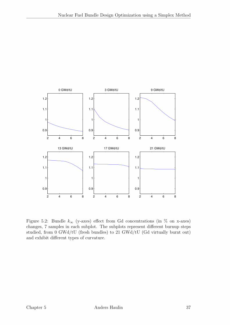
Nuclear Fuel Bundle Design Optimization using a Simplex Method
2 4 6 8
0.9
1
1.1
1.2
0 GWd/tU
2 4 6 8
0.9
1
1.1
1.2
3 GWd/tU
2 4 6 8
0.9
1
1.1
1.2
9 GWd/tU
2 4 6 8
0.9
1
1.1
1.2
13 GWd/tU
2 4 6 8
0.9
1
1.1
1.2
17 GWd/tU
2 4 6 8
0.9
1
1.1
1.2
21 GWd/tU
Figure 5.2: Bundle k∞ (y-axes) effect from Gd concentrations (in % on x-axes)changes, 7 samples in each subplot. The subplots represent different burnup stepsstudied, from 0 GWd/tU (fresh bundles) to 21 GWd/tU (Gd virtually burnt out)and exhibit different types of curvature.
Chapter 5 Anders Haulin 37
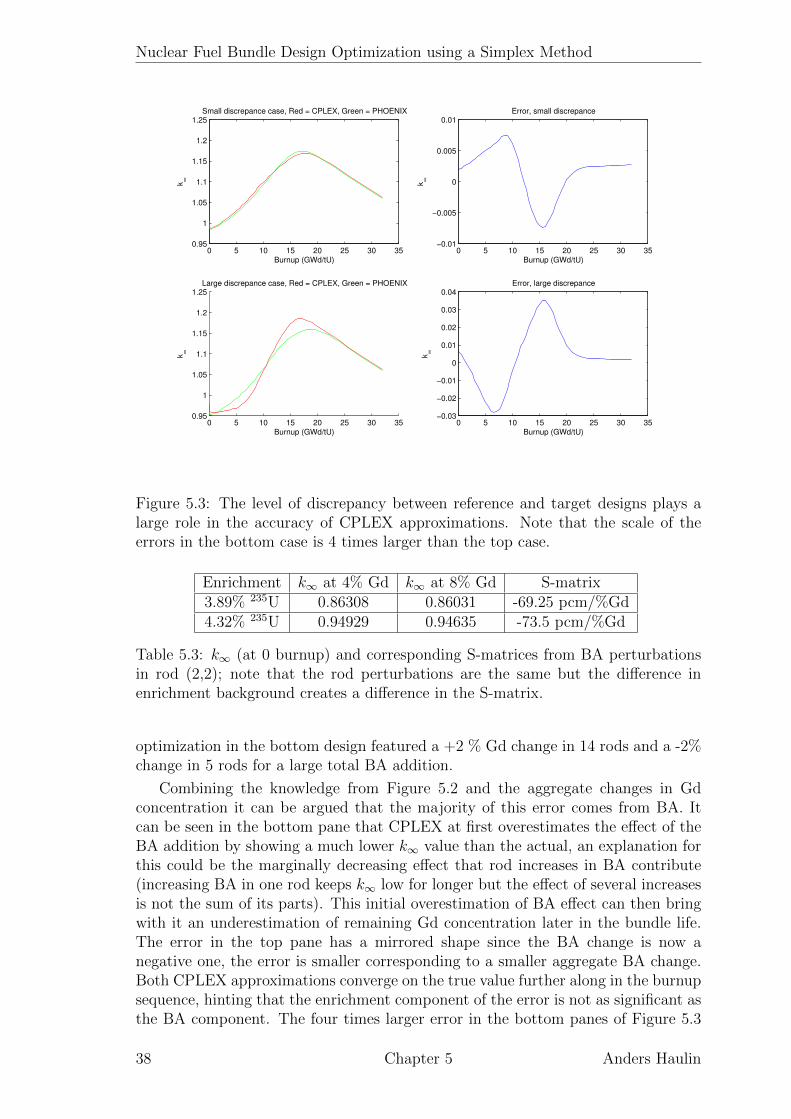
Nuclear Fuel Bundle Design Optimization using a Simplex Method
0 5 10 15 20 25 30 350.95
1
1.05
1.1
1.15
1.2
1.25
Burnup (GWd/tU)
Small discrepance case, Red = CPLEX, Green = PHOENIX
k∞
0 5 10 15 20 25 30 35−0.01
−0.005
0
0.005
0.01
Burnup (GWd/tU)
k∞
Error, small discrepance
0 5 10 15 20 25 30 350.95
1
1.05
1.1
1.15
1.2
1.25
Burnup (GWd/tU)
k∞
Large discrepance case, Red = CPLEX, Green = PHOENIX
0 5 10 15 20 25 30 35−0.03
−0.02
−0.01
0
0.01
0.02
0.03
0.04
Burnup (GWd/tU)
Error, large discrepance
k∞
Figure 5.3: The level of discrepancy between reference and target designs plays alarge role in the accuracy of CPLEX approximations. Note that the scale of theerrors in the bottom case is 4 times larger than the top case.
Enrichment k∞ at 4% Gd k∞ at 8% Gd S-matrix3.89% 235U 0.86308 0.86031 -69.25 pcm/%Gd4.32% 235U 0.94929 0.94635 -73.5 pcm/%Gd
Table 5.3: k∞ (at 0 burnup) and corresponding S-matrices from BA perturbationsin rod (2,2); note that the rod perturbations are the same but the difference inenrichment background creates a difference in the S-matrix.
optimization in the bottom design featured a +2 % Gd change in 14 rods and a -2%change in 5 rods for a large total BA addition.
Combining the knowledge from Figure 5.2 and the aggregate changes in Gdconcentration it can be argued that the majority of this error comes from BA. Itcan be seen in the bottom pane that CPLEX at first overestimates the effect of theBA addition by showing a much lower k∞ value than the actual, an explanation forthis could be the marginally decreasing effect that rod increases in BA contribute(increasing BA in one rod keeps k∞ low for longer but the effect of several increasesis not the sum of its parts). This initial overestimation of BA effect can then bringwith it an underestimation of remaining Gd concentration later in the bundle life.The error in the top pane has a mirrored shape since the BA change is now anegative one, the error is smaller corresponding to a smaller aggregate BA change.Both CPLEX approximations converge on the true value further along in the burnupsequence, hinting that the enrichment component of the error is not as significant asthe BA component. The four times larger error in the bottom panes of Figure 5.3
38 Chapter 5 Anders Haulin

Nuclear Fuel Bundle Design Optimization using a Simplex Method
can, however, be abated by better choosing a reference enrichment to avoid largeenrichment changes and their associated changes in BA concentration. A betterfitting reference design means that the optimization generates smaller changes insecond step and smaller errors in characteristic parameters.
Piecewise linear approximations
Modern simplex optimizers such as CPLEX or Gurobi allow the use of piecewiselinear constraints. In the eyes of the optimizer the calculations representing k∞and other bundle characteristic parameters are merely constraints tying togetherdecision variables (enrichments and BA concentrations) to other decision variables(k∞, Fint and R). Therefore a piecewise calculation could be used to represent anybundle physics; of particular interest for this project was the effect on k∞ from BAchanges in step 25.
2 3 4 5 6 7 80.85
0.9
0.95
1
1.05
1.1
1.15
1.2
1.25
Real k∞
(green), piecewise linear (blue) and linear (red)
Gd concentration (%)
k∞
Figure 5.4: k∞ values from 7 PHOENIX samples (green), linear interpolation be-tween extreme points around the reference (red) and piecewise on each side of thereference (blue).
The appeal of piecewise linear approximations is displayed in Figure 5.4 whereit can be seen that the error arising from linearizing typical BA behavior can besignificantly decreased by using a piecewise approximation. This implementationbetter utilizes the available data, note that no new PHOENIX calculations are nec-essary6 since the perturbation scheme calculates the two extreme points for everyfuel rod position, along with a reference case used as a midpoint7. This gain does,
5k∞-errors can disqualify an optimization and BA changes are their most likely culprit.6Additional intermediary calculations in the S-matrix machinery are however necessary, but
none involving the 2D lattice code.7If the curve is to be divided by a piecewise linear function of more segments than two, new
PHOENIX calculations would be required.
Chapter 5 Anders Haulin 39

Nuclear Fuel Bundle Design Optimization using a Simplex Method
however, come at the cost of approximating every decision variable under piecewiselinear constraints as two separate variables8: in our case one positive and one nega-tive. This increase in variables could prove to be a problem for CPLEX and in thisimplementation it does turn out to be so: calculation time increased 3-fold whilereaching a tolerance 3 times greater than using linear assumptions.
Shadow factors for aggregate BA concentration
Another approach taken to account for non-linear effects of changes in BA concen-tration was to introduce a shadow factor counting the aggregate Gd amount in abundle. Such a factor would then multiply the perturbation element from BA anddecrease or increase its effect. This method was used in the first optimization stepto account for cluster effects of the total amount of BA rods. There the correc-tion for total number of BA rods was added to the BA effect of every rod; sincedecision variables cannot be multiplied with each other (a non-linearity) the binarydecision variable for Gd instead had an extra dimension, so that it was true onlyfor a combination of rod position, Gd concentration and total number of Gd rods9.This would be possible to implement in step 2 as well but the decision variable forGd changes would need a new dimension with one row for every distinction level intotal BA amount. This situation is similar to that of piecewise linear constraints butharder to implement which meant that after the piecewise implementation showedunacceptable increases in computation time it was abandoned.
5.2.2 Power distribution
The power distribution calculations showed some behavior similar to k∞ with burn-able absorber positions being most susceptible to errors. Figure 5.5 shows how theintroduction of BA into 10 positions affect the accuracy of S-matrix calculationcompared to 2D lattice code output.
Figure 5.6 shows the same differences as Figure 5.5 but later in the burnup rangewhere k∞ peaks, it is evident (and not very surprising) that the large approximationerrors in pin powers for a fresh bundle decline greatly as the total effect of BA on thebundle fades. This time in the cycle is the time where approximation error are mostimportant since it is the time at which total power output in the bundle will peak.The errors in pin power estimation will be of great importance to the alternativeR-factor optimizations discussed in Section 5.2.3.
Step 2 optimizations exhibit smaller errors since the Gd rod positions are fixedand thus avoiding strong coupling interaction non-linearities. In an initial statesuch as Figure 5.7 the largest errors arise in the corner rods where also the power isinitially the highest (due to the greater thermal neutron flux).
Indeed, adjusting the errors in Figure 5.7 for the local power in every rod bydividing the error with the rod’s power shows that the relative errors are all below2 %, this can be seen in Figure A.3. The maximum absolute errors in the middleslice without rods in the corners are smaller, as are the errors later in the bundlelife at high burnup, see Figure A.4.
8Or rather as one variable with an extra 0, 1, ... , npieces dimension added representing whichpiece the change in question is along.
9Additional logical constraints then had to link the total number of Gd rods to individualtrue/false values.
40 Chapter 5 Anders Haulin

Nuclear Fuel Bundle Design Optimization using a Simplex Method
Bottom Slice, 0 GWd/tU
-0.008 -0.004 -0.005 -0.007 -0.011 -0.012 -0.006 -0.002 -0.006 -0.011
-0.004 0.092 0.009 -0.008 -0.007 -0.007 0.039 0.007 0.05 -0.008
-0.005 0.009 0.03 -0.004 -0.013 -0.01 0.001 0.005 0.007 -0.005
-0.007 -0.008 -0.004 -0.009 -0.012 -0.009 -0.011 -0.003 0.037 -0.01
-0.011 -0.007 -0.013 -0.012 0 0 -0.013 -0.01 -0.009 -0.009
-0.012 -0.007 -0.01 -0.009 0 0 -0.015 -0.008 -0.008 -0.01
-0.006 0.039 0.001 -0.011 -0.013 -0.015 -0.009 -0.006 -0.003 -0.011
-0.002 0.007 0.005 -0.003 -0.01 -0.008 -0.006 0.029 0.009 -0.005
-0.006 0.05 0.007 0.037 -0.009 -0.008 -0.003 0.009 0.092 -0.005
-0.011 -0.008 -0.005 -0.01 -0.009 -0.01 -0.011 -0.005 -0.005 -0.007
Figure 5.5: Pin power errors at 0 burnup, CPLEX-value minus true PHOENIX valueafter a step-1 optimization. The 10 BA positions coincide with the green areas oflarge positive errors.
Bottom Slice, 7.5 GWd/tU
0.001 0.003 -0.002 0.003 -0.001 -0.001 0.001 0.001 0.004 -0.001
0.003 -0.004 0.001 -0.003 -0.002 -0.003 -0.006 0.002 0.001 0.003
-0.002 0.001 -0.006 0.002 0 0 -0.001 0 -0.005 0.002
0.003 -0.003 0.002 0.004 0 -0.003 0.001 0.001 -0.005 -0.002
-0.001 -0.002 0 0 0 0 0.004 0.001 0 0.003
-0.001 -0.003 0 -0.003 0 0 0.002 0.001 0 0.002
0.001 -0.006 -0.001 0.001 0.004 0.002 0.003 -0.002 0.002 0.004
0.001 0.002 0 0.001 0.001 0.001 -0.002 -0.006 -0.004 0.002
0.004 0.001 -0.005 -0.005 0 0 0.002 -0.004 -0.003 0
-0.001 0.003 0.002 -0.002 0.003 0.002 0.004 0.002 0 0
Figure 5.6: Pin power errors at 7.5 GWd/tU burnup, CPLEX-value minus truePHOENIX value at the burnup point where maximum k∞ appears. The errors fromBA introduction have this late in the bundle life declined considerably (comparedto Figure 5.5, note that the color scales in the figures are not the same and thatabsolute error magnitudes have decreased).
The overall behavior of pin power approximations is acceptable and the strategyof summing contributions from every rod upon every rod is working, albeit requiringa lot of memory for perturbation matrices.
5.2.3 R-factor
The R-factor calculations proved to be the hardest part of the project to evaluate,errors proliferated in the codes and many weighting factors interplayed to obscurethe source of every error. It was time-consuming work to obtain a licensed software,DOFACT, of the right version that could calculate the R-factor. A MATLAB scriptwas also written to do these calculations and extend the cases for which R-factorscould be estimated to those with relative power distributions from other sources thanthe 2D lattice code. Comparisons between R-factor values from simplex approxima-tions, DOFACT and MATLAB were done to gauge the accuracy of optimization.
Chapter 5 Anders Haulin 41

Nuclear Fuel Bundle Design Optimization using a Simplex Method
Bottom Slice, 0 GWd/tU
-0.022 0.003 0.008 0.001 0.001 0.002 0.001 0.008 0.003 -0.022
0.003 -0.001 0.000 -0.001 0.003 0.003 -0.001 0.000 0.000 0.004
0.008 0.000 0.002 0.002 0.000 0.000 0.003 0.001 0.001 0.009
0.000 -0.001 0.002 0.000 -0.003 -0.004 -0.001 0.003 0.000 0.001
0.001 0.003 -0.001 -0.003 0.000 0.000 0.000 0.000 0.004 0.002
0.001 0.002 0.000 -0.004 0.000 0.000 0.001 0.000 0.003 0.002
0.000 -0.001 0.002 -0.001 0.000 0.001 -0.002 0.002 0.000 0.000
0.007 0.000 0.000 0.003 0.000 0.000 0.002 -0.001 0.001 0.007
0.002 -0.001 0.000 -0.001 0.003 0.003 -0.001 0.000 -0.001 0.002
-0.023 0.003 0.008 0.000 0.000 0.001 0.000 0.007 0.002 -0.023
Middle Slice, 0 GWd/tU
0 -0.002 0.004 -0.001 0.000 0.001 0.000 0.006 0.001 0
-0.002 0.000 -0.002 0.001 0.002 0.002 0.003 -0.001 0.002 0
0.004 -0.002 0.000 0.002 0.001 0.000 0.001 0.002 -0.001 0.004
-0.002 0.001 0.002 0.000 -0.004 -0.004 0.000 0.001 0.000 -0.001
0.000 0.002 0.001 -0.004 0 0 -0.001 0.000 0.002 0.001
0.000 0.002 -0.001 -0.004 0 0 -0.001 -0.001 0.002 0.001
-0.001 0.002 0.000 0.000 -0.001 -0.001 0.000 0.001 -0.001 -0.002
0.005 -0.002 0.002 0.001 -0.001 -0.001 0.001 0.002 -0.001 0.004
0.000 0.001 -0.001 0.000 0.001 0.002 -0.001 -0.001 -0.001 0.000
0.000 -0.002 0.003 -0.002 0.000 0.000 -0.002 0.003 0.000 0
Bottom Slice, 18 GWd/tU
0.000 0.001 0.000 0.000 0.000 0.000 0.000 0.001 -0.001 0.001
0.001 -0.002 0.000 -0.001 0.000 0.001 0.003 0.000 -0.001 -0.001
0.000 0.000 0.001 -0.001 -0.002 0.000 0.001 -0.002 0.000 0.000
0.000 -0.001 -0.001 -0.001 -0.001 -0.001 0.000 0.001 -0.001 -0.001
0.000 0.000 -0.002 -0.001 0.000 0.000 0.000 0.000 0.000 0.000
0.000 0.001 0.000 -0.001 0.000 0.000 0.000 -0.001 0.001 0.000
0.000 0.003 0.001 0.000 0.000 0.000 0.000 0.002 -0.001 -0.001
0.001 0.000 -0.002 0.000 0.000 -0.001 0.002 0.009 0.002 0.001
-0.001 -0.001 0.000 -0.001 0.000 0.001 -0.001 0.002 -0.001 0.001
0.001 -0.001 0.000 -0.001 -0.001 0.000 -0.001 0.001 0.001 -0.001
Figure 5.7: Pin power errors at 0 GWd/tU, CPLEX-value minus true PHOENIXvalue after a step-2 optimization. This second optimization step exhibits smallererrors than the first step seen in Figure 5.5, notable however are the corner rodswhere the approximation yields comparatively large errors.
The result of an optimization on the R-factor can be seen in Figure 5.8.
The four cases in Figure 5.8 are R-factor from DOFACT (green), R-factor fromCPLEX approximation (red), R-factor from MATLAB script using 2D lattice codepin powers (blue) and R-factor from MATLAB script using linearized pin powers(black).
The inclusion of the MATLAB values is a form of sanity check: to assure thatthe right version of the DOFACT program was used corresponding to the correla-tion equations provided for simplex approximations. By comparing the values fromCPLEX and MATLAB using pin-powers linearized in CPLEX one can see if poten-tial errors arise all across in the linearization scheme or only in the specific R-factorcalculations. In Figure 5.8 the four curves follow each other nicely and the error inthe CPLEX R-factor is on average smaller than the R-factor analytically calculatedfrom the linearized pin power approximated by CPLEX, this could be due to largerlinearization errors in P than R.
An optimization with a slightly different objective run on the same perturbationmatrices from the same reactor did, however, show a different behavior. Figure5.9 demonstrates how the R-factor approximated by CPLEX differs significantlyfrom the true DOFACT value. By looking closely at which rods exhibited themaximum values in these two curves it was found that the limiting rod in CPLEX’simplementation was not the same as the one in DOFACT and that the limiting rodin CPLEX was one that had a higher additive constant than its neighbors but lowerpin power.
Minimum-value simplification
The linearization scheme for the bundle R-factor was thus found to be faulty in anon-trivial manner. The equations for the R-factor, 1.4 to 1.7, were expressed inthe introduction and of special importance is the neighbor weighting functions like
42 Chapter 5 Anders Haulin
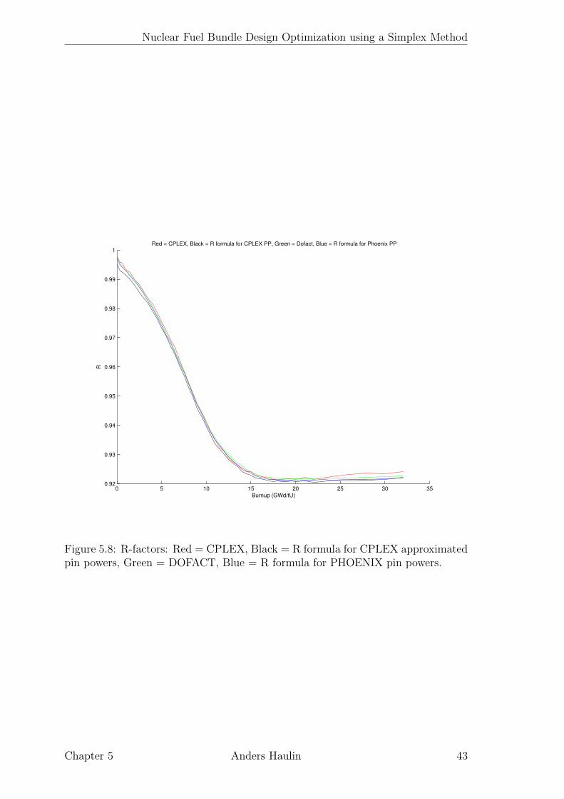
Nuclear Fuel Bundle Design Optimization using a Simplex Method
0 5 10 15 20 25 30 350.92
0.93
0.94
0.95
0.96
0.97
0.98
0.99
1Red = CPLEX, Black = R formula for CPLEX PP, Green = Dofact, Blue = R formula for Phoenix PP
Burnup (GWd/tU)
R
Figure 5.8: R-factors: Red = CPLEX, Black = R formula for CPLEX approximatedpin powers, Green = DOFACT, Blue = R formula for PHOENIX pin powers.
Chapter 5 Anders Haulin 43

Nuclear Fuel Bundle Design Optimization using a Simplex Method
0 5 10 15 20 25 30 350.9
0.91
0.92
0.93
0.94
0.95
0.96Step 1 R−factor, Red = CPLEX, Green = DOFACT
Burnup (GWd/tU)
R
Figure 5.9: R-factors: Red = CPLEX, Green = DOFACT.
44 Chapter 5 Anders Haulin
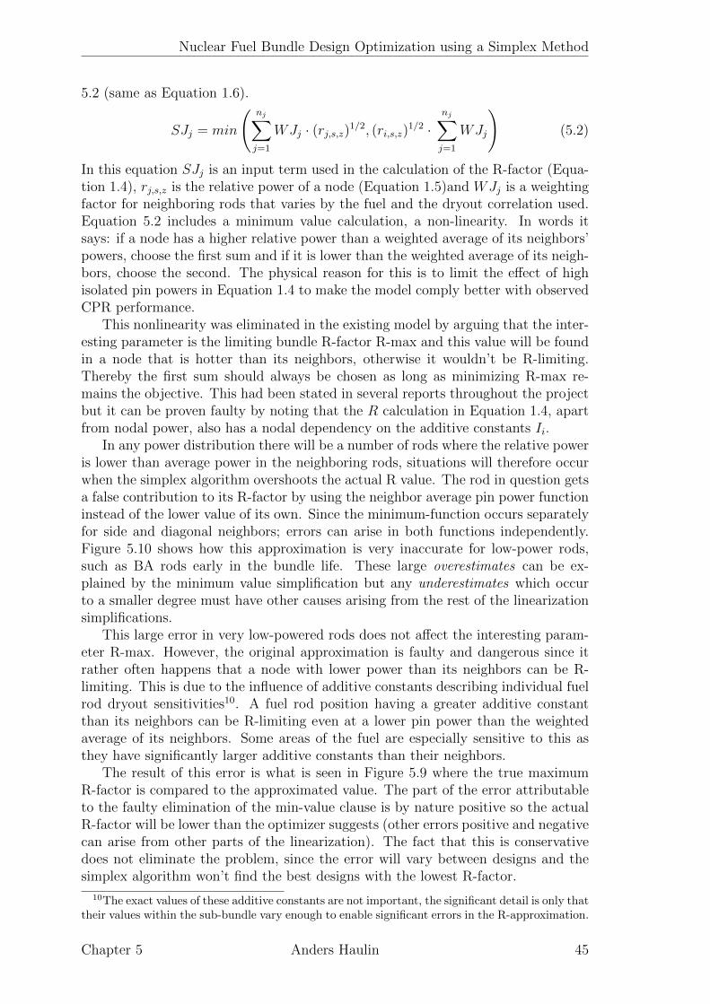
Nuclear Fuel Bundle Design Optimization using a Simplex Method
5.2 (same as Equation 1.6).
SJj = min
(nj∑j=1
WJj · (rj,s,z)1/2, (ri,s,z)1/2 ·
nj∑j=1
WJj
)(5.2)
In this equation SJj is an input term used in the calculation of the R-factor (Equa-tion 1.4), rj,s,z is the relative power of a node (Equation 1.5)and WJj is a weightingfactor for neighboring rods that varies by the fuel and the dryout correlation used.Equation 5.2 includes a minimum value calculation, a non-linearity. In words itsays: if a node has a higher relative power than a weighted average of its neighbors’powers, choose the first sum and if it is lower than the weighted average of its neigh-bors, choose the second. The physical reason for this is to limit the effect of highisolated pin powers in Equation 1.4 to make the model comply better with observedCPR performance.
This nonlinearity was eliminated in the existing model by arguing that the inter-esting parameter is the limiting bundle R-factor R-max and this value will be foundin a node that is hotter than its neighbors, otherwise it wouldn’t be R-limiting.Thereby the first sum should always be chosen as long as minimizing R-max re-mains the objective. This had been stated in several reports throughout the projectbut it can be proven faulty by noting that the R calculation in Equation 1.4, apartfrom nodal power, also has a nodal dependency on the additive constants Ii.
In any power distribution there will be a number of rods where the relative poweris lower than average power in the neighboring rods, situations will therefore occurwhen the simplex algorithm overshoots the actual R value. The rod in question getsa false contribution to its R-factor by using the neighbor average pin power functioninstead of the lower value of its own. Since the minimum-function occurs separatelyfor side and diagonal neighbors; errors can arise in both functions independently.Figure 5.10 shows how this approximation is very inaccurate for low-power rods,such as BA rods early in the bundle life. These large overestimates can be ex-plained by the minimum value simplification but any underestimates which occurto a smaller degree must have other causes arising from the rest of the linearizationsimplifications.
This large error in very low-powered rods does not affect the interesting param-eter R-max. However, the original approximation is faulty and dangerous since itrather often happens that a node with lower power than its neighbors can be R-limiting. This is due to the influence of additive constants describing individual fuelrod dryout sensitivities10. A fuel rod position having a greater additive constantthan its neighbors can be R-limiting even at a lower pin power than the weightedaverage of its neighbors. Some areas of the fuel are especially sensitive to this asthey have significantly larger additive constants than their neighbors.
The result of this error is what is seen in Figure 5.9 where the true maximumR-factor is compared to the approximated value. The part of the error attributableto the faulty elimination of the min-value clause is by nature positive so the actualR-factor will be lower than the optimizer suggests (other errors positive and negativecan arise from other parts of the linearization). The fact that this is conservativedoes not eliminate the problem, since the error will vary between designs and thesimplex algorithm won’t find the best designs with the lowest R-factor.
10The exact values of these additive constants are not important, the significant detail is only thattheir values within the sub-bundle vary enough to enable significant errors in the R-approximation.
Chapter 5 Anders Haulin 45
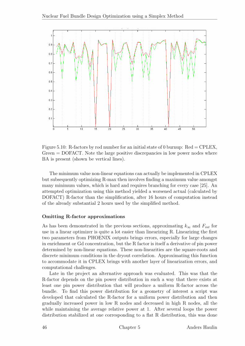
Nuclear Fuel Bundle Design Optimization using a Simplex Method
Figure 5.10: R-factors by rod number for an initial state of 0 burnup: Red = CPLEX,Green = DOFACT. Note the large positive discrepancies in low power nodes whereBA is present (shown be vertical lines).
The minimum value non-linear equations can actually be implemented in CPLEXbut subsequently optimizing R-max then involves finding a maximum value amongstmany minimum values, which is hard and requires branching for every case [25]. Anattempted optimization using this method yielded a worsened actual (calculated byDOFACT) R-factor than the simplification, after 16 hours of computation insteadof the already substantial 2 hours used by the simplified method.
Omitting R-factor approximations
As has been demonstrated in the previous sections, approximating k∞ and Fint foruse in a linear optimizer is quite a lot easier than linearizing R. Linearizing the firsttwo parameters from PHOENIX outputs brings errors, especially for large changesin enrichment or Gd concentration, but the R factor is itself a derivative of pin powerdetermined by non-linear equations. These non-linearities are the square-roots anddiscrete minimum conditions in the dryout correlation. Approximating this functionto accommodate it in CPLEX brings with another layer of linearization errors, andcomputational challenges.
Late in the project an alternative approach was evaluated. This was that theR-factor depends on the pin power distribution in such a way that there exists atleast one pin power distribution that will produce a uniform R-factor across thebundle. To find this power distribution for a geometry of interest a script wasdeveloped that calculated the R-factor for a uniform power distribution and thengradually increased power in low R nodes and decreased in high R nodes, all thewhile maintaining the average relative power at 1. After several loops the powerdistribution stabilized at one corresponding to a flat R distribution, this was done
46 Chapter 5 Anders Haulin
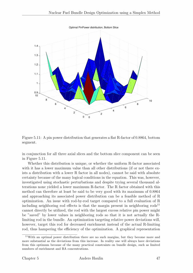
Nuclear Fuel Bundle Design Optimization using a Simplex Method
0
2
4
6
8
10
0
2
4
6
8
100.9
1
1.1
1.2
1.3
1.4
Optimal PinPower distribution, Bottom Slice
Figure 5.11: A pin power distribution that generates a flat R-factor of 0.8864, bottomsegment.
in conjunction for all three axial slices and the bottom slice component can be seenin Figure 5.11.
Whether this distribution is unique, or whether the uniform R-factor associatedwith it has a lower maximum value than all other distributions (if or not there ex-ists a distribution with a lower R factor in all nodes), cannot be said with absolutecertainty because of the many logical conditions in the equation. This was, however,investigated using stochastic perturbations and despite trying several thousand al-terations none yielded a lower maximum R-factor. The R factor obtained with thismethod can therefore at least be said to be very good with its maximum of 0.8864and approaching its associated power distribution can be a feasible method of Roptimization. An issue with rod-by-rod target compared to a full evaluation of Rincluding neighboring rod effects is that the margin present in neighboring rods11
cannot directly be utilized, the rod with the largest excess relative pin power mightbe ”saved” by lower values in neighboring rods so that it is not actually the R-limiting rod in the bundle. An optimization targeting relative power deviations will,however, target this rod for decreased enrichment instead of the actual R-limitingrod, thus hampering the efficiency of the optimization. A graphical representation
11With an optimal power distribution there are no such margins, but they become more andmore substantial as the deviations from this increase. In reality one will always have deviationsfrom this optimum because of the many practical constraints on bundle design, such as limitednumbers of enrichment and BA concentrations.
Chapter 5 Anders Haulin 47
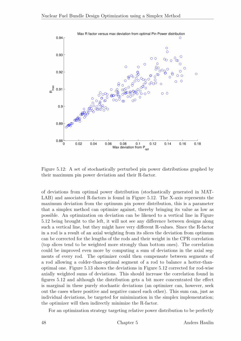
Nuclear Fuel Bundle Design Optimization using a Simplex Method
0 0.02 0.04 0.06 0.08 0.1 0.12 0.14 0.16 0.180.88
0.89
0.9
0.91
0.92
0.93
0.94Max R factor versus max deviation from optimal Pin Power distribution
Rm
ax
Max deviation from Popt
Figure 5.12: A set of stochastically perturbed pin power distributions graphed bytheir maximum pin power deviation and their R-factor.
of deviations from optimal power distribution (stochastically generated in MAT-LAB) and associated R-factors is found in Figure 5.12. The X-axis represents themaximum deviation from the optimum pin power distribution, this is a parameterthat a simplex method can optimize against, thereby bringing its value as low aspossible. An optimization on deviation can be likened to a vertical line in Figure5.12 being brought to the left, it will not see any difference between designs alongsuch a vertical line, but they might have very different R-values. Since the R-factorin a rod is a result of an axial weighting from its slices the deviation from optimumcan be corrected for the lengths of the rods and their weight in the CPR correlation(top slices tend to be weighted more strongly than bottom ones). The correlationcould be improved even more by computing a sum of deviations in the axial seg-ments of every rod. The optimizer could then compensate between segments ofa rod allowing a colder-than-optimal segment of a rod to balance a hotter-than-optimal one. Figure 5.13 shows the deviations in Figure 5.12 corrected for rod-wiseaxially weighted sums of deviations. This should increase the correlation found infigures 5.12 and although the distribution gets a bit more concentrated the effectis marginal in these purely stochastic deviations (an optimizer can, however, seekout the cases where positive and negative cancel each other). This sum can, just asindividual deviations, be targeted for minimization in the simplex implementation;the optimizer will then indirectly minimize the R-factor.
For an optimization strategy targeting relative power distribution to be perfectly
48 Chapter 5 Anders Haulin
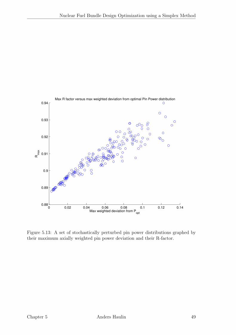
Nuclear Fuel Bundle Design Optimization using a Simplex Method
0 0.02 0.04 0.06 0.08 0.1 0.12 0.140.88
0.89
0.9
0.91
0.92
0.93
0.94Max R factor versus max weighted deviation from optimal Pin Power distribution
Rm
ax
Max weighted deviation from Popt
Figure 5.13: A set of stochastically perturbed pin power distributions graphed bytheir maximum axially weighted pin power deviation and their R-factor.
Chapter 5 Anders Haulin 49
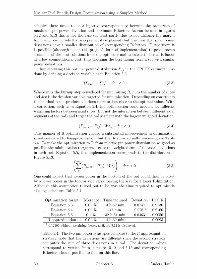
Nuclear Fuel Bundle Design Optimization using a Simplex Method
effective there needs to be a bijective correspondence between the properties ofmaximum pin power deviation and maximum R-factor. As can be seen in figures5.12 and 5.13 this is not the case (at least partly due to not utilizing the marginfrom neighboring rods that was previously explained) but it is clear that small powerdeviations have a smaller distribution of corresponding R-factors. Furthermore itis possible (although not in this project’s form of implementation) to post-processa number of the best solutions from the optimizer and calculate their real R-factorat a low computational cost, thus choosing the best design from a set with similarpower deviations.
Implementing this optimal power distribution P ?z,i in the CPLEX optimizer was
done by defining a decision variable as in Equation 5.3.
(Pz,i,m − P ?z,i)− dev < 0 (5.3)
Where m is the burnup step considered for minimizing R, nz is the number of slicesand dev is the decision variable targeted for minimization. Depending on constraintsthis method could produce solutions more or less close to the optimal value. Witha correction, such as in Equation 5.4, the optimization could account for differentweighting factors between axial slices (but not the interaction between different axialsegments of the rod) and target the rod segment with the largest weighted deviation.
(Pz,i,m − P ?z,i) ·Wzz − dev < 0 (5.4)
This manner of R-optimization yielded a substantial improvement in optimizationspeed compared to R-approximation, but the R-factor actually worsened, see Table5.4. To make the optimization to R from relative pin power distribution as good aspossible the minimization target was set as the weighted sum of the axial deviationsin each rod, Equation 5.5, this implementation corresponds to the distribution inFigure 5.13. (
nz∑z
(Pz,i,m − P ?z,i) ·Wzz
)− dev < 0 (5.5)
One could expect that excess power in the bottom of the rod could then be offsetby a lower power in the top, or vice versa, paving the way for a lower R-limitation.Although this assumption turned out to be true the time required to optimize italso exploded: see Table 5.4.
Optimization target Tolerance Time required Deviation Real REquation 5.3 0.01 % 3 h 59 min 0.0747 0.9130Equation 5.4 0.01 % 47 min 0.026 1 0.9166Equation 5.5 0.1 % 32 h 51 min 0.0463 0.9056
R approximation 0.01 % 4 h 30 min - 0.90931 0.12406 without weighting factor, as figure 5.12 is displayed.
Table 5.4: The two pin power strategies compare to the R approximationstrategy, note that the deviations are different since the second strategycomputes the sum of three deviations in a rod. The deviation valuescorrespond to vertical lines in figures 5.12 and 5.13 and correspondingR-factors should possible to find on this line.
50 Chapter 5 Anders Haulin

Nuclear Fuel Bundle Design Optimization using a Simplex Method
The comparison in Table 5.4 to the design obtained by R approximation showsthat the pin power deviation minimization can indeed generate a superior designbut at a high cost in calculation time. The reasons for this have not been firmlyestablished but it could be due to the greater number of variables considered in theoptimization.
In the calculations of Table 5.4 several constraints applied to the optimizationbesides the optimization target function; one of these was a constraint on LHGR (seeSection 1.2.3): effectively one on Fint on the bundle level. This constraint dependedon burnup and in the optimization interval it was as low as 1.19 while the optimumcorner rod power was 1.3276. This constraint inhibits the optimization and makesit harder to reach optimal power profile in Figure 5.11. By forcing rods to remaincolder than their optimum it is possible that the coupling between optimizing powerprofile and optimizing R-factor weakens. A possible way of improving this is toincorporate the limitation on LHGR in the generation of an optimal power profile,thus this profile will depend on the constraints and needs to be re-generated if theconstraint or targeted burnup interval changes. This condition did not, however,change the optimum power profile much outside the corner rods, and the ”penalty”to the R-factor was small as it rose from 0.8864 to 0.8870. It became clear thatincluding the constraint did not, however, improve the optimization, the optimizerreached R = 0.9058, or just above the previous best value, but CPLEX was noteven approaching termination after 48 hours and 7583022 iterations so the idea wasdiscarded.
5.3 Optimized layout results
The previous sections concerned the methods used in optimization and the improve-ments that could be done to these. The questions of errors prevalent in the CPLEXoptimization are important but the main objective or the optimization framework isto speed up the fuel design process and therefore a study comparing automaticallyoptimized designs to those made by nuclear engineers using experience, trial anderror was conducted. The method and the cases for this study were described inSection 3.3. The alternative methods for calculating the R-factor discussed in Sec-tion 5.2.3 were not implemented in these optimizations as a time-efficient methodfor this had not been found.
5.3.1 BA rod position optimization
The first step in these optimizations was to generate a reference design to startthe process from. This reference design had previously been one with maximum-enriched in all non-peripheral rods but since it was found that large deviations inenrichment increased the errors of the linearization model the reference was insteadcalculated to be as close as possible to the desired enrichment. For the short-cyclereactor this was done by simply taking the design from the manual design in Figure5.14, replacing its BA rods with pure uranium and adjusting the layout so that allinterior rod positions had the same enrichment and total bundle average enrichmentwas preserved. This design shown in Figure 5.15 was then perturbed with Gd inconcentrations of 2, 3, 4 and 6 % in every permitted position. This amounted to116 designs per bundle segment.
Chapter 5 Anders Haulin 51
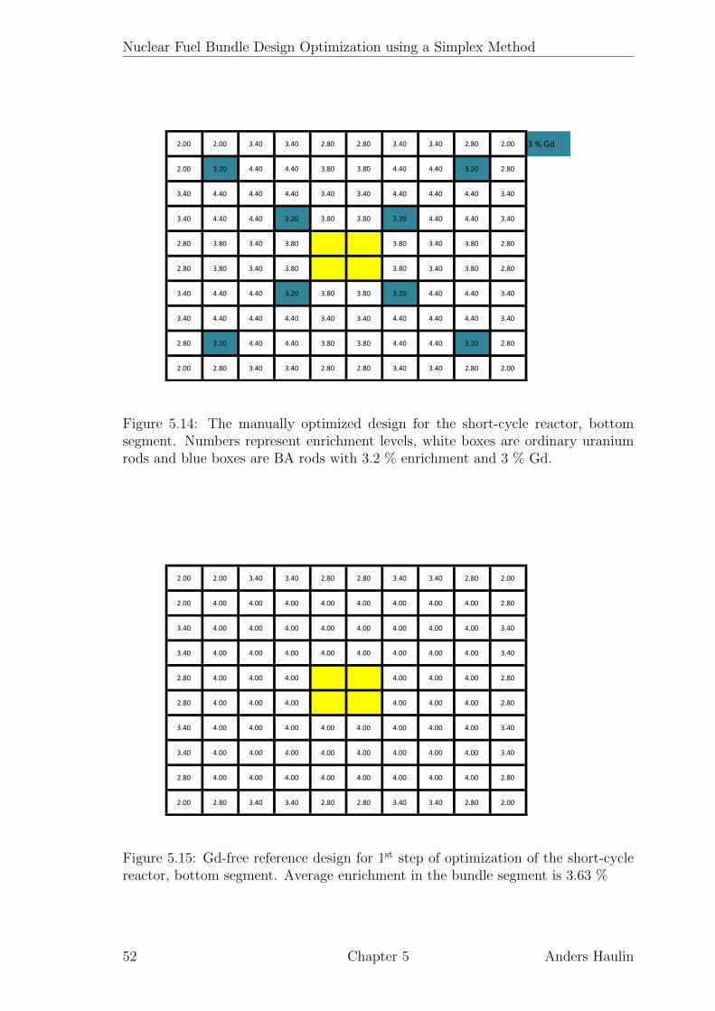
Nuclear Fuel Bundle Design Optimization using a Simplex Method
2.00 2.00 3.40 3.40 2.80 2.80 3.40 3.40 2.80 2.00 3 % Gd
2.00 3.20 4.40 4.40 3.80 3.80 4.40 4.40 3.20 2.80
3.40 4.40 4.40 4.40 3.40 3.40 4.40 4.40 4.40 3.40
3.40 4.40 4.40 3.20 3.80 3.80 3.20 4.40 4.40 3.40
2.80 3.80 3.40 3.80 3.80 3.40 3.80 2.80
2.80 3.80 3.40 3.80 3.80 3.40 3.80 2.80
3.40 4.40 4.40 3.20 3.80 3.80 3.20 4.40 4.40 3.40
3.40 4.40 4.40 4.40 3.40 3.40 4.40 4.40 4.40 3.40
2.80 3.20 4.40 4.40 3.80 3.80 4.40 4.40 3.20 2.80
2.00 2.80 3.40 3.40 2.80 2.80 3.40 3.40 2.80 2.00
2 2 3.4 3.4 2.8 2.8 3.4 3.4 2.8 2
2 3.2 4.4 4.4 3.8 3.8 4.4 4.4 3.2 2.8
3.4 4.4 4.4 4.4 3.4 3.4 4.4 4.4 4.4 3.4
3.4 4.4 4.4 3.2 3.8 3.8 3.2 4.4 4.4 3.4
2.8 3.8 3.4 3.8 3.8 3.4 3.8 2.8
2.8 3.8 3.4 3.8 3.8 3.4 3.8 2.8
3.4 4.4 4.4 3.2 3.8 3.8 3.2 4.4 4.4 3.4
3.4 4.4 4.4 4.4 3.4 3.4 4.4 4.4 4.4 3.4
2.8 3.2 4.4 4.4 3.8 3.8 4.4 4.4 3.2 2.8
2 2.8 3.4 3.4 2.8 2.8 3.4 3.4 2.8 2
Figure 5.14: The manually optimized design for the short-cycle reactor, bottomsegment. Numbers represent enrichment levels, white boxes are ordinary uraniumrods and blue boxes are BA rods with 3.2 % enrichment and 3 % Gd.
2.00 2.00 3.40 3.40 2.80 2.80 3.40 3.40 2.80 2.00
2.00 4.00 4.00 4.00 4.00 4.00 4.00 4.00 4.00 2.80
3.40 4.00 4.00 4.00 4.00 4.00 4.00 4.00 4.00 3.40
3.40 4.00 4.00 4.00 4.00 4.00 4.00 4.00 4.00 3.40
2.80 4.00 4.00 4.00 4.00 4.00 4.00 2.80
2.80 4.00 4.00 4.00 4.00 4.00 4.00 2.80
3.40 4.00 4.00 4.00 4.00 4.00 4.00 4.00 4.00 3.40
3.40 4.00 4.00 4.00 4.00 4.00 4.00 4.00 4.00 3.40
2.80 4.00 4.00 4.00 4.00 4.00 4.00 4.00 4.00 2.80
2.00 2.80 3.40 3.40 2.80 2.80 3.40 3.40 2.80 2.00
Figure 5.15: Gd-free reference design for 1st step of optimization of the short-cyclereactor, bottom segment. Average enrichment in the bundle segment is 3.63 %
52 Chapter 5 Anders Haulin

Nuclear Fuel Bundle Design Optimization using a Simplex Method
2.80 2.80 3.80 3.80 3.80 3.80 3.80 4.60 3.80 2.80
2.80 3.80 4.95 4.2 & 7 % 4.95 4.95 4.95 4.95 4.2 & 5% 3.80
3.80 4.95 4.2 & 7 % 4.95 4.95 4.95 4.2 & 7 % 4.95 4.95 4.60
3.80 4.2 & 7 % 4.95 4.95 4.95 4.95 4.95 4.2 & 7 % 4.95 4.60
3.80 4.95 4.95 4.95 - - 4.95 4.95 4.95 3.80
3.80 4.95 4.95 4.95 - - 4.95 4.95 4.2 & 7 % 3.80
3.80 4.95 4.2 & 7 % 4.95 4.95 4.95 4.95 4.2 & 7 % 4.95 4.60
4.60 4.95 4.95 4.2 & 7 % 4.95 4.95 4.2 & 7 % 4.95 4.2 & 7 % 4.60
3.80 4.2 & 5% 4.95 4.95 4.95 4.2 & 7 % 4.95 4.2 & 7 % 4.20 3.80
2.80 3.80 4.60 4.60 3.80 3.80 4.60 4.60 3.80 2.80
Figure 5.16: The manually optimized design for the long-cycle reactor, bottom seg-ment. Numbers without percentages represent enrichments, colored boxes representBA rods with percentages stating Gd concentration.
The procedure was identical for the long-cycle reactor although the referencedesign was instead Figure 5.16 and Gd perturbation concentrations were 4, 6 and 8%.
The perturbations generated a set of step 1 S-matrices which were run in theCPLEX optimization suite. The optimization was subject to numerous constraintsincluding those detailed in Table 3.1 and properties derived from the final designs,namely the peak k∞ burnup, b and the BA effect on initial k∞, a. Table 5.5 showsthe details of the step 1 optimizations. The documentation for manual design ofthe short cycle reactor stated that the design was optimized towards minimizingFint. Such a strategy can be implemented in the simplex optimizer but the resultingdesigns proved very poor with regard to R and it proved more efficient to includeR in the optimization target than trying to constrain it under fixed values, a largeimprovement in R-factor was then obtained from a much smaller sacrifice in Fint.
For the short-cycle reactor a CPLEX approximated R-factor along with its realDOFACT value can be seen in Figure 5.17, the CPLEX approximation shown inred is the curve approximated by CPLEX for its winning design. An evaluation ofthis suggested design shows that its real R-factor is actually lower than the CPLEXapproximation through the majority of the bundle life.
That the CPLEX approximation in Figure 5.17 for R overshoots the real valuecan be explained by the errors observed from the faulty but necessary simplificationof the minimum function SJ and SK in the R approximation.
5.3.2 Uranium enrichment and Gd concentration optimiza-tion
The BA placements from step 1 were taken as references for a step 2 optimizationwhere BA positions were fixed and perturbations ran for every position in the grid.
Chapter 5 Anders Haulin 53
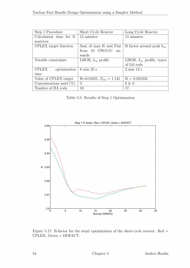
Nuclear Fuel Bundle Design Optimization using a Simplex Method
Step 1 Procedure Short Cycle Reactor Long Cycle ReactorCalculation time for S-matrices
15 minutes 15 minutes
CPLEX target function Sum of max R and Fintfrom 10 GWd/tU on-wards
R factor around peak k∞
Notable constraints LHGR, k∞ profile LHGR, k∞ profile, typesof Gd rods
CPLEX optimizationtime
8 min 25 s 2 min 12 s
Value of CPLEX target R=0.91651, Fint = 1.141 R = 0.921033Concentrations used (%) 3 6 & 8Number of BA rods 10 17
Table 5.5: Results of Step 1 Optimization
0 5 10 15 20 25 30 350.9
0.91
0.92
0.93
0.94
0.95
0.96Step 1 R−factor, Red = CPLEX, Green = DOFACT
Burnup (GWd/tU)
R
Figure 5.17: R-factor for the step1 optimization of the short-cycle reactor. Red =CPLEX, Green = DOFACT.
54 Chapter 5 Anders Haulin
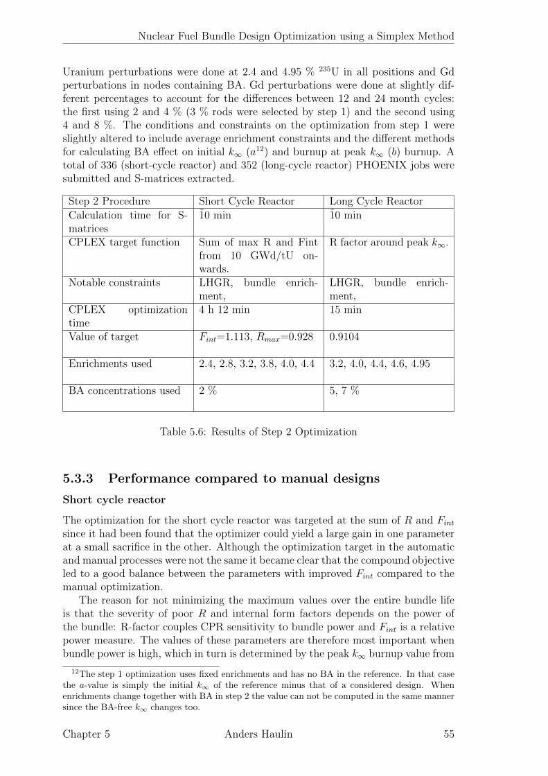
Nuclear Fuel Bundle Design Optimization using a Simplex Method
Uranium perturbations were done at 2.4 and 4.95 % 235U in all positions and Gdperturbations in nodes containing BA. Gd perturbations were done at slightly dif-ferent percentages to account for the differences between 12 and 24 month cycles:the first using 2 and 4 % (3 % rods were selected by step 1) and the second using4 and 8 %. The conditions and constraints on the optimization from step 1 wereslightly altered to include average enrichment constraints and the different methodsfor calculating BA effect on initial k∞ (a12) and burnup at peak k∞ (b) burnup. Atotal of 336 (short-cycle reactor) and 352 (long-cycle reactor) PHOENIX jobs weresubmitted and S-matrices extracted.
Step 2 Procedure Short Cycle Reactor Long Cycle Reactor
Calculation time for S-matrices
10 min 10 min
CPLEX target function Sum of max R and Fintfrom 10 GWd/tU on-wards.
R factor around peak k∞.
Notable constraints LHGR, bundle enrich-ment,
LHGR, bundle enrich-ment,
CPLEX optimizationtime
4 h 12 min 15 min
Value of target Fint=1.113, Rmax=0.928 0.9104
Enrichments used 2.4, 2.8, 3.2, 3.8, 4.0, 4.4 3.2, 4.0, 4.4, 4.6, 4.95
BA concentrations used 2 % 5, 7 %
Table 5.6: Results of Step 2 Optimization
5.3.3 Performance compared to manual designs
Short cycle reactor
The optimization for the short cycle reactor was targeted at the sum of R and Fint
since it had been found that the optimizer could yield a large gain in one parameterat a small sacrifice in the other. Although the optimization target in the automaticand manual processes were not the same it became clear that the compound objectiveled to a good balance between the parameters with improved Fint compared to themanual optimization.
The reason for not minimizing the maximum values over the entire bundle lifeis that the severity of poor R and internal form factors depends on the power ofthe bundle: R-factor couples CPR sensitivity to bundle power and Fint is a relativepower measure. The values of these parameters are therefore most important whenbundle power is high, which in turn is determined by the peak k∞ burnup value from
12The step 1 optimization uses fixed enrichments and has no BA in the reference. In that casethe a-value is simply the initial k∞ of the reference minus that of a considered design. Whenenrichments change together with BA in step 2 the value can not be computed in the same mannersince the BA-free k∞ changes too.
Chapter 5 Anders Haulin 55

Nuclear Fuel Bundle Design Optimization using a Simplex Method
2.40 2.40 3.20 3.20 2.80 2.80 3.20 3.20 2.40 2.40 2 % Gd
2.40 3.20 4.00 4.40 4.40 4.40 4.40 4.00 3.20 2.40
3.20 4.00 3.20 4.40 4.00 4.00 4.40 4.40 4.00 3.20
3.20 4.40 4.40 3.80 4.00 4.00 3.80 4.40 3.80 3.20
2.80 4.40 4.00 4.00 4.00 3.80 4.40 2.80
2.80 4.40 4.00 4.00 4.00 3.80 4.40 2.80
3.20 4.40 4.40 3.80 4.00 4.00 3.80 4.40 4.40 3.20
3.20 4.00 4.40 4.40 3.80 3.80 4.40 3.20 4.00 3.20
2.40 3.20 4.00 3.80 4.40 4.40 4.40 4.00 3.20 2.40
2.40 2.40 3.20 3.20 2.80 2.80 3.20 3.20 2.40 2.40
Figure 5.18: Automatically optimized design for the short-cycle reactor.
k∞ optimization. It is also useful that narrowing the burnup interval over whichoptimization is done decreases the number of points CPLEX needs to evaluate andtherefore the run-time.
The automatic optimization for the short cycle reactor was found to performwell against the manually optimized reference design on several criteria, the internalform factor in Figure 5.20 was kept lower during peak k∞ by sacrificing some initialand final margin. For the bottom slice studied internal form factor at 0 burnupincreased from 1.186 to 1.204, at peak k∞ decreased from 1.11 to 1.079 and at 40GWd/tU it increased from 1.046 to 1.055.
The R-factor was included in the optimization and this made a mark since itmanaged to perform better than the manual design throughout the cycle, see Figure5.21. The k∞ profile was a bit off from the desired peak k∞ burnup as seen inFigure 5.22, this proved to be the result of a combination of lax CPLEX constraintsand linearization inaccuracy. The sought profile of the manual optimization peakedat 7 GWd/tU whereas the simplex approximation was calculated to do so at 6.5GWd/tU13, the real value for this peak however turned out to be 6.0 GWd/tU afterdesign was evaluated in the 2D lattice code.
Long cycle reactor
For the long-cycle reactor the optimizer had a harder task complying with the con-straints. This manual optimization was well-done and small inaccuracies propagatedin the model to impair the results of the automatic optimization. Figure 5.23 showsthat the optimized design ”wins” in the target interval around 20 GWd/tU, wherethe R-factor decreases from 0.922 to 0.912; but performs worse in other parts of thecycle, for instance at 0 burnup where it increases from 1.020 to 1.053.
Figure 5.24 demonstrates clearer how the gain in R-performance has come at alarge sacrifice in pin power distribution, which is much more unequal than in the
13A tolerance of 0.5 GWd/tU above or below the sought value was used, this can be omitted
56 Chapter 5 Anders Haulin

Nuclear Fuel Bundle Design Optimization using a Simplex Method
3.20 3.20 4.60 4.00 3.20 3.20 4.00 4.95 4.60 4.00
3.20 4.6 & 5% 3.20 4.95 4.6 & 5% 4.6 & 7% 4.60 4.6 & 5% 4.00 4.60
4.60 3.20 4.6 & 5% 4.95 4.60 4.60 4.95 4.95 4.4 & 7% 4.95
4.00 4.95 4.95 4.95 4.40 4.95 4.95 4.95 4.60 4.40
3.20 4.6 & 5% 4.60 4.40 - - 4.60 4.95 4.6 & 5% 3.20
3.20 4.6 & 7% 4.60 4.95 - - 4.95 4.95 4.6 & 5% 3.20
4.00 4.60 4.95 4.95 4.60 4.95 4.4 & 7% 4.95 4.95 4.40
4.95 4.6 & 5% 4.95 4.95 4.95 4.95 4.95 4.95 4.6 & 5% 4.95
4.60 4.00 4.4 & 7% 4.60 4.6 & 5% 4.6 & 5% 4.95 4.6 & 5% 4.00 4.60
4.00 4.60 4.95 4.40 3.20 3.20 4.40 4.95 4.60 4.00
Figure 5.19: Automatically optimized design for the long-cycle reactor.
manual case: initial Fint increases from 1.354 to 1.617 and Fint at peak k∞ from1.118 to 1.147.
The result of this optimization showed the importance of balanced constraints, asthe maximum relative pin power in Figure 5.24 is quite unacceptable. Attemptingto correct the pay-off between Fint and R new optimizations were therefore run,targeting the sum of R in the target interval and Fint (just as in the short-cyclereactor optimizations) over a larger burnup interval. Different weight factors forR and Fint were used in defining an optimization variable and the best overallperformance came with the R contribution targeted twice as heavy as Fint part,thus by defining the target variable t as t = Fint
2+R.
The results of this alternative strategy can be seen in figures 5.25 and 5.26. It isclear that no gain in one parameter came without sacrificing the other but it showsto the feasibility of using weighted sums of parameters as optimization targets14.The role and potential benefits of unconventional compound objectives is discussedin Section 6.1.4.
For the long-cycle reactor neither the optimization targeting only R nor the oneusing a compound R and Fint target could generate any overall improvements tothe manual design in the manner that the short cycle reactor optimization could (atleast on a first glance).
Time savings
It should be noted that the manual design in the long-cycle reactor case did indeedrequire significant design time and represents exactly the kind of case an optimiza-tion program is requested for. Actually quantifying the time taken to design a fuelbundle is hard since the process is intertwined with the general core design processbut estimates on tough cases range as high as one engineering-week.
14If there is time; a greater number of parameters evaluated increases the run-time significantly,especially if they have to be evaluated over longer burnup intervals.
Chapter 5 Anders Haulin 57

Nuclear Fuel Bundle Design Optimization using a Simplex Method
0 10 20 30 40 50 601.02
1.04
1.06
1.08
1.1
1.12
1.14
1.16
1.18
1.2
1.22
Burnup (GWd/tU)
Fin
t
Fint
bottom slice, Red = Manual design , Green = Automatic
Figure 5.20: Short-cycle reactor bottom slice maximum relative pin power, red =manual design, green = automatic design.
0 10 20 30 40 50 600.92
0.925
0.93
0.935
0.94
0.945
0.95
0.955
0.96
0.965
Burnup (GWd/tU)
Rm
ax
Rmax
, Red = Manual design , Green = Automatic
Figure 5.21: Short-cycle reactor maximum R-factor, red = manual design, green =automatic design.
58 Chapter 5 Anders Haulin
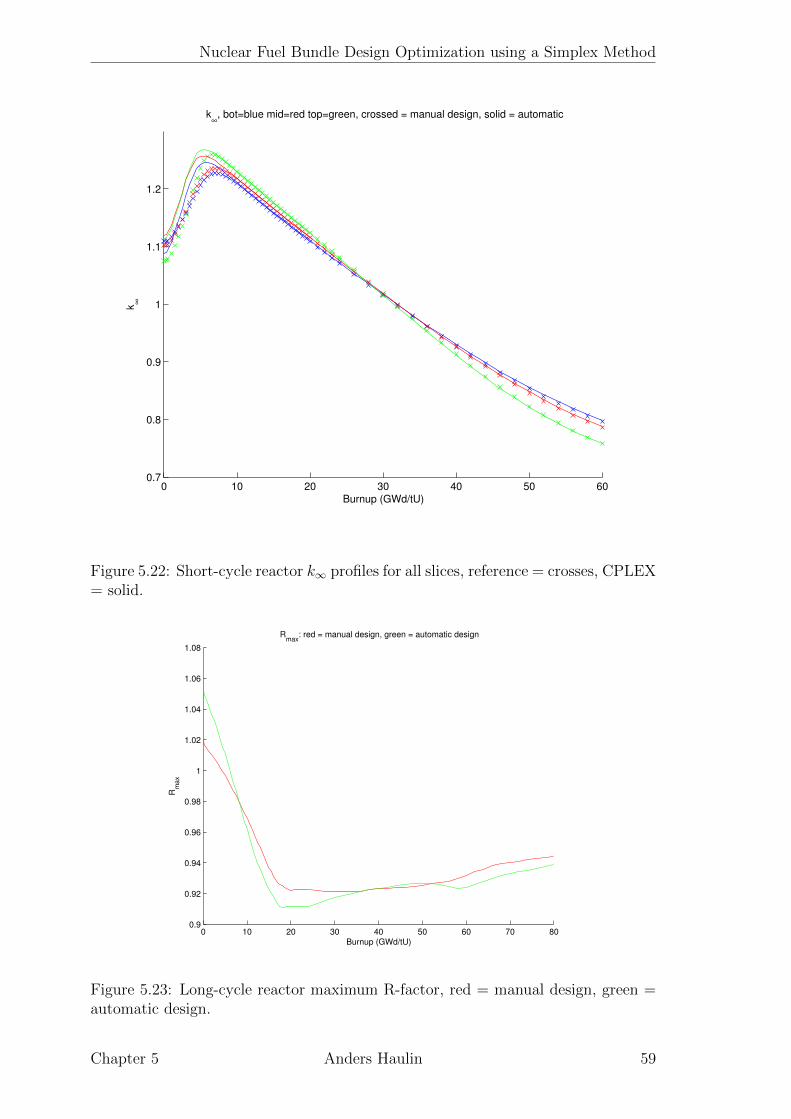
Nuclear Fuel Bundle Design Optimization using a Simplex Method
0 10 20 30 40 50 600.7
0.8
0.9
1
1.1
1.2
Burnup (GWd/tU)
k∞
k∞
, bot=blue mid=red top=green, crossed = manual design, solid = automatic
Figure 5.22: Short-cycle reactor k∞ profiles for all slices, reference = crosses, CPLEX= solid.
0 10 20 30 40 50 60 70 800.9
0.92
0.94
0.96
0.98
1
1.02
1.04
1.06
1.08
Burnup (GWd/tU)
Rm
ax
Rmax
: red = manual design, green = automatic design
Figure 5.23: Long-cycle reactor maximum R-factor, red = manual design, green =automatic design.
Chapter 5 Anders Haulin 59

Nuclear Fuel Bundle Design Optimization using a Simplex Method
0 10 20 30 40 50 60 70 801
1.1
1.2
1.3
1.4
1.5
1.6
1.7
1.8
Burnup (GWd/tU)
Fin
t
Fint
bottom slice: red = manual design, green = automatic design
Figure 5.24: Long-cycle reactor internal form factor from an optimization targetingonly Rmax, red = manual design, green = automatic design.
0 10 20 30 40 50 60 70 800.92
0.93
0.94
0.95
0.96
0.97
0.98
0.99
1
1.01
1.02
Burnup (GWd/tU)
Rm
ax
Rmax
: red = manual design, green = automatic design #2
Figure 5.25: Long-cycle reactor maximum R-factor from an optimization with acompound optimization target, red = manual design, green = automatic design.
60 Chapter 5 Anders Haulin
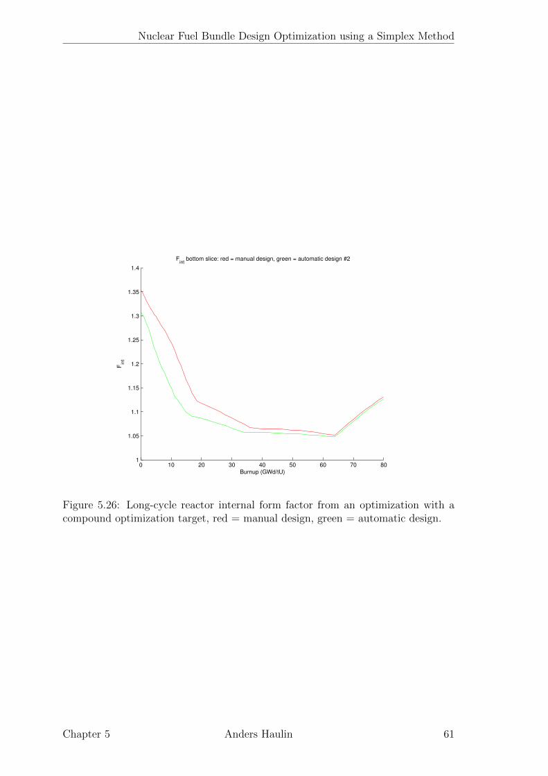
Nuclear Fuel Bundle Design Optimization using a Simplex Method
0 10 20 30 40 50 60 70 801
1.05
1.1
1.15
1.2
1.25
1.3
1.35
1.4
Burnup (GWd/tU)
Fin
t
Fint
bottom slice: red = manual design, green = automatic design #2
Figure 5.26: Long-cycle reactor internal form factor from an optimization with acompound optimization target, red = manual design, green = automatic design.
Chapter 5 Anders Haulin 61

Chapter 6
Discussion
6.1 Simplex framework
6.1.1 Benefits of simplex fuel bundle optimization
In the results section a great number of obstacles hindering ideal implementation ofa bundle optimization program have been presented and focus has been put on theerrors prevalent in the approximations and how to reduce them. A conclusion thathas been drawn is that a linear perturbation optimization scheme such as the oneexamined will be sensitive if it incurs large changes in the design variables (comparedto the reference used as input). The investigations of the optimization scheme haveshown that these errors are hard to combat and that the optimizations may sufferfrom them in an unpredictable manner, sometimes more and sometimes less. Therelative strength of the optimization program has not, however, been found to varybetween reactors in any significant way. That is, longer cycles are harder to optimizeboth manually and automatically.
There are of course great potential benefits to be reaped from automaticallyoptimizing bundle designs functionally: better designs can be found with less timebeing spent on trial-and-error during the bundle design process (a cost estimate forthis is found in Section 6.1.4). It should be noted that automatic optimizationsrequiring a lot of computing time can be beneficial even for nuclear designs wherea skilled engineer could have found an equivalent design in a shorter time; the keyis that the program decreases the total amount of time spent by the engineer onthe bundle design. This requires a good user interface and integration as well asrun-times that are compatible with normal work: i.e. absolutely nothing longer thanovernight optimizations. The prototype optimizer studied and developed on is not,however, at such a stage yet, especially regarding user interface.
Simplex optimization has a beneficial side effect besides actual optimization inthat it can determine limits of possible solutions. If a set of parameters, such aslimits on internal power peaking factor and number of BA rods, are not compatiblethe optimization program will in very short time realize it is infeasible and canceloptimization. This feature is not possible in stochastic optimization and it can helpthe nuclear designer when balancing constraints for bundles to use in a whole coreoptimization.
An optimization of specific concern to the nuclear company was the idea ofoptimizing the BA layout to minimize the total number of Gd rods in a bundle
62
Nuclear Fuel Bundle Design Optimization using a Simplex Method
to improve production, logistics and customs expenses. This optimization was at-tempted by taking a manual design, removing Gd and running a step-1 optimizationon the problem. This approach did however not yield any conclusive results due tothe strict constraints used, lack of time and that a good implementation of thiswould require combination of step 1 and 21.
6.1.2 Simplex method improvements
Several strategies were concocted to improve the simplex framework available at thebeginning of the project. Most of these were investigated in the results section butothers were not possible to implement in the scope of this project.
k∞
Several improvements were attempted for k∞. The symmetric perturbations thatwere implemented proved superior to asymmetric perturbations for the second stepof optimization. Using reference cases with carefully adjusted average enrichmentproved useful for the optimization. In the second step it was seen that large changesin BA concentration affected the optimization accuracy negatively: that the firststep with a correct enrichment profile could better pick BA concentrations whichthe second step did not have to change could therefore improve the accuracy of thesecond step and thus the quality of the optimization.
These improvements were implemented into the optimization framework alongwith more accurate optimization constraints on k∞.
Piecewise linearly constrained variables were interesting to use but made theoptimizations too slow to function. A better implementation of these constraintsor any other part of the simplex implementation (if it increases the speed of theprocess) could make these a viable option for improved accuracy.
A shadow-factor was not implemented in the second optimization step since itwas expected it would also slow down the process further still. A major concernfor step-2 optimizations is, however, that the k∞ profile tends to become shiftedhorizontally from its real value (creating a faulty estimation of b-value). This isthought to be due to an inability to factor in the group effects of several interactingchanges in BA concentration; so a shadow factor accounting for this could be a wayto improve the estimation.
The approximation of k∞ curves is still inaccurate when BA-concentration changesby large amounts, increasing the concentration in many rods will in PHOENIX cal-culations shift the peak burnup (b-value) to higher values but the sum of severalS-matrix elements will not reproduce this effect. A possible explanation is that theextra gadolinium introduced with one perturbation will be quickly burnt out whenall other rods have lower concentrations and the resulting perturbation elements willdiminish quickly beyond the reference design b-value, this does not happen whenseveral rods change together and the result will be that the linear approximationputs the peak at a too low burnup. This situation will reverse if an aggregate BAdecrease is introduced by the optimization.
1One would like to run a BA-placement optimization on many enrichment profiles to find aminimum number of BA rods.
Chapter 6 Anders Haulin 63

Nuclear Fuel Bundle Design Optimization using a Simplex Method
Relative pin power distribution
The accuracy of relative pin power approximation was found to behave in a similarmanner as that of k∞ approximation. BA changes typically induced greater errorsthan enrichment changes, especially when these were clustered. Figure 6.1 showsthe burnup evolution of pin power errors, it is found that these diminish stronglyas BA becomes burnt out. Due to the matrix nature of pin powers it was harder tovisualize the accuracy and implement alternative formulations in CPLEX; thus thebehavior of relative pin powers was not as rigorously studied as that of k∞.
R-factor
The impact of the previously unknown linearization errors of the minimum-functionsin the equations for R have been shown in Section 5.2.3. Allowing this minimumvalue to be explicitly calculated in the simplex optimization proved infeasible as itgreatly increased the optimization time.
Pin power target instead of R-factor approximation The comparison to thedesign obtained by R approximation shows that the pin power deviation minimiza-tion can indeed generate a superior design but at a high cost in calculation time.The reason for this has not been firmly established but the most reasonable idea isthat the optimizer when optimizing an approximation of R can omit more variablesas it identifies the limiting rod at a burnup time, the same not being possible forthe pin power distribution target. It is also striking how summing the deviationsfrom different axial slices drastically increases the calculation time.
Adjusting the target power distribution to account for another constraint onpeak rod power did not improve results. The LHGR constraint was present inall optimizations but including it in the generation of an optimal power profilecould ensure that the optimizer didn’t target a power distribution that one of itsconstraints forbade. That this adjustment didn’t improve results was most likelydue to the change in the optimum power profile was only marginally different inpositions other than the limited rods; all the non-limited positions simply shiftslightly to higher powers and the gains from recalculating are slim (the optimizationonly targets relative pin power values higher than the optimal distribution).
Adjusting the target power distribution to account for another constraint on peakrod power did not improve results. This should be expected since the change in theoptimum power profile resulting from the LHGR constraint is marginally differentin positions other than the limited rods; all the non-limited positions simply shiftslightly to higher powers and the gains from recalculating are slim (the optimizationonly targets relative pin power values higher than the optimal distribution).
Although the pin power distribution target relieves the problem of the minimum-value simplification used in the R-approximation it is not without inaccuracies:the analysis of power-distribution errors in Section 5.2.2 showed that these werereasonably small in the optimizations studied. The calculation of deviations froman optimum does, however, place a much greater demand on accuracy in every rodthan a simple limitation on Fint; which is the normal case of pin power relevance.The R-factor optimization is also specifically targeted at the peak k∞ burnup (sincethis is where the R-factor is most important) where the errors in approximation tendto be substantial. Figure 6.1 shows the maximum pin power errors approximated
64 Chapter 6 Anders Haulin

Nuclear Fuel Bundle Design Optimization using a Simplex Method
by CPLEX in the step 2 optimization leading to the first value in Table 5.4: averageenrichments have changed by less than a 0.02 of a percentage in all three axialslices and about half BA positions increased from 6 to 7 % with the other halfdecreasing from 6 to 5 % so the optimization step has not incurred any large changesin composition. This only emphasizes the need for a deviation optimizer to post-
0 5 10 15 20 25 30 350
0.005
0.01
0.015
0.02
0.025
0.03
Burnup (GWd/tU)
Ab
so
lute
err
or
Max relative pin power errors: blue=bot, red=mid, green=top.
Figure 6.1: Maximum error of pin power estimation in CPLEX approximation. Blue= bottom, red = middle, green = top.
process multiple solutions with low deviations to find the best R-factor as such anoptimization will have uncertainties both in how great the deviation from optimumis and what R-factor this deviation corresponds to.
6.1.3 Feasibility and performance of optimization
The optimizations on real fuel designs show that while it is feasible to use a simplexmethod to optimize fuel bundle designs it is hard to naively use an automatic tooland expect to ”beat” years of experience in fuel design. It is evident however,that such a tool can generate good designs if the problem is approached with someexperience and caution for error in approximations. It also shows that weighingoptimization parameters such as different target functions against each other2 and
2The compound objective used in the optimizations on both the long-cycle and short-cyclereactors were useful in this benchmark as the concern was merely to generate a design that wasas ”good as possible” from several perspectives. The documentation from the manual designs didnot state exactly what constraints had been used in the design, and using the entire Fint-curveof a manual design as a constraint gives an unfair advantage to the manual designs since mostimprovements most come at a (small or large) price in some other parameter or burnup point.When one has hard constraints on parameters, for example a Fint-curve, it is logical to optimizea single variable, usually R, and the constrained variable will most likely border its constraint atexactly one point. Thus a compound objective might be better in these kinds of benchmarks thanin reality, where constraints are hard and ”only” have to be met.
Chapter 6 Anders Haulin 65
Nuclear Fuel Bundle Design Optimization using a Simplex Method
adjusting constraints affect the quality of the solution, thus in no way decreasingthe need for nuclear design expertise.
Impact of poor approximations
It seems obvious that if the objective of an optimization is to optimize a certainproperty and the approximation of this property being used by the optimizationengine is faulty; then the optimized design will also be faulty. However, if the errorimposed by the linearization is virtually consistent for all reasonable designs thenthis error might not limit the optimization tool. After all the goal of the programis to find which is the best design; its actual exact properties can be quickly andaccurately obtained by 2D lattice code calculations.
Examples of errors affecting optimizations The results in Table 5.4 suggestthat different errors in power approximation might have affected the values of R,it is unreasonable that a non-corrected deviation should perform better than onecorrected for axial weighting factor.
After analyzing the results of the long cycle reactor optimization it was foundthat the Excel file entries for the reference enrichments in 4 of 96 positions hadnot been entered correctly. This mishap should be expected to have hampered theperformance of the optimization since it led CPLEX to calculate differences startingfrom incorrect assumptions. This might have contributed slightly to the significantlyless impressive results generated in this optimization, the difference has, however,not been computed. These errors were easily created when using the prototypeframework since there were many manual steps and no safeguards or reminders formistakes.
6.1.4 Recommendations and usage guidelines
Some lessons learned through this thesis will be important to keep in mind for furtherdevelopment of simplex fuel bundle optimization:
• The user can make the optimization much stronger by providing good con-straints and reference designs. These could partially be computer-generated,to account for average enrichment.
• Automating the comparisons of real bundle parameters from the 2D latticecode to the linear approximations used in the simplex program can yield muchbetter and more thorough understanding of what makes the optimizationswork and what doesn’t. This was a step that should have been taken early inthis project but wasn’t due to lack of programming expertize.
• Keeping the errors from above comparisons visible so that all optimizationscan be gauged on their accuracy is important. Including a plugin for externalR-calculations would also be necessary since these aren’t done by the 2D latticecode.
• The time that can be saved with an optimization program is a very importantparameter that hasn’t been accurately estimated during this project, a goodmeasure of this is essential for decision-making.
66 Chapter 6 Anders Haulin
Nuclear Fuel Bundle Design Optimization using a Simplex Method
During the project a consultant has been working in parallel to create a pro-duction version of the optimization program with a new model running on a clusterwith significantly faster and more stable S-matrix generation and data-handling.This program could improve the prospects for automatic optimization greatly andpotentially include some more accurate models. The problems encountered with theR-factor model are important to keep in mind and continued investigation of im-plicit R-calculation from pin power distribution, by someone with good optimizationknowledge, could be a way forward. This would also future-proof the optimizationfor fuel types that do not use XL-correlations and thus have significantly differentR-factor equations.
Cost-benefit analysis
To sum up the recommendations for the optimization project a crude cost-benefitanalysis is useful, the payback time for a project like this is hard to estimate and willpartly depend on whether the optimized fuel bundles will be surpass and be moredesirable than manual designs. In this project the manual designs were however notsurpassed in quality, but it seems viable that an optimizer could eventually designfuel bundles with performance equal to manual designs.
For equivalent fuel a rough calculation of payback time for the nuclear companycan be made with the following assumptions:
• It will take one engineering year to develop an optimizer from idea to pro-duction and support it over its lifetime. Cost of additional software, suchas commercial simplex optimizer license, costs an equivalent 50 engineeringhours.
• Maunual nuclear fuel bundle design generally takes between 4 and 40 hours[24], so a design time of 10 hours for 12-month and 25 hours for 24-monthcycle reactors is assumed.
• A good optimization program can cut the fuel bundle nuclear design time bythree-quarters.
• There are 84 BWRs worldwide [16], assumed to be evenly divided between 12and 24 month cycle operation3.
• The BWR fuel market share of the company is 30%.
• Long-term internal rate of return for large nuclear companies is 5 %[27].
The payback time from time savings alone would then be 15 years. Uncertain-ties are many, such as interest rates and the future size of the BWR market, butthe most important ones are the actual time that will be saved in design and timeneeded to develop and maintain the program. If an automatic optimization tool cre-ates a superior design that can win new customers and increase market share4 thenthe net value of an optimization project quickly becomes very promising. The prof-itability of automatic optimization will, however, not only come from time savings
3If 24-month cycle optimization is assumed to exactly twice as hard as 12-month, the relativeabundance of reactor cycle lengths does not matter.
4Or if not having an automatic optimization tool causes market share to be lost.
Chapter 6 Anders Haulin 67

Nuclear Fuel Bundle Design Optimization using a Simplex Method
and market share (through superior designs) but will depend on how its positive ef-fects are measured. Positive externalities from automatic optimization could includebetter integration with loading pattern optimization, reduced number of Gd con-centrations or enrichments and potentially better customer satisfaction from quickerdesign processes.
6.2 Project evaluation
6.2.1 Goal attainment
The overall goals of the project were: investigating optimizations on nuclear fuelbundles, coming up with and evaluating possible improvements to simplex optimiza-tion code and determining the usefulness and benefits of automatic optimization onnuclear fuel bundle designs. These main tasks have all been thoroughly labored andalthough many results were either expected or erratic there were several notable find-ings that put the light on some unknown difficulties and can enable improvementof the framework. Although the project as a whole has not generated any dramaticbreakthroughs in BWR bundle optimization it has been shown that an optimizationscheme based on linear perturbations can generate useful fuel assembly designs whenthe user is aware of the limits introduced by linearization.
6.2.2 Method used
The method used in the project, of focusing strongly on improvements and errorpatterns in the optimization framework, was a product of the nature of both theproject and the equipment used. The fundamentals of the optimization frameworkwere already in place but poor organization of it (see Figure 6.2) meant that itwas very hard to work with. The focus on sources of various errors was thereforenecessary to being able to evaluate automatic optimization’s performance againstmanual designs. Furthermore the equipment available proved to be a major challengesince licensing issues limited the use of the CPLEX optimizer to a very old versionrunning on a very old computer. This meant that around half the project wasspent not able to do optimizations over full fuel lifetimes since the calculation timebecame far too long. After a long wait a new computer with CPLEX was introducedand the optimizations duly became up to 300 times faster as explained in Chapter4.2.3. A smaller focus on improving optimizer performance could have enabled otherquestions to have been investigated.
6.2.3 Areas for further investigation
The project has borne several ideas that have not been possible to try out but couldvery well be interesting topics of related research.
Stochastic optimization
In Section 1.3.2 a brief explanation of stochastic optimization algorithms was given,it was also argued that these schemes such as these are hampered by the inability
68 Chapter 6 Anders Haulin
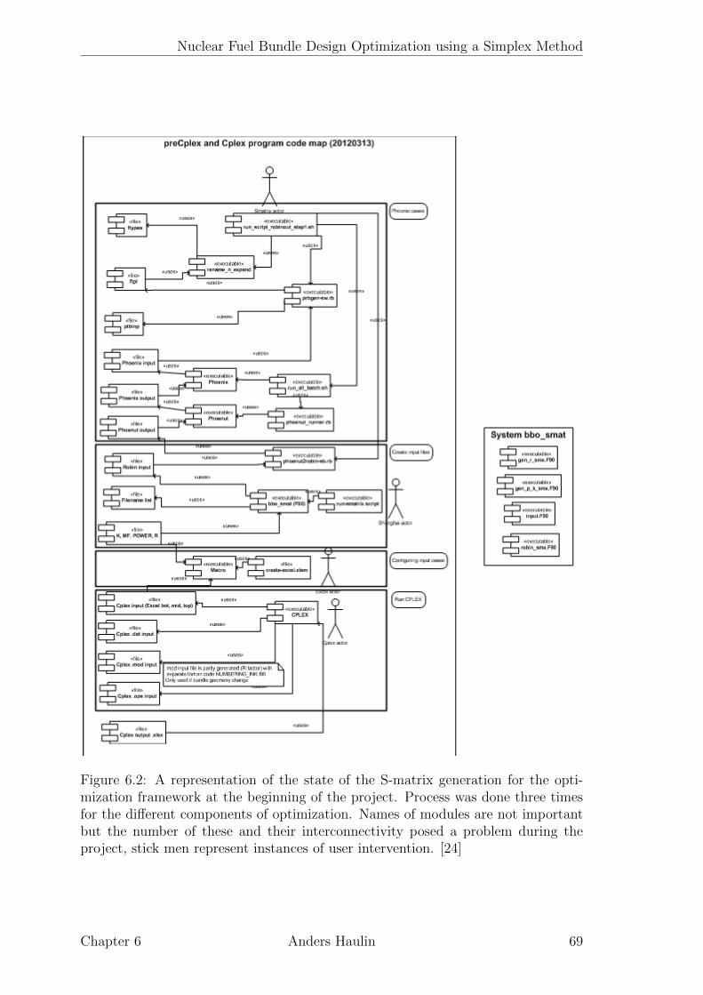
Nuclear Fuel Bundle Design Optimization using a Simplex Method
Figure 6.2: A representation of the state of the S-matrix generation for the opti-mization framework at the beginning of the project. Process was done three timesfor the different components of optimization. Names of modules are not importantbut the number of these and their interconnectivity posed a problem during theproject, stick men represent instances of user intervention. [24]
Chapter 6 Anders Haulin 69

Nuclear Fuel Bundle Design Optimization using a Simplex Method
to estimate if a set of constraints is at all possible to fulfil, or to provide any cluewhether the optimization will run for X seconds or Y hours.
A more thorough investigation including an actual implementation on this prob-lem would, however, be greatly beneficial to understanding the problem and findingthe optimal optimization strategy for BWR bundle designs. The problems surround-ing linearizations of the bundle parameters in Section 5.2 show that there could bea real benefit in calculating bundle parameters such as R and k∞ with 2D latticecodes for every evaluation instead of relying on linearizations. A stochastic approachwould also require a skilled developer to create a good initial population of bundles,as only a minuscule proportion of random designs would meet constraints on param-eters such as k∞. Although a stochastic scheme could work without any ”smart”reference input it might require a very long calculation time to find ”the right track”since evaluating a design takes around 10 seconds in one processor core.
Loading-pattern optimization
Integration into automatic whole core loading-pattern (LP) optimization is currentlyinfeasible, but coupling synergies exist. As was mentioned in the introduction,nuclear fuel optimization most often constitutes two separate steps: fuel bundledesign and core loading pattern, of which only the first is addressed in this project.There are several reasons for the separation of tasks: The problem of deciding whichrod to use at every lattice position in every bundle in a reactor, laterally and axially,is very, very large. The program used to generate perturbation matrices addressesonly 2-D single-bundle physics. A completely different interface would be requiredto generate perturbations on core-level. An interesting topic for research wouldbe to start from a whole core loading pattern problem and use an optimization toprovide constraints on the fresh bundles that should be entered. From there anotheroptimization stage could create those bundles and maximize a whole-core parameter,such as CPR.
6.3 Project conclusion
The project has provided an interesting insight into nuclear power and optimization.The nature of the work has meant that the optimization and programming aspectsof the problem have constituted the majority of the work with the nuclear physicsmainly providing the backdrop. A clearer plan at the onset of the project and greaterawareness and criticism before starting it could have enabled more original work tobe done and clearer conclusions to be drawn.
70 Chapter 6 Anders Haulin
Chapter 7
Bibliography
[1] Status report 97 - Advanced Boiling Water Reactor (ABWR).IAEA, 2011https://aris.iaea.org/sites/..%5CPDF%5CABWR.pdf
Retrieved on 2014-06-07
[2] AP1000 Design Control Document.NRC, unknown yearhttp://www.nrc.gov/reactors/new-reactors/design-cert/ap1000/dcd/
Tier%202/Chapter%205/5-1_r15.pdf
Retrieved on 2014-06-07
[3] Nuclear Data for safeguards.IAEA unknown yearhttps://www-nds.iaea.org/sgnucdat/a6.htm
Retrieved on 2014-06-08
[4] Zoran Stosic, 1999Study on Thermal Performance and Marrgins of BWR Fuel Elements.7th International Conference on Nuclear Engineering.http://www.jsme.or.jp/monograph/pes/1999/ICONE7/PAPERS/TRACK07/
FP7283.PDF
Retrieved on 2014-06-08
[5] Imagine the UniverseDr. James C. Lochner2005http://imagine.gsfc.nasa.gov/docs/teachers/elements/imagine/
Cosmic.pdf
Page 16.Retrieved on 2014-06-08.
[6] Chart of NuclidesNational Nuclear Data Center, Brookhaven National Laboratory.http://www.nndc.bnl.gov/chart/help/index.jsp#colorcode
Retrieved on 2014-06-08.
[7] Uranium 2011: Resources, Production and Demand. OECD & IAEA2012
71
Nuclear Fuel Bundle Design Optimization using a Simplex Method
ISBN 978-92-64-17803-8http://www.oecd-nea.org/ndd/reports/2012/
uranium-2011-exec-summary.pdf
[8] 17x17 Next Generation Fuel (17x17 NGF) Reference Core ReportBarsic, Conner et. al.March 2008.http://pbadupws.nrc.gov/docs/ML0810/ML081010603.pdf
Retrived on 2014-06-09.
[9] Upgrade of the FRIGG test loop for BWR fuel assembliesOlov NylundABB Review 6/1997http://www05.abb.com/global/scot/scot271.nsf/veritydisplay/
a3a21d156256c229c1256ebd00308051/$File/47-53%20ENG%209706.pdf
Retrived on 2014-06-09.
[10] Fuel Design Evaluation for ATRIUM TM 1OXM BWR Reload Fuel AREVANP Inc.Submitted to the NRC April 2010http://pbadupws.nrc.gov/docs/ML1011/ML101100643.pdf
[11] Westinghouse 2003.Westinghouse BWR ECCS Evaluation Model: Supplement 3 to Code Descrip-tion, Qualification and Application to SVEA-96 Optima2 Fuel. Page 14.http://pbadupws.nrc.gov/docs/ML0312/ML031220224.pdf
Retrieved on 2014-06-09
[12] Personal Source: Sven-Birger JohannessonPrincipal Engineer, BWR Core DesignJune 2014.
[13] Butler, Walter R.GENERAL ELECTRIC BWR THERMAL ANALYSIS BASIS (GETAB):DATA, CORRELATION AND DESIGN APPLICATIONSubmitted to NRC September 1974http://pbadupws.nrc.gov/docs/ML1022/ML102290144.pdf
[14] Yamamoto, A.A Quantitative Comparison of Loading Pattern Optimization Methods for In-Core Fuel Management of PWRJournal of NUCLEAR SCIENCE and TECHNOLOGY, Vol. 34, No. 4, p. 339-347 (April 1997)
[15] Asgari et al.Application of the N-StreamingSM Concept to Peach Bottom 2 Cycle 17PHYSOR-2006, ANS Topical Meeting on Reactor Physicshttp://mathematicsandcomputation.cowhosting.net/PHYSOR-2006/C154.
Retrieved on 2014-06-09
72 Chapter 7 Anders Haulin

Nuclear Fuel Bundle Design Optimization using a Simplex Method
[16] Euronuclear.orgNuclear power plants, world-wide, reactor typesUpdated 18 January 2013.http://www.euronuclear.org/info/encyclopedia/n/npp-reactor-types.
htm
Retrieved on 2014-06-09.
[17] Kim, T.K. & Kim, C.H. Mixed Integer-Programming for Pressurised WaterReactor Fuel-Loading-Pattern OptimizationNuclear Science and Engineering: 127, 346-357 (1997)
[18] US Patent 20040220787 A1Russell, W.2003Method and arrangement for developing core loading patterns in nuclear reac-tors
[19] US Patent 7224761 B2Popa, F.2007Method and algorithm for searching and optimizing nuclear reactor core loadingpatterns
[20] Personal Source: Fredrik WaldemarssonEngineer, Thermal HydraulicsInterviewed 2014-07-11.
[21] Leinweber, G. et. al. Neutron Capture and Total Cross-Section Measurementsand Resonance Parameters of GadoliniumNuclear Science and Engineering: 154, 261–279 (2006)http://devinbarry.com/pubs/Journal%20Articles/NSE_154_Gd.pdf
[22] Kenneth S. KraneIntroductory Nuclear PhysicsWiley, 1987
[23] John R. Lamarsh & Anthony J. BarattaIntroduction to Nuclear EngineeringPrentice Hall, 2001
[24] Personal Source: Simon Walve, M.Sc. Senior Engineer BWR Core Design2012
[25] Personal Source: Mikael Call, Ph.D. Senior software developer.2014
[26] Sveriges MekanstandardiseringKarnenergiordlista, Glossary of nuclear energyTekniska nomenklaturcentralen, 1990
[27] Thomas PikettyCapital in the Twenty-First CenturyThe Belknap Press, 2014
Chapter Anders Haulin 73
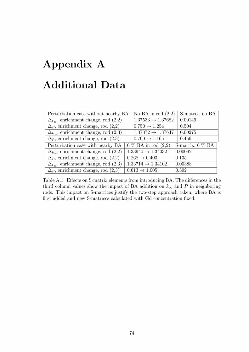
Appendix A
Additional Data
Perturbation case without nearby BA No BA in rod (2,2) S-matrix, no BA∆k∞ , enrichment change, rod (2,2) 1.37533→ 1.37682 0.00149∆P , enrichment change, rod (2,2) 0.750→ 1.254 0.504∆k∞ , enrichment change, rod (2,3) 1.37372→ 1.37647 0.00275∆P , enrichment change, rod (2,3) 0.709→ 1.165 0.456
Perturbation case with nearby BA 6 % BA in rod (2,2) S-matrix, 6 % BA∆k∞ , enrichment change, rod (2,2) 1.33940→ 1.34032 0.00092∆P , enrichment change, rod (2,2) 0.268→ 0.403 0.135∆k∞ , enrichment change, rod (2,3) 1.33714→ 1.34102 0.00388∆P , enrichment change, rod (2,3) 0.613→ 1.005 0.392
Table A.1: Effects on S-matrix elements from introducing BA. The differences in thethird column values show the impact of BA addition on k∞ and P in neighboringrods. This impact on S-matrices justify the two-step approach taken, where BA isfirst added and new S-matrices calculated with Gd concentration fixed.
74

Nuclear Fuel Bundle Design Optimization using a Simplex Method
0 10 20 30 40 50 601.02
1.04
1.06
1.08
1.1
1.12
1.14
1.16
1.18
1.2
1.22
Burnup (GWd/tU)
Fin
t
Fint
middle slice, Red = Manual design , Green = Automatic
Figure A.1: Short-cycle reactor middle slice maximum relative pin power, red =manual design, green = automatic design. In the middle slice the automatic op-timization performs better than the manual design throughout most of the cycle,better than bottom slice comparison shown in Figure 5.20.
Chapter A Anders Haulin 75

Nuclear Fuel Bundle Design Optimization using a Simplex Method
0 10 20 30 40 50 601
1.05
1.1
1.15
1.2
1.25
Burnup (GWd/tU)
Fin
t
Fint
top slice, Red = Manual design , Green = Automatic
Figure A.2: Short-cycle reactor top slice maximum relative pin power, red = manualdesign, green = automatic design. In the middle slice the automatic optimizationperforms worse than the manual design throughout most of the cycle, especiallyearly in the cycle. The manual design, however, had excess margin so together withFigures 5.20 and A.1 this shows that gains in automatic optimization performancecan come from better using all available margins to improve performance in the”worst” rod segment.
Bottom Slice, 0 GWd/tU
-0.014 0.002 0.006 0.000 0.001 0.001 0.000 0.005 0.002 -0.014
0.002 -0.003 0.000 -0.002 0.003 0.003 -0.003 0.000 0.000 0.003
0.006 0.000 0.002 0.002 0.000 0.000 0.003 0.001 0.000 0.006
0.000 -0.002 0.002 -0.001 -0.003 -0.004 -0.002 0.003 -0.001 0.001
0.001 0.003 0.000 -0.003 0.000 0.000 0.000 0.000 0.004 0.001
0.001 0.002 0.000 -0.004 0.000 0.000 0.001 0.000 0.003 0.002
0.000 -0.003 0.002 -0.002 0.000 0.001 -0.004 0.002 -0.001 0.000
0.005 0.000 -0.001 0.003 0.000 0.000 0.002 0.002 0.001 0.005
0.002 -0.002 0.000 -0.003 0.003 0.003 -0.002 0.000 -0.003 0.001
-0.014 0.002 0.006 0.000 0.000 0.001 0.000 0.005 0.001 -0.015
Figure A.3: Pin power relative errors, Figure 5.7 adjusted for power in rods, after astep-2 optimization. All errors are below 2 %.
76 Chapter A Anders Haulin
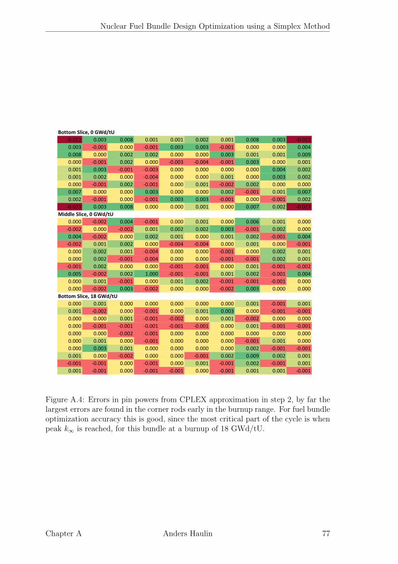
Nuclear Fuel Bundle Design Optimization using a Simplex Method
Bottom Slice, 0 GWd/tU
-0.022 0.003 0.008 0.001 0.001 0.002 0.001 0.008 0.003 -0.022
0.003 -0.001 0.000 -0.001 0.003 0.003 -0.001 0.000 0.000 0.004
0.008 0.000 0.002 0.002 0.000 0.000 0.003 0.001 0.001 0.009
0.000 -0.001 0.002 0.000 -0.003 -0.004 -0.001 0.003 0.000 0.001
0.001 0.003 -0.001 -0.003 0.000 0.000 0.000 0.000 0.004 0.002
0.001 0.002 0.000 -0.004 0.000 0.000 0.001 0.000 0.003 0.002
0.000 -0.001 0.002 -0.001 0.000 0.001 -0.002 0.002 0.000 0.000
0.007 0.000 0.000 0.003 0.000 0.000 0.002 -0.001 0.001 0.007
0.002 -0.001 0.000 -0.001 0.003 0.003 -0.001 0.000 -0.001 0.002
-0.023 0.003 0.008 0.000 0.000 0.001 0.000 0.007 0.002 -0.023
Middle Slice, 0 GWd/tU
0.000 -0.002 0.004 -0.001 0.000 0.001 0.000 0.006 0.001 0.000
-0.002 0.000 -0.002 0.001 0.002 0.002 0.003 -0.001 0.002 0.000
0.004 -0.002 0.000 0.002 0.001 0.000 0.001 0.002 -0.001 0.004
-0.002 0.001 0.002 0.000 -0.004 -0.004 0.000 0.001 0.000 -0.001
0.000 0.002 0.001 -0.004 0.000 0.000 -0.001 0.000 0.002 0.001
0.000 0.002 -0.001 -0.004 0.000 0.000 -0.001 -0.001 0.002 0.001
-0.001 0.002 0.000 0.000 -0.001 -0.001 0.000 0.001 -0.001 -0.002
0.005 -0.002 0.002 1.000 -0.001 -0.001 0.001 0.002 -0.001 0.004
0.000 0.001 -0.001 0.000 0.001 0.002 -0.001 -0.001 -0.001 0.000
0.000 -0.002 0.003 -0.002 0.000 0.000 -0.002 0.003 0.000 0.000
Bottom Slice, 18 GWd/tU
0.000 0.001 0.000 0.000 0.000 0.000 0.000 0.001 -0.001 0.001
0.001 -0.002 0.000 -0.001 0.000 0.001 0.003 0.000 -0.001 -0.001
0.000 0.000 0.001 -0.001 -0.002 0.000 0.001 -0.002 0.000 0.000
0.000 -0.001 -0.001 -0.001 -0.001 -0.001 0.000 0.001 -0.001 -0.001
0.000 0.000 -0.002 -0.001 0.000 0.000 0.000 0.000 0.000 0.000
0.000 0.001 0.000 -0.001 0.000 0.000 0.000 -0.001 0.001 0.000
0.000 0.003 0.001 0.000 0.000 0.000 0.000 0.002 -0.001 -0.001
0.001 0.000 -0.002 0.000 0.000 -0.001 0.002 0.009 0.002 0.001
-0.001 -0.001 0.000 -0.001 0.000 0.001 -0.001 0.002 -0.001 0.001
0.001 -0.001 0.000 -0.001 -0.001 0.000 -0.001 0.001 0.001 -0.001
Figure A.4: Errors in pin powers from CPLEX approximation in step 2, by far thelargest errors are found in the corner rods early in the burnup range. For fuel bundleoptimization accuracy this is good, since the most critical part of the cycle is whenpeak k∞ is reached, for this bundle at a burnup of 18 GWd/tU.
Chapter A Anders Haulin 77


