Noname manuscript No.(will be inserted by the editor)

Numerical continuation analysis of a three-dimensional aircraftmain landing gear mechanism

J. A. C. Knowles · B. Krauskopf · M. Lowenberg

Received: date / Accepted: date

Abstract A method of investigating quasi-static land-ing gear mechanisms is presented and applied to a three-dimensional aircraft main landing gear mechanism model.The model has 19 static equilibrium equations and 20equations describing the geometric constraints in themechanism. In the spirit of bifurcation analysis, solu-tions to these 39 steady-state equations are found andtracked, or continued, numerically in parameters of in-terest. A design case-study is performed on the land-ing gear actuator position to demonstrate the poten-tial relevance of the method for industrial applications.The trade-off between maximal efficiency and peak ac-tuator force reduction when positioning the actuatoris investigated. It is shown that the problem formula-tion is very flexible and allows actuator force, lengthand efficiency information to be obtained from a sin-gle numerical continuation computation with minimaldata post-processing. The study suggests that numeri-cal continuation analysis has potential for investigatingeven more complex landing gear mechanisms, such asthose with more than one sidestay.

Keywords Landing Gear · Bifurcation analysis ·Numerical continuation

The research of J. A. C. Knowles was supported by an Engi-neering and Physical Sciences research council CASE awardin collaboration with Airbus

J. A. C. KnowlesFaculty of Engineering, Queen’s Building, University Walk,Bristol, BS8 1TR, UK

B. KrauskopfDepartment of Mathematics, The University of Auckland,Private Bag 92019, Auckland 1142, New Zealand

M. LowenbergFaculty of Engineering, Queen’s Building, University Walk,Bristol, BS8 1TR, UK

1 Introduction

The landing gears on an aircraft are used to transferground loads during take-off, landing and taxiing, intothe structural elements of the fuselage and wing. Untilthe late 1920s, landing gears were structural elementsthat either remained attached to the aircraft, protrud-ing during flight as on the ground, or were ditched upontake-off to reduce weight and drag but leaving the pilotto await an uncomfortable landing [1]. These rather in-elegant solutions were soon superceded by retractablelanding gears, which offered the drag reduction benefitsof the detachable gears alongside the landing comfortassociated with keeping the gears attached to the air-craft, for the price of a (small) weight penalty.

Current civil airliners all use retractable landinggear mechanisms for their nose landing gear (NLG) andmain landing gears (MLG). These designs vary from air-craft to aircraft, but there are some standard features oflanding gear mechanisms that are present on all moderncivil airliners. For a sketch of a typical single-sidestayMLG configuration see Figure 1. The main structuralelement of the landing gear is the shock strut. It isresponsible for absorbing vertical loads on touchdown,and for reducing the vibrations experienced in the cabinwhen the aircraft is in motion on the ground. One endof the shock strut is connected to the wing, with theopposite end holding the wheel assembly. The shockstrut is supported by a sidestay when in the deployedposition, which transfers loads acting perpendicular tothe shock strut axis into the airframe. As the mecha-nism must be able to move between the deployed andretracted states, this sidestay is required to fold; thesidestay therefore comprises an upper sidestay link at-tached to the airframe at one end, joined to a lowersidestay link attached to the shock strut. At or near

2 J. A. C. Knowles et al.

the folding point between the upper and lower sidestaylinks, a pair of locklinks are used to fix the two sidestaylinks to be in line when the MLG is deployed. Theselocklinks keep the landing gear locked in the deployedposition, and they must be unlocked before the retrac-tion cycle commences.

For some landing gears, the retraction mechanismis able to operate in a fixed plane; NLG mechanismsare typical examples of such planar landing gear mecha-nisms. These landing gears can be modelled mathemat-ically in a planar co-ordinate system, reducing the com-plexity of their mathematical description. Many land-ing gears however, and in particular the MLG on prac-tically all current civil airliners, do not retract in afixed plane. These landing gears are stowed in the wingroot/fuselage intersection, where limited stowage heightwithin the wing prohibits the possibility of retractingin a planer manner. It is therefore necessary for thesidestays and locklinks of the MLG to rotate out ofthe retraction plane whilst the gear retracts or deploys.This allows the mechanism to lie flat in the body of theaircraft when retracted, requiring a minimal amount ofspace to stow the gear. The three-dimensional natureof the MLG mechanism implies that the mechanismcannot be described within a single planar co-ordinatesystem; hence the approach adopted here is to modelthe mechanism in terms of two rotational planes – aglobal plane in which the shock strut rotates and a lo-cal plane in which the sidestays and locklinks rotate;the latter plane itself moves as a function of the shockstrut position.

Irrespective of how the landing gear mechanism op-erates, it requires some form of energy input to movebetween the deployed and retracted state. This energyis provided by the retraction actuator. The retractionactuator must achieve a smooth transition between thedeployed and retracted states to maximise the struc-tural life of the aircraft and maintain passenger com-fort, whilst operating as efficiently as possible withoutadding an excessive amount of weight to the aircraft. Itmust also provide enough energy to overcome the land-ing gear weight and any aerodynamic forces (such asdrag) which may be working against the retracting gear.In the NLG previously considered in [2], both aerody-namic drag and structural weight worked in the NGLretraction plane in a manner that aided the actuatormotion when extending the gear, but opposed the re-traction motion. For a MLG the aerodynamic drag doesnot have such a large effect on the landing gear exten-sion and retraction, because a MLG main strut usuallymoves in a plane perpendicular to the onset flow. Thismeans that when the aircraft is flying directly into theflow with zero sideslip there is no drag force acting in

the MLG shock strut retraction plane. On the otherhand, when the aircraft is sideslipping during landingor takeoff, the drag component in the retraction planemay either aid or oppose a retracting MLG (dependingon which direction the aircraft is sideslipping).

The challenge of designing a landing gear can betackled in different ways, each chosen depending onvarying requirement levels of complexity and accuracy.Geometric analysis methods are often used during pre-liminary design to size the landing gear [3], whilst fulldynamic multibody simulations are generally used formore detailed design purposes later on in the designprocess. There is, however, largely an absence of in-termediate level methods in the literature on landinggear modelling: when analytical methods become toocomplicated to be implemented easily, the aircraft de-signer will generally resort to using dynamic simula-tions, creating and analysing a model with conventionalindustrial-standard multi-body simulation software suchas ADAMS or Dymola. Whilst these models have thecapacity to provide very accurate replications of reality,the time requirements to create, validate and run thesemodels suggests that there is considerable potential forcomplementary analysis approaches.

The complementary approach presented here makesuse of concepts from the theory of dynamical systems;see [4–6] for background information. Several recent ap-plications of dynamical systems methods have demon-strated the advantages that they can offer in an aerospacecontext; this includes the analysis of aircraft ground dy-namics [7,8], the study of nose landing gear shimmy [9]and NLG mechanism modelling [2]. To be able to usethese dynamical systems methods for analysing land-ing gear mechanisms, the mechanism configuration andinternal force distribution is formulated as a system ofcoupled equations, which are inherently nonlinear dueto various geometric constraints. The steady-state solu-tions of these equations can then be found and followed,or continued, in parameters of interest with standardnumerical continuation software, such as AUTO [10]or, as is used for this research, the Dynamical SystemsToolbox extension for MATLAB [11]. A particular ad-vantage of this coupled-equation approach is that solu-tions can be continued in phase and parameter spacewithout the need to reformulate the governing equa-tions as a function of specific parameters under consid-eration. This approach to the equation formulation alsoallows for a convenient analysis of different landing gearconfigurations, as the model is fully parameterised. Theadvantage of this over traditional simulations is that thesame model (with new parameter values) can be usedfor any number of different landing gear configurations.

Numerical continuation analysis of a three-dimensional aircraft main landing gear mechanism 3

Fig. 1: Plan views of the single sidestay MLG; axes denote the positive directions of the global (X,Y ,Z) co-ordinatesystem, whose origin is at the shock strut attachment point O.

The method is demonstrated with a case study intothe effect of the landing gear retraction/extension ac-tuator placement on actuator performance. Three mea-sures of actuator performance are considered: peak force,efficiency and actuator length change. All of these mea-sures are obtained with minimal post-processing of thenumerical continuation data and can, hence, be used di-rectly to inform design decisions. These results are com-pared to those obtained analytically for a simplified ge-ometric actuator model. A general agreement betweenthe two sets of results is demonstrated, which validatesthe numerical continuation study, but the limitations ofthe geometric model highlight the scope and suitabilityof numerical continuation as a tool to analyse complexlanding gear mechanisms.

The paper is organised as follows. Section 2 de-scribes the landing gear model used in the continua-tion analysis, leading on to the retraction actuator casestudy investigation of this model presented in Section 3.The analysis of the simplified geometric model is pre-sented in Secton 3.6, and future avenues for MLG mod-elling and analysis can be found in Section 4.

2 Single-Sidestay MLG Mechanism Model

The single sidestay MLG considered here consists offive links; they are assumed to be rigid bodies with uni-formly distributed mass along their lengths. Each link,Li, is connected to another link or the aircraft structurevia rotational joints; joints C, D, E and O are planarjoints, whilst joints A and B are spherical joints that

allow connected bodies to rotate about the joint freelyin three-dimensions. Figure 1 shows the global land-ing gear co-ordinate system, with capital letters usedthroughout to denote global position co-ordinates androtations. For simplicity, the X-axis is defined as theshock strut rotation axis, with the shock strut rotationjoint at the global co-ordinate origin point O. The gearretracts in the positive Y -direction and the Z-axis isaligned with the global gravity vector, positive down.The landing gear shock strut rotation is therefore con-fined to the global (Y, Z)-plane throughout the retrac-tion cycle. Note that this choice of global co-ordinatesystem is chosen to align closely with the convention foraircraft body axes, where the X-axis is along the bodyof the aircraft (roll axis) positive from c/g to nose, theZ-axis (yaw axis) positive down and the Y -axis (pitchaxis) defined to create a right-handed co-ordinate sys-tem. These co-ordinates were chosen to facilitate trans-forming landing gear points given in aircraft body axesto the global co-ordinates used here.

The local sidestay rotation plane is defined by pointsA, O and B from Figure 1. Vector OA is assumed fixedin the global co-ordinate system, and vector OB is de-fined as a function of the global shock strut rotationangle θ1 because points O and B are fixed relative tothe shock strut. The normal vector to the sidestay ro-tation plane is therefore

n = OB ×OA . (1)

The sidestay local co-ordinate system can now bedefined with a rotation matrix T about the global origin

4 J. A. C. Knowles et al.

point O, that aligns the local x-axis with n by a rotationover α about the global Y -axis followed by a rotationthrough β about the intermediate z-axis:

T =

cosβ cosα − sinβ cosβ sinαsinβ cosα cosβ sinβ sinα− sinα 0 cosα

. (2)

Lower case letters are used throughout to denote lo-cal position co-ordinates and rotations, such that localand global co-ordinates can be related by

xyz

= T

XYZ

. (3)

The (y, z)-plane in the transformed co-ordinates isthe sidestay rotation plane, obtained by applying thetransformation matrix T to the global co-ordinates. Thesidestays (links L2 and L3) and locklinks (links L4 andL5) are constrained to rotate in this transformed plane,and as such their geometric constraints are formulatedin local co-ordinates. The shock strut (link L1) is con-strained to rotate about the global X-axis, described interms of global co-ordinates.

The equations are formulated by considering eachlink Li within the mechanism as an individual rigidbody in static equilibrium. This method has been usedin previous work to study planar mechanisms, and wasshown to provide equivalent results to those obtainedwith a multibody dynamic simulation software pack-age [2]. The challenge for a three-dimensional land-ing gear is to provide a convenient formulation andimplementation of the planar constraints between thesidestays and locklinks in three-dimensional space. Thesolution adopted here is to constrain the sidestays to liein a local plane defined by the main fitting and sidestayattachment point position. The geometric constraintscan then be implemented in the same way as for the pla-nar mechanisms in previous work, with the additionalconstraint that the x-co-ordinate of the transformed el-ements be zero throughout.

2.1 Link description and co-ordinate systems

Figure 2 depicts the general naming convention used foreach link within the landing gear mechanism in localco-ordinates. Each link is described in terms of sevenelements, Li = Xi, Yi, Zi, n, θi, Li,mi, where:

– Li is the ith link;– Xi, Yi, Zi are the global Cartesian co-ordinates which

describe the position of Li’s centre of gravity (cg);

.

.

!2

(x2, y2, z2)

!3

(x3, y3, z3)

!1

(x1, y1, z1)

!4

(x4, y4, z4)

!5

(x5, y5, z5)

z

y

!i

Fig. 2: Mechanism expressed in local co-ordinates, asviewed along the normal vector to the sidestay plane.

– n is the normal vector to Li’s plane of rotation, i.e.out of the page in Figure 2;

– θi is the local rotation of Li relative to the localy-axis1;

– Li is the length of Li;– mi is the mass of Li, assumed to be evenly dis-

tributed along Li.Each link is also acted upon by several forces. These

forces can be expressed in global or local co-ordinateswhich are related via the transformation matrix T as:

F xF yF z

= T

FXFYFZ

. (4)

The left-hand side of Equation (4) is the local (x,y,z)projection of the given force, with the symbol F usedto distinguish the force as being in local co-ordinates;the right-hand side of the equation contains the global

1 For the main strut L1 a global rotation Θ1 is used to de-fine the link. The corresponding local rotation θ1 is a functionof Θ1

Numerical continuation analysis of a three-dimensional aircraft main landing gear mechanism 5

.

.

−101

0

1

2

3

−3

−2

−1

0

1

−1

0

10 1 2 3

0 1 2 3−3

−2

−1

0

1

(a)

!Z(m)

Y (m)

X (m)

(b)X(m)

Y (m)

(c)!Z(m)

Y (m)

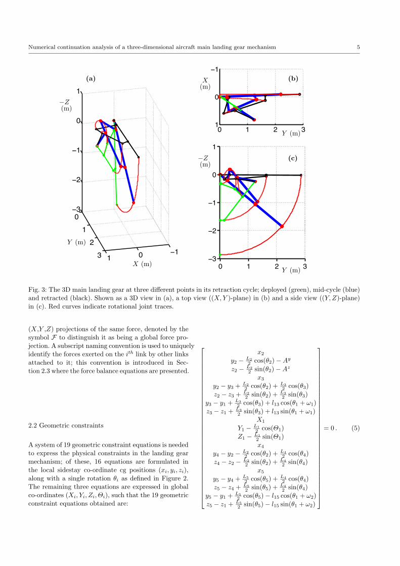
Fig. 3: The 3D main landing gear at three different points in its retraction cycle; deployed (green), mid-cycle (blue)and retracted (black). Shown as a 3D view in (a), a top view ((X,Y )-plane) in (b) and a side view ((Y,Z)-plane)in (c). Red curves indicate rotational joint traces.

(X,Y ,Z) projections of the same force, denoted by thesymbol F to distinguish it as being a global force pro-jection. A subscript naming convention is used to uniquelyidentify the forces exerted on the ith link by other linksattached to it; this convention is introduced in Sec-tion 2.3 where the force balance equations are presented.

2.2 Geometric constraints

A system of 19 geometric constraint equations is neededto express the physical constraints in the landing gearmechanism; of these, 16 equations are formulated inthe local sidestay co-ordinate cg positions (xi, yi, zi),along with a single rotation θi as defined in Figure 2.The remaining three equations are expressed in globalco-ordinates (Xi, Yi, Zi, Θi), such that the 19 geometricconstraint equations obtained are:

x2

y2 − L22 cos(θ2)−Ay

z2 − L22 sin(θ2)−Az

x3

y2 − y3 + L22 cos(θ2) + L3

2 cos(θ3)z2 − z3 + L2

2 sin(θ2) + L32 sin(θ3)

y3 − y1 + L32 cos(θ3) + l13 cos(θ1 + ω1)

z3 − z1 + L32 sin(θ3) + l13 sin(θ1 + ω1)

X1

Y1 − L12 cos(Θ1)

Z1 − L12 sin(Θ1)x4

y4 − y2 − L22 cos(θ2) + L4

2 cos(θ4)z4 − z2 − L2

2 sin(θ2) + L42 sin(θ4)

x5

y5 − y4 + L52 cos(θ5) + L4

2 cos(θ4)z5 − z4 + L5

2 sin(θ5) + L42 sin(θ4)

y5 − y1 + L52 cos(θ5)− l15 cos(θ1 + ω2)

z5 − z1 + L52 sin(θ5)− l15 sin(θ1 + ω2)

= 0 . (5)

6 J. A. C. Knowles et al.

Here Ay and Az are the local co-ordinate y- and z-components of the sidestay attachment point (point Ain Figure 1), l13 and l15 are the lengths from the shockstrut cg to the adjoining ends of links L3 and L5 respec-tively, and ω1 and ω2 are the angles l13 and l15 makewith the shock strut centreline (in local co-ordinates).All other symbols follow the naming convention as de-scribed in Section 2.1, with capital letters indicatingglobal co-ordinates and lower cases indicating local co-ordinates.

The above system of 19 equations is described interms of 20 link positional states (Xi,Yi,Zi,θi for i ∈Z = [1, 5]); therefore, if one of the 20 states is speci-fied, the other 19 states can be determined uniquely.This can be used to plot the relation between differ-ent positional states, or the states can be used to plotthe configuration of the landing gear at various pointsthroughout the retraction cycle. Figure 3 was createdfrom a continuation run using just the geometric statesand constraints from Equation (5). It shows the land-ing gear in three positions; deployed (but unlocked)in green, semi-retracted (Θ1 = 40) in blue and fullyretracted in black. In Figure 3(a) the landing gear isviewed in 3D. Dots are used to indicate the mechanismjoint positions for each of the links, with red lines trac-ing out the joint positions for the five links as the gearmoves from the deployed to retracted state.

The two projections in Figure 3(b) and 3(c) providea sense of the three-dimensional nature of the mecha-nism. Considering the deployed gear depicted in green,all of the links can be viewed clearly in the (Y, Z) planeshown in Figure 3(c), but looking down on the gear inFigure 3(b) the sidestay and locklinks appear to be ontop of each other. This is because the shock strut sits(approximately) vertically in the deployed position, sothe sidestay rotation plane (which is a function of shockstrut angle) is also vertical when the gear is deployed.As the gear retracts, the sidestay plane rotates so that,when the gear is viewed around the midway point inthe retraction cycle (blue gear, in Figure 3), all linksare clearly visible in projections Figure 3(b) and 3(c).As the landing gear retracts further, the sidestay planebecomes more horizontal until Θ1 = 10 when the linksend up in their ‘most horizontal’ state (i.e. they areviewed as a single line in a side view). In the fully re-tracted state for Θ1 = 0 (the black gear in Figure 3)the sidestay plane has rotated more than 90 from thedeployed state so the gear does not appear as a singleline in Figure 3(c). This large rotation that the sidestayplane experiences is the main reason why the red jointtraces between the sidestay links and locklinks in Fig-ure 3 are non-circular.

2.3 Force and Moment Equilibrium Equations

The 19 geometric constraints are supplemented with asecond set of 19 equations that describe the force andmoment equilibrium necessary for the gear to be in asteady-state. For the whole MLG to be in equilibrium,each of the five links must be in force and moment equi-librium and the joints must be in force equilibrium. Thegeneral equilibrium cases are discussed below.

.

.

A

F y2;RA

F z2;RA

CF y2;3,4

F z2;3,4

L2

!2

F y2;g

F z2;g

Fig. 4: Free-body diagram of link L2 in local co-ordinates.

Figure 4 shows a free-body diagram for the uppersidestay link L2 in the sidestay rotation plane. It isrepresentative of all links in local co-ordinates, that is,for the lower sidestay link (L3) and the locklinks (L4

and L5); the specific case for the shock strut is con-sidered later. In the general case, there are two typesof forces which act on the link: the externally createdforces due to gravity or drag, and the resultant inter-nal forces transferred by links joined to link L2. Theseforces are denoted by Fi;∗ in the general case, wherethe subscript i denotes the link number that the forceis acting on and the subscript ∗ denotes the elementexerting that force on Li which can be:

– the in-plane gravitational force acting on the body– mig,

– the internal force applied by an adjoining link(s) –Fi;∗ – where the link number appears in place of thesymbol ∗,

– the internal force between the strut and the aircraftbody, either RA for the reaction force at point A orRO for the reaction force at point O.

Numerical continuation analysis of a three-dimensional aircraft main landing gear mechanism 7

The superscripts denote the component of that forcein the local co-ordinate directions. From Figure 4, theforce denoted by F y2;RA can therefore be interpreted asbeing the local y-component of the force exerted on L2

by the aircraft body at point A, whereas F z2;3,4 is thelocal z-component of the force exerted on L2 by theadjoining links, L3 and L4.

Within the sidestay plane, for an arbitrary link Lito be in static equilibrium the sum of the forces actingon the link must equal zero. Using the notation conven-tions introduced before, this means that:

∑∗F yi;∗ = 0 , (6a)

∑∗F zi;∗ = 0 . (6b)

The forces depicted in Figure 4 are acting in thechosen positive direction, which aligns with the positivelocal (y, z) co-ordinate directions. For the specific caseof L2, Equations (6a)–(6b) become:

∑∗F y2;∗ = F y2;RA + F y2;g + F y2;3,4 = 0 , (7a)

∑∗F z2;∗ = F z2;RA + F z2;g + F z2;3,4 = 0 . (7b)

The sum of the moments about any given point Palong the link must also be zero. Since the moments arecreated by forces, it is convenient to use a similar sub-script naming convention as used above for the forcesthemselves, with a slight change in the meaning of thesuperscript: it now denotes the point in the sidestayrotation plane about which moments are taken, andlength lPi;∗ is the moment arm of force Fi;∗. The gen-eral expression for this moment equilibrium conditiontherefore is:

∑∗MPi;∗ = lPi;∗Fi;∗ = 0 . (8)

Point P can be chosen arbitrarily, but to simplifythe moment equilibrium expression as much as possibleP is chosen at joint A for link 2 (see Figure 4), so thatthe forces acting at that end of the link do not have tobe included in the moment equilibrium expression.

Counter-clockwise moments are taken to be posi-tive, as this reflects the positive rotation sign conven-tion used in the local co-ordinate system. As the linksare assumed to be homogenous, the gravitational forceacts at the geometric midpoint of the ith link; this leads

to the following expression for the moment equilibriumequation of L2:

∑∗M

A1;∗ = L2 sin(θ2)(F y2;3,4 + 1

2Fy2;g)

+L2 cos(θ2)(F z2;3,4 + 12F

z2;g) = 0 .

(9)

Further constraints are applied by enforcing the ‘equi-librium of joints’ condition in between joined elements.For L2, no links are joined at point A, but both L3

and L4 are joined to L2 at point C so the sum of allinternal joint forces at point C must be zero for themechanism to be in static equilibrium. The resultingforce equilibrium equations at joint C are therefore:

F y2;3,4 + F y3;2,4 + F y4;2,3 = 0 , (10a)

F z2;3,4 + F z3;2,4 + F z4;2,3 = 0 . (10b)

Equations (7), (9) and (10) are supplemented withequivalent equations for L3, L4 and L5 to allow for allinternal unknown forces to be determined. This set ofsimultaneous equations is expressed in matrix form asEquations (16) and (19) below.

The specific case of L1 needs to be given consider-ation before the full set of equations is presented. Fig-ure 5 shows the free-body diagram for the shock strutas viewed perpendicular to the retraction plane (alongthe global X-axis). The force and moment equilibriumequations for L1 can be constructed in a similar man-ner to those for the sidestays and locklinks; however,the joint equilibrium equations between L1 and the ad-joining links L3 and L5 require the application of theinverse T−1 of the transformation matrix T to expressthe sidestay and locklink local forces in the global co-ordinate system in which the shock strut is considered.The joint equilibrium equation for the sidestay-shockstrut and locklink-shock strut joints (B and E) respec-tively, are given by

F1;3 = −T−1F3;1 ,

F1;5 = −T−1F5;1 ,(11)

where T−1 contains elements tm,n (where m,n ∈1, 2, 3). Equation (11) can be expanded by multiply-ing out the right-hand side. Since the links are assumedto be rigid, only forces acting in the shock strut ro-tation plane influence the moment equilibrium of thelink; therefore expressions for the X-components of theglobal forces (FX1;3 and FX1;5) can be neglected. Equa-tion (12) describes the four internal structural forcesshown in Figure 5:

8 J. A. C. Knowles et al.

.

.

FY1;3

FZ1;3

FY1;5

FZ1;5

!1

"1

l13

"2 l15

Dss

F1;G

Dw

FY1;RO

FZ1;RO

Y

Z

B

O

E

Fig. 5: Free-body diagram of the main strut L1 de-scribed in global co-ordinates.

FY1;3 = −(t2,1F x3;1 + t2,2Fy3;1 + t2,3F

z3;1) , (12a)

FZ1;3 = −(t3,1F x3;1 + t3,2Fy3;1 + t3,3F

z3;1) , (12b)

FY1;5 = −(t2,1F x5;1 + t2,2Fy5;1 + t2,3F

z5;1) , (12c)

FZ1;5 = −(t3,1F x5;1 + t3,2Fy5;1 + t3,3F

z5;1) . (12d)

The y and z components of F3;1 and F5;1 are de-scribed from the equilibrium equations of the sidestayL3 and locklink L5 respectively, but the out-of-planecomponents in the local x-direction (F x3;1 and F x5;1) re-quire calculating. Because the mechanism, when cutanywhere, must still be in equilibrium, Figure 6 showsthe free-body diagram used to obtain F x3;1 and F x5;1.

The x-components of the three unknowns in Fig-ure 6, F3;1, F5;1 and F2;RA, can be obtained by:

– Applying moment equilibrium about axis OB;– Resolving perpendicularly to the sidestay rotation

plane (i.e. in the direction of n);

.

.

F2;RA

F2;g

F3;g

F4;g

F5;g

F5;1LOA;E

LOB;3

F3;1

A

O

B

C

D

E

Fig. 6: Free-body diagram of the sidestay and locklinksexpressed in local co-ordinates.

– Applying moment equilibrium about axis OA.

The x-components of the forces shown in Figure 6are assigned to act in a positive direction out of thepage. Applying moment equilibrium about axisOB yieldsF x2;RA directly as

F x2;RA = −1LOB;A

( F x2;gLOB;2 + F x3;gLOB;3

+F x4;gLOB;4 + F x5;gLOB;5).(13)

Here, as before, F x2;RA is the x-component of forceF2;RA. The generalised moment arm LOB;∗, is the short-est length from axis OB to point ∗. The example shownin Figure 6 depicts the moment arm LOB;3 which is themoment arm of the lower sidestay’s weight (F3;g) aboutaxis OB. After obtaining F x2;RA, the following two ex-pressions can be solved simultaneously to obtain F x3;1and F x3;1:

F x2;RA+F x2;g+F x3;g+F x4;g+F x5;g+F x3;1 +F x5;1 = 0 , (14a)

F x2;gLOA;2 + F x3;gLOA;3 + F x4;gLOA;4

+F x5;gLOA;5 + F x3;1LOA;B + F x5;1LOA;E = 0 .(14b)

In Equation (14b) the generalised moment arm LOA;∗,is the shortest length from axis OA to point ∗. Theexample shown in Figure 6 depicts the moment armLOA;E which is the moment arm of the internal forceF5;1 about axis OA.

The moment equilibrium for the shock strut can nowbe expressed in terms of four unknown forces (the y and

Numerical continuation analysis of a three-dimensional aircraft main landing gear mechanism 9

z components of F3;1 and F5;1 — to be determined bysolving all the internal force equations simultaneously)and two known forces (F x3;1 and F x5;1).

2.4 Matrix Formulation

With all internal force equilibrium equations constructed,the system of internal force equations can be written inmatrix form as

AF −B = 0 . (15)

Here:

A =

−L2sθ2 L2cθ2 0 0 0 0 0 0 0 0 0 0 0 0 0 0 0 0 00 0 1 0 1 0 0 0 0 0 0 0 0 0 0 0 0 0 00 0 0 1 0 1 0 0 0 0 0 0 0 0 0 0 0 0 00 0 0 0 −L3sθ3 L3cθ3 0 0 0 0 0 0 0 0 0 0 0 0 00 0 0 0 0 0 1 0 1 0 0 0 0 0 0 0 0 0 00 0 0 0 0 0 0 1 0 1 −1 0 0 0 0 0 0 0 00 0 0 0 0 0 0 0 L4sθ4 −L4cθ4 L4cθ4 0 0 0 0 0 0 0 00 0 0 0 0 0 0 0 0 0 0 1 0 1 0 0 0 0 00 0 0 0 0 0 0 0 0 0 0 0 1 0 1 0 0 0 00 0 0 0 0 0 0 0 0 0 0 0 0 −L5sθ5 L5cθ5 0 0 0 00 0 0 0 0 0 0 0 0 0 0 0 0 0 0 C1 C2 C3 C4

1 0 1 0 0 0 1 0 0 0 0 0 0 0 0 0 0 0 00 1 0 1 0 0 0 1 0 0 0 0 0 0 0 0 0 0 00 0 0 0 0 0 0 0 1 0 0 1 0 0 0 0 0 0 00 0 0 0 0 0 0 0 0 1 0 0 1 0 0 0 0 0 00 0 0 0 0 0 0 0 0 0 0 0 0 t2,2 t2,3 0 0 −1 00 0 0 0 0 0 0 0 0 0 0 0 0 t3,2 t3,3 0 0 0 −10 0 0 0 t2,2 t2,3 0 0 0 0 0 0 0 0 0 −1 0 0 00 0 0 0 t3,2 t3,3 0 0 0 0 0 0 0 0 0 0 −1 0 0

,

(16)

where s ≡ sin, c ≡ cos andC1

C2

C3

C4

=

L12 sinΘ1 − l13 sin(Θ1 +Ω1)l13 cos(Θ1 +Ω1)− L1

2 cosΘ1L12 sinΘ1 − l15 sin(Θ1 −Ω2)l15 cos(Θ1 −Ω2)− L1

2 cosΘ1

, (17)

F = −[F y2;3,4F

z2;3,4F

y3;2,4F

z3;2,4F

y3;1F

z3;1F

y4;2,3F

z4;2,3F

y4;5F

z4;5FunlockF

y5;4F

z5;4F

y5;1F

z5;1Fy1;3Fz1;3Fy1;5Fz1;5

]T,

(18)

10 J. A. C. Knowles et al.

where Funlock is an external force which represents theunlock actuator force on the landing gear mechanism,and

B = −

L22 m2gz cos θ2 − L2

2 m2gy sin θ2m3gym3gzL32 m3gz cos θ3 − L3

2 m3gy sin θ3m4gym4gz−L4

2 m4gz cos θ4 + L42 m4gy sin θ4

m5gym5gzL52 m5gz cos θ5 − L5

2 m5gy sin θ5

−(m12 Gz +mwheel)L3 cosΘ1

−F zact(l1act cos(Θ1 +Ω3))+F yact(l1act sin(Θ1 +Ω3))−MD +M

0000−t2,1F x5;1−t3,1F x5;1−t2,1F x3;1−t3,1F x3;1

. (19)

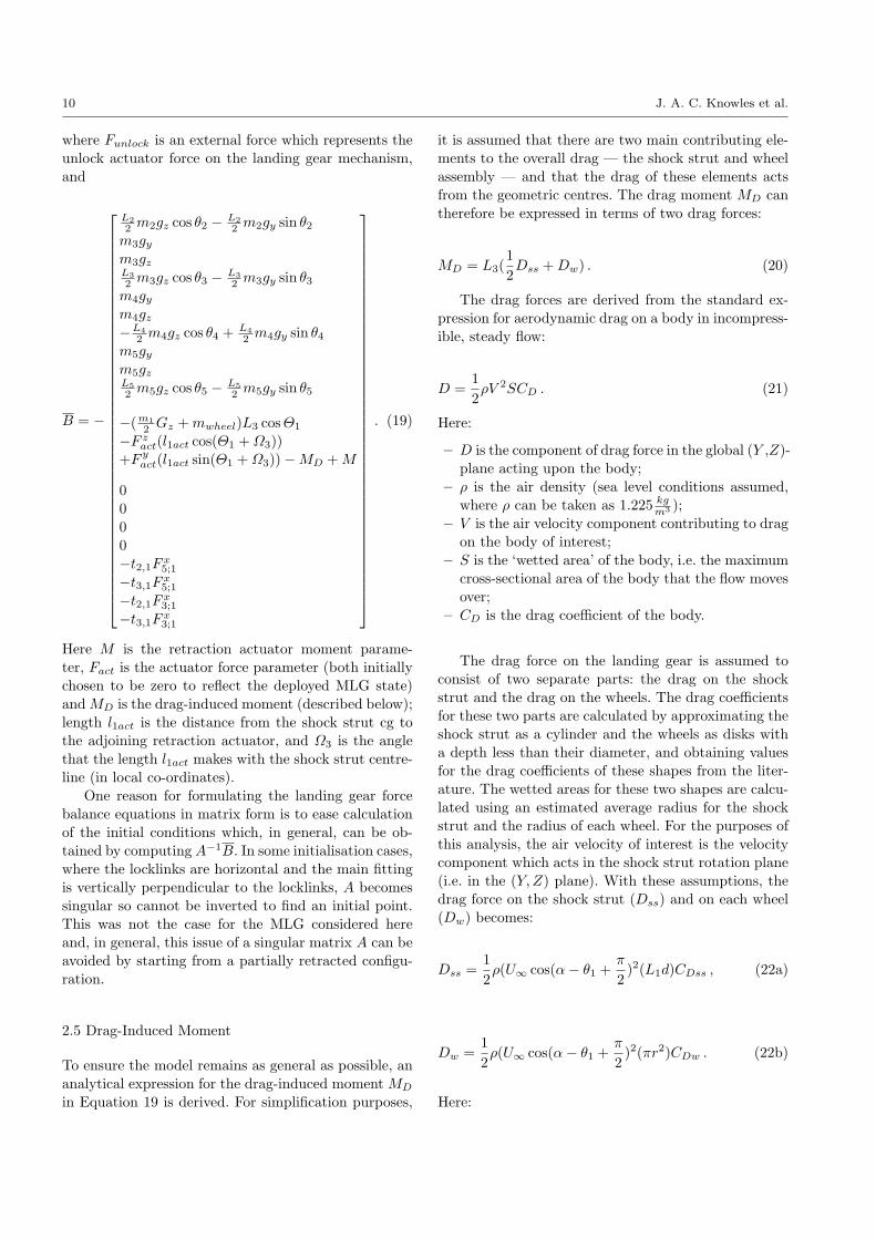
Here M is the retraction actuator moment parame-ter, Fact is the actuator force parameter (both initiallychosen to be zero to reflect the deployed MLG state)and MD is the drag-induced moment (described below);length l1act is the distance from the shock strut cg tothe adjoining retraction actuator, and Ω3 is the anglethat the length l1act makes with the shock strut centre-line (in local co-ordinates).

One reason for formulating the landing gear forcebalance equations in matrix form is to ease calculationof the initial conditions which, in general, can be ob-tained by computing A−1B. In some initialisation cases,where the locklinks are horizontal and the main fittingis vertically perpendicular to the locklinks, A becomessingular so cannot be inverted to find an initial point.This was not the case for the MLG considered hereand, in general, this issue of a singular matrix A can beavoided by starting from a partially retracted configu-ration.

2.5 Drag-Induced Moment

To ensure the model remains as general as possible, ananalytical expression for the drag-induced moment MD

in Equation 19 is derived. For simplification purposes,

it is assumed that there are two main contributing ele-ments to the overall drag — the shock strut and wheelassembly — and that the drag of these elements actsfrom the geometric centres. The drag moment MD cantherefore be expressed in terms of two drag forces:

MD = L3(12Dss +Dw) . (20)

The drag forces are derived from the standard ex-pression for aerodynamic drag on a body in incompress-ible, steady flow:

D =12ρV 2SCD . (21)

Here:

– D is the component of drag force in the global (Y ,Z)-plane acting upon the body;

– ρ is the air density (sea level conditions assumed,where ρ can be taken as 1.225 kg

m3 );– V is the air velocity component contributing to drag

on the body of interest;– S is the ‘wetted area’ of the body, i.e. the maximum

cross-sectional area of the body that the flow movesover;

– CD is the drag coefficient of the body.

The drag force on the landing gear is assumed toconsist of two separate parts: the drag on the shockstrut and the drag on the wheels. The drag coefficientsfor these two parts are calculated by approximating theshock strut as a cylinder and the wheels as disks witha depth less than their diameter, and obtaining valuesfor the drag coefficients of these shapes from the liter-ature. The wetted areas for these two shapes are calcu-lated using an estimated average radius for the shockstrut and the radius of each wheel. For the purposes ofthis analysis, the air velocity of interest is the velocitycomponent which acts in the shock strut rotation plane(i.e. in the (Y, Z) plane). With these assumptions, thedrag force on the shock strut (Dss) and on each wheel(Dw) becomes:

Dss =12ρ(U∞ cos(α− θ1 +

π

2)2(L1d)CDss , (22a)

Dw =12ρ(U∞ cos(α− θ1 +

π

2)2(πr2)CDw . (22b)

Here:

Numerical continuation analysis of a three-dimensional aircraft main landing gear mechanism 11

Table 1: Values of the parameters used in this case study.

Parameter Value Parameter Value Parameter Value

L1 2.90 m ω2 1.90 CDss 0.600L2 0.777 m Ω1 142 CDw 1.17L3 1.17 m Ω2 1.77 m1 2300 kgL4 0.419 m α 0 m2 200 kgL5 0.628 m U∞ 0 m/s m3 110 kg

l13 0.270 m ρ 1.225 kgm3 m4 7 kg

l15 1.12 m d 0.5 m m5 7 kgω1 136 r 0.4 m mwheel 400 kga 0.290 m b 0.290 m ψd 6

– U∞ is the magnitude of the air velocity in the (Y,Z)plane;

– α is the angle between the airflow direction and theglobal Y -axis (set to zero in this paper);

– d is the diameter of the main fitting;– CDss is the drag coefficient of the main fitting of the

landing gear– r is the radius of the landing gear wheel;– CDw is the drag coefficient of the wheel of the land-

ing gear

To calculate the resulting moment, the drag forceswere assumed to act at the c/g of their respective bod-ies, so:

MD = L3( 12Dss +Dw)

= 14ρ(U∞ cos(α− θ1 + π

2 )2

×(d(L23)CDss + 2πr2CDw) .

(23)

3 Bifurcation Analysis of Actuator Placement

This case study is presented to demonstrate the poten-tial benefits of using numerical continuation methods inthe design phase of an aircraft. The actuator positionhas a direct influence on several key design objectives,including the peak actuator force and the retractionefficiency. The results presented here are for a MLG re-tracting perpendicularly to the onset flow — as such,the air velocity, and hence the drag-induced momentMD in the model, is set to zero throughout. This cor-responds to the case of an aircraft flying in a straightline without experiencing any sideslip motion, which isa realistic case to consider for the purposes of this in-vestigation.

Table 1 provides details of the initial parameter val-ues used within the model during this case study. Thevalues were chosen to be representative of the MLG ofa generic medium-sized passenger aircraft’s main land-ing gear, such as a Boeing 737 or an Airbus A320. Itshould be noted though that these are only defined as

parameters by convention; the model flexibility enablesany of these parameters to be treated in the numericalcontinuation as a model state provided an appropriatenumber of other variables are fixed, however for the pur-pose of this case study these parameter values remainfixed.

3.1 Actuator Parameterisation

Figure 7 shows how the actuator position is parame-terised within the model. Three parameters are usedto describe the actuator position: length a denotes thevertical distance between the shock strut rotation pointand the actuator attachment point on the aircraft body;length b is the distance between the shock strut rotationpoint and the actuator attachment point on the shockstrut; and angle ψd is the angle made in the deployedposition between the actuator and the shock strut cen-treline. It should be noted that, whilst it would be pos-sible to parameterise the actuator position in terms ofthree length parameters (a, b and c = (a + b) tanψ)rather than two lengths and one angle, the three lengthparameters would not be independent, and thereforedistinguishing between parameter effects would be moredifficult.

The actuator is positioned in the plane that theshock strut retracts in, as any out of plane actuatorcomponents would not contribute to retracting the land-ing gear. The actuator is also assumed to be attachedto the shock strut centreline, something which is notnecessarily the case for all real landing gears. The pa-rameter a is fixed in the following results presented inthis paper, and chosen to be equal to 10% of the shock-strut length L1.

3.2 Influence of the Actuator Angle on Required Force

Figure 8(a) shows the curve of equilibrium solutionsthroughout the retraction cycle in terms of the actu-ator force F and retraction angle Θ1, for parameters

12 J. A. C. Knowles et al.

.

.

a

X

Z!d

b

Y

Z

(a + b) tan (!d)

n

Y

X

Fig. 7: Actuator parameterisation diagram.

.

.

045900

100

200

300

045900

100

200

300

(c)

F [kN]

!1 [deg] !d [deg]

(a)F [kN]

!1 [deg]

(b)F [kN]

!1 [deg]

Fig. 8: Retraction/extension equilibria for a = b =10%L1 shown in terms of actuator force F as a functionof retraction angle Θ1 for actuator angle ψd = 6 (a)and ψd = 50 (b). Panel (c) shows a surface of equilib-ria plotted in terms of F as a function of Θ1 and ψdbetween 6 and 50. The red curve denotes the localmaxima of F .

a = b = 0.29m, i.e. 10% of shock strut length L1, andan actuator moment angle of ψd = 6. The landing gearstarts in the deployed position with a retraction angleof Θ1 = 90. As the gear retracts, Θ1 decreases untilthe gear reaches the fully retracted position at Θ1 = 0.The plot in Figure 8(a) shows the equilibrium informa-tion in terms of the actuator force F that is required tohold the landing gear in static equilibrium at a givenretraction angle Θ1. To obtain smooth motion in a realretraction or extension of the landing gear, the forcevariation would need to approximate this equilibriumcurve.

The initially steep gradient is a result of the mecha-nism geometry; internal forces from the sidestay/locklinkplane are transmitted into the main fitting at the sidestayand locklink attachment points. The moments createdby these internal forces resist the initial motion of themain fitting, until the moment induced by the actu-ator overcomes the opposing moment of the sidestayand locklink forces. If the landing gear mechanism waslocked, the actuator moment required to overcome theinternal moments and begin the retraction cycle wouldbe very large (practically infinite). To enable the gear toretract, an unlock actuator is used to partially unlockthe locklinks before the retraction actuator retracts thegear.

Beyond the initial steep gradient, the actuator forcerequired to hold the landing gear in equilibrium con-tinues to increase as the landing gear retracts. This isbecause the out-of-plane gravitational forces acting onthe sidestays and locklinks increase more than the ac-tuator force projection working to retract the landing

Numerical continuation analysis of a three-dimensional aircraft main landing gear mechanism 13

gear. Beyond the local maximum force point, the land-ing gear requires less force from the actuator to hold thesystem in equilibrium as the retraction angle decreases:namely, beyond the local maximum, the out-of-planegravitational force increase during retraction is over-come by the increased actuator force projection actingto retract the landing gear.

The implication of this decreasing equilibrium forceis that the gear needs to be slowed down before itreaches the retracted position. For a constant landinggear actuator force value higher than the maximumequilibrium force, the landing gear will move upwardsinto the wing. In the absence of any actuator control,the landing gear will slam into the aircraft. To preventthis from happening, actuators used in service containa damping element that works to slow down the actu-ator retraction rate, in turn slowing the gear down sothat it comes to rest without impacting the wing box.

Figure 8(b) shows an equivalent curve of equilibriumsolutions for an actuator moment angle of ψd = 50.The curve is qualitatively different from the case ofψd = 6: the initial gradient is quite shallow and, asthe landing gear retracts, the gradient of this curveincreases. The reason for the relatively shallow initialgradient is that the retraction actuator has a muchlarger component acting to retract the landing gearwhen ψd = 50, so significantly less force is required tocreate the required retraction moment. Along the equi-librium curve, there is now no local maximum force;instead, the maximum actuator force for ψd = 50 isthe force required to hold the landing gear in the re-tracted state. The value of this maximum is slightlyhigher than the maximum force obtained for ψd = 6.

Figure 8(c) graphically represents how the retrac-tion equilibrium curve changes with different values ofψd between the two extreme cases shown in Figure 8(a)and (b). The surface of equilibria is bounded by a blackcurve for clarity, whilst the red curve on the surface isthe locus of local maxima. The local maxima curve in-dicates actuator configurations which have a maximumforce that occurs before the gear is fully retracted. Re-traction cycles with a local maximum force are quali-tatively similar to the case shown in Figure 8(a). Forvalues of ψd where no local maximum is present in theretraction cycle, the maximum force occurs at the endof the retraction cycle and the retraction response isqualitatively similar to the case shown in Figure 8(b).It can therefore be seen from Figure 8(c) that the lowestpeak actuator force is achieved for the actuator angleψd = 28, which is the value where the locus of localmaxima disappears.

3.3 Actuator Length Requirements

In a real MLG, physical constraints will limit the po-sitioning of the landing gear actuator. One of theseconstraints is the change in actuator length betweenthe deployed position (where the actuator is extended)and the retracted position (where the actuator is con-tracted).

Fig. 9: Dependence of actuator length Lact on retrac-tion angle Θ1 and actuator angle ψd for a moment armlength of b = 10%L1. Panels (a) and (b) show projec-tions onto the (Lact, Θ1)-plane and (Lact, ψd)-plane,respectively, of the surface in panel (c).

Figure 9 shows how the actuator length depends onthe retraction angle Θ1 and the actuator angle ψd whenthe gear is in equilibrium. The equilibrium surface inFigure 9(c) is simply a different projection of the sameequilibria shown in Figure 8(c); no new calculationswere needed. The (Lact, Θ1)-projection in Figure 9(b)shows that the maximum actuator length (which oc-curs in the deployed position) increases as the actua-tor angle is increased from 6 to 50. A result that isslightly less obvious is the change in minimum actua-tor length (which occurs in the retracted position). Thelower bound on the surface, shown in Figure 9(a), forms

14 J. A. C. Knowles et al.

a somewhat parabolic edge; the actuator length initiallydecreases as the actuator angle is increased before aminimum retracted actuator length occurs at ψd = 30.This minimum length occurs when the horizontal dis-tance between the actuator-airframe attachment pointand the shock strut attachment point ((a+ b) tanψd asin Figure 7) equals the actuator moment arm b. For thecase considered here where a = b = 10%L1, the min-imum actuator length occurs in the retracted positionwhen tanψd = 0.5, i.e. when ψd = 30.

3.4 Actuator Efficiency Dependency on ActuatorAngle

The efficiency E of the landing gear actuator is givenby the ratio of the area under the curve of actuatorforce F as a function of actuator length Lact (area B inFigure 10(a) and (b)) to the area of the rectangle whichbounds that curve (area A in Figure 10(a) and (b)) [3].The efficiencies for the two cases shown in Figures 10(a)and (b) are 92% and 43% respectively. As before, whenconsidering the retraction efficiency as the comparativemeasure, the case when ψd = 6 would be a betterchoice than using ψd = 50. The response shown inFigure 10(b) is of a type referred to by Conway [1] asa “bad retraction diagram”, compared to the “typicalretraction curve” of the response shown in Figure 10(a).

Figure 10(c) shows the equilibrium surface in (ψd,Lact, F )-space. As before, the edges of the surface arehighlighted by black curves and the red curve is the lo-cus of local maxima. The shadow on the bottom of thefigure shows the top-down projection of the surface (thesame view shown previously in Figure 9(a)). This fig-ure depicts graphically three conflicting design drivers:the peak actuator force, to be minimised; the changein actuator length, to be minimised; and the actuatorefficiency, to be maximised.

Figure 11 presents the three conflicting design driversobservable in Figure 10(c) in a more convenient man-ner. Figure 11(a) shows that the change in actuatorlength δLact increases approximately linearly with ψduntil about ψd = 30, when the gradient decreases untilthe maximum point on the graph is reached. As the de-sign driver would be to minimise δLact, a small actuatorangle would be most desirable from this perspective. Asmall value for ψd would also be desirable when consid-ering the efficiency variation in Figure 11(b). This plotshows that as the actuator angle increases, the efficiencydecreases. As a minimal δLact would generally be mostdesirable from a design perspective, there would be noconflict in meeting both efficiency and length changedesign objectives.

Fig. 10: Retraction/extension equilibria for a = b =10% shock strut length in terms of actuator force F ,actuator length Lact and actuator angle ψd, with ψdequal to (a) 6, (b) 50 and (c) between 6 and 50.The red curve in (c) denotes a fold bifurcation.

Figure 11(c) shows that the minimum peak actua-tor force Fact occurs above the lowest value of ψd con-sidered – far from the actuator angle that would min-imise δLact and maximise efficiency. It would thereforebe necessary to consider further factors (such as the in-fluence of these measures on actuator weight, operatingcost, manufacturing cost, etc.) to make an informed de-sign decision regarding actuator placement within thisexample landing gear system.

It should be noted that, whilst it would be possibleto use some form of optimising routine to attempt tofind an ‘optimum’ actuator position, the objective func-tion to be optimised heavily influences the outcome. Forpreliminary design work, the ability to accurately visu-alise how different parameters affect a variety of designobjectives allows a global picture of the underlying sys-tem behaviour to be built. Clear information about theimplications of design decisions, as provided here, mayaid the formulation of appropriate design criteria at anearly stage.

Numerical continuation analysis of a three-dimensional aircraft main landing gear mechanism 15

Fig. 11: Comparison of actuator length δLact (a); actuator efficiency E (b), and peak actuator force Fmax (c) withincreasing deployed actuator angle ψd.

3.5 Influence of Increasing Moment Arm

The effect of increasing the actuator moment arm b ispresented in Figure 12, where the corresponding changesto the surface of equilibria are shown. The case ex-amined up to this point is that in Figure 12(a) forb = 10%L1. Increasing the moment arm to b = 15%L1

reduces the peak actuator force required for a givenactuator angle. The overall effect is that the equilib-rium surface is now lower in the projections shown and,hence, for a given initial actuator angle, increasing b

would decrease the actuator force required to maintainthe gear in equilibrium at any given point throughoutthe retraction cycle. This is an intuitive result becausethe parameter b is the effective actuator moment arm.Further increases in b cause the peak actuator force tocontinue to decrease, although the amount of this forcereduction appears to diminish as b is increased throughFigures 12(c) to (f).

A less intuitive result is observed when consideringhow the locus of local maxima changes as b increases.From Figure 12(a) to (b), the curve of maxima movessuch that its endpoint at Θ1 = 0 disappears at a highervalue of ψd. This endpoint still coincides with the mini-mum peak actuator force point, so the equilibrium sur-face for b = 15%L1 is qualitatively similar to that forb = 10%L1. As b is increased further to b = 20%L1, aqualitative change in the surface is observed. The localmaxima curve moves such that its endpoint at Θ1 = 0no longer coincides with the minimum peak actuatorforce; see Figure 12(c). A further increase in the actua-tor moment arm from b = 20%L1 to b = 25%L1 causesthe disappearance of the local maxima curve from theψd range considered; see Figure 12(d) – (f).

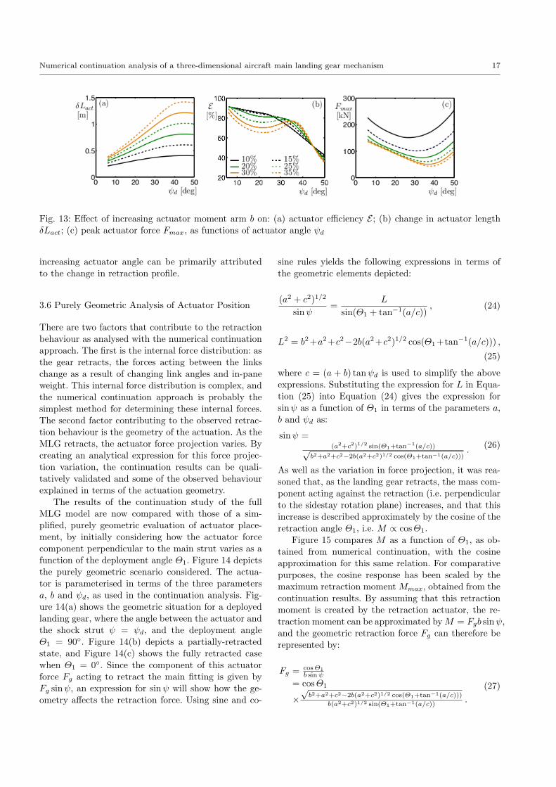
Figure 13 plots the efficiencies, change in actuatorlengths and peak forces for the six cases of actuatormoment arm b in Figure 12. As the change in actua-tor length is a purely geometric property of the sys-

tem, increasing b simply scales δLact. Hence, in Fig-ure 13(a), the shape of the curves remain unchangedqualitatively. This information enables physical boundsto be imposed on the actuator length change during theretraction cycle; since the actuator must fit in a con-fined space, the maximum actuator length is requiredto be kept within any space limits.

Figure 13(b) shows efficiency curves, which changesignificantly as b is increased. There is a qualitativechange that sees a second efficiency peak form for valuesof ψd ≈ 37% when b reaches 25%L1. The reason for thisqualitative change relates to several observable changesin the equilibrium surfaces of Figure 12 along with thevariation in maximum force depicted in Figure 13(c).These changes are explained by considering the two ex-treme cases for b (i.e. b = 10%L1 and b = 35%L1).

When b = 10%L1, the change in peak actuator forcewith actuator angle is relatively small, decreasing from230 kN to its minimum of 180kN as ψd increases from 6

to 27 Figure 13(c). Within this actuator angle range,the peak force occurs at the local maxima indicatedin Figure 12(a). In these cases, the load-displacementcurve has a sharp gradient initially which gradually de-creases to the maximum force value in a manner asshown in Figure 10(a), which is an efficient way toretract the gear. Once the local maxima have disap-peared, the peak force increases as ψd is increased, andthe retraction cycle begins to look more like the re-sponse shown in Figure 10(b), with a shallow gradientinitially that increases as the gear retracts. This typeof response is less efficient, as depicted by the efficiencycurve for b = 35% in Figure 13(b). It is interestingto note the abrupt change in gradient observed in the(ψd, E)-curve for b = 10%L1 when the actuator an-gle is increased beyond the angle of minimum actuatorforce (approximately ψd = 25). The change in gradientmeans that, whilst low actuator angles for b = 10%L1

provide an efficient retraction response, there is a range

16 J. A. C. Knowles et al.

.

.

(a)

F [kN]

!1 [deg] !d [deg]

(b)

F [kN]

!1 [deg] !d [deg]

(c)

F [kN]

!1 [deg] !d [deg]

(d)

F [kN]

!1 [deg] !d [deg]

(e)

F [kN]

!1 [deg] !d [deg]

(f)

F [kN]

!1 [deg] !d [deg]

Fig. 12: Surface of retraction/extension equilibria for different parameter values with b ranging from (a) 10% to(f) 35% of the shock strut length in steps of 5% for intermediate panels (b)-(e)

of actuator angles over which b = 10%L1 is actually theleast efficient of all the six actuator configurations in-vestigated. This shows just how sensitive the actuatorefficiency can be to changes in actuator placement, andhighlights the importance of design tools that can cap-ture counter-intuitive behaviour in a succinct manner.

When b has been increased to 35%, no local maximaare present on the equilibrium surface of Figure 12(f)and the percentage change in peak force over the actu-

ator angle range considered has increased significantly.Figure 13(c) shows that the maximum peak force whenb = 35%L1 is 140kN, and occurs when ψd = 6. As ψdincreases, this peak force value decreases linearly untilthe minimum peak force of 40kN is reached at ψd = 38.Over this range of retraction angles (i.e. 6 ≤ ψd ≤ 38)the relation between Lact and ψd shown in Figure 13(a)is also linear, so the resultant efficiency variation with

Numerical continuation analysis of a three-dimensional aircraft main landing gear mechanism 17

Fig. 13: Effect of increasing actuator moment arm b on: (a) actuator efficiency E ; (b) change in actuator lengthδLact; (c) peak actuator force Fmax, as functions of actuator angle ψd

increasing actuator angle can be primarily attributedto the change in retraction profile.

3.6 Purely Geometric Analysis of Actuator Position

There are two factors that contribute to the retractionbehaviour as analysed with the numerical continuationapproach. The first is the internal force distribution: asthe gear retracts, the forces acting between the linkschange as a result of changing link angles and in-paneweight. This internal force distribution is complex, andthe numerical continuation approach is probably thesimplest method for determining these internal forces.The second factor contributing to the observed retrac-tion behaviour is the geometry of the actuation. As theMLG retracts, the actuator force projection varies. Bycreating an analytical expression for this force projec-tion variation, the continuation results can be quali-tatively validated and some of the observed behaviourexplained in terms of the actuation geometry.

The results of the continuation study of the fullMLG model are now compared with those of a sim-plified, purely geometric evaluation of actuator place-ment, by initially considering how the actuator forcecomponent perpendicular to the main strut varies as afunction of the deployment angle Θ1. Figure 14 depictsthe purely geometric scenario considered. The actua-tor is parameterised in terms of the three parametersa, b and ψd, as used in the continuation analysis. Fig-ure 14(a) shows the geometric situation for a deployedlanding gear, where the angle between the actuator andthe shock strut ψ = ψd, and the deployment angleΘ1 = 90. Figure 14(b) depicts a partially-retractedstate, and Figure 14(c) shows the fully retracted casewhen Θ1 = 0. Since the component of this actuatorforce Fg acting to retract the main fitting is given byFg sinψ, an expression for sinψ will show how the ge-ometry affects the retraction force. Using sine and co-

sine rules yields the following expressions in terms ofthe geometric elements depicted:

(a2 + c2)1/2

sinψ=

L

sin(Θ1 + tan−1(a/c)), (24)

L2 = b2 +a2 +c2−2b(a2 +c2)1/2 cos(Θ1 +tan−1(a/c))) ,

(25)

where c = (a + b) tanψd is used to simplify the aboveexpressions. Substituting the expression for L in Equa-tion (25) into Equation (24) gives the expression forsinψ as a function of Θ1 in terms of the parameters a,b and ψd as:

sinψ =(a2+c2)1/2 sin(Θ1+tan−1(a/c))√

b2+a2+c2−2b(a2+c2)1/2 cos(Θ1+tan−1(a/c))).

(26)

As well as the variation in force projection, it was rea-soned that, as the landing gear retracts, the mass com-ponent acting against the retraction (i.e. perpendicularto the sidestay rotation plane) increases, and that thisincrease is described approximately by the cosine of theretraction angle Θ1, i.e. M ∝ cosΘ1.

Figure 15 compares M as a function of Θ1, as ob-tained from numerical continuation, with the cosineapproximation for this same relation. For comparativepurposes, the cosine response has been scaled by themaximum retraction moment Mmax, obtained from thecontinuation results. By assuming that this retractionmoment is created by the retraction actuator, the re-traction moment can be approximated byM = Fgb sinψ,and the geometric retraction force Fg can therefore berepresented by:

Fg = cosΘ1b sinψ

= cosΘ1

×√b2+a2+c2−2b(a2+c2)1/2 cos(Θ1+tan−1(a/c)))

b(a2+c2)1/2 sin(Θ1+tan−1(a/c)).

(27)

18 J. A. C. Knowles et al.

Fig. 14: Geometry of landing gear actuator (thick line of variable length L) and shock strut (thin solid line of fixedlength b) shown in the deployed position (ψ = ψd) in (a), a partially-retracted state in (b), and the fully retractedposition in (c).

.

.0 45 900

1

2

3

4

5x 104

!1 [deg]

M[Nm]

Fig. 15: A comparison of the retraction moment M

as a function of retraction angle Θ1 as obtainedfrom the continuation analysis (solid grey curve) withMmax cosΘ1 (dashed black curve).

This expression comprises the purely geometric ef-fect of the changing actuator force projection sinψ givenby Equation (26), along with a significantly simplifiedrepresentation of the effect of the landing gear mass. Inparticular, Equation (27) does to include the (geomet-rically unknown) mass, meaning that Fg is effectivelynon-dimensionalised. Furthermore, the analytical for-mula still requires numerical analysis tools to evaluateand interpret the equation.

Figure 16 plots Fg from Equation (27) as a functionof Θ1 in panels (a) and (b). It should be noted thatno units have been assigned to the actuator force vari-able Fg since it is in units of landing gear weight. Withthe inclusion of the moment variation, it can be seen

that Equation (27) captures the variation in equilibriumsolutions shown in the continuation results. Further-more, the surface produced from the geometric analysisin Figure 16(c) also reflects how the loci of equillibriachange as the actuator moment arm b is varied. Thissuggests that the relatively simple Equation (27) cap-tures much of the essence of the behaviour seen in thecontinuation analysis results. In this case, it providesa qualitative validation of the continuation results thathighlights the effects of actuator geometry on the re-traction cycle properties.

There are, however, some differences between thegeometric force Fg and the equivalent numerical con-tinuation analysis result for the retraction force F fromFigure 8. For Fg, the shape of the response obtainedfor low ψd values is flatter2, whilst for high values ofψd the geometric analysis produces a response with amore pronounced force peak at the end of the retractioncycle. The reasons for these differences are attributedto the way the geometric analysis accounts for the restof the landing gear structure. The assumption that theweight moment opposing the retraction motion varies ina cosine manner is approximately true but not exact.Figure 15, where the moment required to retract theMLG (in grey) is plotted alongside Mmax cosΘ1, showsthat the actual moment variation is not exactly a co-sine; in particular, the peak occurs beyond the fully re-tracted position (i.e. Θ1 < 0). Moreover, other aspectsof the force balance in the MLG are also not modelledgeometrically.

2 i.e. the gradient either side of the local maximum pointremains quite shallow for a wide range of retraction anglevalues

Numerical continuation analysis of a three-dimensional aircraft main landing gear mechanism 19

.

.

045900

10

20

30

045900

10

20

30

(c)

Fg

!1 [deg] !d [deg]

(a)Fg

!1 [deg]

(b)Fg

!1 [deg]

Fig. 16: Variation of theoretical actuator force F duringthe retraction cycle for the case when a = b = 10%L1

with deployed actuator angles of ψd = 1 in (a), ψd =60 in (b), and between 1 and 60 in (c).

4 Concluding Remarks

It has been shown how a three-dimensional main land-ing gear retraction mechanism can be modelled as aset of fully parameterised steady-state constraint equa-tions. This modelling approach is relatively simple yetflexible, and ideally suited for the use of numerical meth-ods from bifurcation theory. In particular, it enablesdifferent landing gear configurations to be investigatedwith relative ease, saving modelling time by avoidingthe need to make major model adaptations for a newgear configuration. The numerical continuation approachtakes full advantage of this flexible formulation, allow-ing any model parameter of interest to be varied con-tinuously. This is an advantage over traditional multi-body dynamic simulations that are confined to runningindividual simulations for fixed values of system param-eters.

The modelling and analysis approach was demon-strated with an investigation of MLG actuator place-ment from a design perspective. Several design param-eters associated with the landing gear actuator were

changed to investigate the resulting change in the re-traction cycle. The numerical continuation approach al-lowed for convenient representation of equilibrium sur-faces as functions of two design parameters: the modelformulation complemented this by providing values forall states within the MLG mechanism directly, with-out needing to post-process the data to determine geo-metric dependencies of one model state of interest as afunction of another. Increasing the actuator angle wasshown to initially reduce the peak actuator force re-quirement, but there is a trade-off as the efficiency ofthe retraction cycle decreases over this same range. Aswell as providing information regarding retraction effi-ciency and peak actuator force, the model provided ac-tuator length details from the same continuation data.It was suggested that this could be used to providebounds to the design space when positioning the ac-tuator based on space constraints within the airframe.

The numerical continuation approach was comparedto a purely geometric model of actuator force projec-tion. This highly simplified model qualitatively sup-ported the findings from the numerical continuationanalysis, and was useful for providing some insight intothe underlying generic mechanisms. The purely geomet-ric model however, does not consider the internal forcebalance and was found to be unable to provide qual-itatively reliable results, thus strengthening the casefor performing a continuation analysis of the full MLGequations.

With the increasing use of composite materials inprimary structural elements of the next generation civilaircraft, future landing gear designs may require novelways of reducing the point loads transferred into a car-bon fibre wing box structure. One method of achiev-ing this is to use a dual sidestay landing gear to re-distribute the loads over multiple attachment points onthe aircraft. The modelling approach presented here canbe extended to a dual sidestay landing gear, resultingin 36 geometric constraints and 36 internal force con-straints. The flexible approach offered by formulatingthe dual sidestay mechanism as a set of steady-stateconstraint equations, would enable design parameters,such as the angle between the two sidestays or the massof a link, to be used as a continuation parameter in aninvestigation of the retraction cycle — something noteasily achievable with conventional dynamic simulationmethods.

References

1. Conway, H.G., Landing Gear Design, pp 1–4. Chapmanand Hall, London, 1958.

2. Knowles, J.A.C., Krauskopf, B., Lowenberg, M.H., Nu-merical Continuation Applied to Landing Gear Mechanism

20 J. A. C. Knowles et al.

Analysis, AIAA Journal of Aircraft, Vol. 49, No. 8, July –August 2011.

3. Currey, N.S., Aircraft Landing Gear Design: Principlesand Practices, pp 152–172. AIAA, Washington D.C, 1988.

4. Strogatz, S., Nonlinear dynamics and chaos, Springer,2000.

5. Guckenheimer, J. and Holmes, P., Nonlinear Oscillations,Dynamical Systems and Bifurcations of Vector Fields,Applied Mathematical Sciences Vol. 42, Westview Press,February 2002.

6. Krauskopf, B., Osinga, H. M., and Galan-Vioque, J.,Numerical Continuation Methods for Dynamical Systems,Springer, 2007.

7. Rankin, J., Coetzee, E., Krauskopf, B. and Lowenberg,M., Bifurcation and Stability Analysis of Aircraft Turningon the Ground, AIAA Journal of Guidance, Dynamics andControl, Vol. 32, No. 2, March 2009.

8. Coetzee, E., Krauskopf, B. and Lowenberg, M,. Applica-tion of Bifurcation Methods to the Prediction of Low-SpeedAircraft Ground Performance AIAA Journal of Aircraft,Vol. 47, No. 4, July – August 2010

9. Thota, P., Krauskopf, B. and Lowenberg, M., Interactionof Torsion and Lateral Bending in Aircraft Nose LandingGear Shimmy, Nonlinear Dynamics, 57(3), 2009.

10. Doedel, E., Champneys, A., Fairgrieve, T., Kuznetsov,Y., Sandstede, B., and Wang, X., AUTO 97 : Continuationand bifurcation software for ordinary differential equations,http://indy.cs.concordia.ca/auto/, May 2001.

11. Coetzee, E.B., Krauskopf, B., Lowenberg, B.,”Dynamical Systems Toolbox for MATLAB,”https://github.com/ecoetzee/Dynamical-Systems-Toolbox, July 2011

12. Hoerner, S. F., Aerodynamic Drag, pp 27–30. Ohio, 1951