An-Najah National University Faculty of Graduate Studies Numerical Simulation of Seawater Intrusion in Response to Climate Change Impacts in North Gaza Coastal Aquifer Using SEAWAT By Reem Fathi Saleh Sarsak Supervisor Dr. Mohammad N. Almasri Submitted in Partial Fulfillment of the Requirements for the Degree of Master of Water and Environmental Engineering, Faculty of Graduate Studies, at An-Najah National University, Nablus, Palestine 2011
Transcript
An-Najah National University Faculty of Graduate Studies
Numerical Simulation of Seawater Intrusion in Response to Climate Change Impacts in North
Gaza Coastal Aquifer Using SEAWAT
By Reem Fathi Saleh Sarsak
Supervisor Dr. Mohammad N. Almasri
Submitted in Partial Fulfillment of the Requirements for the Degree of Master of Water and Environmental Engineering, Faculty of Graduate Studies, at An-Najah National University, Nablus, Palestine
2011
iii
Dedication
I proudly dedicate this thesis to the soul of my father, to my beloved
mother, as I always feel her prayers in all aspects of my life, and finally my
husband Bashar for his great encouragement and support, and my three
lovely children Ahmad, Mohammad and Abdullah.
iv
ACKNOWLEDGEMENTS
Great appreciation and thanks to Dr. Mohammad N. Almasri, who served
as the chairman on my thesis committee, is nothing compared to what I
actually feel for his unparalleled supervision, help and guidance. He has
been the constant source of encouragement, inspiration, help and patience. I
would like to express my gratitude to Dr. Amjad Aliewi for his interest in
this work and time and helpful suggestions in addition to the advice given
by him. I am grateful to Dr. Anan Jayousi for serving on my thesis
committee. I would sincerely like to thank Dr. Said Ghabayen and Dr.
Khalid Qahman for their cooperation as this work would not have been
accomplished without their kind help. I would like to express my
appreciation to PWA team in Ramallah for their cooperation and help to
get data with special thanks to Eng. Ahmad Al-Yaqubi whose suggestions
were helpful.
Reem F. Sarsak
Nablus, 2011
v
قـراراإل
:الرسالة التي تحمل العنوان ةأدناه مقدم ةا الموقعأن
Numerical Simulation of Seawater Intrusion in Response to Climate Change Impacts in North Gaza
Coastal Aquifer Using SEAWAT
دراسة تأثير التغيرات المناخية على دخول المياه المالحة الى الحوض الجوفي
SEAWATباستخدام شمال غزةالساحلي في
أقر بأن ما اشتملت عليه هذه الرسالة إنما هي نتاج جهدي الخاص، باستثناء مـا تمـت
اإلشارة إليه حيثما ورد، وأن هذه الرسالة ككل، أو أي جزء منها لم يقدم من قبل لنيل أية درجة
.علمية أو بحث علمي أو بحثي لدى أية مؤسسة تعليمية أو بحثية أخرى
Declaration
The work provided in this thesis, unless otherwise referenced, is the
researcher's own work, and has not been submitted elsewhere for any other
degree or qualification.
:Student's name :ةاسم الطالب
:Signature : التوقيع
:Date : التاريخ
vi
TABLE OF CONTENTS No. Contents Page
Acknowledgments iv Declaration v Table of Contents vi List of Tables vii List of Figures ix List of Appendices xi Abbreviations Table xii Abstract xiii Chapter 1: INTRODUCTION 1 1.1 General Background 2 1.2 Objectives 4 1.3 Research questions 41.4 Methodology 5 1.5 Thesis outline 7
Chapter 2: DESCRIPTION OF THE STUDY AREA
8
2.1 Geographic Location 9 2.2 Study Area Outline 102.3 Population 11 2.4 Geology 12 2.5 Land use 132.6 Climate 14 2.7 Existing water problems in Gaza Strip 15 2.8 Water Balance 17 2.9 Well Status in the Study Area 18 2.10 A Brief Overview of Water Quality in the Study Area 18 2.11 Demand components 20 2.12 Future Municipal Water Needs 21 Chapter 3: LITERATURE REVIEW 22 3.1 Introduction 23 3.2 SEAWAT Applications 23
Chapter 4: CLIMATE CHANGE - A GENERAL BACKGROUND
28
4.1 Definition of Climate Change 29 4.2 Impacts of Climate Change 29 4.3 Predictions of Climate Change for the Middle East 29 4.4 Predictions of Climate Change for the Mediterranean 31
vii
No. Contents Page 4.5 Climate Change Scenarios 34 4.5.1 Temperature 35 4.5.2 Precipitation 35 4.5.3 Sea Level Rise 36 Chapter 5: SEAWATER INTRUSION 38 5.1 General Background and Definition 39 5.2 Consequences and Assessments 405.3 How to assess Seawater Intrusion? 40 5.4 SEAWAT Concept 42 5.4.1 SEAWAT Procedure 44 5.4.2 Governing Equations 45
Chapter 6: DEVELOPMENT OF THE SEAWAT MODEL FOR THE NORTH GAZA AREA
48
6.1 Introduction 49 6.2 Basic Groundwater Flow Model 49 6.2.1 Recharge Components 51 6.2.2 Abstraction Wells 52 6.2.3 Simulation Period 53 6.2.4 Steady State Model Calibration 53 6.3 SEAWAT Model Development 54 6.3.1 Simulation Period for SEAWAT Model 55 6.3.2 Boundary Conditions 56 6.3.3 Calibration of the SEAWAT Model 57 6.4 The Studied Scenarios 59 6.5 Results of Scenarios Simulation 62 6.5.1 Scenario 1: Existing conditions 62 6.5.2 Scenario 2: Sensitivity to pumping rates 67 6.5.3 Scenario 3: Impacts of sea level rise 72 6.5.4 Scenario 4: Sensitivity to recharge 75 6.5.5 Scenario 5: Extreme impacts of climate change 79 6.5.6 Scenario 6: Management scenario 82 6.5.7 Overall Discussion 85
Table (1) Population Growth Rates 11 Table (2) Population Projections in the Study Area 12
Table (3) Agriculture production areas (Hectares) in North Gaza 14
Table (4) Water Balance for Hydrological year 2008/2009 of the Gaza Strip 17
Table (5) Water Balance for Hydrological year 2008/2009 of the Study Area 17
Table (6) Summary of the Total Water Demand for all sectors for 2009 in the Study Area 21
Table (7) Climate Change projections for Gaza Strip 34
Table (8) Average Seasonal Abstraction rates from Municipal wells 53
Table (9) Input parameters for the SEAWAT model 57
Table (10) Summary description of the different scenarios simulated by the SEAWAT model 60
Table (11) Summary of scenarios results by the end of simulation period (year 2035) 85
ix
LIST OF FIGURES No. Figure Page
Figure (1) Warming world indicators 2 Figure (2) A Flowchart of research methodology 6 Figure (3) Regional Setting of Gaza Strip 9 Figure (4) Study Area Outline 10
Figure (5) NW-SE Hydro-geological cross section of Gaza Strip 13
Figure (6) Land use distribution of the Study Area 14
Figure (7) The average annual rainfalls of the Study Area (1980-2010)strip (1980-2010) 15
Figure (8) Steady State Water Level Contour Map for the Study Area 16
Figure (9) Wastewater problems at Gaza Strip 17
Figure (10) Chloride Concentration of Domestic Municipal Wells for year 2009 19
Figure (11) Nitrate Concentration of Domestic Municipal Wells for year 2009 20
Figure (12) Regional Climate Model projections of average temperature changes (ºC) across the Gulf region 31
Figure (13) Regional Climate Model projections of precipitation changes (%) across the Gulf region 31
Figure (14) The winter (DJF) predicted change in the mean seasonal precipitation (mm) 33
Figure (15)
The summer (JJA- June, July, and August) predicted change in the daily mean maximum temperature. Differences are between A2 and B2 scenarios
34
Figure (16) Melting of glaciers and ice caps 36
Figure (17) (a): Clarifications of Ghyben-Herzberg theory, (b): effect of pumping into freshwater/seawater interface
39
Figure (18) Time series of global mean sea levels 41
Figure (19) Two piezometers, one filled with freshwater and the other with saline aquifer water, open to the same point in the aquifer
44
Figure (20) Model Boundaries and Grid 50
Figure (21) Bottom of the aquifer and the ground surface elevation 51
Figure (22) Head observation wells and MODFLOW recharge zones 52
x
No. Figure Page Figure (23) Steady state calibration results 54
Figure (24) A Flowchart for SEAWAT development selected wells for year 2009 55
Figure (25) Observed versus Simulated concentration for selected wells for year 2009 58
Figure (26) Locations of domestic wells from the sea shoreline wells 62
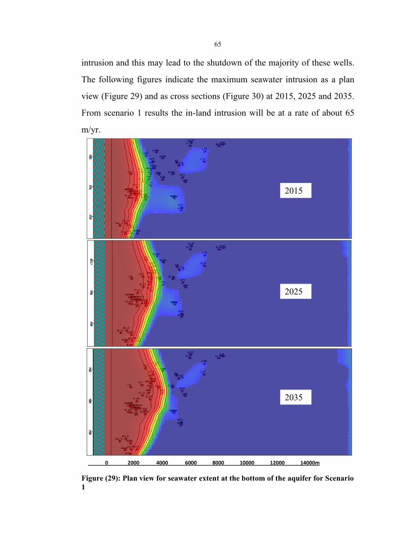
Figure (27) Simulated Chloride concentration at the selected wells for Scenario 1 63
Figure (28) In-Land Seawater Intrusion for Scenario 1 64
Figure (29) Plan for Seawater Interface at the bottom of the aquifer for Scenario 1 65
Figure (30) Cross section for Scenario 1 indicates the Maximum Seawater Interface at Row 35 66
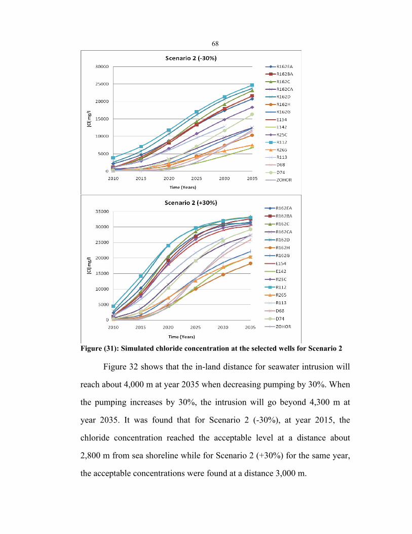
Figure (31) Simulated Chloride concentration at the selected wells for Scenario 2 68
Figure (32) In-Land Seawater Intrusion for Scenario 2 69
Figure (33) Cross section for Scenario 2 indicates the Maximum Seawater Interface at Row 35 71
Figure (34) Simulated Chloride concentration at the selected wells for Scenario 3 72
Figure (35) In-Land Seawater Intrusion for Scenario 3 73
Figure (36) Cross section for Scenario 3 indicates the Maximum Seawater Interface at Row 35 74
Figure (37) Simulated Chloride concentration at the selected wells for Scenario 4 75
Figure (38) In-Land Seawater Intrusion for Scenario 4 76
Figure (39) Cross section for Scenario 4 indicates the Maximum Seawater Interface at Row 35 78
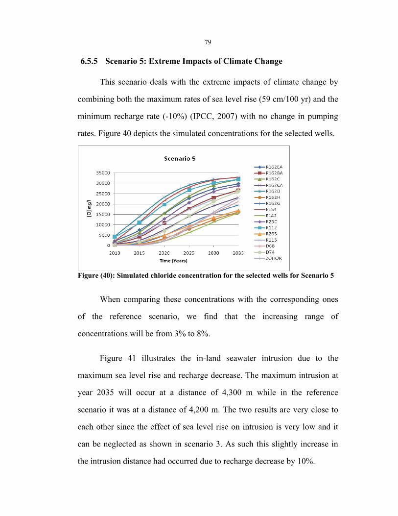
Figure (40) Simulated Chloride concentration at the selected wells for Scenario 5 79
Figure (41) In-Land Seawater Intrusion for Scenario 5 80
Figure (42) Cross section for Scenario 5 indicates the Maximum Seawater Interface at Row 35 81
Figure (43) Simulated Chloride concentration at the selected wells for Scenario 6 82
Figure (44) In-Land Seawater Intrusion for Scenario 6 83
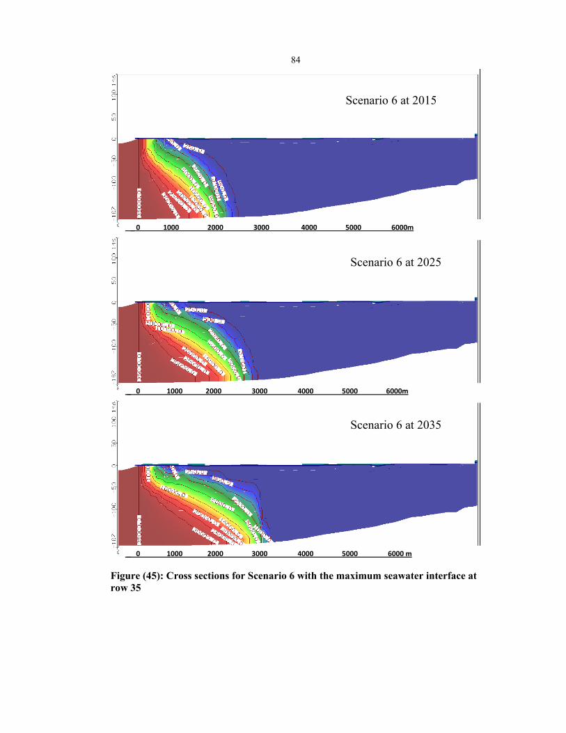
Figure (45) Cross section for Scenario 6 indicates the Maximum Seawater Interface at Row 35 84
Figure (46) Seawater Intrusion results for various Scenarios 85
xi
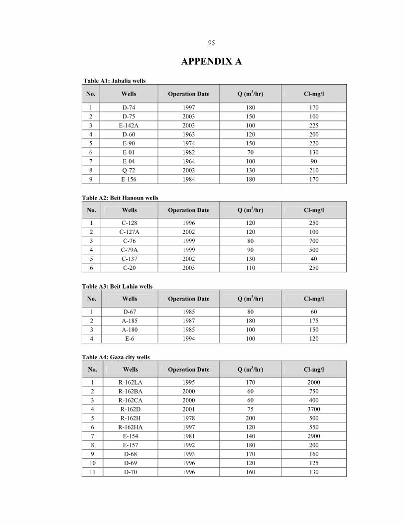
LIST OF APPENDICES No. Appendices Page Table A1 Jabalia Water Wells 95 Table A2 Beit Hanoun Water Wells 95 Table A3 Beit Lahia Water Wells 95 Table A4 Gaza Governorate Water Wells 95
Table A5 Target Consumption and Needs Rates at the Study Area 96
Table A6 The Spearman Rank Correlation between Observation Vs. simulation chloride concentration
96
Table A7 Average Quantity of Treated Wastewater 97 Table A8 Existing Desalination Plants production 99Table A9 Centralized Desalination plant 99 Table A10 Proposed Desalination Plants production 99
xii
ABBREVIATIONS [Cl] Chloride Concentration DJF December, January and February EM Eastern Mediterranean EMCC Engineering and Management Consulting Center GIS Geographical Information System JJA June, July, and Augustl/c/d Liter Per Capita Per Day m3 Cubic Meter m3/h Cubic Meter Per Hour m3/year Cubic Meter Per Year MCM Million Cubic Meter MCM/yr Million Cubic Meter per Year mg/l Mille Gram per Liter MoA Ministry of AgricultureMOPIC Ministry of Planning and International Cooperation NOAA National Oceanic and Atmospheric Administration PCBS Palestinian Central Bureau of Statistics PWA Palestinian Water Authority RCM Regional Climate Modeling
SEAWAT A Computer Program For Simulation of Three-Dimensional Variable-Density Groundwater Flow
WHO World Health Organization WWTP Wastewater Treatment Plant
xiii
NUMERICAL SIMULATION OF SEAWATER INTRUSION IN RESPONSE TO CLIMATE CHANGE IMPACTS IN NORTH GAZA
COASTAL AQUIFER USING SEAWAT By
Reem Fathi Sarsak Academic Advisor
Dr. Mohammad N. Almasri
ABSTRACT
The development and management of fresh groundwater resources in
coastal aquifers are seriously constrained by the presence of seawater
intrusion. Seawater intrusion is a process that occurs in almost all coastal
aquifers, where they are in hydraulic connection with seawater. Over the
years, many models have been developed to simulate and study the
problems related to seawater intrusion. Numerical models provide effective
tool to understand groundwater problems. This research presents simulation
of seawater intrusion in North Gaza coastal aquifer in response to climate
change impacts using SEAWAT. Climate change is already beginning to
transform life on earth. Around the globe, seasons are shifting, rainfalls are
decreasing, temperatures are climbing so water demands are increasing and
sea levels are raising causing seawater intrusion. If we don't act now,
climate change will permanently alter the lands and waters we all depend
upon for survival.
Various scenarios were simulated to study the impacts of climate
change into seawater intrusion at the study area due to sea level rise,
recharge and pumping rates variability.
xiv
The results show that the in-land movement for seawater intrusion
for the reference scenario (Scenario 1) which reflects the continuation of
the current situation is about 4,200 m with a rate of 65 m/yr. The most
critical extent of salinity was found in Scenario 4 (Recharge -30%) which
causes in-land intrusion movement of about 4,500m with a rate of 80 m/yr.
While the in-land intrusion movement due to increasing pumping rates as
in Scenario 2 (pumping +30%) was about 4,300 m with a rate of 70 m/yr.
The best results for the in-land intrusion were found in Scenario 6 which
considered as a management scenario since it is dealing with the proposed
strategic plans that were prepared by PWA to solve the high salinity
problems and water deficit in Gaza aquifer, the in-land intrusion movement
for this scenario was about 2,900m with a rate of 35 m/yr.
As a result, seawater intrusion in the study area is very sensitive to
recharge decrease as compared to pumping rates increase. As such, the
most critical impact on seawater intrusion for the study area is recharge
variability due to climate change. Therefore, it is recommended to search
for new resources such as desalination of seawater and brackish water in
addition to reuse of treated wastewater in order to reduce the gap in both
domestic and agricultural sectors respectively in case of recharge decrease
due to climate change.
1
CHAPTER ONE
INTRODUCTION
2
1.1 General Background
Global warming and climate change have been an active research
topic in the last decade. Natural events and human activities are believed to
be contributing to an increase in average global temperatures. This is
caused primarily by increases in “greenhouse” gases such as Carbon
Dioxide (CO2) (Global Issues, 2010).
As explained by the National Oceanic and Atmospheric
Administration (NOAA) in the US agency, there are seven indicators (see
Figure 1) that would be expected to increase in a warming world, and three
indicators would be expected to decrease. Water expands when heated, and
sea levels are expected to rise due to climate change. Rising sea levels will
also result as the polar caps begin to melt (Global Issues, 2010).
Figure (1): Warming world indicators (Source: NOAA, July 2010)
3
Global climate change is interrupting the water circulation balance
by changing rates of precipitation, recharge, discharge, and
evapotranspiration. The Intergovernmental Panel on Climate Change
(IPCC, 2007) makes “changes in rainfall pattern due to climate changes
and consequent shortage of available water resource” a high priority as the
weakest part among the effects of human environment caused by future
climate changes. Groundwater, which occupies a considerable portion of
the world’s freshwater resources, is related to climate change via surface
water such as rivers, lakes, and marshes, and direct interactions, being
indirectly affected through recharge (Lee, 2009).
Climate change is already beginning to transform life on
earth. Around the globe, seasons are shifting, rainfalls are decreasing,
temperatures are climbing so water demands are increasing and sea levels
are raising causing seawater intrusion. If we don't act now, climate change
will permanently alter the lands and waters we all depend upon for survival
(IPCC, 2007).
Seawater intrusion is a common contamination problem in coastal
areas. It affects, mainly, arid and semi-arid zones, where dense population
and urban development are coupled to scarce water resources and require
intense exploitation of groundwater. The Mediterranean coast is a good
example (Elina, 2006).
Gaza coastal aquifer met with the above problems such as dense
population semi- arid and water scarcity, for that it is a good example for
4
seawater intrusion problem due to over pumping and climate change
impacts such as recharge decrease and sea level rise.
1.2 Objectives
The main objective of this research is to assess the impacts of
climate change into seawater intrusion in North Gaza coastal aquifer using
SEAWAT.
The specific objectives in this research are to study the following:
The impact of pumping rate variability.
The impact of maximum sea level rise.
The impact of recharge variability.
The extreme impact of climate change due to maximum sea level rise
in addition to recharge variability.
Management solutions for water scarcity by using additional water
resources.
1.3 Research Questions
The following are the research questions:
1. What is the impact of climate change on seawater intrusion in North
Gaza coastal aquifer?
2. What are the potential management scenarios that can be considered
for the control of seawater intrusion in North Gaza coastal aquifer?
5
1.4 Methodology
Figure (2) depicts the methodology that was followed in this
research. The methodology starts by the collection of needed data from all
available sources such as documents, reports, maps and the communication
with local specialized persons from Gaza.
Data needed includes aquifer parameters such as hydraulic
conductivity, total and effective porosity, specific storage, etc…, changes
in rainfall patterns, and pumping rates. The population forecast was
determined to estimate the water demand and the expected quantity of
treated wastewater to be used in the agricultural sector at the end of the
study period in order to reduce the amount of pumping water for
agricultural sector. In order to reduce the amount of pumping water for
domestic sector, calculations were done for desalination water quantities
for both of brackish and sea water desalination plants.
The key data was obtained from MoA regarding to rainfall patterns
at the study area, and from PWA which is the hydrologic data for pumping
wells, this includes pumping rates and chloride concentrations for the years
2000 and 2009 for North Gaza wells, in addition to the basic needs and
development ongoing and proposed projects in the PWA strategic plans
such as desalination plants and wastewater treatment plants at Gaza Strip.
After preparation and processing, the data was analyzed using
EXCEL. The SEAWAT code (a three dimensional model of coupled
6
density-dependent flow and miscible salt transport), was selected to
simulate solute transport in order to predict and assess the impacts of
climate change on Gaza aquifer.
Six scenarios were formulated and assessed using SEAWAT to study
the three climate change impacts mentioned earlier in the objectives.
The results obtained from the model runs were analyzed. Based on
the research outcomes, the conclusions and recommendations were made.
Data Collection
Literature Review
Data Preparation and Processing
Data Analysis
Conclusions and Recommendations
Development of the Climate Change Scenarios
Analysis of Results
¤ Documents and Reports¤ Maps¤ Personal Communications
Development of the Numerical Model (SEAWAT)
Utilization of the Basic Groundwater Flow Model and
Solute Transport Model
Figure (2): A Flowchart of research methodology
7
1.5 Thesis Outline
The thesis is organized in seven chapters as follows. Chapter 1 gives
an introduction along with background information, objectives, research
questions and the methodology. Chapter 2 describes the study area. Chapter
3 provides the literature review. Chapter 4 gives a general definition of
climate change and its related scenarios. Chapter 5 illustrates the concept of
seawater intrusion. Chapter 6 highlights the different outcomes of the
climate change scenarios using SEAWAT model along with analysis.
Conclusions and recommendations are furnished in Chapter 7.
8
CHAPTER TWO
DESCRIPTION OF THE STUDY AREA
9
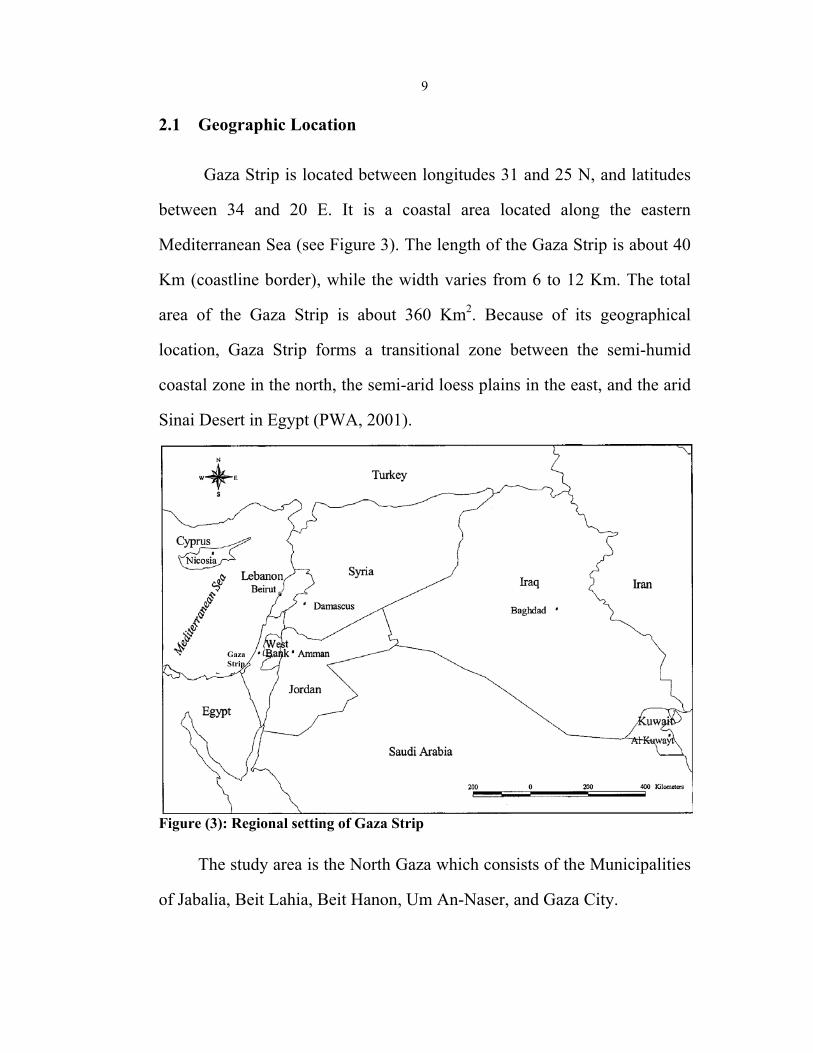
2.1 Geographic Location
Gaza Strip is located between longitudes 31 and 25 N, and latitudes
between 34 and 20 E. It is a coastal area located along the eastern
Mediterranean Sea (see Figure 3). The length of the Gaza Strip is about 40
Km (coastline border), while the width varies from 6 to 12 Km. The total
area of the Gaza Strip is about 360 Km2. Because of its geographical
location, Gaza Strip forms a transitional zone between the semi-humid
coastal zone in the north, the semi-arid loess plains in the east, and the arid
Sinai Desert in Egypt (PWA, 2001).
Figure (3): Regional setting of Gaza Strip
The study area is the North Gaza which consists of the Municipalities
of Jabalia, Beit Lahia, Beit Hanon, Um An-Naser, and Gaza City.
Gaza Strip
10
2.2 Study Area Outline
Figure (4) indicates the study area and coastal aquifer boundary.
Figure (4): Study area outline
The study area was extended to include additional area outside the
North Gaza borders to minimize the effects of model boundaries in the
central part of the model which is the main objective for this research.
The study area was determined based on the MODFLOW model
which was prepared in 2006 by PWA and EMCC (Engineering and
Management Consulting Center) to study the Environmental Assessment
for North Gaza Emergency Sewage Treatment Plant Project. This model
Study Area Boundary
The Coastal Aquifer Boundaries
11
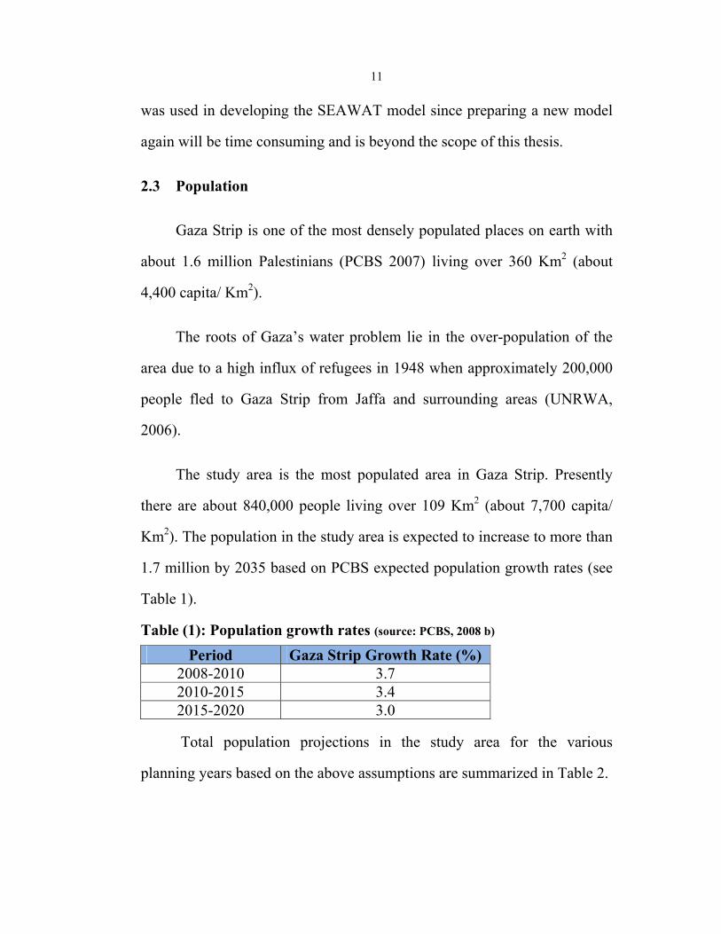
was used in developing the SEAWAT model since preparing a new model
again will be time consuming and is beyond the scope of this thesis.
2.3 Population
Gaza Strip is one of the most densely populated places on earth with
about 1.6 million Palestinians (PCBS 2007) living over 360 Km2 (about
4,400 capita/ Km2).
The roots of Gaza’s water problem lie in the over-population of the
area due to a high influx of refugees in 1948 when approximately 200,000
people fled to Gaza Strip from Jaffa and surrounding areas (UNRWA,
2006).
The study area is the most populated area in Gaza Strip. Presently
there are about 840,000 people living over 109 Km2 (about 7,700 capita/
Km2). The population in the study area is expected to increase to more than
1.7 million by 2035 based on PCBS expected population growth rates (see
Table 1).
Table (1): Population growth rates (source: PCBS, 2008 b) Period Gaza Strip Growth Rate (%)
2008-2010 3.7 2010-2015 3.4 2015-2020 3.0
Total population projections in the study area for the various
planning years based on the above assumptions are summarized in Table 2.
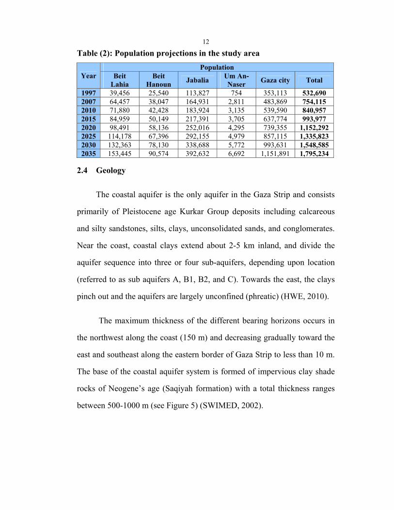
12
Table (2): Population projections in the study area
The study area forms about 30% of the total area of Gaza Strip. It is
distributed between built-up areas (26%); agricultural lands (56%), open
areas (18%).A land use map of the study area is shown in Figure 6 for the
year 1998.
The types of crops planted in the study area include fruits, citrus,
flowers, vegetables and rain-fed crops. Table 3 shows the agricultural
production areas.
14
Figure (6): Land use distribution of the study area
(Source: the database of the PWA, 1998)
Table (3): Agricultural production areas (Hectares*) in North Gaza Item North Gaza
Vegetable 1347.4
Rained crops 861.5
Flowers 9.0
Citrus 2379.7
Fruit 1541
Total 6139
* : 1 hectare =10 dunums (Source: Assessment of land based pollution sources, EQA, 2001)
2.6 Climate
As in Gaza Strip the summers are dry with a short mild rainy season.
The mean temperature varies between 12-14 C° in January to 26-28 C° in
June. The average annual rainfall is about 250 mm/yr, so the recharge
Almond Built-up area Citrus Dates Field crops Fruits Grapes Greenhouse Horticulture Olives Open area Settlements Vegetables
15
volume is about 27 MCM/yr based on 2009/2010 rainfall data. The average
annual potential evaporation is about 1400 mm/yr (SWIMED, 2002).
Figure 7 presents the average annual rainfall data of the study area
obtained from 30 year records from 1980 to 2010.
0
50
100
150
200
250
300
350
400
Distribution of Rainfall (mm)
1980/1981
1982/1983
1984/1985
1986/1987
1988/1989
1990/1991
1992/1993
1994/1995
1996/1997
1998/1999
2000/2001
2002/2003
2004/2005
2006/2007
2008/2009
T ime (Years)
Figure (7): The average annual rainfalls of the study area (1980-2010)
(Source: MoA Reports)
2.7 Existing Water Problems in Gaza Strip
Gaza Strip faces serious problems with seawater intrusion due to over
pumping, as well as aquifer contamination from agricultural and domestic
wastes (SWIMED, 2002).
Figure 8 depicts the contour map for groundwater levels for the study
area with clear appearance of the negative levels due to over pumping.
16
1 0 1 2 Kilom eters
Figure (8): Steady state groundwater level contour map for the study area (Source: PWA, EMCC report 2006)
Tap water in Gaza Strip is known in general to be very salty and
undrinkable. Poor groundwater quality can also be attributed to pollution
from wastewater seepage and the infiltration of agricultural fertilizers
according to a World Bank Report released in April 2009 (IRIN, 2009).
In addition to the previous problems, Gaza’s wastewater
infrastructure causes a true problem since they are provides partial and
intermittent water treatment, so most of sewage goes raw to lagoons and
the sea as shown in Figure 9, or seeps through the soil and reaches the
aquifer, according to the World Bank report (2009).
17
(1) (2) Figure (9): Wastewater problems (1): A sewage lagoon next to a sewage pumping station in Beit Lahia (2): Discharge of untreated wastewater into the sea from the existing Rafah Wastewater Treatment Plant, March 2009
2.8 Water Balance
The two largest components of the water balance are municipal and
agricultural well abstraction. These exceed natural inflows (rainfall
recharge and lateral inflow) therefore the present net aquifer balance is
negative (water deficit). Table 4 and Table 5 summarize the recent
groundwater balance for Gaza Strip and the study area, respectively.
Table (4): Water balance for hydrological year 2008/2009 for Gaza Strip, (Source: HWE, 2010)
flow from septic tanks and networks leakage and inappropriate design of
wastewater treatment plant. All these conditions beside the lateral inflow of
brackish groundwater from the east, leads to accelerate salinization of this
coastal aquifer with chloride, Chloride concentrations in municipal wells in
2009 are shown in Figure10.
Figure (10): Chloride concentration of domestic municipal wells in the study area for year 2009 (Source: PWA reports, 2009)
The WHO drinking chloride limit is 250 mg/l. From Figure 10 it is
clearly that about one half of the wells of the study area exceeded the
maximum limit.
20
Sources of high chloride content have been determined to be
seawater intrusion, lateral flow of brackish water from east and the up-
coning of the brine water from the base of the aquifer.
Most municipal drinking wells in Gaza show nitrate levels in excess
of the WHO drinking water standard of 50 mg/l. Figure 11 shows that
nitrate concentration of 87% of the wells is exceeding the WHO drinking
limit. The main sources for that are domestic sewage effluent and
fertilizers. In contrast to salinity, groundwater flowing from east has
relatively low nitrate levels (PWA, 2009).
Figure (11): Nitrate concentration of domestic municipal wells in the study area for year 2009 (Source: PWA reports, 2009)
2.11 Demand Components
The principal water demand sectors in the study area are the
municipal, industrial, and agricultural sectors. The municipal and industrial
demands are expected to become doubled by the end of the study period,
21
while no increase in agricultural demand is expected since there is no
expansion in the agricultural lands is expected to take place.
Table 6 shows the water demands for all sectors in the study area for
year 2009.
Table (6): Summary of total water demand for all sectors for 2009 in the study area, (Source: PWA reports, 2009)
Item Demand (MCM)
Number of Wells
Municipal & Industrial Water Demand 62.8 52
Agricultural Water Demand 28.9 1002 Total Water Demand 91.7
2.12 Future Municipal Water Needs
The projections of water needs are estimated based on the WHO
standards of 100 L/c/d as a minimum water consumption rate and 150 L/c/d
as an average domestic water consumption. Other consumption rates
including commercial, industrial and livestock consumption rates are
projected as a percentage of the municipal and industrial water needs
(MAS, 2009). A summary of these target consumption rates are shown in
APPENDIX A Table A5.
22
CHAPTER THREE
LITERATURE REVIEW
23
3.1 Introduction
There are many studies of groundwater flow models to help
understand and predict the behavior of fresh and saline groundwater's under
a certain type of exploitation. These studies were important to the
management of groundwater. Seawater intrusion problems have been
solved by using different methods, ranging from the basic Ghyben-
Herzberg principle with the sharp interface models to the more
sophisticated theories with the solute transport models such as SEAWAT
which take into account variable densities. The groundwater flow model is
always a part of any model concerned with the movement of salt-fresh
water interface and/or solute transport, whereas the solute transport model
is necessary for solving most of the groundwater quality problems (Thuan,
2004).
3.2 SEAWAT Application
Qahman (2004) analyzed the major-recent and (desired) future trends
in water availability in Gaza Strip with a special focus on seawater
intrusion and groundwater recovery for Gaza coastal aquifer. He applied
MODFLOW to quantify the availability of groundwater considering the
regional aquifer system and ultimately to predict the long-term
groundwater behavior and the corresponding perennial yield under various
strategies. The main objectives of his study was to determine a perennial
yield pumping and to determine the movement of fresh/saline water
24
interface and the corresponding threat to both freshwater storage and
deterioration of water quality.
The study of Qahman (2004) used MODFLOW to set steady and
transient multiple aquifer simulation models that can be used for the
assessment of groundwater availability and simulation of groundwater
development scenarios. A three dimensional modeling approach is selected
to represent the conceptual model of the Gaza Strip. Model results indicate
that most of the seawater intrusion is happened to the north of Gaza city
and also near Khan-Younis city in the south. It is estimated that seawater
intrusion near Jabalia at year 2003 may extend about 2 Km inland in sub
aquifer B, and up to 3 Km in sub aquifer C.
Qahman and Larabi (2005) assessed numerically the seawater
intrusion in Gaza Strip, applying SEAWAT. Simulation results indicate
that the proposed schemes successfully simulate the intrusion mechanism.
Two pumpage schemes were designed to use the model for prediction of
the future changes in groundwater levels and solute concentrations over a
planning period of 17 years. The results show that seawater intrusion would
worsen in the aquifer if the current rates of groundwater pumpage continue.
The alternatives are to moderate pumpage rates from water supply wells far
from the sea shore and to increase the aquifer replenishment by
encouraging the implementation of suitable solutions like artificial recharge
in order to control seawater intrusion and reduce the current rate of decline
of the water levels.
25
Alzraiee and Durnford (2009) used SEAWAT to simulate the
seawater intrusion in Gaza Coastal Aquifer. The model was used to
determine the extent by which seawater intrusion impacts the groundwater
water quality within the next 10 years. The model was also used to
determine the feasibility of different management scenarios in the future.
The first scenario was the no-action scenario that simulates the
continuation of the current situation for the next 10 years. The second
scenario was to investigate the impact of importing water from the West
Bank via a pipeline. The third scenario was the impact of the installation of
injection wells line along the coast as barrier to the intrusion.
Masterson (2004) simulated interaction between freshwater and
seawater and effects of changing groundwater pumping, recharge
conditions and sea level change at Lower Cape Cod aquifer system,
Massachusetts. SEAWAT was used to assist in the analysis of freshwater
and seawater flow. Model simulations were used to determine water
budgets, flow directions, and the position and movement of the
freshwater/seawater interface. The depth to the freshwater/seawater
interface varies throughout the study area and is directly proportional to the
height of the water table above sea level. Simulated increases in sea level
appear to increase water levels and stream flows throughout the Lower
Cape Cod aquifer system, and yet decrease the depth to the
freshwater/seawater interface. The resulting change in water levels and in
the depth to the freshwater/seawater interface from sea level rise varies
throughout the aquifer system. Pumping from large-capacity municipal-
26
supply wells increases the potential for effects on surface-water bodies,
which are affected by pumping and wastewater-disposal locations and
rates.
Praveena and Aris (2009) presented a case study of groundwater
responses towards the climate change and human pressures in Manukan
Island, Malaysia. SEAWAT was used for the simulations of six scenarios
representing climate change and human pressures showed changes in
hydraulic heads and chloride concentrations. In general, reduction in
pumping rate and an increase in recharge rate are capable to restore and
protect the groundwater resources in Manukan Island. Thus, for
groundwater management options in Manukan Island, scenario 2 is capable
to lessen the seawater intrusion into the aquifer and sustain water resources
on a long-term basis.
Langevin and Mausman (2008) used SEAWAT to predict the extent
rate of saltwater intrusion at Biscayne aquifer of Broward County, Florida,
in response to various sea level rise scenarios using SEAWAT. Until the
date of their study (2008) there are no reported quantitative evaluations of
seawater intrusion in southern Florida in response to sea-level rise. Three
simulations were performed with varying rates of sea level rise. For the
first simulation, the slowest sea level rise was specified at a rate of 0.9
mm/yr, estimated by IPCC. After 100 years, the 250 mg/L chloride moved
inland by about 40 m. For the next simulation, sea level rise was specified
at 4.8 mm/yr. For this moderate rate of sea level rise, the 250 mg/L moved
27
inland by about 740 m after 100 years. For the fastest rate of sea level rise
estimated by IPCC (8.8 mm/yr), the 250 mg/L moved inland by about 1800
m after 100 years.
As furnished in the past studies, this research deals with the climate
change impacts on seawater intrusion using SEAWAT. These impacts are
sea level rise using the maximum value 5.9 mm/yr that was predicted by
IPCC for the Mediterranean region, in addition to recharge and pumping
rates variability. The outcomes of these studies highlighted the in-land
seawater intrusion and the intrusion rates in addition to the expected
increase or decrease in chloride concentration at different wells locations
28
CHAPTER FOUR
CLIMATE CHANGE - A GENERAL BACKGROUND
29
4.1 Definition of Climate Change
Climate change is “a change of climate which is attributed directly
or indirectly to human activities that alter the composition of the global
atmosphere and which is in addition to natural climate variability observed
over comparable time periods” (Pe’er and Safriel, 2000).
The average temperature of the globe has changed over the past
century due to an increase in concentrations of greenhouse gases, mainly
carbon dioxide (CO2), nitrous oxide (N2O) and methane (CH4) (Pe’er and
Safriel, 2000).
4.2 Impacts of Climate Change
The consequences of increasing temperatures, changing patterns of
precipitation, and sea level rise will affect all aspects of the Earth system
(IPCC 2007a; 2007b). The challenges faced by humans at the turn of the
21st century (poverty, disease, conflict, environmental degradation, and so
on) may be exacerbated by climate change. In short, the implications of
climate change are serious. Climate change can be considered as the
biggest environmental threat in human history and as the defining human
development challenge for the 21st century (IPCC 2007b; UNDP 2008).
4.3 Predictions of Climate Change for the Middle East
In a region already considered the world’s most water scarce, where
demand for water already outstrips supply in many places; climate models
30
are broadly predicting a hotter, drier and less predictable climate (Alpert,
2008).
By the middle of the century, the region is expected to get hotter
across all seasons models predict an increase of between 2.5 to 3.7°C in
summer, and 2.0 to 3.1°C in winter (see Figure 12 and 13). (Cruz, 2007),
Higher temperatures will change where rain falls, how much of it falls and
how often it falls. It will also result in a global increase in sea levels; the
region will get drier, with significant rainfall declines in the wet season
outweighing slight increases during the drier summer months (Cruz, 2007).
Meanwhile, the distribution of rains will change (moving to the north). The
weather is also likely to become more unpredictable, with the region
experiencing an increase in extreme rainfall events (Alpert, 2008).
31
Figure (12): RCM projections of temperature changes (ºC) across the Gulf region for 2020s, 2040s and 2070s relative to the 1990s
Figure (13): RCM projections of precipitation changes (%) across the Gulf region for 2020s, 2040s and 2070s relative to the 1990s
4.4 Predictions of Climate Change for the Mediterranean
Regarding the precipitation projection, the RCM (Regional Climate
Models) results for 2071–2100 compared to 1961–1990 show large
32
differences between scenarios A2 and B2 emission scenarios (1) (Figure 14).
The black box in the figure is centered over Palestine and the Jordan River
basin. In A2, most of the Eastern Mediterranean (EM) shows rainfall
reduction of about 15–75 mm for DJF (December, January and February),
which is equivalent to drops of about 10–30%. Model results indicate that
groundwater recharge is unlikely to decrease by more than 10% until the
2050s. The DJF period covers most of the annual rain in the EM, and
realistically reflects the annual rainfall changes. In scenario B2, however
rainfall reductions are significantly lower and are of about 0–15% in total
rainfall, while over most of Turkey significant rainfall increases are
noticed. The predicted rainfall changes in B2 are similar to those observed
over the EM during the recent decades (e.g., Alpert, 2004; IPCC, 2001) that
also show larger precipitation decreases over the NE Mediterranean and
some small increases over the SE Mediterranean (Alpert et al, 2008).
(1) The near surface air temperature differences from 2071–2100 compared to 1961–1990 are based on the RCM results for two International Panel for Climate Change (IPCC) emission scenarios A2 and B2. The A2 scenario assumes a significant increase of the GHG concentration whereas the B2 is based on less extreme estimates
33
Figure (14): The winter (DJF) predicted change in the mean seasonal precipitation (mm). Differences are between A2 and B2 scenarios (2071–2100) as compared to the control run (1961–1990) values over the EM, and are based on the RCM runs.
Results of regional climate modeling performed at the International
Centre for Theoretical Physics, (Trieste, Italy) are analyzed for the
Mediterranean region. It is found that the average temperature over the
Mediterranean area has increased by 1.5–4°C in the last 100 years. The
temperature in the years 2071–2100 according to the A2 and B2 scenarios
for (2071–2100) as compared to the control run (1961–1990) values over
the EM, and are based on the RCM runs, as shown in Figure 15 are
predicted to increase by about 4°C and 6°C, respectively over Northern
Palestine in comparison with the control run for 1961–1990 (Alpert et al,
2008).
34
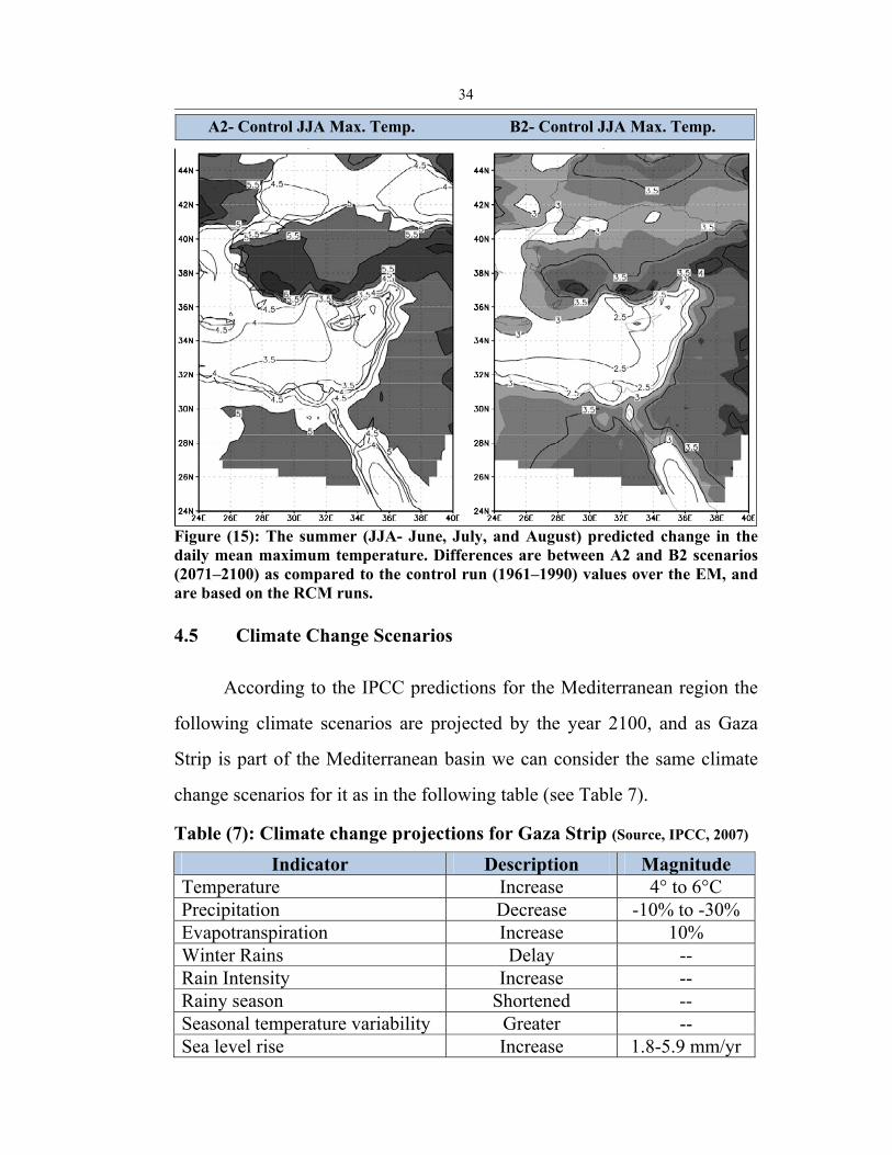
Figure (15): The summer (JJA- June, July, and August) predicted change in the daily mean maximum temperature. Differences are between A2 and B2 scenarios (2071–2100) as compared to the control run (1961–1990) values over the EM, and are based on the RCM runs.
4.5 Climate Change Scenarios
According to the IPCC predictions for the Mediterranean region the
following climate scenarios are projected by the year 2100, and as Gaza
Strip is part of the Mediterranean basin we can consider the same climate
change scenarios for it as in the following table (see Table 7).
Indicator Description Magnitude Temperature Increase 4° to 6°C Precipitation Decrease -10% to -30% Evapotranspiration Increase 10% Winter Rains Delay -- Rain Intensity Increase -- Rainy season Shortened -- Seasonal temperature variability Greater -- Sea level rise Increase 1.8-5.9 mm/yr
A2- Control JJA Max. Temp. B2- Control JJA Max. Temp.
35
4.5.1 Temperature
Price et al. (1999) observed an approximate 1oC/100yr rise in annual
mean temperature in Cyprus. Alpert et al. (unpublished data) observed the
same warming trend in Cyprus, as well as in Italy and Spain. A relatively
moderate increase in air temperature was measured in cities of the
Mediterranean, primarily in winter and less in the autumn and spring
(Maheras and Kutiel 1999; Kutiel and Maheras 1998). Most of the increase,
however, was measured in cities undergoing urbanization (Kutiel and
Maheras 1998).
4.5.2 Precipitation
Rainfall measurements at different stations in the Mediterranean
region show similar declines in most regions of the basin (Paz et al. 1998a).
High correlation between changes in vegetation and changes in sea level
during the last decade in the Middle East suggests that the trend of
decreasing precipitation in the Middle East may be attributed to global
warming (Issar 1995).
Increased surface runoff will reduce aquifer recharge, transport
dissolved pollutants to waters reservoirs, increase flash floods during peak
water flows and damaging human structures and crops (Pe’er and Safriel,
2000).
36
4.5.3 Sea level rise
Climate change has a great direct effect on seawater intrusion
because it leads to a rise in the global sea level and intrusion of seawater
into the coastal aquifer and this will further damage groundwater. The
increase in the global temperature will warm the land surface, oceans and
seas. This warming will decrease the atmospheric pressure, which will in
turn lead to the increase of the water level in the oceans and seas. This rise
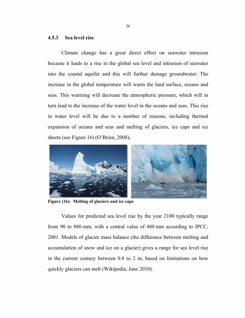
in water level will be due to a number of reasons, including thermal
expansion of oceans and seas and melting of glaciers, ice caps and ice
sheets (see Figure 16) (O’Brien, 2008).
Figure (16): Melting of glaciers and ice caps
Values for predicted sea level rise by the year 2100 typically range
from 90 to 880 mm, with a central value of 480 mm according to IPCC,
2001. Models of glacier mass balance (the difference between melting and
accumulation of snow and ice on a glacier) gives a range for sea level rise
in the current century between 0.8 to 2 m, based on limitations on how
quickly glaciers can melt (Wikipedia, June 2010).
37
According to the greenhouse gas emissions scenario, sea levels at the
Mediterranean Sea are forecasted by the IPCC to rise at least 18 to 38 cm
and as much as 26 to 59 cm by 2100 (Mason et al. 2009).
In Palestine, a local assessment of sea level rise found only a 5 cm to
10 cm rise since 1960. Tectonic movements in the eastern Mediterranean,
measured through tide-gauge measurements in Haifa indicate an uplift of
+2.8 mm/yr (about 3cm in a decade) (Jelgersma and Sestini 1992). Hence,
long-term measurements are needed to accurately assess local changes in
sea level in Palestine (Issar 1995).
38
CHAPTER FIVE
SEAWATER INTRUSION
39
5.1 General Background and Definitions
Seawater intrusion is the movement of seawater into fresh water
coastal aquifers due to natural processes or human activities. Seawater
intrusion is caused by decreases in groundwater levels or by rises in
seawater levels. When you pump out fresh water rapidly, you lower the
height of the freshwater in the aquifer forming a cone of depression.
According to Ghyben-Herzberg theory the salt water rises 40 feet for every
1 foot of freshwater depression and forms a cone of ascension. Intrusion
can affect the quality of water not only at the pumping well locations, but
also at other well locations, by increasing salinity of the groundwater; see
Figure 17 (Lenntech, 2009).
(a) (b)
Figure (17): (a): Clarifications of Ghyben-Herzberg theory, (b): effect of pumping into freshwater/seawater interface, (Source Lenntech, 2009)
In coastal aquifers, an interface exists between fresh groundwater
flowing toward the sea and saline groundwater. Across the interface, the
fluid density may increase from that of freshwater (about 1,000 kg/m3) to
that of seawater (about 1,025 kg/m3), an increase of about 2.5 percent.
40
An understanding of variable-density groundwater flow is important in
many types of studies of coastal aquifers, such as studies of seawater
intrusion, contaminated site remediation and fresh groundwater discharge
into oceanic water bodies (Guo and Langevin, 2002).
5.2 Consequences and Assessments
Salinization of groundwater is considered a special category of
pollution that threatens groundwater resources, because mixing of a small
quantity of seawater with groundwater makes freshwater unsuitable and
can result in abandonment of freshwater supply (Hany, 2009).
In coastal areas the aquifers are in hydraulic contact with the sea, and
under normal conditions freshwater flows into the sea. However, over-
pumping may result in inversion of the groundwater flow from the sea
towards the inland, causing seawater intrusion. Therefore, seawater
intrusion should be prevented or at least controlled to protect groundwater
resources. In general, control can be achieved by maintaining an
appropriate balance between water being pumped from the aquifer and the
amount of water recharged to the aquifer. Sea level rise also threatens
groundwater in coastal aquifers because it imposes an additional pressure
head from the sea side which promotes the movement of seawater into the
aquifer (Hany, 2009).
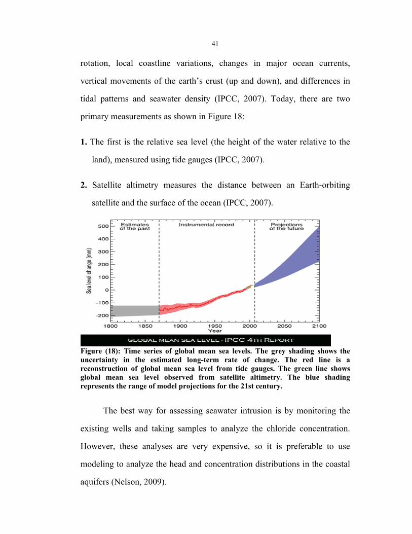
5.3 How to Assess Seawater Intrusion?
A complication in measuring sea level, is that the sea level does not
rise by the same amount all over the globe due to the effects of the earth’s
41
rotation, local coastline variations, changes in major ocean currents,
vertical movements of the earth’s crust (up and down), and differences in
tidal patterns and seawater density (IPCC, 2007). Today, there are two
primary measurements as shown in Figure 18:
1. The first is the relative sea level (the height of the water relative to the
land), measured using tide gauges (IPCC, 2007).
2. Satellite altimetry measures the distance between an Earth-orbiting
satellite and the surface of the ocean (IPCC, 2007).
Figure (18): Time series of global mean sea levels. The grey shading shows the uncertainty in the estimated long-term rate of change. The red line is a reconstruction of global mean sea level from tide gauges. The green line shows global mean sea level observed from satellite altimetry. The blue shading represents the range of model projections for the 21st century.
The best way for assessing seawater intrusion is by monitoring the
existing wells and taking samples to analyze the chloride concentration.
However, these analyses are very expensive, so it is preferable to use
modeling to analyze the head and concentration distributions in the coastal
aquifers (Nelson, 2009).
42
There is a wide range of commercial and public domain computer
codes that can be used to simulate variable-density groundwater flow. For
example, the U.S. Geological Survey (USGS) offers the finite-element
SUTRA code (Voss, 1984) and the finite-difference HST3D (Kipp, 1997)
and MOCDENSE (Sanford and Konikow, 1985) codes. These codes
contain powerful options for simulating a wide range of complex problems
(Guo and Langevin, 2002).
With the increase in demand for fresh groundwater resources, the
number of studies that require explicit representation of fluid density
variation has increased. Many of these studies focus on seawater intrusion
issues in coastal areas. USGS investigators have developed expertise in
applying the SEAWAT computer program to a wide variety of
groundwater problems which is a MODFLOW-based computer program
(Langevin, 2009).
MODFLOW is the U.S. Geological Survey modular finite-difference
flow model, which is a computer code that solves the groundwater flow
equation. The program is used by hydrogeologists to simulate the flow of
groundwater through aquifers.
5.4 SEAWAT Concept
SEAWAT was designed to simulate three-dimensional, variable-
density groundwater flow in porous media coupled with multi-species
solute transport. The program has been used for a wide variety of
groundwater studies related to seawater intrusion. SEAWAT is relatively
43
easy to apply because it uses the familiar MODFLOW structure. SEAWAT
is a public domain computer program distributed free of charge by the U.S.
Geological Survey. SEAWAT can be downloaded from the following
SEAWAT reads and writes standard MODFLOW and MT3DMS (1)
data sets, although some extra input may be required for some SEAWAT
simulations (Guo and Langevin, 2002).
SEAWAT is based on the concept of freshwater head, or equivalent
freshwater head, in a saline groundwater environment. A thorough
understanding of this concept is required in developing the equations of
variable-density groundwater flow as used in the SEAWAT program and in
interpreting calculated results, (Guo and Langevin, 2002). In order to
understand the equivalent freshwater head, two piezometers open to a given
point, N, in an aquifer containing saline water are shown in Figure 19.
Piezometer A contains freshwater and is equipped with a mechanism
that prevents saline water in the aquifer from mixing with freshwater in the
piezometer, while still allowing the piezometer to respond accurately to the
pressure at point N. Piezometer B contains water identical to that present in
the saline aquifer at point N. The height of the water level in piezometer A
above point N is hf. The freshwater head at point N is the elevation of the
water level in piezometer A above datum, and thus is given by: (Guo and
Langevin, 2002)
(1) A modular three-dimensional multi species transport model for simulation of advection, dispersion and chemical reactions of contaminants in groundwater systems.
44
where: hf is the equivalent freshwater head [L] P is the pressure at point N [ML-1T-2] ρf is the density of freshwater [M/L3] g is the acceleration due to gravity [L/T-2] Z is the elevation of point N above datum [L]
Figure (19): Two piezometers, one filled with freshwater and the other with saline aquifer water, open to the same point in the aquifer
(Source: Guo and Langevin, 2002).
5.4.1 SEAWAT procedure
The source code for SEAWAT was developed by combining
MODFLOW and MT3DMS into a single program that solves the coupled
flow and solute-transport equations (Guo and Langevin, 2002).
MODFLOW solves groundwater flow equation by solving for each
time step, cell by cell flow is calculated from the fresh water head gradients
and relative density difference terms, and results will give velocities and
f
f
(1)
45
heads. While MT3DMS solves the solute transport equation by using solute
transport equation based on previous MODFLOW results and repeated
until stress period and simulation is complete. The numerical methods used
by the MT3DMS program to simulate solute transport in a constant density
flow field are directly used in SEAWAT to simulate solute transport in a
variable-density flow field (Guo and Langevin, 2002).
5.4.2 Governing Equations
Simulation of groundwater flow is performed by numerically solving
the groundwater flow and solute-transport equations. The governing flow
and transport equations in SEAWAT are as in Equations 2 and 3. The
SEAWAT package is very flexible and user friendly. This package has
been very useful to simulate variable density flow through complex
geology. One advantage of SEAWAT is that it uses MT3DMS to represent
solute-transport (Guo and Langevin, 2002).
The groundwater flow equation can take many forms depending on
the assumptions that are valid for the problem of interest. In most cases, it
is assumed that the density of groundwater is spatially and temporally
constant. To simulate groundwater flow in coastal environments, the
assumption of constant density is not valid because seawater contains a
higher concentration of dissolved salts than rainfall, which is the primary
source for aquifer recharge. Fluid density is a function of dissolved salt.
The density difference between fresh groundwater and seawater can greatly
affect groundwater flow patterns. Accordingly, for that the groundwater
46
flow equation used in the present study does not assume that groundwater
density is constant (Guo and Langevin, 2002).
The groundwater flow equation is as follows: (Guo and Langevin,
2002)
where:
Xi ith orthogonal coordinate Kf equivalent freshwater hydraulic conductivity (L/T) Sf equivalent freshwater specific storage (1/L) hf equivalent freshwater head (L) t time (T) θ effective porosity (dimensionless) ρ is density of freshwater [M/L3] ρs is density of sources and sinks [M/L3] qs volumetric flow rate of sources and sinks per unit volume of aquifer
(1/T) The transport equation is as follows: (Guo and Langevin, 2002)
where:
Ck dissolved concentration of species k [M/L3]. Ck
s concentration of the source or sink for species k [M/L3] Di is the dispersion coefficient [L2/T] qs is the volumetric flux of a source or sink [T-1] Rn the chemical reaction term (ML3/T)
Dispersion is a physical process that tends to ‘disperse’, or spread,
the contaminant mass in the X, Y and Z directions along the advective path
(2)
(3)
47
of the plume, and acts to reduce the solute concentration. Dispersion is
caused by the tortuosity of the flow paths of the groundwater as it travels
through the interconnected pores of the soil.
The Dispersion inputs in Visual MODFLOW used the Longitudinal
Dispersivity values in the model while MT3D calculates the Dispersion
tensor for the mass transport model using the following parameters:
• Longitudinal Dispersivity for each transport grid cell
• Ratio of Horizontal to Longitudinal Dispersivity for each layer = 0.1
• Ratio of Vertical to Longitudinal Dispersivity for each layer = 0.001
• Molecular Diffusion Coefficient for each layer = 0 m2/d
The source for species in this research is the salt, which is didn't
decay or degradation for that no kinetic reactions are used.
48
CHAPTER SIX
DEVELOPMENT OF THE SEAWAT MODEL FOR THE NORTH GAZA
AREA
49
6.1 Introduction
This research deals with the groundwater resources assessment and
future forecasting under various scenarios. These scenarios are related to
human stresses and climate changes in order to increase our understanding
of the seawater intrusion in the North Gaza aquifer.
The basic groundwater flow model for this study was developed
based on the MODFLOW model which was prepared by PWA and the
EMCC for the purpose of study the environmental impact assessment for
Beit Lahia WWTP.
6.2 Basic Groundwater Flow Model
The model domain encloses an area of 391 km2 (1) in the northern
part of Gaza Strip. Figure 4 in Chapter 2 shows the selected model domain
which is part of the coastal aquifer. The model domain originally consists
of 78 rows, 88 columns and one layer. The horizontal grid is divided into
uniform cells with size of 200x200m.
For modeling purposes, the hydrologic year consists of a winter
season from October to March and a summer season from April to
September. Simulations started from the hydrologic year 2000.
The model boundaries can be described as follows (see Figure 20):
• West: Constant head boundary with zero head.
(1): This area includes additional area outside the North Gaza borders. The reason for expanding
the model domain beyond the study area is to minimize the effects of model boundaries in the
central part of the model.
50
• East: Constant head boundary with variable head between 11 to 18
meters. The eastern boundary was selected to minimize the boundary
effects on the areas inside the aquifer (there is a considerable lateral
flow from east to west at the borders with Gaza), the best selection
was the outcrop of the coastal aquifer 10-15 Km east of Gaza. Near
this line there are few points were the head is available, entered to the
model cell by cell with a range between 11-18 m.
• North and South: Considered as no-flow boundary: Since the contour
lines of the water table elevations of Gaza Coastal aquifer are parallel
to the eastern and western boundaries (as shown in Figure 8, Section
2.7), then the flow will parallel to the northern and southern
boundaries of the model domain and this can be considered as a no-
flow boundary.
Figure (20): Model boundaries and grid
Constant head between 11-18m
Constant head (Sea) =0
51
The lower boundary of the model consists of Saqiyah surface (see
Figure 21).
Figure (21): Bottom of the aquifer and the ground surface elevation
6.2.1 Recharge Components
The recharge was estimated based on 1999-2000 data. The net
recharge for the study area is comprised of recharge from rain, irrigation
return flow, water networks losses, wastewater leakages, existing treatment
plants and recharges basins, and recharge from treated wastewater
irrigation in the Israeli side of the model domain.
A total of 27 recharge zones were considered for the MODFLOW
input. Each zone carries a different value based on the annual and seasonal
recharge values (see Figure 22).
Upper elevation (ground surface)
Lower elevation
Water Table
52
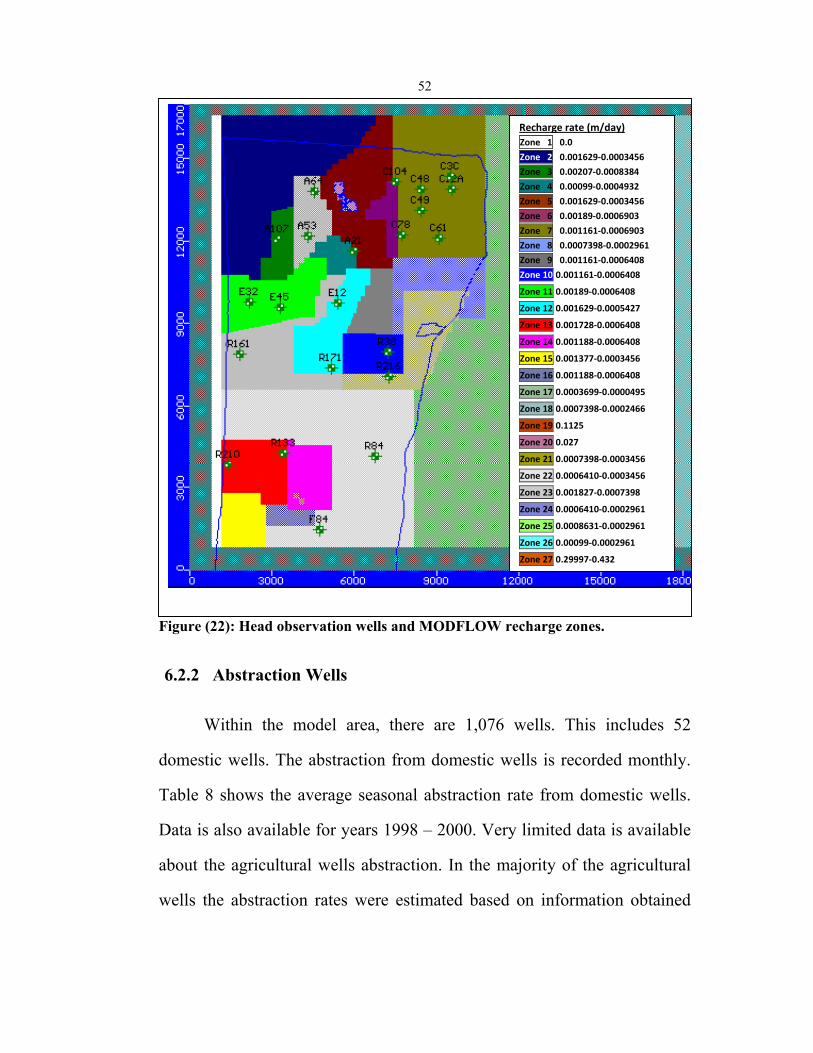
Figure (22): Head observation wells and MODFLOW recharge zones.
6.2.2 Abstraction Wells
Within the model area, there are 1,076 wells. This includes 52
domestic wells. The abstraction from domestic wells is recorded monthly.
Table 8 shows the average seasonal abstraction rate from domestic wells.
Data is also available for years 1998 – 2000. Very limited data is available
about the agricultural wells abstraction. In the majority of the agricultural
wells the abstraction rates were estimated based on information obtained
Recharge rate (m/day) Zone 1 0.0
Zone 2 0.001629‐0.0003456
Zone 3 0.00207‐0.0008384
Zone 4 0.00099‐0.0004932
Zone 5 0.001629‐0.0003456
Zone 6 0.00189‐0.0006903
Zone 7 0.001161‐0.0006903
Zone 8 0.0007398‐0.0002961
Zone 9 0.001161‐0.0006408
Zone 10 0.001161‐0.0006408
Zone 11 0.00189‐0.0006408
Zone 12 0.001629‐0.0005427
Zone 13 0.001728‐0.0006408
Zone 14 0.001188‐0.0006408
Zone 15 0.001377‐0.0003456
Zone 16 0.001188‐0.0006408
Zone 17 0.0003699‐0.0000495
Zone 18 0.0007398‐0.0002466
Zone 19 0.1125
Zone 20 0.027
Zone 21 0.0007398‐0.0003456
Zone 22 0.0006410‐0.0003456
Zone 23 0.001827‐0.0007398
Zone 24 0.0006410‐0.0002961
Zone 25 0.0008631‐0.0002961
Zone 26 0.00099‐0.0002961
Zone 27 0.29997‐0.432
53
from the Ministry of Agriculture about irrigated areas, crop patterns, and
crop water requirements (M&E, 2000).
22 wells were selected as head observation wells for the model
regional calibration (Figure 21). The selection was based on the availability
of good hydrograph for these wells. More details are presented in the
calibration section.
Table (8): Average Seasonal abstraction rates from the Municipal wells, (Source: PWA Data 2001-2003)
Abstraction period
QS 2001
QW 2001
QS 2002
QW 2002
QS 2003
QW 2003
Total pumping
rates (m3/day)
113,924 96,145 117,710 100,887 120,010 102,163
QS = average abstraction rate from April to September (m3/day) QW = average abstraction rate from October to March (m3/day)
6.2.3 Simulation Period
The simulation period for the basic groundwater flow model was
8,030 days to reflect a 22 years of time starting from the hydrologic year
2000 until 2022.
6.2.4 Steady State Model Calibration
Data from year 1998 to 2000 was used for the steady state
calibration. The modeled water level was then calibrated based on year
2000. Figure 8 in Chapter 2 shows the steady state water level contour map
for the year 2000. In general, the modeled contour map shows a good
54
agreement with the previous modeling results for instance the (CAMP
project) for the same period.
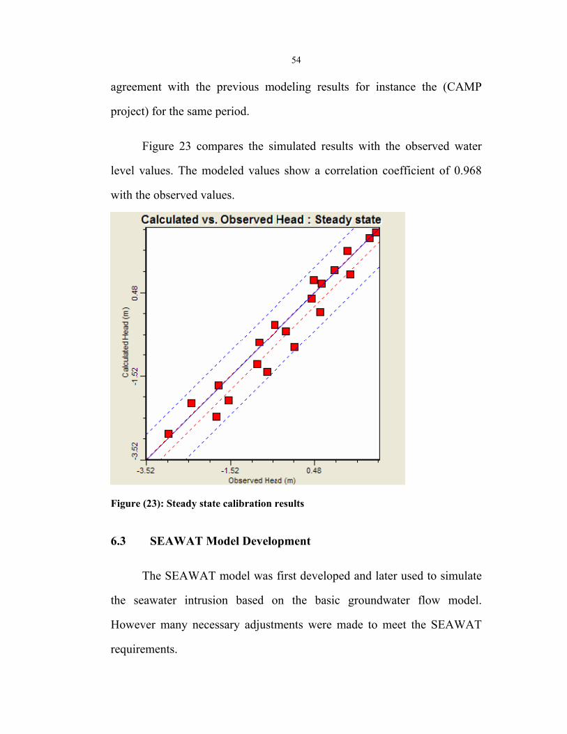
Figure 23 compares the simulated results with the observed water
level values. The modeled values show a correlation coefficient of 0.968
with the observed values.
Figure (23): Steady state calibration results
6.3 SEAWAT Model Development
The SEAWAT model was first developed and later used to simulate
the seawater intrusion based on the basic groundwater flow model.
However many necessary adjustments were made to meet the SEAWAT
requirements.
55
The North Gaza aquifer was vertically discretized into ten layers to
better represent the vertical variability in salinity in the study area using the
developed SEAWAT model.
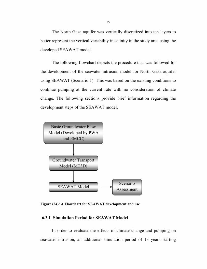
The following flowchart depicts the procedure that was followed for
the development of the seawater intrusion model for North Gaza aquifer
using SEAWAT (Scenario 1). This was based on the existing conditions to
continue pumping at the current rate with no consideration of climate
change. The following sections provide brief information regarding the
development steps of the SEAWAT model.
Figure (24): A Flowchart for SEAWAT development and use
6.3.1 Simulation Period for SEAWAT Model
In order to evaluate the effects of climate change and pumping on
seawater intrusion, an additional simulation period of 13 years starting
Basic Groundwater Flow Model (Developed by PWA
and EMCC)
Groundwater Transport Model (MT3D)
SEAWAT Model Scenario
Assessment
56
from 2023 until 2035 was added to the original simulation period (from
2000-2022). As such, the SEAWAT model covers 35 years (from 2000
until 2035).
6.3.2 Boundary Conditions
Constant head cells were assigned along the sea line and the deepest
two layers to the east. Initial concentrations were assigned to the model
according to the following assumptions (Qahman, 2004 (these values had
been used by Israeli Modeling work for Gaza that had been done by Prof.
Sahul Sorik from Ben Gorion University)):
• Constant concentration (western boundary) is 35,000 mg/l
• Constant concentration (eastern boundary, layers 9 and 10) is 700 mg/l
• Initial chloride concentration =102.5 mg/l (equivalent to 0.1 g/Kg)
everywhere except at the specific locations of domestic wells which
are exceeding this value.
• Specific chloride concentrations assigned to each domestic well
location to reflect the actual conditions.
• Recharge concentration was neglected and considered 0 mg/l since the
main scope of the work concentrates on salinity from seawater
intrusion.
The dispersion coefficient was modified everywhere as needed to
reflect the actual situation for salinity inside the model. Initial conditions
57
(heads and concentrations) were specified using the results from a long
term simulation in which the model had reached steady-state flow and
transport conditions.
As there is no available data for the current sea level rise, this
simulation was performed using a present day sea level of zero meters.
During the simulations, a maximum sea level rise of 59 cm/100 yr was
considered as appropriate (IPCC, 2007). Table 9 summarizes the input
parameters for the SEAWAT model.
Table (9): Input parameters for the SEAWAT model
Parameter Value Hydraulic conductivity Kxy 35 m/d Hydraulic conductivity Kz 3 m/d Total porosity 0.35 Effective porosity 0.25 Specific storage 0.00002 m-1 Specific yield 0.15 Longitudinal dispersivity 12 m Horizontal transverse dispersivity 0.1 mVertical transverse dispersivity 0.01m
6.3.3 Calibration of the SEAWAT Model
The SEAWAT model was calibrated for chloride concentration by
entering the available chloride concentrations that recorded for specific
wells by PWA at year 2000, as the initial concentrations, and then the
model was run to get the simulated concentrations at year 2009 which was
compared with PWA observed concentrations for the same year. This was
done for each of the specific well locations to meet with the needed
concentrations at year 2009.
58
In addition to adjustment of the longitudinal dispersivity since it is
the required parameter for SEAWAT simulation as discussed in the
governing equations in Chapter 5.
As shown in see Figure 25 it can be concluded that there is a good
match between the simulated and observed concentrations. The spearman
rank correlation was 96% between the simulated concentrations and the
observed ones as shown in APPENDIX A (A6).
Figure (25): Observed versus Simulated concentration for selected wells for year 2009
59
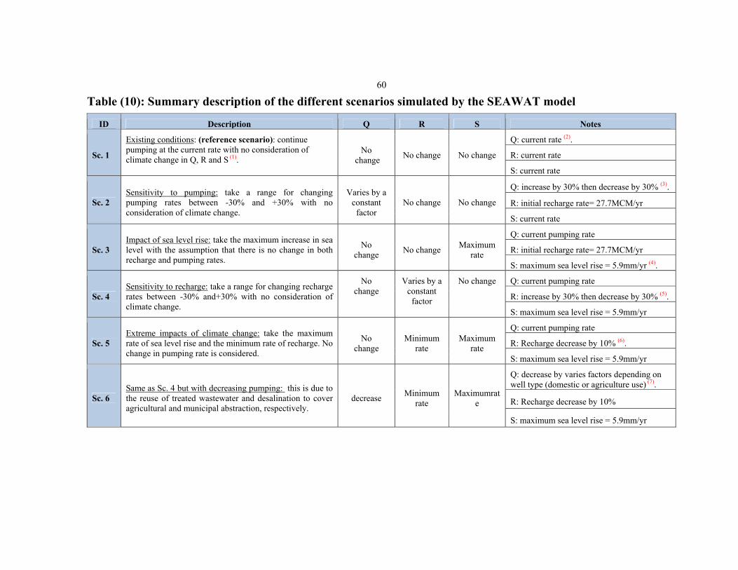
6.4 The Studied Scenarios
The reference scenario considered herein is Scenario 1. The studied
scenarios are listed in Table 10 and are in general based on the IPCC
projections for the Mediterranean coast for the next 25 years along with the
PWA recommendations and projections (especially for scenario 6).
The reference scenario is based on the following assumptions:
Current pumping rate for year 2010 is 91.7 MCM (28.9 MCM for
agriculture, and 62.8 MCM for domestic).
Current annual recharge rate (R) is 27.7 MCM
Current sea level rise (S) is zero
In order to study the sensitivity of the aquifer for these three impacts,
specialized scenarios were simulated for each impact. Scenario 2 considers
the impact of increasing and decreasing pumping rates. Scenario 3
considers the impact of maximum sea level rise. Scenario 4 considers the
impact of increasing and decreasing recharge rates.
60
Table (10): Summary description of the different scenarios simulated by the SEAWAT model
ID Description Q R S Notes
Sc. 1
Existing conditions: (reference scenario): continue pumping at the current rate with no consideration of climate change in Q, R and S (1).
No change No change No change
Q: current rate (2).
R: current rate
S: current rate
Sc. 2 Sensitivity to pumping: take a range for changing pumping rates between -30% and +30% with no consideration of climate change.
Varies by a constant factor
No change No change
Q: increase by 30% then decrease by 30% (3).
R: initial recharge rate= 27.7MCM/yr
S: current rate
Sc. 3 Impact of sea level rise: take the maximum increase in sea level with the assumption that there is no change in both recharge and pumping rates.
No change No change Maximum
rate
Q: current pumping rate
R: initial recharge rate= 27.7MCM/yr
S: maximum sea level rise = 5.9mm/yr (4).
Sc. 4 Sensitivity to recharge: take a range for changing recharge rates between -30% and+30% with no consideration of climate change.
No change
Varies by a constant
factor
No change Q: current pumping rate
R: increase by 30% then decrease by 30% (5).
S: maximum sea level rise = 5.9mm/yr
Sc. 5 Extreme impacts of climate change: take the maximum rate of sea level rise and the minimum rate of recharge. No change in pumping rate is considered.
No change
Minimum rate
Maximum rate
Q: current pumping rate
R: Recharge decrease by 10% (6).
S: maximum sea level rise = 5.9mm/yr
Sc. 6 Same as Sc. 4 but with decreasing pumping: this is due to the reuse of treated wastewater and desalination to cover agricultural and municipal abstraction, respectively.
decrease Minimum rate
Maximumrate
Q: decrease by varies factors depending on well type (domestic or agriculture use) (7).