Applied Mathematical Sciences, Vol. 9, 2015, no. 146, 7269 - 7280

HIKARI Ltd, www.m-hikari.com http://dx.doi.org/10.12988/ams.2015.511715

Numerical Solution of Non-Linear Biharmonic

Equation for Elasto-Plastic Bending Plate

Feda Ilhan

Department of Mathematics

Abant Izzet Baysal University, Bolu, Turkey

Zahir Muradoglu

Department of Mathematics

Kocaeli University, Kocaeli, Turkey

Copyright © 2015 Feda Ilhan and Zahir Muradoglu. This article is distributed under the

Creative Commons Attribution License, which permits unrestricted use, distribution, and

reproduction in any medium, provided the original work is properly cited.

Abstract

A numerical solution for the non-linear boundary value problem of elasto-plastic

bending plate by means of finite difference method is proposed. Test functions, as

defined along this work, are employed for verifying the applicability of the

computer program. Accuracy of the approximate solutions is demonstrated through

the numerical examples.

Keywords: Non-linear biharmonic equation, elasticity, plasticity, deformation,

finite difference method, elasto-plastic plate

1 Introduction

Biharmonic equation plays an important role in different scientific disciplines, but

it is difficult to solve due to the existing fourth order derivatives. They arise in

several areas of mechanics such as two dimensional theory of elasticity and the

deformation of elastic and elasto-plastic plates [1, 2]. Various approaches for the

numerical solution of biharmonic equation have been considered in the literature

over several decades. But these kind of problems are usually obtained through the

use of finite element method which requires the use of nonphysical dissipation.

However, the finite element solution is not as stable as the finite difference solution

which has not only the ease of grid generation but also dissipative character.

7270 Feda Ilhan and Zahir Muradoglu

A general variational approach has been constructed by Hasanov [3] for solving

the non-linear bending problem of elasto-plastic plate by using monotone operator

theory. In this work existence of the weak solution of the non-linear problem in

𝐻2(Ω) Sobolev space is given and by using finite difference method numerical

solution for linear bending problems with various boundary conditions is obtained.

Plate structures are most commonly encountered in analyzing engineering

structures. In recent years, considerable attempts have been made in the

development of numerical methods for the analysis of solid mechanics problems.

The elasto-plastic behavior of plates has been analyzed by several numerical

methods such as the finite element [4, 5], boundary element [6, 7], finite strip [8, 9],

meshless based methods [10, 11] and the others.

The essential purpose of this study is to obtain a numerical solution for the

non-linear biharmonic equation for elasto-plastic bending plate with different

boundary conditions by using finite difference method.

The paper is organized as follows. In section 2 the mathematical model and

governing equations for the non-linear bending problems are represented. In

section 3 finite difference approximation of the problem is derived. In section 4 by

using a test function applicability of the finite difference method which has been

carried out in Matlab is shown and the numerical algorithm and examples related to

the non-linear problem are considered. In section 5 conclusions are given.

2 The mathematical model and governing equations

In this paper, bending problem of the plate which is tailored with an elasto-plastic

and homogeneously isotropic incompressible features is studied. For simplicity, the

plate is supposed to be rectangular. The basic plate equations contain no such shape

restriction, but solutions are most easily determined for rectangular plates and

circular plates. It is assumed that the plate with thickness is placed to the

coordinate system 𝑂𝑥1𝑥2𝑥3 such that the middle surface of the plate is located in

𝑂𝑥1𝑥2 plane. The plate is supposed to be in equilibrium under the action of the

loads applied on the upper surface of the plate in the 𝑥3 axis direction while its

lower surface is free. It is known from the deformation theory of plasticity that

[12, 13] as 𝜔 = 𝜔(𝑥) is the deflection of a point 𝑥 ∈ Ω on the middle surface of the

plate, which is placed in the region Ω = {(𝑥1, 𝑥2) ∈ 𝑅2: 0 ≤ 𝑥𝛼 ≤ 𝑙𝛼 , 𝛼 = 1,2} ,

satisfies the following nonlinear biharmonic equation:

𝐴𝜔 ≡ 𝜕2

𝜕𝑥12 [𝑔(𝜉2(𝜔)) (

𝜕2𝜔

𝜕𝑥12 +

1

2

𝜕2𝜔

𝜕𝑥22 )] +

𝜕2

𝜕𝑥1𝜕𝑥2[𝑔(𝜉2(𝜔))

𝜕2𝜔

𝜕𝑥1𝜕𝑥2]

+𝜕2

𝜕𝑥22 [𝑔(𝜉2(𝜔)) (

𝜕2𝜔

𝜕𝑥22 +

1

2

𝜕2𝜔

𝜕𝑥12 )] = 𝐹(𝑥), 𝑥 ∈ Ω

⊂ 𝑅2 (2.1)

𝐹(𝑥) = 3𝑞(𝑥)/ ℎ3 and 𝑞 = 𝑞(𝑥) is the intensity of the loads applied on the

plate. Boundary conditions which may also be called edge or support conditions

include simply supported, clamped, free and a wide variety of conditions applied

Numerical solution of non-linear biharmonic equation 7271

to certain applications. Though in practice simply supported condition and

especially clamped boundary condition are difficult to enforce this study

specifically exploits these two conditions [14]:

1. Clamped boundary condition

𝜔(𝑥) = 𝜕𝜔

𝜕𝑛(𝑥) = 0 (2.2)

2. Simply supported boundary condition

𝜔(𝑥) = 𝜕2𝜔

𝜕2𝑛= 0 (2.3)

where 𝑛 is the unit outward normal to the boundary 𝜕Ω.

Corresponding to Kachanov's model of elasto-plastic deformation theory for

isotropic homogeneous deformable materials the relation between deviations of the

stress 𝜎𝐷 = {𝜎𝑖𝑗𝐷} and the deformation 휀𝐷 = {휀𝑖𝑗

𝐷} 𝑖, 𝑗 = 1, 2, 3 is described by

the Hencky relation [12, 13]:

𝜎𝑖𝑗𝐷(𝑢) = �̅�(Γ2)휀𝑖𝑗

𝐷(𝑢) (2.4)

Consequently, the relationship between the intensities of the shear stress

�̅� = (0.5𝜎𝑖𝑗𝐷𝜎𝑖𝑗

𝐷)1 2⁄

and the shear strain Γ = (2휀𝑖𝑗𝐷휀𝑖𝑗

𝐷)1 2⁄ is expressed as:

�̅� = �̅�(Γ2) Γ (2.5)

where

Γ2 = 4𝑥32 [(

𝜕2𝜔

𝜕𝑥12 )

2

+ (𝜕2𝜔

𝜕𝑥22 )

2

+ (𝜕2𝜔

𝜕𝑥1𝜕𝑥2)

2

+𝜕2𝜔

𝜕𝑥12

𝜕2𝜔

𝜕𝑥22 ] (2.6)

With the aid of [15] , the dependent variable 𝜉 = 𝜉(𝜔) is expressed as:

𝜉2(𝜔) = (𝜕2𝜔

𝜕𝑥12 )

2

+ (𝜕2𝜔

𝜕𝑥22 )

2

+ (𝜕2𝜔

𝜕𝑥1𝜕𝑥2)

2

+𝜕2𝜔

𝜕𝑥12

𝜕2𝜔

𝜕𝑥22 (2.7)

Taking into account that �̅� = �̅�(Γ2) and Γ2 = 4𝑥32𝜉2 , instead of �̅�(Γ2), a new

function depending only on 𝜉2 is determined as in [15]

𝑔(𝜉2) = 12

ℎ3∫ �̅�(4𝑥3

2𝜉2)ℎ 2⁄

−ℎ 2⁄

𝑥32𝑑𝑥3 (2.8)

where the function 𝑔 = 𝑔(𝜉2) describes the elasto-plastic behaviour of a

deformable plate and is called modulus of plasticity.

This function is defined as

𝑔(𝜉2) = {𝐺 , 0 ≤ 𝜉2 ≤ 𝜉0

2

𝐺 (𝜉0

2

𝜉2 )𝜅

, 𝜉02 < 𝜉2

(2.9)

7272 Feda Ilhan and Zahir Muradoglu

where 𝜉0 ≥ 0 is the elasticity limit and 𝜅 ∈ (0,1) is the strength hardening

parameter.

For pure elastic bending, i.e. when 𝜉 ≤ 𝜉0, this is a constant function, 𝑔(𝜉2) = 𝐺 .

Here 𝐺 = 𝐸 (2(1 + 𝜈))⁄ is the modulus of rigidity. 𝐸 > 0 is Young's modulus

and 𝜈 > 0 is Poisson's ratio.

According to the deformation theory of plasticity the coefficient 𝑔 = 𝑔(𝜉2) in the

nonlinear bending equation (2.1) satisfies the following bounds [13, 14, 15, 16 ]:

(i) 𝑐0 ≤ 𝑔(𝜉2) ≤ 𝑐1;

(ii) 𝑔(𝜉2) + 2 𝑔′ (𝜉2) 𝜉2 ≥ 𝑐2;

(iii) 𝑔′(𝜉2) ≤ 0 , ∀ 𝜉 ∈ [0 , 𝜉𝑀]; (2.10)

(iv) ∃ 𝜉0 ∈ (0 , 𝜉𝑀 ), 𝑔(𝜉2) = 𝐺, ∀ 𝜉 ∈ [0 , 𝜉0], where 𝑐𝑖 are positive constants.

Consequently, the given relation �̅� = �̅�(Γ2) Γ takes the form

𝑇 = 𝑔(𝜉2)𝜉 (2.11)

It is known from deformation theory that 𝑀1 , 𝑀2 are bending and 𝑀12 is twisting

moments and they can be presented as [14]:

𝑀1 = −ℎ3

3𝑔(𝜉2) (

𝜕2𝜔

𝜕𝑥12 +

1

2

𝜕2𝜔

𝜕𝑥22 )

𝑀2 = −ℎ3

3𝑔(𝜉2) (

𝜕2𝜔

𝜕𝑥22 +

1

2

𝜕2𝜔

𝜕𝑥12 )

𝑀12 = −ℎ3

6𝑔(𝜉2)

𝜕2𝜔

𝜕𝑥1𝜕𝑥2

The non-linear equation (2.1) is derived by substituting the above expressions in the

moment equation:

−𝜕2𝑀1

𝜕𝑥12 − 2

𝜕2𝑀12

𝜕𝑥1𝜕𝑥2−

𝜕2𝑀2

𝜕𝑥22 = 𝑞(𝑥) (2.12)

3 The Numerical Scheme

To apply any numerical method gaining the solution of the nonlinear bending

problem a linearization process is required to be performed.

The iteration scheme given in [3] permits to solve the non-linear problem

(2.1)-(2.2) (or 2.3) via a sequence of linearized problems. Exploiting this iteration,

linearized bending equation can be presented as below:

𝜕2

𝜕𝑥12 [𝑔(𝑛−1)(𝜉2) (

𝜕2𝜔(𝑛)

𝜕𝑥12 +

1

2

𝜕2𝜔(𝑛)

𝜕𝑥22 )] +

𝜕2

𝜕𝑥1𝜕𝑥2[𝑔(𝑛−1)(𝜉2)

𝜕2𝜔(𝑛)

𝜕𝑥1𝜕𝑥2]

+𝜕2

𝜕𝑥22 [𝑔(𝑛−1)(𝜉2) (

𝜕2𝜔(𝑛)

𝜕𝑥22 +

1

2

𝜕2𝜔(𝑛)

𝜕𝑥12 )] = 𝐹(𝑥), 𝑥 ∈ Ω

⊂ R2 (3.1)

Numerical solution of non-linear biharmonic equation 7273

By using a modification of Samarskii-Andreev finite difference scheme [17] we

obtain the most appropriate approximation of the non-linear bending equation

(2.1):

(𝑔ℎ(𝑛−1)(𝜉ℎ

2) (𝑦𝑥1̅̅̅̅ 𝑥1

(𝑛)+

1

2 𝑦𝑥2̅̅̅̅ 𝑥2

(𝑛)))

𝑥1̅̅̅̅ 𝑥1

+ (𝑔ℎ(𝑛−1)(𝜉ℎ

2) ( 𝑦𝑥2̅̅̅̅ 𝑥2

(𝑛)+

1

2𝑦𝑥1̅̅̅̅ 𝑥1

(𝑛)))

𝑥2̅̅̅̅ 𝑥2

+1

4{(𝑔ℎ

(𝑛−1)(𝜉ℎ2) 𝑦𝑥1̅̅̅̅ 𝑥2̅̅̅̅

(𝑛))

𝑥1𝑥2

+ (𝑔ℎ(𝑛−1)(𝜉ℎ

2) 𝑦𝑥1̅̅̅̅ 𝑥2

(𝑛))

𝑥1𝑥2̅̅̅̅}

+1

4{(𝑔ℎ

(𝑛−1)(𝜉ℎ2) 𝑦𝑥1𝑥2̅̅̅̅

(𝑛))

𝑥1̅̅̅̅ 𝑥2

+ (𝑔ℎ(𝑛−1)(𝜉ℎ

2) 𝑦𝑥1𝑥2

(𝑛))

𝑥1̅̅̅̅ 𝑥2̅̅̅̅}

= 𝐹(𝑥𝑖𝑗) (3.2)

Here 𝐹(𝑥𝑖𝑗) = 3𝑞(𝑥𝑖𝑗)/ℎ3 where 𝑥𝑖𝑗 = (𝑥1(𝑖)

, 𝑥2(𝑗)

) , 𝑔ℎ(𝑛−1)(𝜉ℎ

2) =

𝑔(𝜉ℎ2(𝑦(𝑛−1)(𝑥))), and

𝜉ℎ2(𝑦) = 𝑦𝑥1̅̅̅̅ 𝑥1

2 + 𝑦𝑥2̅̅̅̅ 𝑥2

2 + 0.5(𝑦𝑥1̅̅̅̅ 𝑥2

2 + 𝑦𝑥1𝑥2̅̅̅̅2 ) + 𝑦𝑥1̅̅̅̅ 𝑥1

𝑦𝑥2̅̅̅̅ 𝑥2 (3.3)

is the finite difference approximation of the effective value of the plate curvature

𝜉(𝜔). In (3.2) we use standard finite difference notations, so that 𝑦(𝑥), 𝑥 ∈ Ωℎ

is a mesh function: 𝑦(𝑥) = 𝑦(𝑥𝑖𝑗) = 𝑦𝑖𝑗 , and 𝑦�̅�1= ( 𝑦𝑖𝑗 − 𝑦𝑖−1𝑗) ℎ⁄ , 𝑦𝑥1

=

( 𝑦𝑖+1𝑗 − 𝑦𝑖𝑗) ℎ⁄ , 𝑦𝑥1̅̅̅̅ 𝑥1= (𝑦𝑖+1𝑗 − 2𝑦𝑖𝑗 + 𝑦𝑖−1𝑗) ℎ2⁄ .

After repeating the process for corresponding boundary condition, the finite

difference approximation of the linearized problem (3.1) i.e. the discrete problem

is obtained.

Let 𝜔(𝑥) be the solution of the nonlinear problem (2.1)-(2.2) (or 2.3), 𝜔(𝑛)(𝑥)

be the solution of the linearized problem (3.1)-(2.2) (or 2.3) and 𝑦𝑖𝑗(𝑛)

be the

solution of the discrete problem. In order to find the order of approximation of the

finite difference scheme (3.2) for each 𝑛 = 1, 2, 3, … we have

‖𝜔(𝑛) − 𝑦(𝑛)‖∞

= sup |𝜔(𝑛)(𝑥) − 𝑦𝑖𝑗(𝑛)

| = 𝑂(ℎ2).

4 Numerical Results

The first series of the numerical experiments is conducted to verify the accuracy

of the finite difference scheme of the discrete equation (3.2). For this purpose, two

test functions

𝜔(𝑥1 , 𝑥2) = (1 − cos 2𝜋𝑥1)(1 − cos 2𝜋𝑥2) (4.1) and

𝜔(𝑥1 , 𝑥2) = sin 𝜋𝑥1 sin 𝜋𝑥2 (4.2) which are satisfying the clamped and simply supported boundary conditions

respectively are used. For 𝑔(𝑥1, 𝑥2) = 𝑒𝑥1+𝑥2 and 𝑔 = 𝑔(𝜉2(𝜔)) the test

functions are assumed to be analytical solutions of the nonlinear equation (2.1). The

forcing term 𝐹(𝑥1 , 𝑥2) is obtained by applying the biharmonic operator to the test

functions. Results of the computational experiments on the uniform square meshes

with different sizes are given in Table 1.

7274 Feda Ilhan and Zahir Muradoglu

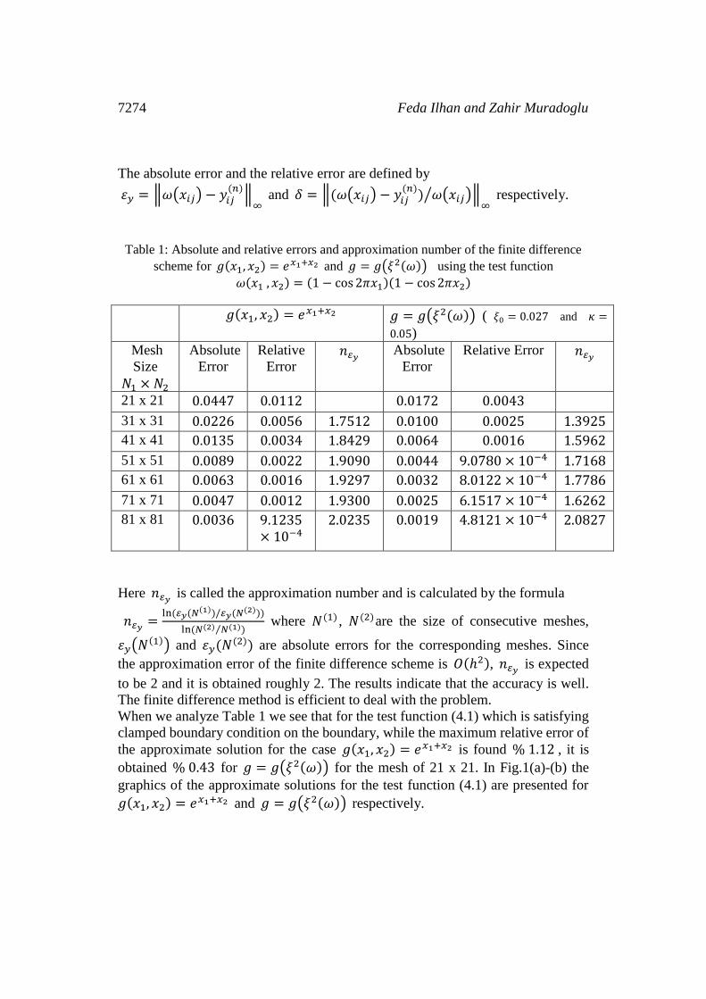
The absolute error and the relative error are defined by

휀𝑦 = ‖𝜔(𝑥𝑖𝑗) − 𝑦𝑖𝑗(𝑛)

‖∞

and 𝛿 = ‖(𝜔(𝑥𝑖𝑗) − 𝑦𝑖𝑗(𝑛)

) 𝜔(𝑥𝑖𝑗)⁄ ‖∞

respectively.

Table 1: Absolute and relative errors and approximation number of the finite difference

scheme for 𝑔(𝑥1, 𝑥2) = 𝑒𝑥1+𝑥2 and 𝑔 = 𝑔(𝜉2(𝜔)) using the test function

𝜔(𝑥1 , 𝑥2) = (1 − cos 2𝜋𝑥1)(1 − cos 2𝜋𝑥2)

𝑔(𝑥1, 𝑥2) = 𝑒𝑥1+𝑥2 𝑔 = 𝑔(𝜉2(𝜔)) ( 𝜉0 = 0.027 and 𝜅 =

0.05)

Mesh

Size

𝑁1 × 𝑁2

Absolute

Error

Relative

Error 𝑛𝜀𝑦

Absolute

Error

Relative Error 𝑛𝜀𝑦

21 x 21 0.0447 0.0112 0.0172 0.0043

31 x 31 0.0226 0.0056 1.7512 0.0100 0.0025 1.3925

41 x 41 0.0135 0.0034 1.8429 0.0064 0.0016 1.5962

51 x 51 0.0089 0.0022 1.9090 0.0044 9.0780 × 10−4 1.7168

61 x 61 0.0063 0.0016 1.9297 0.0032 8.0122 × 10−4 1.7786

71 x 71 0.0047 0.0012 1.9300 0.0025 6.1517 × 10−4 1.6262

81 x 81 0.0036 9.1235× 10−4

2.0235 0.0019 4.8121 × 10−4 2.0827

Here 𝑛𝜀𝑦 is called the approximation number and is calculated by the formula

𝑛𝜀𝑦=

ln (𝜀𝑦(𝑁(1))/𝜀𝑦(𝑁(2)))

ln (𝑁(2) 𝑁(1)⁄ ) where 𝑁(1) , 𝑁(2)are the size of consecutive meshes,

휀𝑦(𝑁(1)) and 휀𝑦(𝑁(2)) are absolute errors for the corresponding meshes. Since

the approximation error of the finite difference scheme is 𝑂(ℎ2), 𝑛𝜀𝑦 is expected

to be 2 and it is obtained roughly 2. The results indicate that the accuracy is well.

The finite difference method is efficient to deal with the problem.

When we analyze Table 1 we see that for the test function (4.1) which is satisfying

clamped boundary condition on the boundary, while the maximum relative error of

the approximate solution for the case 𝑔(𝑥1, 𝑥2) = 𝑒𝑥1+𝑥2 is found % 1.12 , it is

obtained % 0.43 for 𝑔 = 𝑔(𝜉2(𝜔)) for the mesh of 21 x 21. In Fig.1(a)-(b) the

graphics of the approximate solutions for the test function (4.1) are presented for

𝑔(𝑥1, 𝑥2) = 𝑒𝑥1+𝑥2 and 𝑔 = 𝑔(𝜉2(𝜔)) respectively.

Numerical solution of non-linear biharmonic equation 7275

Fig. 1: Approximate solution of the test function 𝜔(𝑥1 , 𝑥2) = (1 − cos 2𝜋𝑥1)(1 −

cos 2𝜋𝑥2) for 𝑔(𝑥1, 𝑥2) = 𝑒𝑥1+𝑥2 and 𝑔 = 𝑔(𝜉2(𝜔)) in the figures (a) and (b)

respectively

Similarly, when the absolute and relative errors which are obtained by using the test

function (4.2) are analyzed, for 𝑔(𝑥1, 𝑥2) = 𝑒𝑥1+𝑥2 the relative error of the

numerical solution is % 0.06 and it is obtained of % 0.26 for the nonlinear case.

That means the finite difference scheme that is obtained for finding the approximate

solution of the nonlinear problem is applicable. In addition, when the table given

above is examined further, we deduce that as the mesh size increases the absolute

and the relative errors decrease.

Next, real implementation problems which satisfy various boundary conditions are

discussed and the maximal deflections occurred on the surface of the bending plate

are compared. The geometrical and physical parameters given in Table 2 are used

for all examples considered below.

Table 2: The data used for the computational experiments.

Geometric properties

Side length of the plate 𝑙1 = 𝑙2 = 10 [𝑐𝑚]

Thickness of the plate ℎ = 0.3 [𝑐𝑚] Mesh size 𝑁1 × 𝑁2 = 25 × 25 Physical properties

Elastic parameters 𝐸 = 21000 𝑘𝑁𝑐𝑚−2 , 𝜈 = 0.5

𝜅 = 0.45, 𝜉02 = 2.1

Example 1: A load is applied at the central and four symmetric neighboring nodes

of the elasto-plastic plate which has the geometric and physical properties given in

Table 2. For different initial approaches iteration number for obtaining numerical

solution is derived. The results for clamped and simply supported boundary

conditions are given in Table 3.

00.2

0.40.6

0.81

0

0.5

10

1

2

3

4

G3

(a)

G1

00.2

0.40.6

0.81

0

0.5

10

1

2

3

4

5

6

7

G3

(b)

G1

7276 Feda Ilhan and Zahir Muradoglu

Table 3: Iteration number for different initial approaches 𝜔(0)(𝑥1, 𝑥2) where

‖𝜔(𝑘+1)(𝑥𝑖𝑗) − 𝜔(𝑘)(𝑥𝑖𝑗)‖∞

< 휀

휀

Clamped boundary condition

(𝑞 = 350[𝑘𝑁]) Simply supported boundary

condition (𝑞 = 290[𝑘𝑁])

0.01 0.001 0.0001 0.01 0.001 0.0001

𝜔(0) Iteration number Iteration number

𝑒𝑥1+𝑥2 15 19 24 17 20 26

𝑒𝑥12+𝑥2 20 25 30 23 26 31

𝑠𝑖𝑛𝜋𝑥1𝑠𝑖𝑛𝜋𝑥2 7 12 17 9 13 18

Example 2: It is assumed that a load 𝐹(𝑥) is applied at the central and four

symmetric neighbouring nodes of the elasto-plastic plate which has the geometric

and physical properties given in Table 2. The intensity of the applied load is 𝑞 =

320 [𝑘𝑁]. For the initial approach 𝜔(0)(𝑥1, 𝑥2) = 𝑒𝑥12+𝑥2 and with the accuracy

휀 = 0.001 the numerical solution of the nonlinear problem is obtained. For the

case which clamped boundary condition (2.2) is satisfied on the whole boundary,

the graph of the bending surface of the plate is given in Fig.2(a) and when the

simply supported boundary condition (2.3) is satisfied the bending surface graph of

the plate is given in Fig.2(b).

Fig. 2: (a) Numerical solution for the clamped boundary condition.(b) Numerical solution

for the simply supported boundary condition

When the clamped boundary condition is satisfied, the approximate solution of the

problem, corresponding to the given value of the load is reached after 𝑛 = 25

iterations, while the simply supported boundary condition is satisfied the

approximate solution is found for 𝑛 = 28 iterations. For clamped and simply

supported boundary conditions the maximal deflections occurred at the central

point of the elasto-plastic plate are obtained as 𝜔𝑚𝑎𝑥 = 2.4059 [𝑐𝑚] and 𝜔𝑚𝑎𝑥 =5.2986 [𝑐𝑚] respectively. The expected result that the deflection of the plate

02

46

810

0

5

10-3

-2

-1

0

1

G3

(a)Numerical Solution

G1

02

46

810

0

5

10-6

-4

-2

0

2

G3

(b)Numerical Solution

G1

Numerical solution of non-linear biharmonic equation 7277

which satisfy simply supported boundary condition is more than the deflection of

the plate satisfying clamped boundary condition is obtained.

Example 3: An elasto-plastic plate which has the geometric and physical

properties given in Table 2 are taken and for the increasing values of the intensity of

the load 𝑞𝑘 applied at the central point of the plate which has clamped and

simply supported boundary respectively. The maximal value of deflection and

𝜉2(𝜔𝑚𝑎𝑥) values corresponding to these deflections are observed (Table 4).

Table 4: Variation of maximal deflection 𝜔𝑚𝑎𝑥 and 𝜉2 for increasing values of intensity

of the load 𝑞𝑘 which is applied to the elasto-plastic plate satisfying clamped and simply

supported boundary condition

Clamped Boundary Condition Simply Supported Boundary Condition

k 𝑞𝑘 𝜔𝑚𝑎𝑥 [𝑐𝑚] 𝜉2(𝜔𝑚𝑎𝑥) 𝑞𝑘 𝜔𝑚𝑎𝑥 [𝑐𝑚] 𝜉2(𝜔𝑚𝑎𝑥)

1

2

3

4

5

260

290

317.4

320

350

1.9524

2.1777

2.3835

2.4059

2.6663

1.4183

1.7396

2.1019

2.2085

3.7081

200 230 260.2 290 320

3.1729 3.6488 4.1281 4.6495 5.2986

1.2319 1.6292 2.1050 3.9374 7.0831

From Table 4 one sees that for the plate satisfying clamped boundary condition the

load 𝑞3 = 317.4[𝑘𝑁] corresponds to the last elastic state since the effective value

of plate curvature is 𝜉2(𝜔𝑚𝑎𝑥) = 𝜉02 = 2.1. This means that for all 𝑞(𝑥) > 𝑞3

there will arise plastic deformations and for all 𝑞(𝑥) < 𝑞3 the deformations will be

elastic. Similarly, when the same applications are made for a plate satisfying simply

supported boundary condition, the load to be applied for the last elastic state is

260.2[𝑘𝑁] and 𝜉2(𝜔𝑚𝑎𝑥) = 2.1 = 𝜉02

.If the applied load is less than

260.2 [𝑘𝑁] elastic deformation occurs i.e. when the effect of the applied load is

removed the bending plate returns to the its initial shape. If the intensity of the

applied load 𝑞(𝑥) > 260.2[𝑘𝑁] then when the load is removed the trace of

deformation remains on the plate. Relation between the intensity of the loads and

maximal deflections for the plate satisfying clamped and simply supported

boundary conditions is given in Fig. 3(a). Additionally, for this implementation

problem it is observed that as the intensity of the applied load increase the

deflection of the bending plate increase.

7278 Feda Ilhan and Zahir Muradoglu

Fig. 3: (a) Relation between the intensity of the loads and maximal deflection for the plate

satisfying clamped and simply supported boundary conditions. (b)The relation between

deformation and thickness of the plate satisfying clamped boundary condition

Example 4: An elasto-plastic plate which has the geometric and physical

properties given in Table 2 is taken and loads of different intensities are applied at

the central and four symmetric neighbouring nodes of the plate. When the plate

thickness is changed the change in deformation is observed for the clamped

boundary condition (Table 5).

Table 5: Maximal deflections for different thickness

k h [cm] 𝜔𝑚𝑎𝑥 [𝑐𝑚] q=260 [kN] q=318 [kN] q=350 [kN]

1

2

3

4

5

6

7

8

0.26

0.28

0.30

0.32

0.34

0.36

0.38

0.40

3.1939

2.4046

1.9524

1.6087

1.3412

1.1299

0.9607

0.8237

4.2971

3.0972

2.3890

1.9676

1.6404

1.3819

1.1750

1.0074

5.0568

3.5630

2.6666

2.1656

1.8055

1.5210

1.2932

1.1088

When Table 5 is analyzed we see that, when thickness of the plate increases the

maximal deflection decreases whatever the force is (Fig. 3(b)).

Example 5: We take an elasto-plastic plate satisfying only the geometric

properties given in Table 2. This plate is assumed to be made of rigid and soft

materials respectively. For changing values of the strength hardening parameter

𝜅 , the maximal deflections on the surface of the bending plate for different

boundary conditions are obtained and results are given in Table 6 and for rigid and

soft materials respectively.

0.2 0.25 0.3 0.35 0.4 0.450

1

2

3

4

5

6

7

8

Plate Thickness [cm]

Defl

ect

ion

[cm

]

(b)Deflections for different thickness

0 2 4 6 8 10 12 14 16 180

100

200

300

400

500

600

700

Deflection

Loa

d

(a)Deflections produced by the loads of different intensities

simply supported boundary

clamped boundary

Numerical solution of non-linear biharmonic equation 7279

Table 6: Deflections 𝜔𝑚𝑎𝑥[𝑐𝑚] on the surface of elasto-plastic plate made of rigid and

soft material for different 𝜅 values

𝜅

𝐸 = 21000[𝑘𝑁𝑐𝑚−2]

𝜉02 = 2.1 𝑞 = [320 𝑘𝑁]

𝐸 = 11000[𝑘𝑁𝑐𝑚−2]

𝜉02 = 1.1 𝑞 = [130 𝑘𝑁]

Clamped Simply

Supported

Clamped Simply

Supported

0.45

0.35

0.15

2.4059

2.4046

2.4035

5.2986

5.1913

5.1053

1.8855

1.8752

1.8667

4.2069

4.0777

3.9721

From Table 6 we deduce that the smaller strength hardening parameter 𝜅 , the less

deflection on the surface of the plate. Because as 𝜅 decreases, the rigidity of the

material increases. Numerical examples indicate that the finite difference method

possesses no numerical difficulty in the analysis of the elasto-plastic problem of the

plate.

5 Conclusions

We obtained a numerical solution for the boundary value problem related to the

fourth order nonlinear PDE for a bending plate by using finite difference method

with various boundary conditions. The results given in the computational

experiments have interesting aspects from both mathematical and engineering

points of view. The presented numerical examples show the effectiveness of the

given approach.

References

[1] S. Timoshenko, A Course in the Theory of Elasticity, Naukova Dumka, Kiev,

1972.

[2] S. Lurie, V. Vasiliev, The Biharmonic Problem of the Theory of Elasticity,

Gordon and Breach Publishers, London, 1995.

[3] A. Hasanov, Variational approach to non-linear boundary value problems for

elasto-plastic incompressible bending plate, Int. J. Nonl. Mech., 42 (2007),

711-721. http://dx.doi.org/10.1016/j.ijnonlinmec.2007.02.011

[4] D. R. J Owen, E. Hinton, Finite Elements in Plasticity: Theory and Practice,

Pineridge Press, UK, 1980.

[5] H Armen Jr., A. Pifko, H.S. Levine, A Finite Element Method for the Plastic

Bending Analysis of Structure, Grumman Aircraft Engineering Corporation,

Bethpage, New York, 1998.

7280 Feda Ilhan and Zahir Muradoglu

[6] S. S. M. Auatt, V J. Karam, Analysis of elastoplastic Reissner's plates with

multi-layered approach by the boundary element method, Mecánica

Computacional, 21 (2002), 1317-1327.

[7] A. Moshaiov, W S. Vorus, Elasto-plastic plate bending analysis by a boundary

element method with initial plastic moments, Int J. Solids and Struct., 22 (1986),

1213-1229. http://dx.doi.org/10.1016/0020-7683(86)90077-6

[8] S.B.S. Abayakoon, M.D. Olson, D.L. Anderson, Large deflection

elastic-plastic analysis of plate structures by the finite strip method, Int. J. Numer.

Meth. Eng., 58 (1989), 331-358. http://dx.doi.org/10.1002/nme.1620280207

[9] H. Amoushahi, M. Azhari, Buckling of composite FRP structural plates using

the complex finite strip method, Compos. Struct., 90 (2009), 90-99.

http://dx.doi.org/10.1016/j.compstruct.2009.02.006

[10] J. Belinha, L.M.J.S. Dinis, Elasto-plastic analysis of plates by the element

free Galerkin method, Eng. Comput., 23 (2006), 525-551.

http://dx.doi.org/10.1108/02644400610671126

[11] P. Xia, S. Y. Long, K. X. Wei, An analysis for the elasto-plastic problem of

the moderately thick plate using the meshless local Petrov Galerkin method, Eng.

Ana. Boundary Elem., 35 (2011), 908-914.

http://dx.doi.org/10.1016/j.enganabound.2011.02.006

[12] L. M. Kachanov, Fundamentals of the Theory of Plasticity, North- Holland

Publishing Company, Amsterdam, London, 1971.

[13] K. Washizu, Variational Methods in Elasticity and Plasticity, 2nd ed.,

Pergamon, New York, 1981.

[14] S. P. Timoshenko, S. Woinowsky-Krieger, Theory of Plates and Shells, 2nd

ed., McGraw- Hill International Editions, 1959.

[15] A. Langenbach, Elastisch- plastische deformationen von platten, Z. Angew.

Math. Mech., 41 (1961), 126- 134. http://dx.doi.org/10.1002/zamm.19610410306

[16] A. Hasanov, A. Mamedov, An inverse problem related to the determination

of elasto-plastic properties of a plate, Inverse Problems, 10 (1994), 601- 615.

http://dx.doi.org/10.1088/0266-5611/10/3/007

[17] A. A. Samarskii, V. B. Andreev, Difference Methods for Elliptic Problems,

Nauka, Moscow, 1976, (in Russian).

Received: December 1, 2015; Published: December 16, 2015