HAL Id: hal-01289900https://hal-ensta-paris.archives-ouvertes.fr//hal-01289900

Submitted on 17 Mar 2016

HAL is a multi-disciplinary open accessarchive for the deposit and dissemination of sci-entific research documents, whether they are pub-lished or not. The documents may come fromteaching and research institutions in France orabroad, or from public or private research centers.

L’archive ouverte pluridisciplinaire HAL, estdestinée au dépôt et à la diffusion de documentsscientifiques de niveau recherche, publiés ou non,émanant des établissements d’enseignement et derecherche français ou étrangers, des laboratoirespublics ou privés.

On experimental sensitivity analysis of an axisymmetricturbulent wake

M Grandemange, M Gohlke, V Parezanović, Olivier Cadot

To cite this version:M Grandemange, M Gohlke, V Parezanović, Olivier Cadot. On experimental sensitivity analysis of anaxisymmetric turbulent wake. Physics of Fluids, American Institute of Physics, 2012, 24, pp.035106.hal-01289900

On experimental sensitivity analysis of an axisymmetric turbulent wake

M. Grandemange,1, 2 M. Gohlke,2 V. Parezanović,1 and O. Cadot1

1Unité de Mécanique, Ecole Nationale Supérieure de Techniques Avancées,

ParisTech, Chemin de la Hunière, 91761 Palaiseau Cedex, France2PSA Peugeot Citroën, Centre Technique de Velizy,

Route de Gisy, 78943 Vélizy-Villacoublay Cedex, France

The sensitivity to local disturbances of the turbulent wake over a 3D blunt body with an

axisymmetric detachment is investigated at Re = 2.1·104. The flow presents a favored m = 2

azimuthal symmetry set by two wings. The instantaneous wake is measured either above or

below the plane containing the wings but leads a statistical symmetric wake. Topology shifts

are random but occur mostly after a large number of global mode periods. The statistical

symmetry is highly sensitive to any asymmetric disturbance. As a consequence, depending

on its position a small control cylinder in the close wake fixes the wake to one asymmetric

topology affecting shedding activity and drag. The effect of an axisymmetric perturbation

(m = 0) on flow topology and dynamics is also studied ; it induces significant drag reductions

and global mode modifications when acting on mixing layers. Whatever the disturbance, the

sensitivity of the wake seems concentrated into the mixing layers and may depend more on

their local turbulent characteristics than on the inviscid dynamics of vorticity.

I. INTRODUCTION

New theoretical efforts have allowed to obtain the structural sensitivity of global mode wakes in

laminar regimes1–3. Over bidimensional geometries, this approach is able to recover qualitatively

the sensitivity obtained experimentally by Strykowski and Sceenivasan4. Recently, Meliga et al.5,6

performed similar studies in the wake of axisymmetric bodies ; zones of high sensitivity have been

found in the recirculating bubble, particularly around the separatrix. Although the theory is still

limited to basic flows and laminar regimes, this approach might provide a useful tool in the frame

work of control strategy since it predicts the placement of a disturbance to efficiently affect global

properties of the flow. For practical and industrial interests, the method should be extended to

large Reynolds number flows over complex geometries. So far, no theory is available in turbulent

regimes however, over cylinders, some qualitative similitudes persist between laminar theoretical

analyses and experiments at moderate Reynolds numbers7–9. The empirical results of Parezanović

and Cadot9 point out that the distrubance of the close wake leads to variations of global mode

2

A = ⟨a⟩ average value of a

Std(a) standard deviation of a

a∗ non-dimensional value of a

|a| modulus of a

cD drag coefficient

cp pressure coefficient

D diameter of the body base

dR diameter of the control ring

H = δ∗/θ boundary layer shape factor

Lb recirculation length

p0 inlet flow pressure

P (#A) probability of state #A

P (#A|#B) probability of state #A, given #B

Re = U0D/ν Reynolds number

St = fD/U0 Stouhal number

StS Strouhal number of the global mode

Stb characteristic Stouhal number of the recirculation

Tb characteristic time of the recirculation

u = ux.ex + uy.ey + uz.ez velocity

uij =√u2i + u2

j modulus of velocity in plane (ei,ej)

U0 inlet flow velocity

vE characteristic velocity of flow incorporation into the mixing layers

xC position x of the control cylinder

xR position x of the control ring

yC position y of the control cylinder

yα position y verifying Ux∗(x∗, y∗, z∗ = 0) = α

δ99 boundary layer thickness based on 99% of freestream velocity

δ∗ boundary layer displacement thickness

δM mixing layer thickness base on 10% and 90% of freestream velocity

Ωz mean vorticity in z direction

ρ density of the fluid

θ boundary layer momentum thickness

Table I: Nomenclature

frequency and base pressure. The associated physical mechanisms seem relied on the perturbation

ability to change the size of the formation region of the von-Kármán street vortices and to interact

3

with the shear layers.

Over axisymmetric bodies, the dynamic of the separated flow is more complicated than the

bidimensional von-Kármán street. Indeed, the wake undergoes several transitions associated to

different wake regimes as the Reynolds number increases10. At very low Reynolds numbers, the

flow is steady and axisymmetric. A first bifurcation is reported (for Re ≈ 210 over spheres) : a

steady azimuthal mode m = 1 appears. A lift force is generated and a pair of counter-rotating

vortices develops downstream moving the wake off streamwise axis so the flow loses its axisymmetry

but keeps a planar symmetry. A second bifurcation occurs at a higher Reynolds number (Re ≈ 277

over spheres) : the wake starts oscillating but preserves the same planar symmetry. Becoming

turbulent, the preference toward this azimuthal plane of symmetry vanishes and the flow becomes

statistically axisymmetric11. At moderate Reynolds numbers, the high frequency mixing layer

instabilities in the close wake degenerate into large scale vortex loops developing from the end

of the recirculation bubble ; the wake oscillates randomly10,12 and may get a helical structure

highly coherent in space13–15. This unsteady global mode (dominant mode m = 1) is reported at

0.1 < St < 0.2 depending on geometry and Reynolds number.

Previous experiments of passive and active control of the turbulent wake show connections between

parameters of the control set-up, drag and global mode intensity14,16–20. In particular, Berger et

al.14 proves that disk forced to oscillate near the helical mode frequency stabilizes this mode in

space and time at a coherence level close to 1. Weickgenannt et al.17 performed experiments

displacing a control disk in the recirculation bubble pointing out different flow regimes depending

on the disk position associated to important evolutions of drag and Strouhal number. However

this control set-up may be too intrusive to be considered as a local perturbation.

The present work explores the sensitivity of wake of a 3D blunt body with a fixed axisymmetric

flow separation at Re = 2.1 · 104. Experiments of passive control using reasonably small devices

are performed to disturb the flow with m = 0 and m = 1 perturbations ; to our knowledge, such

an approach has not been carried out over bodies of revolution so far. The impact of the control

device is reported through sensitivity maps of global mode frequency, pressure distribution on the

body and estimation of the drag.

The article is organized as follows. First, the natural flow is analysed ; it is proved that two

antisymmetric flows cohabit and generate a statistically symmetric natural flow. Then the

sensitivity to different local perturbations is investigated. Any m = 1 disturbance change the

statistical equilibrium of the mean flow moving it off axis. On the contrary, a m = 0 disturbance

preserve the mean flow symmetry but has significant impacts global mode frequency and drag. The

4

sensitivity of the flow seems concentrated in the close wake, particularly into the mixing layers.

Eventually, the effects of these disturbances on the wake orientation and global mode frequency

are discussed ; past tridimensional bodies, the turbulent characteristic of the wake might play a

greater role than the inviscid dynamics of vorticity.

II. EXPERIMENTAL SET-UP

The Eiffel type wind tunnel is an open loop air flow facility. The turbulent intensity is less than

0.3% and the homogeneity of the velocity over the 400 mm× 400 mm blowing section is 0.4%. The

wake is generated by a 3D symmetric blunt body ; its geometry is based on the "D" shape cylinder

used in the experiments of Parezanović and Cadot8. The body is made up by a cylinder of diameter

D = 50 mm and a half sphere forebody. The total length is L = 125 mm. The axisymmetric body

is supported by two NACA 0021 profiles fixing the azimuthal planes of symmetry (xOy) and (xOz)

(see Fig. 1). Most experiment are performed with the blunt body aligned to incoming flow, however

when specified a small pitching angle ϵ is set to add an antisymmetric disturbance.

The main flow velocity is U0 = 6.5 m.s−1 and the Reynolds number (Re = U0D/ν) is 2.1 · 104.

The velocities are defined as u = ux.ex + uy.ey + uz.ez ; uij =√

u2i + u2j is the amplitude of

velocity at the considered point in the plane (ei,ej). A and Std(a) are respectively average value

and standard deviation of any quantity a. The diameter D, density ρ, inlet velocity U0 and static

pressure p0 are used to obtain non-dimensional values marked with an asterisk.

The separated flow is first controlled by a 3 mm diameter cylinder oriented along z direction

and moved in the wake using a robot. xC and yC refer to the cylinder position (see Fig. 1(a)).

Except when located on the streamwise axis, the cylinder is considered a m = 1 disturbance.

The other control devices are flat rings with a length of 6 mm and a thickness of 1 mm mounted on

a 3 mm diameter rod (see Fig. 1(b)). xR represents the gap between the base of the body and the

ring center. The point R remains on the streamwise axis so the symmetry of the body is preserved

and the rings are associated to m = 0 perturbations. Nine ring diameters dR between 0.7 and 1.1D

are used to disturb the close wake.

A wake analysis is made from PIV and stereo PIV measurements respectively in planes z∗ = 0

and x∗ = 1.2. Statistics from 2000 instantaneous velocity field estimate the fluctuating velocity

energy. To get unsteady characteristics of the flow, a 1D hot wire probe mounted on a three-axis

robot records the velocity in the wake at a sampling frequency of 2 kHz. Power spectra are then

5

x

xx x

Figure 1: Experimental set-up of the body controlled by a 3 mm cylinder (a) and rings (b) ; O sets the

origin of the coordinate system ; pitching angle ϵ = 0 in most experiments.

calculated up to 1 kHz with a resolution of 0.5 Hz.

In addition, the pressure on the body is measured in the plane z∗ = 0. Thirteen taps are located

on the half sphere of the forebody every 15 ; the seven others give the pressure distribution on

the base, the space between base taps is 6 mm. Pressure measurements are performed at 1 Hz over

120 s; the sampling frequency of 1 Hz is limited by the acquisition device : the record is a mean

over at least 1 s to preserve precision.

The drag is estimated by integration of the interpolated pressure on the surface projected on x

direction ; pressure distributions in each region y∗ > 0 and y∗ < 0 are assumed axisymmetric :

CD =1

12ρπ

D2

4 V02

[ ∫∫bodyp ds

].ex

≈ 4

∫ 0.5

y∗=−0.5Cpnose(y

∗) · |y∗| dy∗

−4

∫ 0.5

y∗=−0.5Cpbase(y

∗) · |y∗| dy∗. (1)

For the uncontrolled flow, the so-evaluated drag is CD 0 = 0.261±0.002. Experimenting the method

presented by Weickgenannt et al.17 based on momentum deficiency in the far wake, a higher value

of 0.29 is measured, partially due to friction effects. When the control device is in the wake, its

contribution to the drag is neglected.

6

III. RESULTS

A. Natural flow

The boundary layer at the trailing edge is fully turbulent and depends on the azimuth due

to the presence of the wings in the plane y∗ = 0. The boundary layers at detachment in planes

y∗ = 0 and z∗ = 0 are presented on Figure 2(a). A separation is observed on the upper and lower

part of the the end of the forebody. The flow reattaches turbulent on the cylindrical part before

the massive separation at the trailing edge. This boundary layer history leads to the mean and

fluctuating velocity profiles in the plane z∗ = 0 (see empty and filled circles on Fig. 2(a)). The

energy of the fluctuations of velocity diminishes when y∗ increases and tends to the free flow level

of turbulence. This particularly high fluctuation level in the entire boundary layer is a result of

the forebody detachment.

In the plane y∗ = 0, the wake of the wings leads to a velocity deficiency and a turbulent boundary

layer at the trailing edge at y∗ ≈ 0 (see empty and filled squares on Fig. 2(a)). As the wake of the

wings is present at y∗ = 0, the fluctuations of velocity remains large even outside the boundary

layer. The characteristics obtained from these velocity profiles are presented in table II. The high

shape factor of the turbulent boundary layer is certainly due to the adverse pressure gradient along

the side of the body.

BL at y∗ = 0.5 and z∗ = 0 BL at y∗ = 0 and z∗ = 0.5

δ99 1.57 mm ±0.05 mm 1.82 mm ±0.05 mm

δ∗ 0.36 mm ±0.02 mm 0.40 mm ±0.02 mm

θ 0.18 mm ±0.02 mm 0.19 mm ±0.02 mm

H 2.0 ±0.3 2.1 ±0.3

Table II: Boundary layer characteristics at the trailing edge.

After detachment, the mixing layers grows from the trailing edge to the far wake. Figure 2(b)

displays the streamwise velocity profiles in plane z∗ = 0 at different positions x∗. The size of the

mixing layer is defined as δM (x) = y0.9(x) − y0.1(x) with yα(x) verifying Ux∗(x, yα(x)) = α. The

experiments of Champagne et al.21 report that plane turbulent mixing layers has a characteristic

growth rate constant dδM ∗/dx∗ ∼ 0.1. In parallel, the eddy viscosity model predicts that it expands

toward the low velocity domain22. The contours of Ux∗ = 0.1, 0.5 and 0.9 (positions of yα(x) for

7

Figure 2: (a) Mean and fluctuating velocity profiles respectively empty and filled markers at the trailing

edge in plane z∗ = 0 (blue ⃝) and y∗ = 0 (red ) ; the hot wire probe measures respectively Uxy and Uxz.

(b) Streamwise velocity profiles in the upper mixing layer from PIV in plane z∗ = 0 at different x∗ positions:

—, x∗ = 0.2 ; - -, x∗ = 0.4 ; ··, x∗ = 0.6 ;-·-, x∗ = 0.8. (c) Contours of streamwise velocity Ux∗ from PIV in

plane z∗ = 0: ··, 0.1 ; —, 0.5 ; - -, 0.9.

α = 0.1, 0.5 and 0.9) are plot on Figure 2(c). The growth of δM is approximatively linear between

x∗ = 0.1 and x∗ = 0.7 and dδM∗/dx∗ is measured respectively at 0.17 and 0.18 for the upper

and lower mixing layer. The expansion occurs toward the recirculation bubble where Ux∗ ∼ 0, the

contours Ux∗ = 0.9 being roughly parallel to the streamwise axis. This particularly high growth rate

in comparison to the results presented by of Champagne et al.21 may be due to the axisymmetry of

the wake but also to the oscillations induced by the presence of a global mode. Indeed, the power

spectrum analysis of hot wire probe signals at (x∗, y∗, z∗) = (4, 0.5, 0) reports a wake oscillation

at frequency fS = 25.8 Hz, i.e. StS = 0.199 (see Fig. 3). The two peaks at St ≈ 0.05 and 0.07

correspond to wind tunnel signature.

Figure 4(a) displays the streamlines of the time-averaged PIV measurements in the plane

8

Figure 3: Power spectrum analysis of hot wire probe signal at (x∗, y∗, z∗) = (4, 0.5, 0).

Figure 4: Streamlines of the time-average vector field in the plane z∗ = 0 ; colormap of the mean vorticity

Ωz (a) and fluctuating velocities (b) ; white cross, collar point.

Figure 5: Streamlines of the velocity field in the plane z∗ = 0 (a) and in the plane x∗ = 1.2 (b) for slightly

nose-up configuration, state #1 ; colormap of the fluctuating velocities ; white cross, collar point.

z∗ = 0. The natural wake is symmetric referring to the plane y∗ = 0 with two recirculation

structures and two collar points at x∗ = 0.95 and y∗ ≈ ±0.2 (see Fig. 4(b)). This topology is

consistent with the two pairs of counter-rotating vortex proposed by Delery23 ; the converging

streamlines at y∗ ≈ ±0.2 for x∗ > 1 are the signatures of these streamwise vortices in the symmetry

plane z∗ = 0, one pair at y∗ ≈ 0.2 and the other at y∗ ≈ −0.2. The vorticity concentrated in the

9

Figure 6: Flow computed from velocity field #1 in plane z∗ = 0 (see Fig. 5(a)) and the expected velocity

field for state #2.

boundary layer vanishes from the detachment to the end of the recirculating bubble. The vorticity

is only measured near the recirculation separatrix : the recirculation structures do not contain

vorticity. The maximum fluctuating energy is measured at y∗ ≈ ±0.4 and x∗ ≈ 0.8 (see Fig. 4(b)).

Theses fluctuations are partially associated to the development of the unsteady global mode. As

expected, it is equally present at the top and the bottom of the end of the recirculation bubble.

In agreement with remarks present in literature17,23, the symmetry of the wake is highly sensitive

to the set-up configuration. An ϵ incidence moves the whole wake up or down. Figures 5(a)–(b)

present the asymmetric wake topology for a slightly nose-up configuration. Measurements in

the plane x∗ = 1.2 show only one pair of counter-rotating vortices at y∗ ≈ −0.3 and z∗ ≈ ±0.2

just above a single zone of intense fluctuations. Therefore, as soon as the symmetry is lost, the

unsteady m = 1 mode develops mostly from the lower part of the wake. It is associated to the

formation of parallel hairpin shaped vortex loops at the end of the recirculation bubble10,24. When

the symmetry is preserved, these vortex loops must develop statistically from both sides of the

wake.

The observed balanced wake for ϵ = 0 (see Fig. 2(b)) is consistent with an average of two

asymmetric topologies (named #1 and #2), each of them being respectively close to the flow

presented on Figures 5(a)–(b) and its symmetric referring to the plane y∗ = 0. Indeed, averaging

the velocity field Uϵ for state #1 shown on Figure 5(a) with the expected flow for state #2,

an artificial velocity field can be computed: Ux(x∗, y∗) = 1

2(Uxϵ(x∗, y∗) + Uxϵ(x

∗,−y∗)) and

Uy(x∗, y∗) = 1

2(Uyϵ(x∗, y∗) − Uyϵ(x

∗,−y∗)). This artificial wake presented on Figure 6 has exactly

the same properties as the measured one over a lined-up body : two collar points associated to two

zones of intense fluctuations of velocity at y∗ ≈ ±0.4.

10

Two different wake positions are then expected for the flow over a lined-up configuration

i.e. ϵ = 0. When the wake follows the configuration #1, the upper recirculation structure is bigger

and closer to the base than the lower one. This asymmetry of the recirculation bubble leads to

an average diagonal recirculating flow and a non-uniform pressure distribution on the base ; the

base pressure gradient dCp/dy∗ is negative in state #1 (see Fig 7(a)). The slope of the linear fit

of the base pressure distribution gives the average pressure gradient and indicates whether the

instantaneous flow follows the state #1 or #2. Hence, each record of base pressure distribution

gives the dominant topology over the second of measurement.

The time evolution of the base pressure signal during 5 · 103 s is studied. The pressure gradient,

i.e. the dominant topology, is shown on Figure 7(b) over 1000 s . Two preferred positions are

visible at dCp/dy∗ ≈ ±0.1. This point is confirmed by the probability density function presented

on Figure 7(c). The two topologies #1 and #2 respectively associated to negative and positive

gradients (-0.7 and 0.9) are clearly visible. The presence of the minimum between these peaks

suggests that a sampling period of 1 s remains below the mean shift time estimated at 4.6 s,

i.e. more than 100 global mode periods. The standard deviation of the base pressure gradient is

0.084. This value is equivalent to the absolute values of pressure gradients associated to states

#1 and #2 presented on the histogram Figure 7(b). Such a high value is then an indicator of the

coexistence of the two wake topologies. Eventually, the spectrum analysis of this signal over the

5 · 103 s does not present any characteristic frequency : the process seems random.

The two asymmetric topologies are then discriminated against the sign of the base pressure

gradient. The probability of state #1 or #2 at a moment t (resp. named St = #1 and St =

#2) depends not only on geometrical parameters like incidence but also on the past events (see

Tab. III). P (St = #1) < P (St = #1 | St−1 = #1) < P (St = #1 | St−1 = St−2 = #1) (idem for

topology #2), P (#A|#B) referring to the conditional probability of #A, given #B. As a result,

a configuration is more likely to appear at t if it was already there the seconds before.

P (St = #1) =0.53 P (St = #2) = 0.47

P (St = #1 | St−1 = #1) = 0.79 P (St = #2 | St−1 = #2) = 0.77

P (St = #1 | St−1 = St−2 = #1 ) = 0.85 P (St = #2 | St−1 = St−2 = #2 ) = 0.80

Table III: Probabilities of states #1 and #2 depending on the previous states over lined-up uncontrolled

configuration (precision better than 0.02), P (#A|#B) is the conditional probability of #A, given #B

11

Figure 7: (a) Base pressure distribution of topology #1 characterized by the negative slope of the linear fit

(continuous line), the corresponding bubble velocity field from Figure 4(b) is presented. (b) Time evolution

of 1 s averaged base pressure gradient over 1000 s. (c) Probability density function of base pressure slope in

y direction (precision ±0.01).

B. 3 mm control cylinder in the wake

Figure 8: Effect of the position of the 3 mm control cylinder on dCp/dy∗ (a) and on Std(dcp/dy∗) (b) ;

contours of Ux∗ for the natural flow: ··, 0.1 ; —, 0.5 ; - -, 0.9.

The asymmetric wake observed for a slight pitching angle highlights that average topology is

sensitive to any tiny change in geometrical configuration. As a consequence the control cylinder

which can be seen as a m = 1 steady disturbance should as well have significant impacts on

the flow. The base pressure gradient (i.e. the dominant topology) obtained as a function of the

cylinder position is presented on Figure 8(a). As expected, this m = 1 perturbation is highly

12

Figure 9: (a) Effect of the position of the control cylinder yC∗ at xC

∗ = 0.5 on the power spectrum at

(x∗, y∗, z∗) = (4, 0.5, 0) ; positions of Ux∗ for the natural flow: ··, 0.1 ; —, 0.5 ; - -, 0.9. (b) Strouhal of the

global mode as a function of the cylinder position ; the grey areas correspond to the absence of peak in the

measured power spectrum ; contours of Ux∗ of the natural flow: ··, 0.1 ; —, 0.5 ; - -, 0.9.

Figure 10: Effect of the position of the control cylinder on drag ; contours of Ux∗ for the natural flow: ··,

0.1 ; —, 0.5 ; - -, 0.9.

efficient in selecting the state #1 or #2. When positioned at xC∗ = 0.2 and yC

∗ = −0.3, it forces

the topology #1 (see Fig. 11(a)) ; if moved further downstream at constant yC∗ = −0.3 then the

configuration #2 dominates. When yC∗ = 0, the average wake is balanced (see Fig. 11(b)). For

xC∗ < 0.5 and yC

∗ = 0, there are also positions of the control cylinder where no pressure gradient

is induced despite the asymmetry of the configuration. At these locations, the fluctuation levels

of base pressure gradient over the 120 measurements is close to the natural value (see Fig. 8(b)).

This points out that both topologies #1 and #2 are present in the wake, the shift characteristic

time being implicitly between 1 s and 60 s. Further downstream, for xC∗ > 1, the flow is less

influenced by the control cylinder : the effect of the disturbance is not important enough to really

13

Figure 11: Streamlines in the plane z∗ = 0 for the controlled case xC∗ = 0.2 and yC

∗ = −0.3 (a) and

xC∗ = 0.5 and yC

∗ = 0 (b) ; colormap of the fluctuating velocities ; white cross, collar point. (c) Base

pressure distribution: — (×), natural flow ; - - (⃝), xC∗ = 0.2 and yC

∗ = −0.3 (see Fig. 11(a)) ; ·· (),

xC∗ = 0.5 and yC

∗ = 0 (see Fig. 11(b)).

set an asymmetric base pressure gradient and the fluctuation levels get back to the values of the

uncontrolled case. On the contrary, wherever the cylinder induces high positive or negative base

pressure gradient, i.e. topology #1 or #2, fluctuation levels of base pressure gradient are much

lower than the natural value : the control cylinder tends to stabilize the wake in one asymmetric

state depending on its position. Eventually, the fluctuations of base pressure remain quite low when

placed in the middle of the recirculation bubble ; either the wake is stabilized in a topology with a

uniform base pressure distribution or the mean shift time is under the measurement frequency of

1 Hz.

The cohabitation of the two topologies is then altered by this m = 1 disturbance and the

dynamic of the global mode is equally affected. The spectrum analysis of the hot wire probe

signal at (x∗, y∗, z∗) = (4, 0.5, 0) is presented on Figure 9(a) as a function of the cylinder position

yC∗ for xC

∗ = 0.5. As the probe is at y∗ = 0.5, the power spectrum map is not symmetric

referring to yC∗ = 0. A higher level energy is measured on the entire power spectra when the flow

follows topology #2, i.e. yC∗ < 0 at xC

∗ = 0.5. Indeed, the fluctuations of velocity are mostly

14

concentrated at the upper part of the recirculation and are convected downstream to the hot wire

probe whereas the levels of fluctuations are low at the probe while the flow follows state #1.

Figure 9(b) report the global mode frequency at positions where a peak of energy is present in the

power spectrum. This map is particularly correlated to the map of absolute values of base pressure

gradient. The more the control cylinder induced an asymmetric topology, the higher the frequency

is. On the contrary, StS tends to be reduced where the control cylinder sets dCp/dy∗ ∼ 0. An

exception is observed when yC∗ ≈ 0 but the energy associated to the global mode activity is

spreading over a large band of frequency and StS is poorly defined. For theses positions, the total

energy of the fluctuations of velocity may be slightly lower compared to that of the natural flow

(compare Fig. 11(b) to Fig. 4(b)) but remains at the same order of magnitude. In addition, the

two collar points are still observed in the wake. This tends to indicate that the flow is not sta-

bilized but that the two states #1 and #2 may still be present with a shifting time smaller than 1 s.

In parallel to these different flow modifications, drag is estimated through the pressure

distribution on the body. Drag reductions are mostly observed for xC∗ ≈ 0.5 and yC

∗ ≈ 0 (see

Fig. 10). The optimal position leads to a 8% decrease in drag mostly associated to a recovery

of base pressure (see Fig. 11(c)) ; the forebody pressure distribution is found independent of the

cylinder position. When the cylinder induces dCp/dy∗ ≈ 0 for yC∗ = 0, there is almost no effect on

the drag. At these locations, the flow does not seem disturbed by the cylinder, the only difference

is that the global mode frequency is slightly reduced.

C. Rings acting on mixing layers

Figure 12: Effect of the position of the control rings on Std(dcp/dy∗) ; contours of Ux∗ from uncontrolled

flow are plot: ··, 0.1 ; —, 0.5 ; - -, 0.9.

15

Figure 13: (a) Effect of the ring diameter dR∗ at xR∗ = 0.5 on the power spectrum at (x∗, y∗, z∗) = (4, 0.5, 0)

(see Fig 3 for comparison to natural flow) ; positions of Ux∗ of the natural flow are plot: ··, 0.1 ; —, 0.5 ; - -,

0.9.. (b) Effect of the position xR∗ of the dR

∗ = 0.85 ring on the power spectrum at (x∗, y∗, z∗) = (4, 0.5, 0)

(see Fig. 3 for comparison to natural flow and Fig. 13(a) for legend). (c) Strouhal number of the global

mode as a function of the ring position ; the grey areas correspond to the absence of peak in the measured

power spectrum ; contours of Ux∗ for the natural flow: ··, 0.1 ; —, 0.5 ; - -, 0.9.

Figure 14: Effect of the position of the control ring on drag ; contours of Ux∗ from uncontrolled flow are

plot: ··, 0.1 ; —, 0.5 ; - -, 0.9.

The sensitivity of the flow to m = 0 disturbances is now studied placing the rings in mixing

layers. The contribution of the 3 mm support to the following results can be estimated through the

effect of the control cylinder analyzed in the previous section when yC∗ = 0. As the perturbations

introduced by the rings are symmetric, the base pressure gradient remains null but its fluctuation

levels are still an indicator of stability. These fluctuations as a function of the ring diameter and

position are presented on Figure 12. For xR∗ < 0.8 the fluctuations of base pressure gradient tend

16

Figure 15: (a) Streamlines in the plane z∗ = 0 for the controlled flow with the dR∗ = 0.85 diameter ring

at xR∗ = 0.3 ; colormap of the fluctuating velocities ; white cross, collar point. (b) Idem Figure 15(a) at

xR∗ = 0.6. (c) Idem Figure 15(a) at xR

∗ = 0.8. (d) Base pressure distribution: — (×), natural flow ; - -

(⃝), xR∗ = 0.3 and dR

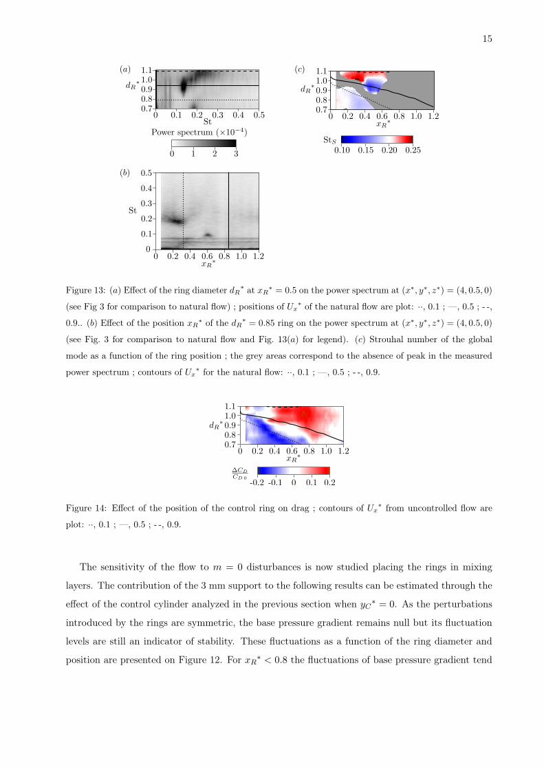
∗ = 0.85 (see Fig. 15(a)) ; ·· (), xR∗ = 0.6 and dR

∗ = 0.85 (see Fig. 15(b)) ; -·- (),

xR∗ = 0.8 and dR

∗ = 0.85 (see Fig. 15(c)).

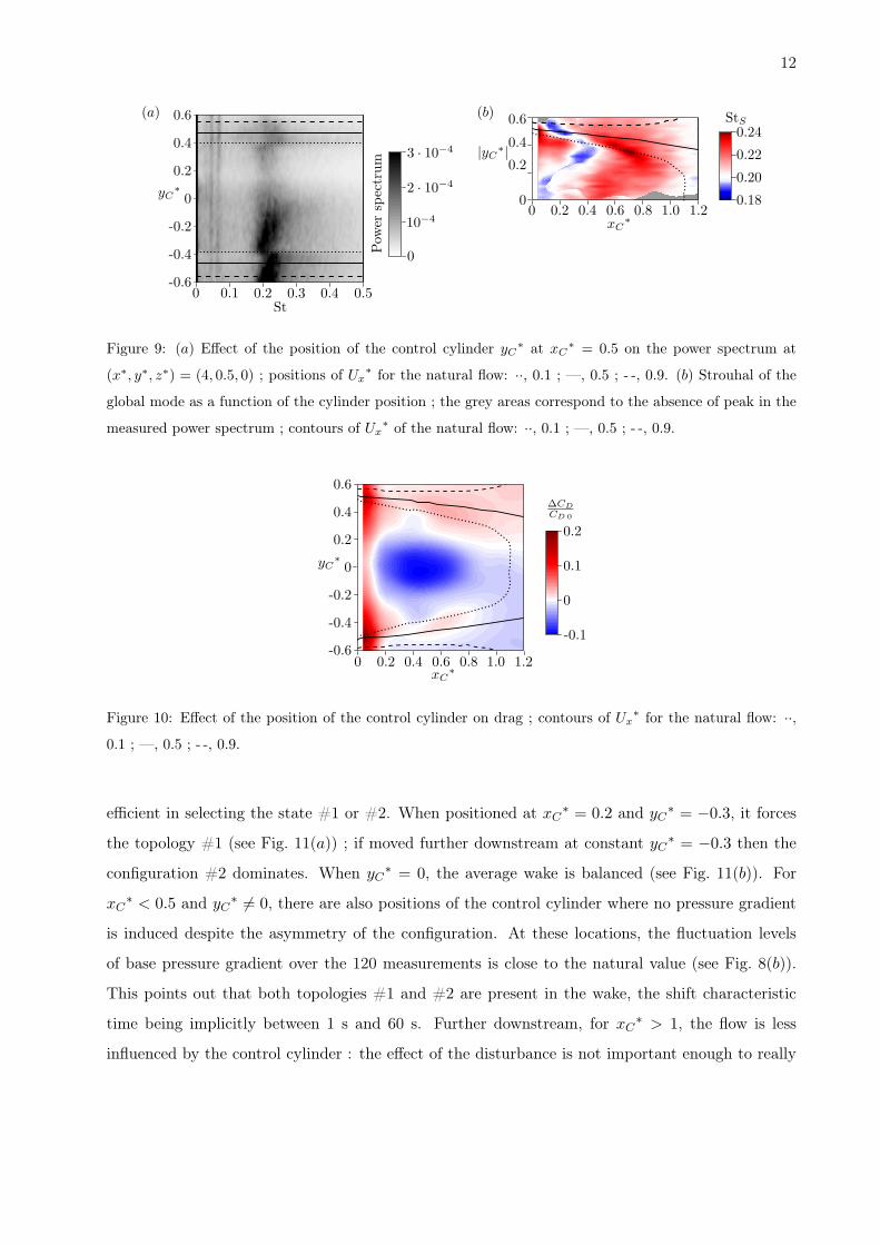
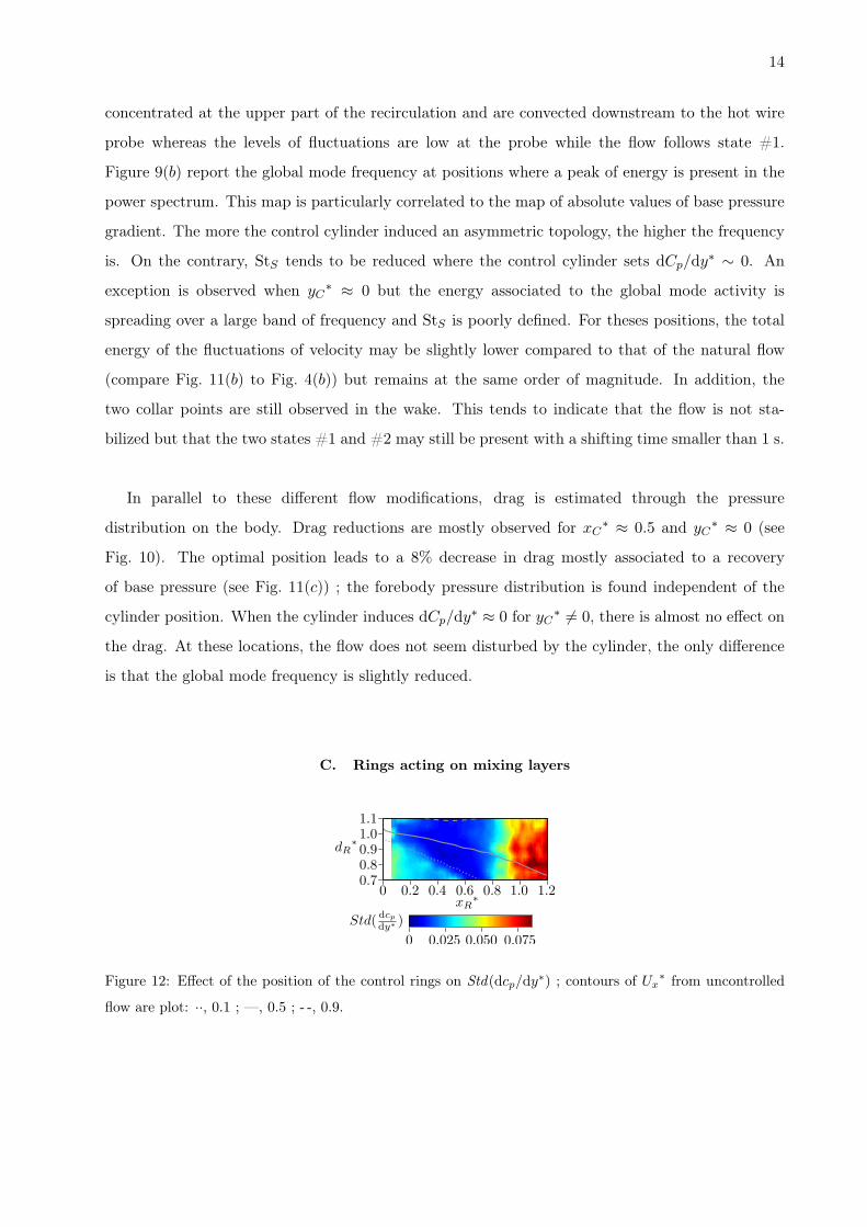
to be attenuated referring to the natural flow. In particular, the impact of the control ring on

Std(dcp/dy∗) follows the inner frontier of the mixing layer. As for the control cylinder, these low

values mean that either the wake is stabilized or the shift characteristic time is smaller than the

measurement sampling frequency. For xR∗ > 0.8, the fluctuations of base pressure gradient return

close to its natural values.

The modification of the global mode activity due to the presence the control rings is now

considered. Figures 13(a)–(c) present the power spectrum of the hot wire probe signal at

(x∗, y∗, z∗) = (4, 0.5, 0). For small ring diameters in the close wake (dR∗ < 0.85 and xR∗ < 0.2),

the disturbance is not in the mixing layer, the global mode frequency and amplitude are close to

the natural case. As the disturbance reaches the inner part of the mixing layer for xC∗ < 0.4,

the shedding frequency is decreased by approximately 15%. While the ring diameter increases,

the perturbation affects the middle of the mixing layer and the global mode is reported far less

energetic and then poorly defined (grey zones on Fig. 13(c)). Reaching the outer part of the mixing

layer, the global mode is measured again but at a higher frequency in comparison to the natural

17

value.

Further downstream for 0.4 < xC∗ < 0.6, a different scheme is observed (see Fig. 13(a)). As

measured for xC∗ < 0.4, the global mode frequency is reduced for small ring diameters and the

peak of energy in the spectra disappears increasing dR∗. In the middle of the mixing layer, a

new global mode regime is measured with a frequency of StS ≈ 0.1. Eventually, for dR∗ > 1, the

perturbation of the outer part of the mixing layer leads to an increase in global mode frequency.

For xR∗ > 0.6 whatever dR

∗ is, there is no more peak reported in the power spectra. The

attenuation of the global mode may be due to the presence of the 3 mm support. Indeed,

Figure 9(b) points out that the control cylinder prevent the global mode development when placed

on the streamwise axis for xC∗ > 0.7. Then, for these locations, the effect of the support may not

be negligible.

These evolutions in the dynamic of the flow result in drag reductions and increases. Figure 14

presents the estimation of the drag depending on the ring diameter and position. Alike the global

mode activity, the effect of the rings approximately follows the position of the mixing layer in

the natural flow. The optimal drag reductions are observed when the control device acts on the

inner part of the mixing layers. In opposition, drag is globally increased when the outer part of

the mixing layer is disturbed. An exception is present for xC∗ ≈ 0.2 where drag is also decreased

for the highest ring diameters. Thus, the drag evolutions do not directly correspond to the global

mode frequency map presented on Figure 13(c). Eventually, as observed with the control cylinder,

if xR∗ > 0.9 the effect is limited on drag indicating that the sensitivity of the flow is concentrated

particularly in the close wake mixing layers.

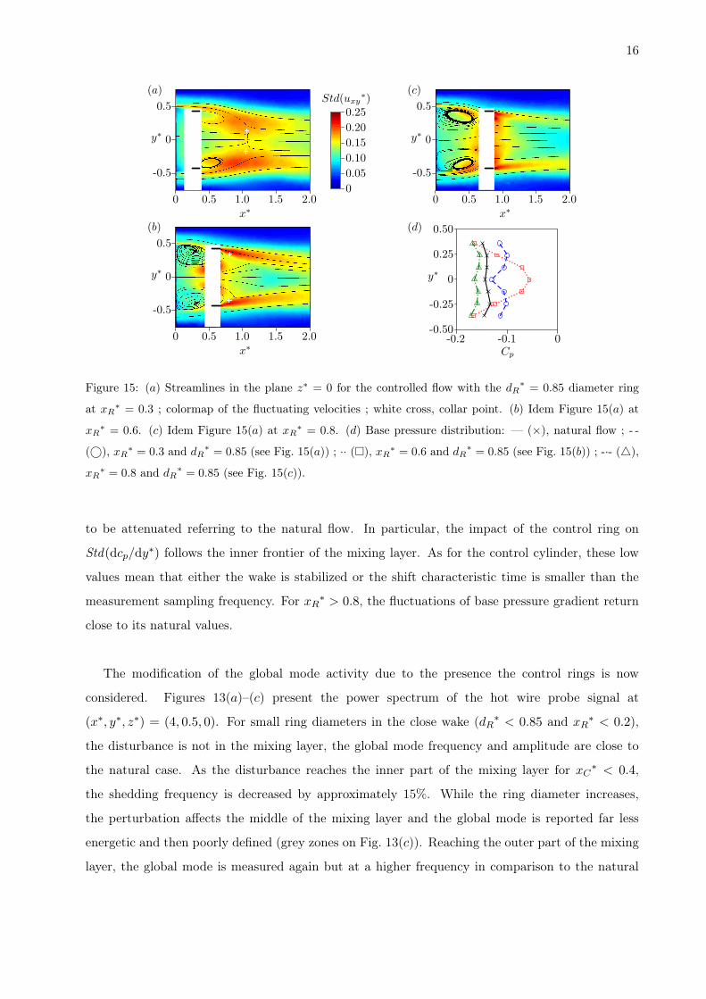
Different flow topologies correspond to these variations of drag and shedding frequency ; three

of them are presented on Figures 15(a)–(c) corresponding to xR∗ = 0.3, 0.6 and 0.8 for dR∗ = 0.85.

The associated spectra can be observed on Figure 13(b). At xR∗ = 0.3, a 14% decrease in CD is

measured. The associated velocity field is displayed on Figure 15(a). The recirculating structures

move downstream in comparison to the original flow (see Fig. 3 for comparison) and the bubble

length Lb is increased by 7.5%. The pressure recovery induced by the control device is distributed

on the entire base area (see Fig. 15(d)). This position of the ring also corresponds to a slight

reduction in global mode frequency is measured at St = 0.17 (see Fig. 13(b)).

Another topology is obtained with xR∗ = 0.6 and dR

∗ = 0.85. PIV measurements presented on

Figure 15(b) point out that the mixing layers reattach on the flat ring. The directions of the

18

streamlines around x∗ ≈ 0.8 indicate the presence of two stagnations points downstream the ring

but after the recirculation bubble ; thus they may not be associated to equivalents of states #1

and #2 but rather to the proper wake of the ring. The area where Ux∗ < 0 is strongly shortened

and the recirculation centers move near the body and the curvature of the recirculation separatrix

increases reducing peripheral base pressure. As shown on Figure 15(d), a compression occurs at the

center of the body due to an intensified recirculating flow in average. However this high pressure

at the base center is not sufficient to offset the loss of peripheral pressure. Indeed, the assumed

axisymmetry of the base pressure implies that the area associated to the pressure considered to

calculate drag is proportional to |y∗| (see (1)). The base pressure at y∗ ≈ 0 has then a smaller

impact on drag than at the periphery. The drag is measured equal to the uncontrolled case despite

this different topology corresponding to the low frequency global mode (StS ≈ 0.1).

A third topology associated to high drag case is presented on Figure 15(c). Alike for xR∗ = 0.6,

the flow reattaches on the rings and the recirculating structures are moved closer to the base of

the body inducing a shorter recirculation length. The drag is increased due to the loss of pressure

reported on the entire base : in opposition to the xR∗ = 0.6 there is not intense backward flow to

counter the loss peripheral base pressure. This position of the ring is associated to an absence of

global mode activity.

IV. DISCUSSION

A. On the global mode frequency

An unsteady global mode is usually observed in the flow past bluff bodies at moderate Reynolds

numbers : its frequency and energy depend on different parameters. Over cylinders, Gerrard25

presents a dynamic of the bubble in the wake considering the von-Kármán vortices. The flow

entrained from the bubble to the mixing layers is renewed by the flow injected at the end of

the recirculation through the velocity induced by the shear layers rollings. This model is highly

related to the vorticity dynamic following Biot & Savart law and leads to a dependence between the

characteristics of the shear layers and the global mode activity. The experiments of Parezanović

and Cadot9 recently confirm that the disturbance of the distance between the two shear layers or

their intensity impacts the global mode frequency. The presented results are in good agreement

with this Gerrard’s analysis : the Strouhal number of the global mode of the wake is governed by

19

the shear layer interaction.

The flow of over tridimensional geometries seems less influenced by the inviscid dynamics of the

vorticity in the wake. The global mode does not correspond to intense shedding and the refill of

the bubble presented by Gerrard is no more relevant. However, the dynamics of the flow can still

be analyzed considering that the turbulence characteristic of the wake is dominant. The growth of

the mixing layer is associated to the entrainment of fluid from both the bubble and the freestream

flow at a characteristic velocity vE following the relationship

vE dx ∼ U0 [δM (x+ dx)− δM (x)],

then

vE∗ ∼ dδM

∗

dx∗.

Estimating the bubble shape area and volume roughly at LbD and LbD2 with Lb the length in x

direction, a characteristic time of the dynamic of the bubble Tb can be defined. Tb corresponds to

the time needed to empty the volume of the bubble with a outflow speed vE over the interface.

LbDvE Tb ∼ LbD2,

Tb ∼D

U0vE∗ ∼ D

U0 · dδM ∗/dx∗.

The associated Strouhal number is

Stb ∼D

U0Tb∼ dδM

∗

dx∗. (2)

If the turbulent characteristic of the flow dominates its vorticity dynamic, then the global mode

frequency of the recirculation bubble may linearly depend on the growth of the mixing layers in

turbulent flows. The value of dδM ∗/dx∗ ≈ 0.17 is measured in our experiments for the natural flow

where the Strouhal of the shedding is measured at 0.199 so Stb ≈ α dδM∗/dx∗ with α ≈ 1. This

dependence is consistent with the observations of Achenbach24 on the Strouhal number of the wake

oscillation past a sphere. The frequency of this mode increases with the Reynolds number from

St = 0.12 at Re = 6 · 104 to St = 0.20 at Re = 3 · 105 just before the critical Reynolds number

is reached. At moderate Reynolds number, the mixing layer is laminar in the close wake and its

growth is slow ; this state is then associated to a low mode frequency. As the Reynolds number

20

increases, the mixing layer turns into turbulence before the end of the recirculation. The higher the

Reynolds number is, the sooner the transition occurs. This results in an increasing flow entrainment

into the mixing layers and an higher global mode frequency.

The effect of the control ring on the shedding frequency may be interpreted with this basic model

(see Fig. 13(c)). When the ring disturb the inner part of the mixing layer, the fluctuations of

velocity are reduced in the mixing layers. Their growth rate is then attenuated corresponding to an

increase in the recirculation length (see Fig. 14(a)). The associated shedding frequency is measured

slightly reduced. When the rings act on the outer mixing layer in the close wake, the mixing layer

may become more unstable and enhance fluid entrainment increasing the Strouhal number of the

mode.

Further downstream, a part of the mixing layer flow is oriented toward the streamwise axis and

the rings have their own wake. Thus, the dynamic of the flow changes drastically and the mode

frequency at St ≈ 0.1, when observed, cannot be compared to the natural value. Eventually, the

influence of the control cylinder on the global mode frequency is not discussed here. Indeed, m = 1

perturbations mostly impact the planar symmetry and the orientation of the wake, these effects are

analyzed in the following section.

B. On the azimuthal symmetry of the wake

It has been observed that any slight perturbation of the set-up leads to an asymmetric wake.

The work of Mittal et al.11 on shedding activity past spheres highlights that the Reynolds number

impacts the azimuthal position of the oscillating global mode m = 1. It appears that after the

unsteady bifurcation at Re ≈ 277 over a sphere, the global mode has a preferred azimuthal

orientation which may evolve at very low frequency. This effect disappears as Reynold number

increases and the wake gets statistically axisymmetric in turbulent flows. In our experiments even

at moderate Reynolds number, the wings prevent the statistical wake axisymmetry. The shedding

occurs mostly at the upper and lower part of the wake corresponding respectively to topology #2

and #1 but the mean flow keeps the top–bottom symmetry.

Any non-axisymmetric disturbance leads to a preferred azimuthal orientation for the antisymmetric

global mode. For example, as soon as the body has a small pitching angle, the shedding occurs

exclusively at the upper part of the wake or lower part depending on the sign of ϵ and the wake

loses this statistical symmetry. Therefore, if the disturbance has an azimuthal periodicity m = 1,

the shedding occurs in the same azimuthal plane, at the same side or the opposite one depending on

21

the position of the perturbation. This point was proved by Meliga et al.26 at low Reynolds numbers

through a theoretical analysis. Over blunt bodies of revolution, the forcing therm associated to

the presence of a m = 1 disturbance selects the plane of symmetry of the first bifurcation. The

different bifurcations observed in the wake of a disk degenerate into imperfect bifurcations and the

flow remains tridimensional, its orientation based on the azimuthal position of the perturbation.

When the disturbance has a higher azimuthal periodicity m ≥ 2, for example the two wings in

our experimental set-up associated to m = 2, the wake follows a statistical m flow topology. The

main coherent structure remains a m = 1 global mode shifting randomly between the m preferred

locations and generating a m statistical wake.

As a consequence, the experimental sensitivity analysis of the oscillating or helical mode m = 1 to

an antisymmetric perturbation can only be studied in the azimuthal plane of the disturbance. The

global mode follows any change of azimuthal position of the control leading to a mode sensitivity

independent of the azimuth.

The planar symmetry being set, the azimuthal phase of the wake is then 0 or π referring to the

position of the disturbance. The rate dδM∗/dx∗ may play a dominant role for the selection of the

phase, i.e. state #1 or #2. If one side of the axisymmetric mixing layer has a higher growth rate,

as previously seen, the development of δM toward the recirculation bubble is enhanced. Thus, the

curvature of the streamlines is increased27 and the whole wake is shifted to the opposite side where

the mixing layer remains thin. This concentration of vorticity leads to rolls-up and the development

of the vortex loops presented by Sakamoto & Haniu10.

This analysis coincides with the effect of small pitching angles ϵ and positions of the control cylinder.

Indeed over a nose-up configuration the upper boundary layer faces a higher adverse pressure

gradient than the lower one. This results in an increased height and a higher turbulence level at

the trailing edge. Therefore, the spread of the mixing layer is more intense on the upper side of the

recirculation bubble and the wake moves down, the vortex loops being generated from the lower

side of the bubble (see Fig. 5). In the same way, the control cylinder can enhance or reduce the

rate dδM∗/dx∗. In the close wake, when located in the inner part of the mixing layers the flow may

reattach on it, inhibiting the shear layers instability. Then the opposite mixing layer grows faster

and the wake moves in the direction of the disturbance (see Fig. 8(a)). Further downstream or in

the outer mixing layers, the control cylinder has its own wake generating important fluctuations

of the velocity fields. The disturbance intensifies the growth of the mixing layer and the wake

moves to the other side. Only cylinder positions in the mixing layers in plane z∗ = 0 are discussed

22

here ; when located inside the recirculation bubble, the cylinder get through the entire wake, the

disturbance is then much more complicated. The presented interpretation is no more pertinent.

V. CONCLUDING REMARKS

In conclusion, the natural flow over a body with an axisymmetric detachment is proved to be a

mean of asymmetric topologies. Due to the presence of two wings, i.e. m = 2 azimuthal periodicity

of the body, the wake is not axisymmetric but keep a statistical m = 2 symmetry. Instantaneous

wake follows a m = 1 azimuthal topology and is oriented either above or below the streamwise

axis (phase 0 or π), shifting randomly. The unsteady global mode then develops from on side of

the bubble depending on the orientation of the instantaneous wake.

A m = 1 disturbance, small pitching angle or control cylinder, sets one of the two asymmetric

topologies depending on its characteristics. This study highlights that the sensitivity of the flow

over a body of revolution to a non-axisymmetric local disturbance may only be observable in the

azimuthal plane of the perturbation. Any shift in the azimuthal position of the disturbance will be

followed by an equal shift of the azimuthal orientation of the global mode.

The use of control rings to generate a m = 0 disturbance has a strong influence on drag and wake.

As observed by Meliga et al.6, the effect follows the position of the mixing layers of the natural

flow. In particular, when placed in the inner part of the mixing layer, the rings may prevent the

development of the shear layer instability. It reduces the global mode frequency and moves the

wake structures downstream inducing significant drag reductions.

The mean flow symmetry as well as the global mode development are then highly sensitive

to any disturbance in the recirculation area, particularly when the mixing layers equilibrium or

characteristics are altered. The growth rate of the turbulent mixing layer seems to be a critical

factor for the flow dynamics, more than the inviscid dynamics induced by the vorticity.

Eventually, these results might be associated to the disturbance of the reminiscent global modes

observed in laminar regimes. The steady asymmetric wake reported after the first bifurcation

may concentrate the sensitivity to m ≥ 1 disturbances whereas the oscillating mode from the

second bifurcation (oriented along the steady asymmetric mode) seems more sensitive to m = 0

perturbations.

23

Acknowledgements

The authors wish to thank P. Meliga for fruitful scientific discussions.

1 D. Hill, A theoretical approach for analyzing the restabilization of wakes, NASA STI/Recon Technical

Report N 92 (1992) 29394.2 O. Marquet, D. Sipp, L. Jacquin, Sensitivity analysis and passive control of cylinder flow, Journal of

Fluid Mechanics 615 (-1) (2008) 221–252.3 P. Luchini, F. Giannetti, J. Pralits, Structural sensitivity of the finite-amplitude vortex shedding behind

a circular cylinder, in: IUTAM Symposium on Unsteady Separated Flows and their Control, Springer,

2009, pp. 151–160.4 P. Strykowski, K. Sreenivasan, On the formation and suppression of vortex ‘shedding’at low Reynolds

numbers, Journal of Fluid Mechanics 218 (1990) 71–107.5 P. Meliga, J. Chomaz, D. Sipp, Unsteadiness in the wake of disks and spheres: Instability, receptivity

and control using direct and adjoint global stability analyses, Journal of Fluids and Structures 25 (4)

(2009) 601–616.6 P. Meliga, D. Sipp, J. Chomaz, Open-loop control of compressible afterbody flows using adjoint methods,

Physics of Fluids 22 (2010) 054109.7 H. Sakamoto, H. Haniu, K. Tan, An optimum suppression of fluid forces by controlling a shear layer

separated from a square prism, ASME Transactions Journal of Fluids Engineering 113 (1991) 183–189.8 V. Parezanović, O. Cadot, The impact of a local perturbation on global properties of a turbulent wake,

Physics of Fluids 21 (2009) 071701.9 V. Parezanović, O. Cadot, Experimental sensitivity analysis of the global properties of a 2D turbulent

wake, Journal of Fluid Mechanics accepted for publication.10 H. Sakamoto, H. Haniu, A study on vortex shedding from spheres in a uniform flow, ASME, Transactions,

Journal of Fluids Engineering 112 (1990) 386–392.11 R. Mittal, J. Wilson, F. Najjar, Symmetry properties of the transitional sphere wake, AIAA journal

40 (3) (2002) 579–582.12 S. Taneda, Visual observations of the flow past a sphere at Reynolds numbers between 104 and 106,

Journal of Fluid Mechanics 85 (01) (1978) 187–192.13 H. Pao, T. Kao, Vortex structure in the wake of a sphere, Physics of Fluids 20 (1977) 187.14 E. Berger, D. Scholz, M. Schumm, Coherent vortex structures in thewake of a sphere and a circular disk

at rest and under forced vibrations, Journal of Fluids and Structures 4 (3) (1990) 231–257.15 G. Yun, D. Kim, H. Choi, Vortical structures behind a sphere at subcritical Reynolds numbers, Physics

of Fluids 18 (2006) 015102.

24

16 W. Mair, The effect of a rear-mounted disc on the drag of a blunt-based body of revolution(Drag of body

of revolution with blunt base substantially reduced by mounting disk behind body with smaller diameter

than body), Aeronautical Quarterly 16 (1965) 350–360.17 A. Weickgenannt, P. Monkewitz, Control of vortex shedding in an axisymmetric bluff body wake, Euro-

pean Journal of Mechanics-B/Fluids 19 (5) (2000) 789–812.18 A. Sevilla, C. Martinez-Bazan, Vortex shedding in high reynolds number axisymmetric bluff-body wakes:

Local linear instability and global bleed control, Physics of Fluids 16 (2004) 3460.19 H. Higuchi, Passive and Active Controls of Three-Dimensional Wake of Bluff-Body, JSME International

Journal Series B 48 (2) (2005) 322–327.20 J. Morrison, A. Qubain, Control of an axisymmetric turbulent wake by a pulsed jet, Advances in Tur-

bulence XII (2009) 225–228.21 F. Champagne, Y. Pao, I. Wygnanski, On the two-dimensional mixing region, Journal of Fluid Mechanics

74 (02) (1976) 209–250.22 H. Schlichting, K. Gersten, K. Gersten, Boundary-layer theory, Springer Verlag, 2000.23 J. Delery, Topologie des écoulements tridimensionnels décollés stationnaires : points singuliers, sépara-

trices et structures tourbillonnaires, Tech. rep., RT 121/7078 DAFE/N. ONERA (1999).24 E. Achenbach, Vortex shedding from spheres, Journal of Fluid Mechanics 62 (02) (1974) 209–221.25 J. Gerrard, The mechanics of the formation region of vortices behind bluff bodies, Journal of Fluid

Mechanics 25 (02) (1966) 401–413.26 P. Meliga, J. Chomaz, D. Sipp, Global mode interaction and pattern selection in the wake of a disk: a

weakly nonlinear expansion, Journal of Fluid Mechanics 633 (-1) (2009) 159–189.27 R. Simpson, Turbulent boundary-layer separation, Annual Review of Fluid Mechanics 21 (1) (1989)

205–232.