Online Appendix for:

International Evidence on Long-Run Money Demand

Luca Benati

University of Bern

Robert E. Lucas, Jr. University of Chicago

Juan-Pablo Nicolini

Federal Reserve Bank of Minneapolis and Universidad Di Tella

Warren Weber University of South Carolina, Bank of Canada,

and Federal Reserve Bank of Atlanta

Staff Report 588 June 2019

DOI: https://doi.org/10.21034/sr.588 Keywords: Long-run money demand; Cointegration JEL classification: E41, C32 An earlier version of this staff report circulated as Working Paper 738. The views expressed herein are those of the authors and not necessarily those of the Federal Reserve Bank of Minneapolis or the Federal Reserve System. __________________________________________________________________________________________

Federal Reserve Bank of Minneapolis • 90 Hennepin Avenue • Minneapolis, MN 55480-0291

https://www.minneapolisfed.org/research/

Online appendix for:International Evidence onLong-Run Money Demand

Luca BenatiUniversity of Bern∗

Robert E. Lucas, Jr.University of Chicago†

Juan-Pablo NicoliniFederal Reserve Bankof Minneapolis andUniversidad Di Tella‡

Warren WeberUniversity of South Carolina,

Bank of Canada, andFederal Reserve Bank of Atlanta§

A The Data

Here follows a detailed description of the dataset. Almost all of the data used in thispaper are from original sources. Specifically, they are from either (i) original hardcopy (books or, in the case of West Germany’s M1, scanned PDFs of the Bundesbank’sMonthly Reports, which are available from the Bundesbank’s website), in which casewe have entered the data manually into Excel; or (ii) central banks’ or nationalstatistical agencies’ websites (these data are typically available in either Excel orsimple text format). The few exceptions are discussed below. In those cases, we werenot able to find the data we were looking for in original documents, and thereforewe took them from either the International Monetary Fund’s International FinancialStatistics (henceforth, IMF and IFS, respectively) or the World Bank.

∗Department of Economics, University of Bern, Schanzeneckstrasse 1, CH-3001, Bern, Switzer-land. Email: luca.benati@vwi.unibe.ch

†Department of Economics, University of Chicago, 1126 East 59th Street, Chicago, Illinois 60637,United States. Email: relucas@uchicago.edu

‡Federal Reserve Bank of Minneapolis, 90 Hennepin Avenue, Minneapolis, MN 55401, UnitedStates. Email: juanpa@minneapolisfed.org

§ Email: wew@webereconomics.com

1

A.1 Argentina

All of the series are from the Banco Central de la República Argentina (Argentina’scentral bank, henceforth, Banco Central). Specifically, a series for M1, available forthe period 1900-2014, is from Banco Central ’s Table 7.1.4 (“Agregados Monetarios”).A series for a short-term nominal interest rate, available for the period 1821-2018, isfrom Banco Central’s Table 7.1.4 (“Tasas activas”). Interestingly, among all of thecountries we consider in this paper, Argentina is the only one that directly providesan estimate of (the inverse of) the velocity of circulation of monetary aggregates.Specifically, Banco Central’s Table 7.1.4 provides the ratios between either M1 andM3 and nominal GDP (“M1 % PBI” and “M3 % PBI,” respectively; “PBI” is theSpanish acronym for GDP). Based on the ratio between M1 and GDP, and the seriesfor M1, we then reconstructed a nominal GDP series.

A.2 Australia

An annual M1 series for the period 1900-2017 has been constructed in the followingway. A series for the period 1900-1973 has been kindly provided by Cathie Close ofthe Reserve Bank of Australia (henceforth, RBA). A monthly seasonally unadjustedseries, available since 1975, is from the RBA’s website (“M1, $ billion, RBA, 42216”;the series’ acronym is DMAM1N), and we converted it to the annual frequency bytaking annual averages (since for the year 1975 the series is available from February,the average for that year has been computed for the period February-December).The missing observation for 1974 has been interpolated as in Bernanke, Gertler,and Watson (1997), using as an interpolator series the IMF’s IFS series labeled as“Money,” which, over the overlapping periods, closely comoves with both M1 series.A series for a “short rate,” available for the period 1941-1989, is from Table 79 ofHomer and Sylla (2005). A 90-day nominal interest rate for bank accepted bills andnegotiable certificates of deposit is from the RBA’s website (“90-day BABs/NCDs,Bank Accepted Bills/Negotiable Certificates of Deposit-90 days, Monthly, Original,Per cent, AFMA, 42156, FIRMMBAB90”). It is available since 1969. A series fornominal GDP, available since 1960, is from the Australian Bureau of Statistics (“Grossdomestic product: Current prices; A2304617J; $ Millions”). An alternative seriesfor nominal GDP, available for the period 1870-2012, is from the website of theGlobal Price and Income History Group at the University of California at Davis, at:http://gpih.ucdavis.edu/.

A.3 Austria

A monthly seasonally unadjusted M1 series, available since January 1970, is fromthe European Central Bank. The series has been converted to the annual frequencyby taking simple annual averages. An annual series for the discount rate of the

2

Oesterreichische Nationalbank (Austria’s central bank), available for the period 1957-1998, is from the IMF ’s IFS. An annual series for nominal GDP is from StatisticsAustria since 1995, and from the IMF ’s IFS before then. Over the overlappingperiods, the two nominal GDP series are nearly identical, which justifies their linking.

A.4 Bahrain

An annual series for M1, available since 1965, is from the website of the Financial Sta-bility Directorate of the Central Bank of Bahrain. An annual series for “Interest Rateson BD Deposits & Loans,” available since 1976, is from the central bank’s StatisticalBulletin, available at: https://www.cbb.gov.bh/page-p-statistical_bulletin.htm. Anannual series for nominal GDP is from the website GCC-Stat, a statistical database forPersian Gulf countries (at: http://dp.gccstat.org/en/DataAnalysis?215Jv283P0CFmaBBdivhQ)since 2008. Before that, it is from the World Bank.

A.5 Barbados

An annual series for nominal GDP in million Barbados dollars, available since 1975, isfrom Tables I7A and I7B of the Barbados Statistical Service. An annual series for M1in million Barbados dollars, available since 1973, is from Table C1 from the CentralBank of Barbados. An annual series for the 3-month time deposits rate starting in1961 has been computed as the average of the two series “3 month Time Deposits- Lower FIDR_TD3L” and “3 month Time Deposits - Upper FIDR_TD3U,” fromthe Central Bank of Barbados.

A.6 Belgium

An annual M1 series (“Stock monétaire (milliards de francs)”), available for the period1920-1990, is from the Séries rétrospectives, Statistiques 1920-1990 from Banque Na-tionale de Belgique’s (Belgium’s central bank, henceforthBNB), Statistiques EconomiquesBelges, 1980-1990. For the period 1991-1998, M1 data are from the BNB’s BulletinStatistique. An annual series for nominal GDP (“Value Added at Market Prices inCurrent Prices, billion of francs”), available for the years 1920-1939 and 1946-1990,is from Smits, Woltjer, and Ma (2009). An annual series for the BNB’s discount rateavailable for the period 1920-1990 is from the Séries rétrospectives, Statistiques 1920-1990 from the BNB’s Statistiques Economiques Belges 1980-1990. For the period1991-1998, the discount rate is from several issues of the BNB’s Annual Report.

A.7 Belize

Annual series for M1 and for Belize’s Treasury bill rate, both available since 1977,are from the Central Bank of Belize. An annual series for nominal GDP, available

3

since 1970, is from the Penn World Tables Mark 7.0 until 2001, and from the CentralBank of Belize after that. Over the overlapping periods, the two nominal GDP seriesare near-identical, which justifies their linking.

A.8 Bolivia

Series for nominal GDP, M1, and a short-term nominal interest rate, all availablefor the period 1980-2013, are from the Unidad de Analisis de Politicas Sociales yEconomicas (Bolivia’s national statistical agency, known as UDAPE for short).

A.9 Brazil

Series for nominal GDP, M1, and GDP deflator inflation, all available for the pe-riod 1901-2000, are from IBGE’s (the Brazilian Institute of Geography and Sta-tistics) Estatisticas do Seculo XX (Statistics of the XX Century). The URL ishttp://seculoxx.ibge.gov.br/economicas. A series for nominal GDP for the period2000-2017 is also from IBGE. A series for M1 for the period 2000-2017 is from theBanco Central do Brasil (Brazil’s central bank, henceforth Banco Central). A seriesfor a short-term nominal interest rate for the period 1974-2012 is from the BancoCentral. Two series for a nominal government bond yield (for periods 1901-1913 and1929-1959) and the Banco Central ’s discount rate (for period 1948-1989) are bothfrom Homer and Sylla (2005)’s Table 81, pages 629-631.

A.10 Canada

An annual series for nominal GDP, available since 1870, has been constructed bylinking the Urquhart series (available from Statistics Canada (henceforth, SC ), whichis Canada’s national statistical agency), for the period 1870-1924; series 0380-0515,v96392559 (1.1) from SC, for the period 1925-1980; and series 0384-0038, v62787311(1.2.38) from SC, for the period 1981-2013. A short-term interest rate for the period1871-1907 (specifically, the “Montreal call loan rate”) is from Furlong (2001). Aseries for the o¢cial discount rate, available since 1926, has been constructed asfollows. Since 1934, when the Bank of Canada (Canada’s central bank) was created,it is simply the o¢cial bank rate (“Taux O¢ciel d’Escompte”) from the Bank ofCanada’s website. Before that, we use the Advance Rate, which had been set bythe Treasury Department for the discounting of bills, from Table 6.1 of Shearer andClark (1984).1 As for the latter period, we use a series for the 3-month Treasury billrate, which has been constructed by linking the series from the Historical Statistics

1To be precise, Shearer and Clark (1984) do not provide the actual time series for the AdvanceRate, but rather the dates at which the rate had been changed (starting from August 22, 1914),together with the new value of the rate prevailing starting from that date. Based on this information,we constructed a daily series for the rate starting on January 1, 1915, via a straightforward MATLABprogram, and we then converted the series to the annual frequency by taking annual averages.

4

of Canada, available for the period 1934-1935, to the series “Treasury Bill Auction -Average Yields - 3 Month, Per cent / en pourcentage” from the Bank of Canada. Amonthly series for M1 starting in January 1872 is from Metcalf, Redish, and Shearer(1996). This series is available until December 1952. After that, we link it via splicingto the series labeled as “Currency and demand deposits, M1 (x 1,000,000), v37213”from SC until November 1981. Finally, from December 1981 until December 2006,we use the series from SC labeled as “M1 (net) (currency outside banks, charteredbank demand deposits, adjustments to M1 (continuity adjustments and inter-bankdemand deposits) (x 1,000,000), v37200.” An important point to stress is that overthe overlapping periods, the three series are nearly-identical (up to a scale factor),which justifies their linking. For the period after December 2006, however, we werenot able to find an M1 series that could be reliably linked to the one we use forthe period December 1981-December 2006 (over the last several decades, Canada’smonetary aggregates have undergone a number of redefinitions, which complicatesthe task of constructing consistent long-run series for either of them). As a result,for the most recent period we have decided to use another series that we consider inisolation (that is, without linking it to any other M1 aggregate). The series is “M1B(gross) (currency outside banks, chartered bank chequable deposits, less inter-bankchequable deposits) (x 1,000,000), v41552787,” which is available since January 1967from SC. Finally, we convert all monthly series to the annual frequency by takingsimple annual averages.

A.11 Chile

Annual series for nominal GDP, the GDP deflator, and M1 are from Braun-Llona etal. (1998) for the period 1940-1995. As for the period 1996-2012, they are from theBanco Central de Chile, Chile’s central bank (specifically, nominal GDP and the GDPdeflator are from the Banco Central ’s Anuarios de Cuentas Nacionales, whereas M1is from Banco Central ’s Base Monetaria y Agregados Monetarios Privados). A short-term nominal interest rate (“1-day interbank interest rate, financial system average(annual percentage)”) from Banco Central is available for the period 1940-1995. Inorder to extend our analysis to the present as much as possible, we therefore alsoconsider, as an alternative measure of the opportunity cost of money, GDP deflatorinflation.

A.12 Colombia

Data for Colombia have been kindly provided by David Perez Reyna. Annual seriesfor nominal GDP and a short-term nominal interest rate for the period 1905-2003are from Junguito and RincÃsn (2007). As for the period 2004-2012, they are fromColombia’s Ministerio de Hacienda y Credito Publico. An annual series for M1 forthe period 1905-2012 is from the Banco de la Republica, Colombia’s central bank.

5

A.13 Ecuador

All of the data for Ecuador are from the website of Banco Central del Ecuador (hence-forth, BCE), Ecuador’s central bank. Most of them are from “85 Años, 1927-2012:Series Estadísticas Históricas,” a special publication celebrating BCE ’s 85th anniver-sary. Specifically, a series for annual CPI inflation (“Variación Anual del Indice Pon-derado de Precios al Cunsumidor por Ciudades y por Categorias de Divisiones deConcumo, Nacional”), available for the period 1940-2011, is from Chapter 4 of “85Años.” An annual series for a nominal interest rate has been constructed by linking theseries “Tasas, Máxima Convencional, En porcentajes,” available for the period 1948-1999; “Tasas de Interés Referenciales Nominales en Dólares, Máxima Convencional,”available for the period 2000-2007; and “Tasas de Interés Referenciales Efectivas enDólares, Máxima Convencional,” available for the period 2007-2011. All of them arefrom from Chapter 1 of “85 Años.” An annual series for nominal M1 in US dollars hasbeen constructed by linking the M1 aggregate (“Oferta Monetaria M1, En millones dedólares al final del período”), available for the period 2000-2011, which is expressedin US dollars, and the M1 aggregate (“Medio Circulante (M1), Saldos en millones desucres”), available for the period 1927-1999, which is expressed in Ecuador’s nationalcurrency, the sucre (both series are from Chapter 1 of “85 Años”). The latter M1aggregate has been converted in US dollars based on the series for the sucre/dollarnominal exchange rate found in Chapter 2 of “85 Años,” which is available for theperiod 1947-1999. Specifically, the exchange rate series (sucre per dollar) has beencomputed as the average between the “Compra” (i.e., buy) and the “Venta” (i.e., sell)series. An annual series for nominal GDP in U.S. dollars (“Producto interno bruto(PIB), Miles de dólares”), available for the period 1965-2011, is from Chapter 4 of“85 Años”. An important point to stress is that since we are working with M1 veloc-ity–defined as the ratio between nominal GDP and nominal M1–the specific unitin which the two series are expressed (US dollars, or Ecuadorian sucres) is irrelevant.

A.14 Finland

Long-run monthly data for M1 for the period January 1866-December 1985 have beengenerously provided by Tarmo Haavisto. The data come from his Ph.D. dissertation(see Haavisto (1992)) and have been converted to the annual frequency by takingsimple annual averages. A series for Finland’s monetary policy rate (labeled as the“Base rate”), available since January 1867, is from Suomen Pankki Finlands Bank(Finland’s central bank, henceforth, Suomen Pankki).2 Finally, an annual series for

2To be precise, Suomen Pankki does not provide the actual time series for the base rate, butrather the dates at which the rate had been changed (starting from January 1, 1867), togetherwith the new value of the base rate prevailing starting from that date. Based on this information,we constructed a daily series for the base rate starting on January 1, 1867, via a straightforwardMATLAB program, and we then converted the series to the annual frequency by taking annualaverages.

6

nominal GDP, available since 1860, is from Finland’s Historical Statistics, whichare available from the web page of Statistics Finland (Finland’s national statisticalagency). (To be precise, from the homepage of Statistics Finland, look at Home >Statistics > National Accounts > Annual national accounts > Tables.) Specifically,the nominal GDP series is B1GMHT (“Gross domestic product at current prices,1860-1960, million. mk”).

A.15 France

Annual series for nominal GDP, nominal M1, and the short rate are all from SaintMarc(1983). Specifically, the series for nominal GDP is the Toutain Index from AnnexeI: Revenu national, Produit Interieur Brut, pages 99-100 of Saint Marc (1983), andit is available for the period 1815-1913. The series for M1 is from the table “Vitesse-Revenu, Vy, et taux de liquidite, TL,”pages 74-75 of Saint Marc (1983), and it isavailable for the period 1807-1913. The series for the short rate is from Section7, “Evaluation des taux de l’interet,” pages 93-96, of Saint Marc (1983), and it isavailable for the period 1807-1913. In our analysis, however, we focus on the period1851-1913 because for the entire period 1820-1851, the short rate had been fixed at4%.

A.16 Guatemala

All of the data are from the Banco de Guatemala’s website. A series for nominalGDP is available for the period 1950-2017. A series for M1 (“M1 Medio Circulante-Millones de quetzales”) is available for the period 1980-2018. A series for a nominalshort rate (“Interest rate, Domestic currency, borrowing (passive)”) is available forthe period 1980-2018.

A.17 Hong Kong

An annual series for nominal GDP for the period 1961-2017 is from the Hong KongMonetary Authority’s (henceforth, HKMA) website (it is labeled as “Nominal GDP,HK$ million”). The series is from Table031 (“GDP and its main expenditure compo-nents at current market prices”). An annual series for M1 for the period 1985-2017is from the HKMA’s website (the series is labeled as “M1, Total, HK$ million”).An annual series for a short-term interest rate for the period 1982-2018 is from theHKMA’s website. The series is labeled as “Overnight rate, Table 6.3: Hong KongInterbank O§ered Rates”).

A.18 Israel

Series for nominal and real GDP, available since 1950, are from Israel’s Central Bu-reau of Statistics (henceforth, CBS ; special thanks to Svetlana Amuchvari of the CBS

7

for help with the data). Specifically, starting from 1995, the data are from Table 17 ofthe National Accounts. For the period 1950-1994, they are from the CBS ’s StatisticalAbstract of Israel (see columns D and J of Table 6.1, “National Income and Expen-diture: Resources and Uses of Resources”). The GDP deflator has been computed asthe ratio between the two series. An annual CPI inflation series (“Change in Level ofPrice Indices, Percentages, Annual, average”), available since 1971, is from the CBSwebsite (specifically, the series is from Table 13.1 of Statistical Abstract of Israel).For the period 1966-1975, the series for M1 is from Table 4.6, page 120, of Barkaiand Liviatan (2007). For the period since April 1981, a monthly M1 series is fromthe Bank of Israel ’s website (special thanks to Aviel Shpitalnik of the Bank of Israelfor help with the data). The series is M1.M (“M1 = Money supply, Monthly (M),NIS, million, Current prices”), and it has been converted to the annual frequency bytaking annual averages. A short-term interest rate for the period 1966-1974 is the“Nominal rate of return on MAKAM (3-month bills)” from Table 4.9, page 129, ofBarkai and Liviatan (2007). Since 1989 it is the Bank of Israel ’s “Actual e§ectiverate of interest,”from the Bank of Israel ’s website. For the period 1983-1988, we usethe “Discount Rate” from the IMF’s IFS. Over the overlapping periods (i.e., since1989), the Bank of Israel ’s actual e§ective rate of interest and the discount rate fromthe IMF are virtually identical, which justifies their linking.

A.19 Italy

Series for nominal GDP at current market prices, real GDP in chained 2005 euros, andthe implied GDP deflator, all available for the period 1861-2010, are from the sheet“Tab_03’ in the Excel spreadsheet ‘Data_Na150-1.1.xls,”which is available at theBanca d’Italia’s website at http://www.bancaditalia.it/statistiche/tematiche/stat-storiche/index.html. The spreadsheet contains the estimates of the Italian NationalAccounts’ aggregates, which are extensively discussed in Ba¢gi (2011). A series forM1, available for the period 1861-1991, is from the Data Appendix, pp. 49-52, ofFratianni and Spinelli (1997). Series for M1 and M2, available for the period 1948-1998, are from the table “Componenti della moneta dal 1948 al 1998” of BancadItalia(2013). In our analysis we use the M1 series from Fratianni and Spinelli (1997) forthe gold standard period, and the one from Banca d’Italia for the post-WWII period(over the overlapping periods, however, the two series are very similar, so in prac-tice this choice does not entail material implications). Short- and long-term interestrates for the period 1861-1996 are from Muscatelli and Spinelli (2000). A series forthe “Tasso U¢ciale di Sconto”–that is, Banca d’Italia’s o¢cial discount rate–isfrom the tables “Tassi d’interesse delle principali operazioni della banca centrale”and “Variazione dei tassi u¢ciali della Banca d’Italia, 1936-2003” of BancadItalia(2013).

8

A.20 Japan

Sources for Japanese data are as follows. A monthly series for the Bank of Japan’s(henceforth, BoJ ) discount rate, available since January 1883, is from the BoJ ’slong-run historical statistics, which are available at its website (the series is labeledas “BJ’MADR1M: The Basic Discount Rate and Basic Loan Rate”). Annual seriesfor nominal GNP and M1 for the period 1885-1940 are from Table 48 of Tamaki(1995). As for the period since 1955, data for nominal GDP and M1 are as fol-lows. Series for nominal GDP are from the Economic and Social Research Insti-tute (henceforth, ESRI ), Cabinet O¢ce, Government of Japan. (The key URLs arehttp://www.stat.go.jp/english/data/chouki/03.htm and

http://www.stat.go.jp/english/data/nenkan/1431-03.htm.) An important pointto stress here is the following. For the period before 1970, ESRI only provides tablesfor gross domestic expenditure, rather than gross domestic product. However, overthe overlapping periods (that is, 1970-1998), the relevant series coming from Table3-1 (“Gross Domestic Expenditure (At Current Prices, At Constant Prices, Defla-tors) - 68SNA, Benchmark year = 1990 (C.Y.1955—1998, F.Y.1955—1998), Value inbillions of yen”) and Table 3-3b (“3-3-b Gross Domestic Product Classified by Eco-nomic Activities (Medium Industry Group), (At Current Prices, At Constant Prices,Deflators) - 68SNA, Benchmark year = 1990 (1970—1998), Value in billions of yen”)are either numerically identical (in the case of nominal series) or numerically iden-tical up to a scale factor (in the case of real series and their deflators). This meansthat–as should be expected based on simple economic logic–the series that in Table3-1 is labeled as “Gross Domestic Expenditure” (Column Y in the Excel spreadsheet03-01.xls) is, in fact, nominal gross domestic product. As for M1, a monthly seriesfor the period January 1955-December 2018 was constructed by linking, via splicing,the following three series from the BoJ ’s website: MA’MAMS1EN01 (“(discontin-ued)_M1/Amounts Outstanding at End of Period/(Reference) Money Stock (Basedon excluding Foreign Banks in Japan, etc., through March 1999)”); MA’MAMS3EN01(“(discontinued)_M1/Amounts Outstanding at End of Period /(Reference) MoneyStock (fromApril 1998 toMarch 2008)”); andMA’MAM1NEM3M1MO (“M1/AmountsOutstanding at End of Period/Money Stock”). An important point to stress is that,over the overlapping periods, the series are essentially identical (up to a scale factor),which justifies their linking. Finally, the resulting monthly M1 series was convertedto the annual frequency by taking annual averages.

A.21 Mexico

A monthly interest rate series, available since January 1978, is from the Banco deMexico’s “Indicadores de tasas de interes de Valores Publicos” (Banco de Mexico,henceforth BdM, is Mexico’s central bank). It has been converted to the annual fre-quency by taking annual averages. Two annual interest rates series (“Interest Rate(%) Commercial loans” and “Interest Rate (%), O¢cial discount rate,”respectively)

9

are from Table 83, pages 639-640, of Homer and Sylla (2005). The first series isavailable for the periods 1942-1963 and 1978-1989. The second is available for theperiod 1936-1978. An annual series M1 for the period 1925-2000 is from the InstitutoNacional de Estadistica y Geografia (Mexico’s national statistical agency, henceforthINEGI ), “Estadisticas Historicas de Mexico, 2014,”and for the period 1985-2014 theyare from the BdM ’s website. The series from the BdM are available at the monthlyfrequency, and we converted them to the annual frequency by taking annual averages.Annual series for nominal GDP are from INEGI, “Estadisticas Historicas de Mexico2014”for the period 1925-1970; from the IMF’s IFS for the period 1970-1988; fromBdM for the period 1988-2004; and from INEGI for the period since 2004. The fourseries have been linked via splicing. An annual CPI inflation series available since1949 is from the IMF’s IFS (“Mexico, Consumer Prices, All items, Percent Changeover Corresponding Period of Previous Year”).

A.22 Morocco

A monthly seasonally unadjusted series for M1, available since January 1985, is fromthe website of Bank Al-Maghrib (the central bank of Morocco, henceforth, BAM ).The annual series has been computed by taking simple annual averages of the originalmonthly data. An annual series for nominal GDP, available since 1980, is from the“Comptes Nationaux” (National Accounts) from the website of the High Commissionfor Planning of Morocco. A series for the minimum rate applied to notebook accounts,available since January 1983, is from the website of BAM. BAM sets this interest ratetwo times a year, on January 1 and on July 1. The table at the central bank’s websitereports the values for the interest rate which have been set every January 1, and everyJuly 1, starting from 1983. From this information we computed the annual averagerates by taking a simple average within the year.

A.23 Netherlands

A series for the discount rate of De Nederlandsche Bank (the Dutch central bank,henceforth, DNB) for the period 1900-1992 is from Table 65 of Homer and Sylla(2005) until 1989 and from DNB ’s website after that. Series for nominal and real netnational income (NNI) and for the NNI deflator for the period 1900-1992 are fromTable 1, pages 94-95, of Boeschoten (1992). A series for M1, available since 1864, hasbeen constructed by linking the series from deJong (1967) and one from DNB.

A.24 New Zealand

A series for M1, available since 1934, is from the website of the Reserve Bank ofNew Zealand (henceforth, RBNZ ). A series for nominal GDP in million of Australiandollars is from Statistics New Zealand (New Zealand’s statistical agency). A series

10

for a short-term nominal interest rate starting in 1934 has been constructed in thefollowing way. Homer and Sylla’s (2005) Table 79 contains a series for the RBNZ ’so¢cial discount rate for the period 1934-1989. Since 1999, the RBNZ has been using,as its monetary policy rate, the “O¢cial Cash Rate,”which is available from theRBNZ ’s website. Since these two short-term rates have been used by the RBNZ asits o¢cial monetary policy rate for the periods 1934-1989 and 1999 to the present,respectively, they are in fact conceptually the same and can therefore be linked.For the period in between (1990-1998), for which no o¢cial monetary policy rate isavailable, we have used the “Overnight Interbank Cash Rate” from the RBNZ. Therationale for doing so is that since 1999, this rate has been very close to the O¢cialCash Rate, which justifies the linking of the two series.

A.25 Norway

A series for M1, available since 1919, is from the Historical Statistics of Norges Bank(Norway’s central bank), which are available at its website. Specifically, all histori-cal statistics for Norway’s monetary aggregates are from Klovland (2004). Series fornominal GDP and the GDP deflator, and for real GDP, real private consumptionexpenditures, and real gross investments (in millions of 2005 NOKs, i.e., kronas), allavailable since 1830, are from Norges Bank ’s Historical Statistics (for all series, theperiod 1940-1945 is missing). As for the short-term nominal interest rate, ideally wewould have liked to use Norges Bank ’s discount rate. The problem is that, althoughthe discount rate is available (from Norges Bank ’s website) since 1819, it has missingobservations for the period 1987-1990. As a result, we have resorted to using theAverage Deposit Rate (again, from Norges Bank ’s website), which is available since1822, has no missing observations, and over the period that is analyzed herein hasbeen quite close to the discount rate.

A.26 Paraguay

Annual series for CPI inflation (“Índice de Precios al Consumidor, ÁreaMetropolitanade Asunción, Indice General”), available for the period 1951-2015, and for nominalM1 in thousands of guaranies, available since 1962, are both from the website ofBanco Central del Paraguay (Paraguay’s central bank, henceforth BCP). An annualseries for nominal GDP in thousands of guaranies, available since 1960, is from theInternational Monetary Fund ’s International Financial Statistics.

A.27 Peru

All of the data for Peru are from the website of the Banco Central de Reserva delPerú, Peru’s central bank. An annual series for nominal GDP in million of nuevossoles is available since 1950. An annual series for inflation is available since 1901.

11

An annual series for nominal M1 in million of nuevos soles, available since 1959,has been constructed as the sum of currency in circulation (“Billetes y Monedas enCirculación”) and deposits (“Depósitos a la Vista del Sistema Bancario en MonedaNacional”).

A.28 Portugal

An annual series for M1 for the period 1854-1998 is from Table 5 of Mata and Valerio(2011). Annual series for real and nominal GDP for the period 1868-2008 are fromTable 4 of Mata and Valerio (2011). A series for the o¢cial discount rate of the Bancode Portugal (the Portuguese central bank), available for the period 1930-1989, is fromTable 74 of Homer and Sylla (2005).

A.29 South Africa

All of the data for South Africa are from the website of its central bank, the SouthAfrican Reserve Bank (SARB). Specifically, a series for the “Bank rate” (“Lowestrediscount rate at SARB”; code is KBP1401M) is available since 1923. A series forM1 (“Monetary aggregates / Money supply: M1, R millions”; code is KBP1371J) isavailable since 1967. A series for nominal GDP (“Gross domestic product at marketprices, R millions”; code is KBP6006J) is available since 1946.

A.30 South Korea

A series for M1 (“M1, Narrow Money, Average, Billion Won”) is available since 1970from the website of theCentral Bank of Korea (henceforth, BOK ), at: http://ecos.bok.or.kr.The series is from Table 1.1. (“Money & Banking (Monetary Aggregates, Deposits,Loans & Discounts etc.”). A series for nominal GDP (“Gross domestic product, cur-rent prices, Billion Won”) is available since 1953, again from the BOK’s website.A series for the central bank’s discount rate (“Republic of Korea, Interest Rates,Discount Rate, Percent per Annum”) is available since 1948 from the IMF’s IFS.

A.31 Spain

An annual series for M1 for the period 1865-1998 is from Cuadro 9.16 “AgregadosMonetarios, 1865-1998” of Barciela-LÃspez, Carreras, and Tafunell (2005), pp. 697-699 (the series is labeled as “M1, datos a fin de ano, en millones de pesetas”; the years1936-1940 are missing). An annual series for nominal GDP for the period 1850-2000is from Cuadro 17.7 of Barciela-LÃspez, Carreras, and Tafunell (2005), pp. 1338-1340 (the series is labeled as “El PIB a precios corrientes, 1850-2000, millones depesetas”; PIB is the Spanish acronym of GDP). An annual series for the “Descuentocomercial” of the Banco de Espana (Spain’s central bank, henceforth, BdE) is from

12

Cuadro 9.17 of Barciela-LÃspez, Carreras, and Tafunell (2005), pp. 699-701. Theseries is available for the periods 1874-1914, 1920-1935, and 1942-1985. An annualseries for the o¢cial discount rate of the BdE, available for the period 1930-1989, isfrom Table 74, pp. 541-542, of Homer and Sylla (2005). A monthly series for thethree-month Treasury bill rate available since March 1988 (“Tipo de interese hasta3 meses. Conjunto del mercado. Op. simples al contado. Letras del Tesoro.”), isfrom the BdE ’s website, and it has been converted to the annual frequency by takingannual averages (the data for 1988 have been ignored, since the series starts in Marchof that year).

A.32 Switzerland

Annual series for M1 (based on the 1995 definition) and the o¢cial discount rate of theSwiss National Bank (Switzerland’s central bank, henceforth SNB), all available atleast since 1929, are from the SNB ’s website. An annual series for nominal GDP avail-able for the period 1948-2005 is from the website of the project Economic History ofSwitzerland during the 20th century–see at http://www.fsw.uzh.ch/histstat/main.php.(Q.16b Gross domestic product (expenditure approach) in real 1990 prices and nom-inal, 1948-2005 in Million Swiss Francs).

A.33 Taiwan

All of the data are from the Central Bank of the Republic of China (Taiwan), thatis, Taiwan’s central bank (henceforth CBRCT ). An annual series for nominal GDP(“GDP by expenditures at current prices”) is available since 1951. An annual se-ries for the CBRCT ’s discount rate is available since 1962. Two annual series forM1 (“M1A (End of Period), M1A = Currency in circulation(currency held by thepublic)+Checking accounts and passbook deposits of enterprises, individuals andnon-profit organizations held in banks and community financial institutions” and“M1B (End of Period), M1B = M1A + Passbook savings deposits of Individuals andnon-profit organizations in banks and community financial institutions”) are bothavailable since 1962. In order to be sure that the series we use in this paper doesnot include components that go beyond a transaction purpose, we used the first one,M1A.

A.34 Thailand

An annual series for GDP at current prices in billions of baht, available for the pe-riod 1946-2005, is from Mitchell (2007). Since 1990 this series has been linked to thenominal GDP series from the Macro Economic Indicators of the Bank of Thailand(Thailand’s central bank, henceforth BoT ). Over the overlapping periods, the twoseries are very close, which justifies their linking. An annual M1 series in billions

13

of baht, available since 1970, has been constructed by taking, for each year, the De-cember observation from the series “Money supply (M1)” from Table 5 of the BoT ’smonetary aggregates for the period up to 2005. Since then, we have taken the De-cember observation from the monthly M1 series from the BoT ’s Macro EconomicIndicators. The reason for taking, for each year, the December observation, ratherthan computing the annual average, is that for the period 1970-1980 the Decemberfigure is the only one available for each year. An annual series for the 1-year maxi-mum interest rate on fixed deposits, available since 1979, is from the BoT ’s MacroEconomic Indicators.

A.35 Turkey

A monthly series for M1, available since January 1964, is from the website of Turkey’scentral bank, Turkiye Cumhuriyet Merkez Bankasi (henceforth, TCMB). The serieswe use has been constructed by taking simple annual averages of the original monthlydata. A series for the central bank’s discount rate is fromHomer and Sylla’s (2005) Ta-ble 74, pages 541-542, until 1990. After that, it is from TCMB. Specifically, TCMB ’swebsite reports the dates in which the discount rate was changed, together with thenew values taken by the discount rate at each date. Based on this information, foreach year since 1990 we have calculated the number of days in the year for which eachvalue of the discount rate has been in e§ect, and based on this we have computed, forevery year, a simple weighted average of the individual daily values of the discountrate. A series for the gross domestic product in current prices, available since 1967,is from the website of Turkey’s statistical o¢ce, TurkStat.

A.36 United Kingdom

All U.K. data are from version 3.1 of the dataset “A millennium of macroeconomicdata,” which is available from the Bank of England ’s website at:

http://www.bankofengland.co.uk/statistics/research-datasets. The first versionof the dataset (which was called “Three centuries of macroeconomic data”) was dis-cussed in detail in Hills and Dimsdale (2010). Specifically, series for M1, availablesince 1922; the Bank of England ’s monetary policy rate (known as the “Bank Rate”),available since 1694; and nominal GDP (“Nominal UK GDP at market prices”), avail-able since 1700, are, respectively, from columns A.24, A.31, and A.9 of the sheet “A1.Headline series.”

A.37 United States

The series for the 3-month Treasury bill rate; nominal GDP; both the “standard” M1aggregate and the “New M1” one; and Money Market Deposits Accounts (MMDAs),are all from Lucas and Nicolini (2015) All series have been updated to 2017 based

14

on either series’ updated original data sources. The original source for the 3-monthTreasury bill rate is the Economic Report of the President (henceforth, ERP), and theones for nominal GDP are Kuznets and Kendrick’s Table Ca184-191 before 1929, andTable 1.1.5 of the National Income and Product Accounts (henceforth, NIPA) afterthat. A series for Money Market Mutual Funds (MMMFs) starting in 1974 is from theFederal Reserve (the FRED II acronym is MMMFFAA027N, “Money market mutualfunds, Total financial assets, Billions of dollars”). An annual series for nominal GDPat current prices is from O¢cer and Williamson (2015).

A.37.1 Adjusting for the share of currency held by foreigners

As documented, for example, by Judson (2017), over the last several decades, thefraction of US currency held by foreigners has significantly increased, and it stood, atthe end of 2016, at around 50%-60% of total currency, depending on the methodologythat was used to estimate it. Since the demand for M1, which is being investigatedin the present work, is a demand on the part of US nationals, this raises the issueof how to adjust US currency in order to purge it of the fraction held by foreigners.This could be done in several ways, none of them ideal. One possibility would be,following Judson (2017), to estimate a model for the demand of Canadian currencyas a function of Canadian nominal GDP and interest rates, and then to apply theestimated coe¢cients to U. nominal GDP and interest rates in order to back out apredicted level of US currency demanded by US nationals. As extensively discussedin Judson (2017), the rationale for doing this is that–most likely as a consequenceof the similarity between the U.S. and Canadian economies–up until about 1990the ratios between currency and nominal GDP in the two countries had tended toclosely comove. Only since then has the demand for US currency on the part ofnon-US nationals skyrocketed, thus causing the traditional relationship between thedemands for U.S. and Canadian currency, as fractions of their respective GDPs, togo o§ kilter. For our own purposes, this approach su§ers from the limitation that,by definition, it produces a “fundamental,” predicted value for the demand for UScurrency on the part of US nationals which does not reflect idiosyncratic, transitoryfactors that are not captured by either nominal GDP or the short rate. Because ofthis, we have adopted an alternative approach in which we estimate the fraction ofUS currency held by foreigners as the simple di§erence between the ratios betweencurrency and nominal GDP in the United States and Canada. One problem with thisapproach is that since, during the early years of the Great Depression, Canada didnot experience banking collapses of a magnitude comparable to the United States,the “flight to currency” there was much more muted. As a result, our approachmechanically interprets the increase in the demand for US currency as a fraction ofGDP between the crash of 1929 and the inauguration of F.D. Roosevelt’s presidencyas an increase in demand on the part of foreigners. Our counterargument to this isthat the spike in the demand for currency, although sizable, was very short-lived,

15

as it only pertained to four years, from 1930 to 1933. As a result, since this onlypertains to currency–which, in 1929, was just 14.6% of overall M1–it is reasonableto assume that the impact of this on our estimates should be negligible.

A.38 Venezuela

Annual data for nominal GDP (“Producto Interno Bruto, Millones de Bolívares aPrecios Corrientes”), M1 (“Circulante, (M1), I.1, Circulante, Liquidez Monetaria yLiquidez Ampliada, Saldos al final de cada período en millones de bolívares”), and ashort-term rate (“Tasas de Interes Activas Anuales Nominales Promedio, Ponderadasde los Bancos Comerciales y Universales, Porcentajes”) are from the Banco Centralde Venezuela (Venezuela’s central bank). GDP is available since 1957, and M1 isavailable since 1940. The interest rate is available for the period 1962-1999. An alter-native monthly interest series, available since July 1997 (“Tasa de Interés Aplicable alCálculo de los Intereses Sobre Prestaciones Sociales (Porcentajes)”), cannot be linkedto the other interest rate series because, over the overlapping periods, the two seriesare di§erent. As a consequence, we limited our analysis to the period 1962-1999.

A.39 West Germany

Although data for post-WWII Germany are available, in principle, for the entireperiod 1950-1998, in the empirical work we have decided to only use data for WestGermany for the period 1960-1989. The reason is that we are skeptical about thepossibility of meaningfully linking the various series for nominal GDP in order tocreate a single series for the period 1950-1998 because (i) before 1960, GDP datadid not include West Berlin and the Saarland, which, in 1960, jointly accounted forabout 6% of overall GDP; and (ii) the reunification of 1990 created discontinuities inboth GDP and M1 (we thought the problem could be side-stepped by focusing on M1velocity, i.e. their ratio, but in fact this series also seems to exhibit a discontinuityaround the time of reunification). Entering into details, an annual series for theBundesbank ’s monetary policy rate for the period 1949-1998 has been constructedby taking annual averages of the monthly series “BBK01.SU0112, Diskontsatz derDeutschen Bundesbank / Stand am Monatsende, % p.a.,”which is available fromthe Bundesbank ’s website. As for nominal GDP, the original annual series are fromGermany’s Federal Statistical O¢ce, and they are available for the period 1950-1960 (“Gross domestic product at current prices, Former Territory of the FederalRepublic excluding Berlin-West and Saarland”); 1960-1970 (“Gross domestic productat current prices, Former Territory of the Federal Republic”); and 1970-1991 (“Grossdomestic product at current prices, Former Territory of the Federal Republic, (resultsof the revision 2005)”). There is also a fourth series available for reunified Germany,but, as mentioned, it cannot be meaningfully linked to the series for the period 1970-1991 because of the discontinuity induced by the 1990 reunification. The second and

16

third series can be linked because the di§erence between them is uniquely due tochanges in the accounting system, rather than to territorial redefinitions. Linkingthe first and second series, on the other hand, is problematic because, as mentioned,before 1960 GDP data did not include West Berlin and the Saarland. Our decisionhas been to ignore the first GDP series, and therefore to start the sample in 1960,for the following two reasons. First, the dimension of West Berlin and the Saarlandwas not negligible. The value taken by nominal GDP in 1960 according to the firstand second series was equal to 146.04 and 154.77, respectively, a di§erence equalto 6%. Second, this problem might be ignored if we had good reasons to assumethat, during those years, West Berlin and the Saarland’s nominal GDP was growingexactly at the same rate as in the rest of Germany. This, however, is pretty mucha heroic assumption–especially for West Berlin. As a result, in the end we justdecided to ignore the first series. Finally, turning to M1, this turned out to be thesingle most excruciating piece of data collection in the entire enterprise. German M1data, which are available at the monthly frequency since 1948, can only be recoveredfrom the Bundesbank’s originalMonthly Reports, which are available in scanned format the Bundesbank’s website. So we downloaded the scanned PDFs of the MonthlyReports, and we manually entered the data in Excel, one “piece” (that is, oneMonthlyReport) at a time. An important point to notice is that German monetary aggregatesare not revised, so that it is indeed possible to link the figures coming from successiveissues of the Monthly Report. With a few exceptions in 1940 and the early 1950s,each report contains about one year to one year and a half of data. There are a fewdiscontinuities in the series, but other than that, the overlapping portions comingfrom successive issues are identical (over the entire sample we noticed about four tofive exceptions, which means that those months were revised, and in those cases wetook the values coming from the most recent Monthly Report). The discontinuitieswere just level shifts: we checked the log-di§erences of the two series pertaining toeach discontinuity, and they were nearly identical. So in the end we linked the variouspieces coming from the di§erent issues of the Monthly Report, thus obtaining a singlemonthly series for the period up to December 1998. Finally, we converted the seriesto the annual frequency by taking annual averages.

B Mathematical Derivations

B.1 Interest rate rules and money rules

Note that (6) and (7) in the text imply

βE

[V 0(!0)

π(s0)

]="

R

and

δ ="

n

[1−

Rm

R

].

17

Substituting this in equation (4), we obtain

U 0(x) ="

R+"

n

[1−

Rm

R

]

or

" =U 0(x)[

1n+ 1

R(1− 1

nRm)

]

=nU 0(x)[

1 + 1R(n−Rm)

] .

Now, combining (7) and (9), we obtain

βE

["0(s0)

π(s0)

]R = "

or, using the result above and noting that x = z(1− θ(n)),

βE

2

4n(s0)U 0 [(z(s0)(1− θ(n(s0)))]h1 + 1

R(s0)(n(s0)−Rm(s0))

i 1

π(s0)

3

5R = nU 0(z(1− θ(n)))[1 + 1

R(n−Rm)

] .

But replacing the inflation rate π(s0) = M(s0)x(s0)Mx

nn(s0)

, we obtain

βE

2

4 U 0 [(z(s0)(1− θ(n(s0)))]h1 + 1

R(s0)(n(s0)−Rm(s0))

i M

M(s0)

3

5R = z(1− θ(n))U 0(z(1− θ(n)))[1 + 1

R(n−Rm)

] .

Now, if we let

Ω =U 0(z(1− θ(n)))z(1− θ(n))[

1 + 1R(n−Rm)

] ,

we can write the expression above as

βE

[Ω(s0)

M

M´

]R = Ω.

ButM(s0) =M + µ(s0)P,

soM

M(s0)= 1−

µ(s0)

π(s0)m(s0)=

(1−

µ(s0)n(s0)

π(s0)z(s0)(1− θ(n(s0)))

).

Replacing the above,

βE

[Ω(s0)

(1−

µ(s0)n(s0)

π(s0)z(s0)(1− θ(n(s0)))

)]R = Ω

18

or

βE

(Ω(s0)

Ω

)− βE

(Ω(s0)

Ω

µ(s0)n(s0)

π(s0)z(s0)(1− θ(n(s0)))

)=1

R.

In general, there are many solutions for the growth rate of money stochastic sequenceµ(s0) that are consistent with a given interest rate. This is so because the nominalinterest rate pins down (weighted) expected inflation, but there are many distributionsof future price levels that are consistent with the same expected value of inflation.Notice, however, that there exists a unique growth rate of money that is consistentwith the interest rate sequence, and that is predetermined the period before, thesolution, µ∗, satisfying

E

(βΩ(s0)

Ω

)− µ∗E

(βΩ(s0)

Ω

n(s0)

π(s0)z(s0)(1− θ(n(s0)))

)=1

R.

B.2 The Bellman equation describing the decision problem

The Bellman equation describing the decision problem is

V (!) = maxx,n,m,b,q(s0)

U(x)− "hm+ b+ E

hq(s0)π(s0) ePQ(s0)

i− !

i− δ [x−mn]

+βE

[V (mRm + bR + [1− θ(n)] z − x

π(s0)+ τ(s0) + q(s0))

],

where, for simplicity, we omitted the dependence of current variables on the state,and where s0 denotes the future state.The first order conditions are

x : U 0(x) = βE

[V 0(!0)

π(s0)

]+ δ (1)

n : δm = βE

[V 0(!0)

π(s0)

]θn(n)z (2)

m : δn+ βE

[V 0(!0)

π(s0)

]Rm = " (3)

b : βE

[V 0(!0)

π(s0)

]R = " (4)

q(s0) : βV 0(!0) = "π(s0)PQ(s0), (5)

and the envelope condition isV 0(!) = ".

Note that (3) and (4) imply

βE

[V 0(!0)

π(s0)

](R−Rm) = δn,

19

which in turn impliesm

θn(n)z(R−Rm) = n.

In equilibrium,

m =x

n=z(1− θ(n))

n,

so if we replace the value of m in the previous equation and let r∗ ≡ (R − Rm), weobtain

r∗ ≡ (R−Rm) = n2θn(n)

1− θ(n).

B.3 The model with heterogeneous agents

Consider a model as the one above, with a unit mass of agents that are alike in allrespects, except that they di§er in their productivity and in their borrowing con-straints. Let idiosyncratic productivity for agent j be equal to ξj 2 [ξl, ξ

h], where themean of ξj is equal to one. In each period, the productivity of each agent is ξjz(st).We also assume agent-specific upper bounds on debt, which we denote as bj∗, withbj∗ 2 [bl, bh].The common preferences are given by

E0

1X

t=0

βtU(xjt).

Equilibrium in the labor market and the equality of production and consumptionimply

1 =

Z 1

0

ljtdj + γνt

Z 1

0

njσt dj

Z 1

0

xtdj = zt(1− γνtZ 1

0

nσt dj).

These technologies imply that the real wage, per unit of e¢ciency, is equal to zt.The portfolio decision is constrained by an agent-specific equivalent to (6),

mjt + b

jt + Et

[sjt+1t πt+1t Qt+1t

]≤ wjt . (6)

Finally, we impose a productivity-adjusted borrowing constraint for the agent of theform

bt ≥ ztb∗j. (7)

The agent’s wealth next period, contingent on the actions taken in the currentperiod and the realization of the exogenous shock, is given by

wjt+1t ≤mjt + b

jt(1 + rt) +

[1− γnjσt νt

]ztξ

j − xtπt+1t

+ qt+1t + τ t+1t , (8)

20

where τ(st, st+1) is the real value of the monetary transfer the government makes tothe representative agent. Finally, the cash-in-advance constraint can be written inreal terms as

xjt ≤ mjtnjt . (9)

We now consider the decision problem of a single, atomistic agent that maximizesutility subject to restrictions (6), (8),(7) and (9).Consider now the solution given the distribution of ξj and given a distribution of

initial wealth among the population. Using the same arguments as for the represen-tative agent case, it is trivial to show that if the borrowing constraint does not bindfor agent j, the solution is given by

rt = nj2t

σγnjσ−1t νt

1− γnjσt νt. (10)

Thus, the individual money demand function can be well approximated by a log-log function with elasticity equal to 1/(1 + σ). Note that this demand function onlydepends on aggregates, so the aggregate money demand for the group of agents forwhich the borrowing constraint does not bind is also a log-log function with thesame elasticity. It trivially follows that if no agent is constrained in equilibrium, theaggregate money demand is as in the representative agent economy.In an intermediate case in which some agents are constrained, the solution for

them is given by

mjt = w

jt + ztb

∗ξj,

so for them, njt is locally invariant to movements in the interest rate. In this interme-diate case, then, aggregate real money demand is a combination of a mass of agentsfor which the elasticity is zero and the complement mass for which the elasticity is1/(1 + σ).The size of the mass of agents for which the constraint binds is weakly decreas-

ing with the interest rate, a property thereby inherited by the aggregate elasticity.Eventually, if the constraint becomes binding for all agents at some interest rate, theaggregate elasticity becomes zero.

B.4 Proof of Lemma 1

Proof. For the first part, consider a pair rl < rh, and let (mh/xh) be the solution tothe equation

rt =σγnσ+1t νt1− γnσt νt

(11)

when the interest rate di§erential is rh. Assume that constraint binds for rh. It followsthat

w −mh < zb∗,

21

where we omitted the time subscripts for simplicity. Assume, toward a contradiction,that it does not bind for rl. Then,

w −ml > zb∗,

which then implies thatml < mh. (12)

However, as the ratio of money to output is decreasing on the net interest rate,

ml

xl>mh

xh.

But the number of trips to the bank is increasing with the net interest rate, sonl < nh. This implies that

z(1− γνnσl ) = xl > z(1− γνnσh) = xh.

The last two conditions jointly imply that

ml

mh

>xlxh> 1

which contradicts (12). A symmetric argument proves the second part. QED.

C Integration Properties of the Data

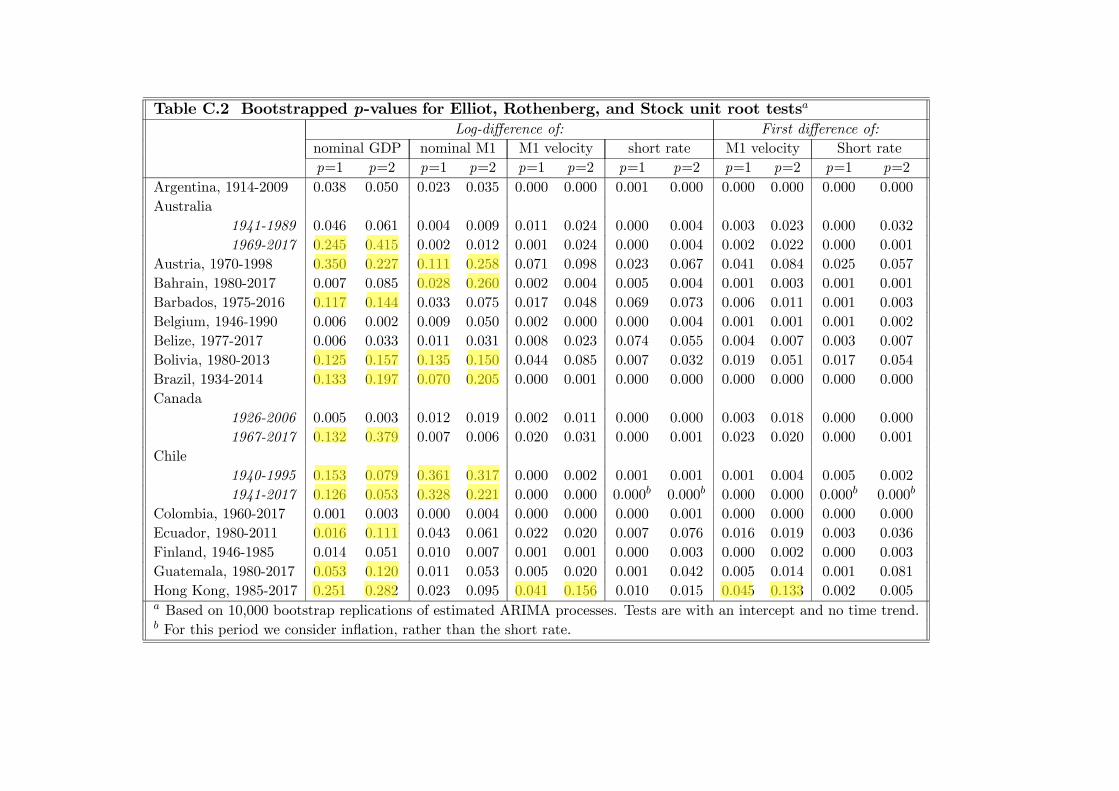
Table C.1 reports bootstrapped p-values3 for Elliot, Rothenberg, and Stock (1996)unit root tests for either the levels or the logarithms of M1 velocity and the shortrate, and for the logarithms of nominal M1 and nominal GDP,4 and Table C.2 reportsthe corresponding set of results for either the first di§erences or the log-di§erencesof the series. For the logarithms of nominal GDP and nominal M1, which exhibitobvious trends, tests are based on models including an intercept and a time trend.5

For (the logarithms of) the short rate and velocity, on the other hand, they are based

3For any of the series, p-values have been computed by bootstrapping 10,000 times estimatedARIMA(p,1,0) processes. In all cases, the bootstrapped processes are of a length equal to the seriesunder investigation. As for the lag order, p, since, as it is well known, results from unit root testsmay be sensitive to the specific lag order which is being used, for reasons of robustness we considertwo alternative lag orders, either 1 or 2 years.

4The reason for not considering tests based on the levels of nominal M1 and nominal GDP isthat either series’ level is manifestly characterized by exponential-type growth. This would not be aproblem if Elliot et al.’s tests allowed for the alternative of stationarity around an exponential trendrather than a linear one. Since this is not the case, for both GDP and M1 we are compelled to onlyconsider tests based on the logarithms.

5The reason for including a time trend is that, as discussed, for example, by Hamilton (1994, pp.501), the model used for unit root tests should be a meaningful one also under the alternative.

22

on models including an intercept but no time trend. For the short rate, the rationalefor not including a trend is obvious: the notion that nominal interest rates may followan upward path,6 in which they grow over time, is manifestly absurd.7 For velocity,on the other hand, things are at first sight less obvious. The reason for not includinga trend has to do with the fact that we are focusing here on a demand for moneyfor transaction purposes (so this argument holds for M1, but it would not hold forbroader aggregates). The resulting natural assumption of unitary income elasticitylogically implies that, if the demand for M1 is stable, M1 velocity should inherit thestochastic properties of the opportunity cost of money. In turn, this implies that thetype of tests we run for velocity should be the same as those for the nominal rate.The evidence in the two tables can be summarized as follows.First, there is overwhelming evidence of unit roots in any of the series, with the

bootstrapped p-values being near-uniformly greater than the 10% threshold which,throughout the entire paper, we take as our benchmark significance level and in mostcases markedly so.8 The handful of cases in which the null of a unit root is rejectedbased on either lag order has been highlighted, in Table C.1, in yellow.Second, for both the first di§erence and the log-di§erence of either velocity or the

short rate, the null of a unit root can be rejected almost uniformly, with the very fewcases in which this is not the case–so that the relevant series should be regarded,according to Elliot et al.’s (1996) tests, as I(2)–having been highlighted in yellow inTable C.2. Accordingly, for these cases we will not run cointegration tests. As fornominal M1 and especially nominal GDP, on the other hand, the opposite is true,with the null of a unit root not being rejected most of the time. In all of these cases,we will therefore eschew unrestricted specifications for the logarithms of nominal M1,nominal GDP, and a short rate.

D Details of the Bootstrapping Procedures

As for the Johansen test, we bootstrap trace and maximum eigenvalue statistics viathe procedure proposed by Cavaliere et al. (2012; henceforth, CRT). In a nutshell,CRT’s procedure is based on the notion of computing critical and p-values by boot-strapping the model that is relevant under the null hypothesis. This means that for

6The possibility of a downward path is ruled out by the zero lower bound.7This does not rule out the possibility that, over specific sample periods in which inflation ex-

hibits permanent variation (such as post-WWII samples dominated by the Great Inflation episode),nominal interest rates are I(1), too. Rather, by the Fisher e§ect, we should expect this to be thecase. Historically, however, a unit root in inflation has been the exception rather than the rule; seeBenati (2008).

8In a few cases, results based on the two alternative lag orders we consider produce contrastingevidence. This is the case, for example, for the logarithm of nominal GDP for Austria, the Barbadosislands, Hong Kong, Canada (1967-2017), Israel, and South Korea. In these cases, we regard the nullof a unit root as not having been convincingly rejected, and in what follows we therefore proceedunder the assumption that these series are I(1).

23

tests of the null of no cointegration against the alternative of one or more cointe-grating vectors, the model that is being bootstrapped is a simple, noncointegratedVAR in di§erences. For the maximum eigenvalue tests of h versus h+1 cointegratingvectors, on the other hand, the model that ought to be bootstrapped is the VECMestimated under the null of h cointegrating vectors. All of the technical details canbe found in CRT, to which the reader is referred. We select the VAR lag order as themaximum9 between the lag orders chosen by the Schwartz and the Hannan-Quinncriteria10 for the VAR in levels.As for the Wright (2000) test, since the test has been designed to be equally

valid for data-generating processes (DGPs) featuring either exact or near unit roots,we consider two alternative bootstrapping procedures, corresponding to either of thetwo possible cases. (In practice, as a comparison between the results reported inTable 2 in the text and in Table E.1 in Appendix E makes clear, the two proceduresproduce nearly identical results.) The former procedure involves bootstrapping–asdetailed in CRT and briefly recounted in the previous paragraph–the cointegratedVECM estimated (based on Johansen’s procedure) under the null of one cointegrationvector. This bootstrapping procedure is the correct one if the data feature exact unitroots. For the alternative possible case in which velocity and the short rate are nearunit root processes, we proceed as follows. Based on the just-mentioned cointegratedVECM estimated under the null of one cointegration vector, we compute the impliedVAR in levels. By construction, this VAR has one–and only one–eigenvalue equalto 1. Bootstrapping this VAR would obviously be exactly equivalent to bootstrappingthe underlying cointegrated VECM, that is, it would be the correct thing to do if thedata featured exact unit roots. Since, on the other hand, here we want to bootstrapunder the null of a near unit root cointegrated DGP, we turn such exact unit rootVAR in levels into its near unit root correspondent, by “shrinking down” the singleunitary eigenvalue to λ=1-0.5·(1/T ), where T is the sample length. In particular,we do that via a small perturbation of the parameters of the VAR matrices Bj’sin the cointegrated VECM representation ∆Yt = A + B1∆Yt−1 + ... + Bp∆Yt−p +GYt−1+ ut, where Yt collects (the logarithms of) M1 velocity and the short rate, andthe rest of the notation is obvious. By only perturbating the elements of the VARmatrices Bj’s–leaving unchanged the elements of the matrix G (and therefore boththe cointegration vector and the loading coe¢cients)–we make sure that both thelong-run equilibrium relationship between velocity and the short rate, and the way inwhich disequilibria in such relationship map into subsequent adjustments in the twoseries, remain unchanged. The bootstrapping procedure we implement for the second

9We consider the maximum between the lag orders chosen by the SIC and HQ criteria becausethe risk associated with selecting a lag order smaller than the true one (model misspecification) ismore serious than the one resulting from choosing a lag order greater than the true one (overfitting).10On the other hand, we do not consider the Akaike Information Criterion since, as discussed

by Luetkepohl (1991), for example, for systems featuring I(1) series, the AIC is an inconsistent lagselection criterion, in the sense of not choosing the correct lag order asymptotically.

24

possible case in which the processes feature near unit roots is based on bootstrappingsuch near unit root VAR.We now turn to discussing Monte Carlo evidence on the performance of the two

bootstrapping procedures.

D.1 Monte Carlo evidence on the performance of the twobootstrapping procedures

D.1.1 Evidence for Johansen’s test of the null of no cointegration

Table D.1 in this appendix reports Monte Carlo evidence on the performance of thebootstrapping procedure for Johansen’s trace tests11 proposed by CRT.12 We performthe Monte Carlo simulations based on two types of DGP, featuring no cointegrationand cointegration, respectively. As for the DGP featuring no cointegration, we simplyconsider two independent random walks. As for the one featuring cointegration, weconsider the following bivariate process:

yt = yt−1 + ϵt, with ϵt s i.i.d. N(0, 1) (D.1)

xt = yt + ut (D.2)

ut = ρut−1 + vt, with 0 ≤ ρ < 1, vt s i.i.d. N(0, 1). (D.3)

As for ρ, we consider six possible values, corresponding to alternative ranges of per-sistence of the cointegration residual between the three series, that is, ρ = 0, 0.25, 0.5,0.75, 0.9, and 0.95. There are two reasons for using this specific DGP. First, it cap-tures the essence of the problem at hand. Here we have two I(1) series–M1 velocityand a short rate–whose long-run dynamics might obey a cointegration relationship.Second, by parameterizing the extent of persistence of the deviation from the long-run equilibrium relationship, we can e§ectively explore how the performance of thetest depends on such persistence, even in very large samples. This is key because, aswe document in Online Appendix H, real-world (“candidate”) cointegration residualsare indeed very highly persistent. Intuitively, for the reasons discussed by Engle andGranger (1987), we would expect that, ceteris paribus, the higher the persistence ofthe cointegration residual, the more di¢cult it is for any statistical test to detectcointegration. As we will see, this is indeed the case.

11Numerically near-identical evidence for Johansen’s maximum eigenvalue tests is not reportedfor reasons of space, but it is available upon request.12Extensive Monte Carlo evidence on the good performance of the CRT procedure was already

provided by CRT themselves in their original paper. Benati (2015) also provided some (much morelimited) evidence conditional on the specific DGPs he was interested in. The rationale for providingadditional evidence here is the same as Benati (2015), that is, looking at how the procedure performsconditional on the DGPs we are interested in here.

25

Details of the Monte Carlo simulations are as follows. For either DGP, we considerfive alternative sample lengths, T = 50, 100, 200, 500, and 1,000. For each combina-tion of values of ρ and T , we generate 5,000 artificial samples of length T+100, andwe then discard the first 100 observations in order to eliminate dependence on initialconditions (which we set to 0 for either series). For each individual simulation, webootstrap the relevant test statistic based on 2,000 bootstrap replications.Table D.1 reports the evidence for Johansen’s trace test of the null of no cointe-

gration against the alternative of one or more cointegration vectors. Specifically, thetable reports, for either DGP, the sample length and (for the DGP featuring cointe-gration) the value of ρ; and the fraction of replications for which no cointegration isrejected at the 10% level. The following main findings clearly emerge from the table.First, in line with the evidence reported by both CRT and Benati (2015), the pro-

cedure performs remarkably well conditional on DGPs featuring no cointegration. Akey point that ought to be stressed is that the specific sample length used in the simu-lations does not appear to make any material di§erence for the final results, with thefractions of rejections ranging between 0.098 and 0.119 (with the ideal one being 0.1).This is testimony to the power of bootstrapping, which is capable of automaticallycontrolling for the specific characteristics of the DGP under investigation.Second, when the DGP does feature cointegration, ideally we would like the test

to reject as much as possible. As the lower part of the table shows, the procedureindeed performs very well if ρ is small. If ρ = 0, for example, cointegration is alreadydetected 100% of the time for T = 100, whereas if ρ = 0.5, it is detected 88.2%of the time for T = 100, and a sample length of T = 200 is already su¢cient todetect cointegration 100% of the time. As ρ increases, however, the performancedeteriorates. The intuition for this is straightforward: as the cointegration residualbecomes more and more persistent, it gets closer and closer to a random walk (inwhich case there would be no cointegration), and the procedure therefore needs largerand larger samples to detect the truth (that the residual is highly persistent butultimately stationary). In particular, as ρ increases, the fraction of rejections tendsto converge, for each sample size, to the fraction of rejections under the DGP featuringno cointegration. This is especially apparent for T = 50 or 100, with the fractionsbeing equal to 0.114 and 0.120, respectively. In the limit, for ρ ! 1, the procedurewill tend to reject 10% of the time.

Comparison with theMonte Carlo evidence of Cavaliere et al. (2012) Thisevidence is qualitatively and also quantitatively in line with the Monte Carlo evidencereported in CRT’s Tables I and II, pp. 1731-1732. Although the DGPs they used(either noncointegrated VARs or cointegrated VECMs featuring one cointegrationvector) were di§erent from the DGPs used herein, their results and ours turn out tobe very close. Specifically, the results are as follows:

• The results in panel (b) of their Table I illustrate the excellent performanceof their bootstrapping procedure for tests of the null of no cointegration when

26

the true DGP features no cointegration. In line with the evidence reportedin the first row of our Table E.1, their results illustrate how, at the 5% level,the empirical rejection frequencies (henceforth, ERF) are quite close to 5%irrespective of the sample size.

• Panel (a) in the same table reports qualitatively and quantitatively similarevidence for the maximum eigenvalue test of 1 versus 2 cointegrating vectors,conditional on DGPs featuring one cointegrating vector.

• Finally, CRT’s Table II reports evidence on the ability of the sequential boot-strapped procedure to select the correct cointegration rank, which in their ex-periments is one (see the columns under the heading “Bootstrap (CRT)”). Thoseresults are in line with the ones reported in our Table 1 in the main text con-ditional on DGPs featuring one cointegration vector. In either case, the largerthe sample size, the more frequently CRT’s procedure detects the truth, withERFs converging toward 1 for su¢ciently large samples. In comparatively smallsamples (e.g., for T = 50), ERFs are typically much below one–as we show,the more so, the more persistent is the cointegration residual.13

The bottom line is that our Monte Carlo evidence, although based on a set ofDGPs that have been specifically tailored to the problem at hand, is in fact exactlyin line, both qualitatively and quantitatively, with the evidence reported in CRT.

Summing up The proceeding can be summarized as follows:

• If the true DGP features no cointegration, CRT’s procedure performs remark-ably well irrespective of the sample size.

• If, however, the true DGP features cointegration, Johansen’s tests–even boot-strapped as in CRT–perform well only if the persistence of the cointegrationresidual is su¢ciently low and/or the sample size is su¢ciently large. If, onthe other hand, the cointegration residual is persistent and the sample size issmall, the procedure will fail to detect cointegration a nonnegligible fraction ofthe time. For example, with T = 100, cointegration will be detected 43.3% ofthe time if ρ = 0.75 and just 12.0% of the time if ρ = 0.95.

13Di§erent from the present work, CRT do not explore how the persistence of the cointegrationresidual a§ects the performance of their procedure. The results reported in their Table II, however,are quantitatively in line with ours. We found this in the following way. We simulated their VECMconditional on one cointegration vector 10,000 times for samples of length T = 10,000, and for eachsimulation we computed the implied cointegration residual, and based on it we estimated an AR(4)process (in fact, given the nature of their DGP, an AR(2) would have been enough). The sum of theAR coe¢cients is our measure of persistence. For their benchmark case of δ=0.1, both the meanand the median of the distribution were equal to 0.61. From their Table II, we can see that for δ=0.1and T = 50, the ERF is 49.0%. In Table 1 of the main text we report, for T = 50 and ρ=0.5, anERF of 35%.

27

All of this means that if Johansen’s tests do detect cointegration, we should havea reasonable presumption that cointegration is indeed there. If, on the other hand,they do not detect it, a possible explanation is that the sample period is too shortand/or the cointegration residual is highly persistent.

D.1.2 Evidence for Wright’s (2000) test of the null of cointegration

Table D.2 reports evidence for the two bootstrapping procedures we use for Wright’stest. Specifically, the top portion of the table reports evidence for the case of exactunit roots, with the true DGP that is being simulated being given by (D.1)-(D.3),and the bootstrapping procedure being the first one discussed in the second para-graph of this appendix, that is, being based on bootstrapping the VECM estimatedconditional on one cointegration vector. The second portion of Table D.2 reports thecorresponding Monte Carlo evidence for the near unit root case. Here the DGP thatis being simulated is the near unit root version of (D.1)-(D.3), that is, the DGP thatis obtained when the random walk (D.1) is replaced with

yt = λyt−1 + ϵt, with ϵt s i.i.d. N(0, 1) (D.1)

with λ=1-0.5·(1/T ), where T is the sample length. For each single bootstrappedreplication, the test statistics are bootstrapped based on the second procedure dis-cussed in the second paragraph of this appendix, that is, by bootstrapping the nearunit root VAR in levels obtained by “shrinking down” to λ=1-0.5·(1/T ) the unitaryeigenvalue of the VAR in levels implied by the VECM estimated conditional on onecointegration vector.All of the details of the Monte Carlo simulations are exactly the same as for

Johansen test (grids of values for ρ and T , number of Monte Carlo simulations, andnumber of bootstrap replications). As a comparison between the top and bottomportions of Table D.2 shows, evidence for the two cases of exact and near unit rootsis virtually identical and can be summarized as follows:14

First, if the true DGP features cointegration, the procedure works remarkablywell if the sample size is su¢ciently long, the persistence of the cointegration residualis su¢ciently low, or both. For example, for T = 1,000, the empirical rejectionfrequencies (ERFs) at the 10% level range between 0.103 and 0.116, very close to theideal of 0.1. As the sample size decreases, however, the ERFs systematically increase.For T = 200, for example, the ERF is still equal to 0.105 for ρ = 0.75, but for ρ =0.95 it becomes equal to 0.127. For T = 50 the ERF is still reasonably close to 0.1for ρ = 0.5, but for ρ = 0.9 it is already equal to 0.181, and it further increases to0.206 for ρ = 0.95.Second, if the true DGP features no cointegration (i.e., two independent random

walks), the ERFs range between 0.200 and 0.227 depending on sample size.

14In what follows, all of the numbers mentioned pertain to the case of exact unit roots.

28

Summing up The proceeding can be summarized as follows:

• If the true DGP features cointegration, in the case of either exact or near unitroots, the respective bootstrapping procedures perform remarkably well if thesample size is su¢ciently long, the persistence of the cointegration residual issu¢ciently low, or both. However, if the sample is su¢ciently short and thecointegration residual is su¢ciently persistent, the null of cointegration will beincorrectly rejected, in the worst possible scenario analyzed in the Monte Carloexperiment (T = 50 and ρ = 0.95) at about twice the nominal size. The expla-nation for this is straightforward, and it is, in fact, in line with the previouslymentioned point made by Engle and Granger (1987): when the cointegrationresidual is highly persistent, only su¢ciently long samples allow the test to de-tect the truth, that is, that the deviation between the two series is ultimatelytransitory, so that they are in fact cointegrated. On the other hand, under thesecircumstances the shorter the sample period, the more likely it will be to mis-takenly infer that the deviation between the two series is, in fact, permanent,so that they are not, in fact, cointegrated.

• If, on the other hand, the true DGP features no cointegration, in the case ofeither exact or near unit roots, the test will reject the null at roughly twice thenominal size.

A key implication is that, in fact, lack of rejection of the null of no cointegrationdoes not represent very strong evidence that cointegration truly is in the data. Since inthe case of two independent random walks (or their near unit root correspondent) thenull of cointegration is rejected about one time out of five irrespective of sample length,an alternative interpretation is simply that the data do not feature cointegration, butthe test is not capable of detecting this.

E Additional Results from Wright’s (2000) Testfor M1 Velocity and the Short Rate

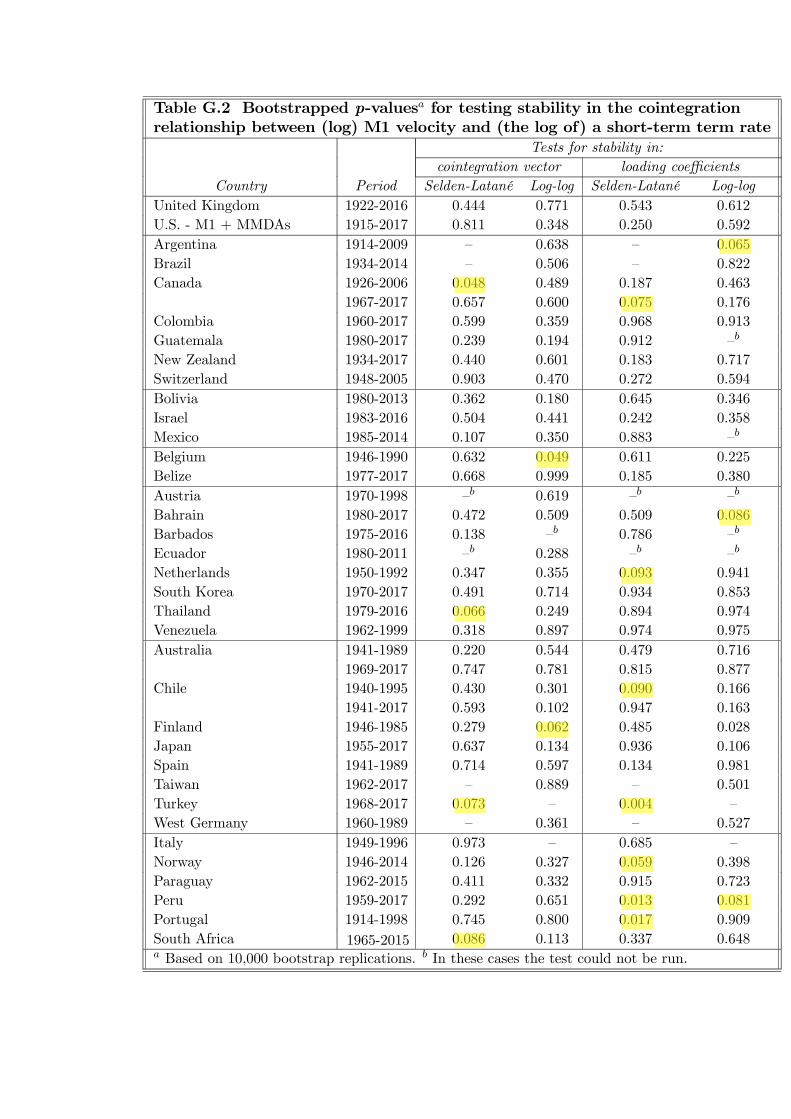
Table E.1 in this appendix reports results from Wright’s (2000) test based on thesecond bootstrapping procedure previously discussed in Appendix D, that is, basedon bootstrapping the near unit root VAR, which has been obtained by perturbatingthe coe¢cients of the AR matrices of the cointegrated VECM produced by Johansen’sprocedure (estimated conditional on one cointegration vector) in such a way that theunitary eigenvalue is “shrunk down” to its near unit root equivalent 1-0.5·(1/T ),where T is the sample length. Evidence is nearly identical to that reported in Table 2in the main text, and it points towards the presence of cointegration across the boardbetween (the logarithms of) M1 velocity and the short rate.

29

F Unrestricted Tests of the Null of No Cointegra-tion

Table F.1 in this appendix reports results from Johansen’s cointegration test based onunrestricted specifications featuring the logarithms of M1, nominal GDP, and a shortrate. On the other hand, we do not perform the corresponding set of tests based onthe levels of the three series, since two of them–M1 and nominal GDP–exhibit ob-vious exponential (that is, nonlinear) trends, which makes linear cointegration tests,such as Johansen’s, Shin’s (1994), or Wright’s (2000), pointless within the presentcontext. Out of 18 samples, the tests detect cointegration only in 5 cases. Results forthe United Kingdom, the United States, Argentina, Canada, Switzerland, Bolivia,Belize, Australia, Spain, and South Africa are in line with those based on the cor-responding restricted specification for the logarithms of velocity and the short ratein Table 1 in the main text. On the other hand, for Colombia, New Zealand, andBelgium, where the tests based on velocity and the short rate did detect cointegra-tion, the corresponding unrestricted tests in Table F.1 do not reject the null of nocointegration. A possible and likely explanation for this contrast is that failure toimpose the (true) restriction of unitary income elasticity decreases the power of thetest, leading it to incorrectly not reject the null. For Israel, Portugal, and Norway,relaxation of the constraint of unitary income elasticity leads the unrestricted test todetect cointegration, in contrast to the results from the unrestricted test in Table 1.In light of the evidence of a remarkably strong correlation between the logarithmsof M1 velocity and the short rate for Israel in Figure 5 of the main text, and of thecorresponding lack of any correlation between the levels of the two series, we regardthe results for this country in either table as a fluke, likely due to the short samplelength.

G Testing for Stability in Cointegration Relation-ships

In Section 6.2 in the main text of the paper we test for either breaks or, more generally,time variation in cointegration relationships based on the three tests discussed byHansen and Johansen (1999): Two Nyblom-type tests for stability in the cointegrationvector and the vector of loading coe¢cients, respectively; and a fluctuation test,which is essentially a joint test for time-variation in the cointegration vector and theloadings.

30

G.1 Monte Carlo evidence on the performance of Hansenand Johansen’s (1999) tests

Table G.1 in this appendix reports Monte Carlo evidence on the performance of thethree tests conditional on bivariate cointegrated DGPs featuring no time variation ofany kind, for alternative sample lengths, and alternative degrees of persistence of thecointegration residual, which is modelled as an AR(1). Specifically, the DGP is givenby

yt = yt−1 + ϵt, with ϵt s i.i.d. N(0, 1) (G.1)

xt = yt + ut (G.2)

with the cointegration residual being

ut = ρut−1 + vt, with 0 ≤ ρ < 1, vt s i.i.d. N(0, 1). (G.3)

We consider T = 50, 100, 200, and ρ = 0, 0.25, 0.5, 0.75, 0.9, 0.95, and for eachcombination of T and ρ, we stochastically simulate the DGP based on each simulation,we perform either of the three tests on [yt xt]0, bootstrapping them as in Cavaliere et al.(2012) conditional on one cointegration vector (i.e., the true number of cointegrationvectors in the DGP), based on 1,000 bootstrap replications. In performing of thethree tests, we set the “trimming parameter” to the standard value in the literatureof 0.15. For each combination of T and ρ, we perform 1,000 Monte Carlo simulations.The table reports, for each combination of T and ρ, the fraction of Monte Carlosimulations for which stability is rejected at the 10% level.The main results in the table can be summarized as follows. The two Nyblom-type

tests exhibit an overall reasonable performance, incorrectly rejecting the null of notime variation, most of the time, at roughly the nominal size. Crucially, this is the caseirrespective of the sample length and of the persistence of the cointegration residual.The fluctuation test, on the other hand, exhibits a good performance only if thepersistence of the cointegration residual is low. The higher the residual’s persistence,however, the worse the performance, so that, for example, when the AR root of theresidual is equal to 0.95, for a sample length T = 50, the test rejects at roughlytwice the nominal size. This is clearly problematic since–as we mentioned in themain text, and we discuss more in detail in Appendix H –cointegration residualsare typically moderately to highly persistent. Because of this, in the main text wetherefore focus on the results from the two Nyblom-type tests, whereas we eschewresults from fluctuations tests (these results are, however, reported in table G.4).

G.2 Evidence on the stability of cointegration relationships

Table G.2 in this appendix reports the results from Hansen and Johansen’s (1999)Nyblom-type tests for breaks in either the cointegration vector or the loading coe¢-cients in the cointegrated VECMs estimated (based on Johansen’s estimator) condi-tional on one cointegration vector. Specifically, the table reports p-values for testing

31

stability in either feature of the cointegrated VECM, which have been bootstrappedas in Cavaliere et al. (2012), that is, based on the model estimated conditional onone cointegration vector. The main result emerging from the table is that evidenceof breaks in either feature is weak to nonexistent. In particular, focusing on thecointegration vector–which, for the purpose of addressing the question of whetherthere is a stable long-run relationship between velocity and the short rate is clearlythe key feature–at the 10% level we detect a break in four cases (Canada, Thailand,Turkey, and South Africa) based on the Selden-Latané specification, and in just twocases (Belgium and Finland) based on the log-log. Evidence of breaks in the vectorof loading coe¢cients is slightly stronger–seven instances based on Selden-Latanéand three based on log-log–but breaks in this feature bear no implication for thepresence of a stable long-run relationship between the two series, as they uniquelyhinge upon the way the system converges toward the long-run equilibrium.Table G.3 reports, for the handful of cases in which a break in either feature

has been detected, the estimated break dates, together with the values which themodel feature which has been subject to breaks–either the cointegration vector orthe loading coe¢cients–has taken in the two subsamples.Finally, Table G.4 reports p-values (again, bootstrapped as in Cavaliere et al.

(2012) based on the VECM estimated conditional on one cointegration vector) forHansen and Johansen’s (1999) fluctuations tests based on the cointegrated VECM.Results are qualitatively in line with those for the two just-discussed Nyblom-typetests for breaks in either the cointegration vector or the loading coe¢cients, withevidence of time variation identified only in a handful of cases.

H Evidence on the Persistence of ‘Candidate’ Coin-tegration Residuals

Tables H.1 and H.2 in this appendix report Hansen’s (1999) “grid bootstrap” median-unbiased (henceforth, MUB) estimates of the sum of the AR coe¢cients in AR(2)representations for the “candidate cointegration residuals” in our dataset.15 By “can-didate cointegration residual” (henceforth, CCR), we mean the linear combinationof the I(1) variables in the system which will indeed be regarded as a cointegra-tion residual if cointegration is detected.16 For reasons of robustness, for either theSelden-Latané specification (Table H.1) or the log-log (Table H.2), we consider two

15Results are based on 2,000 bootstrap replications for each possible value of the sum of the ARcoe¢cients in the grid. Bootstrapping has been performed as in Diebold and Chen (1996). Forreasons of robustness, we report results based on two alternative estimators of the cointegrationvector, Johansen’s, and Stock and Watson’s (1993).16We label it as the candidate cointegration residual because, as the Monte Carlo evidence in

the previous section has shown, if a residual is highly persistent, cointegration might well not bedetected even if it is present, which would prevent the candidate from being identified as a truecointegration residual.

32

alternative estimators of the cointegration residual, either Johansen’s or Stock andWatson’s (1993).Evidence points toward both a nonnegligible degree of persistence of the CCRs

and a wide degree of heterogeneity across countries. Focusing on results based on thelog-log specification, the MUB estimate based on Johansen’s estimator of the cointe-gration vector–let’s label it as ρJ

MUB–ranges from a minimum of 0.27 for Belize to

a maximum of 1.17 for the Barbados islands. By classifying the ρJMUB

’s, in an admit-tedly arbitrary fashion, as “highly persistent” (ρJ

MUB≥0.8), “moderately persistent”

(0.4< ρJMUB

<0.8), and “not very persistent” (ρJMUB

≤0.4), we end up with 22 ρJMUB

’sin the first group, 14 in the second, and 4 in the third. Results based on Stockand Watson’s estimator are qualitatively the same, with the three groups comprisingrespectively 25, 13, and 2 countries.

I Evidence on the Functional Form

Figures I.1 and I.2 provide simple, informal evidence on which specifications–Selden-Latané or log-log –provides the most plausible description of the data at low and,respectively, high interest rates. In both figures, the top row shows the levels ofM1 velocity and the short rate, and the bottom row shows the logarithms of thetwo series. The evidence in the two rows therefore corresponds to a Selden-Latanéand, respectively, a log-log specification for the demand for real M1 balances withunitary income elasticity, linearly relating either the level or the logarithm of M1velocity to the level or, respectively, the logarithm of the short rate. Figure I.2reports evidence for all of the countries that we classified as high-inflation countries,arranged in descending order according to the level of the interest rate. For reasonsof space, Figure I.2 only reports evidence for 10 of the remaining countries. This ishowever without loss of generality, as this evidence is representative of the entire setof low-inflation countries (this evidence is available upon request).Two broad patterns emerge from Figures I.1 and I.2. First, at low interest rates

the Selden-Latané specification appears to provide a more plausible description ofthe data than the log-log, in the sense that, in several cases, the correlation betweenthe levels of velocity and the short rate is manifestly stronger than that betweenthe logarithms of the two series. This is especially clear for the United States, theUnited Kingdom, Switzerland, the Barbados islands, and, to a certain extent, Belize,whereas evidence for Japan is slightly weaker, and it crucially hinges on the periodsince the beginning of the new millennium. On the other hand, for countries suchas Canada, South Korea, the Netherlands, and New Zealand, neither specificationis manifestly superior, as the correlation between the levels of the series appears asequally strong as that between their logarithms. Another way of stating this is that,among low-inflation rate countries, in no single case does the log-log specification pro-vide a manifestly better description of the data than the Selden-Latané specification,

33

whereas in several cases the data clearly prefer the latter to the former.Second, at high or very high interest rates, the opposite is true: in no single case is

the Selden-Latané specification clearly preferred by the data, whereas in a few cases,the log-log specification provides a manifestly better description of the data. Thisis especially clear for Israel, Argentina, and Brazil, and to a lesser extent for Chile,Bolivia, and Ecuador, whereas for Turkey and Venezuela, the correlations betweenthe levels and, respectively, the logarithms of the two series appear as equally strongor weak, depending on the period. Interestingly, the data’s preference for the log-log specification appears stronger the higher the level of the interest rate (which isreported, in the top row, in the right-hand side scale in either panel in black), whereasit becomes progressively weaker for countries characterized by comparatively lowerinterest rates.

34

References

Baffigi, A. (2011): “Italian National Accounts: A Project of Banca d’Italia, ISTATand University of Rome Tor Vergata,” Economic History Working Papers, Bancad’Italia, n. 18.

BancadItalia (2013): “Tavole Storiche, Indicatori Monetari e Finanziari,” Dicem-bre 2013.

Barciela-LÃSpez, C., A. Carreras, and X. Tafunell (2005): EstadÃŋsticasHistÃsricas de EspaÃsa: Siglos XIX-XX, Vol. 3. Fundacion BBVA.

Barkai, H., and N. Liviatan (2007): The Bank of Israel Volume 1: A MonetaryHistory. New York: Oxford University Press.

Benati, L. (2008): “Investigating Inflation Persistence Across Monetary Regimes,”Quarterly Journal of Economics, 123(3), 1005—1060.

(2015): “The Long-Run Phillips Curve: A Structural VAR Investigation,”Journal of Monetary Economics, 76, 15—28.

Bernanke, B. S., M. Gertler, and M. Watson (1997): “Systematic MonetaryPolicy and the E§ects of Oil Price Shocks,” Brookings Papers on Economic Activity,1997(1), 91—157.

Boeschoten, W. (1992): Hoofdlijnen van de economische geschiedenis van Neder-land 1900-1990. Amsterdam: NIBE.

deJong, A. (1967):.

Diebold, F. X., and C. Chen (1996): “Testing Structural Stability with Endoge-nous Breakpoint: A Size Comparison of Analytic and Bootstrap Procedures,” Jour-nal of Econometrics, 70(1), 221—241.

Elliot, G., T. J. Rothenberg, and J. H. Stock (1996): “E¢cient Tests for anAutoregressive Unit Root,” Econometrica, 64(4), 813—836.

Fratianni, M., and F. Spinelli (1997): A Monetary History of Italy. Cambridge:Cambridge University Press.

Furlong, K. (2001): “The Montreal Gazette Call Loan Rate, 1871-1907,” CanadianJournal of Economics, 34(1), 165—173.

Haavisto, T. (1992): Money and Economic Activity in Finland, 1866-1985. LundEconomic Studies.

35

Hansen, H., and S. Johansen (1999): “Some Tests for Parameter Constancy inCointegrated VAR Models,” Econometrics Journal, 2(2), 306—333.

Hills, S., and R. T. N. Dimsdale (2010): “The UK Recession in Context: WhatDo Three Centuries of Data Tell Us?,” Bank of England Quarterly Bulletin, (2010Q4), 277—291.

Homer, S., and R. Sylla (2005): A History of Interest Rates. New York: JohnWiley.

Judson, R. (2017): “The Death of Cash? Not So Fast: Demand for U.S. Currencyat Home and Abroad, 1990-2016,” Federal Reserve Board, Division of InternationalFinance Working Paper, forthcoming.

Junguito, R., and H. RincÃSn (2007): “La polÃŋtica fiscal en el siglo XX enColombia,” in J. Robinson and M. Urrutia (eds.), EconomÃŋa Colombiana delSiglo XX: Un AnÃalisis Cuantitativo, Banco de la RepÃzblica y Fondo de CulturaEconÃsmica, Colombia, pp. —.

Klovland, J. T. (2004): “Monetary aggregates in Norway 1819-2003,” in ßyvindEitrheim, Jan T. Klovland and Jan F. Qvigstad, eds., Historical Monetary Statis-tics for Norway 1819ÂU2003, Norges Bank, Occasional Paper N. 35/2004.

Luetkepohl, H. (1991): Introduction to Multiple Time Series Analysis, 2nd ed.Berlin: Springer-Verlag.

Mata, E., and N. Valerio (2011): The Concise Economic History of Portugal: AComprehensive Guide. Coimbra: Almedina.

Metcalf, C., A. Redish, and R. Shearer (1996): “New Estimates of the Cana-dian Money Stock: 1871-1967,” University of British Columbia Discussion PaperNo. 96-17, July 1996.

Mitchell, B. R. (2007): International Historical Statistics: Africa, Asia, and Ocea-nia, 1750-2000. New York: Palgrave Macmillan.

Muscatelli, A., and F. Spinelli (2000): “The Long-Run Stability of the Demandfor Money: Italy 1861-1996,” Journal of Monetary Economics, 45(3), 717—739.

Officer, L. H., and S. H. Williamson (2015): “The Annual Con-sumer Price Index for the United States, 1774-2014,” available at:http://www.measuringworth.com/uscpi/.

SaintMarc, M. (1983): Histoire Monetarie de la France, 1880-1980. Paris, PressesUniversitaires de la France.

36

Shearer, R. A., and C. Clark (1984): “Canada and the Interwar Gold Stan-dard, 1920-35: Monetary Policy without a Central Bank,” in M. D. Bordo andA. J. Schwartz, eds., A Retrospective on the Classical Gold Standard, 1821-1931,University of Chicago Press, pp. 277—310.

Smits, J.-P., P. Woltjer, and D. Ma (2009): “A Dataset on Comparative His-torical National Accounts, ca. 1870-1950: A Time-Series Perspective,” .

Tamaki, N. (1995): Japanese Banking: A History 1859-1959. Cambridge: Cam-bridge University Press.

37

Table C.1 Bootstrapped p-values for Elliot, Rothenberg, and Stock unit root testsd

Logarithm of: Level of:nominal GDP nominal M1 M1 velocity short rate M1 velocity Short ratep=1 p=2 p=1 p=2 p=1 p=2 p=1 p=2 p=1 p=2 p=1 p=2

Argentina, 1914-2009 0.227 0.903 0.201 0.847 0.686 0.746 0.316 0.332 0.562 0.724 0.012 0.009Australia

1941-1989 0.771 0.607 0.622 0.978 0.931 0.854 0.784 0.872 0.947 0.932 0.915 0.9841969-2017 0.100 0.465 0.955 0.982 0.856 0.884 0.905 0.966 0.840 0.872 0.596 0.815

Austria, 1970-1998 0.024 0.128 0.125 0.685 0.970 0.977 0.509 0.351 0.961 0.968 0.361 0.198Bahrain, 1980-2017 0.525 0.466 0.368 0.059 0.652 0.769 0.448 0.365 0.544 0.689 0.335 0.216Barbados, 1975-2016 0.060 0.114 0.572 0.317 0.802 0.748 0.992 0.968 0.552 0.528 0.418 0.428Belgium, 1946-1990 0.861 0.885 0.211 0.236 0.036 0.166 0.130 0.670 0.497 0.733 0.414 0.664Belize, 1977-2017 0.234 0.580 0.302 0.138 0.942 0.943 0.359 0.956 0.876 0.904 0.811 0.796Bolivia, 1980-2013 0.090 0.067 0.114 0.062 0.915 0.849 0.866 0.837 0.627 0.674 0.139 0.188Brazil, 1934-2014 0.304 0.581 0.258 0.559 0.747 0.744 0.367e 0.340e 0.554 0.534 0.007e 0.054e

Canada1926-2006 0.132 0.148 0.340 0.144 0.792 0.793 0.607 0.730 0.790 0.806 0.384 0.4791967-2017 0.087 0.330 0.022 0.032 0.971 0.969 0.792 0.824 0.854 0.837 0.617 0.681

Chile1940-1995 0.399 0.544 0.374 0.261 0.134 0.050 0.341 0.263 0.212 0.124 0.133 0.0901941-2017 0.922 0.913 0.906 0.692 0.450 0.303 0.205e 0.280e 0.302 0.127 0.047e 0.017e

Colombia, 1960-2017 0.107 0.974 0.090 0.942 0.244 0.263 0.827 0.905 0.162 0.199 0.718 0.822Ecuador, 1980-2011 0.493 0.375 0.097 0.188 0.877 0.815 0.793 0.870 0.795 0.761 0.437 0.727Finland, 1946-1985 0.288 0.100 0.057 0.071 0.776 0.594 0.541 0.521 0.914 0.897 0.512 0.511France, 1852-1913 0.001 0.001 0.896 0.891 0.642 0.803 0.051 0.037 0.522 0.743 0.027 0.040Guatemala, 1980-2017 0.950 0.965 0.992 0.993 0.672 0.585 0.596 0.508 0.622 0.520 0.573 0.516Hong Kong, 1985-2017 0.023 0.113 0.649 0.805 0.925 0.942 0.622 0.596 0.716 0.849 0.495 0.481d Based on 10,000 bootstrap replications of estimated ARIMA processes. Tests are with an intercept and a time trendfor the logarithms of nominal GDP and nominal M1, and with an intercept and no time trend for the other series.e For this period we consider inflation, rather than the short rate.

Table C.1 (continued) Bootstrapped p-values for Elliot, Rothenberg, and Stock unit root testsd

Logarithm of: Level of:nominal GDP nominal M1 M1 velocity short rate M1 velocity Short ratep=1 p=2 p=1 p=2 p=1 p=2 p=1 p=2 p=1 p=2 p=1 p=2

Japan, 1955-2017 0.144 0.623 0.090 0.314 0.945 0.936 0.697 0.748 0.749 0.757 0.578 0.566Israel, 1983-2016 0.000 0.144 0.001 0.001 0.792 0.040 0.477 0.065 0.318 0.257 0.106 0.057Italy, 1949-1996 0.794 0.889 0.993 0.945 0.333 0.648 0.857 0.899 0.234 0.643 0.805 0.848Mexico, 1985-2014 0.013 0.021 0.066 0.016 0.767 0.100 0.629 0.289 0.679 0.027 0.346 0.023Morocco, 1985-2017 0.119 0.193 0.400 0.654 0.319 0.267 0.806 0.717 0.059 0.048 0.761 0.595Netherlands, 1950-1992 0.985 0.996 0.703 0.783 0.100 0.194 0.194 0.450 0.232 0.297 0.243 0.347New Zealand, 1934-2017 0.960 0.981 0.479 0.527 0.825 0.814 0.665 0.651 0.815 0.798 0.351 0.337Norway, 1946-2014 0.955 0.995 0.123 0.153 0.898 0.880 0.802 0.755 0.846 0.837 0.774 0.723Paraguay, 1962-2015 0.719 0.920 0.733 0.706 0.426 0.447 0.032 0.067 0.342 0.394 0.125 0.249Peru, 1959-2017 0.767 0.857 0.738 0.794 0.599 0.427 0.488 0.564 0.600 0.419 0.112 0.116Portugal, 1914-1998 0.634 0.614 0.209 0.145 0.594 0.407 0.716 0.714 0.607 0.430 0.596 0.469South Africa, 1965-2015 0.995 0.995 0.751 0.839 0.918 0.927 0.289 0.484 0.875 0.882 0.283 0.332South Korea, 1970-2017 0.080 0.245 0.101 0.417 0.664 0.610 0.643 0.745 0.384 0.290 0.061 0.258Spain, 1941-1989 0.632 0.504 0.154 0.505 0.187 0.440 0.828 0.878 0.363 0.512 0.589 0.720Switzerland, 1948-2005 0.949 0.930 0.498 0.712 0.425 0.359 0.156 0.177 0.453 0.417 0.186 0.120Taiwan, 1962-2017 0.309 0.788 0.141 0.574 0.314 0.264 0.662 0.713 0.057 0.034 0.408 0.513Thailand, 1979-2016 0.291 0.867 0.944 0.936 0.907 0.916 0.619 0.523 0.890 0.898 0.589 0.418Turkey, 1968-2017 0.856 0.827 0.879 0.903 0.735 0.767 0.644 0.668 0.653 0.673 0.727 0.770United Kingdom, 1922-2016 0.140 0.805 0.080 0.391 0.831 0.746 0.926 0.942 0.779 0.728 0.345 0.575United States, 1915-2017

M1 0.702 0.385 0.482 0.158 0.626 0.783 0.443 0.248 0.578 0.697 0.302 0.319M1 + MMDAs 0.699 0.380 0.488 0.159 0.833 0.811 0.443 0.251 0.713 0.702 0.293 0.326

Venezuela, 1962-1999 0.521 0.752 0.738 0.817 0.574 0.729 0.744 0.730 0.543 0.786 0.691 0.706West Germany, 1960-1989 0.844 0.963 0.662 0.840 0.752 0.739 0.067 0.137 0.721 0.719 0.069 0.138d Based on 10,000 bootstrap replications of estimated ARIMA processes. Tests are with an intercept and a time trendfor the logarithms of nominal GDP and nominal M1, and with an intercept and no time trend for the other series.

Table C.2 Bootstrapped p-values for Elliot, Rothenberg, and Stock unit root testsd

Log-difference of: First difference of:nominal GDP nominal M1 M1 velocity short rate M1 velocity Short ratep=1 p=2 p=1 p=2 p=1 p=2 p=1 p=2 p=1 p=2 p=1 p=2

Argentina, 1914-2009 0.038 0.050 0.023 0.035 0.000 0.000 0.001 0.000 0.000 0.000 0.000 0.000Australia

1941-1989 0.046 0.061 0.004 0.009 0.011 0.024 0.000 0.004 0.003 0.023 0.000 0.0321969-2017 0.245 0.415 0.002 0.012 0.001 0.024 0.000 0.004 0.002 0.022 0.000 0.001

Austria, 1970-1998 0.350 0.227 0.111 0.258 0.071 0.098 0.023 0.067 0.041 0.084 0.025 0.057Bahrain, 1980-2017 0.007 0.085 0.028 0.260 0.002 0.004 0.005 0.004 0.001 0.003 0.001 0.001Barbados, 1975-2016 0.117 0.144 0.033 0.075 0.017 0.048 0.069 0.073 0.006 0.011 0.001 0.003Belgium, 1946-1990 0.006 0.002 0.009 0.050 0.002 0.000 0.000 0.004 0.001 0.001 0.001 0.002Belize, 1977-2017 0.006 0.033 0.011 0.031 0.008 0.023 0.074 0.055 0.004 0.007 0.003 0.007Bolivia, 1980-2013 0.125 0.157 0.135 0.150 0.044 0.085 0.007 0.032 0.019 0.051 0.017 0.054Brazil, 1934-2014 0.133 0.197 0.070 0.205 0.000 0.001 0.000 0.000 0.000 0.000 0.000 0.000Canada

1926-2006 0.005 0.003 0.012 0.019 0.002 0.011 0.000 0.000 0.003 0.018 0.000 0.0001967-2017 0.132 0.379 0.007 0.006 0.020 0.031 0.000 0.001 0.023 0.020 0.000 0.001

Chile1940-1995 0.153 0.079 0.361 0.317 0.000 0.002 0.001 0.001 0.001 0.004 0.005 0.0021941-2017 0.126 0.053 0.328 0.221 0.000 0.000 0.000e 0.000e 0.000 0.000 0.000e 0.000e

Colombia, 1960-2017 0.001 0.003 0.000 0.004 0.000 0.000 0.000 0.001 0.000 0.000 0.000 0.000Ecuador, 1980-2011 0.016 0.111 0.043 0.061 0.022 0.020 0.007 0.076 0.016 0.019 0.003 0.036Finland, 1946-1985 0.014 0.051 0.010 0.007 0.001 0.001 0.000 0.003 0.000 0.002 0.000 0.003Guatemala, 1980-2017 0.053 0.120 0.011 0.053 0.005 0.020 0.001 0.042 0.005 0.014 0.001 0.081Hong Kong, 1985-2017 0.251 0.282 0.023 0.095 0.041 0.156 0.010 0.015 0.045 0.133 0.002 0.005d Based on 10,000 bootstrap replications of estimated ARIMA processes. Tests are with an intercept and no time trend.e For this period we consider inflation, rather than the short rate.

Table C.2 (continued) Bootstrapped p-values for Elliot, Rothenberg, and Stock unit root testsd

Log-difference of: First difference of:nominal GDP nominal M1 M1 velocity short rate M1 velocity Short ratep=1 p=2 p=1 p=2 p=1 p=2 p=1 p=2 p=1 p=2 p=1 p=2

Japan, 1955-2017 0.475 0.716 0.136 0.342 0.009 0.046 0.000 0.002 0.004 0.011 0.000 0.000Israel, 1983-2016 0.009 0.001 0.051 0.020 0.002 0.042 0.003 0.021 0.006 0.017 0.012 0.053Italy, 1949-1996 0.205 0.565 0.152 0.394 0.002 0.031 0.002 0.120 0.001 0.057 0.000 0.031Mexico, 1985-2014 0.239 0.002 0.100 0.129 0.009 0.029 0.009 0.036 0.013 0.019 0.006 0.009Morocco, 1985-2017 0.019 0.279 0.094 0.207 0.027 0.329 0.020 0.083 0.013 0.216 0.022 0.097Netherlands, 1950-1992 0.068 0.437 0.007 0.099 0.001 0.057 0.000 0.000 0.001 0.042 0.000 0.000New Zealand, 1934-2017 0.001 0.014 0.000 0.032 0.004 0.022 0.000 0.000 0.002 0.004 0.000 0.000Norway, 1946-2014 0.001 0.026 0.005 0.047 0.003 0.033 0.001 0.002 0.003 0.035 0.001 0.003Paraguay, 1962-2015 0.101 0.225 0.029 0.117 0.002 0.005 0.000 0.000 0.001 0.003 0.000 0.000Peru, 1959-2017 0.120 0.066 0.062 0.058 0.009 0.018 0.000 0.002 0.007 0.016 0.000 0.001Portugal, 1914-1998 0.026 0.039 0.039 0.010 0.000 0.000 0.003 0.089 0.000 0.000 0.001 0.003South Africa, 1965-2015 0.037 0.090 0.001 0.015 0.001 0.008 0.000 0.001 0.001 0.009 0.000 0.001South Korea, 1970-2017 0.664 0.717 0.076 0.255 0.001 0.006 0.000 0.002 0.000 0.001 0.000 0.001Spain, 1941-1989 0.001 0.006 0.011 0.011 0.011 0.051 0.000 0.000 0.027 0.095 0.000 0.002Switzerland, 1948-2005 0.028 0.087 0.000 0.005 0.000 0.009 0.000 0.000 0.000 0.007 0.000 0.001Taiwan, 1962-2017 0.221 0.553 0.018 0.026 0.001 0.002 0.000 0.000 0.001 0.000 0.000 0.000Thailand, 1979-2016 0.131 0.164 0.007 0.059 0.006 0.028 0.003 0.005 0.007 0.032 0.002 0.003Turkey, 1968-2017 0.462 0.562 0.122 0.405 0.001 0.006 0.007 0.116 0.001 0.005 0.002 0.055United Kingdom, 1922-2016 0.008 0.060 0.007 0.020 0.001 0.006 0.000 0.001 0.000 0.004 0.000 0.000United States, 1915-2017

M1 0.000 0.000 0.000 0.000 0.000 0.000 0.000 0.000 0.000 0.000 0.000 0.000M1 + MMDAs 0.000 0.000 0.001 0.001 0.000 0.001 0.000 0.001 0.000 0.001 0.000 0.000

Venezuela, 1962-1999 0.171 0.305 0.035 0.344 0.001 0.051 0.031 0.037 0.000 0.064 0.061 0.039West Germany, 1960-1989 0.106 0.243 0.011 0.175 0.007 0.090 0.007 0.077 0.005 0.114 0.005 0.054d Based on 10,000 bootstrap replications of estimated ARIMA processes. Tests are with an intercept and no time trend.

Table D.1 Monte Carlo evidence on the performance of Johansen’stests of the null of no cointegration, bootstrapped as in Cavaliere etal.’s (2012):d fractions of replications for which no cointegration isrejectede at the 10 per cent level

Sample length:T = 50 T = 100 T = 200 T = 500 T = 1000

True data-generation process: no cointegrationf

0.116 0.098 0.105 0.107 0.119Persistence of the

cointegration residual: True data-generation process: cointegration = 0 0.774 1.000 1.000 1.000 1.000

= 0.25 0.584 0.993 1.000 1.000 1.000 = 0.5 0.350 0.882 1.000 1.000 1.000 = 0.75 0.184 0.433 0.937 1.000 1.000 = 0.9 0.117 0.167 0.328 0.958 1.000 = 0.95 0.114 0.120 0.164 0.533 0.966

d Based on the trace test of the null of no cointegration against the alternative of1 or more cointegrating vectors. e Based on 5,000 Monte Carlo replications, and,for each of them, on 2,000 bootstrap replications. f Two independent random walks.

Table D.2 Monte Carlo evidence on the performance of Wright’s testsof the null of cointegration:d fractions of replications for which cointe-gration is rejected at the 10 per cent level

Persistence of the Sample length:cointegration residual: T = 50 T = 100 T = 200 T = 500 T = 1000

True DGP: exact unit root processesBootstrapped process: cointegrated VECMTrue data-generation process: cointegration

= 0 0.113 0.115 0.103 0.098 0.107 = 0.5 0.119 0.115 0.109 0.097 0.109 = 0.75 0.143 0.115 0.105 0.102 0.103 = 0.9 0.181 0.133 0.122 0.112 0.116 = 0.95 0.206 0.167 0.127 0.120 0.103

True data-generation process: no cointegratione

0.227 0.215 0.223 0.202 0.200True DGP: near unit root processes

Bootstrapped process: near unit root VARTrue data-generation process: cointegration

= 0 0.125 0.109 0.087 0.084 0.093 = 0.5 0.117 0.116 0.111 0.094 0.094 = 0.75 0.146 0.121 0.111 0.099 0.091 = 0.9 0.174 0.140 0.124 0.110 0.108 = 0.95 0.209 0.170 0.142 0.125 0.105

True data-generation process: no cointegratione

0.228 0.217 0.229 0.216 0.220d Based on 5,000 Monte Carlo replications, and, for each of them, on 2,000 bootstrapreplications. e Two independent random walks.

Table E.1 Additional results from Wright’s (2000) tests: 90% coverageconfidence intervals for the second element of the normalized cointe-gration vector (based on bootstrapping a near-unit root VAR)

Country Period Selden-Latané Log-logUnited Kingdom 1922-2016 [-0.537; -0.409] NCDU.S. - M1 + MMDAs 1915-2017 [-0.609; -0.397] [-0.706; 0.171]U.S. - M1 1915-2017 [-1.401; -0.837] [-0.352; -0.108]Argentina 1914-2009 [-0.111; -0.087] [-0.537; -0.205]Brazil 1934-2014 [-0.065; -0.009] [-1.302; 0.216]Canada 1926-2006 [-1.526; -1.021] [-0.739; -0.579]

1967-2017 [-0.586; -0.486] [-0.417; -0.313]Colombia 1960-2017 [-0.247; -0.183] NCDGuatemala 1980-2017 [-0.760; -0.440] [-0.686; -0.398]New Zealand 1934-2017 NCD [-0.669; -0.196]Switzerland 1948-2005 NCD NCDBolivia 1980-2013 [-0.357; -0.201] [-0.524; -0.384]Israel 1983-2016 NCD [-0.392; -0.316]Mexico 1985-2014 [-0.264; -0.180] [-0.426; -0.310]Belgium 1946-1990 [-0.473; -0.277] [-1.411; -0.702]Belize 1977-2017 [-1.144; -0.388] [-2.567; 1.433]Austria 1970-1998 [-0.729; 0.208] [-1.040; 0.618]Bahrain 1980-2017 NCD [-0.262; -0.186]Barbados 1975-2016 [-2.115; -0.636] [-2.899; 0.101]Ecuador 1980-2011 NCD NCDNetherlands 1950-1992 NCD [-0.495; -0.303]South Korea 1970-2017 [-0.613; -0.525] [-0.643; -0.334]Thailand 1979-2016 [-0.449; -0.405] [-0.514; -0.366]Venezuela 1962-1999 [-0.031; -0.003] [-0.301; 0.404]Australia 1941-1989 [-0.695; -0.518] [-0.848; -0.191]

1969-2017 [-0.500; -0.388] [-0.514; -0.302]Chile 1940-1995 [-0.112; -0.060] [-0.382; -0.278]

1941-2017 [-0.110; 0.047] [-0.235; 0.105]Finland 1946-1985 [-0.558; -0.390] [-2.557; -1.917]Japan 1955-2017 [-0.544; -0.292] [-0.537; -0.077]Spain 1941-1989 [-0.175; -0.151] [-0.384; -0.320]Taiwan 1962-2017 [-0.453; -0.337] [-0.465; -0.229]Turkey 1968-2017 NCD NCDWest Germany 1960-1989 [-0.991; 0.959] [-0.581; 0.929]Italy 1949-1996 [0.032; 0.208] [0.123; 0.567]Norway 1946-2014 [-1.001; 1.025] [-0.255; 1.155]Paraguay 1962-2015 [-0.360; 0.157] [-0.236; 0.017]Peru 1959-2017 [-0.038; 0.022] [-0.533; 0.748]Portugal 1914-1998 NCD [-0.046; 0.246]South Africa 1965-2015 NCD [-0.096; 1.281]NCD = No cointegration detected.

Table F.1 Bootstrapped p-values for Johansen’smaximum eigenvalue testsd between the logarithmsof M1, nominal GDP, and a short ratee

BootstrappedCountry Period p value

United Kingdom 1922-2016 0.841U.S. - M1 + MMDAs 1915-2017 0.922U.S. - M1 1915-2017 0.924Argentina 1914-2009 0.004Canada 1926-2006 0.775Colombia 1960-2017 0.309New Zealand 1934-2017 0.238Switzerland 1948-2005 0.001Bolivia 1980-2013 0.183Israel 1983-2016 0.000Belgium 1946-1990 0.124Belize 1977-2017 0.020Australia 1941-1989 0.356Spain 1941-1989 0.556Norway 1946-2014 0.637Portugal 1914-1998 0.941South Africa 1965-2015 0.362d Tests of 0 versus 1 cointegration vectors.e Based on 10,000 bootstrap replications.

Table G.1 Monte Carlo evidence on the performance of Hansenand Johansen’s tests for time-variation in cointegrated VARs,bootstrapped as in Cavaliere et al.’s (2012):d fractions of replica-tions for which stability is rejectede at the 10 per cent level

Sample length:Persistence of the cointegration residual: W = 50 W = 100 W = 200

I: Nyblom test for stabilityin the cointegration vector

= 0 0.124 0.099 0.109 = 0.25 0.140 0.106 0.115 = 0.5 0.125 0.114 0.121 = 0.75 0.107 0.144 0.127 = 0.9 0.091 0.137 0.130 = 0.95 0.102 0.119 0.146

II: Nyblom test for stabilityin the loading coefficients

= 0 0.083 0.072 0.072 = 0.25 0.088 0.087 0.070 = 0.5 0.086 0.108 0.070 = 0.75 0.093 0.097 0.099 = 0.9 0.077 0.100 0.111 = 0.95 0.080 0.098 0.109

III: Fluctuation tests = 0 0.105 0.119 0.117

= 0.25 0.118 0.124 0.120 = 0.5 0.135 0.139 0.131 = 0.75 0.169 0.142 0.133 = 0.9 0.206 0.166 0.156 = 0.95 0.200 0.196 0.165

d Based on 1,000 Monte Carlo replications, and, for each of them, on 1,000 boot-strap replications.

Table G.2 Bootstrapped p-valuesd for testing stability in the cointegrationrelationship between (log) M1 velocity and (the log of) a short-term term rate

Tests for stability in:cointegration vector loading coe cients

Country Period Selden-Latané Log-log Selden-Latané Log-logUnited Kingdom 1922-2016 0.444 0.771 0.543 0.612U.S. - M1 + MMDAs 1915-2017 0.811 0.348 0.250 0.592Argentina 1914-2009 — 0.638 — 0.065Brazil 1934-2014 — 0.506 — 0.822Canada 1926-2006 0.048 0.489 0.187 0.463

1967-2017 0.657 0.600 0.075 0.176Colombia 1960-2017 0.599 0.359 0.968 0.913Guatemala 1980-2017 0.239 0.194 0.912 —e

New Zealand 1934-2017 0.440 0.601 0.183 0.717Switzerland 1948-2005 0.903 0.470 0.272 0.594Bolivia 1980-2013 0.362 0.180 0.645 0.346Israel 1983-2016 0.504 0.441 0.242 0.358Mexico 1985-2014 0.107 0.350 0.883 —e

Belgium 1946-1990 0.632 0.049 0.611 0.225Belize 1977-2017 0.668 0.999 0.185 0.380Austria 1970-1998 —e 0.619 —e —e

Bahrain 1980-2017 0.472 0.509 0.509 0.086Barbados 1975-2016 0.138 —e 0.786 —e

Ecuador 1980-2011 —e 0.288 —e —e

Netherlands 1950-1992 0.347 0.355 0.093 0.941South Korea 1970-2017 0.491 0.714 0.934 0.853Thailand 1979-2016 0.066 0.249 0.894 0.974Venezuela 1962-1999 0.318 0.897 0.974 0.975Australia 1941-1989 0.220 0.544 0.479 0.716

1969-2017 0.747 0.781 0.815 0.877Chile 1940-1995 0.430 0.301 0.090 0.166

1941-2017 0.593 0.102 0.947 0.163Finland 1946-1985 0.279 0.062 0.485 0.028Japan 1955-2017 0.637 0.134 0.936 0.106Spain 1941-1989 0.714 0.597 0.134 0.981Taiwan 1962-2017 — 0.889 — 0.501Turkey 1968-2017 0.073 — 0.004 —West Germany 1960-1989 — 0.361 — 0.527Italy 1949-1996 0.973 — 0.685 —Norway 1946-2014 0.126 0.327 0.059 0.398Paraguay 1962-2015 0.411 0.332 0.915 0.723Peru 1959-2017 0.292 0.651 0.013 0.081Portugal 1914-1998 0.745 0.800 0.017 0.909South Africa 1965-201 0.086 0.113 0.337 0.648d Based on 10,000 bootstrap replications. e In these cases the test could not be run.

Table G.3 Estimated break dates for the cointegration relationshipbetween (log) M1 velocity and (the log of) a short-term term rated

I: Tests for stability in the cointegration vector

Country Period Break date 01,

02

Selden-LatanéCanada 1926-2006 1979 [1 -1.013]0, [1 -1.351]0

Thailand 1979-2016 1992 [1 -0.541]0, [1 -0.370]0

Turkey 1968-2017 1994 [1 -0.073]0, [1 -0.169]0

South Africa 1965-2015 1981 [1 -0.951]0, [1 -0.476]0

Log-logBelgium 1946-1990 1982 [1 -0.599]0, [1 -0.680]0

Finland 1946-1985 [1 -3.048]0, [1 -2.901]0

II: Tests for stability in the loading coe cientsBreak date 01,

02

Selden-LatanéCanada 1967-2017 1980 [-0.008; 1.306]0, [-0.160; 0.900]0

Netherlands 1950-1992 1975 [0.234; 0.647]0, [-0.056; 0.862]0

Chile 1940-1995 1973 [-0.009; -3.041]0, [0.014; 1.309]0

Turkey 1968-2017 2001 [0.007; -0.309]0, [-0.137; -0.612]0

Norway 1946-2014 1980 [-0.011; 0.032]0, [-0.017; -0.004]0

Peru 1959-2017 1988 [-0.002; -4.308]0, [-0.006; 3.353]0

Portugal 1914-1998 1983 [-0.001; 0.022]0, [0.000; -0.056]0

Log-logArgentina 1914-2009 1987 [-0.035; -0.076]0, [-0.082; 0.513]0

Bahrain 1980-2017 2005 [-0.699; -1.704]0, [-0.845; -2.059]0

Finland 1946-1985 1930 [-0.101; 0.096]0, [-0.125; 0.119]0

Peru 1959-2017 1988 [-0.010; -0.331]0, [-0.060; 0.248]0d Based on 10,000 bootstrap replications.

Table G.4 Bootstrapped p-valuesd for fluctuations testsfor the cointegrated VECM for for (log) M1 velocity and(the log of) a short-term rated

Country Period Selden-Latané Log-logUnited Kingdom 1922-2016 0.518 0.255U.S. - M1 + MMDAs 1915-2017 0.544 0.183Argentina 1914-2009 — 0.702Brazil 1934-2014 0.454 0.521Canada 1926-2006 0.326 0.133

1967-2017 0.175 0.171Colombia 1960-2017 0.056 0.032Guatemala 1980-2017 0.652 0.512New Zealand 1934-2017 0.013 0.530Switzerland 1948-2005 0.693 0.732Bolivia 1980-2013 0.502 0.692Israel 1983-2016 0.556 0.532Mexico 1985-2014 0.437 0.733Belgium 1946-1990 0.068 0.421Belize 1977-2017 0.311 0.571Austria 1970-1998 0.082 0.071Bahrain 1980-2017 0.398 0.391Barbados 1975-2016 0.121 0.192Ecuador 1980-2011 0.367 0.515Netherlands 1950-1992 0.011 0.039South Korea 1970-2017 0.013 0.352Thailand 1979-2016 0.885 0.491Venezuela 1962-1999 0.249 0.201Australia 1941-1989 0.037 0.209

1969-2017 0.120 0.008Chile 1940-1995 0.548 0.307

1941-2017 0.756 0.155Finland 1946-1985 0.514 0.106Japan 1955-2017 0.294 0.373Spain 1941-1989 0.649 0.659Taiwan 1962-2017 0.552 0.812Turkey 1968-2017 0.192 —West Germany 1960-1989 — 0.547Italy 1949-1996 0.530 —Norway 1946-2014 0.573 0.287Paraguay 1962-2015 0.523 0.850Peru 1959-2017 0.129 0.469Portugal 1914-1998 0.606 0.493South Africa 1965-2015 0.745 0.158

Based on 10,000 bootstrap replications.

Table H.1 Estimates of the sum of the AR coefficients for thecandidate cointegration residual based on Selden-Latanèd

Estimates based on:Country Period Johansen Stock and Watson

United Kingdom 1922-2016 0.55 [0.39; 0.71] 0.57 [0.41; 0.74]U.S. - M1 + MMDAs 1915-2017 0.70 [0.58; 0.83] 0.75 [0.63; 0.87]U.S. - M1 1915-2017 0.92 [0.85; 1.01] 1.00 [0.96; 1.02]Argentina 1914-2009 0.33 [0.19; 0.47] 0.47 [0.32; 0.62]Brazil 1934-2014 0.58 [0.40; 0.77] 0.86 [0.75; 1.01]Canada 1926-2006 0.76 [0.63; 0.91] 0.81 [0.68; 0.95]

1967-2017 0.32 [0.10; 0.53] 0.32 [0.11; 0.53]Colombia 1960-2017 0.90 [0.75; 1.02] 0.91 [0.75; 1.02]Guatemala 1980-2017 0.62 [0.35; 0.95] 0.63 [0.37; 1.01]New Zealand 1934-2017 0.78 [0.67; 0.90] 0.84 [0.74; 0.95]Switzerland 1948-2005 0.70 [0.49; 0.93] 0.78 [0.60; 0.99]Bolivia 1980-2013 0.42 [0.12; 0.77] 0.56 [0.28; 0.98]Israel 1983-2016 0.36 [0.33; 0.40] 0.35 [0.32; 0.39]Mexico 1985-2014 0.46 [0.26; 0.69] 0.51 [0.29; 0.71]Belgium 1946-1990 0.57 [0.38; 0.79] 0.63 [0.45; 0.84]Belize 1977-2017 0.70 [0.50; 0.96] 0.74 [0.53; 1.01]Austria 1970-1998 0.67 [0.37; 1.02] 1.01 [0.89; 1.05]Bahrain 1980-2017 0.67 [0.50; 0.86] 0.59 [0.36; 0.84]Barbados 1975-2016 0.62 [0.39; 0.88] 0.71 [0.52; 0.95]Ecuador 1980-2011 0.79 [0.53; 1.03] 0.99 [0.71; 1.04]Netherlands 1950-1992 0.60 [0.35; 0.89] 0.71 [0.49; 1.01]South Korea 1970-2017 0.49 [0.30; 0.69] 0.51 [0.32; 0.70]Thailand 1979-2016 0.66 [0.47; 0.87] 0.66 [0.46; 0.88]Venezuela 1962-1999 0.91 [0.74; 1.03] 0.88 [0.69; 1.03]Australia 1941-1989 0.80 [0.61; 1.02] 0.78 [0.58; 1.01]

1969-2017 0.41 [0.17; 0.67] 0.42 [0.18; 0.68]Chile 1940-1995 0.74 [0.64; 0.85] 0.75 [0.58; 0.98]

1941-2017 0.66 [0.55; 0.78] 0.83 [0.74; 0.93]Finland 1946-1985 0.38 [0.09; 0.67] 0.46 [0.17; 0.76]Japan 1955-2017 0.82 [0.70; 0.97] 0.87 [0.76; 1.01]Spain 1941-1989 0.59 [0.39; 0.82] 0.61 [0.41; 0.82]Taiwan 1962-2017 0.90 [0.83; 0.98] 0.81 [0.72; 0.91]Turkey 1968-2017 1.01 [0.84; 1.04] 1.01 [0.84; 1.04]West Germany 1960-1989 0.39 [0.11; 0.71] 1.01 [0.83; 1.04]Italy 1949-1996 0.97 [0.80; 1.03] 0.98 [0.85; 1.03]Norway 1946-2014 1.00 [0.95; 1.02] 1.01 [0.97; 1.02]Paraguay 1962-2015 0.70 [0.52; 0.90] 0.81 [0.66; 1.00]Peru 1959-2017 0.36 [0.17; 0.59] 0.89 [0.76; 1.02]Portugal 1914-1998 0.99 [0.93; 1.02] 0.99 [0.93; 1.02]South Africa 1965-201 0.87 [0.75; 1.01] 1.01 [0.96; 1.03]d Median and 90% confidence interval (based on 10,000 bootstrap replications).

Table H.2 Estimates of the sum of the AR coefficients for thecandidate cointegration residual based on log-logd

Estimates based on:Country Period Johansen Stock and Watson

United Kingdom 1922-2016 0.94 [0.84; 1.02] 0.93 [0.83; 1.02]U.S. - M1 + MMDAs 1915-2017 0.86 [0.78; 0.95] 0.90 [0.81; 1.00]U.S. - M1 1915-2017 0.94 [0.88; 1.01] 1.00 [0.97; 1.01]Argentina 1914-2009 0.82 [0.72; 0.93] 0.86 [0.77; 0.99]Brazil 1934-2014 0.94 [0.84; 1.02] 1.01 [0.97; 1.03]Canada 1926-2006 0.77 [0.62; 0.95] 0.80 [0.66; 1.00]

1967-2017 0.38 [0.18; 0.57] 0.38 [0.19; 0.57]Colombia 1960-2017 0.89 [0.76; 1.02] 0.91 [0.79; 1.02]Guatemala 1980-2017 0.56 [0.29; 0.85] 0.58 [0.31; 0.89]New Zealand 1934-2017 0.88 [0.78; 1.01] 0.91 [0.81; 1.01]Switzerland 1948-2005 0.73 [0.56; 0.91] 0.81 [0.67; 1.00]Bolivia 1980-2013 0.73 [0.53; 0.99] 0.72 [0.53; 0.97]Israel 1983-2016 0.60 [0.34; 0.93] 0.62 [0.35; 0.95]Mexico 1985-2014 0.75 [0.59; 0.96] 0.74 [0.55; 0.98]Belgium 1946-1990 0.53 [0.32; 0.76] 0.56 [0.35; 0.79]Belize 1977-2017 0.27 [0.23; 0.44] 0.26 [0.07; 0.44]Austria 1970-1998 0.75 [0.41; 1.02] 1.01 [0.81; 1.04]Bahrain 1980-2017 0.60 [0.36; 0.87] 0.57 [0.31; 0.91]Barbados 1975-2016 1.17 [1.10; 1.48] 1.04 [1.00; 1.16]Ecuador 1980-2011 0.94 [0.75; 1.03] 0.98 [0.78; 1.04]Netherlands 1950-1992 0.64 [0.41; 1.00] 0.68 [0.45; 1.00]South Korea 1970-2017 1.00 [0.84; 1.03] 0.90 [0.73; 1.02]Thailand 1979-2016 0.67 [0.48; 0.88] 0.66 [0.46; 0.90]Venezuela 1962-1999 1.00 [0.93; 1.04] 0.94 [0.75; 1.03]Australia 1941-1989 0.71 [0.48; 1.01] 0.71 [0.48; 1.01]

1969-2017 0.85 [0.65; 1.02] 0.84 [0.63; 1.02]Chile 1940-1995 0.76 [0.58; 0.94] 0.76 [0.59; 0.98]

1941-2017 0.84 [0.72; 0.99] 0.88 [0.78; 1.00]Finland 1946-1985 0.36 [0.08; 0.64] 0.50 [0.22; 0.82]Japan 1955-2017 0.92 [0.84; 1.01] 0.94 [0.85; 1.01]Spain 1941-1989 0.84 [0.69; 1.01] 0.84 [0.68; 1.01]Taiwan 1962-2017 0.84 [0.75; 0.96] 0.86 [0.76; 0.96]Turkey 1968-2017 1.01 [0.90; 1.04] 1.01 [0.88; 1.04]West Germany 1960-1989 0.38 [0.09; 0.71] 1.01 [0.85; 1.09]Italy 1949-1996 0.96 [0.80; 1.03] 0.97 [0.84; 1.02]Norway 1946-2014 1.00 [0.94; 1.02] 1.01 [0.98; 1.03]Paraguay 1962-2015 0.58 [0.34; 0.89] 0.69 [0.48; 0.94]Peru 1959-2017 0.93 [0.82; 1.02] 0.98 [0.89; 1.02]Portugal 1914-1998 0.97 [0.91; 1.01] 0.97 [0.91; 1.02]South Africa 1965-2015 0.92 [0.81; 1.01] 1.01 [0.98; 1.04]d Median and 90% confidence interval (based on 10,000 bootstrap replications).

Figure I.1 Comparing the Selden-Latane and log-log specifications:selected evidence for low-inflation countries

Figure I.2 Comparing the Selden-Latane and log-log specifications:selected evidence for high-inflation countries