Operator Methods for Continuous-Time Markov Processes∗

Yacine Aıt-Sahalia

Department of Economics

Princeton University

Lars Peter Hansen

Department of Economics

The University of Chicago

Jose A. Scheinkman

Department of Economics

Princeton University

First Draft: November 2001. This Version: August 18, 2008

1 Introduction

Our chapter surveys a set of mathematical and statistical tools that are valuable in understanding and charac-terizing nonlinear Markov processes. Such processes are used extensively as building blocks in economics andfinance. In these literatures, typically the local evolution or short-run transition is specified. We concentrateon the continuous limit in which case it is the instantaneous transition that is specified. In understandingthe implications of such a modelling approach we show how to infer the intermediate and long-run propertiesfrom the short-run dynamics. To accomplish this we describe operator methods and their use in conjunctionwith continuous-time stochastic process models.

Operator methods begin with a local characterization of the Markov process dynamics. This local specifi-cation takes the form of an infinitesimal generator. The infinitesimal generator is itself an operator mappingtest functions into other functions. From the infinitesimal generator, we construct a family (semigroup) ofconditional expectation operators. The operators exploit the time-invariant Markov structure. Each operatorin this family is indexed by the forecast horizon, the interval of time between the information set used forprediction and the object that is being predicted. Operator methods allow us to ascertain global, and in par-ticular, long-run implications from the local or infinitesimal evolution. These global implications are reflectedin a) the implied stationary distribution b) the analysis of the eigenfunctions of the generator that dominatein the long run, c) the construction of likelihood expansions and other estimating equations.

The methods we describe in this chapter are designed to show how global and long-run implications followfrom local characterizations of the time series evolution. This connection between local and global propertiesis particularly challenging for nonlinear time series models. In spite of this complexity, the Markov structuremakes characterizations of the dynamic evolution tractable. In addition to facilitating the study of a givenMarkov process, operator methods provide characterizations of the observable implications of potentially richfamilies of such processes. These methods can be incorporated into statistical estimation and testing. Whilemany Markov processes used in practice are formally misspecificied, operator methods are useful in exploringthe specific nature and consequences of this misspecification.∗We received very helpful remarks from Eric Renault and two referees. This material is based upon work supported by the

National Science Foundation including work under Award Numbers SES0519372, SES0350770 and SES0718407.

1

Section 2 describes the underlying mathematical methods and notation. Section 3 studies Markov modelsthrough their implied stationary distributions. Section 4 develops some operator methods used to characterizetransition dynamics including long-run behavior of Markov process. Section 5 provides approximations totransition densities that are designed to support econometric estimation. Section 7 describes the propertiesof some parameter estimators. Finally, section 6 investigates alternative ways to characterize the observableimplications of various Markov models, and to test those implications.

2 Alternative Ways to Model a Continuous-Time Markov Process

There are several different but essentially equivalent ways to parameterize continuous time Markov processes,each leading naturally to a distinct estimation strategy. In this section we briefly describe five possibleparametrizations.

2.1 Transition Functions

In what follows, (Ω,F , P r) will denote a probability space, S a locally compact metric space with a countablebasis, S a σ-field of Borelians in S, I an interval of the real line, and for each t ∈ I, Xt : (Ω,F , P r)→ (S,S)a measurable function. We will refer to (S,S) as the state space and to X as a stochastic process.

Definition 1. P : (S×S)→ [0, 1) is a transition probability if, for each x ∈ S, P (x, ·) is a probability measurein S, and for each B ∈ S, P (·, B) is measurable.

Definition 2. A transition function is a family Ps,t, (s, t) ∈ I2, s < t that satisfies for each s < t < u theChapman-Kolmogorov equation:

Ps,u(x,B) =∫Pt,u(y,B)Ps,t(x, dy).

A transition function is time homogeneous if Ps,t = Ps′,t′ whenever t− s = t′ − s′. In this case we write Pt−sinstead of Ps,t.

Definition 3. Let Ft ⊂ F be an increasing family of σ−algebras, and X a stochastic process that is adaptedto Ft. X is Markov with transition function Ps,t if for each non-negative Borel measurable φ : S → R andeach (s, t) ∈ I2, s < t,

E[φ(Xt)|Fs] =∫φ(y)Ps,t(Xs, dy).

The following standard result (for example, Revuz and Yor (1991), Chapter 3, Theorem 1.5) allows one toparameterize Markov processes using transition functions.

Theorem 1. Given a transition function Ps,t on (S,S) and a probability measure Q0 on (S,S), there exists aunique probability measure Pr on (S[0,∞),S [0,∞)), such that the coordinate process X is Markov with respectto σ(Xu, u ≤ t), with transition function Ps,t and the distribution of X0 given by Q0.

We will interchangeably call transition function the measure Ps,t or its conditional density p (subject toregularity conditions which guarantee its existence):

Ps,t(x, dy) = p(y, t|x, s)dy.

2

In the time homogenous case, we write ∆ = t−s and p(y|x,∆). In the remainder of this paper, unless explicitlystated, we will treat only the case of time homogeneity.

2.2 Semigroup of conditional expectations

Let Pt be a homogeneous transition function and L be a vector space of real valued functions such that foreach φ ∈ L,

∫φ(y)Pt(x, dy) ∈ L. For each t define the conditional expectation operator

Ttφ(x) =∫φ(y)Pt(x, dy). (2.1)

The Chapman-Kolmogorov equation guarantees that the linear operators Tt satisfy:

Tt+s = TtTs. (2.2)

This suggests another parameterization for Markov processes. Let (L, ‖ · ‖) be a Banach space.

Definition 4. A one-parameter family of linear operators in L, Tt : t ≥ 0 is called a semigroup if (a) T0 = I

and (b) Tt+s = TtTs for all s, t ≥ 0. Tt : t ≥ 0 is a strongly continuous contraction semigroup if, in addition,(c) limt↓0Ttφ = φ, and (d) ||Tt|| ≤ 1

If a semigroup represents conditional expectations, then it must be positive, that is, if φ ≥ 0 then Ttφ ≥ 0.

Two useful examples of Banach spaces L to use in this context are:

Example 1. Let S be a locally compact and separable state space. Let L = C0 be the space of continuousfunctions φ : S → R, that vanish at infinity. For φ ∈ C0 define:

‖φ‖∞ = supx∈S|φ(x)|.

A strongly continuous contraction positive semigroup on C0 is called a Feller semigroup.

Example 2. Let Q be a measure on a locally compact subset S of Rm. Let L2(Q) be the space of all Borelmeasurable functions φ : S → R that are square integrable with respect to the measure Q endowed with thenorm:

‖φ‖2 =(∫

φ2dQ

) 12

.

In general the semigroup of conditional expectations determine the finite-dimensional distributions of theMarkov process (see e.g. Ethier and Kurtz (1986) Proposition 1.6 of chapter 4.) There are also many results(e.g. Revuz and Yor (1991) Proposition 2.2 of Chapter 3) concerning whether given a contraction semigroupone can construct a homogeneous transition function such that equation (2.1) is satisfied.

2.3 Infinitesimal generators

Definition 5. The infinitesimal generator of a semigroup Tt on a Banach space L is the (possibly unbounded)linear operator A defined by:

Aφ = limt↓0Ttφ− φ

t.

The domain D(A) is the subspace of L for which this limit exists.

3

If Tt is a strongly continuous contraction semigroup then D(A) is dense. In addition A is closed, that is ifφn ∈ D(A) converges to φ and Aφn converges to ψ then φ ∈ D(A) and Aφ = ψ. If Tt is a strongly continuouscontraction semigroup we can reconstruct Tt using its infinitesimal generator A (e.g. Ethier and Kurtz (1986)Proposition 2.7 of Chapter 2). This suggests using A to parameterize the Markov process. The Hille-Yosidatheorem (e.g. Ethier and Kurtz (1986) Theorem 2.6 of chapter 1) gives necessary and sufficient conditions fora linear operator to be the generator of a strongly continuous, positive contraction semigroup. Necessary andsufficient conditions to insure that the semigroup can be interpreted as a semigroup of conditional expectationsare also known (e.g. Ethier and Kurtz (1986) Theorem 2.2 of chapter 4).

As described in Example 1, a possible domain for a semigroup is the space C0 of continuous functionsvanishing at infinity on a locally compact state space endowed with the sup-norm. A process is called amultivariate diffusion if its generator Ad is an extension of the second-order differential operator:

µ · ∂φ∂x

+12

trace(ν∂2φ

∂x∂x′

)(2.3)

where the domain of this second order differential operator is restricted to the space of twice continuouslydifferentiable functions with a compact support. The Rm-valued function µ is called the drift of the processand the positive semidefinite matrix-valued function ν is the diffusion matrix. The generator for a Markovjump process is:

Apφ = λ (J φ− φ)

on the entire space C0, where λ is a nonnegative function of the Markov state used to model the jump intensityand J is the expectation operator for a conditional distribution that assigns probability zero to staying put.

Markov processes may have more complex generators. Revuz and Yor (1991) show that for a certain classof Markov Processes the generator can be depicted in the following manner.1 Consider a positive conditionalRadon measure R(dy|x) on the product space X excluding the point x2∫

X−x

|x− y|21 + |x− y|2R(dy|x) <∞.

The generator is then an extension of the following operator defined for twice differentiable functions withcompact support:

Aφ(x) = µ(x) · ∂φ(x)∂x

+∫ [

φ(y)− φ(x)− y − x1 + |y − x|2 ·

∂φ(x)∂x

]R(dy|x) +

12

trace(ν(x)

∂2φ

∂x∂x′

). (2.4)

The measure R(dy|x) may be infinite to allow for an infinite number of arbitrarily small jumps in an intervalnear the current state x. With this representation, A is the generator of a pure jump process when R(dy|x)is finite for all x,

µ(x) · ∂φ(x)∂x

=y − x

1 + |y − x|2 ·∂φ(x)∂x

R(dy|x),

and ν = 0.

When the measure R(dy|x) is finite for all x, the Poisson intensity parameter is:

λ(x) =∫R(dy|x),

1See Theorem 1.13 of Chapter 7.2A Radon measure is a Borel measure that assigns finite measure to every compact subset of the state space and strictly

positive measure to nonempty open sets.

4

which governs the frequency of the jumps. The probability distribution conditioned on the state x and ajump occurring is: R(dy|x)/

∫R(dy|x). This conditional distribution can be used to construct the conditional

expectation operator J via:

J φ =∫φ(y)R(dy|x)∫R(dy|x)

.

The generator may also include a level term −ι(x)φ(x). This level term is added to allow for the so-calledkilling probabilities, the probability that the Markov process is terminated at some future date. The term ι isnonnegative and gives the probabilistic instantaneous termination rate.

It is typically difficult to completely characterize D(A) and instead one parameterizes the generator ona subset of its domain that is ‘big enough.’ Since the generator is not necessarily continuous, one cannotsimply parameterize the generator in a dense subset of its domain. Instead one uses a core, that is a subspaceN ⊂ D(A) such that (N,AN) is dense in the graph of A.

2.4 Quadratic forms

Suppose L = L2(Q) where we have the natural inner product

< φ,ψ >=∫φ(x)ψ(x)dQ.

If φ ∈ D(A) and ψ ∈ L2(Q) then we may define the (quadratic) form

f2(φ, ψ) = − < Aφ, ψ > .

This leads to another way of parameterizing Markov processes. Instead of writing down a generator one startswith a quadratic form. As in the case of a generator it is typically not easy to fully characterize the domainof the form. For this reason one starts by defining a form on a smaller space and showing that it can beextended to a closed form in a subset of L2(Q). When the Markov process can be initialized to be stationary,the measure Q is typically this stationary distribution. More generally, Q does not have to be a finite measure.

This approach to Markov processes was pioneered by Beurling and Deny (1958) and Fukushima (1971) forsymmetric Markov processes. In this case both the operator A and the form f are symmetric. A stationary,symmetric Markov process is time-reversible. If time were reversed, the transition operators would remain thesame. On the other hand, multivariate standard Brownian motion is a symmetric (nonstationary) Markovprocess that is not time reversible. The literature on modelling Markov processes with forms has been extendedto the non-symmetric case by Ma and Rockner (1991). In the case of a symmetric diffusion, the form is givenby:

f2(φ, ψ) =12

∫(∇φ)∗ν(∇ψ)dQ,

where ∗ is used to denote transposition, ∇ is used to denote the (weak) gradient3, and the measure Q isassumed to be absolutely continuous with respect to the Lebesgue measure. The matrix ν can be interpretedas the diffusion coefficient. When Q is a probability measure, it is a stationary distribution. For standardBrownian motion, Q is the Lebesgue measure and ν is the identity matrix.

3That is,∫∇φψ =

∫φψ′ for every ψ continuously differentiable and with a compact support.

5

2.5 Stochastic differential equations

Another way to generate (homogeneous) Markov processes is to consider solutions to time autonomous stochas-tic differential equations. Here we start with an n-dimensional Brownian motion on a probability space(Ω,F , P r), and consider Ft : t ≥ 0, the (augmented) filtration generated by the Brownian motion. Theprocess Xt is assumed to satisfy the stochastic differential equation

dXt = µ(Xt)dt+ σ(Xt)dWt, (2.5)

X0 given.

Several theorems exist that guarantee that the solution to equation (2.5) exists, is unique and is a Markovdiffusion. In this case the coefficients of (2.5) are related to those of the second-order differential operator(2.3) via the formula ν = σσ′.

2.6 Extensions

We consider two extensions or adaptations of Markov process models, each with an explicit motivation fromfinance.

2.6.1 Time Deformation

Models with random time changes are common in finance. There are at least two ways to motivate suchmodels. One formulation due to Bochner (1960) and Clark (1973) posits a distinction between calendar timeand economic time. The random time changes are used to alter the flow of information in a random way.Alternatively an econometrician might confront a data set with random sample times. Operator methods givea tractable way of modelling randomness of these types.

A model of random time changes requires that we specify two objects. An underlying Markov processXt : t ≥ 0 that is not subject to distortions in the time scale. For our purposes, this process is modelledusing a generator A. In addition we introduce a process τt for the time scale. This process is increasing andcan be specified in continuous time as τt : t ≥ 0. The process of interest is:

Zt = Xτt . (2.6)

Clark (1973) refers to τt as the directing process and the process Xt is subordinated to the directingprocess in the construction of Zt. For applications with random sampling, we we let τj : j = 1, 2, ... tobe a sequence of sampling dates with observations Zj : j = 1, 2, .... In what follows we consider two relatedconstructions of the constructed process Zt : t ≥ 0.

Our first example is in which the time distortion is smooth, with τt expressible as a simple integral overtime.

Example 3. Following Ethier and Kurtz (1986), consider a process specified recursively in terms of twoobjects: a generator A of a Markov process Xt and a nonnegative continuous function ζ used to distortcalendar time. The process that interests us satisfies the equation:

Zt = X∫ t0 ζ(Zs)ds

.

6

In this construction, we think of

τt =∫ t

0

ζ (Zs) ds

as the random distortion in the time of the process we observe. Using the time distortion we may write:

Zt = Xτt ,

as in (2.6).

This construction allows for dependence between the directing process and the underlying process Xt.By construction the directing process has increments that depend on Zt. Ethier and Kurtz (1986) showthat under some additional regularity conditions, the continuous-time process Zt is itself Markovian withgenerator ζA (see Theorem 1.4 on page 309). Since the time derivative of τt is ζ(Zt), this scaling of thegenerator is to be expected. In the case of a Markov diffusion process, the drift µ and the diffusion matrixν are both scaled by the function ζ of the Markov state. In the case of a Markov jump process, ζ alters thejump frequency by scaling the intensity parameter.

Our next example results in a discrete-time process.

Example 4. Consider next a specification suggested by Duffie and Glynn (2004). Following Clark (1973),they use a Poisson specification of the directing process. In contrast to Clark (1973), suppose the Poissonintensity parameter is state dependent. Thus consider an underlying continuous time process (Xt, Yt) whereYt is a process that jumps by one unit where the jump times are dictated by an intensity function λ(Xt). Let

τj = inft : Yt ≥ j,

and construct the observed process as:Zt = Xτj .

There is an alternative construction of this process that leads naturally to the computation of the one periodconditional expectation operator. First, construct a continuous time process as in Example 3 by setting ζ = 1

λ .

We then know that the resulting process Zt has generator A .= ζA = 1λA. In addition to this smooth time

distortion, suppose we sample the process using a Poisson scheme with a unit intensity. Notice that:

E

[∫ ∞0

exp(−t)ψ(Zt)dt|Z0 = z

]=(∫ ∞

0

exp[(A − I

)t]dt

)ψ(z) = (I − A)−1ψ(z)

where I is the identity operator. Thus (I − A)−1 is a conditional expectation operator that we may use torepresent the discrete time process of Duffie and Glynn.

2.6.2 Semigroup Pricing

Rogers (1997), Lewis (1998), Darolles and Laurent (2000), Linetsky (2004), Boyarchenko and Levendorskii(2007) and Hansen and Scheinkman (2008) develop semigroup theory for Markov pricing. In their framework,a semigroup is a family of operators that assigns prices today to payoffs that are functions of the Markov statein the future. Like semigroups for Markov processes, the Markov pricing semigroup has a generator.

Darolles and Laurent (2000) apply semigroup theory and associated eigenfunction expansions to approx-imate asset payoffs and prices under the familiar risk neutral probability distribution. While risk neutral

7

probabilities give a convenient way to link pricing operators to conditional expectation operators, this deviceabstracts from the role of interest rate variations as a source of price fluctuations. Including a state-dependentinstantaneous risk-free rate alters pricing in the medium and long term in a nontrivial way. The inclusion ofa interest rate adds a level term to the generator. That is, the generator B for a pricing semigroup can bedepicted as:

Bφ = A− ιφ.where A has the form given in representation (2.4) and ι is the instantaneous risk-free rate.

As we mentioned above, a level term is present in the generator depiction given in Revuz and Yor (1991)(Theorem 1.13 of Chapter 7). For pricing problems, since ι is an interest rate it can sometimes be negative.Rogers (1997) suggests convenient parameterizations of pricing semigroups for interest rate and exchange ratemodels. Linetsky (2004) and Boyarchenko and Levendorskii (2007) characterize the spectral or eigenfunctionstructure for some specific models, and use these methods to approximate prices of various fixed incomesecurities and derivative claims on these securities.

3 Parametrizations of the Stationary Distribution: Calibrating the

Long Run

Over a century ago Karl Pearson (1894) sought to fit flexible models of densities using tractable estimationmethods. This led to a method-of-moments approach, an approach that was subsequently criticized by Fisher(1921) on the grounds of statistical efficiency. Fisher (1921) showed that Pearson’s estimation method wasinefficient relative to maximum likelihood estimation. Nevertheless there has remained a considerable interestin Pearson’s family of densities. Wong (1964) provided a diffusion interpretation for members of the Pearsonfamily by producing low-order polynomial models of the drift and diffusion coefficient with stationary densitiesin the Pearson family. He used operator methods to produce expansions of the transition densities for theprocesses and hence to characterize the implied dynamics. Wong (1964) is an important precursor to the workthat we describe in this and subsequent sections. We begin by generalizing his use of stationary densities tomotivate continuous-time models, and we revisit the Fisher (1921) criticism of method-of-moments estimation.

We investigate this approach because modelling in economics and finance often begins with an idea ofa target density obtained from empirical observations. Examples are the literature on city sizes, incomedistribution and the behavior of exchange rates in the presence of bands. In much of this literature, oneguesses transition dynamics that might work and then checks this guess. Mathematically speaking this isan inverse problem and is often amenable to formal analysis. As we will see, the inverse mapping fromstationary densities to the implied transitions or local dynamics can be solved after we specify certain featuresof the infinitesimal evolution. Wong (1964)’s analysis is a good illustration in which this inverse mapping istransparent. We describe extensions of Wong’s approach that exploit the mapping between the infinitesimalcoefficients (µ, σ2) and the stationary distributions for diffusions.

3.1 Wong’s Polynomial Models

To match the Pearson family of densities, Wong (1964) studied the solutions to the stochastic differentialequation:

dXt = %1(Xt)dt+ %2(Xt)12 dWt

8

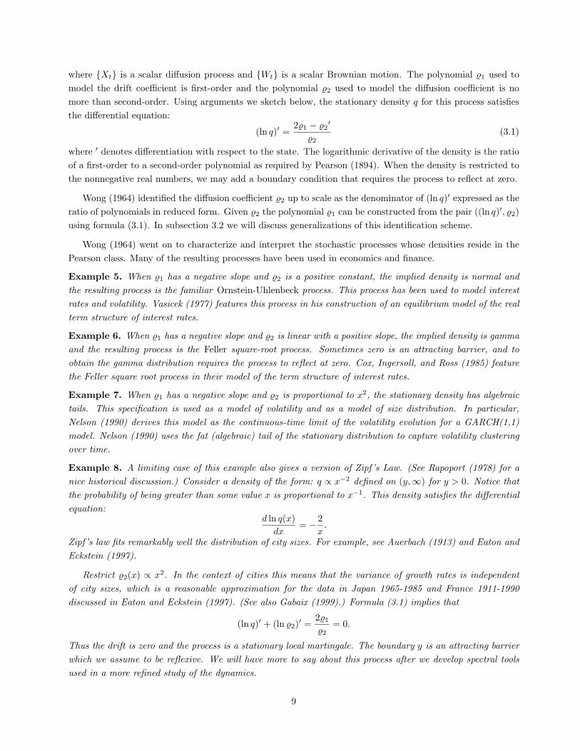
where Xt is a scalar diffusion process and Wt is a scalar Brownian motion. The polynomial %1 used tomodel the drift coefficient is first-order and the polynomial %2 used to model the diffusion coefficient is nomore than second-order. Using arguments we sketch below, the stationary density q for this process satisfiesthe differential equation:

(ln q)′ =2%1 − %2

′

%2(3.1)

where ′ denotes differentiation with respect to the state. The logarithmic derivative of the density is the ratioof a first-order to a second-order polynomial as required by Pearson (1894). When the density is restricted tothe nonnegative real numbers, we may add a boundary condition that requires the process to reflect at zero.

Wong (1964) identified the diffusion coefficient %2 up to scale as the denominator of (ln q)′ expressed as theratio of polynomials in reduced form. Given %2 the polynomial %1 can be constructed from the pair ((ln q)′, %2)using formula (3.1). In subsection 3.2 we will discuss generalizations of this identification scheme.

Wong (1964) went on to characterize and interpret the stochastic processes whose densities reside in thePearson class. Many of the resulting processes have been used in economics and finance.

Example 5. When %1 has a negative slope and %2 is a positive constant, the implied density is normal andthe resulting process is the familiar Ornstein-Uhlenbeck process. This process has been used to model interestrates and volatility. Vasicek (1977) features this process in his construction of an equilibrium model of the realterm structure of interest rates.

Example 6. When %1 has a negative slope and %2 is linear with a positive slope, the implied density is gammaand the resulting process is the Feller square-root process. Sometimes zero is an attracting barrier, and toobtain the gamma distribution requires the process to reflect at zero. Cox, Ingersoll, and Ross (1985) featurethe Feller square root process in their model of the term structure of interest rates.

Example 7. When %1 has a negative slope and %2 is proportional to x2, the stationary density has algebraictails. This specification is used as a model of volatility and as a model of size distribution. In particular,Nelson (1990) derives this model as the continuous-time limit of the volatility evolution for a GARCH(1,1)model. Nelson (1990) uses the fat (algebraic) tail of the stationary distribution to capture volatility clusteringover time.

Example 8. A limiting case of this example also gives a version of Zipf ’s Law. (See Rapoport (1978) for anice historical discussion.) Consider a density of the form: q ∝ x−2 defined on (y,∞) for y > 0. Notice thatthe probability of being greater than some value x is proportional to x−1. This density satisfies the differentialequation:

d ln q(x)dx

= − 2x.

Zipf’s law fits remarkably well the distribution of city sizes. For example, see Auerbach (1913) and Eaton andEckstein (1997).

Restrict %2(x) ∝ x2. In the context of cities this means that the variance of growth rates is independentof city sizes, which is a reasonable approximation for the data in Japan 1965-1985 and France 1911-1990discussed in Eaton and Eckstein (1997). (See also Gabaix (1999).) Formula (3.1) implies that

(ln q)′ + (ln %2)′ =2%1

%2= 0.

Thus the drift is zero and the process is a stationary local martingale. The boundary y is an attracting barrierwhich we assume to be reflexive. We will have more to say about this process after we develop spectral toolsused in a more refined study of the dynamics.

9

The density q ∝ x−2 has a mode at the left boundary y. For the corresponding diffusion model, y is areflecting barrier. Zipf ’s Law is typically a statement about the density for large x, however. Thus we couldlet the left boundary be at zero (instead of y > 0) and set %1 to a positive constant. The implied densitybehaves like a constant multiple of x−2 in the right tail, but the zero boundary will not be attainable. Theresulting density has an interior mode at one-half times the constant value of %1. This density remains withinthe Pearson family.

Example 9. When %1 is a negative constant and %2 is a positive constant, the stationary density is exponentialand the process is a Brownian motion with a negative drift and a reflecting barrier at zero. This process isrelated to the one used to produce Zipf ’s law. Consider the density of the logarithm of x. The Zipf’s Law impliedstationary distribution of lnx is exponential translated by ln y. When the diffusion coefficient is constant, sayα2, the drift of lnx is −α2

2 .

The Wong (1964) analysis is very nice because it provides a rather complete characterization of the tran-sition dynamics of the alternative processes investigated. Subsequently, we will describe some of the spectralor eigenfunction characterizations of dynamic evolution used by Wong (1964) and others. It is the abilityto characterize the transition dynamics fully that has made the processes studied by Wong (1964) valuablebuilding blocks for models in economics and finance. Nevertheless, it is often convenient to move outside thisfamily of models.

Within the Pearson class, (ln q)′ can only have one interior zero. Thus stationary densities must have atmost one interior mode. To build diffusion processes with multi-modal densities, Cobb, Koppstein, and Chan(1983) consider models in which %1 or %2 can be higher-order polynomials. Since Zipf’s Law is arguably abouttail properties of a density, nonlinear drift specifications (specifications of %1) are compatible with this law.Chan, Karolyi, Longstaff, and Sanders (1992) consider models of short-term interest rates in which the driftremains linear, but the diffusion coefficient is some power of x other than linear or quadratic. They treat thevolatility elasticity as a free parameter to be estimated and a focal point of their investigation. Aıt-Sahalia(1996b) compares the constant volatility elasticity model to other volatility specifications, also allowing fora nonlinear drift. Conley, Hansen, Luttmer, and Scheinkman (1997) study the constant volatility elasticitymodel but allowing for drift nonlinearity. Jones (2003) uses constant volatility elasticity models to extendNelson (1990)’s model of the dynamic evolution of volatility.

3.2 Stationary Distributions

To generalize the approach of Wong (1964), we study how to go from the infinitesimal generator to thestationary distribution. Given a generator A of a Feller process, we can deduce an integral equation for thestationary distribution. This formula is given by:

limτ↓0

∫ Tτφ− φτ

dQ =∫AφdQ = 0 (3.2)

for test functions φ in the domain of the generator. (In fact the collection of functions used to check thiscondition can be reduced to a smaller collection of functions called the core of the generator. See Ethier andKurtz (1986) for a discussion.)

Integral equation (3.2) gives rise to the differential equation used by Wong (1964) [see (3.1)] and others.Consider test functions φ that are twice continuously differentiable and have zero derivatives at the boundaries

10

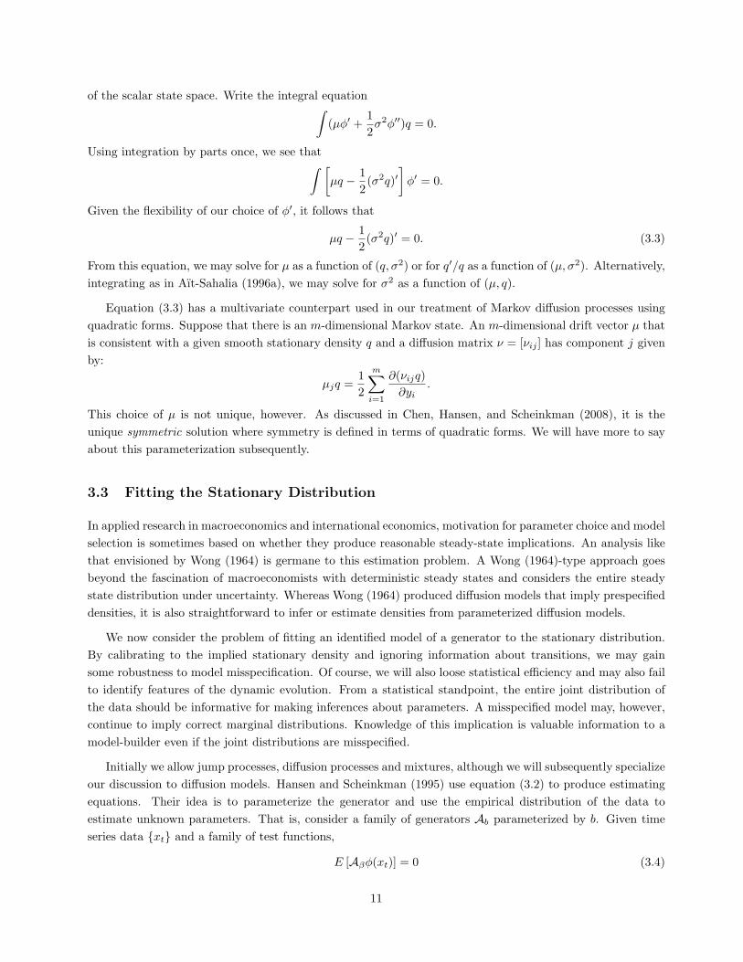
of the scalar state space. Write the integral equation∫(µφ′ +

12σ2φ′′)q = 0.

Using integration by parts once, we see that∫ [µq − 1

2(σ2q)′

]φ′ = 0.

Given the flexibility of our choice of φ′, it follows that

µq − 12

(σ2q)′ = 0. (3.3)

From this equation, we may solve for µ as a function of (q, σ2) or for q′/q as a function of (µ, σ2). Alternatively,integrating as in Aıt-Sahalia (1996a), we may solve for σ2 as a function of (µ, q).

Equation (3.3) has a multivariate counterpart used in our treatment of Markov diffusion processes usingquadratic forms. Suppose that there is an m-dimensional Markov state. An m-dimensional drift vector µ thatis consistent with a given smooth stationary density q and a diffusion matrix ν = [νij ] has component j givenby:

µjq =12

m∑i=1

∂(νijq)∂yi

.

This choice of µ is not unique, however. As discussed in Chen, Hansen, and Scheinkman (2008), it is theunique symmetric solution where symmetry is defined in terms of quadratic forms. We will have more to sayabout this parameterization subsequently.

3.3 Fitting the Stationary Distribution

In applied research in macroeconomics and international economics, motivation for parameter choice and modelselection is sometimes based on whether they produce reasonable steady-state implications. An analysis likethat envisioned by Wong (1964) is germane to this estimation problem. A Wong (1964)-type approach goesbeyond the fascination of macroeconomists with deterministic steady states and considers the entire steadystate distribution under uncertainty. Whereas Wong (1964) produced diffusion models that imply prespecifieddensities, it is also straightforward to infer or estimate densities from parameterized diffusion models.

We now consider the problem of fitting an identified model of a generator to the stationary distribution.By calibrating to the implied stationary density and ignoring information about transitions, we may gainsome robustness to model misspecification. Of course, we will also loose statistical efficiency and may also failto identify features of the dynamic evolution. From a statistical standpoint, the entire joint distribution ofthe data should be informative for making inferences about parameters. A misspecified model may, however,continue to imply correct marginal distributions. Knowledge of this implication is valuable information to amodel-builder even if the joint distributions are misspecified.

Initially we allow jump processes, diffusion processes and mixtures, although we will subsequently specializeour discussion to diffusion models. Hansen and Scheinkman (1995) use equation (3.2) to produce estimatingequations. Their idea is to parameterize the generator and use the empirical distribution of the data toestimate unknown parameters. That is, consider a family of generators Ab parameterized by b. Given timeseries data xt and a family of test functions,

E [Aβφ(xt)] = 0 (3.4)

11

for a finite set of test functions where β is the parameter vector for the Markov model used to generate thedata. This can be posed as a generalized-method-of-moments (GMM) estimation problem of the form studiedby Hansen (1982).

Two questions arise in applying this approach. Can the parameter β in fact be identified? Can suchan estimator be efficient? To answer the first question in the affirmative often requires that we limit theparameterization. We may address Fisher (1921)’s concerns about statistical efficiency by looking over a rich(infinite-dimensional) family of test functions using characterizations provided in Hansen (1985). Even if weassume a finite dimensional parametrization, statistical efficiency is still not attained because this methodignores information on transition densities. Nevertheless, we may consider a more limited notion of efficiencybecause our aim is to fit only the stationary distribution.

In some analyses of Markov process models of stationary densities it is sometimes natural to think of thedata as being draws from independent stochastic processes with the same stationary density. This is the casefor many applications of Zipf’s law. This view is also taken by Cobb, Koppstein, and Chan (1983). We nowconsider the case in which data are obtained from a single stochastic process. The analysis is greatly simplifiedby assuming a continuous-time record of the Markov process between date zero and T . We use a central limitapproximation as the horizon T becomes large. From Bhattacharya (1982) or Hansen and Scheinkman (1995)we know that

1√T

∫ T

0

Aβφ⇒ Normal(0,−2 < Aβφ|φ >) (3.5)

where ⇒ denotes convergence in distribution, and

< Aβφ|φ > .=∫φ (Aβφ) dQ,

for φ in the L2(Q) domain of Aβ . This central limit approximation is a refinement of (3.4) and uses an explicitmartingale approximation. It avoids having to first demonstrate mixing properties.

Using this continuous-time martingale approximation, we may revisit Fisher (1921)’s critique of Pearson(1894). Consider the special case of a scalar stationary diffusion. Fisher (1921) noted that Pearson (1894)’sestimation method was inefficient, because his moment conditions differed from those implicit in maximumlikelihood estimation. Pearson (1894) shunned such methods because they were harder to implement inpractice. Of course computational costs have been dramatically reduced since the time of this discussion.What is interesting is that when the data come from (a finite interval of) a single realization of a scalardiffusion, then the analysis of efficiency is altered. As shown by Conley, Hansen, Luttmer, and Scheinkman(1997), instead of using the score vector for building moment conditions the score vector could be used as testfunctions in relation (3.4).

To use this approach in practice, we need a simple way to compute the requisite derivatives. The scorevector for a scalar parameterization is:

φ =d ln qbdb

(β).

Recall that what enters the moment conditions are test function first and second derivatives (with respect tothe state). That is, we must know φ′ and φ′′, but not φ. Thus we need not ever compute ln q as a function ofb. Instead we may use the formula:

ln qb′ =2µbσ2b

− lnσ2b′

to compute derivatives with respect to the unknown parameters. Even though the score depends on the true

12

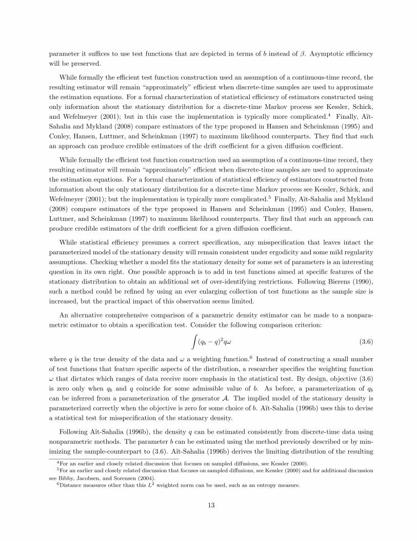
parameter it suffices to use test functions that are depicted in terms of b instead of β. Asymptotic efficiencywill be preserved.

While formally the efficient test function construction used an assumption of a continuous-time record, theresulting estimator will remain “approximately” efficient when discrete-time samples are used to approximatethe estimation equations. For a formal characterization of statistical efficiency of estimators constructed usingonly information about the stationary distribution for a discrete-time Markov process see Kessler, Schick,and Wefelmeyer (2001); but in this case the implementation is typically more complicated.4 Finally, Aıt-Sahalia and Mykland (2008) compare estimators of the type proposed in Hansen and Scheinkman (1995) andConley, Hansen, Luttmer, and Scheinkman (1997) to maximum likelihood counterparts. They find that suchan approach can produce credible estimators of the drift coefficient for a given diffusion coefficient.

While formally the efficient test function construction used an assumption of a continuous-time record, theyresulting estimator will remain “approximately” efficient when discrete-time samples are used to approximatethe estimation equations. For a formal characterization of statistical efficiency of estimators constructed frominformation about the only stationary distribution for a discrete-time Markov process see Kessler, Schick, andWefelmeyer (2001); but the implementation is typically more complicated.5 Finally, Aıt-Sahalia and Mykland(2008) compare estimators of the type proposed in Hansen and Scheinkman (1995) and Conley, Hansen,Luttmer, and Scheinkman (1997) to maximum likelihood counterparts. They find that such an approach canproduce credible estimators of the drift coefficient for a given diffusion coefficient.

While statistical efficiency presumes a correct specification, any misspecification that leaves intact theparameterized model of the stationary density will remain consistent under ergodicity and some mild regularityassumptions. Checking whether a model fits the stationary density for some set of parameters is an interestingquestion in its own right. One possible approach is to add in test functions aimed at specific features of thestationary distribution to obtain an additional set of over-identifying restrictions. Following Bierens (1990),such a method could be refined by using an ever enlarging collection of test functions as the sample size isincreased, but the practical impact of this observation seems limited.

An alternative comprehensive comparison of a parametric density estimator can be made to a nonpara-metric estimator to obtain a specification test. Consider the following comparison criterion:∫

(qb − q)2qω (3.6)

where q is the true density of the data and ω a weighting function.6 Instead of constructing a small numberof test functions that feature specific aspects of the distribution, a researcher specifies the weighting functionω that dictates which ranges of data receive more emphasis in the statistical test. By design, objective (3.6)is zero only when qb and q coincide for some admissible value of b. As before, a parameterization of qbcan be inferred from a parameterization of the generator A. The implied model of the stationary density isparameterized correctly when the objective is zero for some choice of b. Aıt-Sahalia (1996b) uses this to devisea statistical test for misspecification of the stationary density.

Following Aıt-Sahalia (1996b), the density q can be estimated consistently from discrete-time data usingnonparametric methods. The parameter b can be estimated using the method previously described or by min-imizing the sample-counterpart to (3.6). Aıt-Sahalia (1996b) derives the limiting distribution of the resulting

4For an earlier and closely related discussion that focuses on sampled diffusions, see Kessler (2000).5For an earlier and closely related discussion that focuses on sampled diffusions, see Kessler (2000) and for additional discussion

see Bibby, Jacobsen, and Sorensen (2004).6Distance measures other than this L2 weighted norm can be used, such as an entropy measure.

13

test statistic and applies this method to test models of the short-term interest rate process.7 One challengefacing such nonparametric tests is producing accurate small sample distributions. The convergence to theasymptotic distribution obtained by assuming stationarity of the process can be slow when the data are highlypersistent, as is the case with US interest rates. (See Pritsker (1998) and Conley, Hansen, and Liu (1999).)

3.4 Nonparametric Methods for Inferring Drift or Diffusion Coefficients

Recall that for a scalar diffusion, the drift coefficient can be inferred from a stationary density, the diffusioncoefficient and their derivatives. Alternatively the diffusion coefficient can be deduced from the density andthe drift coefficient. These functional relationships give rise to nonparametric estimation methods for the driftcoefficient or the diffusion coefficient. In this subsection we describe how to use local parametrizations of thedrift or the diffusion coefficient to obtain nonparametric estimates. The parameterizations become localizedby their use of test functions or kernels familiar from the literature on nonparametric estimation. The localapproaches for constructing estimators of µ or σ2 estimate nonparametrically one piece (µ or σ2) given anestimate of the other piece.

In the framework of test functions, these estimation methods can be viewed as follows. In the case of ascalar diffusion, ∫

(µφ′ +12σ2φ′′)q = 0. (3.7)

Construct a test function φ such that φ′ is zero everywhere except in the vicinity of some pre-specified pointy. The function φ′ can be thought of as a kernel and its localization can be governed by the choice of abandwidth. As in Banon (1978), suppose that the diffusion coefficient is known. We can construct a locallyconstant estimator of µ that is very close to Banon (1978)’s estimator by solving the sample counterpart to(3.7) under the possibly false assumption that µ is constant. The local specification of φ′ limits the range overwhich constancy of µ is a good approximation, and the method produces a local estimator of µ at the pointy. This method is easily extended to other local parametrizations of the drift. Conley, Hansen, Luttmer, andScheinkman (1997) introduce a local linear estimator by using two local test functions to identify the leveland the slope of the linear approximation. Using logic closely related to that of Florens-Zmirou (1984), theselocal estimators sometimes can presumably be justified when the integrability of q is replaced by a weakerrecurrence assumption.

Suppose that a linear function is in the domain of the generator. Then∫µq = 0. (3.8)

We may now localize the parameterization of the diffusion coefficient by localizing the choice of φ′′. Thespecific construction of φ′ from φ′′ is not essential because moment condition (3.8) is satisfied. For instance,when φ′′ is scaled appropriately to be a density function, we may choose φ′ to be its corresponding distributionfunction. Applying integration by parts to (3.7), we obtain∫ r

l

µ(x)φ′(x)q(x)dx =∫ r

l

[∫ r

x

µq

]φ′′(x)dx

provided that the localization function φ′′ has support in the interior of the state space (l, r). By localizing

7See Section 6.4 and Aıt-Sahalia (1996b) for an analogous test based on transition densities.

14

the parameterization of the diffusion coefficient at x, the limiting version of (3.7) is:∫ r

x

µq +σ2(x)q(x)

2= 0.

Using (3.8), we then obtain the diffusion recovery formula derived in Aıt-Sahalia (1996a).

σ2 (x) =2

q (x)

∫ x

l

µ (u) q (u) du. (3.9)

For a given estimator of µ, an estimator of σ2 can be based directly on recovery formula (3.9) as in Aıt-Sahalia (1996a) or by using a locally constant estimator obtained by solving the sample counterpart to (3.7).Not surprisingly, the two approaches turn out to be very similar.

The local approaches for constructing estimators of µ or σ2 require knowledge of estimates of the otherpiece. Suppose we parameterize µ as in Aıt-Sahalia (1996a) to be affine in the state variable, µ(x) = −κ(x−α),and a linear function is in the domain of the generator, then

A(x− α) = −κ(x− α).

This says that x − α is an eigenfunction of A, with eigenvalue −κ. We shall have more to say about eigen-functions and eigenvalues in section 4. The conditional expectation operator for any interval t must have thesame eigenfunction and an eigenvalue given via the exponential formula:

Ttx = E [Xt|X0] = α+ e−κt (X0 − α) . (3.10)

This conditional moment condition applies for any t > 0. As a consequence, (α, κ) can be recovered by esti-mating a first order scalar autoregression via least squares for data sampled at any interval t = ∆. FollowingAıt-Sahalia (1996a), the implied drift estimator may be plugged into formula (3.9) to produce a semiparame-teric estimator of σ2 (x). Since (3.10) does not require that the time interval be small, this estimator of σ2 (x)can be computed from data sampled at any time interval ∆, not just small ones.

As an alternative, Conley, Hansen, Luttmer, and Scheinkman (1997) produce a semiparameteric estimatorby adopting a constant volatility elasticity specification of the diffusion coefficient, while letting the drift benonparametric. The volatility elasticity is identified by using an additional set of moment conditions derivedin section 6.4 applicable for some subordinated diffusion models. Subordinated Markov processes will bedeveloped in 6.7.

We will have more to say about observable implications including nonparametric identification in section6.

4 Transition Dynamics and Spectral Decomposition

We use quadratic forms and eigenfunctions to produce decompositions of both the stationary distribution andthe dynamic evolution of the process. These decompositions show what features of the time series dominate inthe long run and, more generally, give decompositions of the transient dynamics. While the stationary densitygives one notion of the long run, transition distributions are essential to understanding the full dynamicimplications of nonlinear Markov models. Moreover, stationary distributions are typically not sufficient toidentify all of the parameters of interest. We follow Wong (1964) by characterizing transition dynamics using a

15

spectral decomposition. This decomposition is analogous to the spectral or principal component decompositionof a symmetric matrix. Since we are interested in nonlinear dynamics, we develop a functional counterpart toprincipal component analysis.

4.1 Quadratic Forms and Implied Generators

Previously, we demonstrated that a scalar diffusion can be constructed using a density q and a diffusioncoefficient σ2. By using quadratic forms described in Section 2, we may extend this construction to a broaderclass of Markov process models. The form construction allows us to define a nonlinear version of principalcomponents.

Let Q be a Radon measure on the state space X. For the time being this measure need not be finite,although we will subsequently add this restriction. When Q is finite, after normalization it will be thestationary distribution of the corresponding Markov process. We consider two positive semi-definite quadraticforms on the space of functions L2(Q). One is given by the usual inner product:

f1(φ, ψ) .=< φ,ψ >=∫φψdQ.

This form is symmetric [f1(φ, ψ) = f1(ψ, φ)] and positive semidefinite (f1(φ, φ) ≥ 0).

The second form is constructed from two objects: (a) a state dependent positive semidefinite matrixν and (b) a symmetric, positive Radon measure R on the product space X × X excluding the diagonalD

.= (x, x) : x ∈ X with ∫X×X−D

|x− y|21 + |x− y|2R(dx, dy) <∞.

It is given by:

f2(φ, ψ) .=12

∫(∇φ)∗ν(∇ψ)dQ+

12

∫[φ(y)− φ(x)][ψ(y)− ψ(x)]R(dx, dy)

where ∗ is used to denote transposition.8 The form f2 is well-defined at least on the space C2K of twice

continuously differentiable functions with compact support. Under additional regularity conditions, the formf2 is closable, that is, it has a closed extension in L2(Q).9 However, even this extension has a limited domain.Like f1, the form f2 is also symmetric and positive semidefinite. Notice that f2 is the sum of two forms. Aswe will see, the first is associated with a diffusion process and the second with a jump process.10

4.1.1 Implied Generator

We may now follow the approach of Beurling and Deny (1958) and Fukushima (1971) by constructing a Markovprocess associated with the form f1 and the closed extension of f2. In what follows we will sketch only partof this construction. We describe how to go from the forms f1 and f2 to an implied generator. The generatorA is the symmetric solution to:

f2(φ, ψ) = −f1[(Aφ), ψ] = −∫

(Aφ)ψdQ. (4.1)

8We may use weak gradients in the construction of f2.9For instance if Q has density q, and q and ν are continuously differentiable, then the form f2 is closable.

10In fact there exist generalizations of this representation in which ν is replaced by a matrix-valued measure and an additional

term∫φ(x)ψ(x)dk(x) is introduced where k is a killing measure. See Beurling and Deny (1958) and Fukushima, Oshima, and

Takeda (1994).

16

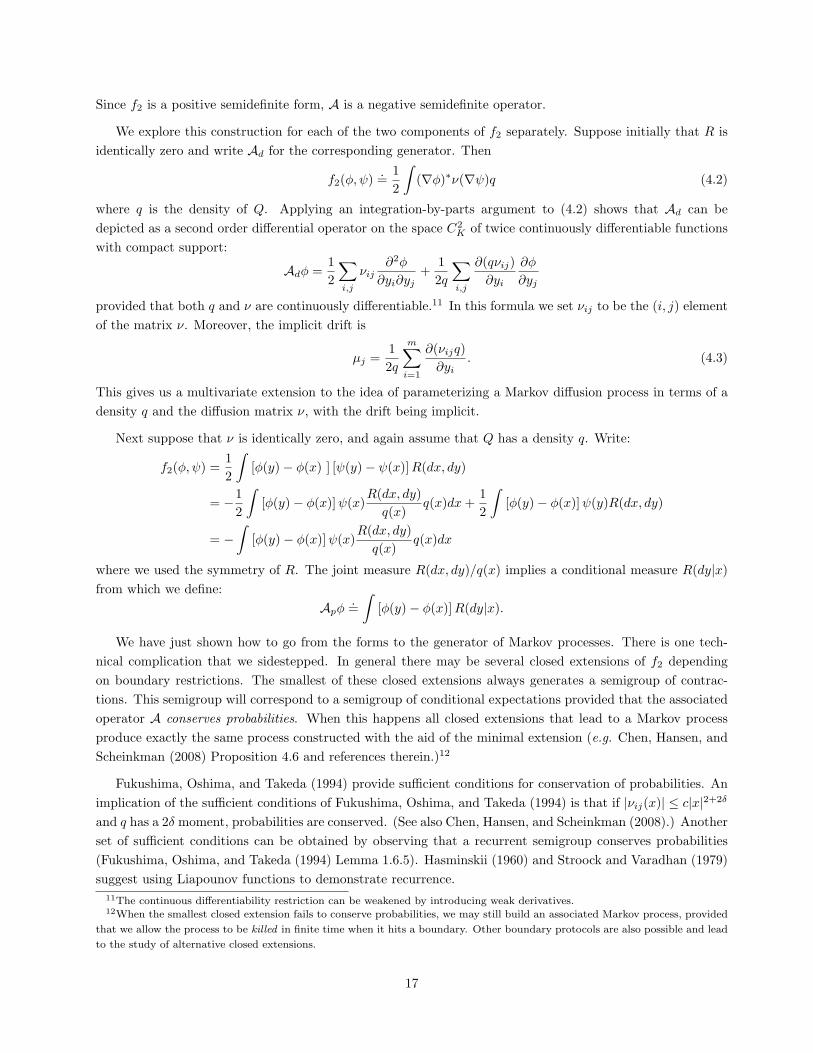
Since f2 is a positive semidefinite form, A is a negative semidefinite operator.

We explore this construction for each of the two components of f2 separately. Suppose initially that R isidentically zero and write Ad for the corresponding generator. Then

f2(φ, ψ) .=12

∫(∇φ)∗ν(∇ψ)q (4.2)

where q is the density of Q. Applying an integration-by-parts argument to (4.2) shows that Ad can bedepicted as a second order differential operator on the space C2

K of twice continuously differentiable functionswith compact support:

Adφ =12

∑i,j

νij∂2φ

∂yi∂yj+

12q

∑i,j

∂(qνij)∂yi

∂φ

∂yj

provided that both q and ν are continuously differentiable.11 In this formula we set νij to be the (i, j) elementof the matrix ν. Moreover, the implicit drift is

µj =12q

m∑i=1

∂(νijq)∂yi

. (4.3)

This gives us a multivariate extension to the idea of parameterizing a Markov diffusion process in terms of adensity q and the diffusion matrix ν, with the drift being implicit.

Next suppose that ν is identically zero, and again assume that Q has a density q. Write:

f2(φ, ψ) =12

∫[φ(y)− φ(x) ] [ψ(y)− ψ(x)]R(dx, dy)

= −12

∫[φ(y)− φ(x)]ψ(x)

R(dx, dy)q(x)

q(x)dx+12

∫[φ(y)− φ(x)]ψ(y)R(dx, dy)

= −∫

[φ(y)− φ(x)]ψ(x)R(dx, dy)q(x)

q(x)dx

where we used the symmetry of R. The joint measure R(dx, dy)/q(x) implies a conditional measure R(dy|x)from which we define:

Apφ .=∫

[φ(y)− φ(x)]R(dy|x).

We have just shown how to go from the forms to the generator of Markov processes. There is one tech-nical complication that we sidestepped. In general there may be several closed extensions of f2 dependingon boundary restrictions. The smallest of these closed extensions always generates a semigroup of contrac-tions. This semigroup will correspond to a semigroup of conditional expectations provided that the associatedoperator A conserves probabilities. When this happens all closed extensions that lead to a Markov processproduce exactly the same process constructed with the aid of the minimal extension (e.g. Chen, Hansen, andScheinkman (2008) Proposition 4.6 and references therein.)12

Fukushima, Oshima, and Takeda (1994) provide sufficient conditions for conservation of probabilities. Animplication of the sufficient conditions of Fukushima, Oshima, and Takeda (1994) is that if |νij(x)| ≤ c|x|2+2δ

and q has a 2δ moment, probabilities are conserved. (See also Chen, Hansen, and Scheinkman (2008).) Anotherset of sufficient conditions can be obtained by observing that a recurrent semigroup conserves probabilities(Fukushima, Oshima, and Takeda (1994) Lemma 1.6.5). Hasminskii (1960) and Stroock and Varadhan (1979)suggest using Liapounov functions to demonstrate recurrence.

11The continuous differentiability restriction can be weakened by introducing weak derivatives.12When the smallest closed extension fails to conserve probabilities, we may still build an associated Markov process, provided

that we allow the process to be killed in finite time when it hits a boundary. Other boundary protocols are also possible and lead

to the study of alternative closed extensions.

17

4.1.2 Symmetrization

There are typically nonsymmetric solutions to (4.1). Given a generator A, let A∗ denote its adjoint. Define asymmetrized generator as:

As =A+A∗

2.

Then As can be recovered from the forms f1 and f2 using the algorithm suggested previously. The symmetrizedversion of the generator is identified by the forms, while the generator itself is not.

We consider a third form using one-half the difference between A and A∗. Define:

f3(φ, ψ) =∫ (A−A∗

2φ

)ψdQ.

This form is clearly anti-symmetric. That is

f3(φ, ψ) = −f3(ψ, φ)

for all φ and ψ in the common domain of A and its adjoint. We may recover a version of A+A∗2 from (f1, f2)

and A−A∗

2 from (f1, f3). Taken together we may construct A. Thus to study nonsymmetric Markov processesvia forms, we are led to introduce a third form, which is antisymmetric. See Ma and Rockner (1991) for anexposition of nonsymmetric forms and their resulting semigroups.

In what follows we specialize our discussion to the case of multivariate diffusions. When the dimensionof the state space is greater than one, there are typically also nonsymmetric solutions to (4.1). Forms donot determine uniquely operators without additional restrictions such as symmetry. These nonsymmetricsolutions are also generators of diffusion processes. While the diffusion matrix is the same for the operatorand its adjoint, the drift vectors differ. Let µ denote the drift for a possibly nonsymmetric solution, µs

denote the drift for the symmetric solution given by (4.3), and let µ∗ denote the drift for the adjoint of thenonsymmetric solution. Then

µs =µ∗ + µ

2.

The form pair (f1, f2) identifies µs but not necessarily µ.

The form f3 can be depicted as:

f3(φ, ψ) =12

∫[(µ− µ∗) · (∇φ)]ψq

at least for functions that are twice continuously differentiable and have compact support. For such functionswe may use integration by parts to show that in fact:

f3(φ, ψ) = −f3(ψ, φ).

Moreover, when q is a density, we may extend f3 to include constant functions via

f3(φ, 1) =12

∫(µ− µ∗) · (∇φ)q = 0.

4.2 Principal Components

Given two quadratic forms, we define the functional versions of principal components.

18

Definition 6. Nonlinear principal components are functions ψj , j = 1, 2 . . . that solve:

maxφ

f1(φ, φ)

subject to

f2(φ, φ) = 1

f1(φ, ψs) = 0, s = 0, ..., j − 1

where ψ0 is initialized to be the constant function one.

This definition follows Chen, Hansen, and Scheinkman (2008) and is a direct extension of that used bySalinelli (1998) for iid data. In the case of a diffusion specification, form f2 is given by (4.2) and induces aquadratic smoothness penalty. Principal components maximize variation subject to a smoothness constraintand orthogonality. These components are a nonlinear counterpart to the more familiar principal componentanalysis of covariance matrices advocated by Pearson (1901). In the functional version, the state dependent,positive definite matrix ν is used to measure smoothness. Salinelli (1998) advocated this version of principalcomponent analysis for ν = I to summarize the properties of i.i.d. data. As argued by Chen, Hansen, andScheinkman (2008) they are equally valuable in the analysis of time series data. The principal components,when they exist, will be orthogonal under either form. That is:

f1(ψj , ψk) = f2(ψj , ψk) = 0

provided that j 6= k.

These principal components coincide with the principal components from the canonical analysis used byDarolles, Florens, and Gourieroux (2000) under symmetry, but otherwise they differ. In addition to maximizingvariation under smoothness restrictions (subject to orthogonality), they maximize autocorrelation and theymaximize the long run variance as measured by the spectral density at frequency zero. See Chen, Hansen,and Scheinkman (2008) for an elaboration.

This form approach and the resulting principal component construction is equally applicable to i.i.d. dataand to time series data. In the i.i.d. case, the matrix ν is used to measure function smoothness. Of coursein the i.i.d. case there is no connection between the properties of ν and the data generator. The Markovdiffusion model provides this link.

The smoothness penalty is special to diffusion processes. For jump processes, the form f2 is built using themeasure R, which still can be used to define principal components. These principal components will continueto maximize autocorrelation and long run variance subject to orthogonality constraints.

4.2.1 Existence

It turns out that principal components do not always exist. Existence is straightforward when the state spaceis compact, the density q is bounded above and bounded away from zero and the diffusion matrix is uniformlynonsingular on the state space. These restrictions are too severe for many applications. Chen, Hansen, andScheinkman (2008) treat cases where these conditions fail.

Suppose the state space is not compact. When the density q has thin tails, the notion of approximationis weaker. Approximation errors are permitted to be larger in the tails. This turns out to be one mechanism

19

for the existence of principal components. Alternatively, ν might increase in the tails of the distribution of qlimiting the admissible functions. This can also be exploited to establish the existence of principal components.

Chen, Hansen, and Scheinkman (2008) exhibit sufficient conditions for existence that require a trade-offbetween growth in ν and tail thinness of the density q. Consider the (lower) radial bounds,

ν(x) ≥ c(1 + |x|2)βI

q(x) ≥ exp[−2ϑ(|x|)].

Principal components exist when 0 ≤ β ≤ 1 and rβϑ′(r)→∞ as r gets large. Similarly, they also exist whenϑ(r) = γ

2 ln(1 + r2) + c∗, and 1 < β < γ − m2 + 1. The first set of sufficient conditions is applicable when the

density q has an exponentially thin tail; the second is useful when q has an algebraic tail.

We now consider some special results for the case m = 1. We let the state space be (l, r), where eitherboundary can be infinite. Again q denotes the stationary density and σ > 0 the volatility coefficient (that is,σ2 = ν.) Suppose that ∫ r

l

∣∣∣∣∫ x

xo

1q(y)σ2(y)

dy

∣∣∣∣ q(x)dx <∞ (4.4)

where xo is an interior point in the state space. Then principal components are known to exist. For a proofsee, e.g. Hansen, Scheinkman, and Touzi (1998), page 13, where this proposition is stated using the scalefunction

s(x) .=∫ x

xo

1q(y)σ2(y)

dy,

and it is observed that (4.4) admits entrance boundaries, in addition to attracting boundaries.

When assumption (4.4) is not satisfied, at least one of the boundaries is natural. Recall that the boundaryl (r) is natural if s(l) = −∞ (s(r) = +∞ resp.) and,∫ x0

l

s(x)q(x)dx = −∞(∫ r

x0

s(x)q(x)dx = +∞ resp.)

Hansen, Scheinkman, and Touzi (1998) show that in this case principal components exist whenever

lim supx→r

µ

σ− σ′

2= lim sup

x→r

σq′

2q+σ′

2= −∞

lim infx→l

µ

σ− σ′

2= lim inf

x→lσq′

2q+σ′

2= +∞. (4.5)

We can think of the left-hand side of (4.5) as a local measure of pull towards the center of the distribution. Ifone boundary, say l, is reflexive and r is natural, then a principal component decomposition exists providedthat the lim inf in (4.5) is +∞.

4.2.2 Spectral Decomposition

Principal components, when they exist, can be used to construct the semigroup of conditional expectation op-erators as in Wong (1964). A principal component decomposition is analogous to the spectral decomposition ofa symmetric matrix. Each principal component is an eigenfunction of all of the conditional expectation opera-tors and hence behaves like a first-order scalar autoregression (with conditionally heteroskedastic innovations).See Darolles, Florens, and Gourieroux (2001) for an elaboration. Thus principal components constructed fromthe stationary distribution must satisfy an extensive family of conditional moment restrictions.

20

Both the generator and the semigroup of conditional expectations operators have spectral (principal com-ponent) decompositions. The generator has spectral decomposition:

Aφ =∞∑j=0

−δjf1(ψj , φ)ψj ,

where each δj > 0 and, ψj is a principal component (normalized to have a unit second moment) and aneigenvector associated with the eigenvalue −δj , that is,

Aψj = −δjψj .

The corresponding decomposition for the semigroup uses an exponential formula:

T∆φ =∞∑j=0

exp(−∆δj)f1(ψj , φ)ψj . (4.6)

This spectral decomposition shows that the principal components of the semigroup are ordered in importanceby which dominate in the long run.

Associated with (4.6) for a diffusion is an expansion of the transition density. Write:

p(y|x, t) =∞∑j=0

exp(−tδj)ψj(y)ψj(x)q(y) (4.7)

where q is the stationary density. Notice that we have constructed p(y|x, t) so that

Ttφ(x) =∫φ(y)p(y|x, t)dy.

The basis functions used in this density expansion depend on the underlying model. Recall that an Ornstein-Uhlenbeck process has a stationary distribution that is normal (see Example 5). Decomposition (4.6) is aHermite expansion when the stationary distribution has mean zero and variance one. The eigenfunctions arethe orthonormal polynomials with respect to a standard normal distribution.

4.2.3 Dependence

Spectral decomposition does not require the existence of principal components. We have seen how to con-struct Markov processes with self adjoint generators using forms. A more general version of the spectraldecomposition of generators is applicable to the resulting semigroup and generator that generalizes formula(4.6), see Rudin (1973), Hansen and Scheinkman (1995) and Schaumburg (2005). This decomposition is ap-plicable generally for scalar diffusions even when a stationary density fails to exist, for a wide class of Markovprocesses defined via symmetric forms. The measure q used in constructing the forms and defining a sense ofapproximation need not be integrable.

The existence of a principal component decomposition typically requires that the underlying Markov pro-cess be only weakly dependent. For a weakly dependent process, autocorrelations of test functions decayexponentially. It is possible, however, to build models of Markov processes that are strongly dependent. Forsuch processes, the autocorrelations of some test functions decay at a slower than exponential rate. Operatormethods give a convenient way to characterize when a process is strongly dependent.

21

In our study of strongly dependent, but stationary, Markov processes, we follow Chen, Hansen, and Car-rasco (2008) by using two measures of mixing. Both of these measures have been used extensively in thestochastic process literature. The first measure, ρ−mixing uses the L2(Q) formulation. Let

U.= φ ∈ L2(Q) :

∫φdQ = 0,

∫φ2dQ = 1.

The concept of ρ−mixing studies the maximal correlation of two functions of the Markov state in differenttime periods.

Definition 7. The ρ−mixing coefficients of a Markov process are given by:

ρt = supψ,φ∈U

∫ψ (Ttφ) dQ.

The process Xt is ρ−mixing or weakly dependent if limt→∞ ρt = 0.

When the ρ−mixing coefficients of a Markov process decline to zero, they do so exponentially. When aMarkov process has a principal component decomposition, it is ρ−mixing with exponential decay. In fact,ρ−mixing requires something weaker.

As argued by Banon (1978) and Hansen and Scheinkman (1995), ρ−mixing is guaranteed by a gap in thespectrum of the negative semidefinite operator A to the left of zero. Although not always symmetric, theoperator A is negative semidefinite: ∫

φ(Aφ)dQ ≤ 0

on the L2(Q) domain of A. This negative-semidefinite property follows from the restriction that Tt is a weakcontraction on L2(Q) for each t. A spectral gap is present when we can strengthen this restriction as follows:

supφ∈U ⋂D(A)

< φ,Aφ > < 0. (4.8)

When this condition is satisfied Tt is a strong contraction on the subspace U for each t, and the ρ−mixingcoefficients decay exponentially.

In the case of a scalar diffusion, Hansen and Scheinkman (1995) show that this inequality is satisfiedprovided that

lim supx→r

µ

σ− σ′

2= lim sup

x→r

σq′

2q+σ′

2< 0

lim infx→`

µ

σ− σ′

2= lim inf

x→`σq′

2q+σ′

2> 0. (4.9)

where r is the right boundary and ` is the left boundary of the state space. This restriction is a weakeningof restriction (4.5), which guaranteed the existence of principal components. Condition (4.9) guarantees thatthere is sufficient pull from each boundary towards the center of the distribution to imply ρ−mixing. Whenone of these two limits is zero, the ρ−mixing coefficients may be identically equal to one. In this case theMarkov process is strongly dependent.13

Since the ρ−mixing coefficients for a Markov process either decay exponentially or are equal to one, weneed a different notion of mixing to obtain a more refined analysis of strong dependence. This leads us toconsider the β−mixing coefficients:

13Recall that the term in the left-hand side of (4.9) can be interpreted as the drift of a corresponding diffusion with a unit

diffusion coefficient obtained by transforming the scale. As a consequence, condition (4.9) can also be related to Veretennikov

(1997)’s drift restriction for a diffusion to be strongly dependent.

22

Definition 8. The β−mixing coefficients for a Markov process are given by:

βt =∫

sup0≤φ≤1

|Ttφ−∫φdQ|dQ.

The process Xt is β−mixing if limt→∞ βt = 0; is β−mixing with an exponential decay rate if βt ≤ γ exp(−δt)for some δ, γ > 0.

At least for scalar diffusions, Chen, Hansen, and Carrasco (2008) show that the exponential decay of theρ−mixing coefficients is essentially equivalent to the exponential decay of the β−mixing coefficients. Whenthe ρ−mixing coefficients are identically one, however, the β−mixing coefficients will still decay to zero, butat a rate slower than exponential. Thus the decay properties of the β−mixing coefficients provides a moresensitive characterization of strong dependence.

4.3 Applications

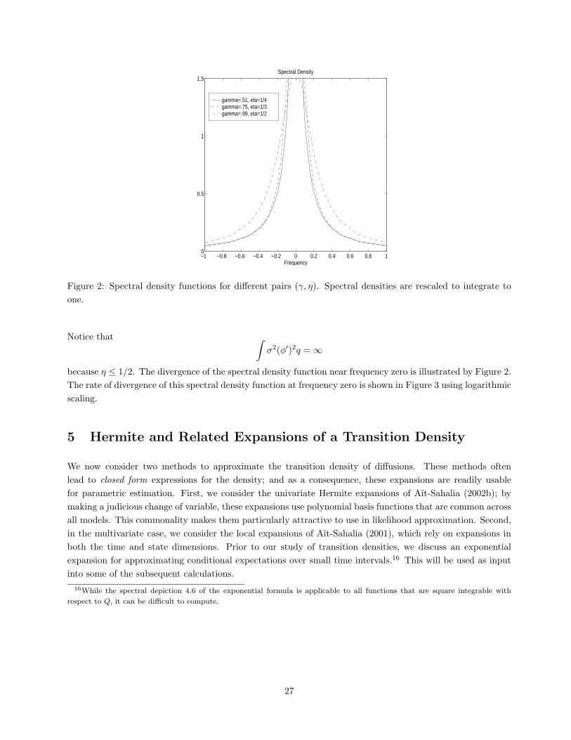
4.3.1 Zipf’s Law

Recall Zipf’s Law discussed in Section 3.1. Zipf suggested a generalization of his law in which there wasa free parameter that related rank to size. Consider a family of stationary densities that satisfy a powerlaw of the form: qξ ∝ x−(2+ξ) defined on (y,∞) where y > 0 and ξ ≥ 0. Then the rank-size relationbecomes size(rank)

11+ξ = constant. This family of densities is of interest to economists, because of power-law

distributions that seem to describe income distribution and city sizes. With σ2(x) = α2x2, the correspondingdrift is, using equation (3.3),

µ = −ξα2x

2Notice that µ(y) < 0, so that y > 0 is an attainable boundary. We make this barrier reflexive to deliver therequisite stationary density.

To study temporal dependence, we consider the pull measure:

µ

σ− σ′

2= −α(1 + ξ)

2,

which is negative and independent of the state. The negative pull at the right boundary in conjunction withthe reflexive left boundary guarantees that the process has a spectral gap and thus it is weakly dependenteven in the case where ξ = 0. Since the pull measure is constant, it fails to satisfy restriction (4.5). The fullprincipal component decomposition we described in section 4.2 fails to exists because the boundary pull isinsufficient.

4.3.2 Stationarity and Volatility

Nonlinearity in a Markov diffusion coefficient changes the appropriate notion of mean reversion. Stationaritycan be induced by how volatility changes as a function of the Markov state and may have little to do with theusual notion of mean reversion as measured by the drift of the diffusion process. This phenomenon is mostdirectly seen in scalar diffusion models in which the drift is zero, but the process itself is stationary. Conley,Hansen, Luttmer, and Scheinkman (1997) generalize this notion by arguing that for stationary processes with

23

an infinite right boundary, the stationarity is volatility induced when:∫ ∞x

µ(y)σ2(y)

dy > −∞ (4.10)

for some x in the interior of the state space. This requirement is sufficient for +∞ not to be attracting. Forthe process to be stationary the diffusion coefficient must grow sufficiently fast as a function of the state.In effect 1/σ2 needs to be integrable. The high volatility in large states is enough to guarantee that theprocess eventually escapes from those states. Reversion to the center of the distribution is induced by thishigh volatility and not by the pull from the drift. An example is Zipf’s with drift µ = 0. Conley, Hansen,Luttmer, and Scheinkman (1997) give examples for models with a constant volatility elasticity.

Jones (2003) uses a stochastic volatility model of equity in which the volatility of volatility ensures thatthe volatility process is stationary. Consider a process for volatility that has a linear drift µ(x) = α− κx andconstant volatility elasticity: σ2(x) ∝ x2γ . Jones estimates that κ is essentially zero for data he considers onequity volatility. Even with a zero value of κ the pull measure µ/σ−σ′/2 diverges to −∞ at the right boundaryprovided that γ is greater than one. Jones (2003) in fact estimates a value for γ that exceeds one. The pullmeasure also diverges at the left boundary to +∞. The process is ρ-mixing and it has a simple spectraldecomposition. Stationarity is volatility induced when κ = 0 because relation (4.10) is satisfied provided thatγ exceeds one. The state-dependence in the volatility (of volatility) is sufficient to pull the process to thecenter of its distribution even though the pull coming from the drift alone is in the wrong direction at theright boundary.

Using parameter estimates from Jones (2003), we display the first five principal components for the volatilityprocess in Figure 1. For the principal component extraction, we use the two weighting functions describedpreviously. For the quadratic form in function levels we weight by the stationary density implied by theseparameter values. The quadratic form in the derivatives is weighted by the stationary density times thediffusion coefficient. As can be see from Figure 1, this function converges to a constant in the right tail of thestationary distribution.

While they are nonlinear, the principal components evaluated at the underlying stochastic process eachbehave like a scalar autoregression with heteroskedastic innovations. As expected the higher-order principalcomponents oscillate more as measured by zero crossings.14 The higher-order principal components are lesssmooth as measured by the quadratic form in the derivatives. Given the weighting used in the quadratic formfor the derivatives, the principal components are flat in the tails.

4.3.3 Approximating Variance Processes

Meddahi (2001) and Andersen, Bollerslev, and Meddahi (2004) use a nonlinear principal component de-composition to study models of volatility. Recall that each principal component behaves as a univariate(heteroskedastic) autoregression and the components are mutually orthogonal. These features of principalcomponents make them attractive for forecasting conditional variances and time-averages of conditional vari-ances. Simple formulas exist for predicting the time-average of a univariate autoregression and Andersen,Bollerslev, and Meddahi (2004) are able apply those formulas in conjunction with a finite number of the mostimportant principal components to obtain operational prediction formulas.

14Formally, the as expected comment comes from the Sturm-Liouville theory of second-order differential equations.

24

0 0.5 1 1.5

x 10−3

−5

0

5

10PC1

0 0.5 1 1.5

x 10−3

−5

0

5

10PC2

0 0.5 1 1.5

x 10−3

−5

0

5

10PC3

0 0.5 1 1.5

x 10−3

−5

0

5

10PC4

0 0.5 1 1.5

x 10−3

−5

0

5

10PC5

0 0.5 1 1.5

x 10−3

0

0.2

0.4

0.6

0.8

1

Weighting functions

Figure 1: The first five principal components for a volatility model estimated by Jones. The weightingfunctions are the density and the density scaled by the diffusion coefficient. The parameter values are κ = 0,α = .58× 10−6, and σ2 = 6.1252x2.66. Except for κ, the parameter values are taken from the fourth column ofTable 1 in Jones. Although the posterior mean for κ is different from zero, it is small relative to its posteriorstandard deviation.

While they are nonlinear, the principal components evaluated at the underlying stochastic process eachbehave like a scalar autoregression with heteroskedastic innovations. As expected the higher-order principalcomponents oscillate more as measured by zero crossings.11 The higher-order principal components are lesssmooth as measured by the quadratic form in the derivatives. Given the weighting used in the quadratic formfor the derivatives, the principal components are flat in the tails.

4.9.3 Approximating Variance Processes

Meddahi (2001) and Andersen, Bollerslev, and Meddahi (2004) use a nonlinear principal component de-composition to study models of volatility. Recall that each principal component behaves as a univariate(heteroskedastic) autoregression and the components are mutually orthogonal. These features of principalcomponents make them attractive for forecasting conditional variances and time-averages of conditional vari-ances. Simple formulas exist for predicting the time-average of a univariate autoregression and Andersen,Bollerslev, and Meddahi (2004) are able apply those formulas in conjunction with a finite number of the mostimportant principal components to obtain operational prediction formulas.

4.9.4 Pricing

As an alternative application, Darolles and Laurent (2000) use a principal component decomposition for scalardiffusions to approximate asset payoffs and prices under a risk neutral probability distribution. Limiting

11Formally, the as expected comment comes from the Sturm-Luiville theory of second-order differential equations.

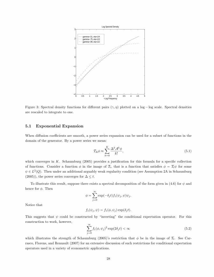
25

Figure 1: The first five principal components for a volatility model estimated by Jones. The weightingfunctions are the density and the density scaled by the diffusion coefficient. The parameter values are κ = 0,α = .58× 10−6, and σ2 = 6.1252x2.66. Except for κ, the parameter values are taken from the fourth column ofTable 1 in Jones. Although the posterior mean for κ is different from zero, it is small relative to its posteriorstandard deviation.

25

4.3.4 Imitating Long Memory Processes

Linear characterizations of time series typically define long memory in terms of the behavior of the spectraldensity function (the Fourier transform of the autocovariance function). When the spectral density divergesto infinity at zero, there is strong linear dependence. The degree of fractional integration is defined using therate at which this spectral density diverges. As we have seen, stationary Markov processes can be stronglydependent as characterized by the behavior of the implied mixing coefficients.

The spectral density function at frequency zero is typically the variance used in a central limit approxi-mation. From Bhattacharya (1982) and Hansen and Scheinkman (1995) and formula (3.5), we know that theasymptotic variance for the central limit approximation for 1√

T

∫ T0Aφ(xt) is:

2f2(φ, φ) = −2∫φ(Aφ)dQ =

∫(∇φ)∗ν(∇φ)q

where the second right-hand side expression is the formula for diffusion processes. The formula for jumpprocesses is different. Thus the long-run variance for the process Aφ(xt) is given by the form 2f2 appliedto the test function φ. This long-run variance is also the spectral density at frequency zero.

This long-run variance is not always finite, however. Using this long-run variance, we may define weakdependence as:

supφ∈D(A),

∫A(φ)2dQ=1

f2(φ, φ) <∞.

This is in effect the inverse counterpart to (4.8), and is equivalent to the restriction that the ρ−mixingcoefficients have exponential decay. This criterion also suggests how we might construct strongly dependentdiffusion processes with a divergent spectral density. Find a pair (ν,Q) and a test function φ such that for

ψ.= µ · ∂φ

∂x+

12

trace(ν∂2φ

∂x∂x′

)we have

∫|ψ|2q <∞;

∫ψq = 0; and

∫ (∂φ∂x

)∗ν(∂φ∂x

)=∞.

Such a process gives an alternative way to produce long range dependence to the self similar fractionalBrownian motion model of Mandelbrot and Ness (1968). While these diffusions are not self-similar, they havethe mathematical advantage of being semimartingales.

We illustrate a family of scalar diffusion models that are strongly dependent. It is often argued thatstrong dependence is a feature of volatility models. One important source of evidence for strong dependenceis a spectral density matrix that diverges at frequency zero. We now display one construction of a nonlineardiffusion model that is strongly dependent. This example is taken from Chen, Hansen, and Carrasco (2008).

Consider a scalar process with a zero mean and a diffusion coefficient σ2(x) = (1 + x2)γ for 1/2 < γ < 1.The candidate stationary density is proportional to 1/σ2. In fact this process is stationary, but its ρ−mixingcoefficients are unity. In particular, the pull measure is zero at both boundaries. Form a new process by takinga time invariant transformation of the original process. That is, let

ψ =σ2

2φ′′

where φ is such that φ′(x) = (1 + x2)−η/2. Restrict η to satisfy: γ − 1/2 ≤ η ≤ 1/2. Then ψ has mean zeroand finite variance when integrated against the stationary density.15 Its long run variance, however, is infinite.

15The function φ will not typically be in the L2(Q) domain of the generator.

26

gamma=.51, eta=1/4gamma=.75, eta=1/3gamma=.99, eta=1/2

−1 −0.8 −0.6 −0.4 −0.2 0 0.2 0.4 0.6 0.8 10

0.5

1

1.5

Frequency

Spectral Density

Figure 2: Spectral density functions for different pairs (γ, η). Spectral densities are rescaled to integrate toone.

Notice that ∫σ2(φ′)2q =∞

because η ≤ 1/2. The divergence of the spectral density function near frequency zero is illustrated by Figure 2.The rate of divergence of this spectral density function at frequency zero is shown in Figure 3 using logarithmicscaling.

5 Hermite and Related Expansions of a Transition Density

We now consider two methods to approximate the transition density of diffusions. These methods oftenlead to closed form expressions for the density; and as a consequence, these expansions are readily usablefor parametric estimation. First, we consider the univariate Hermite expansions of Aıt-Sahalia (2002b); bymaking a judicious change of variable, these expansions use polynomial basis functions that are common acrossall models. This commonality makes them particularly attractive to use in likelihood approximation. Second,in the multivariate case, we consider the local expansions of Aıt-Sahalia (2001), which rely on expansions inboth the time and state dimensions. Prior to our study of transition densities, we discuss an exponentialexpansion for approximating conditional expectations over small time intervals.16 This will be used as inputinto some of the subsequent calculations.

16While the spectral depiction 4.6 of the exponential formula is applicable to all functions that are square integrable with

respect to Q, it can be difficult to compute.

27

gamma=.51, eta=1/4gamma=.75, eta=1/3gamma=.99, eta=1/2

0 0.5 1 1.5 2 2.5 3 3.5 4 4.5 5−4

−3

−2

−1

0

1

2

3

−Log Frequency

Log Spectral Density

Figure 3: Spectral density functions for different pairs (γ, η) plotted on a log− log scale. Spectral densitiesare rescaled to integrate to one.

5.1 Exponential Expansion

When diffusion coefficients are smooth, a power series expansion can be used for a subset of functions in thedomain of the generator. By a power series we mean:

T∆φ ≈K∑k=0

∆kAkφk!

, (5.1)

which converges in K. Schaumburg (2005) provides a justification for this formula for a specific collectionof functions. Consider a function φ in the image of Tt, that is a function that satisfies φ = Ttψ for someψ ∈ L2(Q). Then under an additional arguably weak regularity condition (see Assumption 2A in Schaumburg(2005)), the power series converges for ∆ ≤ t.

To illustrate this result, suppose there exists a spectral decomposition of the form given in (4.6) for ψ andhence for φ. Then

φ =∞∑j=0

exp(−δjt)f1(ψj , ψ)ψj .

Notice thatf1(ψj , ψ) = f1(φ, ψj) exp(δjt).

This suggests that ψ could be constructed by “inverting” the conditional expectation operator. For thisconstruction to work, however,

∞∑j=0

f1(φ, ψj)2 exp(2δjt) <∞ (5.2)

which illustrates the strength of Schaumburg (2005)’s restriction that φ be in the image of Tt. See Car-rasco, Florens, and Renuault (2007) for an extensive discussion of such restrictions for conditional expectationoperators used in a variety of econometric applications.

28

When restriction (5.2) is satisfied, we can establish the approximation. Write

K∑k=0

∆kAkφk!

− exp (A)φ =∞∑j=0

[K∑k=0

(−∆δk)k

k!− exp (−∆δj)

]f1(ψj , φ)ψj

=∞∑j=0

[K∑k=0

(−∆δk)k

k!− exp (−∆δj)

]exp(−δjt)f1(ψj , ψ)ψj

The discounting of the coefficients f1(ψk, ψ) by exp(−δkt) is used to limit the magnitude of the approximationerror. Notice that

exp(−tδj)∣∣∣∣∣K∑k=0

(−∆δj)k

k!− exp (−∆δj)

∣∣∣∣∣ ≤ exp(−∆δj)

[K∑k=0

(∆δj)k

k!+ exp(−∆δj)

]≤ 2.

This bound together with the pointwise (in ∆δk) of the power series expansion of the exponential can be usedin conjunction with the Dominated Convergence Theorem to show that the approximation error converges tozero in the norm on L2(Q).

Schaumburg (2005) establishes this approximation without requiring the simple spectral decompositionwe used here. The remaining challenge in using this approach is to characterize more explicitly the set offunctions that are in the image of Tt. For instance, in Wong (1964)’s models with polynomial eigenfunctions,it can be shown that polynomials are in the image of Tt, but it remains an interesting challenge to establishthis property for more general classes of diffusion models.

Kessler (1997) and Stanton (1997) suggest using this expansion method to construct conditional momentrestrictions to be used estimation. In what follows we will see how this expansion can be applied as input intothe approximation of transition densities.

5.2 Hermite Expansion of the Transition Function

We have already noted that a spectral decomposition of the semigroup for an Ornstein-Uhlenbeck processwith a standard normal stationary distribution is a Hermite expansion. In problems of estimation it is oftenconvenient to use a common expansion for alternative models, and Hermite expansion is a leading example. Inwhat follows, we follow Aıt-Sahalia (1999) and Aıt-Sahalia (2002b) and describe Hermite series expansions forscalar diffusions. These expansions lead to closed form expressions which can be applied to scalar diffusionswith sufficient regularity.

It is clearly special and limiting to have a stationary distribution that is standard normal. To make thestandard normal distribution useful for approximation, we transform the state and rescale the change in thestate over an interval of time ∆. To understand the construction, the following analogy may be helpful.Consider a standardized sum of random variables to which the Central Limit Theorem (CLT) apply. Often,one is willing to approximate the actual sample size by infinity and use the N (0, 1) limiting distribution forthe properly standardized transformation of the data. If not, higher order terms of the limiting distribution(for example the classical Edgeworth expansion based on Hermite polynomials) can be calculated to improvethe accuracy of the approximation.

Consider now approximating the transition density of a diffusion and think of the sampling interval ∆ asplaying the role of the sample size n in the CLT. For a small ∆, the conditional distribution is closer to beingnormal because the contribution from the Brownian increment. If we properly standardize the data, then we

29

can find out the limiting distribution of the standardized data as ∆ tends to 0 (by analogy with what happensin the CLT when sample size tends to ∞). Properly standardizing the data in the CLT means subtractingthe population mean summing and dividing by the square root of the sample size. For this application, itinvolves transforming the original diffusion X into another one, called Z below. In both cases, the appropriatestandardization makes N (0, 1) the leading term of the approximation. This N (0, 1) approximation is thenrefined by including higher order terms based on Hermite polynomials, which are orthogonal with respect tothe leading N (0, 1) term.

5.2.1 Change of Variable and Rescaling

A property of a diffusion is that over small increments of time, first differences divided by√

∆ are approximatelynormal. The normal approximation becomes better as the interval ∆ becomes small, but the variance may bestate dependent. Thus prior to shrinking ∆ to zero, we transform the state to make the limiting approximationa standard normal. The transformation is:

Yt ≡ γ (Xt) =∫ Xt du

σ (u)(5.3)

where the lower endpoint of integration is some interior point in the state space. The constructed process Ythas a unit diffusion coefficient, so as to eliminate heteroskedasticity, and a drift:

µy(y) =µ[γ−1 (y)

]σ [γ−1 (y)]

− 12dσ

dx

[γ−1 (y)

]. (5.4)

The stationary density qy for the transformed process is typically not normal, but it satisfies:

qy(y) ∝ exp[2∫ y

µy(u)du].

While it is possible for the transformed state to have finite upper or lower bounds, we focus on the case inwhich the implied state space is R. The stationary density will have exponentially thin tails provided that thedrift µy is negative (positive) for large positive (negative) y and bounded away from zero in the tails. Thuspolynomials have finite second moments after this transformation has been applied, provided that there issome pull towards the origin in the implied drift. As discussed in Section 4.2.3, these conditions on the pullmeasure imply weak dependence of the diffusion process.

If the drift of the process Yt were zero, then it would be a standard Brownian motion. The first-differencein Yt would have a standard normal density only after dividing by the square root of the sampling interval∆. More generally, let py denote the transition function of the process Yt. Without this scaling, the first-difference of Yt will converge to a degenerate measure with a unit probability mass (a Dirac mass) at zero.To obtain the Hermite refinement of a standard normal approximation, we form

Z∆.= ∆−1/2 (Y∆ − Y0)

and condition on Y0 = y0 = γ(x0). Let pz denote the conditional distribution of Z∆ where ∆ denotes the timeinterval used in the approximation.

Since Z∆ is a known transformation of X, we can recover the transition density of X from the density ofZ∆ using the familiar Jacobian formula:

p (x|x0,∆) =py [γ (x) |γ (x0) ,∆]

σ (x)=pz(∆−1/2 [γ(x)− γ(x0)] |γ(x0),∆

)σ(x)∆1/2

. (5.5)

So this leaves us with the need to approximate the density function pz.

30

5.2.2 Coefficients of the Expansion

Let hj denote the Hermite polynomials, the orthogonal polynomials with respect to the standard normaldensity. They can be computed as:

hj (z) .= exp(z2

2

)dj

dzj

[exp

(−z2

2

)], j ≥ 0.

The Hermite expansion is

pz(z|y0,∆) =exp(−z2/2)√

2π

∞∑j=0

ηj (∆, y0)hj (z) (5.6)

with coefficients given by:

ηj (∆, y0) =(

1j!

)∫ +∞

−∞hj (z) pz (z|y0,∆) dz

=(

1j!

)E(hj

[∆−1/2 (Y∆ − Y0)

]|Y0 = y0

)(5.7)

= (1/j!) T∆hj

(∆−1/2 (Y∆ − y0)

)A Hermite approximation to pz uses a finite number of terms in expansion (5.6). A corresponding approxi-mation for px follows from (5.5).

Since the coefficients ηj are specific conditional moments of the process Yt, they can be computed usingnumerical methods such as Monte Carlo integration. An attractive alternative proposed in Aıt-Sahalia (2002b)is to use an exponential expansion of the form (5.1)). With (5.7) in mind, let φ(y) be a polynomial (whichalso depends on y0, but y0 is held fixed here). Given growth and smoothness of the drift and diffusioncoefficients, polynomials and their iterates obtained by repeated application of the generator A are in D(A)under regularity assumptions on the boundary behavior of the process. This guarantees that Taylor series:

K∑k=0

∆kAkφk!

is well defined and a viable approximation to T∆.

Using this method, Aıt-Sahalia (1999) gives the formulae corresponding to popular models in finance, andAıt-Sahalia (2002b) uses this approach to approximate numerically a parametric likelihood function for scalardiffusion estimation. Jensen and Poulsen (2002) show that this Hermite approximation works very well inpractice and that it dominates other methods for the benchmark examples they consider.

5.3 Local Expansions of the Log-Transition Function

In the univariate Hermite expansion described in section 5.2, we first deduced the Hermite expansion in termsof polynomials in y−y0 for a given ∆. Once the Hermite coefficients ηj(∆, y0) are replaced by their Taylor seriesapproximation in ∆, the corresponding approximation expansion becomes local in ∆. In addition to using afinite number of Hermite polynomials, we limited our use to a finite number of ∆ terms in the Taylor expansionused to approximate the coefficients.17 Following Aıt-Sahalia (2001) we will use a similar strategy except that

17Different ways of gathering the terms are available as in the Central Limit Theorem, where both the Edgeworth and Gram-

Charlier expansions are based on a Hermite expansion.

31

we will deduce directly a small ∆ expansion first. In contrast to the Hermite expansion, this expansion appliesdirectly to the logarithm of the transition density and permits the diffusion to be multivariate. After deducingthe ∆ expansion, we will explore an approximation based on the discrepancy between the state to which thediffusion moves to and the current state. Formally we will deduce this as a small discrepancy approximation.Taken together, this joint expansion provides an operational way to approximate (logarithms) of transitiondensities for multivariate diffusions. Extensions to multivariate jump-diffusions are considered in Yu (2003).

5.3.1 Expansion in ∆

Aıt-Sahalia (2001) shows that an expansion at order K in ∆ for `(x|x0,∆) .= ln p(x|x0,∆) can be obtained inthe form:

`K(x|x0,∆) ≈ C−1(x|x0)∆−1 + C(x|x0) ln ∆ +K∑k=0

Ck(x|x0)∆k

k!

The derivative with respect to ∆ of the approximating function is therefore:

∂`K∂∆

(x|x0,∆) ≈ −C−1(x|x0)∆−2 + C(x|x0)∆−1 +K∑k=1

Ck(x|x0)∆k−1

(k − 1)!.

Before computing the coefficients of the expansion, reconsider Example 9.

Example 10. Consider a Brownian motion process with a constant drift (see Example 9). The transitiondensity is known to be normal with mean x0 + ∆µ and variance ∆σ2. The log density is:

`(x|x0,∆) =12

[− ln 2π − lnσ2 − ln ∆− (x− x0 − µ∆)2

∆σ2

].

We may compute directly the coefficients of the small ∆ expansion:

C−1(x|x0) = − (x− x0)2

2σ2

C(x|x0) = −12

C0(x|x0) = − lnσ +(x− x0)µ

σ2− 1

2ln 2π

C1(x|x0) = − µ2

2σ2

More generally, these coefficients can be computed using the Kolmogorov forward and backward equations.In particular, the forward equation is typically stated in terms of the densities, but it has a log-densitycounterpart:

∂`

∂∆(x|x0,∆) = C∗(x) +

m∑i=1

µi(x)∂`

∂xi(x|x0,∆) +

m∑i=1

m∑j=1

∂νij(x)∂xi

∂`

∂xj(x|x0,∆)

+12

m∑i=1

m∑j=1

νij(x)∂2`

∂xi∂xj(x|x0,∆) (5.8)

+12

m∑i=1

m∑j=1

∂`

∂xi(x|x0,∆)νij(x)

∂`

∂xj(x|x0,∆)

32

where

C∗(x) .= −m∑i=1

∂µi(x)∂xi

+12

m∑i=1

m∑j=1

∂2νij(x)∂xi∂xj

This differential equation is linear in the second derivative of ` with respect to x but quadratic in the firstderivative.

5.3.2 Leading Term

The leading term in this expansion must solve:

−C−1(x|x0) =12

[∂C−1(x|x0)

∂x

]′ν(x)

[∂C−1(x|x0)

∂x

]. (5.9)

This follows because the lowest power in ∆ on the left-hand side of (5.8) is −2. Only the last term on theright-hand side contributes to this. We consider the solution that has a strict maximum at x = x0.

Example 11. Suppose that ν(x) = I. Aıt-Sahalia (2001) discusses when the state can be transformed so thatthis restriction is satisfied. The differential equation (5.9) then has as a solution:

C−1(x|x0) = −|x− x0|22

.

This suggests a transition density approximation of the form:

exp(−|x− x0|2

2∆

)over an interval ∆. In turn this suggests a normal approximation as the leading term. Since the leading termwill not even approximately integrate to one, we will need to explore other terms of the expansion. In thisexample, by adding the expression

−m2

ln ∆− m

2ln 2π

to the leading term ensures that the resulting approximation is a log density. In fact it is the log density of amultivariate normal with mean x0 and covariance matrix ∆I.

Consider next a quadratic (in x−x0) approximation to the solution to equation (5.9) determining C−1(x|x0).The linear term is necessarily zero when the matrix ν is nonsingular. Write the second-order expansion as:

C−1(x|x0) ≈ −12

(x− x0)′V (x− x0).

Equation (5.9) implies the Riccati equation,

V = V ν(x0)V

with the solution of interest being:V = ν−1(x0).

As a consequence the leading term in the expansion is:

− 12∆

(x− x0)′ν(x0)−1(x− x0)

33

implying an approximate density:

exp[− 1

2∆(x− x0)′ν(x0)−1(x− x0)

]when we localize in both the interval ∆ and x− x0. Adding

−m2

(ln ∆ + ln 2π)− 12

ln det ν(x0)

scales the implied density approximation to integrate to one. The resulting density is normal with mean x0

and covariance matrix ∆ν(x0).

We will have more to say about the x− x0 component of the expansion subsequently.

5.3.3 Next two terms

We now consider the implications of (5.8) for the next two terms in the small ∆ expansion. Adding a constantterm in x does not alter the differential equation. Thus we do not expect that the coefficients will be fullydetermined from this equation alone.

To avoid higher-order terms in ln ∆, we look for solutions in which C(x|x0) is independent of x. Using theprevious discussion as motivation, we set

C(x|x0) = −m2.

In addition, we initialize C0(x0|x0) = − 12 ln det ν(x0)− m

2 ln(2π).

From the forward equation (5.8), we also have the restriction:

C(x|x0) =m∑i=1

µi(x)∂C−1

∂xi(x|x0) +

m∑i=1

m∑j=1

∂νij(x)∂xi

∂C−1

∂xj(x|x0)

+12

m∑i=1

m∑j=1

νij(x)∂2C−1

∂xi∂xj(x|x0) (5.10)

+m∑i=1

m∑j=1

∂C−1

∂xi(x|x0)νij(x)

∂C0

∂xj(x|x0)

After substituting the solutions for C−1 and C, this becomes a first-order partial differential equation inC0(x|x0).

Recall that in Example 11, we set ν = I. In this example differential equation (5.10) simplifies and issatisfied provided that:

m∑i=1

∂C0

∂xi(x|x0)(xi − x0i) = −

m∑i=1

µi(x)(xi − x0i).

Integrating along a line segment between x0 and x we obtain:

C0(x|x0) = −m∑i=1

(xi − x0i)∫ 1

0

µi [x+ u (x0 − x0)] du

since ln det I = 0.

34

5.3.4 Remaining Terms

There is a recursive structure to the remaining coefficients. Since the left-hand side of (5.8) entails thederivative with respect to ∆, whereas the right-hand side does not,

Ck+1(x|x0) = C∗k(x) +m∑i=1

µi(x)∂Ck∂xi

(x|x0) +m∑i=1

m∑j=1

∂νij(x)∂xi

∂Ck∂xj

(x|x0)

+12

m∑i=1

m∑j=1

νij(x)∂2Ck∂xi∂xj

(x|x0) (5.11)

+12

m∑i=1

m∑j=1

k∑r=−1

∂Cr∂xi

(x|x0)νij(x)∂Ck−r∂xj

(x|x0).

where C∗0 = C∗ and C∗j = 0 for j ≥ 1. Notice that the right-hand side has a term in

∂Ck+1

∂xj(x|x0)

obtained when r = −1. The remaining terms are computed as simple functions of derivatives of lower ordercoefficients. Thus we are again left with a differential equation to solve, but it is an equation that is linear inthis derivative and not quadratic as in partial differential equation (5.9) for C−1(x|x0). We are interested insolutions for which Ck+1(x0|x0) = 0.

5.3.5 Expansions in Powers of x− x0

Typically one cannot solve the differential equation (5.11). Instead, we can compute the coefficients of anexpansion in powers of x − x0 that is guaranteed to be accurate for x close to x0. After constructing anexpansion to a given order of each coefficient Cj(x|x0), the result is a joint expansion in ∆ and x− x0.

Like the expansion in ∆, a polynomial expansion of Cj(x|x0) can be computed explicitly in powers ofx− x0: see Aıt-Sahalia (2001) for details, and the order at which to expand the coefficient Cj . These Taylorexpansions of Cj(x|x0) may be computed by solving systems of linear equations with one exception, whichfortunately also has an explicit expansion in x− x0. Consider the equation (5.9) determining C−1(x|x0). Aswe have previously argued the first nonzero term in the expansion is quadratic:

C−1(x|x0) = −12

(x− x0)′ν(x0)−1(x− x0).

obtained by solving a Riccati equation. The higher-order terms (x− x0) for C−1 can be calculated by solvinglinear equations, however.

In conclusion, combining expansions in ∆ and x−x0, as described in Aıt-Sahalia (2001), provides a sequenceof local approximations to the function ln p(x|x0,∆). These expansions can be computed conveniently for amultivariate diffusion process by evaluating derivatives of the drift and diffusion coefficients and solving aRiccati equation for one term and linear equations for the remaining terms.

6 Observable Implications and Tests

We have seen in Sections 4 and 5 how to characterize transition densities of Markov processes. In this section weexplore the inverse problem. Suppose from data we can infer information about transitions. Could these data

35

have come from special classes of continuous-time Markov processes? What are the observable implications ofthe special types of Markov processes?

6.1 Local Characterization

By its very nature the generator gives a local counterpart to conditional moment restrictions. It gives us aformal sense in which:

Eφ(xt+∆|xt)− φ(xt)∆

≈ Aφ(xt).

Thus estimation of the left-hand side allows for the approximation of A. By looking at appropriately chosenfamilies of test functions we can learn about A provided discretization errors are small.

First, we consider the identification scheme advocated by Johannes (2004). Consider first linear testfunctions parameterized as φ(x) = a · (x− x∗) for some a ∈ Rm and some x∗. Then

Aφ(x) = a · µ(x) + a ·[∫

(y − x∗)R(dy|x)− (x− x∗)].

Evaluating this at x = x∗ gives:

Aφ(x∗) = a · µ(x∗) + a ·∫

(y − x∗)R(dy|x∗).

By letting a be each of the coordinate vectors we identify:

µ(x∗) +∫

(y − x∗)R(dy|x∗).

Using an entirely similar argument for quadratic functions of the form (x − x∗)′V (x − x∗) for symmetricmatrices V , we may infer

ν(x∗) +∫

(y − x∗)(y − x∗)′R(dy|x∗).

More generally, higher-order polynomials centered around x∗ will reveal higher-order moments of the condi-tional jump distribution scaled by the jump intensity. The drift and diffusion will only contribute to the firsttwo conditional moments. Johannes (2004) used this observation to infer the importance of jump componentsin interest rates.

Polynomials will sometimes not be in the domain of the generator. Other collections of localized testfunctions can be employed in making these approximations. For instance, a · (x − x∗) might be replaced byφ(x) = a · (x−x∗)ψ(|x−x∗|2) where ψ is a symmetric twice continuously differentiable function that is one atzero and has compact support. Notice that the derivative of this test function at x = x∗ is a. In the absenceof jumps,

Aφ(x∗) = a · µ(x∗).

Similarly, when φ(x) = (x− x∗)′V (x− x∗)ψ(|x− x∗|2),

Aφ(x∗) = trace[ν(x∗)V ]

which can be used to identify ν.

Given that the diffusion component is a local operator, localization of first and second-order polynomialscontinues to permit the identification of the drift and the diffusion coefficients. When the jump component

36

is present, we must add corrections that depend more specifically on the function ψ used in localization.The corrections will cease to be conditional moments of the jump distribution scaled by the jump intensityparameter λ.

Finally, in the absence of jump components we may also use a localization that is not smooth. For instance,the infinitesimal parameters can be recovered using the familiar formulas:

µ (x∗) = lim∆→0

1∆

∫|y−x∗|<ε

(y − x∗)P∆ (x∗, dy)

ν (x∗) = lim∆→0

1∆

∫|y−x∗|<ε

(y − x∗) (y − x∗)′ P∆ (x∗, dy)

where P∆ is the transition distribution for the diffusion process. Florens-Zmirou (1984), Stanton (1997), Fanand Zhang (2003), Bandi (2002), Bandi and Phillips (2003), and others consider estimation of diffusion basedon these local conditional moment restrictions. See also Bandi and Phillips (2002) for a discussion.

6.2 Total Positivity and Testing for Jumps

The local characterizations are justified by taking a limit as ∆ → 0. We now examine what can be said ifthe process is only observed at a finite observation interval ∆ but arbitrarily large sample sizes. Let R bethe state space for a Markov process, and consider a family of probability distributions indexed by the timeinterval ∆: P∆(·|x). Could this family of densities have come from a scalar diffusion process, i.e., a scalarMarkov process with continuous sample paths, or must a more general process be considered? Aıt-Sahalia(2002c) develops statistical tests based on the total positivity restrictions on transition densities (see Karlinand McGregor (1959a)).

While total positivity has a more general representation and probabilistic interpretation, it implies

P∆ (x,B)P∆

(x, B

)− P∆ (x, B)P∆

(x, B

)> 0 (6.1)

whenever, x < x and B < B (where B < B is interpreted to mean that every element of B is less than everyelement of B). Since this must hold for any choice of x and B, there is a local (in the state) counterpart thatwe express using the logarithm of the density:

∂2

∂x∂y`(y|x,∆) > 0 (6.2)

for all x and y and interval ∆. This cross derivative restriction for each choice of x, y and ∆ is a necessarycondition for transition distributions to be those implied by a scalar diffusion.

A partial converse is also available. Suppose that the family of distribution functions of a Markov processon R satisfies (6.1) for any positive ∆. Then under a side condition, there exists a realization of the processsuch that almost all sample paths are continuous.

The following example shows how criterion (6.2) can be used to eliminate some transition densities ascoming from a model of a scalar diffusion.

Example 12. Suppose that `(y|x,∆) depends on the composite state (y, x) only through y−x. Then criterion(6.2) is equivalent to requiring that ` be concave in y− x. It can be shown that the only admissible solution is

` (y|x,∆) = −12

ln(2πβ2∆)− (y − x− α∆)2

2β2∆

37

where α and β are free parameters. That is the transition density is an arithmetic Brownian motion.

As an alternative, consider the generalized Cauchy density

` (y|x,∆) = − lnπ + lnα(∆)− ln[α(∆)2 + (y − x)2

]where α(∆) is positive. Criterion (6.2) fails for large y − x.

Aıt-Sahalia (2002c) contains other examples. More generally, total positivity implies restrictions on processesdefined on state spaces other than R. Consider a continuous-time, stationary, Markov chain that can only takecountable discrete values, say, . . . ,−1, 0, 1, . . .. In a discrete state space, the appropriate notion of continuityof the chain’s sample paths is the following intuitive one: the chain never jumps by more than one state at atime, either up or down. It turns out that the restriction on the chain’s transition probabilities analogous to(6.1) characterizes precisely this form of continuity: total positivity across all intervals restricts the processto be a so called birth-and-death process (see Karlin and McGregor (1959b)). In this sense, a birth-and-deathprocess is the discrete-state analog to a scalar diffusion. See Aıt-Sahalia (2002c) for further discussion andimplications for derivative pricing methods, such as binomial trees.

For a fixed ∆, total positivity is a necessary restriction on the transition distribution but not a sufficientone. Given a candidate transition distribution over an interval ∆, we did not construct a diffusion with thattransition density. Frydman and Singer (1979) study the analogous question for a finite state birth and deathprocess. In their study they show that to embed a single transition matrix (over an interval ∆) satisfying totalpositivity in a continuous-time Markov process it is sometimes necessary that the continuous-time process betime-inhomogeneous. They show that the total positivity function is a weaker restriction than embeddabilityfor a continuous-time process that is restricted to be time-homogeneous.

6.3 Principal Component Approach

We now explore an alternative approach to the embeddability question in the context of scalar diffusions: whendoes there exist a (time-homogeneous) scalar diffusion process that is consistent with a given discrete-timetransition distribution? We follow Hansen, Scheinkman, and Touzi (1998) by answering this question using aprincipal component decomposition. As we have seen, the existence of this decomposition is restrictive.

First, consider a scalar diffusion with stationary density q and diffusion coefficient σ2. As we have seenthere is a corresponding form constructed with these objects. Each principal component satisfies the eigenvaluerelation:

12

∫φ′ψj

′σ2q = δj

∫φψjq.

for any φ that is twice continuously differentiable for which φ′ has compact support. An integration-by-partsargument implies that

ψj′(x)σ2(x)q(x) = −2δj

∫ x

ψjq (6.3)

since φ′ can be localized at the point x.

To achieve identification, we must construct σ2 from a discrete-time transition operator. The densityq and the principal components ψj and associated eigenvalues δj are identifiable from discrete-time data.The principle components are identifiable because they maximize autocorrelation. Moreover, they satisfy the

38

discrete-time conditional moment restriction:18

E [φj(Xt+∆)|Xt] = exp(−∆δj)φj(Xt).

We can think of (6.3) as a set of restrictions that can be used to infer σ2. While σ2 can be identified from oneof these equations (except for the constant eigenfunction equation), over-identification comes from the factthat the same σ2 must work for all eigenfunctions.19 Since σ2 is restricted to be positive, there is a testableimplication for even a single choice of j in (6.3) provided the constant eigenfunction is not used. Unfortunately,statistical testing is likely to be more challenging for testing eigenfunction restrictions than for testing for totalpositivity.

6.4 Testing the Specification of Transitions

The generator of a semigroup commutes with the family of conditional expectation operator that it generates:

AT∆φ = T∆Aφ (6.4)

for any φ in the domain of the generator and any ∆. This follows from the semigroup property (2.2) and theconstruction of the generator as the time derivative of the semigroup (at t = 0). As emphasized by Hansen andScheinkman (1995), this gives rise to a set of testable restrictions beyond stationarity which we now explore.

From an abstract perspective, given a candidate generator A (not necessarily A) and a conditional expec-tation operator T∆ suppose

AT∆φ = T∆Aφ (6.5)

for any φ among a rich collection of test functions (formally a core of the generator). In what way does thisrestrict the candidate A? How might we actually test this implication?

If the candidate generator A commutes with A, then A cannot be distinguished from A on the basis of(6.4). In particular, when A is a scalar multiple of A, they commute and hence cannot be distinguished. Thusthe most one can hope for from (6.5) is the identification of the generator up to scale. As illustrated by Hansenand Scheinkman (1995), without further restrictions, the identification problem can be more severe than this.On the other hand, Hansen and Scheinkman (1995) show that stationary scalar diffusions can be identified upto scale by (2.2) and the information encoded in the stationary distribution.

Stationary scalar diffusions are examples of processes that are reversible. More generally, stationary Markovprocesses modelled via symmetric forms are reversible. Such models are identifiable from discrete time datasampled at any fixed interval ∆.20 Thus the commuting restriction does not encode all of the identifyinginformation contained in the transition distribution.

18An alternative parametric identification and inference approach is suggested by Kessler and Sorensen (1999). They use

the fact that principal components satisfy this conditional moment restriction to build estimating equations for parameterized

diffusions. See Bibby, Jacobsen, and Sorensen (2004) for further discussion.19There is a close relation between recovery formula (6.3) and formula (3.9) that we described previously. Suppose that a linear

function is in the domain of the generator, the drift is linear. Then the drift coefficient is an eigenfunction and the corresponding

value of δ is the negative of the derivative of this function. With these substitutions, the two recovery formulas coincide. Demoura

(1998) suggests a similar identification by looking across two distinct eigenfunctions and their first two derivatives to identify

the pair (µ, σ2). In contrast, recovery formula (6.3) avoids using second derivatives and instead uses a single eigenfunction in

conjunction with the stationary density.20See Proposition 5 in Hansen and Scheinkman (1995).

39

For reversible Markov process models, there is an equivalent statement of restriction (6.5):

E([Aφ(xt+1)

]ψ(xt)

)= E

(φ(xt+1)

[Aψ(xt)

])(6.6)

for φ and ψ in the domain of A. The restriction can be tested via statistical methods by focusing on a limitednumber of test functions, or it can be made comprehensive by adapting the approach of Bierens (1990).This type of moment condition is extended in Conley, Hansen, Luttmer, and Scheinkman (1997).21 Insteadof analyzing the forward and backward evolution of the product of two functions, φ(xt+1) and ψ(xt), theevolution of a more general function ϕ(xt+1, xt) is used. In what follows we describe a different approach.

For stationary diffusions, there is an equivalent statement of restriction (6.5) that is deduced in Aıt-Sahalia(1996b). In contrast to (6.6) reversibility is not required. We may deduce this directly from the Kolmogorovforward and backward equations as in Aıt-Sahalia (1996b). Alternatively (and essentially equivalently) wemay localize the test function φ in (6.5). Let A be a candidate generator of a diffusion with drift µ anddiffusion matrix ν. After localization, the left-hand side of (6.5) becomes:

∑i

µi(x)∂

∂xip (y|x,∆) +

12

∑i,j

νij(x)∂2

∂xi∂xjp (y|x,∆).

Prior to localizing the right-hand side of (6.5), we apply integration by parts to a test function with compactsupport in the interior of the state space and write:

T∆Aφ(x) = −∫ [∑

i

∂

∂yiµi(y)p(y|x,∆)

]φ(y)dy +

12

∫ ∑i,j

∂2

∂yiyjνij(y)p(y|x,∆)

φ(y)dy

By localizing the test function around a given value of y, it follows from (6.5) that

∑i

µi(x)∂

∂xip (y|x,∆) +

12

∑i,j

νij(x)∂2

∂xi∂xjp (y|x,∆) (6.7)

= −∑i

∂

∂yi[µi(y)p(y|x,∆)] +

12

∑i,j

∂2

∂yiyj[νij(y)p(y|x,∆)] .

Aıt-Sahalia (1996b) calls the difference K (y|x,∆) between the left-hand and right-hand side the transitiondiscrepancy.22.

Indeed, the left-hand side of the inequality is the contribution of the Kolmogorov forward equation

∂p (y, t|x, s)∂t

= −∑i

∂

∂yi[µi(y)p(y, t|x, s)] +

12

∑i,j

∂2

∂yiyj[νij(y)p(y, t|x, s)] (6.8)

and the right-hand side is the contribution from the backward equation:

−∂p (y, t|x, s)∂s

=∑i

µi(x)∂

∂xip (y, t|x, s) +

12

∑i,j

νij(x)∂2

∂xi∂xjp (y, t|x, s). (6.9)

These two equations cannot be used as such because their left-hand-side contains the derivative of the transitiondensity with respect to time. Time derivatives cannot be estimated without observations on how the process

21See their appendix E for a justification.22While the above discussion focuses on diffusions, the Kolmogorov equations have natural extensions for more general Markov

processes (such as processes with jumps) and the corresponding transition discrepancy can be defined (see Aıt-Sahalia (1996b)).

40

changes over small intervals of time. But we can work around this problem by getting rid of the timederivatives as follows. Under time-homogeneity, p (y, t|x, s) = p (y, t− s|x, 0) ≡ p (y|x, t− s) as discussed inSection 2.1 and therefore: ∂p/∂t = −∂p/∂s. Combining the two equations (6.8)-(6.9) then yields the transitiondiscrepancy, namely the fact that the sum of the left hand sides of (6.8) and (6.9) must be zero.

Restrictions (6.6) or (6.7) could in principle be used to identify a scalar diffusion nonparametrically up toa free scale parameter on the drift and diffusion coefficients. They are also of value in estimating and testingparameterized diffusions processes (again up to free scale parameter). Restriction (6.6) avoids having toestimate second derivatives of transition densities, but it is applicable only to reversible processes and requiresa specific selection of test functions.23 Restriction (6.7) gives rise to a comprehensive test in Aıt-Sahalia(1996b) formalized by choosing a weighting function to use in conjunction with the discrepancy measure.Indeed, if we parametrize the diffusion process, then K (with µ and σ2 replaced by their assumed parametricform µ (·, θ) and σ2(·, θ) respectively) must be zero at the true parameter value under the null of correctparametric specification. Given nonparametric estimates of the transition function, K = 0 provides a testableimplication. The statistically efficient choices of test functions or weighting functions have not been formallyanalyzed to date.

6.5 Testing Markovianity

The specification analysis described above assumes that the process is Markovian. Can this be tested? Acontinuous time Markov process sampled with an interval ∆ is a discrete-time Markov process. One commonapproach to test a discrete-time Markov process is to include additional lags of the state vector into the stateevolution equation and test for their statistical significance. Following Aıt-Sahalia (2002a), we consider analternative approach based on the Chapman-Kolmogorov equation given in Definition 2.

Under time-homogeneity, an implication of the Chapman-Kolmogorov equation is that T2∆ = (T∆)2 asrequired by the semigroup property. Stated in terms of transition densities, the Markov hypothesis can betested the form H0 against H1, where

H0 : p (y|x, 2∆)− r (y|x, 2∆) = 0 for all (x, y) ∈ S2

H1 : p (y|x, 2∆)− r (y|x, 2∆) 6= 0 for some (x, y) ∈ S2

withr (y|x, 2∆) .=

∫z∈S

p (y|z,∆) p (z|x,∆) dz. (6.10)

Both p (y|x,∆) and p (y|x, 2∆) can be estimated from data sampled at interval ∆. The successive pairsof observed data (X0, X∆), (X∆, X2∆), (X2∆, X3∆), etc., can be used to estimate the density p (y|x,∆) andhence the function r given by (6.10). Meanwhile, the successive pairs (x0, x2∆), (x∆, x3∆), . . ., can be used toestimate directly the density p (y|x, 2∆). In other words, the test compares a direct estimator of the 2∆-intervalconditional density, with the indirect estimator of the 2∆-interval conditional density based on formula (6.10).If the process is actually Markovian, then the two estimates should be close (for some distance measure) in asense made precise by the use of the statistical distribution of these estimators.

More generally we could study the j∆ transitions where j is an integer greater than or equal to 2. Forlarger j, there are more options for comparison. A test could be based on constructing a j∆ period transitioncould be constructed from shorter ones including shorter ones including (∆, (j − 1)∆), (2∆, (j − 2)∆), . . .

23Hansen and Scheinkman (1995) derive a more general counterpart based also on the generator of the reverse-time process.

41

or even from more than two shorter transitions. It is not necessary to check all of these configurations asmany will be redundant. In general, a vector of transition equalities can be tested in a single pass in a GMMframework with as many moment conditions as transition intervals.

6.6 Testing Symmetry

The symmetry of the transition distribution implied by our use of forms to build Markov processes is restrictive.This restriction has motivated the construction of tests of symmetry and as we have seen more generalformulations that allow for asymmetry. In one important special case symmetry is not limiting: scalar diffusionson the real line. In higher dimensions, however, symmetry is restrictive even for diffusions. When a Markovprocess is stationary, the symmetry implied by the forms implies that the process is time reversible wheninitialized at the stationary distribution. Reversible Markov processes are identifiable from discrete-time data,even without parametric restrictions. There is no aliasing problem for these processes. See Hansen andScheinkman (1995) for a discussion.

Florens, Renault, and Touzi (1998) propose a test for reversibility as a necessary condition to embed astationary, reversible continuous-time process in a discrete time process sampled at regular intervals. Theiridea is the following. A reversible process should display positive autocorrelation in the following sense. Forany test function φ,

Eφ(Xt)φ(Xt+s) ≥ 0

for any interval s. (See the Theorem in Florens, Renault, and Touzi (1998) on page 75.) To build a statisticaltest, use a vector of such functions, which we denote by Φ. Form the symmetrized autocovariance matrix:

12

[EΦ(Xt)Φ(Xt+1)′ + EΦ(Xt+1)Φ(Xt)′] . (6.11)

While this matrix has real eigenvalues by construction, the eigenvalues should all be positive if the discretelysampled process can be embedded in a continuous-time, reversible Markov process. Since all linear combi-nations of test functions in Φ should show positive persistence, eigenfunctions should also display positivepersistence. Thus eigenvalues must be positive. Florens, Renault, and Touzi (1998) suggest building a testbased on the smallest eigenvalue of the sample analog to (6.11).

An alternative approach to testing reversibility is given by Darolles, Florens, and Gourieroux (2000). Itis based on nonlinear canonical analysis of the joint density of adjacent observations, say (Xt, Xt+1). Withlimitations on the temporal dependence, canonical analysis produces principal component pairs of functionssay φ(Xt) and ψ(Xt+1) that maximize correlation under orthogonality constraints. This becomes a nonlinearanalysis because the functions φ and ψ can be nonlinear in the Markov state. These principal components canbe used to construct an orthogonal decomposition of the joint density. Dauxois and Nkiet (1998) use canonicalanalysis as a test of independence between two random vectors and Darolles, Florens, and Gourieroux (2000)use it produce a test of reversibility. Their statistical tests are based on the restrictions that reversibilityimposes on the canonical analysis. Under reversibility, the two functions (φ, ψ) in each orthogonal pair shouldcoincide.

6.7 Random Time Changes

As we remarked in section 2.6.1, models with random time changes are common in finance. There are atleast two ways to motivate such models. One formulation due to Bochner (1960) and Clark (1973) posits a

42

distinction between calendar time and economic time. The random time changes are used to alter the flow ofinformation in a random way. Alternatively an econometrician might confront a data set with random sampletimes, a situation we will return to in section 7.3.

A model of random time changes requires that we specify two objects. An underlying Markov processXt : t ≥ 0 that is not subject to distortions in the time scale. For our purposes, this process is modelledusing a generator A. In addition we introduce a process τt for a continuous-time specification, or asτj : j = 1, 2, ... for discrete time observations. The discrete time process of interest is:

Zj = Xτj .

In section 2.6.1, we describe a specification due to Duffie and Glynn (2004) and showed that the one-stepahead conditional expectation operator for the resulting Zj : j = 1, 2, ... is:

(I − ζA)−1

where A is a generator, ζ distorts the time clock of the process Xt : t ≥ 0, and A = ζA. As Duffie andGlynn (2004) show, we can avoid computing the operator inverse for test functions ψ of the form:

ψ = φ− Aφ

for some φ in the domain of the generator A. For this convenient but flexible choice of ψ,

E[ψ(Zj+1)|Zj ] =(I − A

)−1ψ(Zj) = φ(Zj),

orE[φ(Zj+1)− Aφ(Zj+1)− φ(Zj)|Zj ] = 0. (6.12)

This implies an extensive array of conditional moment restrictions to be used in estimation and testing.24

Models with random time distortions present special challenges for identification and estimation. Withoutobservations on the directing process or sampling times, nonparametric identification of even reversible pro-cesses breaks down. If the directing process τj is independent of the underlying process Xt, then the mostwe can hope for is identification of A up to scale. It will not be possible to distinguish an original process fromone that moves though time say twice as fast. Hansen and Scheinkman (1995) establish that scalar diffusionscan be identified up to a free constant scale parameter without data on observation times. Identification is evenmore challenging when the sampling or directing process is dependent on the underlying process. As we haveseen in examples 3 and 4, the generator of the original process is scaled by a scalar function of the underlyingMarkov state in the characterization of the generator for a process with a distorted time scale. Thus withoutdata on the process τj we are left not being able to distinguish A from ζ∗A for some positive function ζ∗

of the Markov state. The free scale factor is a function not a constant. Finite-dimensional parameterizations,when appropriate, will simplify or in some cases even solve this identification problem.

Consider next the case in which τj is directly interpreted as a set of sample times and not some unobserveddistortion in the time scale. These sampling times provide important identifying information about the possiblydependent sampling scheme and about the underlying process Xt. Direct or indirect (through say tradingvolume) data on the directing process will be useful in inferring the underlying process. We will have more tosay about this question in section 7.3.

24This is a particular case of Duffie and Glynn (2004), who deduce a more general class of conditional moment restrictions by

allowing for test functions that depend on Zj ’s at adjacent integers.

43

7 The Properties of Parameter Estimators

7.1 Maximum Likelihood Estimation

A direct consequence of the expansion approach described in Sections 5.2 and 5.3 is the practical feasibility ofmaximum likelihood estimators for discretely sampled diffusions. A fixed interval sample of a time-homogenouscontinuous-time Markov process is a Markov process in discrete time. Given that the Markov state vectoris observed and the unknown parameters are identified, properties of the ML estimator follow from what isknown about ML estimation of discrete-time Markov processes.25 There is an extensive literature applicableto discrete-time stationary Markov processes starting with the work of Billingsley (1961). The asymptoticcovariance matrix for the ML estimator is the inverse of the score covariance or information matrix where thescore at date t is ∂ ln p(Xt+∆|Xt,∆, θ)/∂θ where ln p(·|x,∆, θ) is the logarithm of the conditional density overan interval of time ∆ and a parameter value θ.

When the underlying Markov process is nonstationary, the score process inherits this nonstationarity. Therate of convergence and the limiting distribution of the maximum likelihood estimator depends upon growthproperties of the score process (e.g. see Hall and Heyde (1980) Chapter 6.2). A nondegenerate limitingdistribution can be obtained when the score process behaves in a sufficiently regular fashion. The limitingdistribution can be deduced by showing that general results pertaining to time series asymptotics (see e.g.,Jeganathan (1995)) can be applied to the present context. One first establishes that the likelihood ratio has thelocally asymptotically quadratic (LAQ) structure, then within that class separates between the locally asymp-totically mixed Normal (LAMN), locally asymptotically Normal (LAN) and locally asymptotically Brownianfunctional (LABF) structures. As we have seen, when the data generating process is stationary and ergodic,the estimation is typically in the LAN class. The LAMN class can be used to justify many of the standardinference methods given the ability to estimate the covariance matrix pertinent for the conditional normalapproximating distribution. Rules for inference are special for the LABF case. These structures are familiarfrom the linear time series literature on unit roots and co-integration. Details for the case of a nonlinearMarkov process can be found in Aıt-Sahalia (2002b).

Example 13. As an example of the types of results that can be derived, consider the Ornstein-Uhlenbeckspecification, dXt = −κXtdt + σdWt, where θ = (κ, σ2). The discrete-time process obtained by sampling ata fixed interval ∆ is a Gaussian first-order autoregressive process with autoregressive parameter exp(−κ∆)and innovation variance σ2

2κ

(1− e−2κ∆

). White (1958) and Anderson (1959) originally characterized the

limiting distribution for the discrete-time autoregressive parameter when the Markov process is not stationary.Alternatively, by specializing the general theory of the limiting behavior of the ML estimation to this model, oneobtains the following asymptotic distribution for the the ML estimator of the continuous-time parameterization(see Corollary 2 in Aıt-Sahalia (2002b)):

25Identification of a multivariate continuous-time Markov process from discrete-time can be problematic when the process is

not reversible. It is well known that an aliasing problem can be present. For example, see Phillips (1973) and Hansen and Sargent

(1983).

44

• If κ > 0 (LAN, stationary case):

√N

((κN

σ2N

)−(

κ

σ2

))

⇒ N

( 00

),

e2κ∆−1∆2

σ2(e2κ∆−1−2κ∆)κ∆2

σ2(e2κ∆−1−2κ∆)κ∆2

σ4((e2κ∆−1)2

+2κ2∆2(e2κ∆+1)+4κ∆(e2κ∆−1))

κ2∆2(e2κ∆−1)

• If κ < 0 (LAMN, explosive case), assume X0 = 0, then:

e−(N+1)κ∆∆e−2κ∆ − 1

(κN−κ)⇒ G−1/2 ×N (0, 1)√N(σ2N − σ2

)⇒ N

(0, 2σ4

)where G has a χ2[1] distribution independent of the N (0, 1). G −1/2×N (0, 1) is a Cauchy distribution.

• If κ = 0 (LABF, unit root case), assume X0 = 0, then:

N κN ⇒(1−W 2

1

)(2∆∫ 1

0

W 2t dt

)−1

√N(σ2N − σ2

)⇒ N

(0, 2σ4

)where N is the sample size, Wt : t ≥ 0 is a standard Brownian motion and ⇒ denotes convergence indistribution.

7.2 Estimating the Diffusion Coefficient in the Presence of Jumps

Suppose now that jumps are in fact present, in addition to the usual Brownian noise, as in

dXt = µdt+ σdWt + dUt,

where Ut is a pure jump Levy process with jump measure υ and independent of the Brownian motion Wt.By restricting Ut to be a pure Levy process, we eliminate state dependence. In terms of the setup in Section2, we let the conditional measure R(dy|x) = υ(du) for u = y − x. When υ is a finite measure the jumpprocess is referred to as a compound Poisson process. Other Levy processes allow υ([−ε,+ε]) = ∞ for anyε > 0, so that the process exhibits an infinite number of small jumps in any finite time interval. Typicalexamples are members of the class of symmetric stable processes of index 0 < α < 2 and rate ξ > 0, forwhich υ(dy) = αξαdy/ |y|1+α

. The Cauchy process corresponds to α = 1, while the limit α→ 2 (from below)produces a Gaussian distribution. Following Aıt-Sahalia (2003), we assess the effect of jumps on the estimationof the Brownian variance parameter σ2.

When the Levy measure is finite, the tiny jumps ought to be harder to distinguish from Brownian noise.Surprisingly, using maximum likelihood, it is possible to identify σ2 with the same degree of precision asif there were no jumps. Specifically, when the Brownian motion is contaminated by jumps, with a knownmeasure, the asymptotic variance AVAR of the maximum likelihood estimator ML for the diffusion coefficientestimator satisfies

AVARML

(σ2)

= 2σ4∆ + o(∆) (7.1)

so that in the limit when the sample interval shrinks to zero (∆→ 0), the MLE of σ2 has the same asymptoticdistribution as if no jumps were present. This result holds not only for the specific examples considered in

45

Aıt-Sahalia (2003) but for all Levy processes which stay at a finite distance from the limiting case α = 2 (seeAıt-Sahalia and Jacod (2008)).

This result also states that the presence of the jumps imposes no cost on our ability to estimate σ2. From(7.1), the leading term in the asymptotic variance expansion is the asymptotic variance that applies when jumpsare absent. In contrast, suppose we contaminated the Brownian motion with another independent Brownianmotion with known variance ς2. In that case, we could still estimate σ2, but the asymptotic variance of theMLE would be 2

(σ2 + ς

)2 ∆.

Aıt-Sahalia (2003) also studies the ability of method-of-moments to reproduce the efficiency of ML, con-sidering in particular absolute moments of order r and shows that the optimal choice of moment functionsinvolves non integer values of r which are less than one.

7.3 Maximum Likelihood Estimation with Random Sampling Times

Transaction-level data in finance are not only discretely sampled in time, they are also sampled at random timeintervals. Aıt-Sahalia and Mykland (2003a) study the impact of including or discarding observations on thesampling intervals in that situation. Sampling intervals ∆j : j = 1, 2, ... are random where ∆j = τj − τj−1

is drawn conditionally upon Xτj−1 from a known distribution. By letting ∆j be drawn conditionally onXτj−1 , one can capture effects such as an increase in trading activity following a large price movement say atτj−1. This model is closely related to the models developed in Section 2.6.1 except that the models describedpreviously allow movements in Xt, for τj−1 < t < τj , to influence the τj .

Aıt-Sahalia and Mykland (2003a) study three likelihood-based estimators of θ = (κ, σ) in the model

dXt = µ(Xt;κ)dt+ σdWt.

The three estimators are:

• FIML: Full Information Maximum Likelihood, using the bivariate observations (Xτj ,∆j);

• IOML: Partial information maximum likelihood estimator using only the state observations Xτj , withthe sampling intervals integrated out ;

• PFML: Pseudo maximum likelihood estimator pretending that the sampling intervals are fixed at ∆j =∆.

These estimators are designed so that each one of them is subject to a specific subset of the differenteffects they wish to measure. FIML is asymptotically efficient, making the best possible use of the joint data(Xτj ,∆j). The extent to which FIML with these data is less efficient than the corresponding FIML when thefull sample path is observable is the cost of discreteness. IOML is the asymptotically optimal choice if onerecognizes that the sampling intervals are random ∆j but does not observe them. The extra efficiency lossrelative to FIML is the cost of discreteness. PFML corresponds to doing as if the sampling intervals were allidentical (pretending that ∆j = ∆) when in fact they are random. The extent by which PFML underperformsFIML is the cost of ignoring the randomness.

All three estimators rely on maximizing a version of the likelihood function of the observations, i.e., somefunctional of the transition density p: p(Xτj |Xτj−1 ,∆j , θ) for FIML; p(Xτj |Xτj−1 , θ) = E∆j

[p(Xτj |Xτj−1 ,∆j , θ)

],

46

that is the over the law of ∆j |Xτj for IOML; and p(Xτj |Xτj−1 , ∆, θ) for PFML (which is like FIML exceptthat ∆ is used in place of the actual ∆j). Under stationarity, T 1/2(θ − θ)→ N(0,Ω). For FIML and IOML,θ = θ0, where θ0 = (κ0, σ0) is the true parameter value, but PFML is asymptotically biased.

Aıt-Sahalia and Mykland (2003a) derive Taylor expansions of the asymptotic variance and bias of theseestimators. A random variable from the common distribution of the sampling intervals is

∆ = ε∆0, (7.2)

where ε is deterministic and ∆0 has a given finite distribution conditional on X0. They compute Taylorexpansions in ε of the expectations of interest, around ε = 0 (the limiting case were the full continuous-timesample path is observable), leading to results of the form:

Ω = Ω(0) + εΩ(1) + ε2 Ω(2) +O(ε3)

(7.3)

θ − θ0 = ε b(1) + ε2 b(2) +O(ε3)

(7.4)

where the higher order terms in ε correct the leading term for the discreteness of the sampling. Differencesbetween estimation methods and data use the matrices Ω(i) and b(i), i = 0, 1, ....26

These characterizations are based on a modification of the infinitesimal generator. Consider first testfunctions that depend on the elapsed time interval and, as we considered previously, on an initial state:

f(Xt, X0, t)

A well known extension of the infinitesimal generator is:

µ(x;κ0)∂f(x, x0, t)

∂x+σ2

0

2∂2f(x, x0, t)

∂y2+∂f(x, x0, t)

∂t,

which now includes a simple derivative with respect to time.

To analyze sampling under (7.2), Aıt-Sahalia and Mykland (2003a) use a related construction. Consider atest function of the form:

f(Y1, Y0,∆, θ, ε)

where Yj.= X∆j

. While it is possible to condition on the random ∆ and Y0 in taking a small ε approximation,∆ and in the case of the PFML estimator, θ depend implicitly on ε. This gives rise to a related but differentextension of the infinitesimal generator:

Gf(y, y0, δ, θ, ε) = δ0

[µ(y;κ0)

∂f(y, y0, δ, θ, ε)∂y

+σ2

0

2∂2f(y, y0, δ, θ, ε)

∂y2+∂f(y, y0, δ, θ, ε)

∂δ

]+

∂f(y, y0, δ, θ, ε)∂θ

∂θ

∂ε+∂f(y, y0, δ, θ, ε)

∂ε.

In this depiction, δ0 is used to denote the realized value of ∆0 and y0 the realized value of Y0. The scaling byδ0 is needed because of the time distortion induced by sampling. It is reminiscent of the scaling deduced insection 2.6.1. The additional terms are included because of the dependence of the test function on ε directlyand indirectly through θ.27 The corresponding Taylor approximation for the conditional expectation is:

E[f(Y1, Y0,∆, θ, ε)|Y0 = y0,∆ = εδ0

]≈

J∑j=0

εj

j!Gjf(y, y0, δ, θ, ε)|y=y0,δ=0,θ=θ0,ε=0.

26These objects depend implicitly on the underlying parameter value, but we suppress this dependence for notational conve-

nience.27Aıt-Sahalia and Mykland (2003a) refer to this new operator as a generalized infinitesimal generator.

47

The two equations (7.3)-(7.4) are used to analyze the effects of a given sampling scheme on parameterestimation. The cost of discreteness is measured by the coefficient at the first order i in ε for which the FIMLvariance differs from its continuous-time limit Ω(0). It is also the error that one would make if one were to usecontinuous-time asymptotics (Ω(0)) instead of the full Ω when the data are in fact discretely sampled.

The cost of ignoring sampling times is quantified by examining the first order i in ε at which the coefficientΩ(i) for IOML differs from the corresponding coefficient Ω(i) for FIML. The cost is measured by how muchbigger the IOML coefficient at that order is than the FIML coefficient. For this example, the cost of randomnessis at least as great, and often substantially greater than the cost of discreteness.

Since the PFML estimator is asymptotically biased its asymptotic mean-square error is dominated by thesquare of the bias. Its performance under an asymptotic mean-square error loss function will always be worsethan an estimator that is asymptotically unbiased. Expansion (7.4) can be use to quantify the squared bias.

The main conclusion is that the loss from not observing, or not using, the sampling intervals, will be atleast as great, and often substantially greater, than the loss due to the fact that the data are discrete ratherthan continuous. While correcting for the latter effect has been the main focus of the literature in recent years,these results suggest that empirical researchers using randomly spaced data should pay as much attention, ifnot more, to sampling randomness as they do to sampling discreteness. Introducing unknown parameters inthe sampling distribution for ∆j will alter the quantitative comparison, but we know from the related resultsin the section 6.7 that full identification of the diffusion can fail without some knowledge of the samplingdistribution.

Aıt-Sahalia and Mykland (2003b) extend this approach by developing a theory of approximation for abroad class of estimators of a diffusion

dXt = µ(Xt;κ)dt+ σ(Xt; γ)dWt

where κ and γ are unknown parameters. As is the case in general (e.g. see Hansen (1982)), many estimatorsfor the parameters of a continuous time Markov process can be viewed as belonging to the class of generalizedmethods of moments estimators for (κ, γ). Aıt-Sahalia and Mykland (2003b) construct small δ expansions offor the asymptotic variances and, when applicable, the biases of these estimators. Applications of this approachinclude the study of Euler approximation and the study of the moment conditions deduced by Hansen andScheinkman (1995) when they are used in constructing the estimators of diffusion parameters when data aresampled at random intervals.

8 Conclusions

Markov models are designed to be convenient models of nonlinear stochastic processes. We show how operatormethods can contribute to useful characterizations of dynamic evolution and approximations of a likelihoodfunction. We described these various characterizations and some of the resulting estimation strategies andtests based on their observable implications.

48

References

Aıt-Sahalia, Y. (1996a). Nonparametric pricing of interest rate derivative securities. Econometrica 64, 527–560.

Aıt-Sahalia, Y. (1996b). Testing continuous-time models of the spot interest rate. Review of FinancialStudies 9, 385–426.

Aıt-Sahalia, Y. (1999). Transition densities for interest rate and other nonlinear diffusions. Journal ofFinance 54, 1361–1395.

Aıt-Sahalia, Y. (2001). Closed-form likelihood expansions for multivariate diffusions. Technical report,Princeton University.

Aıt-Sahalia, Y. (2002a). Empirical option pricing and the Markov property. Technical report, PrincetonUniversity.

Aıt-Sahalia, Y. (2002b). Maximum-likelihood estimation of discretely-sampled diffusions: A closed-formapproximation approach. Econometrica 70, 223–262.

Aıt-Sahalia, Y. (2002c). Telling from discrete data whether the underlying continuous-time model is adiffusion. Journal of Finance 57, 2075–2112.

Aıt-Sahalia, Y. (2003). Disentangling diffusion from jumps. Journal of Financial Economics 74 (3).

Aıt-Sahalia, Y. and J. Jacod (2008). Testing for jumps in a discretely observed process. Annals of Statistics.

Aıt-Sahalia, Y. and P. A. Mykland (2003a). The effects of random and discrete sampling when estimatingcontinuous-time diffusions. Econometrica 71, 483–549.

Aıt-Sahalia, Y. and P. A. Mykland (2003b). Estimators of diffusions with randomly spaced discrete obser-vations: A general theory. Annals of Statistics 32 (5), 2186–2222.

Aıt-Sahalia, Y. and P. A. Mykland (2008). An analysis of hansen-scheinkman estimators for randomlysampled diffusions. Journal of Econometrics 144, 1–26.

Andersen, T. G., T. Bollerslev, and N. Meddahi (2004). Analytic evaluation of volatility forecasts. Interna-tional Economic Review 45 (4), 1079–1110.

Anderson, T. W. (1959). On asymptotic distributions of estimates of parameters of stochastic differenceequations. Annals of Mathematical Statistics 30, 676–687.

Auerbach, F. (1913). Das gbesetz der bevolkerungskonzentration. Petermanns Geographische Mitteilun-gen 59, 74–76.

Bandi, F. and P. C. B. Phillips (2003). Fully nonparametric estimation of scalar diffusion models. Econo-metrica 71, 241–283.

Bandi, F. M. (2002). Short-term interest rate dynamics: A spatial approach. Journal of Financial Eco-nomics 65, 73–110.

Bandi, F. M. and P. C. B. Phillips (2002). Nonstationary continuous-time processes. In L. P. Hansen andY. Aıt-Sahalia (Eds.), Handbook in Financial Econometrics. Elsevier. Forthcoming.

Banon, G. (1978). Nonparametric identification for diffusion processes. SIAM Journal of Control and Opti-mization 16, 380–395.

Beurling, A. and J. Deny (1958). Espaces de Dirichlet i, le cas elementaire. Acta Math. 99, 203–224.

49

Bhattacharya, R. N. (1982). On the functional central limit theorem and the law of the iterated logarithmfor markov processes. Zeitschrift fur Wahrsheinlichkeitstheorie und verwandte Gebiete 60, 185–201.

Bibby, B. M., M. Jacobsen, and M. Sorensen (2004). Estimating functions for discretely sampled diffusion-type models. In L. P. Hansen and Y. Aıt-Sahalia (Eds.), Handbook in Financial Econometrics. Elsevier.Forthcoming.

Bierens, H. J. (1990). A consistent conditional moment test of functional form. 58.

Billingsley, P. (1961). Statistical Inferences for Markov Processes. Chicago: University of Chicago Press.

Bochner, S. (1960). Harmonic Analysis and the Theory of Probability. Berkley: University of CaliforniaPress.

Boyarchenko, N. and S. Levendorskii (2007). The eigenfunction expansion method in multi-factor quadraticterm structure models. Mathematical Finance 17, 503–540.

Carrasco, M., J.-P. Florens, and E. Renuault (2007). Linear inverse problems in structural econometricsestimation based on spectral decomposition and regularization. In J. J. Heckman and E. E. Leamer(Eds.), Handbook of Econometrics (1 ed.), Volume 6, Chapter 77. Elsevier.

Chan, K. C., G. A. Karolyi, F. A. Longstaff, and A. B. Sanders (1992). An empirical comparison ofalternative models of the short-term interest rate. Journal of Finance 48, 1209–1227.

Chen, X., L. P. Hansen, and M. Carrasco (2008). Nonlinearity and temporal dependence. manuscript.

Chen, X., L. P. Hansen, and J. A. Scheinkman (2008). Principal components and the long-run implicationsof multivariate diffusions. manuscript.

Clark, P. (1973). A subordinated stochastic process model with finite variance for speculative prices. Econo-metrica 41, 135–155.

Cobb, L., P. Koppstein, and N. Y. Chan (1983). Estimation and moment recursions for multimodal distri-butions of the exponential family. Journal of the Americal Statistical Association 78, 124–130.

Conley, T., L. P. Hansen, and W. F. Liu (1999). Bootstrapping the long run. Macroeconomic Dynamics 1,279–311.

Conley, T. G., L. P. Hansen, E. G. J. Luttmer, and J. A. Scheinkman (1997). Short-term interest rates assubordinated diffusions. Review of Financial Studies 10, 525–577.

Cox, J. C., J. E. Ingersoll, and S. A. Ross (1985). A theory of the term structure of interest rates. Econo-metrica 53, 385–408.

Darolles, S., J. P. Florens, and C. Gourieroux (2000). Kernel based nonlinear canonical analysis and timereversibility. manuscript.

Darolles, S., J. P. Florens, and C. Gourieroux (2001). Factor arma representation of a markov process.Economic Letters 71, 165–171.

Darolles, S. and J. P. Laurent (2000). Approximating payoffs and pricing formulas. Journal of EconomicDynamics and Control 24, 1721–1746.

Dauxois, J. and G. M. Nkiet (1998). Nonlinear canonical analysis and independence tests. Annals of Statis-tics 26, 1254–1278.

Demoura, S. G. (1998). The nonparametric estimation of the expected value operator. manuscript.

Duffie, D. and P. Glynn (2004). Estimation of continuous-time markov processes sampled at random timeintervals. Econometrica 72 (6), 1773–1808.

50

Eaton, J. and Z. Eckstein (1997). Cities and growth: Theory and evidence from france and japan. RegionalScience and Urban Economics 27, 443– 474.

Ethier, S. N. and T. G. Kurtz (1986). Markov Processes: Characterization and Convergence. New York:John Wiley and Sons.

Fan, J. and C. Zhang (2003). A re-examination of Stanton’s diffusion estimations with applications tofinancial market validation. Journal of the American Statistical Association 98, 118–134.

Fisher, R. A. (1921). On the mathematical foundation of theoretical statistics. Phil. Trans. Roy. Soc. 222,309.

Florens, J. P., E. Renault, and N. Touzi (1998). Testing for embeddability by stationary reversiblecontinuous-time markov processes. Econometric Theory 14, 744–769.

Florens-Zmirou, D. (1984). Theorem de limte central pour une diffusion et pour sa discretisee. C. R. Acad.Sc. Paris, Series I t 299 n 9, 995–998.

Frydman, H. and B. Singer (1979). Total positivity and the embedding problem for markov chains. Math.Proc. Camb. Phil. Soc 86, 339–344.

Fukushima, M. (1971). Dirichlet spaces and strong Markov processes. Transactions of the American Math-ematics Society 162, 185–224.

Fukushima, M., Y. Oshima, and M. Takeda (1994). Dirichlet Forms and Symmetric Markov Processes.Walter de Gruyter.

Gabaix, Z. (1999). Zipf’s law for cities: An explanation. Quarterly Journal of Economics 111, 738–767.

Hall, P. and C. C. Heyde (1980). Martingale Limit Theory and Its Application. Boston: Academic Press.

Hansen, L. P. (1982). Large sample properties of generalized method of moments estimators. Economet-rica 50, 1029–1054.

Hansen, L. P. (1985). A method for calculating bounds on asymptotic covariance matrices of generalizedmethod of moments estimators. Journal of Econometrics 30, 203–238.

Hansen, L. P. and T. J. Sargent (1983). The dimensionality of the aliasing problem in models with rationalspectral densities. Econometrica 51, 377–387.

Hansen, L. P. and J. Scheinkman (2008). Long-term risk: An operator approach. Econometrica forthcoming.

Hansen, L. P., J. Scheinkman, and N. Touzi (1998). Spectral methods for identifying scalar diffusion pro-cesses. Journal of Econometrics 86, 1–32.

Hansen, L. P. and J. A. Scheinkman (1995). Back to the future: Generating moment implications forcontinuous-time markov processes. Econometrica 63, 767–804.

Hasminskii, R. Z. (1960). Ergodic properties of recurrent diffusion processes and stabilization of the solutionof the Cauchy problem for parabolic equations. Theory, Probability and Applications 5, 179–196.

Jeganathan, P. (1995). Some aspects of asymptotic theory with applications to time series models. Econo-metric Theory 11, 818–887.

Jensen, B. and R. Poulsen (2002). Transition densities of diffusion processes: Numerical comparison ofapproximation techniques. Journal of Derivatives 9, 18–32.

Johannes, M. (2004). The statistical and economic role of jumps in continuous-time interest rate models.Journal of Finance 59 (1), 227–260.

51

Jones, C. S. (2003). The dynamics of stochastic volatility: Evidence from the underlying and options market.Journal of Econometrics 116, 181–224.

Karlin, S. and J. McGregor (1959a). Coincidence probabilities. Pacific Journal of Mathematics 9, 1141–1164.

Karlin, S. and J. McGregor (1959b). Coincidence properties of birth and death processes. Pacific Journalof Mathematics 9, 1109–1140.

Kessler, M. (1997). Estimation of an ergodic diffusion from discrete observations. Scandinavian Journal ofStatistics 24, 211–229.

Kessler, M. (2000). Simple and explicit estimating functions for a discretely observed diffusion process.Scandinavian Journal of Statistics 27 (1).

Kessler, M., A. Schick, and W. Wefelmeyer (2001). The information in the marginal law of a markov chain.Bernoulli 7 (2), 243–266.

Kessler, M. and M. Sorensen (1999). Estimation equations based on eigenfunctions for discretely observeddiffusion processes. Bernoulli 5, 299–314.

Lewis, A. L. (1998). Applications of eigenfunction expansions in continuous-time finance. MathematicalFinance 8 (4), 349–383.

Linetsky, V. (2004). Lookback options and diffusion hitting times: A spectral approach. Finance andStochastics 8, 373–398.

Ma, Z. M. and M. Rockner (1991). Introduction to the Theory of (Non-Symmetric) Dirichlet Forms. Berlin:Springer-Verlag.

Mandelbrot, B. B. and J. W. V. Ness (1968). Fractional brownian motions, fractional noises and applications.SIAM Review 10, 422–437.

Meddahi, N. (2001). An eigenfunction approach for modeling volatility modeling. CIRANO working paper2001s-70.

Nelson, D. B. (1990). Arch models as diffusion approximations. Journal of Econometrics 45, 7 –38.

Pearson, K. (1894). On the dissection of asymmetric frequency curves. Philosophical Transactions of theRoyal Society of London: Series A 185, 71 – 110.

Pearson, K. (1901). On lines and planes of closest fit to systems of points in space. Philosophical Magazine 2,559–572.

Phillips, P. C. B. (1973). The problem of identification in finite parameter continuous time models. Journalof Econometrics 1, 351–362.

Pritsker, M. (1998). Nonparametric density estimation and tests of continuous-time interest rate models.Review of Financial Studies 11, 449–489.

Rapoport, A. (1978). Rank-size relations. In W. H. Kruskal and J. M. Tanur (Eds.), International Encyclo-pedia of Statistics, pp. 847–854. The Free Press.

Revuz, D. and M. Yor (1991). Continuous Martingales and Brownian Motion (second ed.). Berlin: Springer-Verlag.

Rogers, L. C. G. (1997). The potential approach to the term structure of interest rates and foreign exchangerates. Mathematical Finance 7 (2), 157–164.

Rudin, W. (1973). Functional Analysis. New York: McGraw-Hill, Inc.

52

Salinelli, E. (1998). Nonlinear principal components i: Absolutely continuous variables. Annals of Statis-tics 26, 596–616.

Schaumburg, E. (2005). Estimation of markov processes with levy type generators. Kellogg School of Man-agement, Northwestern University.

Stanton, R. (1997). A nonparametric model of term structure dynamics and the market price of interestrate risk. Journal of Finance 52, 1973–2002.

Stroock, D. W. and S. R. S. Varadhan (1979). Multidimensional Diffusion Processes. Springer.

Vasicek, O. (1977). An equilibrium characterization of the term structure. Journal of Financial Economics 5,177–188.

Veretennikov, A. Y. (1997). On polynomial bounds for stochastic differential equations. Stochastic Processesand their Applications 70, 115–127.

White, J. S. (1958). The limiting distribution of the serial correlation coefficient in the explosive case. Annalsof Mathematical Statistics 29, 1188–1197.

Wong, E. (1964). The construction of a class of stationary Markoff processes. In R. Bellman (Ed.), SixteenthSymposium in Applied Mathematics - Stochastic Processes in Mathematical Physics and Engineering,pp. 264 – 276. Providence, RI: American Mathematical Society.

Yu, J. (2003). Closed-Form Likelihood Estimation of Jump-Diffusions with an Application to the RealignmentRisk Premium of the Chinese Yuan. Ph. D. thesis, Princeton University.

53