38
Optimal design of transport networks Benedikt Wirth (joint work with Alessio Brancolini) Lyon July 4 th , 2016

Optimal design of transport networks
Benedikt Wirth (joint work with Alessio Brancolini)
Lyon
July 4th, 2016

Optimal transport and optimal transport networks
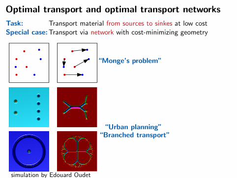
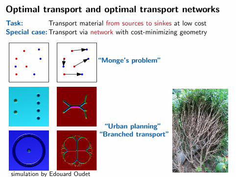
Task: Transport material from sources to sinkes at low costSpecial case: Transport via network with cost-minimizing geometry
“Monge’s problem”
simulation by Edouard Oudet
“Urban planning”“Branched transport”

Optimal transport and optimal transport networks
Task: Transport material from sources to sinkes at low costSpecial case: Transport via network with cost-minimizing geometry
“Monge’s problem”
simulation by Edouard Oudet
“Urban planning”“Branched transport”
Optimal transport and optimal transport networks
Task: Transport material from sources to sinkes at low costSpecial case: Transport via network with cost-minimizing geometry
“Monge’s problem”
simulation by Edouard Oudet
“Urban planning”“Branched transport”
Optimal transport and optimal transport networks
Task: Transport material from sources to sinkes at low costSpecial case: Transport via network with cost-minimizing geometry
“Monge’s problem”
simulation by Edouard Oudet
“Urban planning”“Branched transport”

Models for transport networks: Intuition
cost functional = transport costs + network costs
network costs
∼
network length
transport costsper distance
mass
economy of scales ︸︷︷︸ ⇒ branching structures
sought: 1D pipe network Σ ⊂ Rn for transport fromµ0 toµ1
µ0
µ1
massF
cost
per
flu
x&
len
gth
urban branchedplanning transport
1 F−ε
a > 1 ∞ε 0

Are models of qualitatively different type?
µ0
µ1
massF
cost
per
flu
x&
len
gth
urban branchedplanning transport
1 F−ε
a > 1 ∞ε 0
Classical formulation urban planning
dΣ(x , y) = infaH1(γ \ Σ) +H1(γ ∩ Σ) : γ path from x to y
Eε,a[Σ] = WdΣ(µ0, µ1) + εH1(Σ)
= infµ∈fbm(Rn×Rn)
π1#µ=µ0 , π2#µ=µ1
∫Rn×Rn
dΣ(x , y)dµ(x , y) + εH1(Σ)
requires computation of dΣ or dual formulation
variation with respect to Σ nontrivial

Are models of qualitatively different type?
µ0
µ1
massF
cost
per
flu
x&
len
gth
urban branchedplanning transport
1 F−ε
a > 1 ∞ε 0
Classical formulation branched transport
G = (V ,E ) = directed weighted graph
we = flow through e ∈ E , le = length of ewe
Mε[G ] =
∑e∈E w1−ε
e le if Kirchhoff laws satisfied
∞ elsew
w1−ε
Mε[F ] = inflim infn→∞
Mε[Gn] |Gn∗ F , divF = µ0 − µ1
allows phase field description!

Are models of qualitatively different type?
µ0
µ1
massF
cost
per
flu
x&
len
gth
urban branchedplanning transport
1 F−ε
a > 1 ∞ε 0
New formulation urban planning [Brancolini, Wirth ’15]
G = (V ,E ) = directed weighted graph
we = flow through e ∈ E , le = length of ewe
Ea,ε[G ] =
∑e∈E ca,ε(w)le if Kirchhoff laws satisfied
∞ sonstw
ca,ε(w)
Ea,ε[F ] = inflim infn→∞
Mε[Gn] |Gn∗ F , divF = µ0 − µ1
Thm. minΣ Ea,ε[Σ] = minF Ea,ε[F ] & Σopt ⊂ sptFopt

Analysis of optimal geometries
µ0
µ1
massF
cost
per
flu
x&
len
gth
urban branchedplanning transport
1 F−ε
a > 1 ∞ε 0
Near-optimal networks
µ0
µ1
-
6?
length scales in terms of powers of ε
Thm. cf (ε, a) ≤ minΣJ ε,a[Σ]− J ∗ ≤ Cf (ε, a)
f (ε, a) =
ε
23 urban planning 2D (J ε,a = Eε,a)√ε(√a + | log a−1√
ε|) urban planning 3D (J ε,a = Eε,a)
ε1
n−1√a√a− 1
n−3n−1 urban planning nD (J ε,a = Eε,a)
ε| log ε| branched transport (J ε,a =Mε)

Analysis of optimal geometries
µ0
µ1
massF
cost
per
flu
x&
len
gth
urban branchedplanning transport
1 F−ε
a > 1 ∞ε 0
Thm. cf (ε, a) ≤ minΣJ ε,a[Σ]− J ∗ ≤ Cf (ε, a)
f (ε, a) =
ε
23 urban planning 2D (J ε,a = Eε,a)√ε(√a + | log a−1√
ε|) urban planning 3D (J ε,a = Eε,a)
ε1
n−1√a√a− 1
n−3n−1 urban planning nD (J ε,a = Eε,a)
ε| log ε| branched transport (J ε,a =Mε)
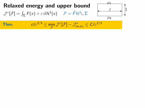
Relaxed energy and upper bound
µ0
µ1
6
?
1- `J ε[F ] =
∫Σ F (x) + εdH1(x) F = ~FH1xΣ
Thm. c`ε2/3 ≤ minFJ ε[F ]− J ∗µ0,µ1
≤ C`ε2/3
Step 1: Relaxation for ε = 0given source µa & sink µb,J ∗µa,µb := infJ 0[F ] | F transports µa to µb
= Wasserstein-distance(µa, µb)
J ∗µa,µb can be computed/accurately estimated!(e. g. via convex duality) ⇒ J ∗µ0,µ1
= `
Step 2: Upper bound by construction
µ0
µ1level
1
1
2
2
3
3elementary cell
-w?6h
w1 ∼ 3√ε
hi =√w3i /ε

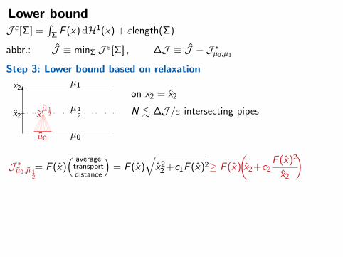
Lower boundJ ε[Σ] =
∫Σ F (x)dH1(x) + εlength(Σ)
abbr.: J ≡ minΣ J ε[Σ] , ∆J ≡ J − J ∗µ0,µ1
Step 3: Lower bound based on relaxation
µ0
µ1
. .. . . . . . . . . . . . .µ 12
6
x2
x2on x2 = x2
N . ∆J /ε intersecting pipes
µ0
µ 12x
J ∗µ0,µ 12
= F (x)( average
transportdistance
)= F (x)
√x2
2 +c1F (x)2≥ F (x)
(x2+c2
F (x)2
x2
)
J ≥ J ∗µ0,µ 12
+J ∗µ 12,µ1≥∑
x∈suppµ0
[x2F (x)+c F (x)3
x2
]+[(1− x2)F (x)+c F (x)3
1−x2
]≥ `+
∑x∈suppµ0
c F (x)3
12
≥ J ∗µ0,µ1+ 2c`( `N )2 ≥ J ∗µ0,µ1
+ 2c`( ε`∆J )2

Analysis & numerics in 2D via imagesµ1
µ0
F
u
-`
6
?
1
-6
6
x1
x2
F ∈ fbm(Ω;R2)
divF = µ0 − µ1
u ∈ BV(Ω;R)
u(x1, 0) =∫x2=0,x1≤x1 dµ0(x)
u(x1, 1) =∫x2=0,x1≤x1 dµ1(x)
One-to-one relation fluxes ↔ images: Fu = ∇u⊥, Σ = Su∫Ω
φ d(divFu) = −∫
Ω
∇φ·dFu =
∫Ω
∇φ⊥ ·d∇u = −∫
Ω
div(∇φ⊥)u dx = 0 ∀φ ∈ C∞c (Ω)
... with boundary terms: divFu = µ0 − µ1

Network functionals in terms of images
µ0
µ1 flux F
cost
per
flu
x&
len
gth
urban branchedplanning transport
1 F−ε
a > 1 ∞ε 0
Versions of Mumford–Shah segmentation ...
M.-S.: J ε,a[u] =
∫Ω\Su
a(u − u)2 + |∇u|2dx +
∫Su
ε dH1
urb. pl.: Eε,a[u] =
∫Ω\Su a|∇u| dx +
∫Su|[u]|+εdH1 if u satisfies b. c.
∞ else
br. tpt.: Mε[u] =
∫Su|[u]|1−ε dH1 if u satisfies b. c. and ∇u ≡ 0
∞ else

Network functionals in terms of images
µ0
µ1 flux F
cost
per
flu
x&
len
gth
urban branchedplanning transport
1 F−ε
a > 1 ∞ε 0
Versions of Mumford–Shah segmentation ...
M.-S.: J ε,a[u] =
∫Ω\Su
g(x , u,∇u) dx +
∫Su
ψ(x , u+, u−, ν)dH1
urb. pl.: Eε,a[u] =
∫Ω\Su a|∇u| dx +
∫Su|[u]|+εdH1 if u satisfies b. c.
∞ else
br. tpt.: Mε[u] =
∫Su|[u]|1−ε dH1 if u satisfies b. c. and ∇u ≡ 0
∞ else

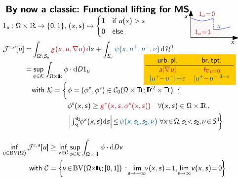
By now a classic: Functional lifting for MS
1u : Ω×R→ 0, 1, (x , s) 7→
1 if u(x) > s
0 else
x
s
u1u =1
1u =0
J ε,a[u] =
∫Ω\Su
g(x , u,∇u)dx +
∫Su
ψ(x , u+, u−, ν)dH1
= supφ∈K
∫Ω×R
φ · dD1u
with K =
φ = (φx , φs) ∈ C0(Ω×R;R2 ×R) :
φs(x , s) ≥ g∗(x , s, φx(x , s)) ∀(x , s) ∈ Ω×R ,∣∣∣∫ s2
s1φx(x, s)ds
∣∣∣≤ψ(x, s1, s2, ν) ∀x ∈Ω, s1<s2, ν∈S1
urb. pl. br. tpt.
a|∇u| I∇u=0
|u+−u−|+ε |u+−u−|1−ε
infu∈BV(Ω)
J ε,a[u] ≥ infv∈C
supφ∈K
∫Ω×R
φ · dDv
with C =
v ∈BV(Ω×R; [0, 1]) : lim
s→−∞v(x , s)=1, lim
s→∞v(x , s)=0
Lower bound on network costs
Urban planning: g(x , u,∇u) = a|∇u|, ψ(x , s1, s2, ν) = |s1 − s2|+ ε
K =φ = (φx , φs) : φs ≥ 0,|φx | ≤ a,
∣∣∣∫ s2
s1φx(x, s)ds
∣∣∣≤|s2 − s1|+ ε
Branched transport: g(x , u,∇u) = I∇u=0, ψ(x , s1, s2, ν) = |s1 − s2|1−ε
K =φ = (φx , φs) : φs ≥ 0,
∣∣∣∫ s2
s1φx(x, s)ds
∣∣∣≤|s2 − s1|1−ε
Lower bound: J ε,a = Eε,a, J ε,a =Mε
mindivF=µ0−µ1
J ε,a[F ] = minu|∂Ω(x)=x1
J ε,a[u] ≥ infv |∂(Ω×R)=1x 7→x1
supφ∈K
∫Ω×R
φ · dDv
= supφ∈K
infv |∂(Ω×R)=1x 7→x1
∫∂Ω
∫ x1
−∞φ · ν ds dx−
∫Ω×R
vdivφd(x , s)
≥ supφ∈K,divφ=0,φs=0
∫∂Ω
∫ x1
−∞φ · ν ds dx

Lower bound on network costs
Urban planning: g(x , u,∇u) = a|∇u|, ψ(x , s1, s2, ν) = |s1 − s2|+ ε
K =φ = (φx , φs) : φs ≥ 0,|φx | ≤ a,
∣∣∣∫ s2
s1φx(x, s)ds
∣∣∣≤|s2 − s1|+ ε
Branched transport: g(x , u,∇u) = I∇u=0, ψ(x , s1, s2, ν) = |s1 − s2|1−ε
K =φ = (φx , φs) : φs ≥ 0,
∣∣∣∫ s2
s1φx(x, s)ds
∣∣∣≤|s2 − s1|1−ε
Lower bound: J ε,a = Eε,a, J ε,a =Mε
mindivF=µ0−µ1
J ε,a[F ] = minu|∂Ω(x)=x1
J ε,a[u] ≥ supφ∈K
infv |∂(Ω×R)=1x 7→x1
∫Ω×R
φ · dDv
= supφ∈K
infv |∂(Ω×R)=1x 7→x1
∫∂Ω
∫ x1
−∞φ · ν ds dx−
∫Ω×R
vdivφ d(x , s)
≥ supφ∈K,divφ=0,φs=0
∫∂Ω
∫ x1
−∞φ · ν ds dx

Construction for φexpected optimal image
mindivF=µ0−µ1
J ε,a[F ] = minu|∂Ω(x)=x1
J ε,a[u]
corresponding lifting
mindivF=µ0−µ1
J ε,a[F ] ≥ supdivxφx=0, |φx |≤a∣∣∣∫ s2
s1φx (x,s)ds
∣∣∣≤h(|s2−s1|)
∫∂Ω
∫ x1
−∞φx·νxdxds
h(s) =
s+ε urb. pl.s1−ε br. tpt.
test field φ

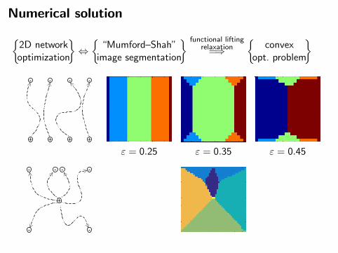
Numerical solution
2D networkoptimization
⇔
“Mumford–Shah”image segmentation
functional liftingrelaxation=⇒
convex
opt. problem
ε = 0.25 ε = 0.35 ε = 0.45
Numerical solution
2D networkoptimization
⇔
“Mumford–Shah”image segmentation
functional liftingrelaxation=⇒
convex
opt. problem
ε = 0.25 ε = 0.35 ε = 0.45

Networks in real life

Networks in real life

Networks in real life


![OPTIMAL TRANSPORT IN GEOMETRY · Optimal transport is one such tool References • Topics in Optimal Transportation [TOT] (AMS, 2003): Introduction • Optimal transport, old and](https://static.documents.pub/doc/80x56/5ec621bb8d12144b8d424d3b/optimal-transport-in-geometry-optimal-transport-is-one-such-tool-references-a.jpg)


