+ All Categories
Home > Documents > OPTIMUM DESIGN OF RIGID AND SEMI-RIGID STEEL …etd.lib.metu.edu.tr/upload/12612281/index.pdf ·...

OPTIMUM DESIGN OF RIGID AND SEMI-RIGID STEEL …etd.lib.metu.edu.tr/upload/12612281/index.pdf ·...

Date post: 27-Jun-2018
Category:
Upload: vokien
View: 221 times
Download: 0 times
Share this document with a friend
262
ii OPTIMUM DESIGN OF RIGID AND SEMI-RIGID STEEL SWAY FRAMES INCLUDING SOIL- STRUCTURE INTERACTION A THESIS SUBMITTED TO THE GRADUATE SCHOOL OF NATURAL AND APPLIED SCIENCES OF MIDDLE EAST TECHNICAL UNIVERSITY BY ERKAN DOĞAN IN PARTIAL FULFILLMENT OF THE REQUIREMENTS FOR THE DEGREE OF DOCTOR OF PHILOSOPHY IN ENGINEERING SCIENCES AUGUST 2010
Transcript

ii

OPTIMUM DESIGN OF RIGID AND SEMI-RIGID STEEL SWAY FRAMES INCLUDING SOIL- STRUCTURE INTERACTION

A THESIS SUBMITTED TO THE GRADUATE SCHOOL OF NATURAL AND APPLIED SCIENCES

OF MIDDLE EAST TECHNICAL UNIVERSITY

BY

ERKAN DOĞAN

IN PARTIAL FULFILLMENT OF THE REQUIREMENTS FOR

THE DEGREE OF DOCTOR OF PHILOSOPHY IN

ENGINEERING SCIENCES

AUGUST 2010

ii

Approval of the thesis

OPTIMUM DESIGN OF RIGID AND SEMI-RIGID STEEL SWAY FRAMES INCLUDING SOIL - STRUCTURE INTERACTION

submitted by ERKAN DOĞAN in partial fulfillment of the requirements for the degree of Doctor of Philosophy in Engineering Sciences Department, Middle East Technical University by,

Prof. Dr. Canan ÖZGEN ________________ Dean, Graduate School of Natural and Applied Sciences Prof. Dr. Turgut TOKDEMİR ________________ Head of Department, Engineering Sciences Prof. Dr. Mehmet Polat SAKA ________________ Supervisor, Engineering Sciences Dept., METU Prof. Dr. Turgut TOKDEMİR ________________ Co- Supervisor, Engineering Sciences Dept., METU

Examining Committee Members :

Prof. Dr. Ayşe DALOĞLU ________________ Civil Engineering Dept., KTU Prof. Dr. Mehmet Polat SAKA ________________ Engineering Sciences Dept., METU Prof. Dr. Ayşe Gülin BİRLİK ________________ Engineering Sciences Dept., METU Assoc. Prof. Dr. Oğuzhan HASANÇEBİ ________________ Civil Engineering Dept., METU Assoc. Prof. Dr. Zafer EVİS ________________ Engineering Sciences Dept., METU

Date :

iii

I hereby declare that all information in this document has been obtained and presented in accordance with academic rules and ethical conduct. I also declare that, as required by these rules and conduct, I have fully cited and referenced all material and results that are not original to this work. Name, Surname : Erkan DOĞAN

Signature :

iv

ABSTRACT

OPTIMUM DESIGN OF RIGID AND SEMI-RIGID STEEL SWAY FRAMES INCLUDING SOIL- STRUCTURE INTERACTION

Doğan, Erkan

Ph.D., Engineering Sciences Department

Supervisor: Prof. Dr. M. Polat Saka

Co-Supervisor: Prof. Dr. Turgut Tokdemir

August 2010, 240 Pages

In this study, weight optimization of two dimensional steel frames is carried out in

which the flexibility of beam-to-column connections and the soil-structure

interaction are considered. In the analysis and design of steel frames, beam-to-

column connections are assumed to be either fully rigid or perfectly pinned.

However, the real behavior of beam-to-column connections is actually between

these extremes. Namely, even the simple connections used in practice possess some

stiffness falling between these two cases mentioned above. Moreover, it is found

that there exists a nonlinear relationship between the moment and beam-to-column

rotation when a moment is applied to a flexible connection. These partially

restrained connections influence the drift (P-∆ effect) of whole structure as well as

the moment distribution in beams and columns. Use of a direct nonlinear inelastic

analysis is one way to account for all these effects in frame design. To be able to

implement such analysis, beam-to-column connections should be assumed and

v

modeled as semi-rigid connections. In the present study, beam-to-column

connections are modeled as “end plate without column stiffeners” and “top and seat

angle with web angles”. Soil-structure interaction is also included in the analysis.

Frames are assumed to be resting on nonlinear soil, which is represented by a set of

axial elements. Particle swarm optimization method is used to develop the optimum

design algorithm. The Particle Swarm method is a numerical optimization technique

that simulates the social behavior of birds, fishes and bugs. In nature fish school,

birds flock and bugs swarm not only for reproduction but for other reasons such as

finding food and escaping predators. Similar to birds seek to find food, the optimum

design process seeks to find the optimum solution. In the particle swarm

optimization each particle in the swarm represents a candidate solution of the

optimum design problem. The design algorithm presented selects sections for the

members of steel frame from the complete list of sections given in LRFD- AISC

(Load and Resistance Factor Design, American Institute of Steel Construction).

Besides, the design constraints are implemented from the specifications of the same

code which covers serviceability and strength limitations. The optimum design

algorithm developed is used to design number of rigid and semi-rigid steel frames.

Keywords: Optimum structural design, soil-structure interaction, particle swarm

algorithm, minimum weight, semi-rigid connections, combinatorial optimization,

steel frames.

vi

ÖZ

RİJİT VE YARI-RİJİT ÇELİK ÇERÇEVELERİN ZEMİN-YAPI ETKİLEŞİMİNİ DE İÇEREN OPTİMUM BOYUTLANDIRILMASI

Doğan, Erkan

Doktora, Mühendislik Bilimleri Bölümü

Tez Danışmanı: Prof. Dr. M. Polat Saka

Ortak tez Danışmanı: Prof. Dr. Turgut Tokdemir

Ağustos 2010, 240 Sayfa

Bu çalışmada, iki boyutlu çelik çerçevelerin kiriş-kolon bağlantısının esnekliğini ve

zemin-yapı etkileşimini gözönüne alarak ağırlık optimizasyonu yapılmıştır. Çelik

çerçevelerin analiz ve tasarımında kiriş-kolon bağlantılarının ya tam rijit ya da tam

mafsallı olduğu kabul edilmektedir. Fakat, kiriş-kolon bağlantılarının gerçek

davranışı bu iki durumun arasındadır. Pratikte kullanılan basit bağlantılar bile

yukarıda belirtilen iki durumun arasında kalan bir rijitliğe sahiptirler. Öte yandan

esnek bağlantıya moment uygulandığında, kiriş-kolon dönme açısı ile uygulanan

moment arasında lineer olmayan bir bağlantının varlığı bulunmuştur. Bu tür kısmi

tutulmuş bağlantılar tüm yapının yanal deplasmanını (P-∆ etkisi) ve kiriş ve

kolonlardaki moment dağılımını etkilemektedir. Doğrudan lineer ve elastik olmayan

analiz yöntemi kullanmak, bu etkilerin çerçeve tasarımındaki etkisini hesaba

katmak için var olan yöntemlerden birisidir. Bu tür bir analiz yapmak için kiriş-

kolon bağlantısı yarı-rijit olarak kabul edilmeli ve ona göre modellenmelidir. Bu

çalışmada kiriş-kolon bağlantıları “kolon berkitmeleri olmayan uç levhalı” ve “üst,

vii

alt ve gövdelerinde korniyer” kullanılan türde bağlantılar olarak modellenmiştir.

Analizde zemin-yapı etkileşimi de göz önüne alınmıştır. Çerçevelerin bir grup

eksenel elemanlarla temsil edilen lineer olmayan bir zemine oturduğu

varsayılmıştır. Optimum boyutlandırma algoritmasının geliştirilmesinde parçacık

kümesi optimizasyonu metodu kullanılmıştır. Parçacık kümesi yöntemi kuşların,

balıkların ve böceklerin sosyal davranışını simule eden bir sayısal optimizasyon

tekniğidir. Doğada balıklar, kuşlar ve böcekler sadece üreme için değil, yemek

bulma ve düşmanlarından kaçma gibi diğer sebeplerden dolayı da sürü halinde

olurlar. Kuşların yemek aramasına benzer olarak, optimum boyutlandırma işlemi

de, optimum çözümü arar. Parçacık küme optimizasyonunda kümedeki her parçacık

optimum boyutlandırma probleminin aday çözümünü temsil eder. Sunulan

boyutlandırma algoritması, LRFD-AISC (Yük ve Direnç Faktörü Tasarımı-

Amerikan Çelik Konstrüksiyon Enstitüsü) de verilen w-profillerinin tümünün

bulunduğu listeden çelik çerçevenin elemanları için w-profili seçer. Ayrıca dayanım

ve deplasman sınırlarını kapsayan aynı şartnamede belirlenmiş kısıtlar, optimum

boyutlandırma probleminin sınırlayıcıları olarak uygulanmıştır. Geliştirilen

optimum boyutlandırma algoritması ile rijit ve yarı-rijit çelik çerçevelerin tasarımı

yapılmıştır.

Anahtar Kelimeler: Optimum boyutlandırma, parçacık sürü optimizasyonu

yöntemi, minimum ağırlık, zemin-yapı etkileşimi, yarı-rijit bağlantı noktaları, çelik

çerçeveler.

viii

To my family

ix

ACKNOWLEDGEMENTS

I would like to express my deepest gratitude to my thesis supervisor Prof. Dr. M.

Polat SAKA for his guidance, understanding, kind support, encouraging advices,

criticism, and valuable discussions throughout my thesis.

I am greatly indebted to Prof. Dr. M. Ruşen GEÇİT and Prof. Dr. Turgut TOKDEMİR

for their guidance and providing me every opportunity to use in Engineering

Sciences Department.

I would sincerely thank to Hakan BAYRAK, Ferhat ERDAL, Fuat KORKUT, and

Semih ERHAN for their endless friendship, making my stay in METU happy and

memorable and being always right beside me.

I would also like to thank to my friends Özge ERDEMLİ, Serdar ÇARBAŞ, Refik

Burak TAYMUŞ, İbrahim AYDOĞDU, Memduh KARALAR, Alper AKIN, Mehmet

DOĞAN, Kaveh HASSANZEHTAB, Ali GÖK, Engin KURŞUN, Fatih GÖKÇE, Ali

Sinan DİKE and E. Emre ÇALIK, for cooperation and friendship, and helping me in

all the possible ways.

My greatest thanks go to my parents, Perihan DOĞAN and Adnan DOĞAN for their

support, guidance and inspiration all through my life, my sisters Nurhan DOĞAN

and Tuğçe DOĞAN who are always there for me.

I dedicate this dissertation to my aunt İhame DOĞAN, my uncle Özkan KIRKPINAR,

his wife Arzu KIRKPINAR and every other members of my family who always

offered their advice, love, care and support. My family’s absolute unquestionable

belief in me, have been a constant source of encouragement and have helped me

achieve my goals.

x

TABLE OF CONTENTS

ABSTRACT ............................................................................................................. iv ÖZ………. ................................................................................................................ vi ACKNOWLEDGEMENTS .................................................................................... ix TABLE OF CONTENTS ........................................................................................ x LIST OF TABLES ................................................................................................ xvi LIST OF FIGURES ............................................................................................ xviii LIST OF ABBREVIATIONS………………………………………………......xxii CHAPTERS 1 INTRODUCTION ............................................................................................. 1

1.1 Modeling of steel frames............................................................................. 1

1.2 Semi-Rigid Steel Frames ............................................................................ 2

1.3 Soil-Structure Interaction ............................................................................ 3

1.4 Optimization ............................................................................................... 4

1.4.1 Optimization models ........................................................................... 7

1.4.1.1 Continuous-variable models ........................................................ 7

1.4.1.2 Discrete-variable models ............................................................. 8

1.4.2 Structural optimization ........................................................................ 8

1.4.2.1 Structural Optimization Problems ............................................. 11

1.4.2.1.1 Sizing Optimization Problems ........................................... 13

1.4.2.1.2 Shape Optimization Problems ........................................... 14

1.4.2.1.3 Topology Optimization Problems ...................................... 15

1.4.2.2 Structural Optimization Methods .............................................. 16

1.4.2.2.1 Analytical Methods ............................................................ 16

xi

1.4.2.2.2 Numerical Methods ............................................................ 17

1.4.2.2.2.1 Mathematical Programming ....................................... 20

1.4.2.2.2.2 Optimality Criteria ..................................................... 22

1.4.3 Stochastic search methods ................................................................. 23

1.4.3.1 Genetic algoritms ....................................................................... 24

1.4.3.2 Tabu Search ............................................................................... 25

1.4.3.3 Evalution Strategies ................................................................... 26

1.4.3.4 Simulated Annealing ................................................................. 27

1.4.3.5 Ant Colony Optimization .......................................................... 28

1.4.3.6 Harmony Search Algorithm....................................................... 31

1.4.3.7 Big bang- big crunch Optimization ........................................... 32

1.4.3.8 Particle Swarm Optimization ..................................................... 33

1.4.4 Constraint Handling Methods ........................................................... 34

1.4.4.1 Penalty Functions Method ......................................................... 35

1.4.4.2 Fly-back Mechanism ................................................................. 38

1.5 Literature Survey....................................................................................... 38

1.6 Scope of Work .......................................................................................... 40

2 PARTICLE SWARM ALGORITHM .......................................................... 42

2.1 Introduction ............................................................................................... 42

2.1.1 Swarm Intelligence. ........................................................................... 42

2.1.2 Evolutionary Computation. ............................................................... 44

2.2 Particle Swarm Algorithm ........................................................................ 45

2.2.1 Inertia Weight. ................................................................................... 49

2.2.2 Control Parameters ............................................................................ 49

2.2.3 Vmax. ................................................................................................ 49

2.2.4 Neighborhood Topology ................................................................... 50

2.3 Particle Swarm Optimization in Continuous Design Space ...................... 52

2.3.1 Numerical Examples in Continuous Design Space. .......................... 52

2.3.1.1 Example 1 .................................................................................. 52

xii

2.3.1.2 Example 2 ............................................................................... 56

2.3.1.3 Example 3 ............................................................................... 61

2.3.1.4 Example 4 .................................................................................. 63

2.4 Particle Swarm Optimization in Discrete Design Space ........................... 67

2.4.1 Numerical Examples in Discrete Design Space. ............................... 70

2.4.1.1 Example 1 .................................................................................. 70

2.4.1.2 Example 2 ............................................................................... 72

3 OPTIMUM DESIGN OF RIGIDLY CONNECTED STEEL SWAY

FRAMES TO LRFD ....................................................................................... 74

3.1 Steel Frames .............................................................................................. 74

3.2 Analysis of Frames.................................................................................... 76

3.2.1 Matrix Stiffness Method .................................................................... 76

3.2.1.1 Analytical Model ....................................................................... 77

3.2.1.1.1 Global and Local Coordinate System ................................ 78

3.2.1.1.2 Relationship between Local and global Coordinates ......... 80

3.2.1.1.3 Degrees of Freedom .......................................................... .81

3.2.1.1.4 Relationship between Member End Forces and Member End Deformations… .............................. ………………....83

3.2.1.1.5 Relationship between the Joint Displacements and Member End Deformations…… .............................. ….….89

3.2.1.1.6 Relationship between External Loads and Member Forces………… ........................................................ …….91

3.3 Load and Resistance Factor Design for Rolled Beam-columns………………… ........................................... ………..…93

3.3.1 Compact sections…………… ......................................... ….…...….96

3.3.2 Non-compact sections…………… ............................... ……….......97

3.3.3 Partially Compact Sections … ............................... ……………......98

3.3.4 Slender Sections …… .............................. .…………………….......98

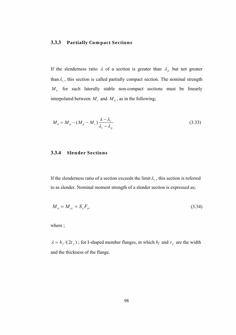
3.3.5 Load and Resistance Factor Design for Combined Strength in Rolled Beam- columns … ................................. ………………….100

xiii

3.3.5.1 Load and Resistance Factor Design for Beam-columns subject to Bending and Axial tension ...................................... 100

3.3.5.2 Load and Resistance Factor Design for Beam-columns subject to Bending and Axial compression ............................. 102

3.3.5.2.1 Effective Length of a Beam-column Member ................. 103

3.3.6 Load and Resistance Factor Design for Shear in Rolled Beam-columns. ............................................................................... 105

3.3.7 Load and Resistance Factor Design for Serviceability of Beam-columns. ............................................................................... 107

3.3.7.1 Deflection ................................................................................ 108

3.3.7.2 Drift ......................................................................................... 109

3.3.7.3 Geometric Compatibility ......................................................... 110

3.4 Optimum Design of Steel Frames ........................................................... 111

3.4.1 Mathematical Model of Optimum Design Problem of Unbraced Steel Frames. .................................................................. 112

3.4.2 Optimum Design of Steel Frames in Continuous Design Space .... 115

3.4.3 Optimum Design of Steel Frames in Discrete Design Space ......... 118

3.4.4 Particle Swarm Optimization Design of Unbraced Steel Frames .. 119

3.4.5 Design Examples ............................................................................ 120

3.4.5.1 Three Storey, Two Bay Steel Frame ....................................... 121

3.4.5.2 Four Storey, Four Bay Steel Frame ......................................... 123

3.4.5.3 Five Storey, Three Bay Steel Frame ........................................ 125

3.4.5.4 Six Storey, Two Bay Steel Frame ........................................... 128

3.4.5.5 Ten Storey, One Bay Steel Frame ........................................... 131

3.4.5.6 Ten Storey, Three Bay Steel Frame......................................... 134

3.4.5.7 Fifteen Storey, Three Bay Steel Frame ................................... 137

4 OPTIMUM DESIGN OF SEMI-RIGID STEEL SWAY FRAMES TO

LRFD .............................................................................................................. 141

4.1 Semi-Rigid Connections ......................................................................... 141

4.2 Types of Semi-Rigid Connections .......................................................... 148

xiv

4.2.1 Single Web-angle Connections and Single Plate Connections ....... 148

4.2.2 Double Web-angle Connections ...................................................... 149

4.2.3 Top and Seat Angle Connections .................................................... 150

4.2.4 Top and Seat Angle Connections with Double Web Angle ............ 151

4.2.5 Extended End – Plate Connections and Flush End-Plate Connections. ................................................................................... 151

4.2.6 Header Plate Connections ............................................................... 154

4.3 Modeling of Semi-Rigid Connections .................................................... 155

4.3.1 Polynomial Model ........................................................................... 156

4.4 Analysis of Unbraced Steel Frames with Semi-Rigid Connections ....... 158

4.4.1 End-plate without Column Stiffeners Model .................................. 163

4.4.2 Top and Seat Angle with Web Cleats Model .................................. 166

4.5 Particle Swarm Optimization Design of Unbraced Steel Frames with Semi-Rigid Connections .......................................................................... 174

4.6 Design Examples..................................................................................... 175

4.6.1 Three Storey, Two Bay Steel Frame ............................................... 176

4.6.2 Four storey, four bay steel frame .................................................... 179

4.6.3 Five storey, three bay steel frame .................................................... 181

4.6.4 Six Storey, Two Bay Steel Frame ................................................... 184

4.6.5 Ten Storey, Three Bay Steel Frame ................................................ 188

4.6.6 Fifteen Storey, Three Bay Steel Frame ........................................... 191

5 OPTIMUM DESIGN OF RIGID AND SEMI-RIGID STEEL SWAY

FRAMES INCLUDING SOIL-STRUCTURE INTERACTION ............. 195

5.1 Characteristics of Soils............................................................................ 195

5.2 Nonlinear Behavior of Soils .................................................................... 195

5.3 Soil-structure interaction ......................................................................... 198

5.3.1 Modeling the Soil-Structure Interaction .......................................... 200

5.3.1.1 Idealized Soil Behavior Models .............................................. 201

5.3.1.1.1 Elastic Models .................................................................. 201

5.3.1.1.1.1 Winklerian Spring Model ......................................... 202

xv

5.3.1.1.1.2 Elastic Continuum Models ....................................... 205

5.3.1.1.1.3 Two Parameter Elastic Models ................................ 206

5.3.1.1.1.4 Finite Element Models ............................................. 207

5.3.1.1.2 Elastic-Plastic, Perfectly Plastic Models ......................... 208

5.3.1.2 Winklerian Modeling of Planar Steel Frame-Soil Interaction System ................................................................... 209

5.4 Particle Swarm Optimization Design of Rigid and Semi-Rigid Steel Frames Including Soil-Structure Interaction ................................... 217

5.4.1 Design Examples ............................................................................. 219

5.4.1.1 Three Storey-Two Bay Steel Frame ........................................ 219

5.4.1.2 Four storey-Four Bay Steel Frame .......................................... 223

6 SUMMARY AND CONCLUSIONS ........................................................... 226

6.1 Overview and Summary of the Thesis .................................................... 226

6.2 Conclusions ............................................................................................. 228

REFERENCES .............................................................................................. 230

CV ................................................................................................................... 239

xvi

LIST OF TABLES

TABLES

Table 2.1 Sensitivity analysis of PSO parameters ................................................ 54

Table 2.2 PSO algorithm parameters used for Himmelblau’s Function .............. 55

Table 2.3 Optimum solutions for Himmelblau’s function ................................... 55

Table 2.4 PSO algorithm parameters used for welded beam design .................... 57

Table 2.5 Optimum solutions for welded beam design ........................................ 60

Table 2.6 Optimum solutions for pressure vessel design ..................................... 63

Table 2.7 Optimum solutions for spring design ................................................... 66

Table 2.8 PSO algorithm parameters used for discrete design example 1 ........... 71

Table 3.1 Optimum designs for three-storey, two-bay rigid steel frame............ 122

Table 3.2 Optimum designs for four-storey, four-bay rigid steel frame ............ 125

Table 3.3 Optimum designs for five-storey, three-bay rigid steel frame ........... 127

Table 3.4 Optimum designs for six-storey, two-bay rigid steel frame ............... 130

Table 3.5 Optimum designs for ten-storey, one-bay rigid steel frame ............... 133

Table 3.6 Optimum designs for ten-storey, three-bay rigid steel frame ............. 136

Table 3.7 Optimum designs for fifteen-storey, three-bay rigid steel frame ....... 140

Table 4.1 Standardized Connection Constants ................................................... 157

Table 4.2 Optimum designs for three-storey, two-bay rigid steel frame............ 178

Table 4.3 Optimum designs for four-storey, four-bay steel frame ..................... 180

Table 4.4 Optimum designs for five-storey, three-bay steel frame .................... 183

Table 4.5 Optimum designs for six-storey, two-bay steel frame ....................... 186

Table 4.6 Optimum designs for ten-storey, three-bay steel frame ..................... 190

Table 4.7 Optimum designs for fifteen-storey, three-bay steel frame ................ 194

Table 5.1 Stress-strain and corresponding modulus of elasticity

values of each linear segment obtained from nonlinear

xvii

stress-stress curve ............................................................................... 213

Table 5.2 Optimum designs for three-storey, two-bay steel frame .................... 222

Table 5.3 Optimum designs for four-storey, four-bay steel frame ..................... 224

xviii

LIST OF FIGURES

FIGURES

Figure 1.1 Geometry of a steel frame with semi-rigid connections ........................ 3

Figure 1.2 Two-variable optimum design problem ................................................. 6

Figure 1.3 A sizing structural optimization problem ............................................ 14

Figure 1.4 A shape optimization problem ............................................................. 14

Figure 1.5 Topology optimization of a simple truss ............................................. 15

Figure 1.6 Diagram for iterative steps of a numerical optimization method ........ 19

Figure 1.7 Path which is designed by ants to reach the destination ...................... 29

Figure 1.8 Global minimum in the feasible space ................................................. 35

Figure 2.1 Examples of swarm intelligence found in the nature ........................... 43

Figure 2.2 Demonstration of an update in the velocity vector of a particle .......... 47

Figure 2.3 Flowchart of the basic particle swarm algorithm ................................. 48

Figure 2.4 Different neighborhood topologies ...................................................... 51

Figure 2.5 Design-history graph for Himmelblau’s function ................................ 56

Figure 2.6 Welded beam design ............................................................................ 57

Figure 2.7 Design-history graph for the welded beam design .............................. 60

Figure 2.8 Pressure vessel design .......................................................................... 62

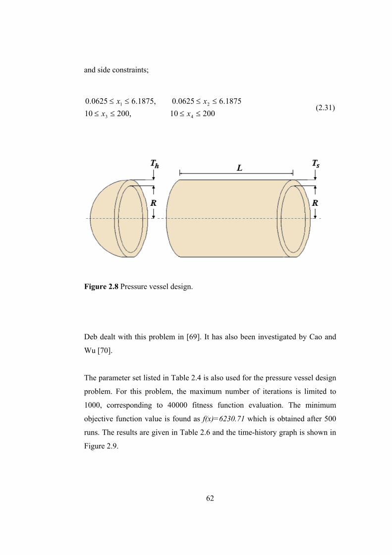
Figure 2.9 Design-history graph for the pressure vessel design ........................... 63

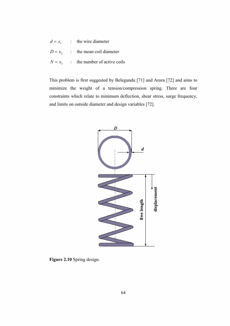
Figure 2.10 Spring design ..................................................................................... 64

Figure 2.11 Design-history graph for the spring design........................................ 67

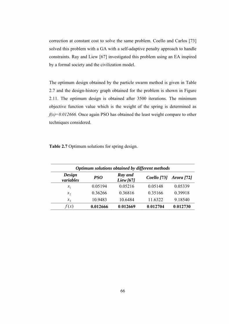
Figure 2.12 Particle swarm optimization in discrete design space ....................... 69

Figure 2.13 Contour plot of the function f (x) 2221

21 595 xxxx ........................... 71

Figure 2.14 Three Dimensional plot of the function f (x) 2221

21 595 xxxx ......... 72

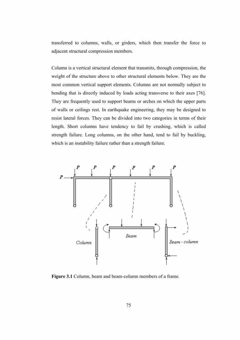
Figure 3.1 Column, beam and beam-column members of a frame ....................... 75

Figure 3.2 Analytical model of a simple frame ..................................................... 78

xix

Figure 3.3 Global and local coordinates................................................................ 79

Figure 3.4 Relationship between Global and Local axes ...................................... 81

Figure 3.5 Degrees of Freedom of a simple frame ................................................ 82

Figure 3.6 End deformations and end forces of a rigid frame member ................ 83

Figure 3.7 A small piece of a rigid frame member ............................................... 86

Figure 3.8 Derivation of the second column of the stiffness matrix [k] for rigid frame member r. ............................................................... 88

Figure 3.9 Member end forces and end displacements in local coordinates ....... 89

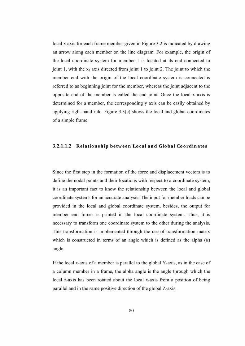
Figure 3.10 Member end forces and end displacements in global coordinates ..... 90

Figure 3.11 Most common rolled steel sections used in practice.......................... 94

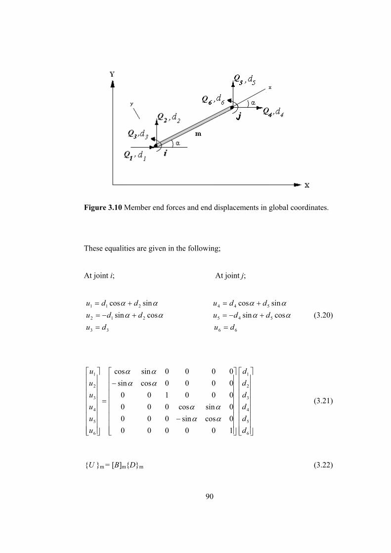
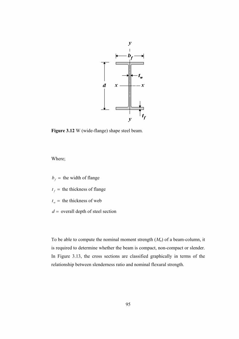
Figure 3.12 W (wide-flange) shape steel beam ..................................................... 95

Figure 3.13 Classification of cross sections for local plate buckling .................... 96

Figure 3.14 End connections of a rigid beam-column member .......................... 103

Figure 3.15 Nominal shear strength of a W section ............................................ 106

Figure 3.16 Geometry of beam to column connection ........................................ 111

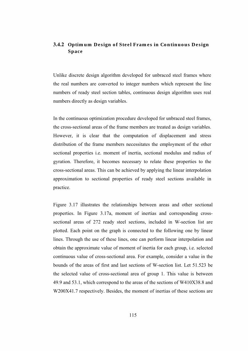
Figure 3.17 Graphical representations of cross-sectional properties of 272 W- sections. .......................................................................................... 117

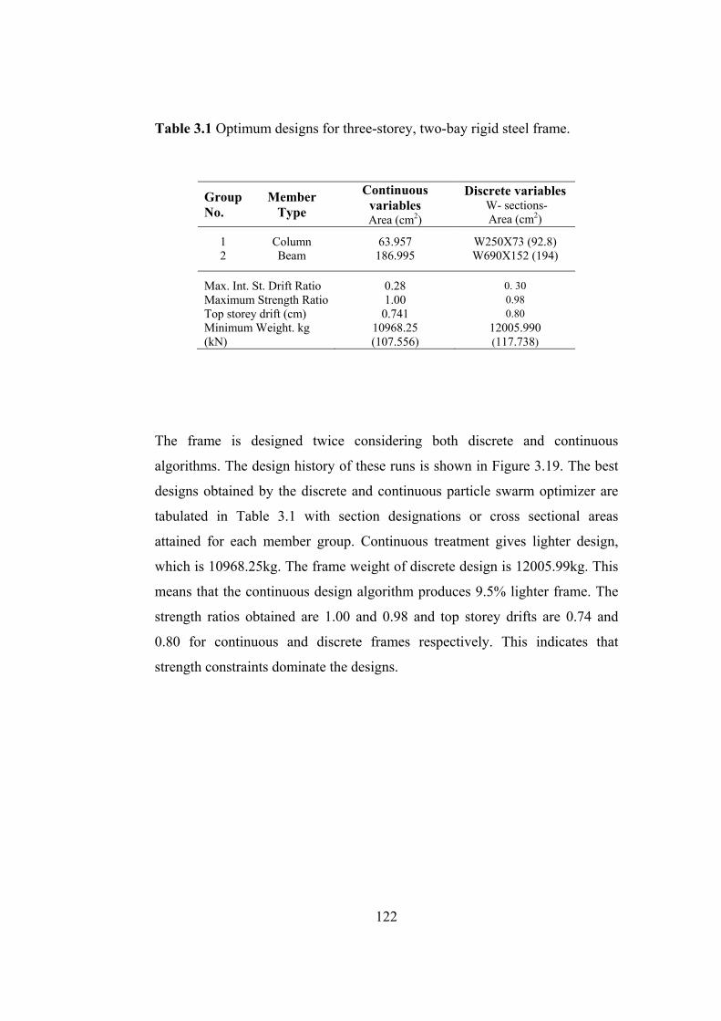
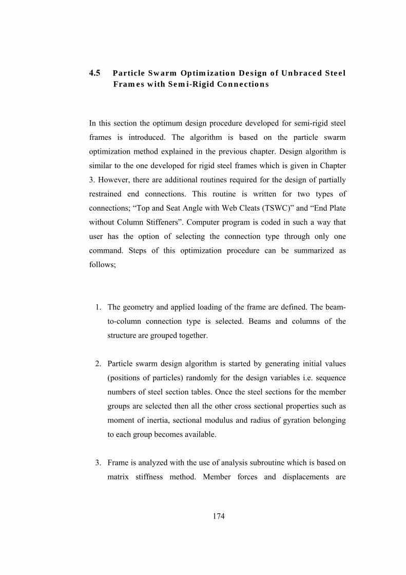
Figure 3.18 Three storey-two bay steel frame ..................................................... 121

Figure 3.19 Design history graph for three-storey, two-bay steel frame ............ 123

Figure 3.20 Four storey- four bay steel frame ..................................................... 124

Figure 3.21 Design history graph for four-storey, four-bay steel frame ............. 125

Figure 3.22 Five storey- three bay frame ............................................................ 126

Figure 3.23 Design history graph for five-storey, three-bay steel frame ............ 128

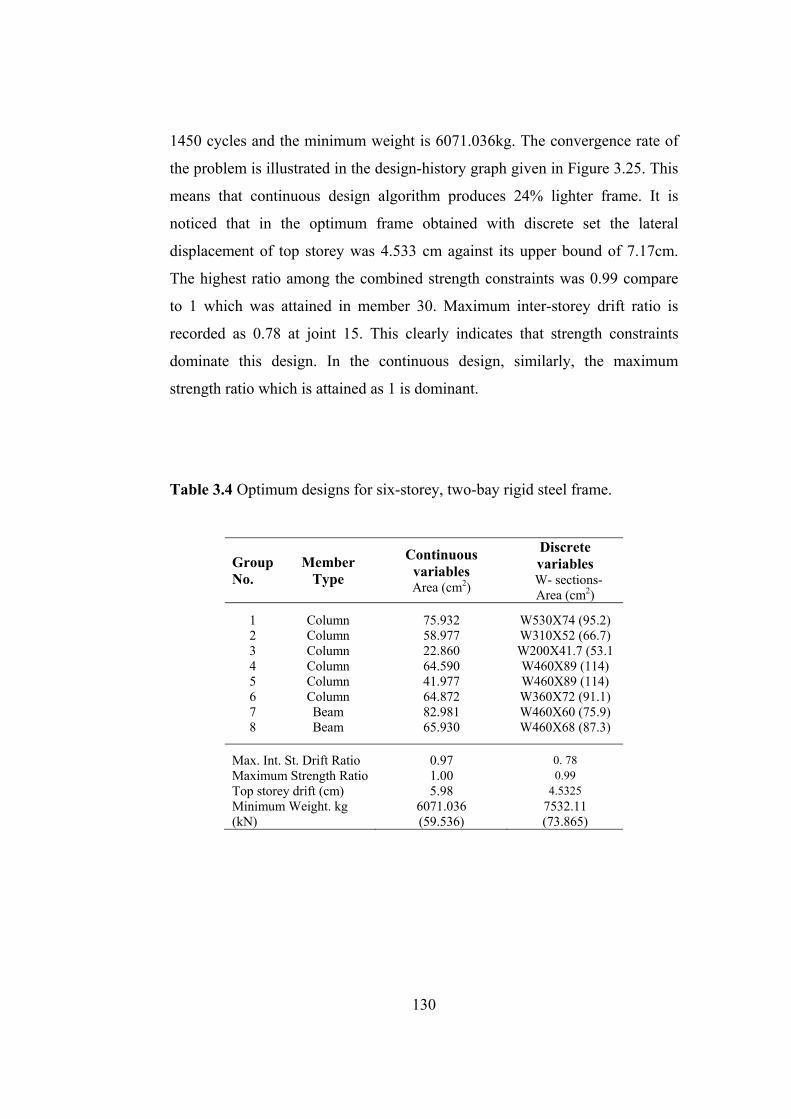
Figure 3.24 Six storey- two bay frame ................................................................ 129

Figure 3.25 Design history graph for six-storey, two-bay steel frame ................ 131

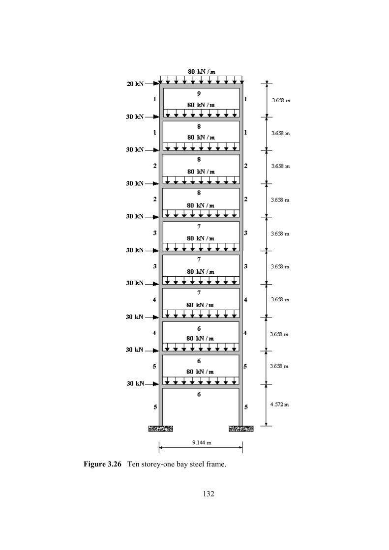
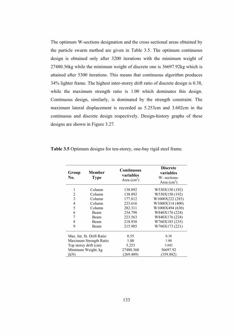
Figure 3.26 Ten storey-one bay steel frame ........................................................ 132

Figure 3.27 Design history graph for ten-storey, one-bay steel frame ................ 134

Figure 3.28 Ten storey- three bay steel frame ..................................................... 135

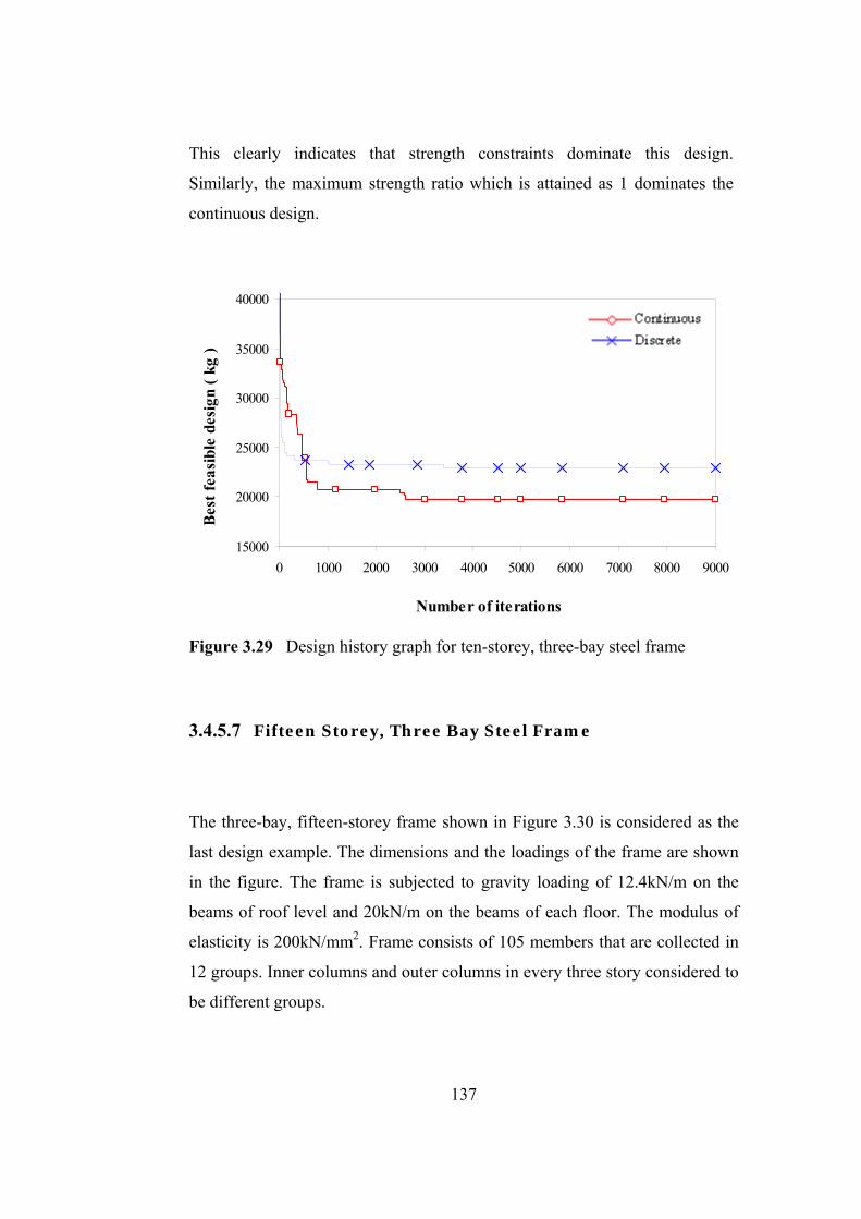
Figure 3.29 Design history graph for ten-storey, three-bay steel frame ............. 137

Figure 3.30 Fifteen-storey, three-bay steel frame ............................................... 138

xx

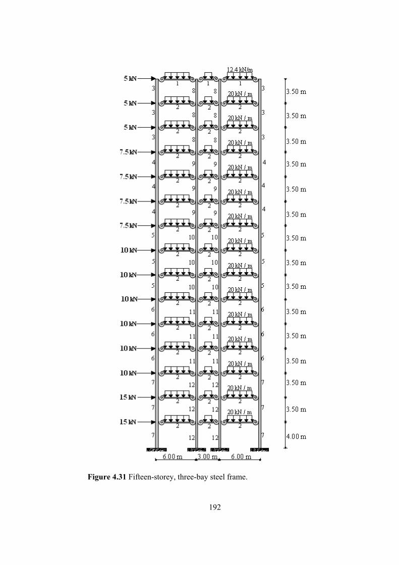
Figure 3.31 Design history graph for fifteen-storey, three-bay steel frame ........ 140

Figure 4.1 Moment- rotation behavior of connections ...................................... 142

Figure 4.2 Comparison of semi-rigid connections vs. pinned and fixed connections with respect to moment distribution. ............................... 143

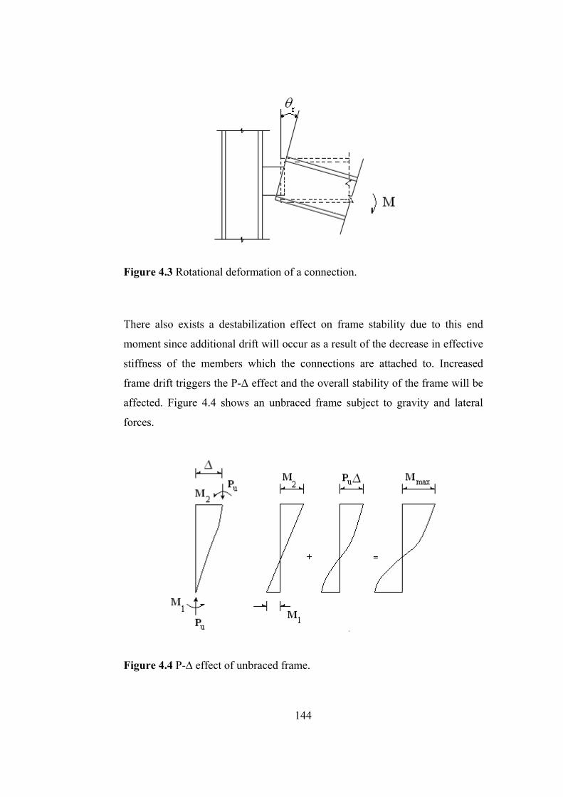
Figure 4.3 Rotational deformation of a connection .............................................. 144

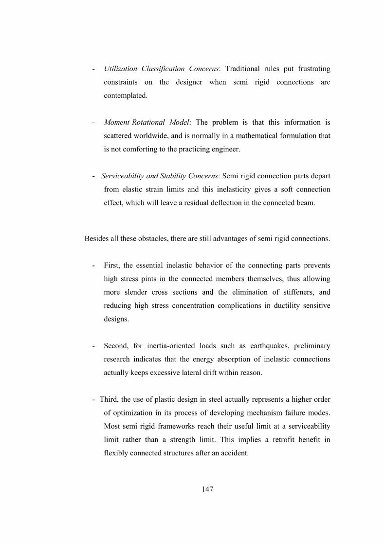
Figure 4.4 P-∆ effect of unbraced frame .............................................................. 144

Figure 4.5 Connection moment-rotation curves ................................................... 146

Figure 4.6 Single web-angle connections ............................................................ 149

Figure 4.7 Single plate connections ..................................................................... 149

Figure 4.8 Double web-angle connection ............................................................ 150

Figure 4.9 Top and seat angle connection ............................................................ 150

Figure 4.10 Top and seat angle with double web angle connection .................... 151

Figure 4.11 Extended End – Plate Connections (Tension Side Only) ................. 152

Figure 4.12 Extended End-Plate Connections (Tension and Compression Sides). ................................................... 153

Figure 4.13 Flush End-Plate Connections ............................................................ 154

Figure 4.14 Typical Header Plate Connections .................................................... 155

Figure 4.15 Semi-rigid plane beam member with rotational springs ................... 158

Figure 4.16 Moment rotation behavior of semi-rigid connection ........................ 162

Figure 4.17 End-plate without column stiffeners ................................................. 164

Figure 4.18 Top and seat angle with web cleats connection model ..................... 167

Figure 4.19 Bearing stress assumptions for seated connections .......................... 169

Figure 4.20 Top and seat angle with web cleats connection detail ...................... 170

Figure 4.21 Three storey-two bay steel frame ...................................................... 177

Figure 4.22 Design history graph for three-storey, two-bay steel frame ............. 178

Figure 4.23 Four storey- four bay steel frame ...................................................... 179

Figure 4.24 Design history graph for four-storey, four-bay steel frame .............. 181

Figure 4.25 Five storey- three bay steel frame ..................................................... 182

Figure 4.26 Design history graph for five-storey, three-bay steel frame ............. 184

Figure 4.27 Six storey- two bay steel frame......................................................... 185

xxi

Figure 4.28 Design history graph for six-storey, two-bay steel frame ................. 187

Figure 4.29 Ten storey- three bay steel frame ...................................................... 189

Figure 4.30 Design history graph for ten-storey, three-bay steel frame .............. 191

Figure 4.31 Fifteen-storey, three-bay steel frame ................................................ 192

Figure 4.32 Design history graph for fifteen-storey, three-bay steel frame ......... 194

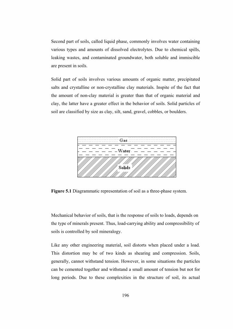
Figure 5.1 Diagrammatic representation of soil as a three-phase system ............ 196

Figure 5.2 Interaction between structure, foundation plate and soil .................... 198

Figure 5.3 Redistribution of loads in a frame due to soil–structure interaction ... 199

Figure 5.4 Surface displacements of the Winkler approach ................................. 202

Figure 5.5 Typical surface displacement profiles of an elastic continuum .......... 205

Figure 5.6 Representation of soil-structure interaction with finite element approach. ...................................................................... 208

Figure 5.7 A simple beam element with one rigid and one semi-rigid supports. ...................................................................... 210

Figure 5.8 Representation of a simple planar frame-soil interaction .................. 210

Figure 5.9 Soil-foundation-structure interaction systems ................................... 211

Figure 5.10 Stress-strain curves and Linearized load-deformation diagram ....... 212

Figure 5.11 A simple strip foundation-soil interaction problem .......................... 216

Figure 5.12 Settlements of strip foundation resting on dense silica sand ............ 217

Figure 5.13 Three storey-two bay steel frame ...................................................... 220

Figure 5.14 Design history graph for three-storey, two-bay steel frame ............. 222

Figure 5.15 Four storey-four bay steel frame ....................................................... 223

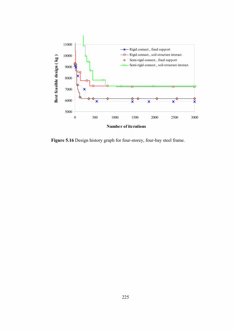
Figure 5.16 Design history graph for four-storey, four-bay steel frame .............. 225

xxii

LIST OF ABBREVIATIONS

AISC-ASD American Institute of Steel Construction-Allowable Stress

Design

CBR California Bearing Ratio

CPU Central Processing Unit

EA Evolutionary Algorithm

FR Fully Restrained

GA Genetic Algorithm

GRG Generalized Reduced Gradient

LRFD-AISC Load and Resistance Factor Design-American Institute of

Steel Construction

NPT Number of Particles

PR Partially Restrained

PSO Particle Swarm Optimization

SA Simulated Annealing

TSWC Top and Seat Angle with Web Cleats

1

CHAPTER 1

INTRODUCTION

1.1 Modeling of steel frames

Structural design is one of the prime tasks of a structural engineer. In the

design process, the first step is to select the topology of the structural systems.

In the case of steel skeletal frame, designer has to adopt steel profiles from the

steel sections table available in practice for the beams and columns of the

frame such that the response of the frame under the external loads is within the

limitations imposed by steel codes. In order to determine the behavior of the

frame, designer has to carry out structural analysis of the frame with the

selected steel sections. This necessitates structural modeling of the frame

under consideration. Designers make some assumptions particularly about

beam-to-column and column-to-support connections to simplify the analysis

problem. It is apparent that to determine the realistic behavior of a steel frame,

one has to use a realistic modeling of these connections. Determination of the

realistic behavior yields realistic design of the frame. Hence, it is important

that designer models the steel frame under consideration such that its response

to external loads is close to response of the constructed frame.

In the analysis and design of steel frames, the realistic modeling of beam-to-

column connections provides an accurate response of the frame under the

external loads. In practice, these connections are assumed to be either fully

2

rigid or perfectly pinned. In the former assumption, it is implied that there is

no relative rotation of connection and the column takes the whole end moment

of the beam. On the other hand, the pinned connection assumes that the

moment of connection is always zero and there is no existing restraint for

rotation of the connection. However, experiments have revealed that the real

behavior of beam-to-column connections is between these extremes. Namely,

all these practically used connections possess some stiffness falling between

two cases mentioned above. Moreover, it is found that there exists a nonlinear

relation of relative beam-to-column rotation when a moment is applied to a

flexible connection [1]. These partially restrained connections influence the

drift (P-∆ effect) of the whole structure as well as the moment distribution in

beams and columns. Use of a direct nonlinear inelastic analysis is one way to

account for all these effects in frame design [2]. To be able to implement such

analysis, beam-to-column connections should be assumed and modeled as

semi-rigid connections.

1.2 Semi-Rigid Steel Frames

The semi-rigid connection flexibility depends on the geometric parameters of

the elements used in beam-to-column connection such as dimensions of end

plates and bolt size. A typical steel frame with semi-rigid connections, which

is modeled by attaching rotational springs, is illustrated in Figure 1.1.

3

Figure 1.1 Geometry of a steel frame with semi-rigid connections.

1.3 Soil-Structure Interaction

Soil, as an elastic material, behaves nonlinearly after the initial loading. This

behavior is also time-dependent. This nonlinearity is the main factor of the

uncertainties of static behavior of soil-foundation-superstructure system after

construction.

Due to these uncertain behaviors of soil, the realistic structural modeling of

three dimensional buildings necessitates to consider the superstructure, its

foundation and the soil on which it rests as a complete system. This

requirement comes from the fact that any differential settlement within the

foundation system of the building effects the internal force distribution in its

members. The importance of this effect depends upon the load settlement

characteristics of the soil and the rigidity of the superstructure. In contrast to

this fact, in the analysis and design of a structure, supports are considered to

4

be either fixed or pinned without paying any attention to the characteristics of

the soil on which structure rests. The usual practice to account for the soil

under the foundation is to assume the soil as an elastic media which implies

that the reaction forces of the foundation at every point are proportional to the

deflection of the foundation at that point. This assumption leads to the

representation of the underlying soil by closely spaced, independent springs.

In some other studies, a stretched elastic membrane subjected to a constant–

tension field at the top ends of the spring was additionally introduced, in order

to achieve mathematically simple, but more realistic representation.

Furthermore, in some other works, a vertically incompressible beam was

placed on the springs which only deformed by transverse shear. There are also

finite element formulations in the literature.

1.4 Optimization

Since the earlier history, due to the limited sources in the nature, human

beings have tried to maximize the profit, economize the energy and keep the

outgoings, discomforts and pain at minimum. This phenomenon can be

possible only if the best one amongst all choices, which are the ways of

accomplishing the tasks in the course of day-to-day events, is made.

Therefore, it is required to decide upon the optimal way. The process,

optimization, as a mathematical application of this aim, is concerned with

achieving the best outcome of a given operation while satisfying certain

restrictions.

As a more general definition, the term ‘optimization’ can be defined as the

science of determining the best solution to a mathematically defined problem,

5

which is generally a model of a physical reality. Every activity in which

numerical information is processed is in the bound of applicability of

optimization.

In order to consider attaining certain goals in an optimal manner, one should

first define the objective. Objective functions defined in an optimization

problem represent some quantity, such as profit or cost that is willing to be

optimized. Afterwards, the design variables and constraints should be properly

identified on problem formulation state. Types of design variables may also

vary depending on the class of problems and needs. Constraints usually

consist of either system limitations or physical and economic laws that the

variables must satisfy. A general structural optimization problem can be

expressed as selecting optimal values of the design variables such that the

specified objective function is the minimum and constraints that are generally

non-linear functions of these variables, are satisfied. Mathematical model of a

typical optimization problem is expressed as in the following.

Minimize z = f (x) (1.1)

Subject to:

hj (x) = 0 , j = 1,2,….,0 (1.2)

gk (x) ≤ 0 , k = p+1,….,m (1.3)

xi X , X = {x1, x2,…, xq} (1.4)

where, f (x) is the objective function and x is design variable vector. In most of

the optimization problems, the constraint functions are grouped as equality

constraints hj and inequality constraints gk. In addition, some structural

6

optimization problems require the use of geometric constraints, which vary

dependent upon the type of the problem. X represents the set of design

variables and q is the total number of these variables. Number of constraints

which restrict the objective function is represented by m [3].

The selection of the objective and constraint functions defined in terms of the

quantities does condition the structural optimization design. In practice, weight

of the structure is the most commonly used objective function due to the fact

that it is readily quantified. Typical inequality constraints considered in most

structural optimization problems are displacement or/and stress limitations.

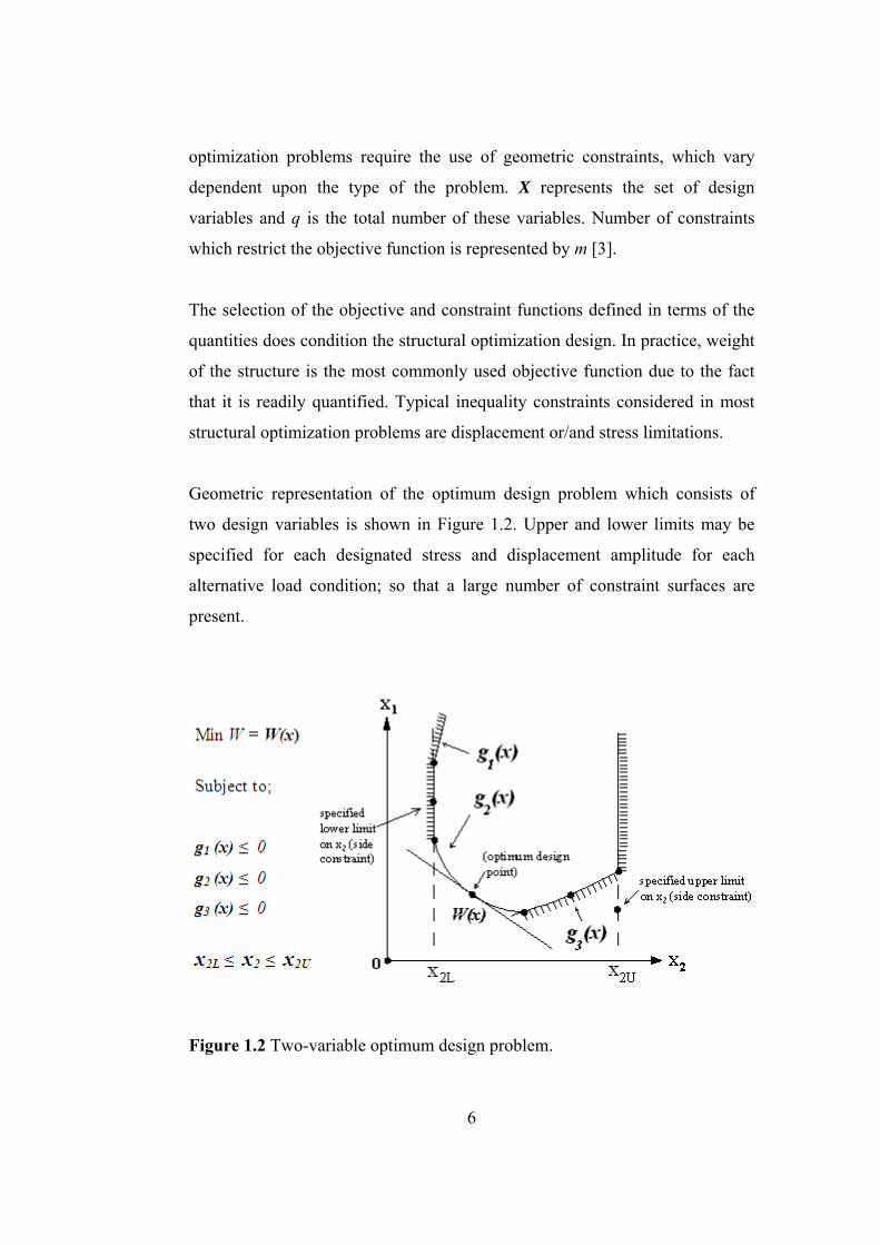
Geometric representation of the optimum design problem which consists of

two design variables is shown in Figure 1.2. Upper and lower limits may be

specified for each designated stress and displacement amplitude for each

alternative load condition; so that a large number of constraint surfaces are

present.

Figure 1.2 Two-variable optimum design problem.

7

Side constraints appear as planes parallel to the coordinate directions when

they refer to minimum or maximum values of the design variables. If a design

point located in the space above the composite constraint surface, it is in free

space and known as a feasible-design or exterior point. Conversely, a design

point that represents the violation of constraints is infeasible or interior. In

geometric terms, Figure 1.2 discloses that the optimum-design problem

consists in finding the optimum design point of the weight and constraint

surfaces [4]. Sometimes optimization problems appear to be unconstrained

problems. At this time, since there are no constraints, all points are feasible and

hence one needs to be concerned only with the value of f (x) at neighboring

points.

1.4.1 Optimization Models

Representation of an optimization problem in a mathematical formulation is a

critical step in the optimization process. Acceptability of a solution for an

optimization problem is dependent upon the correct formulation of three basic

ingredients, namely design variables, objective functions and constraints.

Depending on the problem, models of optimization problems can be divided

into two categories as continuous optimization problems and discrete

optimization problems.

1.4.1.1 Continuous-Variable Models

This model can be stated as an optimization problem which involves variables

for which it is possible to take an intermediate value from an interval of real

8

numbers. For instance, cross-sectional area of a beam and length of an aircraft

wing can be assumed to be variables of two continuous optimization problems.

Continuous optimization can detect branch mis-predictions earlier and thus

reduce the mis-prediction penalty.

1.4.1.2 Discrete-variable Models

Discrete-variable models involve discrete set of variables. These variables

describe a finite set of conditions and take values from a finite, usually small,

set of states. In most of the practical applications of optimization, discrete

variables occur naturally in the formulation of the problem. For instance,

material properties must correspond to the available materials or number of

bolts must be integer.

The distinction between discrete and continuous quantities is rather vague,

while the distinction between discrete and continuous variables is crisp. Many

quantities can be represented as both discrete and continuous. In general,

discrete variables are convenient approximations of real world quantities,

sufficient for the goal of reasoning.

1.4.2 Structural Optimization

In the last three decades a prominent progress has been achieved in the field of

structural analysis. With the help of computer almost all structural problems

can be solved within the limits of human beings’ knowledge of materials.

While these achievements are of the greatest importance in allowing the

9

behavior of a particular design to be assessed, their full benefits for the society

will not be materialized until they are reflected in the improved design of

structures.

The purpose of inventing better design solutions which, while satisfying safety

and performance constraints, do it at least cost, is clearly not a new one. From

the time of earlier history engineers have investigated several alternatives and

chosen the best one of these. Unfortunately, many factors limit severely the

number of alternatives that can be investigated. After the implementation of

computerization to the structural analysis process, it is natural that a

development of more effective and rapid techniques for the search of the

optimum structural design is required.

The optimal design of structures, theoretically, aiming at designing

economical and reliable structures and systems at various conditions and

technological constraints, is an important branch of general science of

optimization.

Much work has been done in the field of structural optimization in recent

years and obviously many techniques exist in the literature. Still, rapid

changes in methods and focus are being witnessed in this relatively new field.

However, there is lack of applications to practical design problems in spite of

the huge amount of literature on the subject. This imbalance is redressed

gradually. These hopeful applications result in the increase in the use of

structural optimization methods to real-life problems.

However, these real-life problems, sometimes, may be so complex that due to

the high computational cost the designers cannot afford to analyze them

several times. Besides, in the analysis of structures most of the designers use

general-purpose software packages such as finite element based commercial

10

software. Generally, the source program of the algorithms cannot be accessed

and the engineers have only scant knowledge of the details of the analysis

programs used in these software packages.

Designers have shown great interest to structural design optimization when it

was first emerged. With the aid of this tool a systematic solution to age-old

structural design problems, handled by utilizing trial-error methods or

engineering intuition or both, is provided.

Traditional algorithms for structural design optimization are usually driven

with deterministic mathematical re-sizing procedures and essentially one

design is replaced through the iteration until a convergence criterion is

reached. These gradient-based and direct algorithms are founded upon a

uniquely human field depicting physical and natural phenomena. Direct and

gradient-based algorithms are powerful search and optimization tools which

can be effectively used in structural optimization problems. Direct

mathematical methods can be described as point-to-point search algorithms

employing objective function and constraints to guide the search through the

feasible design space while gradient-based methods are the algorithms which

utilize derivatives of objective functions and/or constraint equations to guide

the search. Convergence of both methods depends upon the selection of an

initial solution for subsequent modification through iteration and design

variable changes.

Mathematical algorithms are generally problem-specific and the efficiency

and ability of the algorithm in finding the optimum varies. Practical

engineering problems often use discrete design variables such as structural

steel cross-section sizes in building design.

11

The structural optimization problems usually need more than one objective

function, such as, minimum weight which is related to cost, maximum

stiffness, minimum displacement at specific structural points and minimum

structural strain energy provided that the design satisfies all the constraints.

These problems are called as multi-objective optimization problems. For

instance, it is often required that a structure be stiff enough so that the

maximum deflection is within the prescribed limit. The design constraints

provide bonds on member stress, deflection, local buckling, system buckling,

frequency and dynamic response. Since mathematical programming methods

tackle with continuous design variables, the algorithms developed has

provided to designer cross-sectional dimensions that were neither practical nor

standard.

Consequently, from practical point of view the structural design optimization

methods without discrete set of variables cannot be effectively used in real-life

problems. As a result, efforts have been concentrated on the use of discrete

variables in structural optimization algorithms.

1.4.2.1 Structural Optimization Problems

Discrete structural optimization problems can be expressed as finding optimum

values for discrete member design vector x that minimizes the objective

function f (x), which is restricted by the constraints related to the design and

the behavior of the structure. Structural optimization algorithms are generally

formulated to tackle optimization problems whose statements take the

following general form [5];

Find a design vector x, xi X , X = {x1, x2,…, xq}

12

For weight optimization;

(1.5)

Subject to;

(1.6)

(1.7)

(1.8)

Where;

:)(xf the objective function (usually the weight of the structure)

X : table of available discrete size

q : total number of design variables or elements

n : total number of load condition

m : total number of displacement constraints

i : the specific weight of the i-th element

ii xL , : the length and the cross sectional area of the i-th element respectively

:,' aii the absolute value of stress under the l-th load condition and allowable

stress in the i-th element respectively.

13

:,' akk uu the absolute value of displacement under the l-th load condition at the

degree of freedom corresponding to the k-th displacement constraint and

corresponding allowable value respectively.

: the vector of lower bounds on design variables

: the vector of upper bounds on designs variables

The complexity of optimum design problem can vary dramatically depending

on the number of these objective functions, number of constraints and size of

the decision space. In addition, the mapping of decision space to objective

space can lead to increased problem complexity [5].

Structural optimization problems, depending on the geometrical feature, are

divided to three main categories as; sizing optimization, shape optimization,

topology optimization.

1.4.2.1.1 Sizing Optimization Problems

In a simple sizing optimization problem generally cross-sectional areas of each

element are selected as design variables. Structure is optimized by obtaining

the areas of individual elements that minimize the weight or maximize the

stiffness. Sizing optimization is the simplest way of doing structural

optimization. A simple sizing optimization problem for a truss structure is

illustrated in Figure 1.3. [6].

14

a) Initial design b) Optimized design

Figure 1.3 A sizing structural optimization problem.

1.4.2.1.2 Shape Optimization Problems

In the case of shape optimization problem structural design variables represent

the form or contour of some part of the boundary on the structural domain.

Minimization of mass can be leaded by changing or determining boundary

shape while satisfying all design requirements. For over three decades, the

subject of shape optimization has been a topic of in-depth research. It has been

implemented into several commercial finite element programs [5]. Geometric

representation of a two-dimensional shape optimization problem is illustrated

in Figure 1.4 [6] where (x) denotes the shape of the beam-like structure.

Figure 1.4 A shape optimization problem.

F F

15

FF

1.4.2.1.3 Topology Optimization Problems

The topology or “landscape” of the structure must be an outcome of the

procedure. In principle the result of a topology optimization procedure is also

optimal with respect to shape and size, however it should be noted that

fundamental differences in the design parameterization means that direct

comparisons are difficult in practice [5].

Topological optimization of a simple structure can be achieved by considering

cross-sectional areas of members to be design variables, and then allowing

these variables to take the value zero. In other words, bars are removed from

the truss. In this way, the connectivity of nodes becomes variable and the

topology of the structure changes (Figure 1.5.).

a) initial design b) Optimized design

Figure 1.5 Topology optimization of a simple truss.

16

1.4.2.2 Structural Optimization Methods

Optimization theory and methods tackle with selecting the best alternative in

the sense of a given objective function. These methods are perceived to be at

the heart of computer methods for designing engineering systems. With the

help of these methods, the designer can evaluate more alternatives, thus leading

to a better and more cost-effective design. Structural optimization methods can

be categorized as numerical methods and analytical methods. Numerical

methods emphasize the algorithmic aspect, while analytical methods are

concerned with the conceptual aspect.

1.4.2.2.1 Analytical Methods

In the determination of optimum solutions for layouts or geometrical form of

simple structural elements such as beams, columns and plates, analytical

methods usually apply mathematical theory of calculus, variation methods, etc.

They do determine the parameter values of the theoretical model on the basis

of known experimental results. One can easily state that these analytical

methods are most convenient for such fundamental studies of single structural

components. The design of structural systems is represented by a number of

unknown functions and the purpose is to find out the form of these functions.

Theoretical determination of the optimal design is made through the solution of

a system of equations expressing the optimality conditions.

Analytical methods have great importance on the design optimization of

structures. Although they sometimes have insufficiency of the practical aspects

of realistic structures, when they can be found, they provide valuable insight

17

and theoretical lower bound optimum against which more practical designs

may be judged. Structural design optimization problems employing the

analytical methods are known as continuous problems or distributed parameter

optimization problems.

1.4.2.2.2 Numerical Methods

The solution of practical optimization problems, when the number of design

variables is more than two or the constraint functions are complex, is

challenging to obtain with use of closed form analytical solution methods.

Thus, numerical method based algorithms are preferred to solve most structural

optimization problems. These methods employ a branch in the field of

numerical mathematics called mathematical programming. Recent

developments of the numerical methods seem to be result of rapid growths in

computer capacities.

Numerical methods for the structural design optimization problems

conceptually differ from analytical methods described above. In analytical

methods one does write the optimality conditions and solve them for candidate

local optimum designs. However, when numerical methods are used, a

candidate design is selected as an initial estimate for the optimum point and

improved until to further improvements are possible without violating any of

the constraints. The process may require several cycles and number of these

cycles is problem dependent. This iterative formula is acceptable for both

constrained and unconstrained optimization problems.

In summary, the main concept of numerical methods is to start with a

reasonable estimate for the optimal design. Objective and constraint functions

18

are calculated at that point. Based on these evaluations, the design is moved to

a newly generated point. The process is repeated until a stopping criterion is

satisfied. The general algorithm of this iterative scheme can be illustrated as in

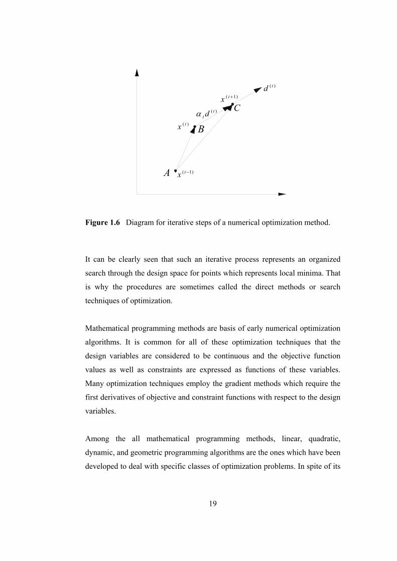
the following, which is also demonstrated graphically in Figure 1.6;

Step 1. Estimate an appropriate candidate design )0(x . Set the iteration counter

t= 0.

Step 2. Calculate a search direction )(td in the design space. This computation

usually requires objective function value and its constraints.

Step 3. Check for convergence of the algorithm. If it has converged, terminate

the process. Otherwise, continue.

Step 4. Compute a positive step size t .

Step 5. Compute the new design as;

)()()1( tt

tt dxx (1.9)

Set 1 tt and go to Step 2.

19

A

B

C

)1( tx

)( tx

)( tt d

)1( tx

)( td

Figure 1.6 Diagram for iterative steps of a numerical optimization method.

It can be clearly seen that such an iterative process represents an organized

search through the design space for points which represents local minima. That

is why the procedures are sometimes called the direct methods or search

techniques of optimization.

Mathematical programming methods are basis of early numerical optimization

algorithms. It is common for all of these optimization techniques that the

design variables are considered to be continuous and the objective function

values as well as constraints are expressed as functions of these variables.

Many optimization techniques employ the gradient methods which require the

first derivatives of objective and constraint functions with respect to the design

variables.

Among the all mathematical programming methods, linear, quadratic,

dynamic, and geometric programming algorithms are the ones which have been

developed to deal with specific classes of optimization problems. In spite of its

20

relatively short history, there have been a large number of optimization

algorithms which employ the mathematical programming.

Another approach for numerical optimization of structures is to derive, from

mathematical considerations, conditions termed optimality criteria which must

be fulfilled by an optimal solution. Although these conditions can be essential

and sufficient for optimality, in most practical design problems, they are only

necessary ones. The most important advantages of this method are that it can

be easily programmed for the computer, it is independent of problem size and

it requires relatively less number of structural analyses.

1.4.2.2.2.1 Mathematical Programming

Mathematical programming approach was first applied to structural

optimization in the late 1950’s. This approach was developed to solve large

problems which have thousands of constraints and variables. Mathematical

programming problems can be divided into two categories as linear

programming and non-linear programming.

Non-linear programming problems, in which higher degrees of any variables

or the reciprocal of the variables may appear, are more general than linear

programming problems. It is developed for non-linear unconstrained

optimization problems. Non-linear programming algorithms necessitate either

gradient or differentiability information of both the objective function and

constraints with respect to the design variables.

The simpler one of these is the linear programming problem, in which the

variables are of first degree. In order to be able to apply linear programming

21

techniques to structural optimization problems, one must express the

relationship between the objective function and the constraints as linear

functions of design variables.

Linear programming problems, in which both objective function and

constraints are linear, can be solved with gradient methods. Algorithm of this

method starts with a feasible solution and proceeds through the direction of the

gradient vector of the objective function until a point on the boundary of the

feasible region is reached. At that point the direction of search is changed

according to certain rules in an iterative manner until the value of the objective

function is the maximum.

The programming methods of calculus of variations, such as the Galerkin

method and the Rayleigh-Ritz method are limited to extremizing an integral

without additional constraints. These methods make use of the approximation

of the free functions by means of finite summations of appropriate known

functions, for which the coefficients of the individual terms are determined,

with the help of ordinary calculus in such a way that the value of the integral in

question becomes a maximum or a minimum.

Kuhn-Tucker conditions and Lagrange equations are necessary conditions for

optimum solutions of non-linear problems. These conditions provide very

basic method for solving non-linear programming problems, although in

practice very few problems can be solved by use of Lagrange equations.

22

1.4.2.2.2.2 Optimality Criteria

The concept of optimality criteria as the basis of selection of a minimum-

volume structure emerged in the early 1960s. This approach derives from the

extremum principles of structural mechanics, and for the most part has been

limited to simple structural forms and loading conditions. Prager and Taylor

have been instrumental in the development of much of this work. The

procedures of Venkayya and Gellatly and Berke are the foremost procedures

of employing this method. A detailed review of these procedures can be found

in [4].

The methods of optimality criteria include two components. The first is the

stipulation of the optimality criteria, which can be rigorous mathematical

statements such as the Kuhn-Tucker conditions, or an intuitive one such as the

stipulation that the strain energy density in the structure is uniform. The

second ingredient is the algorithm used to resize the structure for the purpose

of satisfying the optimality criterion [8].

Methods of optimality criteria assume continuous design variables. In the case

where the discrete variables are considered, a two-step optimality criteria

procedure is used. First, optimum solution is obtained using continuous

variables. Then, using these variables a set of discrete values is estimated. In an

optimum solution procedure where the optimality criteria methods are used, the

design variables represent a single cross- sectional property of a structural

member. A number of functions of the selected design variable express all

other cross-sectional properties of this member.

23

1.4.3 Stochastic Search Methods

Optimization problems in practice depend mostly on several model parameters,

noise factors, uncontrollable parameters, etc., which are not given fixed

quantities at the planning stage. Typical examples from engineering and

economics/operations research are; Material parameters (e.g. modulus of

elasticity, yield stresses, allowable stresses, moment capacities, specific

gravity), external loadings, friction coefficients, moments of inertia, length of

links, manufacturing errors, tolerances, noise terms, demand parameters,

technological coefficients in input-output functions, cost factors, etc.. Due to

several types of stochastic uncertainties (physical uncertainty, economic

uncertainty, statistical uncertainty, and model uncertainty) these parameters

must be modeled by random variables having a certain probability distribution.

In order to cope with these uncertainties, instead of relying on ordinary

deterministic parameter optimization methods, stochastic search methods are

applied [9].

Some of the optimization algorithms developed recently employ stochastic

optimization methods in which random numbers are generated. Stochastic

search methods do not require the evaluation of the gradients of the objective

and constraint functions; however, they require more function evaluations. An

advantage of these algorithms to nonlinear algorithms is that they can be

applied to optimization problems involving discrete variables.

24

1.4.3.1 Genetic Algorithms

Genetic algorithms are stochastic search techniques on the basis of the

mechanism of natural selection as well as natural genetics and rely on the

principle of Darwin’s theory of survival of the fittest. Algorithms were first

introduced by John Holland in the 1960s and developed by Holland, his

students and colleagues in the 1960s and the 1970s [10].

Genetic algorithm routine starts with an initial set of random solutions called

population. This population includes some individuals called chromosomes,

representing a solution to the problem. Each chromosome is a string of

symbols, which is usually a binary bit string. A positive value, generally called

fitness value, is used to reflect the degree of “goodness” of the chromosome for

the problem which would be highly related with its objective value.

The initial population is set by constructing each chromosome where all the

variables are in a binary coded form. Each character in this code can take either

the symbol of ‘0’ or ‘1’. After the decoding process, the fitness of each

solution string is evaluated. Throughout a genetic evolution, the fitter

chromosome tends to yield good quality offspring which means a better

solution to any problem. In each cycle of genetic operation, termed as an

evolving process, a subsequent generation is created from the chromosomes in

the current population. This can only succeed if a group of these chromosomes,

generally called “parents” or a collection term “mating pool” is selected via a

specific selection routine. The genes of the parents are mixed and recombined

for the production of offspring in the next generation. It is expected that from

this process of evaluation (manipulation of genes), the “better” chromosome

will create a larger number of offspring, and thus has a higher chance of

surviving in the subsequent generation, emulating the survival-of-the-fittest

25

mechanism in nature [10]. The cycle of evolution is repeated until a desired

termination criterion is reached. This criterion can also be set by the number of

evolution cycles, or the amount of variation of individuals between different

generations, or a pre-defined value of fitness.

1.4.3.2 Tabu Search

The philosophy of tabu search is to derive and exploit a collection of principles

of intelligent problem solving. In this sense, it can be said that tabu search is

based on selected concepts that unite the fields of artificial intelligence and

optimization. The basic form of tabu search is founded on the ideas proposed

by Fred Glover [11]. The method is based on the procedures designed to cross

boundaries of feasibility or local optimality, which were usually treated as

barriers. It is an iterative improvement procedure that starts from any initial

solution and attempts to determine a better solution.

The algorithm begins by marching to a local minimum. To avoid retracing the

steps used, the method records recent moves in one or more tabu lists. The

original intent of the list was not to prevent a previous move from being

repeated, but rather to insure it was not reversed. The tabu lists are historical in

nature and form the tabu search memory. The role of the memory can change

as the algorithm proceeds.

Algorithm is initialized with the random construction of initial design which is

considered as the current solution. Design variables are then selected and a

number of candidate designs are created considering the neighborhood of the

current solution. All the candidate solutions are analyzed and objective

function values are calculated. The one which has the lowest value is

26

determined and stored as the best candidate. It is checked if the best candidate

is forbidden or not. If it is not forbidden then the candidate design is replaced

by current solution, and the design is accepted and recorded in the tabu list. If

a prohibited candidate satisfies the aspiration criterion, it replaces the current

solution and tabu list is revised. If not the candidate design is not accepted and

the search is carried on with the current design. Once all the design variables

are selected, a single iteration is completed. This procedure is repeated until

the predefined number of generations is completed.

1.4.3.3 Evaluation Strategies

Evolution strategies is an optimization technique developed in 1963 [12]. The

strategy performs well in domains where it is impossible, difficult or

expensive to define a precise mathematical description of the problem at hand.

The method deals with vectors of real numbers for the representation of

designs and optimization parameters. It is very similar to genetic algorithms.

The main differences between evolutionary strategies and the genetic

algorithms are the method of selection and whether the sensible strategy

parameters are adjusted or not. Moreover, only the best fit individuals are

allowed to reproduce in the evolution strategies method. Steps of the algorithm

can be summarized as follows;

Algorithm is initialized generating a number of parent individuals to construct

the initial population. Each individual in the initial population is evaluated.

Parent population then undergoes recombination and mutation operators to

yield the offspring population. With recombination, a trade of design

information between the parents is provided to generate new individuals.

Mutation, on the other hand, is the main operator of evolution strategies. It is

27

based on a normal distribution requiring the mean ξ and the standard deviation

σ. In order to determine the survivors out of parent and offspring populations,

selection should be implemented. The selected individuals become the parents

of the next generations. This procedure is repeated until the predefined

number of generations is completed.

1.4.3.4 Simulated Annealing

The simulated annealing is a random-search technique which utilizes an

analogy between the way where a metal cools and freezes into a minimum

energy crystalline structure (the annealing process) and the search for a

minimum in a more general system; it forms the basis of an optimum design

method for combinatorial and other problems.

The algorithm was developed in 1983 [12] to be able to solve highly nonlinear

problems. The behavior of the algorithm is similar to solidification of metals or

formation of crystals. The achievement of a number of solid states with

different internal atomic or crystalline structure that correspond to different

energy levels depends on the rate of cooling. If the cooling is too rapid, it is

most likely that the resulting solid state would have a solid margin of stability

because the atoms will assume relative positions in the lattice structure to reach

an energy state which is only locally minimal. In order to obtain a more stable,

globally minimum energy state, the annealing process is used where the metal

is reheated to a high temperature and cooled slowly; letting the atoms enough

time to find positions that minimize a steady state is reached.

The major advantage of the algorithm is an ability to avoid becoming trapped

in local minima. Random search employed by simulated annealing accepts not

28

only changes that decrease the objective function value f (assuming a

minimization problem), but also some changes that increase it. The cooling

schedule is the main process of the algorithm. The cooling schedule of a

simulated annealing algorithm involves four components as; starting

temperature, final temperature, temperature reduction, iterations at each

temperature.

Algorithm starts with a certain temperature value. It must be hot enough to

allow a move to almost any neighborhood state. If it is not hot enough then the

ending solution may be the same (or very close) with the starting solution.

However, if the initial temperature is too high then the search can move to any

neighbor and thus convert the search (at least in the early stages) into a random

search. It is usual to allow the temperature decrease until its final value reaches

zero. In practice, however, it is not essential to let the temperature reach zero

because as it approaches to zero the possibility of accepting a worse design is

almost the same as the temperature being equal to zero. To make the final

temperature equal or close to zero a temperature reduction is needed. This is

done by using simple linear method or geometric decrement method. Another

important factor is the number of iterations at each temperature. A constant

number of iteration at each temperature is a common scheme.

.

1.4.3.5 Ant Colony Optimization

The ant colony optimization is a meta-heuristic search technique which is used

to find optimum solutions for combinatorial optimization problems, which is

inspired by the foraging behavior of the social insects. The algorithm belongs

to the class of model-based search algorithm. These types of algorithms are

characterized by the probabilistic model which is used to generate solutions to

29

the optimization problem. Ant colony optimization algorithms use a given

probabilistic model without changing the model structure during run-time.

Real ants have the capability of finding the shortest path from food to their

nests. They can also adapt to changes in the environment, for instance, finding

a new shortest path if the old one is no longer available. They can do this with

the help of pheromone trails, which ants use to communicate information

among individuals regarding the walking path or the decision about where to

go. Once an ant finds a food source, it brings some of the food to the nest. It

releases a pheromone trail on the ground while it is walking. Other ants find

the food source following this pheromone trails deposited on the ground. Each

ant would rather follow a direction rich in pheromone. They find the shortest

path between their nest and the food sources with the help of this indirect

communication [12], which is demonstrated in Figure 1.7.

Figure 1.7 Path which is designed by ants to reach the destination.

Ant colony algorithm can be summarized as follows: A set of agents, a colony

of ants, moves through states of the problem corresponding to partial solutions

of the optimization problem. They apply a stochastic local decision policy to

Source

Destination

30

move. The trails and attractiveness are two parameters of the algorithm, which

are the basis of this policy. By moving, each ant incrementally forms a solution

to the problem. When an ant reaches to the destination .i.e. completes a

solution, or during the construction phase, the ant evaluates the solution and

modifies the trail value on the components used in its solution. This pheromone

information will direct the search of the future ants [13]. The skeleton of ant

colony optimization algorithm includes three major phases, namely, the

initialization phase, the solution construction phase and pheromone updating

phase.

In the initialization phase first the pheromone trail strength for all the edges is

initialized. Then the number of artificial ants in a colony is set and each ant is

put on a randomly chosen vertex. Afterwards, the termination criteria for the

iteration looping are set up, which may be that the iteration number exceeds

the predefined number of solution construction steps or that the computation

time has exceeded a given CPU-time limit. Secondly, the solution construction

phase starts. At the beginning of this phase, ants have already been put on

randomly chosen vertices on the construction graph, and their paths consist of

their initial vertices. In each construction step, all the ants arrange their

feasible paths by moving to the next vertex based on the probabilistic decision

according to the transition rule. After all the ants have moved once, their

current feasible paths may be improved by applying local pheromone updating

rule. When all the ants have completed their feasible paths, the solution

construction phase is stopped. Then the pheromone trails are updated using

global pheromone updating rule.

31

1.4.3.6 Harmony Search Algorithm

Harmony search optimization is a stochastic optimization technique developed

by Geem and Kim [14]. It is relatively simple method which imposes fewer

mathematical requirements for the solution of optimization problems. It

requires neither initial starting values for the decision variables nor the

derivative information of the objective function and constraints. Therefore, it is

easy to program harmony search method. As in the nature of stochastic

optimization methods, harmony search algorithm starts with randomly selected

candidate solutions to the optimization problem from a solution set. Feasible

ones amongst all are selected and a harmony search memory in which each

candidate solution is stored in descending order is constructed. Then the

procedure is followed by filling the harmony memory matrix with new

solutions depending on the parameters called the harmony memory considering

rate and the pitch adjusting rate.

The idea behind the algorithm is found in the paradigm of natural phenomena.

Harmony search algorithm, belonging to the class of meta-heuristic algorithms

that seek a stable state, drives its roots in the harmony of a musical

performance. In other words, it imitates the musical improvisation process in

which the musicians search for the best harmony. Music harmony may be

defined as a combination of sounds considered pleasing from an aesthetic point

of view. For example, during jazz operation, jazz improvisation tries to obtain

musically pleasing harmony as determined by an aesthetic standard. It is

similar to an optimization process that seeks to find an optimum solution. The

aesthetic quality is determined by the pitch of each musical instrument just as

the set of values assigned to each design variable define the objective function

value. Musicians can improve the sounds for better quality through practice

32

after practice, similarly, design values for better objective function evaluation

can be improved iteration by iteration [15].

Algorithm starts with the specification of harmony search algorithm parameters

(harmony memory size, harmony memory considering rate, pitch adjusting

rate, number of objective function evaluations). Harmony memory is filled

with as many randomly generated solution vectors as the size of the harmony

memory. New harmony vector is then improvised by three rules as random

selection, harmony memory consideration and pitch adjustment. If the new

harmony vector is better than the worst harmony in the harmony memory, the

new harmony and the existing worst harmony are replaced. This procedure is

repeated until the predefined number of improvisation is reached.

1.4.3.7 Big bang- big crunch Optimization

The big bang-big crunch optimization method is a recent addition to meta-

heuristic optimization techniques. This new optimization method is developed

by Erol and Eksin [16] which has a low computational time and high

convergence speed. The basic idea behind the algorithm is the theory of the

evolution of the universe. Algorithm is divided into two main steps: The first is

the big bang phase and the second step is the big crunch. In the former step,

energy dissipation produces disorder and randomness just as in optimization

method candidate solutions are randomly generated and distributed over the

search space. In the big crunch step, randomly distributed particles are drawn

into an order just as the optimization method a center of mass for the

population is calculated by a contraction procedure. That is, the contraction

operator takes the current positions of each candidate solution in the population

and its associated objective function value and computes a center of mass. The

33

term mass refers to the inverse of the objective function value. After the big

crunch phase, new positions of candidate solutions are generated using the

center of mass.

These successive explosion and contraction phases are carried out repeatedly

until maximum number of iterations has been met. The steps of the big bang-

big crunch optimization method can be summarized as follows;

1) Big bang phase: Initial candidate solutions are randomly generated in

the search space.

2) Objective function value of each candidate solution is calculated.

3) Center of the mass is determined.

4) Using center of the mass calculated in previous step new candidate

solutions are obtained.

5) Step 2- 4 are repeated until termination criterion is satisfied.

1.4.3.8 Particle Swarm Optimization

Particle Swarm Optimization technique was firstly developed by Kennedy and

Eberhart and has been used for various optimization fields [17]. It is a

numerical optimization technique that simulates the social behavior of birds,

fishes and bugs. In nature fish school, birds flock and bugs swarm not only for

reproduction but for other reasons such as finding food and escaping

predators. Similar to birds seek to find food, the optimum design process seeks

to find the optimum solution. Each individual is called particle and whole

34

population is named as swarm. In the particle swarm optimization, each

particle in the swarm represents a candidate solution of the optimum design

problem.

Experiments show that the particle swarm method is an efficient and robust

technique in finding the optimum solution [18-27].

In this study, optimum design of semi-rigid steel frames including soil structure

interaction is determined by using particle swarm algorithm. This technique is

discussed in detail in Chapter 2.

1.4.4 Constraint Handling Methods

There exist several ways of incorporating the constraints into the fitness

function available in the literature [28]. Amongst all, penalty functions have

been the most common way of incorporating constraints into meta-heuristic

search techniques. One recent addition to these techniques is fly- back

mechanism. The constraint handling methods work in a search space involving

feasible and infeasible sub-spaces as illustrated in Figure 1.8.

35

Infeasible space

feasible space

global minimum

Figure 1.8 Global minimum in the feasible space.

1.4.4.1 Penalty Functions Method

In the literature, the penalty functions approach has been employed in

conjunction with all meta- heuristic search techniques. This approach was

originally proposed in the 1940s [28]. The main concept of this method is

transforming a constrained- design optimization problem into an unconstrained

one by adding or subtracting a certain value to/from the objective function

value based on the amount of constraint violation present in a certain solution.

There are two kinds of penalty functions considered in classical optimization

called exterior and interior methods. While employing the exterior methods,

the process is initialized with an infeasible solution and let move towards the

feasible region. In the case of latter methods, the penalty term is determined in

such a way that its value will be small at points away from the constraint

boundaries and will tend to be infinite as the constraint boundaries are

36

approached. Then, if starting point is feasible, the points generated

subsequently will always lie within the feasible region. In most of the

optimization problems, exterior penalty functions method is used due to the

fact that this method does not require an initial feasible design. The

formulation of exterior penalty functions method is given as follows;

p

jjj

n

iii LcGrxfx

11

..)()( (1.10)

In which, )(x is the expanded objective function to be optimized, iG and jL

are the constraint functions and ir and jc are the constants called penalty

factors. iG and jL is generally defined as in the following form;

Gi = max [ 0, gi (x) β ]

)(xhL jj (1.11)

Where; )(gi x and )(xhj are the constraints, and are generally 1 or 2.

Ideally, the penalty should be kept as low as possible, just above the limit

below which infeasible solutions are optimal. This is due to the fact that if the

penalty is too high or too low, then the problem might become very difficult. If

the penalty is too high and the optimum lies at the boundary of the feasible

region, the process will be pushed inside the feasible region very quickly, and

will not be able to move back towards the boundary with the infeasible region.

A large penalty discourages the exploration of the infeasible region since the

37

very beginning of the search process. On the other hand, if the penalty is too

low, a lot of the search time will be spent exploring the infeasible region

because the penalty will be negligible with respect to the objective function.

These issues are very important in optimization algorithms, because many of

the problems in which they are used have their optimum lying on the boundary

of the feasible region. It is known that the relationship between an infeasible

individual and the feasible region of the search space plays a significant role in

penalizing such an individual [28].

Several researchers have studied heuristics on the design of penalty functions,

one of which has the following guidelines [28]:

1) Penalties which are functions of the distance from feasibility are better

performers than those which are only functions of the number of violated

constraints.

2) For a problem having few constraints, and few feasible solutions, penalties

which are solely functions of the number of violated constraints are not

likely to produce any solutions.

3) Good penalty functions can be constructed from two quantities: the

maximum completion cost and the expected completion cost. The

completion cost refers to the distance to feasibility.

4) Penalties should be close to the expected completion cost, but should not

frequently fall below it. The more accurate the penalty, the better will be

the solution found. When a penalty often underestimates the completion

cost, then the search may fail to find a solution.

38

1.4.4.2 Fly-back Mechanism

This method was first proposed to handle the constraints of the optimization

problems employing particle swarm optimization technique. The intuitive idea

to maintain a feasible population is for a design point to fly back to its previous

position when it is outside the feasible region. This is the so called ‘fly-back

mechanism’. The technique starts from a feasible initial population. A closed

set of operators is used to maintain the feasibility of the solutions. If new

design violates the constraints then previous design is returned. Therefore, the

subsequent solutions generated at each iteration are also feasible. Algorithms

based on this technique are much more reliable than those based on a penalty

approach [22].

1.5 Literature Survey

The studies and the algorithms developed in recent years for the particle swarm

algorithm, optimum design of rigid and semi-rigid steel frames and the analysis of

soil-structure interaction can be reviewed in a historical order as follows;

Particle swarm optimization technique [17-27] is originally formulated as a

continuous optimization method, which is first introduced by Kennedy and

Eberhart [18]. Continuous applications of this algorithm have been reported in

He et al. [22]. Tasgetiren et al. [23] and Arumugam et al [25] have been the

first researchers using binary numbers in particle swarm optimization to

achieve discrete set. Liu et al. [24] used rounding off method in their research.

A few studies in the literature, such as Li et al. [26], focused on improving the

performance of particle swarm algorithm developed for solution of structural

39

optimization problems. Kaveh and Talatahari [27] increased the performance

of particle swarm optimizer by hybridizing it with ant colony optimization

algorithm.

Khan [29] and Saka and Kameshki [33] used optimality criteria for the

optimum design of steel frames. Camp et al. [31] and Saka and Kameshki [34]

used genetic algorithms to optimize the weight of framed structures. Huang

and Arora [32], Park and Sung [35] employed SA in the optimum design of

steel plane frames subjected to design constraints of American Institute of Steel

Construction-Manual of steel construction: allowable stress design (AISC-

ASD) [30]. An ant colony optimization based optimum design algorithm is

developed for the design of steel frames by Camp et al. [36]. Degertekin [37]

applied SA and GAs to the optimum design of geometrically non-linear steel

space frames. Saka has presented an extensive review for the optimum design

of steel frames in [38]. Recently, Dogan and Saka [39] carried out the particle

swarm method based optimum design of steel frames with rigid end

connections.

Chen and Kishi tackled the modeling of semi-rigid connections of steel frames

in [40]. Hsieh and Deierlein [41] and Xu [42] dealt with the analysis of steel

frames with semi-rigid connections. Hadianfard and Razani [43] considered the

effects of semi-rigid behavior of the connections in the finite element analysis

and in the reliability analysis of steel frames. Various algorithms developed for

the optimum design of steel frames with semi-rigid connections have been

presented in [44-47]. Recently, Dogan and Saka [48] developed a particle

swarm method based optimum design algorithm for partially restrained steel

frames subjected to design constraints of American Institute of Steel

Construction-Manual of steel construction: load and resistance factor design

(LRFD-AISC) [49].

40

Literature in the soil-structure interaction area is rather extensive. Finite and

boundary element methods and spring models [50-59] are the main approaches

used to represent the soil media. Lysmer and Kuhlemeyer [53], Godbole et al.

[54], Rizos [55] and Park et al. [56] are the ones dealing with the finite element

and boundary element approaches. Vesic [58] and Allam and Subba [59] used

this approach in their researches. Soil media can be represented using spring

models, as presented in [57]. Dutta and Roy presented an extensive review for

the modeling of soil-structure interaction in this study.

1.6 Scope of Work

This thesis is concerned with optimum design of semi-rigid steel frames

including soil-structure interaction, in which the optimum design algorithm is

based on the particle swarm optimization method. The organization of the

thesis is as in the following: In the first chapter, a brief introduction is given to

semi-rigid steel frames, soil-structure interaction, optimization, structural

optimization, an overview on existing structural optimization methods. In

chapter 2, the fundamentals of particle swarm algorithm and the basis of the

algorithm what is called swarm intelligence are discussed. In the last part of

the chapter, numerical test problems available in the literature are solved by

using particle swarm algorithm and the results are compared with those of

other optimization techniques. Chapter 3 contains explanation of rigidly

connected steel sway (moment resisting) frames, design of steel frames to

LRFD, structural optimization of steel frames including the definition and

selections of design variables. Several steel frames are optimized using

particle swarm optimization and optimum designs are compared with the ones

obtained with other stochastic optimization methods. In Chapter 4, semi-rigid

41

steel frames are carried out, design of such frames to LRFD is formulated,

particle swarm optimization based optimum design algorithm is introduced

and a number of semi-rigid steel frame examples are optimized with optimum

design algorithm developed. Chapter 5 is devoted to the consideration of soil-

structure interaction in the analysis and design of rigid and semi-rigid steel

frames. In sixth and the last chapter, some brief discussions and conclusions

are presented.

42

CHAPTER 2

PARTICLE SWARM ALGORITHM

2.1 Introduction

The particle swarm optimization method is one of the stochastic random search

methods that is developed by Eberhart and Kennedy in 1995 [18], inspired by

social behavior of bird flocking or fish schooling. This behavior is concerned

with grouping by social forces that depend on both the memory of each

individual as well as the knowledge gained by the swarm. The phenomenon

behind this behavior is called swarm intelligence. Besides, the particle swarm

optimization is also related to evolutionary computation, and has some

common features with genetic algorithm and evolutionary strategies.

2.1.1 Swarm Intelligence

The basic definition of intelligence can be pointed out as; a word that is usually

used to describe the mental abilities of humans, although it can be applied to

other organisms and even to inanimate things such as computers. Collection of

these agents that interact with one another is called swarm. Researchers have

discovered that behavior of swarm is different from that of individual itself.

Swarm intelligence, which is first used as an expression by Hackwood and

43

Wang [60] in the context of cellular robotic systems, is the discipline focuses

on the collective behaviors that result from the local interactions of the

individuals with each other and with their environment. Examples of systems

studied by swarm intelligence are colonies of ants and termites, schools of fish,

flocks of birds, herds of land animals. Some of them are illustrated in Figure

2.1.

a)

b)

c)

Figure 2.1 Examples of swarm intelligence found in the nature a) Bird

flocking, b) Fish schooling, c) Animal herding (http://www.cs4fn.org/

optimization/swarmintelligence.php).

44

Swarm intelligence has some basic principles. The first, the proximity

principle, means that swarm should be able to do elementary space and time

computations. Because space and time translate into energy expenditure, the

swarm should have some ability to compute the utility of a given response to

the environment in these terms. Despite the kinds of activity may vary greatly,

depending on both the type and complexity of the organisms, some typical

activities consist of the search and retrieval of food, the building of nests,

defense of the swarm, collective movement, and in the case of higher

organisms, the interaction necessary for many social functions. Second is the

quality principle: The swarm should be capable of responding not only to time

and space considerations but to quality factors such as the quality of foodstuffs

or safety of location. Third principle is the principle of diverse response which

means that the swarm should not allot all of its resource along consumedly

narrow lines. Resources should be distributed along many modes as insurance

against the sudden change in any one of them. The last principle is the

principle of stability where it is declared that the swarm should not change its

behavior from one mode to another upon every fluctuation of the environment,

since such changes take energy and may not produce a worthwhile return for

the investment [61].

2.1.2 Evolutionary Computation

Mind and evolution are known as the two great stochastic systems in nature.

These systems have provided some of the most exciting challenges in the

history of computer science. Modeling the information-processing methods of

minds was the task of the artificial intelligence movement. Evolutionary

computation, subfield of artificial intelligence, uses iterative progress, such as

growth or development in a population. This population is then chosen in a

45

guided random search using parallel processing to obtain the desired end. Such

processes are often inspired by biological mechanisms of evolution.

Evolutionary computing paradigms are closely related to the swarm methods.

These paradigms provide tools to built intelligent systems that model

intelligent behavior. Evolutionary computation is divided into four areas as;

genetic algorithms, evolutionary programming, evolution strategies, genetic

programming. Particle swarm algorithm has some common features with these

areas. For example, particle swarm algorithm is similar to evolutionary

programming, in which each population member is mutated to produce a

candidate population member for the next generation. In addition, in both

evolutionary strategies and particle swarm optimization, one parent can

produce only one child. Moreover, particle swarm algorithm and genetic

algorithms are similar in that the system is initialized with a population of

random solutions.

2.2 Particle Swarm Algorithm

Based on the natural phenomena emphasized above, the particle swarm

optimization technique is developed to deal with many optimization problems

in engineering. It is pretty simple mathematically, and has been applied to a

wide range of problems in several different areas [17-27]. It can be thought of

as a process whereby particles move in n-dimensional space, each particle

being a solution and the space being the problem. Particle swarm algorithm

defines three properties, one of which is velocity which directs movement

throughout the problem space, and the rest of which are particle’s best and

global best which are communicated throughout the swarm. Particle’s best

represents the fitness of each solution so far and global best represents global

46

fitness of each solution as it passes through the problem space. Particles follow

the neighboring optimum particles by adapting these properties in each

iteration or generation.

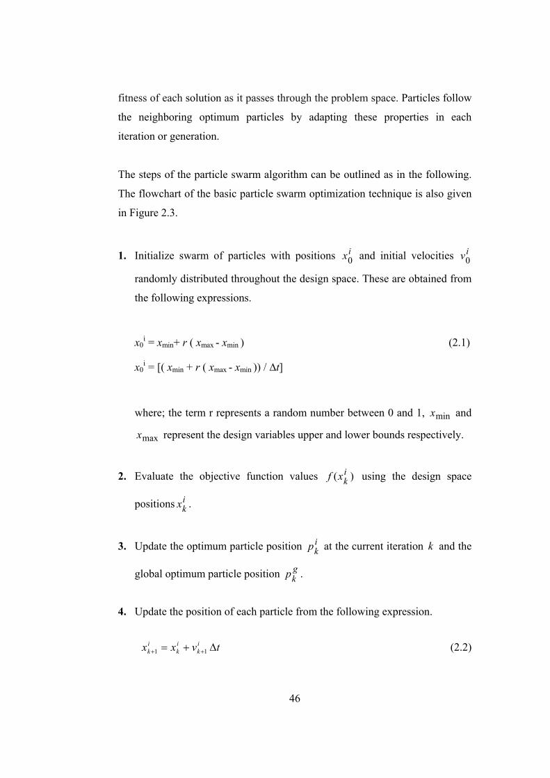
The steps of the particle swarm algorithm can be outlined as in the following.

The flowchart of the basic particle swarm optimization technique is also given

in Figure 2.3.

1. Initialize swarm of particles with positions ix0 and initial velocities iv0

randomly distributed throughout the design space. These are obtained from

the following expressions.

x0i = xmin+ r ( xmax - xmin ) (2.1)

x0i = [( xmin + r ( xmax - xmin )) / ∆t]

where; the term r represents a random number between 0 and 1, minx and

maxx represent the design variables upper and lower bounds respectively.

2. Evaluate the objective function values )( ikxf using the design space

positions ikx .

3. Update the optimum particle position ikp at the current iteration k and the

global optimum particle position gkp .

4. Update the position of each particle from the following expression.

tvxx ik

ik

ik 11 (2.2)

47

Where; ikx 1 is the position of particle i at iteration 1k , i

kv 1 is the

corresponding velocity vector and t is the time step value.

5. Update the velocity vector of each particle. There are several formulas for

this depending on the particular particle swarm optimizer under

consideration. The one has the following form.

(2.3)

Where; r1 and r2 are random numbers between 0 and 1, pki is the best position

found by particle i so far, and pkg is the best position in the swarm at time k.

w is the inertia of the particle which controls the exploration properties of the

algorithm. c1 and c2 are the trust parameters. This expression is also shown

schematically in Figure 2.2.

Figure 2.2 Demonstration of an update in the velocity vector of a particle.

48

Figure 2.3 Flowchart of the basic particle swarm algorithm.

Start

Select number of particles = N

Randomly initialize all the particles’ positions ( xi ) in the range of [ Xmin , Xmax ]

Evaluate fj

İf fj is better than Pbesti then Pbesti = fj

Gbest = Best of Pbesti

Update velocity ( Vi ) of jth particle

xi = xi + (Vi) t

t < itmax

Stop

Yes

No

t = t + 1

Optimum solution = Gbest

Pbesti = fj

Xmin : Lower bound of the set Xmax : Upper bound of the set t : Cycle number itmax : Total cycle number Vmax : Maximum velocity xi : Particle’s position

t : time step

Randomly initialize all the particles’ velocities ( Vi ) in the

range of [ -Vmax , Vmax ]

49

2.2.1 Inertia Weight

The inertia weight can be defined as a scaling factor associated with the

velocity during the previous time step, resulting in a new velocity update

equation. In other words, it is employed to control the impact of the previous

history of velocities on the current velocity thereby, influencing the trade-off

between global and local exploration abilities of the flying points. If larger

inertia weight is selected then global exploration is facilitated, whereas a

smaller inertia weight tends to facilitate local exploration. Suitable selection of

inertia weight parameter makes it possible to have a balance between global

and local exploration abilities and therefore optimization process requires less

iteration to find the optimum.

2.2.2 Control Parameters

The control parameter, sometimes called acceleration constant, is very

important in determining the type of the path that particle travels. If selected

value is very small then the trajectory rises and falls slowly over time.

Specifically, 1c indicates how much confidence the particle has in itself

whereas 2c indicates how much confidence the particle has in the swarm.

2.2.3 Vmax

The particle swarm algorithm involves the modification of the distance that

each particle moves on each dimension per iteration. Velocity changes in a

50

stochastic manner and if the result of this change is undesirable the particle’s

trajectory can expand into wider cycles through the problem space, eventually

approaching infinity. A traditional method to reduce the oscillations is to

restrict the velocity of the particle with a constant value called system

parameter, a representation of which is illustrated as;

maxmax vvthenvv ii (2.4)

maxmax vvthenvv ii

The system parameter Vmax has an important effect of preventing explosion

and adjusts the exploration of the particle’s search. It would be better to take

smaller values in approaching an optimum.

2.2.4 Neighborhood Topology

An important feature of the particle swarm optimization algorithm is that the

fitness information is shared with individuals in a particle’s neighborhood. The

robustness of the algorithm comes from the interactions of particles with their

neighbors. As one particle explores a local optimum, it becomes the best in its

neighbors’ neighborhoods and they too attracted to the optimal region. As the

particles move toward the new optimum, their search may uncover new regions

which are even better, and they may end up attracting the firdt particle toward

their best positions, and so on. The kind of neighborhood structure used affects

the rate at which information is disseminated throughout the population.

There are two types of neighborhoods in which the particles have been studied;

gbest and lbest. In the gbest neighborhood each particle is attracted to the best

51

solution found by any member of the swarm. This structure becomes

equivalent to a fully connected network where each member of the swarm is

able to compare the performances of every other member of the population,

mimicing the very best. In the lbest network, on the other hand, each individual

is affected by the best of its immediate neighbors. The selection of social

structure used has been a matter of artistry with little data to help the researcher

decide a strategy. It is determined that gbest neighborhood tends to converge

more rapidly on optimum than lbest population, but are also more convenient

to converge on local optimum. In Figure 2.4 three different neighborhood

topologies are illustrated. In the star topology, every particle can communicate

with every other particle and is attracted to the global best solution. In the ring

(circle) topology, individuals which are distant from one another are also

independent of one another, however neighbors are closely connected. The

wheel topology, on the other hand, isolates individuals from one another, as all

information has to be communicated through the focal individual. This focal

individual compares all the individuals in the swarm and adjusts its trajectory

through the best of them. Present study uses this type of neighborhood

topology.

a) b) c)

Figure 2.4 Different neighborhood topologies: a) Star topology used in gbest;

b) Ring topology used in lbest; c) Wheel topology (Focal)

52

2.3 Particle Swarm Optimization in Continuous Design Space

Continuous optimization can be defined as the study of the problems where it

is demanded to optimize a continuous function in which the variables take the

values from real numbers. In real number space, the parameters of a function

conceived as a point in multidimensional space. From this point of view,

change over time is represented as movement of the points or particles.

Particle swarm optimization algorithm is originally developed as a continuous

optimization method. It has been implemented to various optimization

problems in real-number space and proved that it is simple to use, robust and it

converges rapidly.

2.3.1 Numerical Examples in Continuous Design Space

The particle swarm optimization method described in the previous sections is

used to determine the optimum solutions of number of continuous optimization

problems. Fly-back mechanism, a powerful constraint handling technique

described in previous chapter, is used in each example.
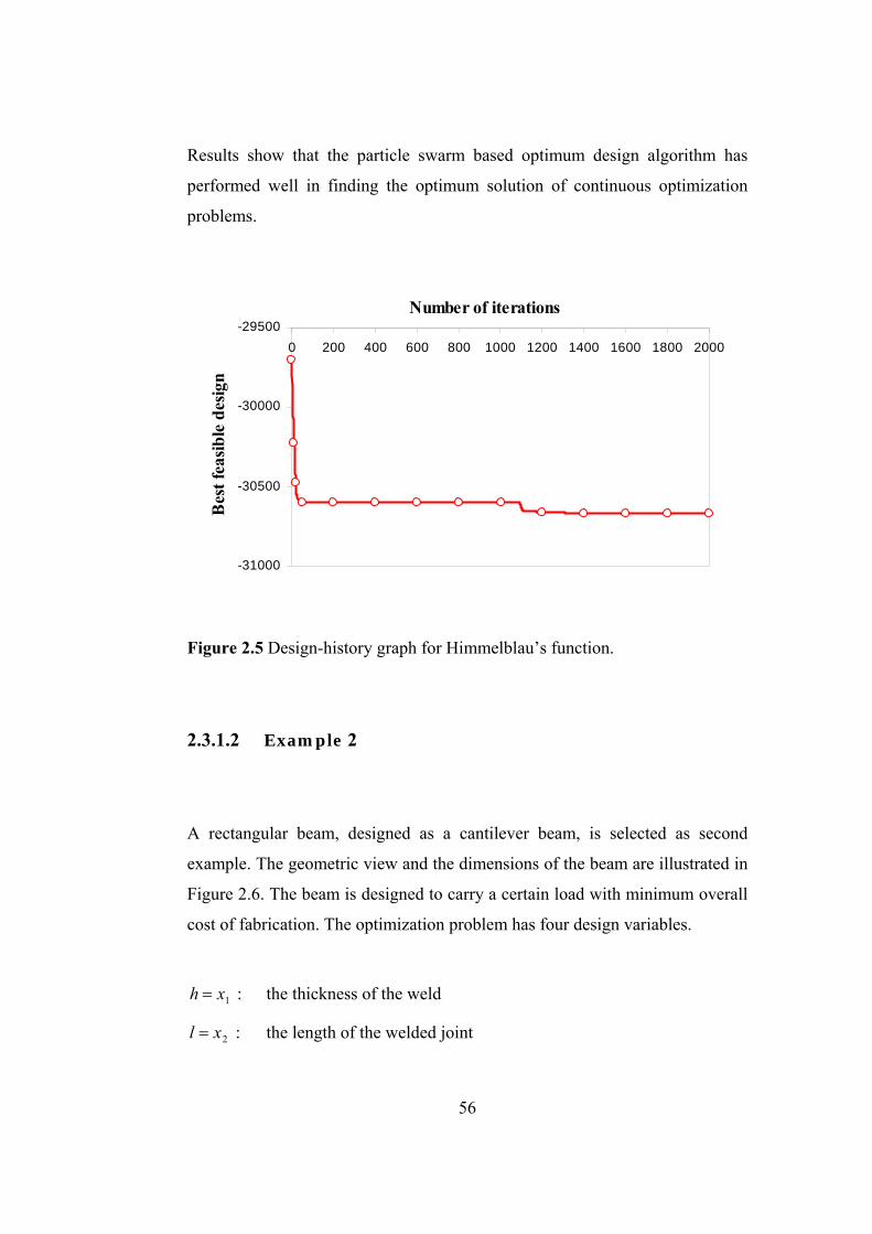
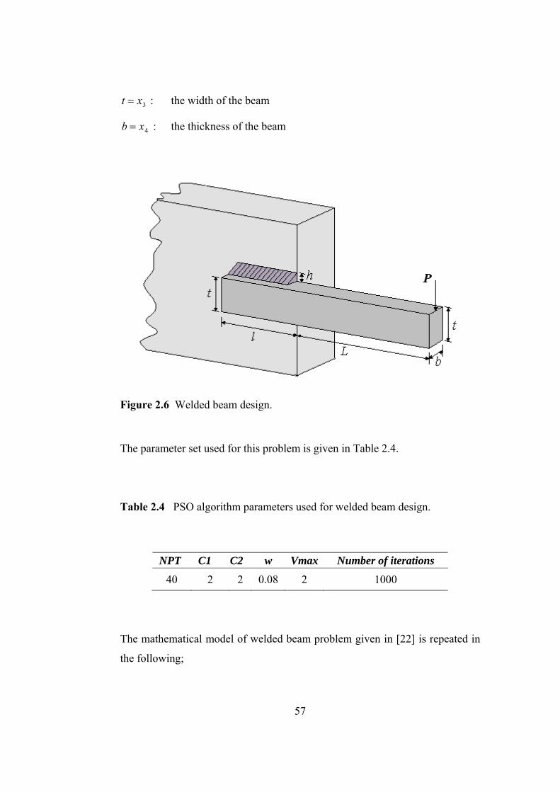
2.3.1.1 Example 1

The first problem, called Himmelblau’s function [62], is a commonly used

benchmark function for nonlinear constrained optimization problems. This

problem is adopted to test the performance of the particle swarm optimization

53

algorithm. Problem has five design variables and fifteen constraints. Problem

definition and optimum design results are as in the following;

Minimize;

141.40792293239.378356891.03578547.5)( 15123 xxxxxf (2.5)

Subject to;

25)(20

110)(90

92)(0

3

2

1

xg

xg

xg

(2.6)

and side constraints;

4527,4527,4527,4533,10278 54321 xxxxx (2.7)

where;

4331533

2321522

5341521

0019085.00012547.00047026.0300961.9)(

0021813.00029955.00071317.051249.80)(

0022053.00006262.00056858.0334407.85)(

xxxxxxxg

xxxxxxg

xxxxxxxg

(2.8)

Himmelblau [62] first solved this problem by using the generalized reduced

gradient (GRG) method. Then it is studied by Gen and Cheng [63] using

genetic algorithm (GM). Runarsson and Yao [64] proposed an evolutionary

strategies algorithm with stochastic ranking for the solution of this problem.

54

This problem is first used to test ten different parameter cases with varying set

of particle swarm algorithm parameters (i.e. number of particles, control

parameters, inertia weight, Vmax) shown in Table 2.1.

Since the original form of the particle swarm optimization technique uses

continuous numbers as the design variables, the optimum design algorithm is

easily applied to Himmelblau’s function without any change in the structure of

the procedure.

Table 2.1 Sensitivity analysis of PSO parameters.

Case NPT C1 C2 w Vmax f(x)

1 20 1 1 0.1 2 -29758.90

2 35 1.2 1.2 0.07 2 -30170.03

3 30 1.5 1.5 0.06 2 -30171.95

4 30 1.6 1.6 0.07 2 -30242.82 5 35 1.4 1.4 0.05 2 -30280.06 6 40 1.5 1.5 0.05 2 -30508.97 7 50 1.8 1.8 0.09 2 -30518.17 8 30 1.9 1.9 0.08 2 -30598.60 9 35 1.7 1.7 0.04 2 -30652.80 10 40 2 2 0.08 2 -30665.40

According to the test results listed above, best performance is obtained when

the set in the case 10, in which the number of particles, i.e. NPT, is 40, control

parameters (C1, C2) are 2, and the inertia weight and Vmax are 0.08, 2

respectively, is implemented. The steps of the algorithm are repeated until

maximum number of iterations is taken as 2000 as given in Table 2.2.

55

The results obtained with the particle swarm optimization technique are

compared with the ones obtained with other methods mentioned above in Table

2.3. The PSO parameters used for this comparison are listed in Table 2.2. The

convergence rate of the problem is shown in the design-history graph given in

Figure 2.5.

Table 2.2 PSO algorithm parameters used for Himmelblau’s Function

NPT C1 C2 w Vmax Number of iterations

40 2 2 0.08 2 2000

Table 2.3 Optimum solutions for Himmelblau’s function

Optimum solutions obtained by different methods

Design variables PSO Runarsson and

Yao [64] GRG [62]

Gen and Cheng [63]

1x 78.0000 78.0000 78.6200 81.4900

2x 33.0003 33.0000 33.4400 34.0900

3x 29.9962 29.9953 31.0700 31.2400

4x 44.9999 45.0000 44.1800 42.2000

5x 36.7734 36.7758 35.2200 34.3700

)(1 xg 92.0000 92.0000 91.7927 91.7819 )(2 xg 98.8402 98.8405 98.8929 99.3188 )(3 xg 20.0000 20.0000 20.1316 20.0604 )(xf -30665.40 -30665.54 -30373.95 -30183.58

56

Results show that the particle swarm based optimum design algorithm has

performed well in finding the optimum solution of continuous optimization

problems.

-31000

-30500

-30000

-29500

0 200 400 600 800 1000 1200 1400 1600 1800 2000

Number of iterations

Bes

t fe

asib

le d

esig

n

Figure 2.5 Design-history graph for Himmelblau’s function.

2.3.1.2 Example 2

A rectangular beam, designed as a cantilever beam, is selected as second

example. The geometric view and the dimensions of the beam are illustrated in

Figure 2.6. The beam is designed to carry a certain load with minimum overall

cost of fabrication. The optimization problem has four design variables.

1xh : the thickness of the weld

2xl : the length of the welded joint

57

3xt : the width of the beam

4xb : the thickness of the beam

Figure 2.6 Welded beam design.

The parameter set used for this problem is given in Table 2.4.

Table 2.4 PSO algorithm parameters used for welded beam design.

NPT C1 C2 w Vmax Number of iterations

40 2 2 0.08 2 1000

The mathematical model of welded beam problem given in [22] is repeated in

the following;

58

Minimize;

)0.14(04811.010471.1)( 24322

1 xxxxxxf (2.9)

Subject to;

0)()( max1 xxg : shear stress (2.10)

0)()( max2 xxg : bending stress in the beam (2.11)

0)( 413 xxxg : side constraint (2.12)

05)0.14(04811.010471.0)( 2432

14 xxxxxg : side constraint (2.13)

0125.0)( 15 xxg : side constraint (2.14)

0)()( max6 xxg : end deflection of the beam (2.15)

0)()(7 xPPxg c : buckling load on the bar (2.16)

Where

2''2'''2' )(2

2)()( R

xx (2.17)

21

'

2 xx

P (2.18)

)2

(, 2'' xLPM

J

RM (2.19)

59

2312

2 )2

(4

xxxR

(2.20)

231

2221 )

2(

1222

xxxxxJ (2.21)

2344

33

3 6)(,

4)(

xx

LPx

xxE

LPx (2.22)

)42

1(36

)(013.4

)( 32

64

23

G

E

L

x

L

xxGE

xPc (2.23)

.25.0,000,30,600,13

1012,1030.,14,6000

maxmaxmax

66

inpsipsi

psiGpsiEinLlbP

(2.24)

The side constraints for the design variables are given as follows:

0.21.0,101.0

101.0,0.21.0

43

21

xx

xx (2.25)

The same problem was also solved by Ragsdell and Philips [65] using

geometric programming. Deb [66] used a simple Genetic Algorithm (GA) with

traditional penalty function to solve the same problem. Ray and Liew solved

this problem using a society and civilization algorithm [67].

60

1,5

2

2,5

3

0 200 400 600 800 1000

Number of iterations

Bes

t fe

asib

le d

esig

n

The optimum design obtained by the particle swarm method is given in Table

2.5 where the minimum value of the objective function as well as the optimum

values of design variables are shown. Particle swarm algorithm determined the

lowest value for the objective function compare to other methods. It is apparent

from the table that the optimum solution found by PSO is 25% smaller than the

best of the rest. It took 1000 iterations to reach to optimum solution. The

convergence rate of the problem is illustrated in Figure 2.7.

Table 2.5 Optimum solutions for welded beam design.

Figure 2.7 Design-history graph for the welded beam design.

Optimum solutions obtained by different methods

Des. var. PSO Ray and Liew [67] Ragsdell and Phillips [65] Deb [66]

1x 0.23886 0.2444 0.2455 0.2489

2x 2.5296 6.2379 6.1960 6.1730

3x 9.1796 8.2885 8.2730 8.1789

4x 0.2389 0.2445 0.2455 0.2533 )(xf 1.90308 2.3854 2.3859 2.4331

61

2.3.1.3 Example 3

The third example is the pressure vessel design problem which is shown in

Figure 2.8 was first introduced by Sandgren [68]. The purpose of this

optimization problem is to find the minimum cost of material, forming and

welding of the pressure vessel. The design variables included in the problem

are as follows;

1xTs : The shell thickness

2xTh : the thickness of the head

3xR : The inner radius

4xL : The length of the cylindrical section of the vessel The optimum design problem of pressure vessel can be expressed as in the

following;

Minimize;

32

142

12

32431 84.191661.37781.16224.0)( xxxxxxxxxxf (2.26)

Subject to;

00193.0)( 131 xxxg (2.27)

000954.0)( 232 xxxg (2.28)

03

41296000)( 3

342

33 xxxxg (2.29)

0240)( 44 xxg (2.30)

62

and side constraints;

20010,20010

1875.60625.0,1875.60625.0

43

21

xx

xx (2.31)

Figure 2.8 Pressure vessel design.

Deb dealt with this problem in [69]. It has also been investigated by Cao and

Wu [70].

The parameter set listed in Table 2.4 is also used for the pressure vessel design

problem. For this problem, the maximum number of iterations is limited to

1000, corresponding to 40000 fitness function evaluation. The minimum

objective function value is found as f(x)=6230.71 which is obtained after 500

runs. The results are given in Table 2.6 and the time-history graph is shown in

Figure 2.9.

63

5000

8000

11000

14000

17000

20000

0 200 400 600 800 1000

Number of iterations

Bes

t fe

asib

le d

esig

n

Table 2.6 Optimum solutions for pressure vessel design.

Optimum solutions obtained by different methods

Design variables PSO Deb [69] Cao and Wu [70]

1x 0.7979 0.9345 1.000

2x 0.3944 0.5000 0.625

3x 41.3450 48.3290 51.1958

4x 199.9843 112.6790 90.7821 )(xf 6230.6960 6410.3811 7108.6160

Figure 2.9 Design-history graph for the pressure vessel design.

2.3.1.4 Example 4

Spring design is considered as the fourth example for the continuous particle

swarm algorithm. The design problem as shown in Figure 2.10 has three design

variables as;

64

1xd : the wire diameter

2xD : the mean coil diameter

3xN : the number of active coils

This problem is first suggested by Belegundu [71] and Arora [72] and aims to

minimize the weight of a tension/compression spring. There are four

constraints which relate to minimum deflection, shear stress, surge frequency,

and limits on outside diameter and design variables [72].

Figure 2.10 Spring design.

65

The mathematical model of the problem can be expressed as follows;

Minimize;

2

123 )2()( xxxxf (2.32)

Subjected to;

071785

1)(4

1

33

21

x

xxxg (2.33)

015108

1

)(12566

4)(

21

41

312

212

22

xxxx

xxxxg (2.34)

045.140

1)(3

22

13

xx

xxg (2.35)

015.1

)( 214

xxxg (2.36)

And side constraints;

152,3.125.0,205.0 321 xxx (2.37)

The parameter set, excluding the maximum number of iteration, listed in Table

2.4 is also used for the pressure vessel design problem. The maximum number

of iterations is taken as 4000 in this problem.

The same spring was also designed by Arora [72], Coello [73] and Ray and

Liew [67]. Arora [72] proposed an optimization technique called constraint

66

correction at constant cost to solve the same problem. Coello and Carlos [73]

solved this problem with a GA with a self-adaptive penalty approach to handle

constraints. Ray and Liew [67] investigated this problem using an EA inspired

by a formal society and the civilization model.

The optimum design obtained by the particle swarm method is given in Table

2.7 and the design-history graph obtained for the problem is shown in Figure

2.11. The optimum design is obtained after 3500 iterations. The minimum

objective function value which is the weight of the spring is determined as

f(x)=0.012666. Once again PSO has obtained the least weight compare to other

techniques considered.

Table 2.7 Optimum solutions for spring design.

Optimum solutions obtained by different methods

Design variables

PSO Ray and

Liew [67] Coello [73] Arora [72]

1x 0.05194 0.05216 0.05148 0.05339

2x 0.36266 0.36816 0.35166 0.39918

3x 10.9483 10.6484 11.6322 9.18540

)(xf 0.012666 0.012669 0.012704 0.012730

67

0,01

0,015

0,02

0,025

0 500 1000 1500 2000 2500 3000 3500 4000

Number of iterations

Bes

t fe

asib

le d

esig

n

Figure 2.11 Design-history graph for the spring design.

2.4 Particle Swarm Optimization in Discrete Design Space

In contrast to continuous optimization problems in which the variables can take

all values within the limits, variables in the discrete optimization problem can

only take discrete values. Discrete variables can be defined as the quantitative

variables, which can be measured in terms of numbers, with possible values of

only specific points on a scale.

The standard particle swarm algorithm, as mentioned in previous section,

considers a swarm which contains particles in continuous design space.

Researchers have been used this assumption in most of the applications of

particle swarm optimization algorithm to the optimization problems in the

literature [18-24]. However, such an assumption cannot be made in the

optimum design problem where integer numbers are used as design variables.

68

In the literature two approaches exist to obtain integer numbers from

continuous ones. The first was suggested by Kennedy and Eberhart [18] where

binary numbers are used in particle swarm optimization to achieve a discrete

set. The second method is called rounding off which is suggested by Liu et al.

[24]. In this study the rounding off methods is employed in the algorithm.

Rounding-off is a simple approach in which an optimum design is first

obtained by assuming all the variables to be continuous. Then by use of

heuristics, the variables are rounded off to the nearest available integer values

to obtain a discrete solution. The procedure can be applied to a limited class of

problems in which the discrete variables can have non-discrete values during

the solution process. Continuous numbers are rounded off by using the

following expression.

)( ik

ik xINTx (2.38)

Where ikx represents the value of continuous position of particle i at iteration k.

To be able to use the particle swarm algorithm for discrete design variables

some adjustments are required to be carried out. Firstly the discrete values

among which the values of design variables ix are to be selected in set X are

arranged in ascending sequence. The sequence number of these values is then

treated as design variables instead of ix itself. For example in a design set

which consists of 272 values, the sequence numbers from 1 to 272 are the main

design variables. At any stage of design cycle, once a sequence number is

generated by the algorithm, then the real value of the design variable which

corresponds to this sequence number is easily taken from the discrete set. The

flowchart of the discrete particle swarm algorithm is given in Figure 2.12.

69

Figure 2.12 Particle swarm optimization in discrete design space.

70

2.4.1 Numerical Examples in Discrete Design Space

Particle swarm algorithm is modified for the solution of optimum design

problems in discrete design space and performance of the algorithm is tested

with numerical examples.

2.4.1.1 Example 1

In this example, aim is to find the optimum solution of a standard test function

taken from [74]. Problem involves two discrete variables and one constraint,

which can be expressed as;

Minimize;

f (x) 2221

21 595 xxxx (2.39)

Subjected to;

g (x) 01625 21 xx (2.40)

The values of 1x and 2x are limited to the set;

X = { 0.5, 1.0, 1.5, 2.0, 2.5, 3.0,…,10.0 } (2.41)

The parameter set used for this problem is given in Table 2.8. Maximum

number of iterations is taken as 500.

71

Table 2.8 PSO algorithm parameters used for discrete design example 1.

NPT C1 C2 w Vmax Number of iterations

20 2 2 0.08 2 500

The optimum values of the discrete variables x1, x2 are obtained as [1.5 1.5]T.

The minimum objective function value in the optimum solution is f(x) =2.25.

These values are verified from the Kuhn-Tucker conditions. It takes only 8 out

of 500 iterations for the particle swarm algorithm to reach the optimum. A

contour plot and three-dimensional plot drawn with respect to the values

obtained from the optimization process are given in Figures 2.13 and 2.14.

Figure 2.13 Contour plot of the function f (x) 2221

21 595 xxxx .

72

Figure 2.14 Three Dimensional plot of the function f (x) 2221

21 595 xxxx .

2.4.1.2 Example 2

The second example is another numerical problem used many times in the

literature to test the efficiency of the algorithms. Function involves six discrete

variables and two inequality constraints. The definition of the optimization

problem can be given as in the following;

Minimize;

f (x) 654321 54322 xxxxxx (2.42)

73

Subject to;

g1 (x) 051643234 654321 xxxxxx (2.43)

g2 (x) 400324323 654321 xxxxxx (2.44)

The values of the discrete variables are limited to the sets;

xi X = {1, 2, 3, 4, 8, 9, 11, 14, 18, 20, 21, 27}, i = 1,…,5

x6 X = { 3, 4, 8, 9, 11, 14, 18, 20, 21, 27, 28, 29} (2.45)

The number of particles, i.e. the NPT, is 40, and the Vmax, c1, c2 and w are 2

and 1, 1, 0.08 respectively. Maximum number of cycles is assumed to be 1000.

The problem is solved with particle swarm algorithm and the minimum

objective function value is determined as f(x) =373 with the design variable set

of )29,3,27,27,27,27(* x . Shi and Fu [75] also tackled this problem in

their study and they found the same results.

74

CHAPTER 3

OPTIMUM DESIGN OF RIGIDLY CONNECTED STEEL SWAY FRAMES TO LRFD

3.1 Steel Frames

Frame is a structure which is made up of linear elements called beams and

columns, connected to one another at their ends. Most frames are three-

dimensional, however, they may often be considered as a series of parallel two-

dimensional frames, or as two perpendicular series of two-dimensional frames.

In the present study, the structures are assumed that they can be represented as

the latter. The arrangement and the loading of frame members and the type of

connections used at the ends have important role on the behavior of a frame.

The beams and columns of a moment resisting frame are connected to each

other with rigid joints. In this assumption where the end connections are

assumed to be fully restrained, it is implied that there is no relative rotation and

the whole design bending moment of the beam is transmitted to the column.

Figure 3.1 shows the members of such a simple frame.

Beam is a structural element that is capable of withstanding load primarily by

resisting bending. They generally carry vertical gravitational forces but can

also be used to carry horizontal loads. The loads carried by a beam are

75

transferred to columns, walls, or girders, which then transfer the force to

adjacent structural compression members.

Column is a vertical structural element that transmits, through compression, the

weight of the structure above to other structural elements below. They are the

most common vertical support elements. Columns are not normally subject to

bending that is directly induced by loads acting transverse to their axes [76].

They are frequently used to support beams or arches on which the upper parts

of walls or ceilings rest. In earthquake engineering, they may be designed to

resist lateral forces. They can be divided into two categories in terms of their

length. Short columns have tendency to fail by crushing, which is called

strength failure. Long columns, on the other hand, tend to fail by buckling,

which is an instability failure rather than a strength failure.

Figure 3.1 Column, beam and beam-column members of a frame.

76

Beam-column is a structural member that is subjected to axial compression and

transverse bending moment at the same time. A beam-column differs from a

column only by the presence of the eccentricity of the load application, end

moment, or transverse load. Beam-columns are found in frame-type structures

where the columns are subjected to other than pure concentric axial loads and

axial deformations, and where the beams are subjected to axial loads in

addition to transverse loads and flexural deformations.

3.2 Analysis of Frames

Frame structures, of which the beams are continuous, are statically

indeterminate, and their reactions, shears and moments cannot be determined

through the application of the basic equations of statics alone. Because there

are more unknowns than equations, and reactions, shears and moments are

dependent on the characteristics of the structure.

In current practice, computer-based programs can do all the analyses of rigid-

frame structures. Users can define the geometry of overall configurations;

specify types of members and support conditions, and different types of

loading conditions. The matrix displacement techniques frequently form the

basis for the computer-based formulations.

3.2.1 Matrix Stiffness Method

During the past three decades, there have been enormous changes in the

structural analysis techniques used in engineering practice. The reason behind

77

these changes is primarily the great developments made with high-speed digital

computers and the matrix methods in the use of very complex structures.

Matrix structural analysis methods are convenient mathematical representation

of a structural system that is easily solved with computers. Most of the

commercial computer programs for structural analysis are based on the

stiffness method due to its ease in the implementation on computers.

Analysis of structures using matrix methods does not involve new concepts of

structural engineering; but the basic relationships of equilibrium, compatibility

and force-displacement relations of members are expressed in the form of

matrix equations, so that the computer can efficiently perform the numerical

computations.

3.2.1.1 Analytical Model

The matrix-stiffness method, which is also known as the matrix-displacement

method, uses the stiffness properties of the elements of a structure to form a set

of simultaneous equations relating displacements of the structure to loads

acting on the structure. The structure is assumed to be an assemblage of

members, which can be defined as a part of the structure for which the member

force-displacement relations to be used in the analysis are valid, connected at

their ends to joints. A joint, which is also called node, is a structural part of

infinitesimal size to which the member ends are connected.

Before proceeding with the analysis, an analytical model of the structure

should be defined. A line diagram, on which all the joints and members are

identified by numbers, represents the structural model. An analytical model of

a simple frame is illustrated in Figure 3.2, where the joint numbers are

78

enclosed within circles to distinguish them from the member numbers, which

are enclosed within rectangles.

Figure 3.2 Analytical model of a simple frame.

3.2.1.1.1 Global and Local Coordinate System

In the matrix-stiffness method, Cartesian or rectangular global coordinate

system is used to describe the overall geometry and behavior of the structure.

The global coordinate system (X, Y, Z) shown in Figure 3.3(a) follows the

orthogonal right hand rule.

Due to the convenience of deriving the basic force-displacement relations in

terms of the forces and displacements in the directions along and perpendicular

to members, a local coordinate system shown in Figure 3.3(b) is defined for

each member of the structure.

79

a) b)

c)

Figure 3.3 Global and local coordinates a) Cartesian (Rectangular) Coordinate

System, b) Local coordinates of a beam member, c) Global and Local

coordinates of a simple frame.

The origin of the local xyz coordinate system for a member may be arbitrarily

located at one of the ends of the member, with the x axis directed along the

centroidal axis of the member. The positive direction of the y axis is selected

so that the coordinate system is right-handed, with the local z axis pointing in

the positive direction of the global Z axis [77]. The positive direction of the

80

local x axis for each frame member given in Figure 3.2 is indicated by drawing

an arrow along each member on the line diagram. For example, the origin of

the local coordinate system for member 1 is located at its end connected to

joint 1, with the x1 axis directed from joint 1 to joint 2. The joint to which the

member end with the origin of the local coordinate system is connected is

referred to as beginning joint for the member, whereas the joint adjacent to the

opposite end of the member is called the end joint. Once the local x axis is

determined for a member, the corresponding y axis can be easily obtained by

applying right-hand rule. Figure 3.3(c) shows the local and global coordinates

of a simple frame.

3.2.1.1.2 Relationship between Local and Global Coordinates

Since the first step in the formation of the force and displacement vectors is to

define the nodal points and their locations with respect to a coordinate system,

it is an important fact to know the relationship between the local and global

coordinate systems for an accurate analysis. The input for member loads can be

provided in the local and global coordinate system, besides, the output for

member end forces is printed in the local coordinate system. Thus, it is

necessary to transform one coordinate system to the other during the analysis.

This transformation is implemented through the use of transformation matrix

which is constructed in terms of an angle which is defined as the alpha (α)

angle.

If the local x-axis of a member is parallel to the global Y-axis, as in the case of

a column member in a frame, the alpha angle is the angle through which the

local z-axis has been rotated about the local x-axis from a position of being

parallel and in the same positive direction of the global Z-axis.

81

When the local x-axis is not parallel to the global Y-axis, the alpha angle is the

angle through which the local coordinate system has been rotated about the

local x-axis from a position of having the local z-axis parallel to the global X-Z

plane and the local y-axis in the same positive direction as the global Y-axis.

Following figure gives details of the positions for alpha equals 0 degrees or 90

degrees. This figure may be helpful for a quick determination of the local axis

system when providing member loads in the local member axis.

Figure 3.4 Relationship between Global and Local axes

3.2.1.1.3 Degrees of Freedom

The degrees of a freedom of a structure can be defined as the independent joint

displacements (translations and rotations) required to specify the deformed

82

shape of the structure when subjected to loading. The deformed shape of the

frame given in Figure 3.2 is depicted in Figure 3.5 considering an arbitrary

loading. Unlike the classical methods of analysis, matrix analysis method

usually does not require to neglect the member axial deformations. In Figure

3.5 the only degree of freedom, rotation, in joint 1 is represented by d1. Other

rotational deformations in joint 2 and joint 3 are represented by d4 and d7

respectively. While d2 and d5 represent the axial deformations, d3 and d6

symbolize the vertical translations in the joints 2 and 3, respectively. Finally,

joint 4, which is attached to the fixed support, can neither translate nor rotate;

therefore it does not have any degrees of freedom. Thus, the entire frame has

seven degrees of freedom.

Figure 3.5 Degrees of freedom of a simple frame.

83

3.2.1.1.4 Relationship between Member End Forces and Member End Deformations

The first step to obtain the overall stiffness matrix of a structure necessitates

the construction of the local stiffness matrix belonging to each frame member.

Consider a rigid frame member shown in the following figure.

Figure 3.6 End deformations and end forces of a rigid frame member.

When the frame is subjected to external loading, member r shown in Figure 3.6

deforms and internal forces are induced at its ends. The deformed and

undeformed positions of the member are also illustrated in this figure. As

indicated in the figure, the member has six displacements or degrees of

freedom. End displacements are denoted by u1 through u6 and the

corresponding member end forces are denoted by F1 through F6. It should be

noted that these end displacements and end forces are defined relative to the

local coordinate system of the member. Translations and forces are considered

84

as positive when in the positive directions of the local x and y axes, and

rotations and moments are considered as positive when counterclockwise.

To determine the relationships between the member forces and end

displacements in terms of the external loads, equilibrium equations are applied

to the member.

6165154143132121111 ukukukukukukF (3.1)

6265254243232221212 ukukukukukukF (3.2)

6365354343332321313 ukukukukukukF (3.3)

6465454443432421414 ukukukukukukF (3.4)

6565554543532521515 ukukukukukukF (3.5)

6665654643632621616 ukukukukukukF (3.6)

Afterwards, the stiffness matrix is constructed using the terms in these

equations as in the following;

85

or {F}i = [k]{U}i (3.7)

Where; {F }i and {u}i represent the vector of end forces and the vector of end

deformations respectively, and [k] is member stiffness matrix in local

coordinates. jik ’s are the elements of the stiffness matrix. These elements

which are the forces per unit displacement are referred to as stiffness

coefficients. First subscript of the stiffness coefficients identifies the force and

the second one identifies the displacement.

Vector of end forces for member r in local coordinates is;

{F }r = {F1 F2 F3 F4 F5 F6}T (3.8)

Vector of end deformations for member r in local coordinates is;

{U }r = {u1 u2 u3 u4 u5 u6}T (3.9)

Vector of joint displacements for member r in global coordinates is;

{D }r = {d1 d2 d3 d4 d5 d6}T (3.10)

6

5

4

3

2

1

666564636261

565554535251

464544434241

363534333231

262524232221

161514131211

6

5

4

3

2

1

u

u

u

u

u

u

kkkkkk

kkkkkk

kkkkkk

kkkkkk

kkkkkk

kkkkkk

F

F

F

F

F

F

86

One way to evaluate the stiffness matrix [k] is to implement the elementary

beam theory as described in the following;

Consider the rigid frame member r given in Figure 3.6. Taken a small piece of

this member, the curvature is defined as;

EI

xM

dx

yd )(2

2

(3.11)

Figure 3.7 A small piece of a rigid frame member.

From which,

322)( FxF

dx

ydEIxM

y

(3.12)

After two integration steps,

21

2

3

3

2 26cxc

xF

xFyEI

Where 1c and 2c are integration constants. Using the boundary conditions and

then implementing the necessary substitutions through the use of equations of

equilibrium, one can obtain the general slope-deflection equations;

87

411 uL

EAu

L

EAF (3.13)

625332232

612612u

L

EIu

L

EIu

L

EIu

L

EIF (3.14)

6523223

2646u

L

EIu

L

EIu

L

EIu

L

EIF (3.15)

414 uL

EAu

L

EAF (3.16)

625332235

612612u

L

EIu

L

EIu

L

EIu

L

EIF (3.17)

6523226

4626u

L

EIu

L

EIu

L

EIu

L

EIF (3.18)

Collecting these equations in a matrix form;

L

EI

L

EI

L

EI

L

EIL

EI

L

EI

L

EI

L

EIL

EA

L

EAL

EI

L

EI

L

EI

L

EIL

EI

L

EI

L

EI

L

EIL

EA

L

EA

k

460

260

6120

6120

0000

260

460

6120

6120

0000

22

2323

22

2323

(3.19)

88

The stiffness coefficients, jik , can also be evaluated by subjecting the member,

separately, to unit values of each of the six end displacements. The member

end forces required to cause the individual unit displacements are then

determined by using the principles of mechanics of materials and the slope-

deflection equations and by applying the equations of equilibrium.

The i-th column of the member stiffness matrix involves the end forces

required to cause a unit value of the displacement iu while all other

displacements are zero. For example, as shown in the Figure 3.8, the second

column of [k] consists of the six end forces required to cause the

displacement 1iu .

Figure 3.8 Derivation of the second column of the stiffness matrix [k] for rigid

frame member r.

As indicated above stiffness matrix [k], it can be declared that matrices for

linearly elastic structures are always symmetric.

89

3.2.1.1.5 Relationship between the Joint Displacements and Member End Deformations

Consider an arbitrary frame member m shown in Figure 3.9. The orientation

of the member with respect to the global XY coordinate system is defined by

an angle α measured counterclockwise from the positive direction of the

global X axis to the positive direction of the local x axis.

Figure 3.9 Member end forces and end displacements in local coordinates.

Comparison of Figures 3.9 and 3.10 indicates that at the end i of the member

the local displacement u1 must be equal to the algebraic sum of the

components of the global displacements d1 and d2 in the direction of local x

axis. In a similar manner the local displacement u1 equals to the algebraic sum

of the components of d1 and d2 in the direction of local y axis and so on.

90

Figure 3.10 Member end forces and end displacements in global coordinates.

These equalities are given in the following;

At joint i; At joint j;

6633

545212

544211

cossincossin

sincossincos

dudu

dduddu

dduddu

(3.20)

6

5

4

3

2

1

6

5

4

3

2

1

100000

0cossin000

0sincos000

000100

0000cossin

0000sincos

d

d

d

d

d

d

u

u

u

u

u

u

(3.21)

{U }m = [B]m{D}m (3.22)

91

In a similar manner, one can express the relationship between the local and

global forces.

3.2.1.1.6 Relationship between External Loads and Member Forces

If an elastic structure is subjected to external loads then it deforms and joint

displacements and member end displacements occur. In this case, due to the

principal of conservation of the energy, the work done by the external loads is

equal to the work done by the internal forces. Thus;

2

1{P}m

T{D}m = 2

1{F}m

T{U}m (3.23)

In which; {F}m is the vector of member forces, {U}m is the vector of member

end deformations, {P}m is the vector of external loads and {D}m is the joint

displacement vector in the structure.

Remembering that {U }m = [B]m{D}m

2

1{P}T{D}m =

2

1{F}T[B]m{D}m (3.24)

{P}T = {F}T[B]m (3.25)

92

Taking transpose of both sides

{P} = [B]mT{F} (3.26)

To obtain the overall stiffness matrix, the equations (3.7), (3.22), and (3.26) are

collected together.

{F}i = [k]{U}i (3.7)

{U }m = [B]m{D}m (3.22)

{P} = [B]mT{F} (3.26)

Substituting (3.22) into (3.7);

{F }m = [k] [B]m{D}m (3.27)

Substituting (3.27) into (3.26)

{P} = [B]mT [k] [B]m{D}m (3.28)

[K]

Where; [K] = [B]mT [k] [B]m is called overall stiffness of the structure.

93

First end Second end

[K]

fecgec

edbedb

cbacba

gecfec

edbedb

cbacba

.

.

.

.......

.

.

.

(3.29)

Where;

L

EIg

L

EIf

L

EIe

L

EI

L

EAd

L

EIc

L

EI

L

EAb

L

EI

L

EAa

2

4cos

6

cos12

sinsin6

sincos12

sin12

cos

2

23

22

32

32

3.3 Load and Resistance Factor Design for Rolled Beam- columns

The traditional method of producing high-strength steels consists of adding

alloying elements to the steel bath and controlling the temperatures during the

rolling process, by doing the so-called Thermo Mechanical (TM) rolling. Most

common rolled-sections used in practice are shown in Figure 3.11.

94

Figure 3.11 Most common rolled steel sections used in practice. (http://www .marginup.com/products /29878/Steel-Plate-3.html)

In actual structures, most columns, in addition to axial load, must support

lateral loads and/or transmit moments between their ends, and are thus

subjected to combined stress due both to axial load and moment. Such

members are termed beam-columns. Members of a rigid frame behave as

beam-columns.

Figure 3.12 shows the most common rolled steel beam-column cross section,

the W (wide-flange) shape, with much of the material in the top and bottom

flange, where it is most effective in resisting bending moment.

The concepts of tension members and compression members are combined in

the treatment as a beam. The compression element (a flange) that is integrally

braced perpendicular to its plane through its attachment to the stable tension

flange by means of the web is assumed also to be braced laterally in the

direction to the plane of the web.

95

Figure 3.12 W (wide-flange) shape steel beam.

Where;

fb the width of flange

ft the thickness of flange

wt the thickness of web

d overall depth of steel section

To be able to compute the nominal moment strength (Mn) of a beam-column, it

is required to determine whether the beam is compact, non-compact or slender.

In Figure 3.13, the cross sections are classified graphically in terms of the

relationship between slenderness ratio and nominal flexural strength.

96

Figure 3.13 Classification of cross sections for local plate buckling.

3.3.1 Compact sections

Compact beam sections can be defined as beam section that the compression

plate element is not buckle due to compression force. Since it is subjected to

compression, the compression flange of the beam is treated as compression

plate element. The classification of compact section is depended to the width-

thickness ratio of the plate element.

If p for both the compression flange and the web, the capacity is equal to

pM and shape is compact and nominal moment strength nM for laterally

stable compact sections according to LRFD-F1 may be stated;

pn MM (3.30)

97

where;

pM plastic moment strength = Z yF (3.31)

Z plastic modulus

yF yield stress

3.3.2 Non-compact sections

If compression plate element of a beam section is buckled due to the

compression force, this beam section is called non-compact beam section. For

the non-compact sections, the yield stress can be reached in some, but not all,

of its compression elements before buckling occurs. It is not capable of

reaching a fully plastic stress distribution. Slenderness ratio of a non-

compact section exactly equals the limit r . Because of the residual stress the

strength is expressed as

)( ryrn FFSMM (3.32)

Where;

rM is the residual moment that will result in the extreme fiber stress to rise

from its residual stress rF value when there is no applied load acting to the

yield stress yF . The elastic section modulus S equals the moment of inertia I

divided by the distance from the neutral axis to the extreme fiber.

98

3.3.3 Partially Compact Sections

If the slenderness ratio of a section is greater than p but not greater

than r , this section is called partially compact section. The nominal strength

nM for such laterally stable non-compact sections must be linearly

interpolated between rM and pM , as in the following;

pr

rrppn MMMM

)( (3.33)

3.3.4 Slender Sections

If the slenderness ratio of a section exceeds the limit r , this section is referred

to as slender. Nominal moment strength of a slender section is expressed as;

crxcrn FSMM (3.34)

where ;

fb /( ft2 ) ; for I-shaped member flanges, in which bf and ft are the width

and the thickness of the flange.

99

h / wt ; for beam web, in which kdh 2 plus allowance for undersize

inside fillet at compression flange, d is the depth of the section and k is the

distance from outer face of flange to web toe of fillet.

flangencompressiofor

FF

E

F

E

ryr

yp

83.0

38.0

(3.35)

webthefor

F

E

F

E

yr

yp

70.5

76.3

(3.36)

Where;

E is the modulus of elasticity and yF is the yield stress of steel. rF is the

compressive residual stress in flange which is given as 69 MPa for rolled

shapes in the code.

It is apparent that nM is computed for the flange and for the web separately by

using corresponding values. The smallest amongst all is taken as the

nominal moment strength of the W section under consideration.

100

3.3.5 Load and Resistance Factor Design for Combined Strength in Rolled Beam- columns

In practice, generally, most columns must carry not only axial loads but also

lateral loads and/or transmit moments between their ends. These members,

called beam-columns, are therefore subjected to combined stress. The end

moments may be caused by frame reaction and/or by the effective eccentricity

of the longitudinal loads. For instance, consider a column in a tall building.

This column resists live and dead loads of the structure. However, when wind

load or lateral inertia forces due to earthquake act on the frame, column must

also transmit the resulting bending moments. Failure mode of a beam-column

varies depending on the behavior of axial force, whether it is tension or

compression.

3.3.5.1 Load and Resistance Factor Design for Beam-columns subject to Bending and Axial tension

If the case is the combination of bending and axial tension, the chance of

instability is reduced and failure usually occurs by yielding.

The combined strength requirement for beam-column under bending and axial

tension in load and resistance factor design may be stated as;

101

2.00.1)(98

nPc

uPfor

ilnxMb

uxM

ilnPc

uP

i =1,...,nm

l =1,...,nl (3.37)

20012

..

nPc

uPfor

ilnxMb

uxM

ilnPc

uP

Where;

nm is the number of members, nl is the number of load cases, nxM is nominal

flexural strength, uxM is applied moment, uP is applied axial load, Øc is

resistance factor for columns if the axial force is in compression, Øb is

resistance factor in bending. nP is nominal axial tension strength, which is

calculated from the following expression;

Pn=AFy (3.38)

Where;

A is cross-sectional area and Fy is specified minimum yield stress.

102

3.3.5.2 Load and Resistance Factor Design for Beam-columns subject to Bending and Axial compression

If a beam-column member is subjected to axial compression and bending, the

possibility of instability is increased. This is checked by use of interaction

formulas which accounts for the stability of columns. In other words, the

influence of the slenderness ratio and local buckling is included in the

calculation of nominal axial capacity of the member. Similar to tension

members, the strength capacity of compression members are checked with the

use of Equation (3.38), which is mentioned in previous section. However, the

calculation of nominal axial capacity of compression member, included in this

equation, differs from that of tension member in that former one requires

critical stress as expressed in the following.

Pn=AFcr (3.39)

where;

ycr FF c2

658.0 for c < 1.5 (3.40)

2

877.0

ccrF

for c ≥ 1.5

In which the slenderness ratio c is calculated as follows;

E

F

r

kl yc

(3.41)

103

Where; A is cross-sectional area, Fcr is critical stress, Fy is yield stress, k is

effective length factor, l is length of beam member, r is radius of gyration and

E is modulus of elasticity.

It is apparent from Expression (3.39) that computation of compressive

strength ncP of a compression member requires its effective length.

3.3.5.2.1 Effective Length of a Beam-column Member

The computation of the effective length of a compression member in a frame,

shown in Figure 3.14 can be automated by using Jackson and Moreland

monograph [78].

Figure 3.14 End connections of a rigid beam-column member.

104

The relationship for the effective length of a column in a swaying frame is

given as:

)/tan(

/

)(6

36)/)(( 2

k

kk

ji

ji

(3.42)

where k is the effective length factor and γi and γj are the relative stiffness

ratio for the compression member which are given as:

ibib

icici I

I

/

/ and

jbjb

jcjcj I

I

/

/ (3.43)

The subscripts c and b refer to the compressed and restraining members

respectively and the subscripts i and j refer to two ends of the compression

member under investigation. The solution of the Nonlinear Equation (3.42) for

k results in the effective length factor for the member under consideration. The

Equation (3.42) has the following form for non-swaying frames.

1/

)2/tan(2

)/tan(

/1

24

2

k

k

k

k

kjiji

(3.44)

105

3.3.6 Load and Resistance Factor Design for Shear in Rolled Beam-columns

While long beams may be governed by deflection and medium length beams

are usually controlled by flexural strength, short span beams may be governed

by shear.

Beam-columns are usually selected on the basis of their bending capacity and

then checked for the shear capacity.

The shear strength requirement in load and resistance factor design according

to LRFD may be stated as;

unb VV (3.45)

Where;

b Resistance factor for = 0.90

nV Nominal strength in shear

uV Required shear strength

Nominal shear strength of a rolled compact and non-compact W section is

computed as follows as given in LRFD-AISC [49].

106

Figure 3.15 Nominal shear strength of a W section.

a) When wt

h ≤

ywF

E45.2 , shear yielding of the web is the mode of failure,

and the nominal shear strength definition is expressed as;

wywn AFV 6.0 (3.46)

b) When ywF

E45.2 <

wt

h≤

ywF

E07.3 , inelastic shear buckling of the web is

the mode of failure, and the nominal shear strength definition is;

107

w

ywwywn

t

h

F

E

AFV

45.2

6.0 (3.47)

c) When ywF

E07.3 <

wt

h ≤ 260 , elastic shear buckling of the web is the

mode of failure, and the nominal shear strength definition is

2

252.4

h

EtAV

w

wn (3.48)

Where; E is the modulus of elasticity and ywF is the yield stress of web steel.

nV is computed from one of the Expressions (3.46)-(3.48) depending upon the

value of h / wt of the W section under consideration.

3.3.7 Load and Resistance Factor Design for Serviceability of Beam-columns

Designers formulate the serviceability criteria to prevent disruptions of the

functional use and damage to the structure during its normal everyday use.

Malfunctions may not cause the collapse of a structure or loss of life or injury;

however, they can seriously impair the usefulness of the structure and lead to

costly repairs. If this fact is neglected, the structure may become unacceptably

flexible.

108

Types of structural behavior which may impair the serviceability can be listed

as follows;

1. Extreme local damage such as local yielding, slip, buckling or cracking

that may necessitate excessive maintenance or result in corrosion.

2. Enormous rotation or deflection that may affect the appearance, function

or drainage of the structure, or may lead to damage to nonstructural

components and their attachments.

3. Excessive vibrations caused by wind or transient live loads which affect

the comfort of occupants of the structure or the operation of mechanical

equipment.

Serviceability checks in Load and Resistance Factor Design (LRFD-AISC) [49]

requires the consideration of the appropriate loads, the response of the

structure, and the reaction of the occupants to the structural response.

3.3.7.1 Deflection

Extreme transverse deflections or lateral drift may result in permanent damage

to building elements or undesirable changes in appearance of portions of the

buildings, and discomfort of occupants. Following equation defines the

displacement restrictions that may be required to include other than drift

constraints such as deflections in beams.

ndiiui ,....,1, (3.49)

109

Where;

nd is the total number of restricted displacements in the frame. i is the

deflection of ith member and iu is the upper bound on the deflection of

beams which is given as span / 300 if they carry plaster or other brittle finish.

Horizontal deflection of columns is also limited due to unfactored imposed

load and wind loads to height of column / 300 in each storey of a building with

more than one storey.

3.3.7.2 Drift

Designers generally believe that inter-storey drift can be used as a measure of

expected damage. Damage can be controlled only if the relationship between

inter-storey drift and different levels of damage is understood accurately. A

large story drift may lead to the occurrence of a weak story that may cause

catastrophic building collapse in a seismic event. Thus, uniform story ductility

over all stories for a multistory building is usually desired in seismic design.

Following equation represents the inter-storey drift of a multi-storey frame.

(3.50)

Where; j and 1j are lateral deflections of two adjacent storey levels and

ju is the allowable lateral displacement. jh is the storey height and ns is the

total number of storeys in the frame.

nsjh jujjj ,....,1,/)( 1

110

3.3.7.3 Geometric Compatibility

In the design of structural frames, geometry and material properties of

structural members (beams and columns) are determined considering the

strength requirements given in design specifications available in the literature.

However, in some situations, even though the complete design of a frame

satisfies the strength and displacement limitations, it may not be practically

applicable due to the geometric incompatibilities. In other words, from the

practical point of view, geometries of columns and beams connected at one

point, as shown in Figure 3.16, must be compatible with each other. These

compatibility restrictions are given in the following.

1. The flange width of the beam section at each beam-column connection at

one joint should be less than or equal to the flange width of column

section, which is formulated as;

njjjcBjbB ,...,1 (3.51)

Where; jbB and jcB are the flange width of beam and column

respectively and nj represents the total number of joints in the frame.

2. The depth and the mass per meter of column section at storey joint 1s

at each beam-column connection should be less than or equal to depth

and mass of the column section at the lower storey joint s , which is

expressed as in the following.

ss DD 1 (3.52)

ss mm 1

nus ,...,1

111

Where;

1sD , 1sm and sD , sm are the depth and the mass per meter of

column section at storey s+1 and s respectively. nu is the total number

of these constraints.

Figure 3.16 Geometry of beam to column connection.

3.4 Optimum Design of Steel Frames

Structural design may be defined as grossly abbreviated name of an operation,

which for major projects may involve the knowledge of hundreds of experts

from a variety of disciplines. Therefore, a code of practice may be regarded as

a consensus of what is considered acceptable at the time it was written,

containing a balance between accepted practice and recent research presented

112

in such a way that the information should be of immediate use to the design

engineer. As such, rather than a manual or textbook on design, it is regarded

more as an aid to design, which includes stress limitations, member capacities,

design formulations and recommendations for good practice.

Once it is decided to construct a particular building, a suitable structural system

must be selected. Attention is then given to the way where loads are to be

resisted. Then, critical loading patterns must be determined to suit the purpose

of the building. Therefore, the design operation involves a fundamental two-

stage process. Firstly, a structural system analysis is conducted to determine

the forces acting on the structural members and joints, secondly, the sizes of

various structural members and details of the structural joints are chosen

by checking against specification member-capacity formulae.

The design of steel frames is one of the common problems of steel structures

that practicing engineer has to deal with. The design should be carried out in

such a way that the frame satisfies the serviceability and strength requirements

specified by the code of practice while the economy is observed in the overall

cost of the frame. Although there are many factors that may affect the

construction cost, the first and most obvious one is the amount of material used

to build the structure. Therefore, minimizing the weight of the structure is

usually the goal of optimum design in steel structures.

3.4.1 Mathematical Model of Optimum Design Problem of Unbraced Steel Frames

Any optimization problem requires proper identification of objective function,

design variables and constraints at problem formulation state. When the design

113

constraints, mentioned in previous sections, are implemented from LRFD-AISC

[49] in the formulation of the design problem, the following mathematical

programming problem is obtained.

Minimize;

ng

k

nk

iik LmW

1 1 (3.53)

Subject to;

(3.54)

ndiiui ,....,1, (3.55)

unb VV (3.56)

2.00.1)(98

nPc

uPfor

ilnxMb

uxM

ilnPc

uP

i =1,...,nm

l =1,...,nl (3.57)

20012

..

nPc

uPfor

ilnxMb

uxM

ilnPc

uP

njjjcBjbB ,...,1 (3.58)

ss DD 1 nus ,...,1 (3.59)

ss mm 1 (3.60)

nsjh jujjj ,....,1,/)( 1

114

Where;

Equation (3.53) defines the weight of the frame, ng is total numbers of groups

in the structural system, km is the unit weight of the steel section selected for

group k, iL is the length of member i that belongs to group k, nk is total

number of members in group k.

Equation (3.54) represents the inter-storey drift of the multi-storey frame.

Equation (3.55) defines the displacement restrictions.

Equation (3.56) represents the shear capacity check for beam-columns.

The combined strength constraints are given in Equation (3.57).

Equations (3.58), (3.59), (3.60) are the geometric compatibility constraints as

presented in previous sections.

The main concept in the optimum design of unbraced steel frames is to select

the appropriate steel sections for its columns and beams so that design code

provisions are satisfied and the frame has the minimum weight. This selection

of steel sections can be made by assuming the design variables to be

continuous or to be discrete.

As mentioned in Chapter 2, results of optimum design problems may vary

according to the design space used in the optimum design algorithm. This

study proposes optimum design algorithms for unbraced steel frames in both

continuous and discrete design spaces.

115

3.4.2 Optimum Design of Steel Frames in Continuous Design Space

Unlike discrete design algorithm developed for unbraced steel frames where

the real numbers are converted to integer numbers which represent the line

numbers of ready steel section tables, continuous design algorithm uses real

numbers directly as design variables.

In the continuous optimization procedure developed for unbraced steel frames,

the cross-sectional areas of the frame members are treated as design variables.

However, it is clear that the computation of displacement and stress

distribution of the frame members necessitates the employment of the other

sectional properties i.e. moment of inertia, sectional modulus and radius of

gyration. Therefore, it becomes necessary to relate these properties to the

cross-sectional areas. This can be achieved by applying the linear interpolation

approximation to sectional properties of ready steel sections available in

practice.

Figure 3.17 illustrates the relationships between areas and other sectional

properties. In Figure 3.17a, moment of inertias and corresponding cross-

sectional areas of 272 ready steel sections, included in W-section list are

plotted. Each point on the graph is connected to the following one by linear

lines. Through the use of these lines, one can perform linear interpolation and

obtain the approximate value of moment of inertia for each group, i.e. selected

continuous value of cross-sectional area. For example, consider a value in the

bounds of the areas of first and last sections of W-section list. Let 51.523 be

the selected value of cross-sectional area of group 1. This value is between

49.9 and 53.1, which correspond to the areas of the sections of W410X38.8 and

W200X41.7 respectively. Besides, the moment of inertias of these sections are

116

12700cm4 and 4090cm4 respectively. Performing a linear interpolation process

one can easily calculate the approximate value of moment of inertia as Ix :

8333.12 cm4. Other cross-sectional properties are determined by applying the

same procedure.

Where; A is the area; Ix is the moment of inertias about x-x axis of the

member, rx is the radius of gyration. Sx and Zx represent the elastic and plastic

section modulus respectively. Thickness of web of a W-section is represented

by tw. Finally, λw and λf are the slenderness ratios of web and flange of a W-

section respectively.

Once the areas of members belonging to each group are selected, the values of

above mentioned properties of the corresponding group are determined.

Afterwards, the whole structure is analyzed and checked if the design

constraints are satisfied. If this design is feasible, it is kept in the memory.

Then, the area variables are changed in the next iteration to obtain a better

design. This process is repeated until the minimum weight and the optimum

values of corresponding areas are achieved.

117

0

500000

1000000

1500000

2000000

2500000

3000000

0 500 1000 1500 2000

A (cm2

)

I x (

cm

4 )

a)

b) c)

d) e)

f) g) Figure 3.17 Graphical representations of cross-sectional properties of 272 W-

sections.

118

3.4.3 Optimum Design of Steel Frames in Discrete Design Space

The realistic design of steel frames involves the selection of steel sections for

its columns and beams from ready steel section list available in practice. As

such, the design variables of the optimum design problem turn out to be

discrete. These values, the design variables in the design problem described,

are selected as the sequence numbers of the W-sections in the available set.

Since 272 W-sections are considered in the present study, the sequence

number which can have a value between 1 to 272 is randomly selected for a

design variable. For example if 65 is selected for group 2, the W-section

which is W 310 x 342 will be used for the members which belong to group 2.

Once the W-section is selected the cross sectional properties of the section

becomes available from the w-section list. The stress distributions and the

displacements of the frame members are then determined by using an

available structural analysis method. These values are checked if they are

inside the limits of the corresponding constraints. If this is satisfied, it is

considered as a feasible design and the weight of the whole structure is

calculated. Later, a new design is created by the algorithm and the same

constraint-check procedure is applied to this new one. If this design is lighter

than the previous one it is assumed to be current optimum design. This routine

is repeated until a predefined number of iteration is reached and the weight

obtained at the end of this process is considered as the optimum design.

119

3.4.4 Particle Swarm Optimization Design of Unbraced Steel Frames

The optimum design procedure is based on the particle swarm optimization

algorithm mentioned in the previous chapter and coded using FORTRAN

programming language. Steps of this design optimization procedure can be

summarized as follows;

1. Firstly, the geometry and loadings of frame are defined. Afterwards,

beams and columns of the frame are grouped together.

2. Particle swarm design algorithm is started by generating initial values

(positions of particles) for the design variables i.e. cross sectional areas

of steel sections for continuous design or sequence numbers of steel

sections in the available steel profile table for discrete design. Then, all

the cross sectional properties such as moment of inertia, sectional

modulus and radius of gyration belonging to each group are determined.

3. Structure is analyzed with the use of analysis subroutine which is based

on matrix stiffness method. Member forces and displacements are

computed.

4. Fly-back mechanism is used to handle the design constraints. It is

checked if the strength and displacement requirements given in design

code are satisfied. If one or a number of constraints are not satisfied, this

design is discarded and new one is generated.

5. After feasible designs are obtained, particle swarm iteration process is

initialized. Objective function values, weights of frames belonging to

120

each design, are calculated. The particle which has the minimum weight

is accepted as current optimum design. The values of design variables

are updated using velocity and position update equations of particle

swarm algorithm and new designs are generated.

6. Analysis routine is repeated for these new designs and constraints are

checked. If all the constraints are satisfied, weights of these designs are

computed. If the lightest of them is also lighter than the current optimum

design, it is accepted as new optimum.

7. This iteration procedure is repeated until the predefined number of

iterations is completed. The design from which the minimum weight

obtained at the end of this iteration process is taken as the optimum

design.

3.4.5 Design Examples

Seven unbraced steel frames are designed using particle swarm method based

optimum design algorithm presented in the previous section. In each example,

frame models are designed with both continuous and discrete optimum design

algorithms to compare the overall weight of the structure obtained with each

approach. The areas, which are the variables of the former approach to be

optimized in the iteration process, are bounded with the values of first and last

steel sections of the ready W-section list. In the second approach, on the other

hand, the discrete set from which the design algorithm selects the sectional

designations for frame members is considered to be the complete set of 272

W-sections starting from W100x19.3 to W1100x499mm as given in LRFD-

AISC [49].

121

3.4.5.1 Three Storey, Two Bay Steel Frame

The two bay, three storey frame shown in Figure 3.18 is selected as first design

example to demonstrate the application of the particle swarm optimization

based optimum design algorithm developed. The dimensions, member

grouping and the external loading of the system are also shown in the figure.

The upper bound imposed on lateral deflections of the top storey joints is

limited to 1/300 of the frame height, which corresponds to 30.48 mm. The

frame members are collected in two different groups. Columns are considered

to be group 1 while beams are taken as group 2 as shown in the figure. Hence

there are only two design variables in the design problem. A single distributed

load of 40 kN/m is applied on each beam of the frame and lateral loading of

20kN is applied to each storey level. The strength capacities of steel members

are computed according to LRFD-AISC [49]. Fixed supports are used for the

connection of the columns to the foundation.

Figure 3.18 Three storey-two bay steel frame.

122

Table 3.1 Optimum designs for three-storey, two-bay rigid steel frame.

The frame is designed twice considering both discrete and continuous

algorithms. The design history of these runs is shown in Figure 3.19. The best

designs obtained by the discrete and continuous particle swarm optimizer are

tabulated in Table 3.1 with section designations or cross sectional areas

attained for each member group. Continuous treatment gives lighter design,

which is 10968.25kg. The frame weight of discrete design is 12005.99kg. This

means that the continuous design algorithm produces 9.5% lighter frame. The

strength ratios obtained are 1.00 and 0.98 and top storey drifts are 0.74 and

0.80 for continuous and discrete frames respectively. This indicates that

strength constraints dominate the designs.

Group No.

Member Type

Continuous variables Area (cm2)

Discrete variables W- sections- Area (cm2)

1 Column 63.957 W250X73 (92.8) 2 Beam 186.995 W690X152 (194)

Max. Int. St. Drift Ratio 0.28 0. 30 Maximum Strength Ratio 1.00 0.98 Top storey drift (cm) 0.741 0.80 Minimum Weight. kg (kN)

10968.25 (107.556)

12005.990 (117.738)

123

8000

10000

12000

14000

16000

18000

20000

0 500 1000 1500 2000 2500 3000 3500 4000 4500 5000

Number of iterations

Bes

t fe

asib

le d

esig

n (

kg )

Continuous

Discrete

Figure 3.19 Design history graph for three-storey, two-bay steel frame.

3.4.5.2 Four Storey, Four Bay Steel Frame

The four-bay, four storey steel frame shown in Figure 3.20 is considered as the

second design example. The frame consists of thirty-six members that are

collected in two groups as shown in the figure. Columns are considered to be

group 1 while beams are taken as group 2. The lateral displacement of the top

storey is limited to 4cm. The modulus of elasticity is 200kN/mm2. Fixed

supports are used for the connection of the columns to the foundation.

124

Figure 3.20 Four storey- four bay steel frame.

The optimum W-sections designation and the cross sectional areas obtained by

the discrete and continuous particle swarm method respectively are given in

Table 3.2. The discrete optimum design is attained after 340 iterations and the

minimum weight of the frame is 5914.37kg while the continuous one is

determined after 700 cycles and the minimum weight is obtained as 5399.96kg.

This means that the continuous design algorithm produces 9.6% lighter frame.

The convergence rate of the problem is shown in the design-history graph

given in Figure 3.21. It is noticed that in the optimum frame obtained with

discrete set the lateral displacement of top storey was 1.59 cm against its upper

bound of 4cm. The highest ratio among the combined strength constraints was

0.99 compare to 1. This clearly indicates that strength constraints dominate this

design. Similarly, in the continuous design, the maximum strength ratio

dominates the design with the value of 0.99.

125

Table 3.2 Optimum designs for four-storey, four-bay rigid steel frame.

0

2000

4000

6000

8000

10000

12000

14000

0 500 1000 1500 2000 2500 3000

Number of iterations

Bes

t fe

asib

le d

esig

n (

kg )

Continuous

Discrete

Figure 3.21 Design history graph for four-storey, four-bay steel frame.

3.4.5.3 Five Storey, Three Bay Steel Frame

Third example is the three -bay, five storey steel frame as shown in Figure

3.22. This frame is designed by particle swarm optimizer based continuous and

Group No.

Member Type

Continuous variables Area (cm2)

Discrete variables

W- sections- Area (cm2)

1 Column 28.818 W150X37.1 (47.3) 2 Beam 65.719 W410X46.1 (58.9)

Max. Int. St. Drift Ratio 0.48 0. 47 Maximum Strength Ratio 0.99 0.99 Top storey drift (cm) 1.61 1.59 Minimum Weight. kg (kN)

5399.96 (52.955)

5914.37 (58.00)

126

discrete optimization algorithms developed in this study. The frame consists of

nineteen members that are collected in seven groups as shown in the figure.

First four groups are assigned to columns and the rest three groups are assigned

to beams of the frame. The allowable inter-storey drift is 10mm while the

lateral displacement of the top storey is limited to 50mm. The modulus of

elasticity is 200kN/mm2. Fixed supports are used for the connection of the

columns to the foundation.

Figure 3.22 Five storey- three bay frame.

127

The optimum W-sections designation and the cross sectional areas are given in

Table 3.3. The optimum continuous design is obtained after just 450 iterations

with the minimum weight of 1249.526kg while the minimum weight of

discrete one is 1375.194kg attained after 870 iterations. It is clear from the

results that both the maximum inter storey drift ratio and the maximum

strength ratio are dominant in the designs. The maximum lateral displacement

is recorded as 5.00cm and 4.19cm in the continuous and discrete design

respectively. The design-history graphs are shown in Figure 3.23. It is apparent

from the results that the continuous optimum design algorithm produces 10%

lighter frame.

Table 3.3 Optimum designs for five-storey, three-bay rigid steel frame.

Group No.

Member Type

Continuous variables Area (cm2)

Discrete variables

W- sections- Area (cm2)

1 Column 17.877 W310X28.3 (36.1) 2 Column 17.645 W130X23.8 (30.1) 3 Column 26.653 W310X23.8 (30.4) 4 Column 19.871 W250X17.9 (22.7) 5 Beam 26.964 W310X21 (26.9) 6 Beam 49.672 W310X23.8 (30.4) 7 Beam 18.733 W200X15 (19.1)

Max. Int. St. Drift Ratio 0.99 1.00 Maximum Strength Ratio 0.99 0.98 Top storey drift (cm) 5.00 4.19 Minimum Weight. kg (kN)

1249.526 (12.254)

1375.194 (13.486)

128

500

1000

1500

2000

2500

3000

3500

4000

4500

5000

0 1000 2000 3000 4000 5000

Number of iterations

Bes

t fe

asib

le d

esig

n (

kg )

ContinuousDiscrete

Figure 3.23 Design history graph for five-storey, three-bay steel frame.

3.4.5.4 Six Storey, Two Bay Steel Frame

The two-bay, six storey steel frame shown in Figure 3.24 is considered as the

fourth design example. The frame consists of thirty members that are collected

in eight groups as shown in the figure. The lateral displacement of the top

storey is limited to 4cm. The modulus of elasticity is 200kN/mm2. A

distributed load 50 kN/m and a single lateral load is applied to each horizontal

member of the frame. Fixed supports are used for the connection of the

columns to the foundation.

129

Figure 3.24 Six storey- two bay frame.

The optimum W-sections designation and the cross sectional areas obtained by

the discrete and continuous optimum design algorithms are given in Table 3.4.

The discrete optimum design is attained after 630 iterations and the minimum

weight of the frame is 7532.11kg while the continuous one is determined after

130

1450 cycles and the minimum weight is 6071.036kg. The convergence rate of

the problem is illustrated in the design-history graph given in Figure 3.25. This

means that continuous design algorithm produces 24% lighter frame. It is

noticed that in the optimum frame obtained with discrete set the lateral

displacement of top storey was 4.533 cm against its upper bound of 7.17cm.

The highest ratio among the combined strength constraints was 0.99 compare

to 1 which was attained in member 30. Maximum inter-storey drift ratio is

recorded as 0.78 at joint 15. This clearly indicates that strength constraints

dominate this design. In the continuous design, similarly, the maximum

strength ratio which is attained as 1 is dominant.

Table 3.4 Optimum designs for six-storey, two-bay rigid steel frame.

Group No.

Member Type

Continuous variables Area (cm2)

Discrete variables

W- sections- Area (cm2)

1 Column 75.932 W530X74 (95.2) 2 Column 58.977 W310X52 (66.7) 3 Column 22.860 W200X41.7 (53.1 4 Column 64.590 W460X89 (114) 5 Column 41.977 W460X89 (114) 6 Column 64.872 W360X72 (91.1) 7 Beam 82.981 W460X60 (75.9) 8 Beam 65.930 W460X68 (87.3)

Max. Int. St. Drift Ratio 0.97 0. 78 Maximum Strength Ratio 1.00 0.99 Top storey drift (cm) 5.98 4.5325 Minimum Weight. kg (kN)

6071.036 (59.536)

7532.11 (73.865)

131

5000

6000

7000

8000

9000

10000

11000

0 1000 2000 3000 4000 5000

Number of iterations

Bes

t fe

asib

le d

esig

n (

kg )

DiscreteContinuous

Figure 3.25 Design history graph for six-storey, two-bay steel frame.

3.4.5.5 Ten Storey, One Bay Steel Frame

Fifth example is one -bay, ten storey steel frame as shown in Figure 3.26. This

problem is separately designed by continuous and discrete particle swarm

algorithms. The frame involves thirty members that are collected in nine

groups as shown in the figure. First five of these groups are assigned to the

columns and the rest is assigned to the beams. Top storey beam is considered

to be one group and beams in every three floor are considered to be different

groups as shown in the figure. The allowable inter-storey drift is 12.19mm

while the lateral displacement of the top storey is limited to 121.93mm. Beams

of the frame are loaded by the distributed load of 80kN/m and lateral loading is

applied at each storey level. The modulus of elasticity is 200kN/mm2.

Maximum number of iterations is selected as 9000. Fixed supports are used for

the connection of the columns to the foundation.

132

Figure 3.26 Ten storey-one bay steel frame.

133

The optimum W-sections designation and the cross sectional areas obtained by

the particle swarm method are given in Table 3.5. The optimum continuous

design is obtained only after 3200 iterations with the minimum weight of

27480.36kg while the minimum weight of discrete one is 36697.92kg which is

attained after 5300 iterations. This means that continuous algorithm produces

34% lighter frame. The highest inter-storey drift ratio of discrete design is 0.38,

while the maximum strength ratio is 1.00 which dominates this design.

Continuous design, similarly, is dominated by the strength constraint. The

maximum lateral displacement is recorded as 5.253cm and 3.602cm in the

continuous and discrete design respectively. Design-history graphs of these

designs are shown in Figure 3.27.

Table 3.5 Optimum designs for ten-storey, one-bay rigid steel frame.

Group No.

Member Type

Continuous variables Area (cm2)

Discrete variables

W- sections- Area (cm2)

1 Column 138.892 W530X150 (192) 2 Column 138.892 W530X150 (192) 3 Column 177.812 W1000X222 (283) 4 Column 223.616 W1000X314 (400) 5 Column 282.311 W1000X494 (630) 6 Beam 234.798 W840X176 (224) 7 Beam 223.563 W840X176 (224) 8 Beam 218.938 W760X185 (235) 9 Beam 215.985 W760X173 (221)

Max. Int. St. Drift Ratio 0.55 0.38 Maximum Strength Ratio 1.00 1.00 Top storey drift (cm) 5.253 3.602 Minimum Weight. kg (kN)

27480.360 (269.489)

36697.92 (359.882)

134

20000

30000

40000

50000

60000

70000

0 1000 2000 3000 4000 5000 6000 7000 8000 9000

Number of iterations

Bes

t fe

asib

le d

esig

n (

kg )

ContinuousDiscrete

Figure 3.27 Design history graph for ten-storey, one-bay steel frame.

3.4.5.6 Ten Storey, Three Bay Steel Frame

The three-bay, ten storey steel frame is considered as the sixth design example.

The dimensions of the frame and the loadings are shown in the Figure 3.28.

The frame consists of seventy members that are collected in nine groups as

shown in the figure. The frame is subjected to gravity loading of 50kN/m on

the beams of roof level and on the beams of each floor. The lateral load of

30kN is considered at each storey level. The lateral displacement of the top

storey is limited to 11.83cm and the inter-storey drift is restricted to 1.17cm.

The modulus of elasticity is assumed to be 200kN/mm2. Fixed supports are

used for the connection of the columns to the foundation.

135

Figure 3.28 Ten storey- three bay steel frame.

136

Table 3.6 shows the optimum W-sections designation and the cross sectional

areas obtained by the discrete and continuous particle swarm method

respectively.

Table 3.6 Optimum designs for ten-storey, three-bay rigid steel frame.

The discrete optimum design is attained after 3370 iterations and the

minimum weight of the frame is 22879.35kg while the continuous one is

determined after 2600 cycles and the minimum weight is 19720.07kg. The

convergence rate of the problem is shown in the design-history graphs given

in Figure 3.29. It is clear from the results that continuous design algorithm

produces 16% lighter frame. It is noticed that in the optimum frame obtained

with discrete set the lateral displacement of top storey was 7.86 cm against its

upper bound of 11.83cm. The highest ratio among the combined strength

constraints was 1. The maximum inter-storey drift ratio is recorded as 0.87.

Group No.

Member Type

Continuous variables Area (cm2)

Discrete variables

W- sections- Area (cm2)

1 Column 156.546 W610X153 (196) 2 Column 94.479 W610X113 (144) 3 Column 83.467 W530X92 (118) 4 Column 104.017 W460X82 (104) 5 Column 83.990 W310X60 (75.9) 6 Column 33.808 W410X53 (68.1) 7 Column 83.989 W310X60 (75.9) 8 Column 33.805 W410X53 68.1) 9 Beam 83.744 W460X68 (87.3)

Max. Int. St. Drift Ratio 0.94 0. 87 Maximum Strength Ratio 1.00 1.00 Top storey drift (cm) 8.76 7.86 Minimum Weight. kg (kN)

19720.07 (193.387)

22879.35 (224.369)

137

This clearly indicates that strength constraints dominate this design.

Similarly, the maximum strength ratio which is attained as 1 dominates the

continuous design.

15000

20000

25000

30000

35000

40000

0 1000 2000 3000 4000 5000 6000 7000 8000 9000

Number of iterations

Bes

t fe

asib

le d

esig

n (

kg )

ContinuousDiscrete

Figure 3.29 Design history graph for ten-storey, three-bay steel frame

3.4.5.7 Fifteen Storey, Three Bay Steel Frame

The three-bay, fifteen-storey frame shown in Figure 3.30 is considered as the

last design example. The dimensions and the loadings of the frame are shown

in the figure. The frame is subjected to gravity loading of 12.4kN/m on the

beams of roof level and 20kN/m on the beams of each floor. The modulus of

elasticity is 200kN/mm2. Frame consists of 105 members that are collected in

12 groups. Inner columns and outer columns in every three story considered to

be different groups.

138

Figure 3.30 Fifteen-storey, three-bay steel frame.

139

The beams of roof and intermediate floors are considered to be two different

groups as shown in the figure. The allowable inter-storey drift is 1.17cm while

the lateral displacement of the top storey is limited to 17.67cm. Fixed supports

are used for the connection of the columns to the foundation.

The optimum W-sections designation and the cross sectional areas obtained

by the discrete and continuous algorithms are given in Table 3.7 and the

design-history graph obtained for the problem is given in Figure 3.31.

Discrete design is obtained after 3200 iterations and continuous solution is

attained after 1570 cycles. The minimum weight of the discrete frame is

29092.81kg while the weight of continuous one is 18581.21kg. This means

that the continuous design algorithm produces 57% lighter frame. It is noticed

that in the discrete frame maximum inter storey drift ratio was 0.64 while the

lateral displacement of top storey was 8.59cm against its upper bound of

17.67cm. The highest ratio among the combined strength constraints was 0.99

compare to 1 which was attained in member 81 which is the outer column of

seventh storey. This clearly indicates that strength constraint dominates the

design. In the continuous frame, similarly, the lateral displacement of top

storey is 13.24cm and the highest ratios of inter storey drift and strength

constraints are 0.99 and 1.00, respectively. This means that both the inter

storey drift constraint and strength constraint is dominant.

140

Table 3.7 Optimum designs for fifteen-storey, three-bay rigid steel frame.

10000

20000

30000

40000

50000

60000

70000

0 1000 2000 3000 4000 5000 6000 7000 8000 9000

Number of iterations

Bes

t fe

asib

le d

esig

n (

kg )

ContinuousDiscrete

Figure 3.31 Design history graph for fifteen-storey, three-bay steel frame.

Group No.

Member Type

Continuous variables Area (cm2)

Discrete variables

W- sections- Area (cm2)

1 Column 41.679 W410X46.1 (58.9) 2 Column 65.899 W410X46.1 (58.9) 3 Column 36.112 W410X38.8 (49.9) 4 Column 36.114 W410X38.8 (49.9) 5 Column 50.655 W460X52 (66.3) 6 Column 64.263 W460X193 (246) 7 Column 73.879 W530X196 (250) 8 Beam 18.945 W250X32.7 (41.7) 9 Beam 30.454 W410X60 (75.8)

10 Beam 30.453 W410X60 (75.8) 11 Beam 41.966 W460X60 (75.9) 12 Beam 75.970 W690X170 (216)

Max. Int. St. Drift Ratio 0.99 0.64 Maximum Strength Ratio 1.00 0.99 Top storey drift (cm) 13.24 8.59 Minimum Weight. kg (kN)

18581.21 (182.218)

29092.81 (285.301)

141

CHAPTER 4

OPTIMUM DESIGN OF SEMI-RIGID STEEL SWAY FRAMES TO LRFD

4.1 Semi-Rigid Connections

The steel framework is one of the most common structural systems used in

modern construction. In the analysis of such structural system, the modeling of

structural elements requires some assumptions concerning the behavior of

beam to column connections. The connections’ behavior has an important

effect on the frame performance, because they are the basic elements and

integrated part of a steel frame.

The Load and Resistance Factor Design (LRFD) specification of the American

Institute of Steel Construction (AISC) [49] divides the steel frame construction

in two basic categories as in the following (Figure 4.1).

1. Fully restrained (FR) type construction, full continuity and sufficient

rigidity of beam to column connections, which can retain the initial

angles between intersection members.

2. Partially restrained (PR) type construction, which assumes that a

connection possesses moment capacity in between complete fixity and

the pin connection.

142

Figure 4.1 Moment- rotation behavior of connections.

Steel frame designers use two idealized connection models in the conventional

analysis methods. These models are called the rigid-joint model and the

pinned-joint model. Former assumption implies that no relative rotation of the

connection occurs and the beam transfers the whole end moment to the

column. Contrary to this type, in the pinned-joint model, the connection

moment is always zero and there is no restraint for rotation of the connection.

Since the actual behavior of frame connections is between these extremes, in

recent years, much attention has been focused towards more accurate

modeling. As a result of these affords, advanced methods of structural analysis

accounting for the actual behavior of beam to column joints are currently

available. From the practical point of view, it is important to identify both the

structural situations where the rotational behavior of joints needs to be

accounted for and those allowing either the hinge or the fixed-end model to be

assumed. Figure 4.2 shows the comparison between connection types.

143

Figure 4.2 Comparison of semi-rigid connections vs. pinned and fixed

connections with respect to moment distribution.

In general, connections that fasten beam to column using plates, angles, welds,

and bolts are deformable and perform a non-linear behavior between fully

fixed and perfectly pinned conditions. Therefore, it is more reasonable to

categorize all connections under the classification of semi-rigid, whereas rigid

and pinned conditions being special cases.

One can neglect the effect of axial and shearing forces since their

corresponding deformations are small compare to the rotational deformation of

connections. Thus, it can be stated that the primary distortion of a steel beam

to column connection is due to in-plane bending moment, which yields in a

rotational deformation. When a moment M is applied to a beam-column

connection, it rotates by an amount θr, which is the angle between beam and

column from their original position (Figure 4.3).

144

Figure 4.3 Rotational deformation of a connection.

There also exists a destabilization effect on frame stability due to this end

moment since additional drift will occur as a result of the decrease in effective

stiffness of the members which the connections are attached to. Increased

frame drift triggers the P-Δ effect and the overall stability of the frame will be

affected. Figure 4.4 shows an unbraced frame subject to gravity and lateral

forces.

Figure 4.4 P-∆ effect of unbraced frame.

145

In Figure 4.5, the moment rotation behavior of a variety of commonly used

semi-rigid connections is illustrated. It is clear from this figure that the single

web-angle connection is very flexible connection while the T-stub one is

comparatively rigid. It can also be observed that a flexible connection has a

smaller ultimate moment capacity and a larger rotation, and vice versa. The

moment-rotation curves of all types of connections are nonlinear over entire

range of loading.

The nonlinear behavior of the semi-rigid connections is due to a number of

factors some of which are given as follows [80];

1. Material discontinuity of the connection assemblage: Since a connection

is usually an arrangement of fasteners (such as welds or bolts) and

structural shapes (such as angles and T-stubs), there exist irregular slips

between components during loading.

2. Local yielding of parts of connection, which is the primary factor in the

nonlinear behavior of connections.

3. Stress-strain concentrations resulted in by holes, fasteners and bearing

contacts of elements in connection assemblage.

4. Local buckling of flanges and/or web of the beam and the column in the

vicinity of a connection.

5. Overall geometric changes under the effect of applied loads.

146

Figure 4.5 Connection moment-rotation curves.

While fully restrained (FR) construction and partially restrained (PR)

construction are defined, basic guidelines for the design of PR construction are

not given, because, it is very difficult to evaluate the actual restraint of semi-

rigid connections used in engineering practice. Moreover, for the majority of

designers, design and analysis of frames with PR construction still seems

impractical when compared to relative simplicity of traditional FR

construction [81]. There are several interrelated obstacles that prevent today’s

designer of steel structures from embracing a semi rigid connection

philosophy. A general listing of these concerns [82] are as follows;

147

- Utilization Classification Concerns: Traditional rules put frustrating

constraints on the designer when semi rigid connections are

contemplated.

- Moment-Rotational Model: The problem is that this information is

scattered worldwide, and is normally in a mathematical formulation that

is not comforting to the practicing engineer.

- Serviceability and Stability Concerns: Semi rigid connection parts depart

from elastic strain limits and this inelasticity gives a soft connection

effect, which will leave a residual deflection in the connected beam.

Besides all these obstacles, there are still advantages of semi rigid connections.

- First, the essential inelastic behavior of the connecting parts prevents

high stress pints in the connected members themselves, thus allowing

more slender cross sections and the elimination of stiffeners, and

reducing high stress concentration complications in ductility sensitive

designs.

- Second, for inertia-oriented loads such as earthquakes, preliminary

research indicates that the energy absorption of inelastic connections

actually keeps excessive lateral drift within reason.

- Third, the use of plastic design in steel actually represents a higher order

of optimization in its process of developing mechanism failure modes.

Most semi rigid frameworks reach their useful limit at a serviceability

limit rather than a strength limit. This implies a retrofit benefit in

flexibly connected structures after an accident.

148

- Fourth, the extra technical nature of semi rigid analysis automatically

draws the designer more intimately into the design process. This closer

engagement is bound to create better designs as a result of this

stimulation.

- Fifth, on a philosophical level it is apparent that neither pinned nor rigid

connections are actually obtained in real structures. It would seem that

as a profession we need to continually drive ourselves closer to reality.

Even approximate estimates of frame flexibility are closer to truth than

the assumed ideals of nil or full restraint in the connections.

4.2 Types of Semi-Rigid Connections

The most common beam-to-column connections used in practice are divided

into six categories as given in the following.

4.2.1 Single Web-angle Connections and Single Plate Connections

Single web-angle connection involves an angle either bolted or welded to both

the column and the beam web as shown in Figure 4.6. Single plate

connections, on the other hand, use the plate instead of angle (Figure 4.7).

Single plate connection requires less material than single-web angle

connection. The rigidity of single plate connection is equal or greater than that

of single web angle connection because one side of the plate in the single plate

connection is fully welded to the column flange.

149

Figure 4.6 Single web-angle connections.

Figure 4.7 Single plate connections.

4.2.2 Double Web-angle Connections

As shown in Figure 4.8, double web-angle connections involve two angles

either bolted or riveted to both the column and the beam web. While in the

earliest tests, rivets are used to fasten these types of connections, today, the

double web-angle connections with high-strength bolts are more popular. The

connection rigidity of this type is stiffer than that of the single web-angle and

single plate connections.

150

Figure 4.8 Double web-angle connection.

4.2.3 Top and Seat Angle Connections

Figure 4.9 illustrates a typical top and seat angle connection. In this type of

connection, top angle is used to provide lateral support of the compression

flange of the beam instead of carrying any gravity loads. On the other hand,

seat angle transfers only vertical reaction of the beam to the column.

Experiments show that this type of connection can also resist some end

moment of the beam.

Figure 4.9 Top and seat angle connection.

151

4.2.4 Top and Seat Angle Connections with Double Web Angle

This type of connection can be expressed as a combination of top and seat

angle connection and a double web angle connection. Geometry of this

connection is given in Figure 4.10. Double web angle improves the connection

restraint characteristics of top and seat angle connections.

Figure 4.10 Top and seat angle with double web angle connection.

4.2.5 Extended End – Plate Connections and Flush End-Plate Connections

End plate is generally welded to the beam end along the flanges and web in the

fabrication process and bolted to the column in the field. This type of

152

connection has been used extensively since the late 1960s. The extended end-

plate connections are classified into two types – either on the tension side only

or on both the tension and the compression sides. Figure 4.11 shows an

extended end plate on the tension side only. However, the connection given in

Figure 4.12 consists of an end plate on both the tension and compression sides.

Figure 4.11 Extended end – plate connections (Tension side only)

153

Figure 4.12 Extended end-plate connections (Tension and compression sides)

A typical flush end-plate connection is shown in Figure 4.13. Since some

extended end plate and flush end plate connections are assumed to be FR type

construction rather than PR type connection, they have often been used as

means of transferring beam end moment to the column. The extended end-

plate connection on the tension side only is commonly used in practice. The

extended end-plate connection on both sides is preferred when the frame

structure is subjected to moment reversal, as during severe earthquake loading.

Although the flush end-plate connection is weaker than the extended end-plate

connection, the designers prefer to use this one in roof details. The behavior of

154

the end-plate connections is depended on whether the column flange near the

connection is stiffened or not. The stiffeners of the column flanges prevent the

flexural deformation of column flange, thereby influencing the behavior of the

plate and fasteners.

Figure 4.13 Flush End-Plate Connections

4.2.6 Header Plate Connections

Similar to extended end plate connections, header plate connections consists of

an end plate. However, unlike extended end plate connections, the length of

this plate is less than the depth of the beam. It is welded to the beam and

bolted to the column as shown in Figure 4.14. The moment- rotation

characteristics of these connections are similar to those of double web-angle

connections. Accordingly, a header plate connection is used mainly to transfer

the reaction of the beam to the column.

155

Figure 4.14 Typical Header Plate Connections

Although the above most commonly used types of semi-rigid connections are

introduced; extended end plate connections and top and seat angle connections

with double angles will be examined in this study.

4.3 Modeling of Semi-Rigid Connections

The necessary level of sophistication in the modeling of the beam-to-column

connection behavior depends on the type of global structural analysis to be

performed.

Experimental tests give the most accurate knowledge of the connection

behavior; however, this method is too expensive for everyday design practice

and is usually conducted for research purposes only.

156

The most important result obtained during the experimental tests is the

moment-rotation curve that comes from experimental evidence. These

moment-rotation curves for all the connection types mentioned in previous

section have been developed since 1930s and are currently available in the

literature.

There are several representative models proposed in the literature to represent

the moment-rotation behavior [1]. Power model, linear model, exponential

model, cubic B-spline model and polynomial model are the most popular ones.

In this study, the semi-rigid connections are modeled by using polynomial

model.

4.3.1 Polynomial Model

In practice, curve-fitting the experimental data with simple expressions is the

most commonly used approach to describe the M-θr curve of flexible

connection. A polynomial model where M-θr behavior is represented by an

odd power polynomial, called Frye and Morris Model [1], is adopted in

present study due to its easy implementation. The Frye and Morris model uses

the method of least square to determine the constants of the polynomial and

has the following form. (Equation 4.1)

5

33

21

1 )()()( KMCKMCKMCr (4.1)

in which M is the moment acting on the connection, C1, C2, C3 are the curve-

fitting constants and K symbolizes the standardization constant depended on

157

connection type and geometry. The values of these constants vary for each

connection type and are given in Table 4.1 [83].

Table 4.1 Standardized connection constants [1].

158

4.4 Analysis of Unbraced Steel Frames with Semi-Rigid Connections

In the analysis and design of semi-rigid steel frames connections can be

represented by discrete, inelastic rotational springs. The effect of connection

flexibility is modeled by attaching rotational springs with stiffness moduli AK

and BK to the first and second ends of a member as shown in Figure 4.15.

a)

b)

Figure 4.15 Semi-rigid plane beam member with rotational springs. (a) End

forces and end displacements (b) end rotations.

159

46

352

361

2322

2221

2322

2221

513

513

513

4

2

4

6

6

6

6

12

12

12

x

x

x

x

x

x

x

x

x

x

fL

EIG

fL

EIF

fL

EIF

fL

EIE

fL

EIE

fL

EIC

fL

EIC

fL

EI

L

EAD

fL

EI

L

EIB

fL

EI

L

EAA

A beam member with semi-rigid end connections has the nonlinear stiffness

matrix form shown in the following.

[ ST ] (4.2) Where;

(4.3)

GECFEC

DBEDB

ACBA

FEC

symDB

A

22222

1

1

111

160

in which; E represents the modulus of elasticity, L, I, A are the length, moment

of inertia and area of beam respectively. Above stiffness matrix includes the

effect of the flexible connections. To be able to modify the stiffness matrix of

rigid beam modification coefficients are used. These coefficients are

calculated using following equations.

KKKKf

KKKKf

KKKKf

KKKKf

KKKKf

KKKKKKf

KKKKKK

ABx

BAx

BAx

ABx

BAx

BABAx

BABA

/)3(

/

/)3(

/)2(

/)2(

/)(

12)(4

6

5

4

3

2

1

(4.4)

Stability functions are included in the stiffness matrix to consider the effect of

axial forces on the deformed shape. To calculate the values of stability

functions power series approximation is used. However, this method needs the

trigonometric functions and one of which is α cot α gives singular values at

some α values. For this reason Livesely’s approximation [84] which is the sum

of a power series in Euler critical load factor ρ and a rotational function

Equation (4.5) is implemented. These stability functions are given as follows;

1 cot =

7

13

2

2416

56064

nn

nna

))(( (4.5)

161

)(// EIPlPP cr22

in which; the constants take the values as;

)(/ 12

2 33

43 123 /)(

23 124 /)( (4.6)

125

Where; P is the axial force in beam member, Pcr is the Euler critical load of

beam member.

In addition to stiffness matrix, relative stiffness ratios γ1 and γ2, thereby

effective length factor, introduced in previous chapter, require some

modifications. Hence, these parameters take the following form.

)/(

/

11

111

bbuf

cc

I

I

and

)/(

/

22

222

bbuf

cc

I

I

(4.7)

where; uf is a coefficient which represents the connection condition. It is

equal to 1 for rigid connections and computed for semi-rigid connections from

the equation given in the following.

,. 50

162

** RKL

EI

b

buf

121

(4.8)

Where;

BAb

b

Bb

b

Ab

b

KKL

EI

KL

EI

KL

EIR

441

41

2

* (4.9)

in which AK and BK symbolize the rotational stiffness of the semi-rigid

connections at the first and the second ends of the beam. bI and bL are the

moment of inertia and the length of the beam respectively. The smaller of AK

and BK is symbolized as *K in the equation.

Figure 4.16 Moment rotation behavior of semi-rigid connection

163

AK and BK , called the rotational stiffness of the springs at each end of the

flexible frame member, are calculated as a tangent stiffness using above given

nonlinear standardized function (Equation 4.1). To achieve this, first flexibility

of connection is determined as dMd r / . Then, the stiffness of the connection

which is to be used in the modification of general stiffness matrix is obtained

as a reciprocal of the connection flexibility calculated for a certain value of a

moment, when connection is loaded [83]. If the state is unloading, the stiffness

of the connection is assumed as its initial stiffness. These two states are shown

in Figure 4.16.

4.4.1 End-plate without Column Stiffeners Model

The design of end-plate without column stiffeners model necessitates the

determination of required length and thickness of end plates as well as the

placement and size of the bolts. These parameters are determined through the

consideration of connection design specifications given in LRFD-AISC [49].

As shown in Figure 4.17, due to bending moment and vertical force acting on

the connection, the bolts are subjected to tensile force (T) and shear (P).

Equations (4.10) and 4.11) are used to perform tension and shear check for the

connection bolts.

gtt AFP 85.0..75.0 Strength capacity of bolts under tension

(4.10)

gss AFP 85.0..75.0 Strength capacity of bolts under shear

164

1ts nP

T

mP

P (4.11)

Where; the nominal strength of a bolt in shear and nominal strength of a bolt

in tension are defined by Fs and Ft , which are given in LRFD-AISC [49] as 33

kN/cm2 and 62 kN/cm2, respectively. Ag, m and n are referred to as the cross-

sectional area of a bolt, number of bolts in shear and number of bolts in

tension, respectively.

Figure 4.17 End-plate without column stiffeners Bolts are placed according to the provisions given in LRFD-AISC [49] as

follows;

bdr 2 (4.12)

bda 3

cmtsdb 78.17143

165

Where; a, s and r are shown in Figure. 4.17 and db is the diameter of the bolt

selected.

Once the bolts are placed, required thickness tp and the width w of end plates

can be determined from Equations (4.13) and (4.14). The distance (dg)

between two bolts at the top and bottom of end plate is calculated according to

Equation (4.15).

y

p Fw

bTt

44.4

(4.13)

bdrb2

1

bdsw 6 (4.14)

fc bwb

bg ddd 4 (4.15)

Where; T and Fy represent the tensile force and the yield stress, respectively. bc

and bf are the flange width of column and beam, respectively. d defines the

depth of the beam.

Design steps of end plate without column stiffeners model can be stated as

follows;

1) Resulting end forces (P and M), acting on the connection are taken

from the analysis.

166

2) Bolt diameter is selected from the available bolt list given in [49].

3) Nominal shear and tension strengths of bolt are determined through the

use of Equation (4.10) and it is checked if the strength requirement

given in Equation (4.11) is satisfied. If not, another one is selected and

the strength check is performed again. This procedure is repeated until

an appropriate one is reached.

4) Required thickness, length and width of end plates are attained using

Equation (4.13) through Equation (4.15).

Curve-fitting and standardization constants of end plate without column

stiffeners connection shown in Figure 4.17 are given as in the following.

(4.16)

4.4.2 Top and Seat Angle with Web Cleats Model

The design of top and seat angle with web cleats model necessitates the

determination of required width and thickness of angle as well as the

placement and size of the bolts.

167

Figure 4.18 Top and seat angle with web cleats connection

Required seat width is calculated from the bearing length N, which is based on

the local web yielding limit state and web crippling limit state as given in

LRFD-AISC [49]. Local web yielding usually controls the bearing length,

which is obtained from Equation (4.17).

ktF

PN

wyw

u 5.3

(4.17)

Where; Pu represents the factored load reaction, ф defines the resistance factor

(1), tw and Fyw and k are web thickness and yield stress of supported beam and

distance from outer face of flange to web toe of fillet, respectively.

Web crippling, on the other hand, is carried out through the use of following

equation.

168

w

fyw

f

wwn t

tF

t

t

d

NtPP

5.1

2 3168 for N/d ≤ 0.2

(4.18)

w

fyw

f

wwn t

tF

t

t

d

NtPP

5.1

2 2.04

168 for N/d > 0.2

Bending moment on the critical section of the angle is calculated as in the

following;

ePM uu (4.19)

2

Nclearancee f (4.20)

8

3 tee f

Where, Pu is referred to as the factored reaction to be carried. e and ef are the

moment arms and P is the shear force acting on the connection.

169

Figure 4.19 Bearing stress assumptions for seated connections

Equation (4.21) is used for the determination of required thickness of top and

seat angles.

LF

ePt

yb

u

42 (4.21)

Shear capacity of outstand leg of cleats are determined from the following

equation.

ufy PtBPV 9.06.0 (4.22)

170

In which, фb symbolizes the resistance factor (0.9) and L, Bf and Fy are

referred to as length, width and the yield stress of top and seat angles,

respectively.

As shown in Figure 4.20, due to moment acting on the connection, the bolts

used to connect the top angles to the columns are subjected to tensile force (T)

and the ones used to connect the top angles to the beams are subjected to

shear. On the other hand, the bolts used in the web side of the beams are

subjected to shear. Equation (4.10) and Equation (4.11) are used to perform

tension and shear check for the connection bolts.

Figure 4.20 Top and seat angle with web cleats connection detail

Bolts are placed according to the provisions given in LRFD-AISC [49] as in

the following.

cmtsd b 78.17143 (4.23)

bda 3

171

Hence, the length of web cleats is determined from the following equation.

kdLNsd bb 2)1(6 (4.24)

Where; s represents the distance between bolts and t symbolizes the smaller of

angle thickness and column flange thickness. db , N and L are the diameter of

bolts, number of bolts and length of web angles.

Design steps of top and seat angles with web cleats model can be stated as

follows;

1) Resulting end forces (P and M), acting on the connection are taken

from the analysis.

2) Angle sections are selected from ready angle section tables given in

LRFD-AISC [49].

3) Web yielding and web crippling are carried out using Equations (4.17)

through (4.20). Required thickness of top and seat angles are

determined (Equation 4.21). If the thickness of selected angle is less

than the required one, another angle section is selected. This procedure

is repeated until an appropriate one is reached.

4) Shear capacity check of outstand leg of cleats is performed by use of

Equation (4.22).

172

5) Bolt diameter is selected from the available bolt list given in [49].

6) Nominal shear and tension strengths of bolt are determined through the

use of Equation (4.10) and it is checked if the strength requirement

given in Equation (4.11) is satisfied. If not, another one is selected and

the strength check is performed again. This procedure is repeated until

an appropriate one is reached.

Size parameters given in Figure 4.18 are used to calculate the standardization

constant through the consideration of parameter tables given in [1]. For the top

and seat angle with web cleats connection model, curve-fitting and

standardization constants are given as in the following. (Equation 4.25)

123

82

51

10193

10851

10232

xC

xC

xC

.

.

.

(4.25)

and

350.1694.0415.0128.1287.1 )2/( bdgbtctdK

where db, t, b, d, tc, g are; the diameter of bolts, the thickness of angles, flange

width of beam, depth of beam web, flange thickness of column and gauge

distance respectively.

An increase in lateral displacements occurs in the analysis of steel frames with

semi-rigid connections. Hence, consideration of the effect of axial forces in the

173

response of semi-rigid frame becomes a necessity. The following steps give

details about the algorithm which accounts for P-∆ effect in the analysis of

frame.

1. In the beginning of the procedure, axial forces in members are assumed to

be zero.

2. Overall stiffness matrix is constructed then the frame is analyzed under

the external loads and joint displacements and member forces are

calculated.

3. Corresponding stability functions are determined using the axial forces

obtained for the members.

4. The steps from 2 are repeated until the difference between two successive

sets of axial forces is smaller than a specific tolerance.

The determinant of the overall stiffness matrix is calculated and loss of

stability is checked during these iterations. If no loss of stability occurs and the

convergence in the axial forces is obtained, the joint displacements and

member forces determined in this nonlinear response are used in the

computation of fitness values for this particle. During the analysis the design

load is applied immediately and the iterations are carried out at this load. It

should be pointed out that fixed end moments change from one iteration to

another due to rotational springs. The modified fixed end moments are

determined by considering the flexible end connection.

174

4.5 Particle Swarm Optimization Design of Unbraced Steel Frames with Semi-Rigid Connections

In this section the optimum design procedure developed for semi-rigid steel

frames is introduced. The algorithm is based on the particle swarm

optimization method explained in the previous chapter. Design algorithm is

similar to the one developed for rigid steel frames which is given in Chapter

3. However, there are additional routines required for the design of partially

restrained end connections. This routine is written for two types of

connections; “Top and Seat Angle with Web Cleats (TSWC)” and “End Plate

without Column Stiffeners”. Computer program is coded in such a way that

user has the option of selecting the connection type through only one

command. Steps of this optimization procedure can be summarized as

follows;

1. The geometry and applied loading of the frame are defined. The beam-

to-column connection type is selected. Beams and columns of the

structure are grouped together.

2. Particle swarm design algorithm is started by generating initial values

(positions of particles) randomly for the design variables i.e. sequence

numbers of steel section tables. Once the steel sections for the member

groups are selected then all the other cross sectional properties such as

moment of inertia, sectional modulus and radius of gyration belonging

to each group becomes available.

3. Frame is analyzed with the use of analysis subroutine which is based on

matrix stiffness method. Member forces and displacements are

175

computed. Beam-to-column connections are designed and required size

of connection elements such as angles, bolts and plates are determined.

4. Fly-back mechanism is used to handle the design constraints. It is

checked if the strength and displacement requirements given in design

code are satisfied. If one or a number of constraints are not satisfied, this

design is discarded and new one is generated randomly.

5. After feasible designs are obtained, particle swarm iterations is

initialized. Objective function values, weights of frames belonging to

each design, are calculated. The particle which has the minimum weight

is accepted as current optimum design. After, values of design variables

are updated using velocity and position update equations of particle

swarm algorithm and new designs are generated.

6. Analysis routine is repeated for these new designs and constraints are

checked. If all the constraints are satisfied, weights of these designs are

computed. If the lightest among them is also lighter than the current

optimum design, it is accepted as the new optimum.

7. This iteration procedure is repeated until the predefined number of

iteration is completed. The design from which the minimum weight

obtained at the end of this iteration process is taken as optimum design.

4.6 Design Examples

In this section, six unbraced steel frames with semi-rigid connections are

designed. Two beam-to-column connection models namely top and seat angle

176

with web cleats and end plates without column stiffeners are selected for the

representation of partially restrained connections. Each of these examples is

analyzed by taking into account the nonlinear M-θ curve of the connection and

P-∆ effect that considers the increase in the lateral displacements. In the

design of top and seat angles with web cleats models, angles are chosen from

the available angle list given in [49]. In addition to the restrictions for the

feasible design of frame members, given in the previous chapter, design

limitations of both connection types are also included in the optimum design

algorithm. Example frames are also designed by assuming the end connections

to be rigid with the use of discrete variables. Results are tabulated in the same

table to compare the overall weight of the structure obtained with each

approach. Furthermore, the convergence rate of each example is illustrated

with design-history graphs.

4.6.1 Three Storey, Two Bay Steel Frame

Figure 4.21 designates the two bay-three storey steel frame, which is the first

example of this section. The dimensions, member grouping and the external

loading of the system are also shown in this figure. The upper bound imposed

on lateral deflections of the top storey joints is limited to 1/300 of the frame

height, which corresponds to 30.48 mm. The system is designed by collecting

the frame members in two different groups. Columns are considered as group

1 while beams are taken as group 2 as shown in figure. Hence there are only

two design variables in the design problem. A single distributed load of 40

kN/m and lateral loading of 20kN is applied to each horizontal member of the

frame. Fixed supports are used for the connection of the columns to the

foundation.

177

Figure 4.21 Three storey-two bay steel frame.

The frame is designed by using both semi-rigid and rigid optimum design

algorithms. The design history of these runs is shown in Figure 4.22. Best

designs obtained by the optimum design algorithms are tabulated in Table 4.2

with section designations attained for each member group. In this example,

semi-rigid algorithms produce heavier designs, as indicated in Figure 4.22.

The one with TSWC is 5%, the one with end plate without column stiffeners

is %3 heavier than rigid frame. The strength ratios obtained are 0.97, 0.93 and

0.98 and top storey drifts are 1.650cm, 1.100cm and 0.80cm for semi-rigid

frame with top and seat angle with web cleats, the one with end plate without

column stiffeners and rigid discrete frame respectively. This indicates that

strength constraints dominate the designs.

178

Table 4.2 Optimum designs for three-storey, two-bay rigid steel frame.

11000

12000

13000

14000

15000

16000

0 500 1000 1500 2000 2500 3000 3500 4000 4500 5000

Number of iterations

Bes

t fe

asib

le d

esig

n (

kg )

Rigid Discrete

Semi-rigid-end plate

Semi-rigid-TSWC

Figure 4.22 Design history graph for three-storey, two-bay steel frame.

Group No.

Member Type

Semi-rigid frame Rigid frame

Wsections-Area(cm2)

T.S.W.C Connect. Wsections-Area(cm2)

End plate Connect. Wsections-Area(cm2)

1 Column W690X125 (160) W250X115 (146) W250X73 (92.8) 2 Beam W610X140 (179) W610X140 (179) W690X152 (194)

Max. Int. St. Drift Ratio 0.75 0.42 0. 30 Max. Strength Ratio 0.97 0.93 0.98 Top storey drift (cm) 1.650 1.100 0.80 Minimum Weight.kg (kN)

12638.18 (123.937)

12358.45 (121.194)

12005.990 (117.738)

179

4.6.2 Four storey, four bay steel frame

The four-bay, four storey steel frame shown in Figure 4.23 is considered as the

second design example. The frame consists of thirty-six members that are

collected in two groups as shown in the figure. Columns are considered to be

group 1 while beams are taken as group 2. The lateral displacement of the top

storey is limited to 4cm and maximum inter-storey drift is restricted to 1cm.

The modulus of elasticity is 200kN/mm2. A distributed load of 35 kN/m is

applied to all beams and lateral loads are considered at each storey level as

shown in Figure 4.23. Columns are assumed to be rigidly connected to the

foundations.

Figure 4.23 Four storey- four bay steel frame.

180

Table 4.3 tabulates the optimum designs of semi-rigid steel frames together

with the results obtained with rigid connection assumption. The design

histories of both minimum weight designs of frames are shown in Figure 4.24.

It is apparent from the figure that the algorithm assuming the connections to be

rigid with discrete variables produces the lightest frame. Moreover, it is

noticed that the design with top and seat angle with web cleats is heavier than

the one with end plate connections. This design is attained after 346 iterations

and the minimum weight is 8123.09kg while the one with end plate without

column stiffeners has the minimum weight of 6167.268kg obtained after 160

iterations. This means that the design with TSWC is 37%, the one with end

plate without column stiffeners is %4.2 heavier than rigid frame. It is noticed

that the dominant constraint of the former type semi-rigid connection design is

inter-storey drift with the ratio of 0.95; while the frame design with end plate

connection is dominated by strength constraint with the ratio of 0.95.

Table 4.3 Optimum designs for four-storey, four-bay steel frame.

Group No.

Member Type

Semi-rigid frame

Rigid frame Wsections-Area(cm2)

T.S.W.C Connect. Wsections-Area(cm2)

End plate Connect.

Wsections-Area(cm2)

1 Column W250X58 (74.2) W360X44 (57.3) W150X37.1 (47.3) 2 Beam W250X58 (74.2) W360X44 (57.3) W410X46.1 (58.9)

Max. Int. St. Drift Ratio 0.95 0.57 0. 47 Max. Strength Ratio 0.91 0.95 0.99 Top storey drift (cm) 3.277 1.96 1.59 Minimum Weight.kg (kN)

8123.09 (79.66)

6167.268 (60.480)

5914.37 (58.00)

181

5000

6000

7000

8000

9000

10000

11000

12000

0 500 1000 1500 2000 2500 3000

Number of iterations

Bes

t fe

asib

le d

esig

n (

kg )

Rigid Discrete

Semi-rigid-end plate

Semi-rigid-TSWC

Figure 4.24 Design history graph for four-storey, four-bay steel frame.

4.6.3 Five storey, three bay steel frame

Third example is the three -bay, five storey steel frame as shown in Figure

4.25. The frame shown is designed by using the algorithms developed as a

rigid frame as well as semi-rigid frame.

182

Figure 4.25 Five storey- three bay steel frame.

The frame consists of nineteen members that are collected in seven groups as

shown in the figure. First four groups are assigned to columns and the rest

three groups are assigned to beams of the frame. The allowable inter-storey

drift is 10mm while the lateral displacement of the top storey is limited to

50mm. The modulus of elasticity is 200kN/mm2. Fixed supports are used for

the connection of the columns to the foundation.

The optimum W-section designations of semi-rigid and rigid frames obtained

by the particle swarm method are given in Table 4.4.

183

Table 4.4 Optimum designs for five-storey, three-bay steel frame.

The design of semi-rigid frame with end plates is attained after 415 iterations

and the minimum weight is 1819.996kg while the one with top and seat angle

with web cleats has the minimum weight of 2589.68kg obtained after 1800

iterations. Rigid frame with discrete variables, which is designed in chapter 3,

has the weight of 1375.194kg. It is noticed that the dominant constraint of the

former design is inter-storey drift ratio with the value of 0.99; similarly the

design of the frame with top and seat angle with web cleats is dominated by

inter-storey drift ratio with the value of 0.99. The strength constraints are

computed as 0.97 and 0.94 respectively. Design history graph of this frame is

shown in Figure 4.26.

Group No.

Member Type

Semi-rigid frame Rigid frame

Wsections-Area(cm2)

T.S.W.C Connect. Wsections-Area(cm2)

End plate Connect. Wsections-Area(cm2)

1 Column W530X74 (95.2) W410X67 (86) W360X32.9 (41.7) 2 Column W360X44 (57.3) W200X22.5 (28.6) W250X22.3 (28.5) 3 Column W360X72 (91.1) W360X32.9 (41.7) W250X32.7 (41.7) 4 Column W200X35.9 (45.8) W310X21 (26.9) W150X29.8 (37.9) 5 Beam W250X17.9 (22.7) W310X21 (26.9) W310X21 (26.9) 6 Beam W250X28.4 (36.3) W360X32.9 (41.7) W360X32.9 (41.7) 7 Beam W250X17.9 (22.7) W200X15 (19.1) W310X21 (26.9)

Max. Int. St. Drift Ratio 0.99 0.99 1.00 Max. Strength Ratio 0.94 0.97 0.98 Top storey drift (cm) 3.700 4.057 4.19 Minimum Weight.kg (kN)

2589.68 (25.396)

1819.996 (17.848)

1375.194 (13.486)

184

1000

2000

3000

4000

5000

6000

7000

0 500 1000 1500 2000 2500 3000 3500 4000 4500 5000

Number of iterations

Bes

t fe

asib

le d

esig

n (

kg )

Rigid Discrete

Semi-rigid-end plateSemi-rigid-TSWC

Figure 4.26 Design history graph for five-storey, three-bay steel frame.

4.6.4 Six Storey, Two Bay Steel Frame

Fourth design example is two-bay, six storey steel frame shown in Figure 4.27,

which is also carried out in Chapter 3. Geometry and grouping of the frame is

illustrated in this Figure.

185

Figure 4.27 Six storey- two bay steel frame.

Frame consists of thirty members that are collected in eight groups as shown

in the figure. Outer columns and inner columns of each two storeys are

considered to be a different group separately. Beams of first seven storeys are

186

taken as group 7 and those of top storey are grouped as group 8. The lateral

displacement of the top storey is limited to 4cm. The modulus of elasticity is

200kN/mm2. A distributed load of 50kN/m and a single lateral load is applied

to each horizontal member of the frame. Fixed supports are used for the

connection of the columns to the foundation.

In the modeling of end connections of this frame, both end plate without

column stiffeners and top and seat angles with web cleats are used. The

optimum W-section designations of semi-rigid and rigid frames obtained by

the particle swarm method are given in Table 4.5.

Table 4.5 Optimum designs for six-storey, two-bay steel frame.

Group No.

Member Type

Semi-rigid frame Rigid frame

Wsections-Area(cm2)

T.S.W.C Connect. Wsections-Area(cm2)

End plate Connect. Wsections-Area(cm2)

1 Column W690X125 (160) W530X74 (95.2) W530X74 (95.2) 2 Column W610X101 (130) W360X51 (64.5) W310X52 (66.7) 3 Column W250X73 (92.8) W310X38.7 (49.4) W200X41.7 (53.1 4 Column W1100X343 (436) W610X140 (179) W460X89 (114) 5 Column W610X101 (130) W530X66 (83.7) W460X89 (114) 6 Column W360X91 (116) W200X35.9 (45.8) W360X72 (91.1) 7 Beam W310X74 (94.9) W530X66 (83.7) W460X60 (75.9) 8 Beam W250X67 (85.5) W460X60 (75.9) W460X68 (87.3)

Max. Int. St. Drift Ratio 1.00 1.00 0. 78 Max. Strength Ratio 0.95 0.99 0.99 Top storey drift (cm) 5.206 5.531 4.5325 Minimum Weight.kg (kN)

12167.20 (119.319)

7637.091 (74.894)

7532.11 (73.865)

187

The minimum weights obtained are 12167.20kg, 7637.091kg and 7532.11kg

for semi-rigid frame with top and seat angle with web cleats, the one with end

plate without column stiffeners and rigid discrete frame respectively. This

indicates that rigid frame is 1.4% and 61% lighter than the frame with end

plate connection and TSWC, respectively. It is noticed that the dominant

constraint of the semi-rigid design is maximum inter-storey drift ratio with the

value of 1.00; while maximum strength ratio, which is 0.99, dominates the

rigid frame design. Top storey drift of semi-rigid frames and rigid discrete

frames are 5.206cm, 5.531cm and 4.533cm, respectively. Convergence rate of

this frame is shown in Figure 4.28.

6000

8000

10000

12000

14000

16000

18000

20000

0 500 1000 1500 2000 2500 3000 3500 4000 4500 5000

Number of iterations

Bes

t fe

asib

le d

esig

n (

kg )

Rigid DiscreteSemi-rigid-end plateSemi-rigid-TSWC

Figure 4.28 Design history graph for six-storey, two-bay steel frame.

188

4.6.5 Ten Storey, Three Bay Steel Frame

The three-bay, ten storey steel frame is considered as fifth design example.

The dimensions of the frame and the loading are shown in the Figure 4.29.

The frame consists of seventy members that are collected in nine groups as

shown in the figure. First eight of these groups are assigned to the columns

and the last is assigned to the beams. The frame is subjected to gravity loading

of 12.4kN/m on the beams of roof level and 25kN/m on the beams of each

floor. The lateral loading is the single load varying between 15kN and 5kN

acting on the beams of each floor. The lateral displacement of the top storey is

limited to 11.83cm and the maximum inter-storey drift is restricted to 1.17cm.

The modulus of elasticity is assumed to be 200kN/mm2. Maximum number of

iterations is selected as 12000. Columns are assumed to be rigidly connected

to the foundations.

Table 4.6 reveals the optimum W-sections designation obtained by rigid and

semi-rigid optimum design algorithms. The discrete optimum design for rigid

frame is attained after 3370 iterations and the minimum weight of the frame is

22879.35kg. Optimum design for semi-rigid frame with end plate without

column stiffeners is attained after 2500 cycles with the weight of 25297.30kg.

It is clear from the results that rigid discrete optimum design algorithm

produces 11% lighter frame. The convergence rate of the problem is illustrated

in the design-history graph given in Figure 4.30.

189

Figure 4.29 Ten storey- three bay steel frame.

190

Table 4.6 Optimum designs for ten-storey, three-bay steel frame.

It is noticed that in the optimum frame with semi-rigid connections, the lateral

displacement of top storey was 8.826cm against its upper bound of 11.83cm.

The highest ratio among the combined strength constraints was 0.99 compare

to 1, which was attained. Moreover, the maximum inter-storey drift ratio is

recorded as 0.98. This clearly indicates that strength constraints dominate this

design. On the other hand, the maximum strength ratio of rigid discrete design

is attained as 1.00.

Group No.

Member Type

Semi-rigid frame (End plate Connect.)

W sections-Area(cm2)

Rigid frame W sections-Area(cm2)

1 Column W530X150 (192) W610X153 (196) 2 Column W610X125 (159) W610X113 (144) 3 Column W460X89 (114) W530X92 (118) 4 Column W610X82 (104) W460X82 (104) 5 Column W250X58 (74.2) W310X60 (75.9) 6 Column W410X60 (75.8) W410X53 (68.1) 7 Column W250X58 (74.2) W310X60 (75.9) 8 Column W410X60 (75.8) W410X53 68.1) 9 Beam W610X82 (104) W460X68 (87.3)

Max. Int. St. Drift Ratio 0.98 0. 87 Max. Strength Ratio 0.99 1.00 Top storey drift (cm) 8.826 7.86 Minimum Weight.kg (kN)

25297.30 (248.080)

22879.35 (224.369)

191

15000

20000

25000

30000

35000

40000

0 2000 4000 6000 8000 10000 12000

Number of iterations

Bes

t fe

asib

le d

esig

n (

kg )

Rigid Discrete

Semi-rigid-end plate

Figure 4.30 Design history graph for ten-storey, three-bay steel frame

4.6.6 Fifteen Storey, Three Bay Steel Frame

The three-bay, fifteen-storey frame shown in Figure 4.31 is considered as the

last design example. The dimensions of the frame and the loading are shown

in the figure. The frame is subjected to gravity loading of 12.4kN/m on the

beams of roof level and 20kN/m on the beams of each floor. The lateral

loading is the wind loading. The modulus of elasticity is 200kN/mm2. Frame

consists of 105 members that are collected in 12 groups.

192

Figure 4.31 Fifteen-storey, three-bay steel frame.

193

Inner columns and outer columns in every three storey considered to be

different groups. The beams of roof and intermediate floors are considered to

be two different groups as shown in the figure. The allowable inter-storey drift

is 1.17cm while the lateral displacement of the top storey is limited to

17.67cm. The strength capacities of steel members are computed according to

LRFD-AISC. Fixed supports are used for the connection of the columns to the

foundation.

Optimum W-sections designation obtained by rigid and semi-rigid optimum

design algorithms are revealed in Table 4.7. The discrete optimum design for

rigid frame is attained after 3200 iterations and the minimum weight of the

frame is 29092.81kg. Optimum design for semi-rigid frame with end plate

without column stiffeners is attained after 330 cycles with the weight of

30322.06kg. It is clear from the results that rigid discrete optimum design

algorithm produces the lighter frame. It is noticed that in the optimum frame

with semi-rigid connections, the lateral displacement of top storey was

12.06cm against its upper bound of 17.67cm. The highest ratio among the

combined strength constraints was 0.94 compare to 1. However, the maximum

inter-storey drift ratio is recorded as 0.96. This clearly indicates that once

again the drift constraints dominate the design. On the other hand, the

maximum strength ratio of rigid discrete design is attained as 0.99. The

convergence rate of the problem is illustrated in the design-history graph given

in Figure 4.32. Results indicate that semi-rigid frame is 4.2% heavier than the

rigid one.

194

Table 4.7 Optimum designs for fifteen-storey, three-bay steel frame.

20000

30000

40000

50000

60000

0 1000 2000 3000 4000 5000 6000 7000 8000 9000

Number of iterations

Bes

t fe

asib

le d

esig

n (

kg )

Rigid Discrete

Semi-rigid-end plate

Figure 4.32 Design history graph for fifteen-storey, three-bay steel frame

Group No.

Member Type

Semi-rigid frame (End plate Connect.) Wsections-Area(cm2)

Rigid frame Wsections-Area(cm2)

1 Beam W460X60 (83.7) W410X46.1 (58.9) 2 Beam W460X52 (66.3) W410X46.1 (58.9) 3 Column W360X72 (74.2) W410X38.8 (49.9) 4 Column W360X72 (74.2) W410X38.8 (49.9) 5 Column W250X115 (85.5) W460X52 (66.3) 6 Column W310X143 (101) W460X193 (246) 7 Column W690X125 (289) W530X196 (250) 8 Column W460X60 (74.2) W250X32.7 (41.7) 9 Column W360X57.8 (74.2) W410X60 (75.8)

10 Column W360X57.8 (114) W410X60 (75.8) 11 Column W530X92 (216) W460X60 (75.9) 12 Column W460X74 (224) W690X170 (216)

Max. Int. St. Drift Ratio 0.96 0.64 Max. Strength Ratio 0.94 0.99 Top storey drift (cm) 12.06 8.59 Minimum Weight.kg (kN)

30322.06 (297.356)

29092.81 (285.301)

195

CHAPTER 5

OPTIMUM DESIGN OF RIGID AND SEMI-RIGID STEEL

SWAY FRAMES INCLUDING SOIL-STRUCTURE INTERACTION

5.1 Characteristics of Soils

Soil can be considered as a geometrical material formed from the physical and

chemical weathering of rocks. Physical weathering is the process by which

rocks are broken down into smaller pieces by physical forces such as running

water, wind, ocean waves. In chemical process, on the other hand, mineral

form of the rock changes due to the action of water, oxygen and carbon

dioxide.

Soil usually has three phases, namely, solid, liquid and gas as shown in Figure

5.1. Mechanical properties of soils are directly dependent on the interactions

of these phases with each other. Interactions with applied potentials such as

temperature difference and stress are also important factors affecting the

properties of soil.

The gas phase, in partially saturated soils, is generally air, although there may

exist some organic gases in zones of high biological activity or in chemically

contaminated soils.

196

Second part of soils, called liquid phase, commonly involves water containing

various types and amounts of dissolved electrolytes. Due to chemical spills,

leaking wastes, and contaminated groundwater, both soluble and immiscible

are present in soils.

Solid part of soils involves various amounts of organic matter, precipitated

salts and crystalline or non-crystalline clay materials. Inspite of the fact that

the amount of non-clay material is greater than that of organic material and

clay, the latter have a greater effect in the behavior of soils. Solid particles of

soil are classified by size as clay, silt, sand, gravel, cobbles, or boulders.

Figure 5.1 Diagrammatic representation of soil as a three-phase system.

Mechanical behavior of soils, that is the response of soils to loads, depends on

the type of minerals present. Thus, load-carrying ability and compressibility of

soils is controlled by soil mineralogy.

Like any other engineering material, soil distorts when placed under a load.

This distortion may be of two kinds as shearing and compression. Soils,

generally, cannot withstand tension. However, in some situations the particles

can be cemented together and withstand a small amount of tension but not for

long periods. Due to these complexities in the structure of soil, its actual

197

behavior is nonlinear and this behavior must be considered in the analysis of

structural systems.

5.2 Nonlinear Behavior of Soils

Soil, as an elastic material, behaves nonlinearly after the initial loading. This

behavior is so complex that its mathematical simulation has always been a

challenging task to the engineers. This behavior is also time-dependent. This

nonlinearity is the main factor of the uncertainties of static behavior of soil-

foundation-superstructure system after construction.

From the physical point of view, it is clear that when an external load is

applied on the soil mass, the soil particles show a tendency to attain such a

structural configuration that their potential energy will be a minimum and

hence stability is achieved. Until a certain stress level is reached, strain passed

on to the soil mass in this process is elastic. After a while, depending on the

magnitude of applied load, it may enter the plastic range. This is followed by a

visco-plastic deformation due to viscous inter-granular behavior, by which

strain with passage of time is implied.

Some of the factors that affect the behavior of soil are as follows;

a) Heterogeneous distribution

b) Anisotropy

c) Geometric differences ( large displacements )

d) The nonlinear behavior between the interfaces

e) Cracks

f) Underground water consolidation

198

5.3 Soil-structure interaction

Soil-structure interaction, basically, can be defined as a collection of

phenomena in the response of structures resulted from the flexibility of soil

under the foundation, as well as in the response of soils caused by the presence

of structures.

A complete soil-foundation-structure system is composed of a frame in

superstructure, its foundation and the soil on which it rests as illustrated in

Figure 5.2. Both the axial forces and the moments in the structural members

may change with the differential settlement among various parts of the

structure.

Figure 5.2 Interaction between structure, foundation plate and soil

199

Rigidity of the structure and the load-settlement characteristics of soil affect

the amount of redistribution of loads acting on the constructional members of

the structure. Subsequently, there exist several studies in the literature

conducted to estimate the effect of this factor, a critical review of which is

given in [85].

It is a common belief that the response of any system including more than one

component is always interdependent. For instance, consider a beam which is

supported by three columns with isolated footing (Figure 5.3) [57]. Soil below

the footing tends to settle more due to the existence of higher concentration of

the load over the central support. On the other hand, as soon as the central

column tends to settle more, the framing action induced by the beam will

cause a load transfer to the end column. Therefore, interactive analysis of the

soil–structure-foundation system is required to obtain the force quantities and

the settlement at the finally adjusted condition. That is why the consideration

of soil–structure interaction is so important in the accurate analysis of

structural systems.

Figure 5.3 Redistribution of loads in a frame due to soil–structure interaction

200

5.3.1 Modeling the Soil-Structure Interaction

Successful applications of the principles of structural engineering are directly

in connection with the ability of the engineer to simulate the structure and its

support conditions to conduct an accurate analysis and thereby to perform a

subsequently realistic design. It is complicated for the designers to arrive a

realistic model in foundation analysis by the extreme difficulty of modeling

the soil-structure interaction.

Ultimately, the overall loads of the structure must be transferred to the soil

continuum, and both the structure and soil act together to resist and support the

loads. As mentioned previously, soil is truly a non-homogeneous and an

anisotropic medium that behaves in a nonlinear manner, while steel and

concrete structures can be adequately modeled and analyzed, assuming

isotropic and linear behavior. Besides, the properties of structural building

materials are well known so that the stiffness of the structure may be readily

determined, given member sizing and structure geometry.

On the other hand, taking into account the fact that the most important phase

of interaction between soil and structure is the estimation of ground response

at the site of a structure, one can say that laboratory testing of soil medium

samples is required to determine the mechanical properties of soil. However,

in addition to the characteristics discussed in previous sections, soil is a soft

material, which makes it very difficult to obtain testing samples and thus, to

estimate actual “in-ground” behavior.

The simplest soil-structure interaction models proposed in the literature are the

ones in which the structure is supported by a rigid foundation. These models

necessitate six degrees of freedom, three of which are translations and the rest

201

of which are rotations; however, they would be too simple for the practical

applications. Because they do not take into account the characteristics of soil,

thereby the nonlinear stress-strain relationship of the same.

5.3.1.1 Idealized Soil Behavior Models

The factors expressed in previous section make it impossible to determine the

time properties and constitutive relations of the soil continuum. Therefore, it is

required to make a number of simplifying assumptions to analyze the soil-

structure interaction. In view of these assumptions, researchers have proposed

a number of models representing the soil media in the soil-structure

interaction. These models are based on the classical theories of elasticity and

plasticity for the analysis of soil-foundation interaction problems. Some

important idealized models of soil-foundation interaction are briefly presented

in the followings. Each model is characterized by the surface deflection it

experiences under the action of a system of forces.

5.3.1.1.1 Elastic Models

The simplest type of idealized soil response is to assume the behavior of

supporting soil medium as a linear elastic continuum. Therefore, the

deformations are assumed as linear and reversible. Applications of these

models to soil-foundation interaction have been subject of extensive research

and significant developments have been made in obtaining exact and

approximate solutions.

202

5.3.1.1.1.1 Winklerian Spring Model

Assuming that the surface displacement of the soil medium at every point is

directly proportional to the stress applied to it at that point, Winkler’s

approach represents the soil medium as a system of identical but mutually

independent, closely spaced, discrete, linearly elastic springs [57]. Figure 5.4

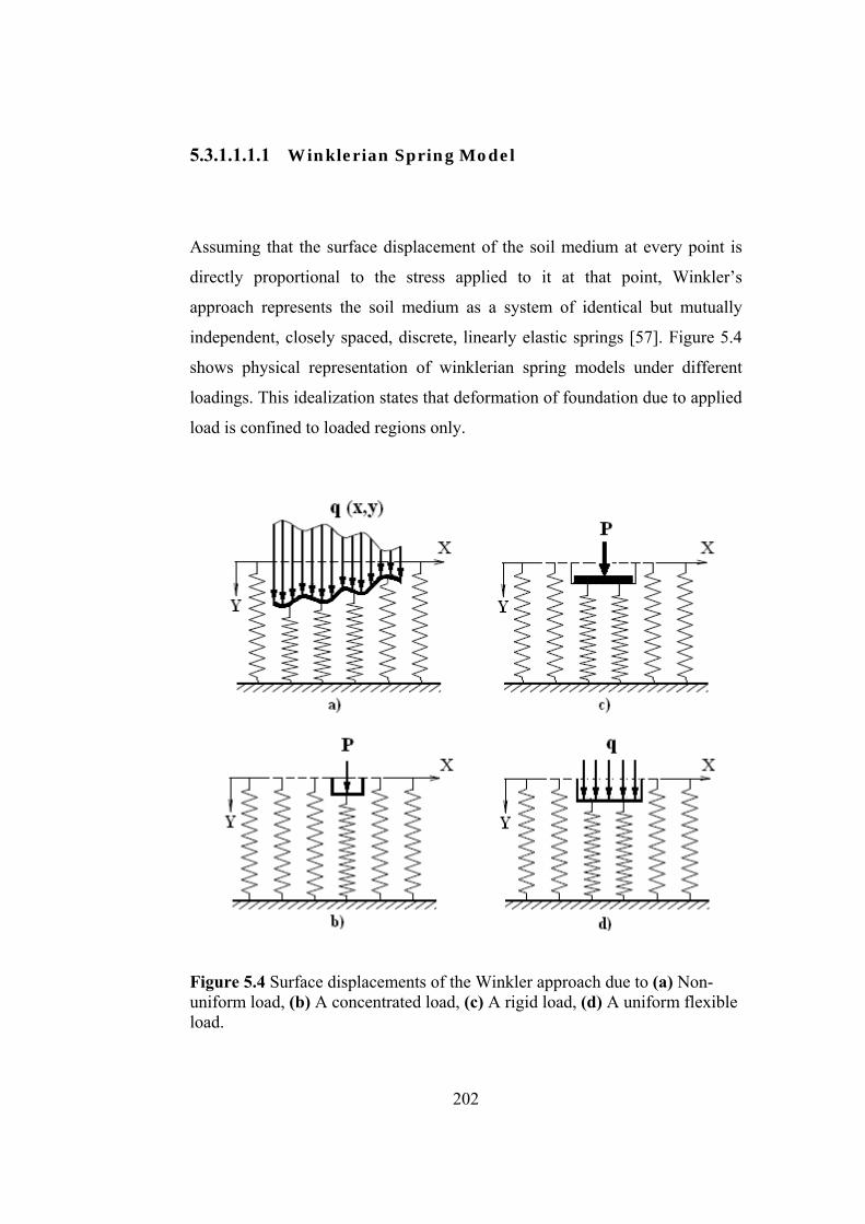
shows physical representation of winklerian spring models under different

loadings. This idealization states that deformation of foundation due to applied

load is confined to loaded regions only.

Figure 5.4 Surface displacements of the Winkler approach due to (a) Non-uniform load, (b) A concentrated load, (c) A rigid load, (d) A uniform flexible load.

203

According to Winkler approach, force-deformation relationship of elastic

springs at any point is given by;

kyP (5.1)

Where;

P is the pressure, k is the coefficient of sub-grade reaction or sub-grade

modulus, and y is the deflection.

There have been a number of soil–structure interaction studies [86–90], based

on the Winkler hypothesis for its simplicity. The main problem with the use of

this model is the determination of the stiffness of elastic springs used to

replace the soil below foundation. Since the Winkler model has only one

parameter, what is called the sub-grade stiffness, to idealize the physical

behavior of the sub-grade, care must be taken to determine it numerically to

use in a practical problem.

Therefore, several methods such as Plate load test, Consolidation test, tri-axial

test, CBR test, proposed in the literature to estimate the modulus of sub-grade

reaction.

Plate load test are generally used to determine bearing capacity and settlement

of shallow footings. This test is conducted by pressing a steel bearing plate

into the surface to be measured with a hydraulic jack. Using dial micrometers

near the plate edge, the resulting surface deflection is read and the modulus of

sub-grade reaction is determined by the following equation

(5.2)

204

Where;

k represents the modulus of sub-grade reaction (spring constant), P and Δ are

applied pressure and measured deflection respectively.

Consolidation can be defined as the decrease in the volume of a soil due to the

expulsion of water. An undisturbed sample of cohesive soil is used in the

laboratory consolidation test to determine its compressibility characteristics.

To obtain these, under different loadings, the change in the height of the soil

sample, resulting from a sequence of vertical stress, is monitored. By plotting

the graphs of the volumetric strain versus applied vertical stress at the end of

each load increment, desired settlement parameters can be achieved.

Tri-axial tests are reliable and widely used methods to determine the

mechanical behavior of soils. In this test, first a cylindrical sample of soil is

prepared and put into a tri-axial testing apparatus. Then, it is laterally confined

by a membrane and radial stress is applied by pressurizing water in a chamber.

Afterwards, axial deformations, volume changes, stress distributions and thus

sub-grade stiffness are determined.

The California bearing ratio (CBR) can be pointed out as a penetration test for

the evaluation of mechanical strength of sub-grades. It was developed by the

California Department of Transportation. The test is conducted by measuring

the pressure necessary for the penetration of a soil sample with a plunger of

standard area. After, this value is divided by the pressure required to obtain an

equal penetration on a standard crushed rock material. Sub-grade stiffness is

then obtained by using this value.

205

5.3.1.1.1.2 Elastic Continuum Models

Elastic continuum model is a conceptual approach of physical representation

of the infinite soil media (Figure 5.5). Soil mass is basically composed of

discrete particles compacted by some inter-granular forces. Boundary

distances and loaded areas, very large compared to the size of the individual

soil grains, are the common features of the problems dealt in soil mechanics.

Therefore, in effect, the body involving discrete molecules gets transformed

into a macroscopic equivalent prone to mathematical analysis. So, it seems to

be very reasonable to invoke to the theory of continuum mechanics for

idealizing the soil media [91].

Figure 5.5 Typical surface displacement profiles of an elastic continuum

subjected to, a) A line load P, b) A uniform load q of width a.

The analysis of elastic continuum model is similar to the one of a semi-

infinite, homogeneous, isotropic, linear elastic solid subjected to a

206

concentrated force acting normal to the plane boundary, where the theory of

elasticity is used. In this case, the behavior of soil medium is represented by

some continuous functions. Hence, this application of continuum theory of

elasticity to soil-foundation interaction presents a complex boundary value

problem. During the analysis, it is assumed that the distribution of

displacements and stresses in soil medium remain continuous under the action

of external force systems.

The simplicity of the input parameters such as modulus of elasticity and

Poisson’s ratio can be pointed out as an important advantage of this approach.

Besides, this approach provides much information on the stress and

deformations within soil mass. However, it is observed that for soil in reality,

the surface displacements away from the loaded region decreased more rapidly

than what is predicted by this approach [57]. Moreover, there exists inaccuracy

in reactions calculated at the outer borders of the foundation. These drawbacks

conclude that this idealization is not only difficult to compute but often fails to

represent the physical behavior of soil very closely, too.

5.3.1.1.1.3 Two Parameter Elastic Models

Two parameter models posses some of the characteristics features of

continuous elastic continuum models. The term "Two Parameter" means that

the model is defined by two independent elastic constant. Various two

parameter models have been developed along following different lines.

a) The first type is originated from the discontinuous Winkler's model and

removes this discontinuity by providing mechanical interaction between

the individual spring elements by use of either elastic membranes and

207

elastic beams or elastic layers capable of purely shearing deformations

[92].

b) The models included in the class of second approach are related to the

elastic continuum model and introduce constraints or simplifying

assumptions with respect to the distribution of displacements and

stresses [92].

5.3.1.1.1.4 Finite Element Models

Because of the fact that the scope of numerical methods is wider than that of

analytical methods, the use of general-purpose finite element method has

gained a great increase to study the complex interactive behavior. The method

is so general that it is possible to model many complex conditions with a high

degree of accuracy, including nonlinear stress–strain behavior, non-

homogeneous material conditions, and changes in geometry and so on.

The method is a special extended form of matrix analysis based on variational

approach, in which the whole system, that is the frame, soil and foundation in

this study, is discretized into a finite number of elements connected at different

nodal points as shown in Figure 5.6. Displacements functions, i.e., the

displacement within the element is unknown and therefore to be assumed in a

sensible manner. Hence, knowing the stiffness matrix for each element, overall

stiffness matrix may be obtained. Then, from the boundary conditions and

global loading conditions nodal unknowns may be generated.

208

Figure 5.6 Representation of soil-structure interaction with finite element

approach

5.3.1.1.2 Elastic-Plastic, Perfectly Plastic Models

Elastic-plastic or irreversible behavior of the soil medium is not considered in

the elastic soil models. The basic difference between the purely elastic and

elastic-plastic models is that, in the latter case, the stresses that can be induced

in the soil medium are restricted owing to the introduction of a yield or failure

criterion. Foundation model, presented in [92], can be pointed out as an

example of a purely mechanical type. This model assumes that the shear layer

used to interconnect the spring elements of the Pasternak foundation model

[92] has the ability of sustaining finite shearing stresses. The shear stress-shear

strain relationship for the elastic layer is of an elastic-rigid plastic type. By use

of this particular model, the distribution of contact stresses beneath a rigid

209

foundation, which is subjected to a symmetric load, is investigated. The results

show that the consideration of such yielding characteristics can change both

the magnitude and distribution of contact stresses that are developed at soil-

foundation interface.

5.3.1.2 Winklerian Modeling of Planar Steel Frame-Soil Interaction System

In some cases, a structural support may not fully prevent motion, which may

result in undesired effects in the response of structural system as a whole. The

designers, thus, want to investigate the response of a structure resting on a soil

mass that deforms with load. Provided that the properties of the soil are

known, it may be possible to represent the supporting material by a set of

springs. Winkler model, known as Winklerian springs, is the most popular

modeling used to solve the soil-structure interaction problems.

Figure 5.7 illustrates the representation of a simple beam, displacements of

which are controlled by one rigid and one semi-rigid support. At joint 1, beam

has two degrees of freedom of rotation and horizontal displacement, which

means that it is restrained only along vertical direction. Thus, only one spring

is required to represent the supporting soil under the beam.

In Figure 5.7a, the original form of a beam member is shown. As stated in

Figure 5.7b, Winkler spring may be used to represent the support. Rigidity of

this physical element is included in the overall stiffness matrix by assuming it

as an additional structural element as shown in Figure 5.7c.

210

Figure 5.7 A simple beam element with one rigid and one semi-rigid supports.

In the case where the supported joints are fully restrained as shown in Figure

5.8, soil is represented by three spring elements, horizontal, vertical and

rotational stiffness of which are symbolized by kx , ky , kθ respectively. In the

matrix formulation these values are added to the main diagonal term of the

degree of freedom in the direction of the spring. Numerical values of these

coefficients are determined from the experimental soil tests described in

previous sections.

Figure 5.8 Representation of a simple planar frame-soil interaction

211

A more realistic representation of soil-structure interaction system can be

achieved by including foundation slab in the analysis (Figure 5.9). In this

study, the steel frame is assumed to be supported by rigid strip foundations

made up of reinforced concrete and soil, on which these foundation slabs rest,

is simulated by elastic springs as described previously.

Figure 5.9 Soil-foundation-structure interaction systems

To do this, a set of closely spaced independent fictitious vertical springs are

inserted underneath the rigid footings along their lengths [93]. Stiffness of

rotational springs is assumed to be zero and only one horizontal spring is used

to support the system along x-direction. Each of these vertical springs,

thereby, of the axial elements which can be used instead, has the same

experimental stress-strain relationship as that of granular soil, which is

obtained by carrying out standard drained tri-axial compression test conducted

212

in [94] (Figure 5.10a). Using this relationship, a load-settlement diagram can

be produced (Figure 5.10b). Through the use of this diagram, the nonlinear

behavior of soil is taken into account in the analysis, by performing an

iterative nonlinear analysis method.

Figure 5.10 a) Stress-strain curves for drained triaxial test on dense silica

sand, b) Linearized load-deformation diagram for

The method conducted, first approximates this nonlinear load-settlement

diagram by a number of straight lines (Figure 5.10b). The intersection points

of these lines indicate that as the load increases the slope of the linear

segments changes implying the variations in the axial stiffness (EA) of the

213

member. In other words, the modulus of elasticity becomes a variable which

describes soil behavior at a particular stress condition. The effect of sign

changes from positive to negative in the slope of load-deformation diagram is

also considered by substituting (-EA) for the axial stiffness of the member.

These stress (σ1-σ7) and corresponding modulus of elasticity (E1-E7) values

are tabulated in Table 5.1. Axial stiffness of horizontal member is taken from

[95] as Sk = 0.04714 kN/cm and the dimensions of foundation slab is

considered as 200x50x70cm.

Table 5.1 Stress-strain and corresponding modulus of elasticity values of each

linear segment obtained from nonlinear stress-stress curve.

Linear segment number

1 2 3 4 5 6 7

σ(kN/cm2) 0.05 0.07 0.082 0.088 0.09 0.089 0.079

ε(%) 0.4 0.7 1.3 2.2 3.4 4.5 9.2

E(kN/cm2) 12.5 6.667 2 0.667 0.167 -0.111 -0.212

Once the axial stiffness of all the members are specified up to failure, the

nonlinear analysis is easily carried out by allowing these changes in the

stiffness of the members during the increase of external loads. This is

performed as follows;

1) Foundation is analyzed under the external loads and member forces and

joint displacements are determined.

214

2) As the load is increased, the initial stiffness of the structure does not

change until one of the axial elements reaches its critical point. This

change is controlled by load factor which is obtained by first computing

the lowest incremental load factor.

∆λi = ( CFi - |Paim| ) / Pi

m i =1,...,nm (5.3)

Where;

i is the incremental load factor, iCF is critical force for member i,

maiP and m

iP represent the actual force and the force due to external loads

in member i at step m. It is clear that initially actual member forces are

equal to zero. If the minimum in the equation (5.3) is m then the next

critical load factor is obtained as;

mmm 1 (5.4)

3) Pa and xa, representing the actual member forces and joint

displacements, are updated in every cycle as;

111 )( mmmma

ma PPP (5.5)

111 )( mmmma

ma xxx (5.6)

215

Where;

m and 1m are the load factors at the current and previous steps

respectively while P and x represent the member forces and joint

displacements obtained by linear analysis in step number m.

4) After the critical point is reached, (EA)j, which is the axial rigidity of

member i, is required to be replaced with (EA)j+1 which is specified by

the next portion of the load-deformation diagram. This requires the

reanalysis of the structure with axial member i having stiffness (EA)j+1

resulting new set of member forces and joint displacements.

5) Steps 2, 3, 4 are repeated until the load factor reaches to a predetermined

value u , or settlements become excessive.

It is apparent from the Figure 5.10 that when the procedure moves from one

critical point to another, stiffness coefficient EA/L of each axial element

changes each time. As a result, at each critical point the contribution matrix of

that element is adjusted and stiffness equations are solved to obtain the new set

of member forces and joint displacements.

In order to clarify the working steps of the algorithm the following simple soil-

structure interaction problem where a strip foundation is supported by a

number of axial elements is considered.

216

Figure 5.11 A simple strip foundation-soil interaction problem.

The strip foundation is assumed to be resting on dense silica sand and it is

subjected to external loading, which is also illustrated in Figure (5.11). The

length of the axial elements and the height of the foundation are assumed to be

0.5m and 0.7m, respectively. Cross-sectional area of each axial element is

assumed to be 20cm2 .The geometry of the foundation is shown in the figure in

detail. Linearized load-deformation diagram given in Figure 5.10 is used for

the representation of nonlinear soil.

The foundation is analyzed twice, employing linear and nonlinear analysis

procedures. The settlements obtained in both cases are shown in Figure 5.12. It

is observed that due to the direction of external moments the maximum

settlement occurs at point 6 in linear elastic analysis. However, when

nonlinear analysis procedure is employed, the location of maximum settlement

changes from point 6 to point 2. This is apparent from the fact that the axial

element under external loading reaches to its critical load value before the

others. The soil under this point becomes weaker, leading to greater

settlement. It is also noticed that the difference between the settlements

obtained with linear and nonlinear analysis is 75%.

217

Figure 5.12 Settlements of strip foundation resting on dense silica sand

5.4 Particle Swarm Optimization Design of Rigid and Semi-Rigid Steel Frames Including Soil-Structure Interaction

In this section, optimum design algorithms for rigid and semi-rigid steel

frames where the soil-structure interaction is included are introduced. The

previous optimum design algorithm is extended the design algorithm to

contain the nonlinear soil analysis in the frame analysis routine. The

procedure can be summarized as follows;

1. The geometry and loadings of the frame including the fictitious

elements that represent the soil are defined. The load-deformation

diagram of nonlinear soil is given. If the beam-to-column connections

are semi-rigid then the connection type is selected. The beams and

columns of the frame are grouped together.

2. Particle swarm design optimization algorithm is started by generating

initial values (positions of particles) for the design variables i.e.

218

sequence numbers of steel profiles in steel section tables for discrete

design. Once the steel sections are specified for the member groups, all

the cross sectional properties such as moment of inertia, sectional

modulus and radius of gyration become available. If the end connections

are partially restrained, connection design process is conducted, i.e. the

connection parameters such as angles, plates, bolts etc. are selected

depending on the connection type decided initially.

3. The frame is analyzed with the steel sections adopted for its members

using analysis subroutine which is based on matrix stiffness method.

Nonlinear analysis of soil elements is also performed. Member end

forces and displacements are computed.

4. Design constraints are then checked by using fly-back mechanism. If the

strength and displacement requirements given in LRFD-AISC [49] are

satisfied then this design is accepted, otherwise, it is discarded and new

one is generated.

5. After feasible designs are obtained, particle swarm iteration process is

initialized. Objective function values, weights of frames belonging to

each design, are calculated. The particle which has the minimum weight

is accepted as the current optimum design. After, values of design

variables are updated using velocity and position update equations of

particle swarm algorithm and new designs are generated.

6. These new design candidates are all analyzed under the external loading

and the design constraints are checked. If all the constraints are

satisfied, weights of these new designs are computed and the lightest

among them is taken as the new optimum design, if it is lighter than the

current optimum.

219

7. This iteration procedure is repeated until the predefined number of

iteration is completed. The design from which has the minimum weight

at the last iteration process is taken as the optimum design.

5.4.1 Design Examples

Two unbraced steel frames are designed using the optimum design algorithm

presented. Frames are assumed to be resting on nonlinear soil. The nonlinear

behavior of the soil is represented by using fictitious axial elements. Distance

between each vertical axial element is assumed to be 50 cm. Differential

settlement of the frames is restricted to 5cm. Besides, when the analysis

procedure is performed, beam-to-column connections are assumed as fully

restrained or partially restrained. Latter approach is implemented in such a

way that the end connections are designed with end plate without column

stiffener model. Overall weights of fully supported and partially supported

versions of each frame are compared to have an idea about how much the

consideration of soil affects the behavior of complete structure. In the design

process the discrete set from which the design algorithm selects the sectional

designations for frame members is considered to be the complete set of 272

W-sections starting from W100x19.3 to W1100x499mm as given in LRFD-

AISC [49].

5.4.1.1 Three Storey-Two Bay Steel Frame

The two bay, three storey frame shown in Figure 5.13 is selected as first

design example, to demonstrate the application of the optimum design

220

algorithm developed. The dimensions, member grouping and the external

loading of the system are also shown in the figure. The upper bound imposed

on lateral deflections of the top storey joints is limited to 1/300 of the frame

height, which corresponds to 30.48 mm. The frame members are collected in

two different groups. Columns are considered to be group 1 while beams are

taken as group 2 as shown in the figure. Hence there are only two design

variables in the design problem. A single distributed load of 40kN/m is applied

on each beam of the frame and lateral load of 20kN is applied to each storey

level. The strength capacities of steel members are computed according to

LRFD-AISC [49]. Beam-to-column connections are designed as end plate

without column stiffeners model. Each foundation slab has five vertical axial

elements and one horizontal axial element to support the structure along

horizontal direction as shown in Figure 5.13.

Figure 5.13 Three storey-two bay steel frame

221

The frame is designed twice considering both semi-rigid and rigid beam-to-

column connections. The design history of these runs is shown in Figure 5.14.

Best designs are tabulated in Table 5.2 with section designations attained for

each member group. As indicated in this table, when the nonlinear behavior of

soil is neglected, particle swarm method based optimum design algorithm

produces a rigidly connected frame which has the minimum weight of which

is 12005.990kg. On the other hand, the one obtained under the consideration

of nonlinear soil has the weight of 12459.16kg. This means that the inclusion

of soil-structure interaction in the design algorithm leads to an increase in the

overall weight of the frame. In the former and latter design, the governing

design constraint is the maximum strength ratio, with the same value of 0.98.

On the other hand, partially restrained frames, designed by use of design

algorithms where the soil-structure interaction is excluded and included, have

the weights of 12358.45kg and 13192.05kg respectively. Dominant constraint

of both designs is the maximum strength ratio with the values of 0.93 and

1.00, respectively. It is clear from the results that when the nonlinear behavior

of soil is taken into account, the algorithm produces 4% heavier frame in the

case of rigid connections and 7% heavier frame in the case of semi-rigid

connections.

222

Table 5.2 Optimum designs for three-storey, two-bay steel frame.

11000

12000

13000

14000

15000

16000

17000

18000

19000

0 500 1000 1500 2000 2500 3000 3500 4000 4500 5000

Number of iterations

Bes

t fe

asib

le d

esig

n (

kg )

Rigid connect., fixed support

Rigid connect., soil-structure interact.

Semi-rigid connect., fixed support

Semi-rigid connect., soil-structure interact.

Figure 5.14 Design history graph for three-storey, two-bay steel frame.

Group No.

Member Type

Fixed support Soil-structure interaction

Fully rigid connect.

Wsections-Area(cm2)

Semi-rigid connect.

(End plate) Wsections-Area(cm2)

Fully rigid connect.

Wsections-Area(cm2)

Semi-rigid connect.

(End plate) Wsections-Area(cm2)

1 Column W250X73 (92.8) W250X115 (146) W760X134(170) W310X454(578) 2 Beam W690X152 (194) W610X140 (179) W760X134(170) W690X192(244)

Max. Int. St. Drift Ratio

0. 30 0.42 0.93 0.60

Max. Strength Ratio 0.98 0.93 0.98 1.00 Top storey drift (cm) 0.80 1.100 2.329 1.521 Minimum Weight.

kg(kN) 12005.990 (117.738)

12358.45 (121.194)

12459.16 (122.182)

13192.05 (129.369)

223

5.4.1.2 Four Storey-Four Bay Steel Frame

Four storey-four bay steel frame is considered as the second example.

Loadings and dimensions of the frame are shown in Figure 5.15. The frame

consists of thirty-six members that are collected in two groups as shown in the

figure. Columns are taken as group 1 and beams are considered as group 2.

The lateral displacement of the top storey is limited to 4cm and maximum

inter-storey drift is restricted to 1cm. The modulus of elasticity is 200kN/mm2.

A single distributed load of 35 kN/m and a single lateral load is applied to

each horizontal member of the frame.

Figure 5.15 Four storey-four bay steel frame

224

The optimum W-section designations of semi-rigid and rigid frames obtained

by the particle swarm method are given in Table 5.3. The design of semi-rigid

frame resting on nonlinear soil is attained after 760 iterations and the

minimum weight is 7290.995kg while the one, produced under the

consideration of supports as fully rigid, has the minimum weight of

6167.268kg which is obtained after 160 iterations. In the case of rigid beam-

column connection resting on rigid supports, the minimum weights are

obtained as 7219.616kg and 5914.37kg respectively. It is noticed that the

maximum strength ratio governs the designs. Design history graphs of this

frame are shown in Figure 5.16. It is noticed that the rigid frame produced by

the algorithm which includes the soil-structure-interaction is 22% heavier than

the one having fixed supports. Similarly, the same approach leads to the

production of 18% heavier frame in the case of semi-rigid beam-to-column

connections.

Table 5.3 Optimum designs for four-storey, four-bay steel frame.

Group No.

Member Type

Fixed support Soil-structure interaction

Fully rigid connect.

Wsections-Area(cm2)

Semi-rigid connect.

(End plate) Wsections-Area(cm2)

Fully rigid connect.

Wsections-Area(cm2)

Semi-rigid connect.

(End plate) Wsections-Area(cm2)

1 Column W150X37.1 (47.3) W360X44 (57.3) W360X51(64.5) W410X60 (75.8) 2 Beam W410X46.1 (58.9) W360X44 (57.3) W460X52(66.3) W410X46.1 (58.9)

Max. Int. St. Drift Ratio

0. 47 0.57 0.58 0.50

Max. Strength Ratio 0.99 0.95 0.92 0.95 Top storey drift (cm) 1.59 1.96 1.92 1.699 Minimum Weight.

kg(kN) 5914.37 (58.00)

6167.268 (60.480)

7219.616 (70.80)

7290.995 (71.50)

225

5000

6000

7000

8000

9000

10000

11000

0 500 1000 1500 2000 2500 3000

Number of iterations

Bes

t fe

asib

le d

esig

n (

kg )

Rigid connect., fixed support

Rigid connect., soil-structure interact.

Semi-rigid connect., fixed support

Semi-rigid connect., soil-structure interact.

Figure 5.16 Design history graph for four-storey, four-bay steel frame.

226

CHAPTER 6

SUMMARY AND CONCLUSIONS

6.1 Overview and summary of the thesis

In this study, new approaches are developed for the optimum design of rigid

and semi-rigid unbraced plane steel frames including soil-structure interaction.

This study can be divided into four parts, the results obtained in each of which

are discussed in the following.

In the first part of the study particle swarm optimization (PSO) algorithm is

introduced. It is intended in this section to investigate the performance of this

technique in the solution of benchmark problems. First benchmark problem

solved with this algorithm is called the Himmelblau’s function [62] which has

five design variables and three constraints. PSO result of this problem is -

30665.40, which is the second best objective function value among the ones

obtained with four different optimization methods. Second example is the

welded beam design in which the PSO algorithm shows great performance.

The minimum objective function value obtained with PSO algorithm is 25%

lighter than the best of the rest. Similarly, in the pressure vessel design and

spring design problems, PSO obtained the best results. During these tests, PSO

parameters are also analyzed so that the most appropriate ones are determined.

These observations indicate that the variations in the parameter set have great

effect on the performance of the algorithm. It is noticed that even only change

227

of one parameter in the set can lead to a huge disorder in the convergence and

thereby the final result of the problem. This fact comes from the stochastic

nature of combinatorial optimization algorithms. On the other hand, it is also

noticed that the PSO algorithm has a better convergence rate in the solution of

benchmark problems. It does not require much computation time. Besides, the

results obtained at the end of the iteration process do imply that the technique

is robust and can be applied to the structural design problems. One of the

previous studies, carried out by He et al. [22] has stated the same conclusion.

In the second part of the study, the minimum weight design of seven unbraced

steel frames is presented. Each numerical example is solved with both

continuous and discrete design algorithms. It is observed that the assumption

of continuous set of sections produces 9.5%, 9.6%, 10%, 24%, 34%, 16%,

57% lighter frames. These values imply that the relative difference between

the weights of best designs obtained with each approach is problem dependent.

Additionally, the ascending trend in the values with increasing number of

stories, with the exception of the ten-story-three-bay frame, demonstrate the

advantages of continuous over discrete design with increasing number of

stories. Therefore, approaching the design from discrete to continuous through

the use of built-up sections for a selected number of members might prove to

be economically advantageous in the case of high-rise building frames.

The third part of the study is dedicated to the optimum design of unbraced

steel frames with partially restrained connections. Two types of end

connections are considered in this section. Namely, end plate without column

stiffeners and top and seat angle with web cleats (TSWC). First six examples

are designed with both connection types separately and only the former

connection type is used for the rest. The results indicate that the consideration

of connection flexibility in the design leads to an increase in the overall

weight. Additionally, it is observed that the design algorithm finds much

228

heavier frames when the connections are modeled as TSWC. For example, if

the three storey-three bay steel frame is taken into consideration, it can be

clearly seen that the optimum frame with TSWC is 2.3% heavier than the one

with end plates without column stiffeners. This is due to the high amount of

dependent connection parameters in the design and the insufficient variety of

angle sections given in the ready angle list.

In the last part, the effect of soil-structure interaction is considered in the

optimum design of steel frames. Both types of end connections are taken into

account in the design. As expected, the inclusion of soil-structure interaction

in the design leads to a considerable increase in the overall weight. It is

apparent from the results that this is valid for all examples. For example, in the

problem of four-storey, four bay steel frame, the algorithm produces 22%

heavier rigid frame and 18% heavier semi-rigid frame, when the soil

nonlinearity is included. It is also clear from the results that as the number of

story increases, the effect of soil nonlinearity on the overall weight also

increases.

6.2 Conclusions

In this study, the particle swarm optimizer is used to develop an optimum

design algorithm for moment resisting steel frames. Additionally, the

flexibility of beam-to-column connections is also taken into account in the

structural analysis of the frame. End connection models of top and seat angle

with web cleats and end plate without column stiffeners are used to represent

the beam-to-column connections. Due to the fact that the connection flexibility

affects the distribution of forces in the frame and leads to an increase in the

drift of whole structure, P-∆ effect is required to be considered in the frame

229

analysis. Further, the soil-structure interaction is included in the design

algorithm. Contrary to the practical implementations in which the columns are

connected to the soil with fixed support, the frames in the present study are

modeled as it is supported with the foundations resting on nonlinear elastic

soil. This is achieved through the use of Winkler springs. The nonlinear

behavior of soil is taken into account in the analysis, by performing an

iterative nonlinear analysis method.

The particle swarm optimization based design algorithm is mathematically

quite simple but effective in finding the solutions of combinatorial

optimization problems. The optimum design algorithm presented selects

optimum W-sections from American steel sections table for beams and

columns of unbraced rigid and semi-rigid steel frames such that design

constraints described in LRFD-AISC are satisfied and the frame has the

minimum weight. Continuous numbers generated in the algorithm are

converted to integer ones with rounding off method and these discrete

variables are used to obtain sequence numbers of ready steel section list.

Constraints are handled with fly-back mechanism and feasible ones being

candidate solutions to give the minimum frame weight are determined.

Numerical examples show that rounding-off and fly-back mechanisms are

effective in particle swarm optimization technique.

In view of the results obtained, it can be concluded that the inclusion of joint

flexibility and soil-structure interaction in the analysis leads to a change in the

response of the structural members and therefore an increase in the overall

weight of the frame. It is noticed that when the partially restrained behavior of

connections is considered, the algorithm produces heavier frames. Besides, the

effect of soil-structure interaction results in a further increase in the overall

weight. Therefore, to achieve a more realistic design one should perform the

structural analysis through the consideration of these behaviors.

230

REFERENCES

[1] W.F. Chen, “Practical Analysis for Semi-rigid Frame Design”, World Scientific, Singapore (1999) 268-275.

[2] E.S. Kameshki, M.P. Saka, “Optimum design of nonlinear steel frames

with semi-rigid connections using a genetic algorithm”, Computers and Structures 79 (2001) 1593-1604.

[3] M. Dorigo, G.D. Caro, L.M. Gambardella, “An algorithm for discrete

optimization”, Artificial Life 5 (1999) 137-172.

[4] R.H. Gallagher, O.C. Zienkiewicz, “Optimum Structural Design; Theory and Applications”, John Wiley and Sons, NY, USA (1973) 150-175.

[5] J.S. Arora, “Optimization of Structural and Mechanical Systems”, World Scientific, Singapore (2007) 59-195.

[6] P.W. Christensen, “An Introduction to Structural Optimization”, Springer, Linköping, Sweden (2008) 179-200.

[7] H.A. Eschenauer, C. Mattheck , N. Ohloff, “Engineering optimization

in design processes”, Proceedings of the International Conference, Karlsruhe Research Center, Karlsruhe, Germany (1990).

[8] R.T. Haftka, “Elements of Structural Optimization”, Springer,

Dordrecht, Netherlands (1992) 347-387.

[9] M. Kurt, “Stochastic Optimization Methods”, Springer, Munich, Germany (2005) 3-43.

[10] J. Holland, “Genetic algorithms and the optimal allocation of trials”,

Society for Industrial and Applied Mathematics Journal of Computing 2 (1973) 88-105.

[11] F. Glover, “Tabu Search”, Kluwer Academic Publications, MA, USA (1997) 1-54.

231

[12] Y.L. Kwang, M.A. El-Sharkawi, “Modern Heuristic Optimization Techniques: Theory and Applications to Power Systems”, Institute of Electrical and Electronics Engineers Press, NJ, USA (2008) 43-147.

[13] B.V. Babu, G.C. Onwubolu, “New Optimization Techniques in Engineering”, Springer, Berlin, Germany (2008) 101-123.

[14] Z.W. Geem, J.H. Kim, “A new heuristic optimization algorithm: Harmony search”, Simulation 76 (2001) 60-68.

[15] Z.W. Geem, K.S. Lee, Y. Park, “Application of harmony search to vehicle routing”, American Journal of Applied Sciences 12 (2005) 1552-1557.

[16] O.K. Erol, I. Eksin, “A new optimization method: Big bang-big crunch”, Advances in Engineering Software 37 (2006) 106-111.

[17] J. Kennedy, R. Eberhart, “Particle swarm optimization”, Institute of Electrical and Electronics Engineers Press 4 (1995) 1942-1948.

[18] J. Kennedy, R.C. Eberhart, “A discrete binary version of the particle

swarm algorithm”, Proceedings of the World Multi-Conference on Systemic, Cybernetics and Informatics, NJ, USA (1997).

[19] K.E. Parsopoulos, M.N. Vrahatis, “Particle swarm optimization method

for constrained optimization problems”, Intelligent Technologies Theory and Applications: New Trends in Intelligent Technologies 76 (2002) 214-220.

[20] P. Fourie, A. Groenwold, “The particle swarm optimization algorithm

in size and shape optimization”, Structural and Multidisciplinary Optimization 23 (2002) 259-267.

[21] S. He, Q.H. Wu, J.Y. Wen, J.R. Saunders, R.C. Paton, “A particle

swarm optimizer with passive congregation” Biosystem 78 (2004) 135-147.

[22] S. He, E. Prempain, Q.H. Wu, “An improved particle swarm optimizer

for mechanical design optimization problems”, Engineering Optimization 36 (2004) 585-605.

232

[23] M.F. Tasgetiren, Y.C. Liang, M. Sevkli, G. Gencyilmaz, “Particle swarm optimization algorithm for makespan and maximum lateness minimization in permutation flowshop sequencing problem”, Proceedings of the Fourth International Symposium on Intelligent Manufacturing Systems, Sakarya, Turkey (2004).

[24] H. Liu, S. Shichang, A. Ajith, “Particle swarm approach to scheduling

work-flow applications in distributed data-intensive computing environments”, Proceedings of the Sixth International Conference on Intelligent Systems Design and Applications, Jinan, China (2006).

[25] M.S. Arumugam, M.V.C. Rao, A. Chandramohan, “A new and

improved version of particle swarm optimization algorithm with global–local best parameters”, Knowledge and Information Systems 16 (2008) 331-357.

[26] L. Li, Z. Huang, F. Liu, “An improved particle swarm optimizer for

truss structure optimization”, Lecture Notes in Computer Science, Springer 4456 (2007) 1-10.

[27] A. Kaveh, S. Talatahari, “A hybrid particle swarm and ant colony

optimization for design of truss structures”, Asian Journal of Civil Engineering 9 (2008) 329-348.

[28] A. Carlos, C. Coello, “Theoretical and numerical constraint handling

techniques used with evolutionary algorithms: A survey of the state of the art”, Computer Methods in Applied Mechanics and Engineering 191 (2002) 1245–1287.

[29] M.R. Khan, “Optimality criterion techniques applied to frames having

general cross-sectional relationships”, American Institute of Aeronautics and Astronautics Journal 22 (1984) 669-676.

[30] “Manual of Steel Construction: Allowable Stress Design”, American

Institute of Steel Construction, CA, USA (1989) 85-256. [31] C.V. Camp, S. Pezeshk, G. Cao, “Design of framed structures using a

genetic algorithm”, Proceedings of Advances in Structural Optimization, NY, USA (1997).

[32] M.W. Huang, J.S. Arora, “Optimal design steel structures using

standard sections”, Structural Optimization 14 (1997) 24-35.

233

[33] M.P. Saka, E.S. Kameshki, “Optimum design of unbraced rigid frames”, Computers and Structures 69 (1998) 433-442.

[34] M.P. Saka, E.S. Kameshki, “Optimum design of multistory sway steel

frames to BS 5950 using a genetic algorithm”, Journal of Constructional Steel Research 65 (2009) 36-43.

[35] H.S. Park, C.W. Sung, “Optimization of steel structures using

distributed simulated annealing algorithm on a cluster of personal computers”, Computers and Structures 80 (2002) 1305-1316.

[36] C.V. Camp, J.B. Barron, P.S. Scott, “Design of steel frames using ant

colony optimization”, Journal of Structural Engineering 131 (2005) 369-379.

[37] S.O. Degertekin, “A comparison of simulated annealing and genetic

algorithm for optimum design of non-linear steel space frames”, Structural and Multidisciplinary Optimization 34 (2007) 347-359.

[38] M.P. Saka, “Optimum design of steel frames using stochastic search

techniques based on natural phenomena”, Saxe-Coburgh Publications, Stirlingshire, UK 6 (2007) 105-147.

[39] E. Dogan, M.P. Saka, "Optimum design of unbraced steel frames to the

LRFD-AISC code using particle swarm optimization", Proceedings of the Ninth International Conference on Computational Structures Technology, Athens, Greece (2008).

[40] W.F. Chen, N. Kishi, "Semi-rigid steel beam-to-column connections:

data base and modeling", Journal of Structural Engineering 115 (1989) 105-119.

[41] S.H. Hsieh, G.G. Deierlein, “Nonlinear analysis of three-dimensional

steel frames with semi-rigid connection”, Computers and Structures 41 (1990) 995-1009.

[42] L. Xu, “Practical Computer-based Analysis of Semi-rigid Steel

Frames”, Practical Analysis for Semi-Rigid Frame Design (2000) 176-199.

[43] M.A. Hadianfard, R. Razani, "Effects of semi-rigid behaviour of

connections in the reliability of steel frames", Structural Safety 25 (2003) 123-138.

234

[44] L. Xu, A.N. Sherbourne, D.E. Grierson, “Optimal cost design of semi-rigid, low-rise industrial frames”, Engineering Journal 32 (1995) 87-97.

[45] L. Xu, “Design and optimization of semi-rigid framed structures”,

Recent Advances in Optimal Structural Design 147 (2002) 134-150. [46] M.S. Hayalioglu, S.O. Degertekin, “Minimum cost design of steel

frames with semi-rigid connections and column bases via genetic optimization”, Computers and Structures 83 (2005) 1849-1863.

[47] E.S. Kameshki, M.P. Saka, “Genetic algorithm based optimum design

of nonlinear planar steel frames with various semi-rigid connections”, Journal of Constructional Steel Research 59 (2003) 109-134.

[48] E. Doğan, M.P. Saka, “Particle swarm optimization design of moment

resisting steel frames with semi-rigid connections to LRFD-AISC”, Proceedings of the Eight World congress on Structural and Multidisciplinary Optimization (2009).

[49] LRFD-AISC, “Load and Resistance Factor Design”, American Institute

of Steel Construction, IL, USA (1999) 62-564. [50] D. Morris, “Interaction of continuous frames and soil media”, Journal

of Structural Engineering 5 (1966) 13-43. [51] I.K. Lee, P.T. Brown, “Structures–foundation interaction analysis”,

Journal of Structural Engineering 11 (1972) 2413-2431. [52] K.S. Subbaa, H. Rao, B.V. Sharaadaa, “Interaction analysis of frames

with beam footing”, Indian Geotechnical Conference Roorkee l (1985) 389-395.

[53] J. Lysmer, R.L. Kuhlemeyer, “Finite dynamic model for infinite

media”, Journal of Engineering Mechanics 95 (1969) 859–877. [54] P.N. Godbole, M.N. Viladkar, J. Noorzaei, “Nonlinear soil-structure

interaction analysis using coupled finite-infinite elements”, Computers and Structures 36 (1990) 1089-1096.

[55] D.C. Rizos, “Development of a BEM-FEM coupled algorithm for

dynamic soil-structure interaction analysis”, Proceedings of the United States Association for Computational Mechanics Congress, CO, USA (1999).

235

[56] J.H. Park, J. Park, K. Park, S. Ok, “Analysis of soil-structure interaction considering complicated soil profile”, Proceedings of the International Conference on Numerical Methods and Applications, Borovets, Bulgaria (2007).

[57] S.C. Dutta, R. Roy, “A critical review on idealization and modeling for

interaction among soil–foundation–structure system”, Computers and Structures 80 (2002) 1579-1594.

[58] A.B. Vesic, “Beams on elastic subgrade and Winkler’s hypothesis”,

Proceedings of the International Conference on Soil Mechanics and Foundation Engineering, Paris, France (1961).

[59] M.M. Allam, K.S. Subba Rao, ”Frame soil interaction and Winkler

model”, Institution of Civil Engineers Journal 2 (1991) 477-494. [60] S. Hackwood, J. Wang, “The engineering of cellular robotic systems”,

Proceedings of Institute of Electrical and Electronics Engineers Internatioal Symposium, Arlington, Virginia, USA (1988).

[61] M.M. Millonas, "Swarms, phase transitions, and collective

intelligence", Artificial Life 3 (1994) 417-445. [62] D.M. Himmelblau, “Applied Nonlinear Programming”, Mc-Graw Hill,

Daryaganj, New Delhi, India (1972) 35-152. [63] M. Gen, R. Cheng, “Genetic Algorithms and Engineering Design”,

John Wiley and Sons, NY, USA (1997) 42-96.

[64] T.P. Runarsson, X. Yao, “Stochastic ranking for constrained evolutionary optimization”, Institute of Electrical and Electronics Engineers International Transactions on Evolutionary Computation 4 (2000) 284-294.

[65] K.M. Ragsdell, D.T. Phillips, “Optimal design of a class of welded

structures using geometric programming”, American Society of Mechanical Engineering Journal of Engineering for Industries 98 (1976) 1021-1025.

[66] K. Deb, “Optimal design of a welded beam via genetic algorithms”, American Institute of Aeronautics and Astronautics Journal 29 (1991) 2013-2015.

236

[67] T. Ray, K.M. Liew, “Society and civilization: An optimization algorithm based on the simulation of social behavior”, Institute of Electrical and Electronics Engineers International Transactions on Evolutionary Computation 7 (2003) 386-396.

[68] E. Sandgren, “Nonlinear integer and discrete programming in

mechanical design optimization”, Journal of Mechanical Design 112 (1990) 223-229.

[69] K. Deb, “Geneas: A robust optimal design technique for mechanical

component design”, Evolutionary Algorithms in Engineering Applications 185 (1997) 497-514.

[70] Y.J. Cao, Q.H. Wu, “A mixed variable evolutionary programming for

optimization of mechanical design”, International Journal of Engineering Intelligent Systems for Electrical Engineering and Communications 7 (1999) 77-82.

[71] A.D. Belegundu, “A study of mathematical programming methods for

structural optimization”, International Journal for Numerical Methods in Engineering 21 (1985) 1583-1599.

[72] J.S. Arora, “Introduction to Optimum Design”, McGraw-Hill, NY,

USA (1989) 105-165. [73] C. Coello, A. Carlos, “Use of a self-adaptive penalty approach for

engineering optimization problems”, Computers in Industry 41 (2000) 113-127.

[74] W.M. Jenkins, “Plane frame optimum design environment based on

genetic algorithm”, Journal of Structural Engineering 118 (1992) 3103-3112.

[75] L. Shi, H. Fu, “A delimitative and combinatorial algorithm for discrete

optimum design with different discrete sets”, Computational and Information Science 3314 (2004) 443-448.

[76] D. Schodek, “Structures”, Prentice Hall, NJ, USA (2008) 152-365. [77] A. Kassimali, “Structural Analysis”, Thomson, Ontario, Canada (2005)

89-160.

237

[78] W. McGuire, “Steel Structures”, Prentice Hall, NJ, USA (1968) 236-283.

[79] E. Dogan, M.P. Saka, “Optimum design of steel frames to LRFD-

AISC using particle swarm optimization”, Advances in Engineering Software (under review).

[80] W.F. Chen, “LRFD Steel Design Using Advanced Analysis”, Chemical

Rubber Company Press, NJ, USA (1997) 122-146. [81] M.A. Bhatti, J.D. Hingtgen, “Effects of connection stiffness and

plasticity on the service load behaviour of unbraced steel frames”, Engineering Journal 32 (1995) 21-33.

[82] F.H. Wu, “Semi-Rigid Connections in Steel Frames”, Dissertation

Abstracts International 50 (1989) 228. [83] W.F. Chen, E.M. Lui, “Stability Design of Steel Frames“, Chemical

Rubber Company Press, FL, USA (1997) 205-350. [84] K.I. Majid, “Nonlinear Structures“, London Butterworth, London,

England (1972) 100-115. [85] R. Roy, S.C. Dutta, D. Moitra, “Soil-structure interaction in buildings

with isolated and grid foundations: A critical study on the state of the art with recommendations", The Bridge and Structural Engineers 31 (2002) 15-36.

[86] M. Hetenyi, “Beams on Elastic Foundations”, University of Michigan

Press, MI, USA (1946) 179-214. [87] E.P. Popov, “Successive approximation for beams on elastic

foundations”, Transactions American Society of Civil Engineers 116 (1951) 1083-1108.

[88] A.B. Vesic, “Bending on beams resting on isotropic elastic solid”,

Journal of Engineering Mechanics 2 (1961) 35-53. [89] F. Kramrisch, P. Rogers, “Simplified design of combined footings”,

Journal of Soil Mechanics 87 (1961) 19-44. [90] C.B. Brown, J.M. Laurent, J.R. Tilton, “Beam-plate system on Winkler

foundation”, Journal of Engineering Mechanics 103 (1977) 589-600.

238

[91] ME. Harr, “Foundation of Theoretical Soil Mechanics”, McGraw-Hill, London, England (1966) 150-215.

[92] Y.H. Wang, L.G. Tham, Y.K. Cheung, “Beams and plates on elastic

foundations”, Structural Engineering Materials 7 (2005) 174-182. [93] M.P. Saka, A.R. Buzdar, “Nonlinear analysis of strip foundations

through microcomputers”, Proceedings of the International Conference on Foundation and Tunnels, Edinburgh, England (1989).

[94] J.M. Duncan, C.Y. Chang, “Nonlinear analysis of stress and strain in

soils”, Journal of Soil Mechanics and Foundations 96 (1970) 1629-1653.

[95] J.A. Langer, E.T. Mosley, C.D. Thompson, “Laterally Loaded Deep

Foundations”, American Society for Testing and Materials, PA, USA (1983) 1-30.

239

CURRICULUM VITAE

PERSONAL INFORMATION

Surname, Name : Doğan, Erkan Nationality : Turkish (TC) Date of Place and Birth : 18.03.1981, Erzurum Marital Status : Single Email : [email protected]

EDUCATION

Degree Institution Year of Graduation

BS Atatürk University Civil Eng. 2002

WORK EXPERIENCE

Year Place Enrollment

2004-Present METU Engineering Sciences Dept. Research Assistant

PUBLICATIONS

1) E. Doğan, M.P. Saka, “Optimum design of steel frames to LRFD- AISC using particle swarm optimization”, Computers and Structures (under review).

2) E. Doğan, O. Hasançebi, M.P. Saka, “A refinement of discrete particle

swarm optimization for large-scale truss structures”, Asian Journal of Civil Engineering 10(3) (2009).

INTERNATIONAL CONFERENCE PROCEEDINGS

1) E. Doğan, M.P. Saka, "Particle swarm optimization design of moment resisting steel frames with semi-rigid connections to LRFD- AISC ", Proceedings of Eighth World Congress on Structural and Multidisciplinary Optimization (2009).

240

2) E. Doğan, M.P. Saka, “Optimum design of steel frames to LRFD- AISC using particle swarm optimization”, Proceedings of The Ninth International Conference on Computational Structures Technology (2008).

3) E. Doğan, F. Erdal, M.P. Saka, “Optimum design of grillage systems

under code provisions using particle swarm optimization”, Proceedings of Genetic and Evolutionary Computation Conference (2010).

NATIONAL CONFERENCE PROCEEDINGS

1) E. Doğan, M.P. Saka, "Çelik çerçevelerin LRFD-AISC şartnamesine göre parçacık küme optimizasyon yöntemi kullanılarak optimum boyutlandırılması", XVI. Ulusal Mekanik Kongresi Türkiye (2010).

INTERNATIONAL COURSES AND SEMINARS ATTENDED

1) "High performance computations for engineering" course, 17- 22 May 2009 Pecs Hungary.

2) L.E. Garcia, “Rc structures under extreme loading”, 19-20 February,

2009, Ankara, Turkey.

RESEARCH PROJECTS UNDERTAKEN 1) O.Hasançebi, M. P. Saka, Ö. Kurç, S. Çarbaş, E. Doğan, F. Erdal and

T. Bahçelioğlu, “Optimum Design of Three Dimensional Steel Skeleton Structures Using Stochastic Search Techniques and its National Structural Engineering Applications”, Turkish Scientific and Technical Research Council (TUBITAK), Ankara, Turkey, Project No:108M070, (75000 US$), started on 1st June 2008, To be Completed on:1st December 2010.

2) Middle East Technical University Research 1465 Funding (BAP-2008-03- 03-02).


Recommended