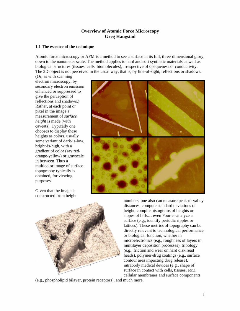
Overview of Atomic Force Microscopy Greg Haugstad

1.1 The essence of the technique Atomic force microscopy or AFM is a method to see a surface in its full, three-dimensional glory, down to the nanometer scale. The method applies to hard and soft synthetic materials as well as biological structures (tissues, cells, biomolecules), irrespective of opaqueness or conductivity. The 3D object is not perceived in the usual way, that is, by line-of-sight, reflections or shadows. (Or, as with scanning electron microscopy, by secondary electron emission enhanced or suppressed to give the perception of reflections and shadows.) Rather, at each point or pixel in the image a measurement of surface height is made (with caveats). Typically one chooses to display these heights as colors, usually some variant of dark-is-low, bright-is-high, with a gradient of color (say red-orange-yellow) or grayscale in between. Thus a multicolor image of surface topography typically is obtained, for viewing purposes. Given that the image is constructed from height

numbers, one also can measure peak-to-valley distances, compute standard deviations of height, compile histograms of heights or slopes of hills… even Fourier-analyze a surface (e.g., identify periodic ripples or lattices). These metrics of topography can be directly relevant to technological performance or biological function, whether in microelectronics (e.g., roughness of layers in multilayer deposition processes), tribology (e.g., friction and wear on hard disk read heads), polymer-drug coatings (e.g., surface contour area impacting drug release), intrabody medical devices (e.g., shape of surface in contact with cells, tissues, etc.), cellular membranes and surface components

(e.g., phospholipid bilayer, protein receptors), and much more.

1

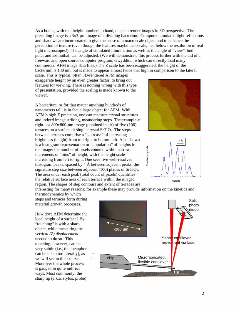
As a bonus, with real height numbers in hand, one can render images in 3D perspective. The preceding image is a 3x3-µm image of a dividing bacterium. Computer simulated light reflections and shadows are incorporated to give the sense of a macroscale object and to enhance the perception of texture (even though the features maybe nanoscale, i.e., below the resolution of real light microscopes!). The angle of simulated illumination as well as the angle of “view”, both polar and azimuthal, can be adjusted. (We will demonstrate this process further with the aid of a freeware and open source computer program, Gwyddion, which can directly load many commercial AFM image data files.) The Z scale has been exaggerated: the height of the bacterium is 180 nm, but is made to appear almost twice that high in comparison to the lateral scale. This is typical; often 3D-rendered AFM images exaggerate height by an even greater factor, to bring out features for viewing. There is nothing wrong with this type of presentation, provided the scaling is made known to the viewer. A bacterium, or for that matter anything hundreds of nanometers tall, is in fact a large object for AFM! With AFM’s high Z precision, one can measure crystal structures and indeed image striking, meandering steps. The example at right is a 800x800-nm image (obtained in air) of five (100) terraces on a surface of single crystal SrTiO3. The steps between terraces comprise a “staircase” of increasing brightness (height) from top right to bottom left. Also shown is a histogram representation or “population” of heights in the image: the number of pixels counted within narrow increments or “bins” of height, with the height scale increasing from left to right. One sees five well-resolved histogram peaks, spaced by 4 Å between adjacent peaks, the signature step size between adjacent (100) planes of SrTiO3. The area under each peak (total count of pixels) quantifies the relative surface area of each terrace within the imaged region. The shapes of step contours and extent of terraces are interesting for many reasons; for example these may provide information on the kinetics and thermodynamics by which steps and terraces form during material growth processes. How does AFM determine the local height of a surface? By “touching” it with a sharp object, while measuring the vertical (Z) displacement needed to do so. This touching, however, can be very subtle (i.e., the metaphor can be taken too literally), as we will see in this course. Moreover the whole process is gauged in quite indirect ways. Most commonly, the sharp tip (a.k.a. stylus, probe)

Height

Num

ber o

f pix

els

4 Å

Split photodiode

~100 µm

chip

Sense cantilever movement via laser

Microfabricated, flexible cantilever

Tip

2

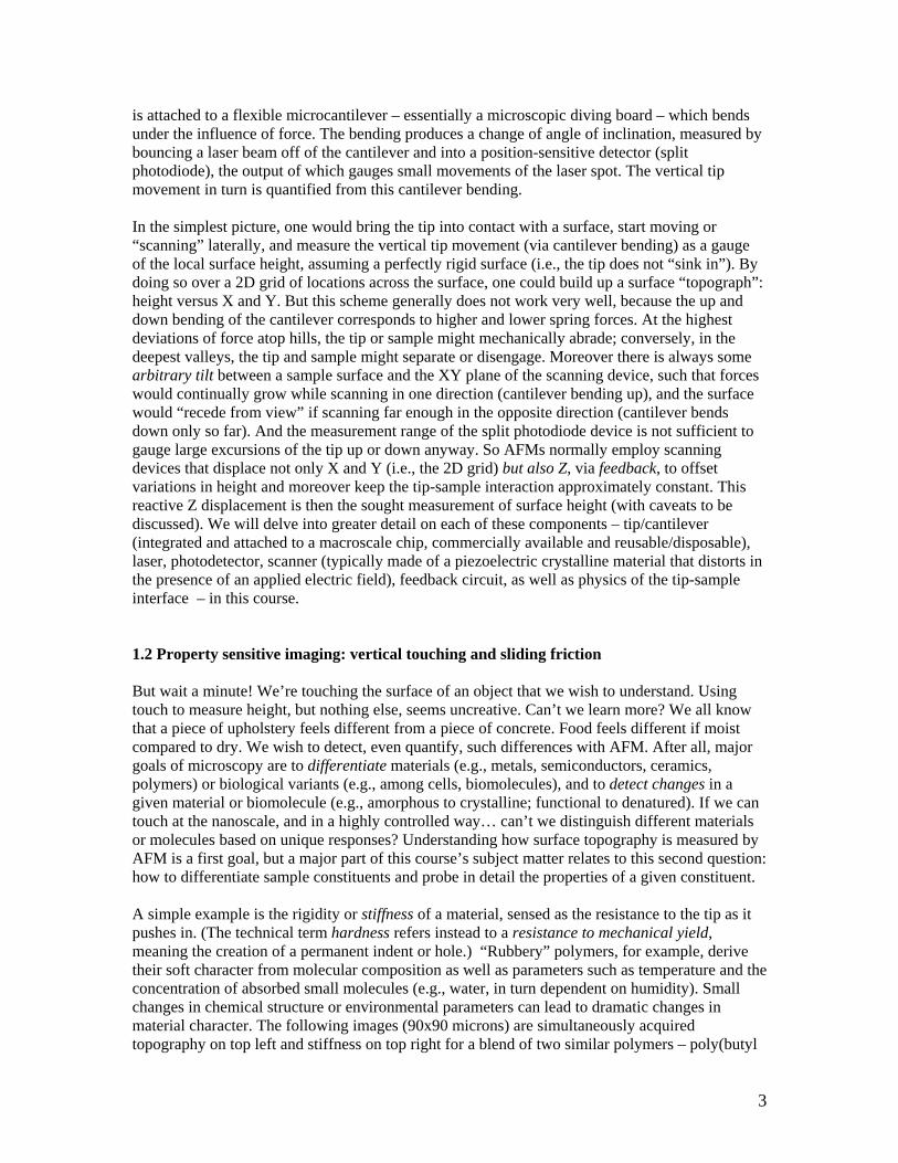
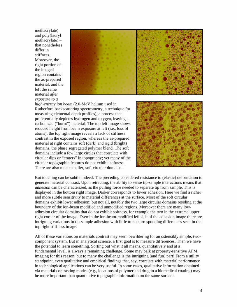
is attached to a flexible microcantilever – essentially a microscopic diving board – which bends under the influence of force. The bending produces a change of angle of inclination, measured by bouncing a laser beam off of the cantilever and into a position-sensitive detector (split photodiode), the output of which gauges small movements of the laser spot. The vertical tip movement in turn is quantified from this cantilever bending. In the simplest picture, one would bring the tip into contact with a surface, start moving or “scanning” laterally, and measure the vertical tip movement (via cantilever bending) as a gauge of the local surface height, assuming a perfectly rigid surface (i.e., the tip does not “sink in”). By doing so over a 2D grid of locations across the surface, one could build up a surface “topograph”: height versus X and Y. But this scheme generally does not work very well, because the up and down bending of the cantilever corresponds to higher and lower spring forces. At the highest deviations of force atop hills, the tip or sample might mechanically abrade; conversely, in the deepest valleys, the tip and sample might separate or disengage. Moreover there is always some arbitrary tilt between a sample surface and the XY plane of the scanning device, such that forces would continually grow while scanning in one direction (cantilever bending up), and the surface would “recede from view” if scanning far enough in the opposite direction (cantilever bends down only so far). And the measurement range of the split photodiode device is not sufficient to gauge large excursions of the tip up or down anyway. So AFMs normally employ scanning devices that displace not only X and Y (i.e., the 2D grid) but also Z, via feedback, to offset variations in height and moreover keep the tip-sample interaction approximately constant. This reactive Z displacement is then the sought measurement of surface height (with caveats to be discussed). We will delve into greater detail on each of these components – tip/cantilever (integrated and attached to a macroscale chip, commercially available and reusable/disposable), laser, photodetector, scanner (typically made of a piezoelectric crystalline material that distorts in the presence of an applied electric field), feedback circuit, as well as physics of the tip-sample interface – in this course. 1.2 Property sensitive imaging: vertical touching and sliding friction But wait a minute! We’re touching the surface of an object that we wish to understand. Using touch to measure height, but nothing else, seems uncreative. Can’t we learn more? We all know that a piece of upholstery feels different from a piece of concrete. Food feels different if moist compared to dry. We wish to detect, even quantify, such differences with AFM. After all, major goals of microscopy are to differentiate materials (e.g., metals, semiconductors, ceramics, polymers) or biological variants (e.g., among cells, biomolecules), and to detect changes in a given material or biomolecule (e.g., amorphous to crystalline; functional to denatured). If we can touch at the nanoscale, and in a highly controlled way… can’t we distinguish different materials or molecules based on unique responses? Understanding how surface topography is measured by AFM is a first goal, but a major part of this course’s subject matter relates to this second question: how to differentiate sample constituents and probe in detail the properties of a given constituent. A simple example is the rigidity or stiffness of a material, sensed as the resistance to the tip as it pushes in. (The technical term hardness refers instead to a resistance to mechanical yield, meaning the creation of a permanent indent or hole.) “Rubbery” polymers, for example, derive their soft character from molecular composition as well as parameters such as temperature and the concentration of absorbed small molecules (e.g., water, in turn dependent on humidity). Small changes in chemical structure or environmental parameters can lead to dramatic changes in material character. The following images (90x90 microns) are simultaneously acquired topography on top left and stiffness on top right for a blend of two similar polymers – poly(butyl

3

methacrylate) and poly(lauryl methacrylate) – that nonetheless differ in stiffness. Moreover, the right portion of the imaged region contains the as-prepared material, and the left the same material after exposure to a high-energy ion beam (2.0-MeV helium used in Rutherford backscattering spectrometry, a technique for measuring elemental depth profiles), a process that preferentially depletes hydrogen and oxygen, leaving a carbonized (“burnt”) material. The top left image shows reduced height from beam exposure at left (i.e., loss of atoms); the top right image reveals a lack of stiffness contrast in the exposed region, whereas the as-prepared material at right contains soft (dark) and rigid (bright) domains, the phase segregated polymer blend. The soft domains include a few large circles that correlate with circular dips or “craters” in topography; yet many of the circular topographic features do not exhibit softness. There are also much smaller, soft circular domains. But touching can be subtle indeed. The preceding considered resistance to (elastic) deformation to generate material contrast. Upon retracting, the ability to sense tip-sample interactions means that adhesion can be characterized, as the pulling force needed to separate tip from sample. This is displayed in the bottom right image. Darker corresponds to lower adhesion. Here we find a richer and more subtle sensitivity to material differences at the surface. Most of the soft circular domains exhibit lower adhesion; but not all, notably the two large circular domains residing at the boundary of the ion-beam modified and unmodified regions. Moreover there are many low-adhesion circular domains that do not exhibit softness, for example the two in the extreme upper right corner of the image. Even in the ion-beam-modified left side of the adhesion image there are intriguing variations in tip-sample adhesion with little to no corresponding differences seen in the top right stiffness image. All of these variations on materials contrast may seem bewildering for an ostensibly simple, two-component system. But in analytical science, a first goal is to measure differences. Then we have the potential to learn something. Sorting out what it all means, quantitatively and at a fundamental level, is always a remaining challenge. Some may balk at property-sensitive AFM imaging for this reason, but to many the challenge is the intriguing (and fun) part! From a utility standpoint, even qualitative and empirical findings that, say, correlate with material performance in technological applications can be very useful. In some cases, qualitative information obtained via material contrasting modes (e.g., locations of polymer and drug in a biomedical coating) may be more important than quantitative topographic information on the same surface.

4

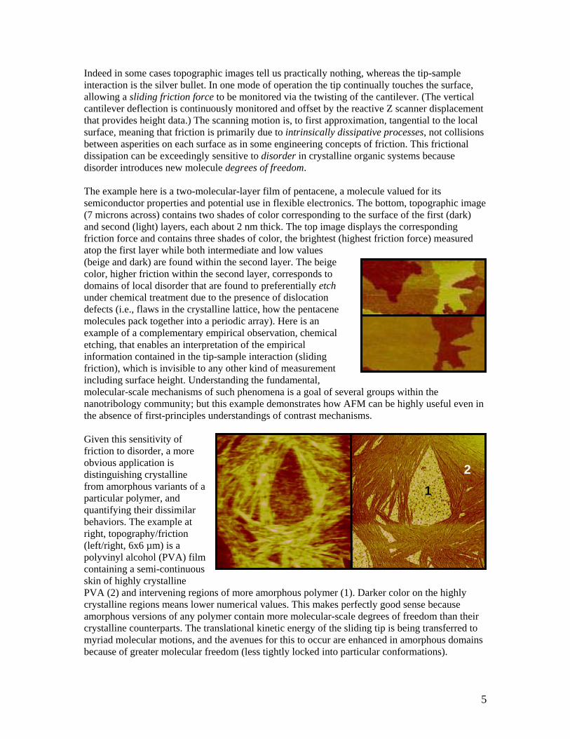
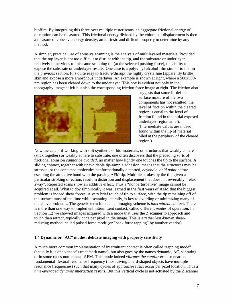
Indeed in some cases topographic images tell us practically nothing, whereas the tip-sample interaction is the silver bullet. In one mode of operation the tip continually touches the surface, allowing a sliding friction force to be monitored via the twisting of the cantilever. (The vertical cantilever deflection is continuously monitored and offset by the reactive Z scanner displacement that provides height data.) The scanning motion is, to first approximation, tangential to the local surface, meaning that friction is primarily due to intrinsically dissipative processes, not collisions between asperities on each surface as in some engineering concepts of friction. This frictional dissipation can be exceedingly sensitive to disorder in crystalline organic systems because disorder introduces new molecule degrees of freedom. The example here is a two-molecular-layer film of pentacene, a molecule valued for its semiconductor properties and potential use in flexible electronics. The bottom, topographic image (7 microns across) contains two shades of color corresponding to the surface of the first (dark) and second (light) layers, each about 2 nm thick. The top image displays the corresponding friction force and contains three shades of color, the brightest (highest friction force) measured atop the first layer while both intermediate and low values (beige and dark) are found within the second layer. The beige color, higher friction within the second layer, corresponds to domains of local disorder that are found to preferentially etch under chemical treatment due to the presence of dislocation defects (i.e., flaws in the crystalline lattice, how the pentacene molecules pack together into a periodic array). Here is an example of a complementary empirical observation, chemical etching, that enables an interpretation of the empirical information contained in the tip-sample interaction (sliding friction), which is invisible to any other kind of measurement including surface height. Understanding the fundamental, molecular-scale mechanisms of such phenomena is a goal of several groups within the nanotribology community; but this example demonstrates how AFM can be highly useful even in the absence of first-principles understandings of contrast mechanisms. Given this sensitivity of friction to disorder, a more obvious application is distinguishing crystalline from amorphous variants of a particular polymer, and quantifying their dissimilar behaviors. The example at right, topography/friction (left/right, 6x6 µm) is a polyvinyl alcohol (PVA) film containing a semi-continuous skin of highly crystalline PVA (2) and intervening regions of more amorphous polymer (1). Darker color on the highly crystalline regions means lower numerical values. This makes perfectly good sense because amorphous versions of any polymer contain more molecular-scale degrees of freedom than their crystalline counterparts. The translational kinetic energy of the sliding tip is being transferred to myriad molecular motions, and the avenues for this to occur are enhanced in amorphous domains because of greater molecular freedom (less tightly locked into particular conformations).

21

5

A broad strength of AFM is the capacity for environmental control. Humidity can have profound effects on friction, and indeed on the properties of the material being probed via frictional imaging. The graph at left compares the humidity dependence of the highly crystalline(2) and more amorphous domain the preceding images. We see thathis dependence is quite flat on the highly crystalline domains up throug75% relative humidity, whereas it exhibits a steep increase above 60% on the more amorphous domains. Raising humidity causes water molecules to be absorbed into

amorphous domains in (water-soluble) polymer matrices, thereby “plasticizing” the polymer to enhance molecular motion, and thus elevate friction. Indeed it is well known that even a “soinduced” glass-to-rubber transition can result, whereby the solid transitions from a rigid plastican easily deformable rubber. The glass-to-rubber transition temperature (Tg) for anhydrous PVA is many tens of degrees above room temperature, meaning that the absorbed water in domains #1 at 75% RH has effectively decreased Tg by many tens of degrees, a truly dramatic change in material properties. Thus one can imagine using friction force AFM as a gauge of small-molecabsorption into polym

ins (1)

t

h

lvent- to

ule eric matrices.

000 20 40 60 80 1

Fric

tiona

l For

ce (n

N)

Relative Humidity (%)

0

20

40

60

80

100

120

1

20 20 40 60 80 100

Fric

tiona

l For

ce (n

N)

Relative Humidity (%)

0

20

40

60

80

100

120

1

2

1.3. Disrupting the surface with a sliding tip Shear forces also can be used to “tear up” a material. This approach has found utility in the biological as well as synthetic material realms. One example is a method to quantify cohesive strength of biofilms, specifically the extracellular polymer substances (proteins, polysaccharides) that serve as a “glue” to bind together a matrix containing bacterial cells, in the case of waste water treatment biofilms. (Cohesion in and adhesion of biofilms is of great significance to many technological applications, whether this mechanical integrity is desirable or undesirable.) With successive raster scans at relatively high loading forces, a gradual excavation of the matrix takes place, whereby molecules are displaced by shear forces. During the course of this multi-raster process, one can reduce the loading (vertical) force to avoid abrasion, zoom out and acquire topographic images to assess the previous excavation process (rightmost image, 3.7x3.7 µm). Comparison with an initial image of the pristine surface (left image) can be made to quantify the abraded surface. In particular one can compute the volume of material displaced by abrasive scanning. It is also possible to analyze the total friction force versus load to identify the fraction of frictional energy transfer that is responsible for abrading the

6

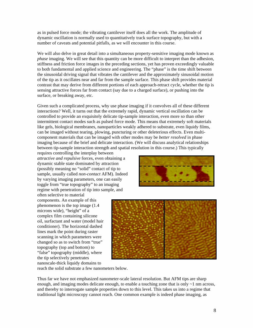
biofilm. By integrating this force over multiple raster scans, an aggregate frictional energy of disruption can be measured. This frictional energy divided by the volume of displacement is then a measure of cohesive energy density, an intrinsic and difficult property to determine by any method. A simpler, practical use of abrasive scanning is the analysis of multilayered materials. Provided that the top layer is not too difficult to disrupt with the tip, and the substrate or underlayer relatively impervious to this same scanning tip (at the selected pushing force), the ability to expose the substrate or underlayer results. One case is a polyvinyl alcohol film similar to that in the previous section. It is quite easy to fracture/disrupt the highly crystalline (apparently brittle) skin and expose a more amorphous underlayer. An example is shown at right, where a 500x500-nm region has been cleared down to the underlayer. This box is evident not only in the topography image at left but also the corresponding friction force image at right. The friction also

suggests that some ill-defined surface mixture of the two components has not resulted: the level of friction within the cleared region is equal to the level of friction found in the initial exposed underlayer region at left. (Intermediate values are indeed found within the lip of material piled at the periphery of the cleared region.)

Now the catch: if working with soft synthetic or bio-materials, or structures that weakly cohere (stick together) or weakly adhere to substrate, one often discovers that the preceding sorts of frictional abrasion cannot be avoided, no matter how lightly one touches the tip to the surface. A sliding contact, together with unavoidable tip-sample adhesion, means that the structures may be stressed, or the contacted molecules conformationally distorted, beyond a yield point before escaping the attractive bond with the passing AFM tip. Multiple strokes by the tip, given a particular stroking direction, result in distortion and displacement that does not reversibly “relax away”. Repeated scans show an additive effect. Thus a “nonperturbative” image cannot be acquired at all. What to do? Empirically it was learned in the first years of AFM that the biggest problem is indeed shear forces. A very brief touch of tip to surface, with the tip remaining off of the surface most of the time while scanning laterally, is key to avoiding or minimizing many of the above problems. The generic term for such an imaging scheme is intermittent contact. There is more than one way to implement intermittent contact, called different modes of operation. In Section 1.2 we showed images acquired with a mode that uses the Z scanner to approach and touch then retract, typically once per pixel in the image. This is a rather less-known shear-reducing method, called pulsed force mode (or “peak force tapping” by another vendor). 1.4 Dynamic or “AC” modes: delicate imaging with property sensitivity A much more common implementation of intermittent contact is often called “tapping mode” (actually it is one vendor’s trademark name), but also goes by the names dynamic, AC, vibrating, or in some cases non-contact AFM. This mode indeed vibrates the cantilever at or near its fundamental flexural resonance frequency (most diving board-shaped objects have multiple resonance frequencies) such that many cycles of approach-retract occur per pixel location. Thus a time-averaged dynamic interaction results. But this vertical cycle is not actuated by the Z scanner

7

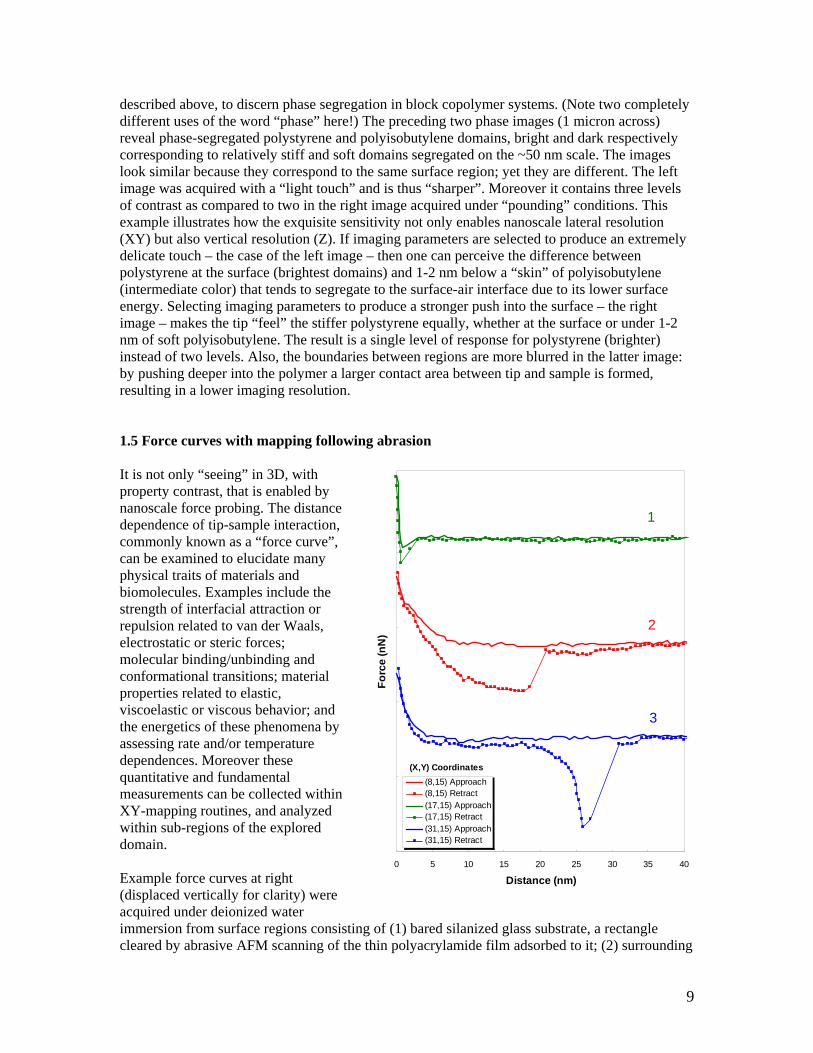
as in pulsed force mode; the vibrating cantilever itself does all the work. The amplitude of dynamic oscillation is normally used to quantitatively track surface topography, but with a number of caveats and potential pitfalls, as we will encounter in this course. We will also delve in great detail into a simultaneous property-sensitive imaging mode known as phase imaging. We will see that this quantity can be more difficult to interpret than the adhesion, stiffness and friction force images in the preceding sections, yet has proven exceedingly valuable to both fundamental and applied science and engineering. The “phase” is the time shift between the sinusoidal driving signal that vibrates the cantilever and the approximately sinusoidal motion of the tip as it oscillates near and far from the sample surface. This phase shift provides material contrast that may derive from different portions of each approach-retract cycle, whether the tip is sensing attractive forces far from contact (say due to a charged surface), or pushing into the surface, or breaking away, etc. Given such a complicated process, why use phase imaging if it convolves all of these different interactions? Well, it turns out that the extremely rapid, dynamic vertical oscillation can be controlled to provide an exquisitely delicate tip-sample interaction, even more so than other intermittent contact modes such as pulsed force mode. This means that extremely soft materials like gels, biological membranes, nanoparticles weakly adhered to substrate, even liquidy films, can be imaged without tearing, plowing, puncturing or other deleterious effects. Even multi-component materials that can be imaged with other modes may be better resolved in phase imaging because of the brief and delicate interaction. (We will discuss analytical relationships between tip-sample interaction strength and spatial resolution in this course.) This typically requires controlling the interplay between attractive and repulsive forces, even obtaining a dynamic stable state dominated by attraction (possibly meaning no “solid” contact of tip to sample, usually called non-contact AFM). Indeed by varying imaging parameters, one can easily toggle from “true topography” to an imaging regime with penetration of tip into sample, and often selective to material components. An example of this phenomenon is the top image (1.4 microns wide), “height” of a complex film containing silicone oil, surfactant and water (model hair conditioner). The horizontal dashed lines mark the point during raster scanning in which parameters were changed so as to switch from “true” topography (top and bottom) to “false” topography (middle), where the tip selectively penetrates nanoscale-thick liquidy domains to reach the solid substrate a few nanometers below. Thus far we have not emphasized nanometer-scale lateral resolution. But AFM tips are sharp enough, and imaging modes delicate enough, to enable a touching zone that is only ~1 nm across, and thereby to interrogate sample properties down to this level. This takes us into a regime that traditional light microscopy cannot reach. One common example is indeed phase imaging, as

8

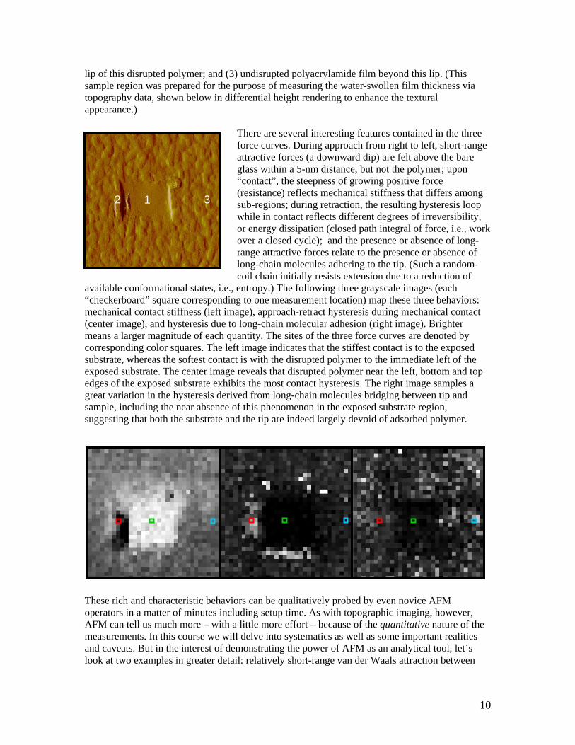
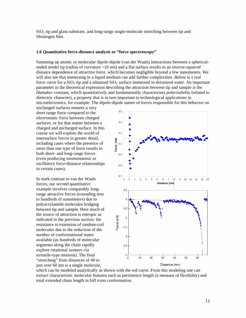
described above, to discern phase segregation in block copolymer systems. (Note two completely different uses of the word “phase” here!) The preceding two phase images (1 micron across) reveal phase-segregated polystyrene and polyisobutylene domains, bright and dark respectively corresponding to relatively stiff and soft domains segregated on the ~50 nm scale. The images look similar because they correspond to the same surface region; yet they are different. The left image was acquired with a “light touch” and is thus “sharper”. Moreover it contains three levels of contrast as compared to two in the right image acquired under “pounding” conditions. This example illustrates how the exquisite sensitivity not only enables nanoscale lateral resolution (XY) but also vertical resolution (Z). If imaging parameters are selected to produce an extremely delicate touch – the case of the left image – then one can perceive the difference between polystyrene at the surface (brightest domains) and 1-2 nm below a “skin” of polyisobutylene (intermediate color) that tends to segregate to the surface-air interface due to its lower surface energy. Selecting imaging parameters to produce a stronger push into the surface – the right image – makes the tip “feel” the stiffer polystyrene equally, whether at the surface or under 1-2 nm of soft polyisobutylene. The result is a single level of response for polystyrene (brighter) instead of two levels. Also, the boundaries between regions are more blurred in the latter image: by pushing deeper into the polymer a larger contact area between tip and sample is formed, resulting in a lower imaging resolution. 1.5 Force curves with mapping following abrasion It is not only “seeing” in 3D, with property contrast, that is enabled by nanoscale force probing. The distance dependence of tip-sample interaction, commonly known as a “force curve”, can be examined to elucidate many physical traits of materials and biomolecules. Examples include the strength of interfacial attraction or repulsion related to van der Waals, electrostatic or steric forces; molecular binding/unbinding and conformational transitions; material properties related to elastic, viscoelastic or viscous behavior; and the energetics of these phenomena by assessing rate and/or temperature dependences. Moreover these quantitative and fundamental measurements can be collected within XY-mapping routines, and analyzed within sub-regions of the explored domain. Example force curves at right (displaced vertically for clarity) were acquired under deionized water immersion from surface regions consisting of (1) bared silanized glass substrate, a rectangle cleared by abrasive AFM scanning of the thin polyacrylamide film adsorbed to it; (2) surrounding

0 5 10 15 20 25 30 35 40

Distance (nm)

Forc

e (n

N)

(8,15) Approach(8,15) Retract(17,15) Approach(17,15) Retract(31,15) Approach(31,15) Retract

(X,Y) Coordinates

1

2

3

9

lip of this disrupted polymer; and (3) undisrupted polyacrylamide film beyond this lip. (This sample region was prepared for the purpose of measuring the water-swollen film thickness vtopography data, shown below in di

ia fferential height rendering to enhance the textural

appearance.)

e

upon

rk

of

act

and

suggesting that both the substrate and the tip are indeed largely devoid of adsorbed polymer.

look at two examples in greater detail: relatively short-range van der Waals attraction between

There are several interesting features contained in the three force curves. During approach from right to left, short-rangattractive forces (a downward dip) are felt above the bareglass within a 5-nm distance, but not the polymer; “contact”, the steepness of growing positive force (resistance) reflects mechanical stiffness that differs among sub-regions; during retraction, the resulting hysteresis loop while in contact reflects different degrees of irreversibility, or energy dissipation (closed path integral of force, i.e., woover a closed cycle); and the presence or absence of long-range attractive forces relate to the presence or absence of long-chain molecules adhering to the tip. (Such a random-coil chain initially resists extension due to a reduction

available conformational states, i.e., entropy.) The following three grayscale images (each “checkerboard” square corresponding to one measurement location) map these three behaviors: mechanical contact stiffness (left image), approach-retract hysteresis during mechanical cont(center image), and hysteresis due to long-chain molecular adhesion (right image). Brighter means a larger magnitude of each quantity. The sites of the three force curves are denoted by corresponding color squares. The left image indicates that the stiffest contact is to the exposed substrate, whereas the softest contact is with the disrupted polymer to the immediate left of the exposed substrate. The center image reveals that disrupted polymer near the left, bottom and top edges of the exposed substrate exhibits the most contact hysteresis. The right image samples a great variation in the hysteresis derived from long-chain molecules bridging between tip sample, including the near absence of this phenomenon in the exposed substrate region,

These rich and characteristic behaviors can be qualitatively probed by even novice AFM operators in a matter of minutes including setup time. As with topographic imaging, however, AFM can tell us much more – with a little more effort – because of the quantitative nature of the measurements. In this course we will delve into systematics as well as some important realitiesand caveats. But in the interest of demonstrating the power of AFM as an analytical tool, let’s

1 2 3

10

SiO2 tip and glass substrate, and long-range single-molecule stretching between tip and fibrinogen film. 1.6 Quantitative force-distance analysis or “force spectroscopy” Summing up atomic or molecular dipole-dipole (van der Waals) interactions between a spherical-ended model tip (radius of curvature ~10 nm) and a flat surface results in an inverse-squared distance dependence of attractive force, which becomes negligible beyond a few nanometers. We will also see that immersing in a liquid medium can add further complexities. Below is a real force curve for a SiO2 tip and a silanized SiO2 surface immersed in deionized water. An important parameter in the theoretical expression describing the attraction between tip and sample is the Hamaker constant, which quantitatively and fundamentally characterizes polarizability (related to dielectric character), a property that is in turn important to technological applications in microelectronics, for example. The dipole-dipole nature of forces responsible for this behavior on uncharged surfaces ensures a very short range force compared to the electrostatic force between charged surfaces, or for that matter between a charged and uncharged surface. In this course we will explore the world of intersurface forces in greater detail, including cases where the presence of more than one type of force results in both short- and long-range forces (even producing nonmonotonic or oscillatory force-distance relationships in certain cases). In stark contrast to van der Waals forces, our second quantitative example involves comparably long-range attractive forces (extending tens to hundreds of nanometers) due to polyacrylamide molecules bridging between tip and sample. Here much of the source of attraction is entropic as indicated in the previous section: the resistance to extension of random-coil molecules due to the reduction of the number of conformational states available (as hundreds of molecular segments along the chain rapidly explore rotational isomers via turnstile-type motions). The final “stretching” from distances of 40 to just over 60 nm is a single molecule, which can be modeled analytically as shown with the red curve. From this modeling one can extract characteristic molecular features such as persistence length (a measure of flexibility) and total extended chain length in full trans conformation.

-0.7

-0.5

-0.3

-0.1

0.1

0.3

0.5

-1 0 1 2 3 4 5 6 7 8 9 10 11 12 13 14

Distance (nm)

Forc

e (n

N)

11

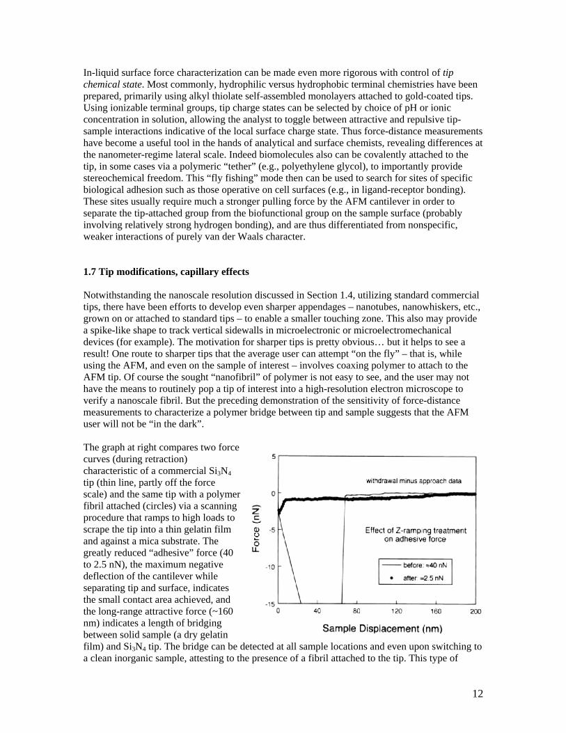
In-liquid surface force characterization can be made even more rigorous with control of tip chemical state. Most commonly, hydrophilic versus hydrophobic terminal chemistries have been prepared, primarily using alkyl thiolate self-assembled monolayers attached to gold-coated tips. Using ionizable terminal groups, tip charge states can be selected by choice of pH or ionic concentration in solution, allowing the analyst to toggle between attractive and repulsive tip-sample interactions indicative of the local surface charge state. Thus force-distance measurements have become a useful tool in the hands of analytical and surface chemists, revealing differences at the nanometer-regime lateral scale. Indeed biomolecules also can be covalently attached to the tip, in some cases via a polymeric “tether” (e.g., polyethylene glycol), to importantly provide stereochemical freedom. This “fly fishing” mode then can be used to search for sites of specific biological adhesion such as those operative on cell surfaces (e.g., in ligand-receptor bonding). These sites usually require much a stronger pulling force by the AFM cantilever in order to separate the tip-attached group from the biofunctional group on the sample surface (probably involving relatively strong hydrogen bonding), and are thus differentiated from nonspecific, weaker interactions of purely van der Waals character. 1.7 Tip modifications, capillary effects Notwithstanding the nanoscale resolution discussed in Section 1.4, utilizing standard commercial tips, there have been efforts to develop even sharper appendages – nanotubes, nanowhiskers, etc., grown on or attached to standard tips – to enable a smaller touching zone. This also may provide a spike-like shape to track vertical sidewalls in microelectronic or microelectromechanical devices (for example). The motivation for sharper tips is pretty obvious… but it helps to see a result! One route to sharper tips that the average user can attempt “on the fly” – that is, while using the AFM, and even on the sample of interest – involves coaxing polymer to attach to the AFM tip. Of course the sought “nanofibril” of polymer is not easy to see, and the user may not have the means to routinely pop a tip of interest into a high-resolution electron microscope to verify a nanoscale fibril. But the preceding demonstration of the sensitivity of force-distance measurements to characterize a polymer bridge between tip and sample suggests that the AFM user will not be “in the dark”. The graph at right compares two force curves (during retraction) characteristic of a commercial Si3N4 tip (thin line, partly off the force scale) and the same tip with a polymer fibril attached (circles) via a scanning procedure that ramps to high loads to scrape the tip into a thin gelatin film and against a mica substrate. The greatly reduced “adhesive” force (40 to 2.5 nN), the maximum negative deflection of the cantilever while separating tip and surface, indicates the small contact area achieved, and the long-range attractive force (~160 nm) indicates a length of bridging between solid sample (a dry gelatin film) and Si3N4 tip. The bridge can be detected at all sample locations and even upon switching to a clean inorganic sample, attesting to the presence of a fibril attached to the tip. This type of

12

modified tip is not uselessly transient; it can be stable over the course of many images and even if using the tip to image several samples. Comparing images of a gelatin film before and after (left/right) this tip modification, one finds a transformation from “granular” images to a fibrous image. The ratio of grain size in the left image to fiber diameter in the right image is approximately the same as the ratio of tip-sample adhesive forces at the initial break of contact, consistent with the concept of a scaled down contact area. A fibrous morphology is what one expects given nanoscale resolution: gelatin derives from the connective protein collagen that naturally forms a hierarchy of fibrous structures ranging down to the nanoscale in diameter.

30 nm

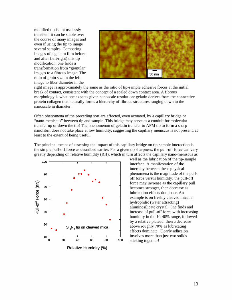
Often phenomena of the preceding sort are affected, even actuated, by a capillary bridge or “nano-meniscus” between tip and sample. This bridge may serve as a conduit for molecular transfer up or down the tip! The phenomenon of gelatin transfer to AFM tip to form a sharp nanofibril does not take place at low humidity, suggesting the capillary meniscus is not present, at least to the extent of being useful. The principal means of assessing the impact of this capillary bridge on tip-sample interaction is the simple pull-off force as described earlier. For a given tip sharpness, the pull-off force can vary greatly depending on relative humidity (RH), which in turn affects the capillary nano-meniscus as

well as the lubrication of the tip-sample interface. A manifestation of the interplay between these physical phenomena is the magnitude of the pull-off force versus humidity: the pull-off force may increase as the capillary pull becomes stronger, then decrease as lubrication effects dominate. An example is on freshly cleaved mica, a hydrophilic (water attracting) aluminosilicate crystal. One finds and increase of pull-off force with increasing humidity in the 10-40% range, followed by a relative plateau, then a decrease above roughly 70% as lubricating effects dominate. Clearly adhesion involves more than just two solids sticking together!

40

50

60

70

80

90

100

0 20 40 60 80 10

Relative Humidity (%)

Pul

l-off

Forc

e (n

N)

Si3N4 tip on cleaved mica

040

50

60

70

80

90

100100

0 20 40 60 80 10

Relative Humidity (%)

Pul

l-off

Forc

e (n

N)

Si3N4 tip on cleaved mica

0

13

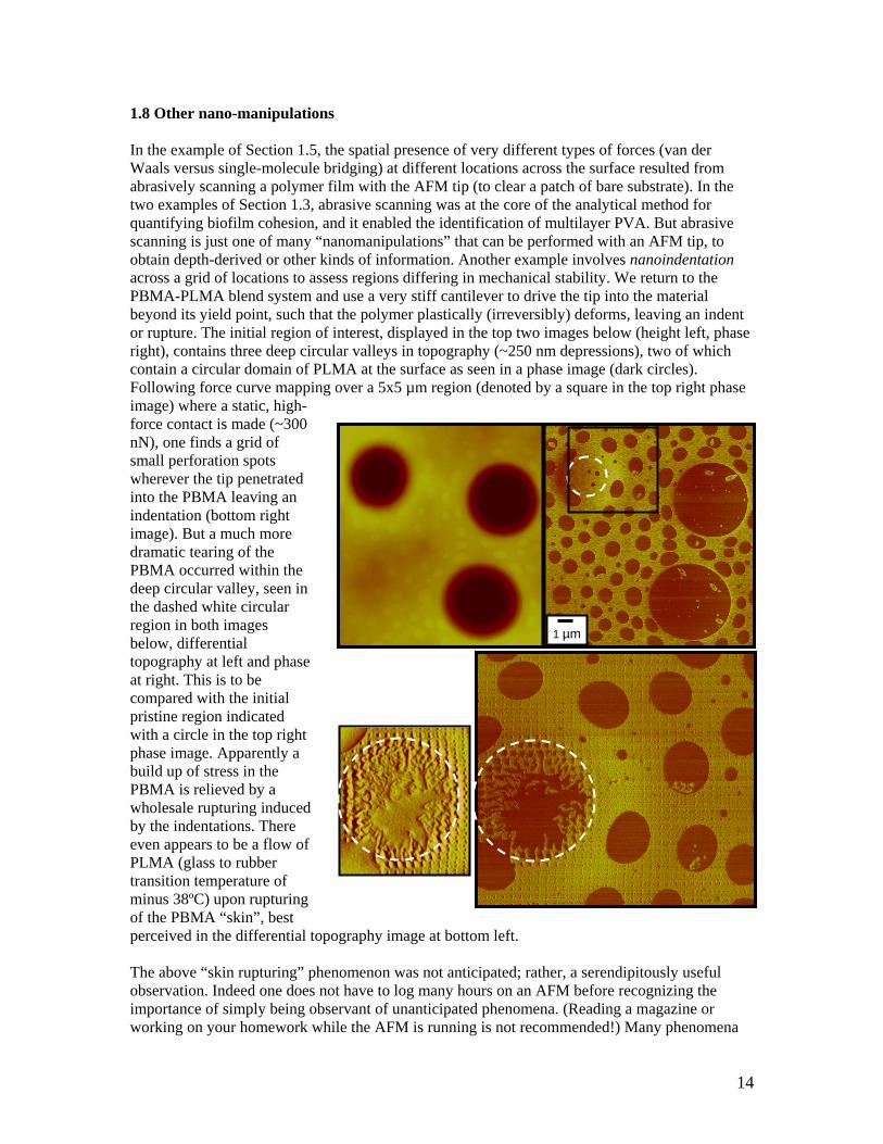
1.8 Other nano-manipulations In the example of Section 1.5, the spatial presence of very different types of forces (van der Waals versus single-molecule bridging) at different locations across the surface resulted from abrasively scanning a polymer film with the AFM tip (to clear a patch of bare substrate). In the two examples of Section 1.3, abrasive scanning was at the core of the analytical method for quantifying biofilm cohesion, and it enabled the identification of multilayer PVA. But abrasive scanning is just one of many “nanomanipulations” that can be performed with an AFM tip, to obtain depth-derived or other kinds of information. Another example involves nanoindentation across a grid of locations to assess regions differing in mechanical stability. We return to the PBMA-PLMA blend system and use a very stiff cantilever to drive the tip into the material beyond its yield point, such that the polymer plastically (irreversibly) deforms, leaving an indent or rupture. The initial region of interest, displayed in the top two images below (height left, phase right), contains three deep circular valleys in topography (~250 nm depressions), two of which contain a circular domain of PLMA at the surface as seen in a phase image (dark circles). Following force curve mapping over a 5x5 µm region (denoted by a square in the top right phase image) where a static, high-force contact is made (~300 nN), one finds a grid of small perforation spots wherever the tip penetrated into the PBMA leaving an indentation (bottom right image). But a much more dramatic tearing of the PBMA occurred within the deep circular valley, seen in the dashed white circular region in both images below, differential topography at left and phase at right. This is to be compared with the initial pristine region indicated with a circle in the top right phase image. Apparently a build up of stress in the PBMA is relieved by a wholesale rupturing iby the indentations. There even appears to be a flow ofPLMA (glass to rubber transition temperaminus 38ºC) upon rupturing of the PBMA “skin”, bperceived in the differential topography image at bottom left.

1 µm

nduced

ture of

est

The above “skin rupturing” phenomenon was not anticipated; rather, a serendipitously useful observation. Indeed one does not have to log many hours on an AFM before recognizing the importance of simply being observant of unanticipated phenomena. (Reading a magazine or working on your homework while the AFM is running is not recommended!) Many phenomena

14

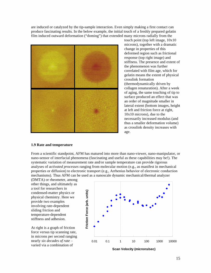
are induced or catalyzed by the tip-sample interaction. Even simply making a first contact can produce fascinating results. In the below example, the initial touch of a freshly prepared gelatin film induced outward deformation (“doming”) that extended many microns radially from the

touch point (top left image, 10x10 microns), together with a dramatic change in properties of this deformed region such as frictional response (top right image) and stiffness. The presence and extent of the phenomenon was further correlated with film age, which for gelatin means the extent of physical crosslink formation (thermodynamically driven by collagen renaturation). After a week of aging, the same touching of tip to surface produced an effect that was an order of magnitude smaller in lateral extent (bottom images, height at left and friction force at right, 10x10 microns), due to the necessarily increased modulus (and thus a smaller deformation volume) as crosslink density increases with age.

1.9 Rate and temperature From a scientific standpoint, AFM has matured into more than nano-viewer, nano-manipulator, or nano-sensor of interfacial phenomena (fascinating and useful as these capabilities may be!). The systematic variation of measurement rate and/or sample temperature can provide rigorous analyses of activated processes ranging from molecular motion (e.g., as manifest in mechanical properties or diffusion) to electronic transport (e.g., Arrhenius behavior of electronic conduction mechanisms). Thus AFM can be used as a nanoscale dynamic mechanical/thermal analyzer (DMTA) or rheometer, among other things, and ultimately as a tool for researchers in condensed-matter physics or physical chemistry. Here we provide two examples involving rate-dependent sliding friction and temperature-dependent stiffness and adhesion.

0.01 0.1 1 10 100 1000 10000

Scan Velocity (microns/sec)

Fric

tion

Forc

e (a

rb. u

nits

)

At right is a graph of friction force versus tip scanning rate, in microns per second ranging nearly six decades of rate – varied via a combination of

15

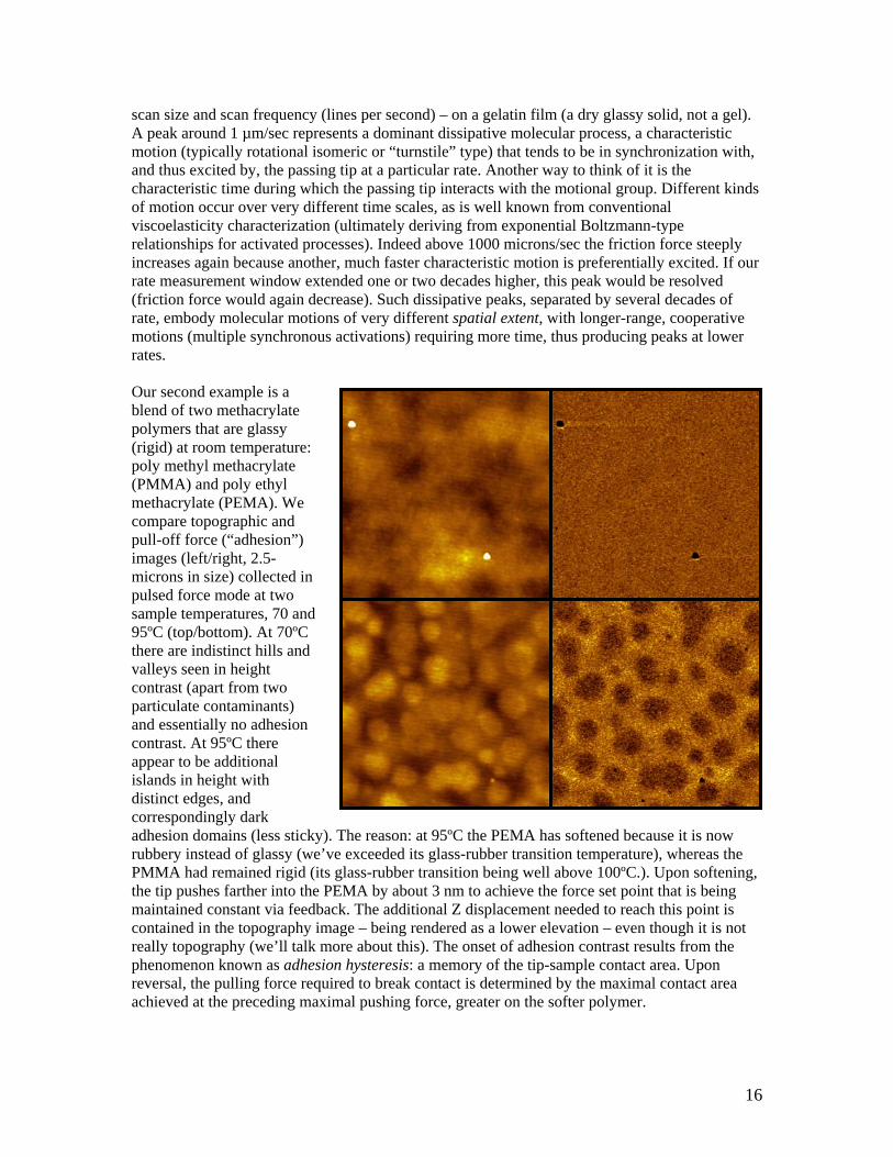
scan size and scan frequency (lines per second) – on a gelatin film (a dry glassy solid, not a gel). A peak around 1 µm/sec represents a dominant dissipative molecular process, a characteristic motion (typically rotational isomeric or “turnstile” type) that tends to be in synchronization with, and thus excited by, the passing tip at a particular rate. Another way to think of it is the characteristic time during which the passing tip interacts with the motional group. Different kinds of motion occur over very different time scales, as is well known from conventional viscoelasticity characterization (ultimately deriving from exponential Boltzmann-type relationships for activated processes). Indeed above 1000 microns/sec the friction force steeply increases again because another, much faster characteristic motion is preferentially excited. If our rate measurement window extended one or two decades higher, this peak would be resolved (friction force would again decrease). Such dissipative peaks, separated by several decades of rate, embody molecular motions of very different spatial extent, with longer-range, cooperative motions (multiple synchronous activations) requiring more time, thus producing peaks at lower rates. Our second example is a blend of two methacrylate polymers that are glassy (rigid) at room temperature: poly methyl methacrylate (PMMA) and poly ethyl methacrylate (PEMA). We compare topographic and pull-off force (“adhesion”) images (left/right, 2.5-microns in size) collected in pulsed force mode at two sample temperatures, 70 and 95ºC (top/bottom). At 70ºC there are indistinct hills and valleys seen in height contrast (apart from two particulate contaminants) and essentially no adhesion contrast. At 95ºC there appear to be additional islands in height with distinct edges, and correspondingly dark adhesion domains (less sticky). The reason: at 95ºC the PEMA has softened because it is now rubbery instead of glassy (we’ve exceeded its glass-rubber transition temperature), whereas the PMMA had remained rigid (its glass-rubber transition being well above 100ºC.). Upon softening, the tip pushes farther into the PEMA by about 3 nm to achieve the force set point that is being maintained constant via feedback. The additional Z displacement needed to reach this point is contained in the topography image – being rendered as a lower elevation – even though it is not really topography (we’ll talk more about this). The onset of adhesion contrast results from the phenomenon known as adhesion hysteresis: a memory of the tip-sample contact area. Upon reversal, the pulling force required to break contact is determined by the maximal contact area achieved at the preceding maximal pushing force, greater on the softer polymer.

16

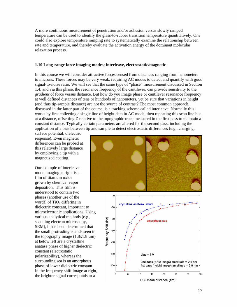
A more continuous measurement of penetration and/or adhesion versus slowly ramped temperature can be used to identify the glass-to-rubber transition temperature quantitatively. One could also explore temperature ramping rate to systematically examine the relationship between rate and temperature, and thereby evaluate the activation energy of the dominant molecular relaxation process. 1.10 Long-range force imaging modes; interleave, electrostatic/magnetic In this course we will consider attractive forces sensed from distances ranging from nanometers to microns. These forces may be very weak, requiring AC modes to detect and quantify with good signal-to-noise ratio. We will see that the same type of “phase” measurement discussed in Section 1.4, and via this phase, the resonance frequency of the cantilever, can provide sensitivity to the gradient of force versus distance. But how do you image phase or cantilever resonance frequency at well defined distances of tens or hundreds of nanometers, yet be sure that variations in height (and thus tip-sample distance) are not the source of contrast? The most common approach, discussed in the latter part of the course, is a tracking scheme called interleave. Normally this works by first collecting a single line of height data in AC mode, then repeating this scan line but at a distance, offsetting Z relative to the topographic trace measured in the first pass to maintain a constant distance. Typically certain parameters are altered for the second pass, including the application of a bias between tip and sample to detect electrostatic differences (e.g., charging, surface potential, dielectric response). Even magnetic differences can be probed at this relatively large distance by employing a tip with a magnetized coating. Our example of interleave mode imaging at right is a film of titanium oxide grown by chemical vapor deposition. This film is understood to contain two phases (another use of the word!) of TiO2 differing in dielectric constant, important to microelectronic applications. Using various analytical methods (e.g., scanning electron microscopy, SEM), it has been determined that the small protruding islands seen in the topography image (1.8x1.8 µm) at below left are a crystalline anatase phase of higher dielectric constant (electrostatic polarizability), whereas the surrounding sea is an amorphous phase of lower dielectric constant. In the frequency shift image at right, the brighter signal corresponds to a

17

18

less negative shift of the cantilever’s resonant frequency (meaning a weaker attractive force gradient) during the interleave pass at about 6 nm mean distance between tip and sample. This type of image was repeatedly collected at a number of distances, and the resonant frequency shifts plotted below comparing two surface locations: centered above a crystalline anatase island (blue) and above the sea far from any island. The curves are guides to the eye. At any given distance the attractive force gradient is about 50% stronger above the sea, a rather surprising result at first sight. But computer simulations of this electrostatics problem unveiled that the topography of the surface, as well as the subsurface morphology of the grain and sea (determined from cross-sectional scanning electron microscopy), is essential to understand this result. At this stage the important messages are (1) exquisite sensitivity that enables long-range force detection via shifts of the cantilever’s resonant frequency; (2) the ability to precisely control the tip-sample distance maintained during interleave imaging, and vary systematically from image to image; (3) the sensitivity of this measurement to both electromagnetic properties and morphology, and the concomitant importance of modeling to sort out competing factors.