000 Received: xxxxxxxx / Accepted: xxxxxxxx / Published online: xxxxxxxx thermal effects, simulation, machine tool, environment, positioning errors Dr.-Ing. Janine Glänzel 1Andreas Naumann 2 Tharun Suresh Kumar 1*PARALLEL COMPUTING IN AUTOMATION OF DECOUPLED FLUID- THERMOSTRUCTURAL SIMULATION APPROACH Decoupling approach presents a novel solution/alternative to the highly time-consuming fluid- thermal-structural simulation procedures when thermal effects and resultant displacements on machine tools are analyzed. Using high dimensional Characteristic Diagrams (CDs) along with a Clustering Algorithm that immensely reduces the data needed for training, a limited number of CFD simulations can suffice in effectively decoupling fluid and thermal-structural simulations. This approach becomes highly significant when complex geometries or dynamic components are considered. However, there is still scope for improvement in the reduction of time needed to train CDs. Parallel computation can be effectively utilized in decoupling approach in simultaneous execution of (i) CFD simulations and data export, and (ii) Clustering technique involving Genetic Algorithm and Radial Basis Function interpolation, which clusters and optimizes the training data for CDs. Parallelization reduces the entire computation duration from several days to a few hours and thereby, improving the efficiency and ease-of- use of decoupling simulation approach. 1. INTRODUCTION When a machine tool is subjected to changes in environmental influences such as ambient air temperature, velocity or direction, then flow (CFD) simulations are necessary to effectively quantify the thermal behaviour between the machine tool surface and the surrounding air (fluid), ref Glänzel et al. [1]. This two-step simulation procedure involving fluid and thermo-structural simulations is highly complex and time-consuming especially when complex geometries or dynamic components are considered. Reducing the dependency of thermo-structural simulations on CFD simulations for convection data is a matter of great concern as far as reduction in computation time is concerned. A suitable alternative for the above process can be attained by decoupling CFD and thermo-structural simulations .This can be achieved by introducing a clustering algorithm (CA) and characteristic diagrams (CDs) in the workflow. 1 Fraunhofer Institute for Machine Tools and Forming Technology IWU Chemnitz, Germany 2 Dresden University of Technology, Institute of Scientific Computing, Dresden, Germany * E-Mail: [email protected]DOI: xxxxxxxx ,
Transcript
000
Received: xxxxxxxx / Accepted: xxxxxxxx / Published online: xxxxxxxx
thermal effects, simulation,
machine tool, environment,
positioning errors
Dr.-Ing. Janine Glänzel1
Andreas Naumann2
Tharun Suresh Kumar 1*
PARALLEL COMPUTING IN AUTOMATION OF DECOUPLED FLUID-
THERMOSTRUCTURAL SIMULATION APPROACH
Decoupling approach presents a novel solution/alternative to the highly time-consuming fluid- thermal-structural
simulation procedures when thermal effects and resultant displacements on machine tools are analyzed. Using
high dimensional Characteristic Diagrams (CDs) along with a Clustering Algorithm that immensely reduces the
data needed for training, a limited number of CFD simulations can suffice in effectively decoupling fluid and
thermal-structural simulations. This approach becomes highly significant when complex geometries or dynamic
components are considered. However, there is still scope for improvement in the reduction of time needed to
train CDs. Parallel computation can be effectively utilized in decoupling approach in simultaneous execution of
(i) CFD simulations and data export, and (ii) Clustering technique involving Genetic Algorithm and Radial
Basis Function interpolation, which clusters and optimizes the training data for CDs. Parallelization reduces the
entire computation duration from several days to a few hours and thereby, improving the efficiency and ease-of-
use of decoupling simulation approach.
1. INTRODUCTION
When a machine tool is subjected to changes in environmental influences such as
ambient air temperature, velocity or direction, then flow (CFD) simulations are necessary to
effectively quantify the thermal behaviour between the machine tool surface and the
surrounding air (fluid), ref Glänzel et al. [1]. This two-step simulation procedure involving
fluid and thermo-structural simulations is highly complex and time-consuming especially
when complex geometries or dynamic components are considered. Reducing the dependency
of thermo-structural simulations on CFD simulations for convection data is a matter of great
concern as far as reduction in computation time is concerned. A suitable alternative for the
above process can be attained by decoupling CFD and thermo-structural simulations .This
can be achieved by introducing a clustering algorithm (CA) and characteristic diagrams (CDs)
in the workflow.
1 Fraunhofer Institute for Machine Tools and Forming Technology IWU Chemnitz, Germany 2 Dresden University of Technology, Institute of Scientific Computing, Dresden, Germany * E-Mail: [email protected]
DOI: xxxxxxxx ,
CDs are continuous maps of a set of input variables onto a single output variable and
consists of multidimensional grids, refer to the work by Priber [2] and Naumann et al. [3].
Using a limited number of CFD simulations, the environmental influences at certain optimal
node points on the machine surface can be mapped on to its corresponding heat transfer
coefficient (HTC) values which serve as the training data for CDs. Later on, these CDs can
be used to interpolate convection data as and when required for a user-defined input load case.
This eliminates the need to perform CFD simulations each time an environmental boundary
condition is varied. However, there was still scope for improvement in the time required to
train the CDs. Training involves two steps:
• Running a certain number of CFD simulations and exporting the HTC values on the
machine tool surfaces at each load case (combinations of environmental influences). HTC is
an important parameter, which effectively defines the amount of heat transfer per unit area on
a solid body for a specific temperature difference between the solid face and the surrounding
fluid area.
• Finding optimal subsets of FE-node points using a clustering technique which basically
involves Genetic Algorithm (GA) and Radial Basis Function (RBF) interpolation. Optimal
subsets of FE-nodes are found on each face of the machine using GA such that, HTC values
when interpolated using RBFs over a machine face using these optimal node points will have
the least possible error. A particular optimal subset is evolved gradually for a face over each
iteration/ generation in GA. Each CD corresponds to a single optimal node point where the
parameterized environmental influences are mapped directly onto corresponding HTC values.
Both these operations are significantly time consuming depending on the accuracy of
results required. A single CFD simulation could take around one hour to complete. The
realistic discretization or proper training of CDs would involve 158 CFD Simulations, ref
(Glänzel et al. [1]). Thus, approximately six days would be required to perform CFD
simulations on a normal computational system. The rate at which optimal node points on
machine tool surfaces are found depends on the complexity of the faces and the GA
parameters chosen. Approximately, for a surface of 2000 FE-node points around 10000
generations are required to effectively optimize the FE-node subset. This process also
involves several hours of computation. Both these operations could in combination require
ten to fifteen days of computation for a machine tool. A possible remedy to this problem is
proposedly parallelization.
Nowadays, parallel processors and systems are extensively used. Even the consumer
CPUs consist of at least two cores, or are able to execute at least two threads concurrently.
The efficiency of parallel computations depends highly on the data dependency between
different tasks and the distribution of the workload for the tasks. A complicated (and dense)
data dependency leads to communication (overhead) and should be avoided for an efficient
work partitioning strategy. This problem is circumvented by structuring the work parameters
and deducing independent tasks.
If the runtime of every task varies drastically, i.e. by magnitudes, the work has to be
balanced among the available processors. For very different workloads, this strategy leads to
a very inefficient CPU utilization and a load balancing strategy has to be employed. Even
though the CFD simulations are expensive, a very balanced runtime was observed between
the parameters. In contrast, the clustering algorithm leads to very different work loads, such
that a heuristic number partitioning algorithm is employed to balance the work.
The structure of parallelization adopted in decoupling approach is explained in the next
chapter. Chapter 3 deals with the first type of parallelization i.e. parallel computation of CFD
simulations and thermal data extraction. The second type of parallelization is explained in
chapter 4. It involves parallel computation of clustering algorithm which is used to reduce the
training data for Characteristic Diagrams. In chapter 5, a case study on a valid FEM model is
performed which illustrates the reduction in computation time using both parallelization
strategies. A brief summary and future scope of work of this approach are discussed in chapter
6.
2. APPROACH - DECOUPLING AND PARALLELIZATION
The decoupling approach (refer to the work by Glänzel et al [4]) eliminates the dependency
of thermo-mechanical simulations on CFD simulations by introducing Clustering Algorithm
(CA) and CDs in between the two simulation workflows as shown in figure 1, refer Glänzel
et al. [5]. The HTC values are exported as comma separated value (*.csv) files for each
machine face under varying ambient load cases (air temperature, air speed and directions of
air flow) from ANSYS-CFX. Each simulation corresponds to a particular combination of
environmental influences or a load case. The first stage of parallelization, as shown in figure
2 can be incorporated in this scheme of activities, which involves simulations and data export.
All or most of the simulations can be run in parallel, drastically reducing the cumulative time
needed for CFD simulations. This facilitates exponentially fast transfer of HTC data for
clustering and thereby training the CDs.
Fig. 1. Decoupling workflow
The basic function of CA is to reduce the vast amount of data needed to train the CDs and
thereby reduce the computation time. CA performs optimal subset search of FE-nodes on the
machine tool surfaces using an optimization algorithm (GA) and RBF interpolation. Both
operations are performed using MATLAB scripts. GA involved finds the optimal subset of
nodes on each/selected machine tool surface(s) based on an objective or fitness function. The
fitness of a particular subset corresponds to the interpolation error between the actual HTC
values (exported from CFX ) and RBF- interpolated (using this subset) HTC values. Towards
the end of a certain number of generations in GA, the subset of FE-node point with the
smallest (best) fitness value will be the optimal subset. The size of the subset can be defined
by the user based on the accuracy and computation time expected.
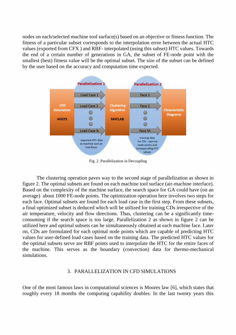
Fig. 2. Parallelization in Decoupling
The clustering operation paves way to the second stage of parallelization as shown in
figure 2. The optimal subsets are found on each machine tool surface (air-machine interface).
Based on the complexity of the machine surface, the search space for GA could have (on an
average) about 1000 FE-node points. The optimization operation here involves two steps for
each face. Optimal subsets are found for each load case in the first step. From these subsets,
a final optimized subset is deduced which will be utilized for training CDs irrespective of the
air temperature, velocity and flow directions. Thus, clustering can be a significantly time-
consuming if the search space is too large. Parallelization 2 as shown in figure 2 can be
utilized here and optimal subsets can be simultaneously obtained at each machine face. Later
on, CDs are formulated for each optimal node points which are capable of predicting HTC
values for user-defined load cases based on the training data. The predicted HTC values for
the optimal subsets serve are RBF points used to interpolate the HTC for the entire faces of
the machine. This serves as the boundary (convection) data for thermo-mechanical
simulations.
3. PARALLELIZATION IN CFD SIMULATIONS
One of the most famous laws in computational sciences is Moores law [6], which states that
roughly every 18 months the computing capability doubles. In the last twenty years this
observation switched from single-core capabilities to multi core systems. Nowadays, all major
CPUs contain at least two cores. Multi-core systems, with more than 12 cores, are also
available. From this point of view recent software packages have to support multi core
systems to retain their efficiency. Furthermore the near future also heads to Exascale
computing, refer to the investigation by Markidis et al [7].
Speaking of parallel architectures, in the sense of software as well as hardware, there
are two main categories. The so called shared memory systems belong to the first category.
The attribute shared refers to the memory of the processes running on a single system. Hence
every process might (but not have to) access the memory of another process. This makes
communication and data exchange efficient. For very tightly coupled algorithms this
approach is therefore advantageous. But it comes at the drawback that every process also
shares the connections between memory and CPU with the neighboring process. Hence
algorithms, which rely on a lot of memory per instruction are often bandwidth bound.
The other category involves the distributed systems. In this case every process runs on
its own system and has only direct access to the own memory and CPU. This architecture
makes the communication less efficient, but it does not suffer from the memory bandwidth.
Hence this approach is especially interesting for parallel approaches with only small couplings
and independent processes, refer to the literature survey by Tanenbaum et al [8].
The efficient parallel computation of the HTC for different load configurations requires
each simulation to be defined in a unique way. The design points (in ANSYS) are used to
identify each experiment and make them independent to each other. This structure allows the
simulations to be run concurrently. Furthermore, the access to the (heterogeneous) HPC
system with around 47000 processors allows each simulation to be run on distinct sets of
processors.
It is widely known that the runtime of CFD computations depend drastically on the
numerical and physical parameters. Incidentally, in the experiment under consideration,
variable runtimes were not seen. Very similar runtimes were obtained for every design point.
Hence, approximately the same resources could be reserved for every simulation without any
drawback.
Parallelization 1, as explained in section 2 involves parallel computation of CFD
simulations in ANSYS-CFX. A sufficiently complex CAD-geometry of a machine tool within
air medium needs to be chosen to effectively interpret the parallelization of decoupling
approach. The CAD model should be justifiable, considering the application of parallelization
in a moving machine component under varying environmental influences.
The major objective of CFD simulations in CFX is to provide simulation data (basically
HTCs with corresponding FE-coordinates) for each face under each combination of
environmental parameters such as ambient temperature, air velocity and air flow directions
(azimuth and elevation angles). HTCs are static and relatively smooth on any given flat
surface. They have a tendency to fluctuate strongly at edges between two surfaces. Therefore,
as long as each machine tool face (2D surfaces) is considered independently, the CDs are
expected to store and interpolate HTCs with sufficient accuracy, refer Naumann et al. [3].
Depending on the complexity and size of the FE-mesh used, the simulation duration can vary
from a few minutes to several hours.
All major FE tools, including ANSYS-CFX, provide at least an “internal” parallelization
of the FE discretization. The parallelization in ANSYS CFX utilizes the Single Program
Multiple Data (SPMD) concept. The model and mesh is decomposed into several partitions
that are executed as independent tasks that periodically exchange data for solution update.
Each process executes the same computations as in a serial run mode. In simple words, the
work is evenly distributed and load balanced. This widely used approach is extended for the
parallel computation of the HTCs for the CDs. Each simulation with a fixed tuple (Tair, v, az,
el), referring to the velocity, ambient temperature and flow directions - azimuth and elevation
respectively, computes the HTCs for this setting on all faces. In other words, the simulations
are independent for different combinations of environmental influences/parameters.
The independence among load cases facilitates every simulation to be run in parallel. The
software package ANSYS-CFX provides two features to accomplish the parallelization. First,
it allows the definition of design points. These points represent the physical parameters
velocity and ambient temperature. Second, it features an external python interface through
ANSYS/ACT. With this interface, the design point selection, simulation and extraction of
convection data on all desired faces afterwards, are automated without user interaction.
Both the above mentioned features are combined for parallelization. At first, an ANSYS-
CFX python script is prepared, which runs the simulation for the desired design point and
stores the HTC values for all desired faces. Afterwards, a shell script is prepared for the batch
system, which is parameterized with the design point. This script then runs ANSYS-CFX in
batch mode with the python script and the design point ID.
4. PARALLELIZATION IN CLUSTERING FE-NODES
4.1 Introduction to Clustering Algorithm
Clustering is the task of grouping a set of objects in such a way that objects in the same group,
called a cluster, are more similar (based on the objective) to each other than to those in other
groups. Formally, given a data set of ’m’ dimensions and ’n’ points, 𝐷 ∈ 𝑅{𝑛,𝑚} ={𝑑1, . . . , 𝑑𝑛}, clustering is the process of dividing the points up into ‘k’ groups (clusters) based
on a similarity measure. The search for a universal or more generic search algorithm led to
the discussion on GAs. The GA attempts to find a very good (or best) solution to the problem
by genetically breeding the population of individuals over a series of generations and
effectively overcome local minima based on Darwinian principle of reproduction and survival
of the fittest, analogous of naturally occurring genetic operations such as crossover and
mutation (refer to the works by John R Koza [9] and Koenig [10]).
Genetic Algorithm was introduced as a clustering technique and implemented
in decoupling approach in work by Glänzel et al. [5]. As discussed in the section 2, the purpose
of clustering in decoupling approach is to reduce the number of nodes and corresponding
HTC values used for training CDs. Maintaining accuracy in interpolation even after reduction
of nodes is very important. This is done by choosing optimal subsets of nodes with a fixed
size ‘m’ of node number values over each face of the machine, which will be used to build
an interpolation function, based on RBFs. The GA addresses the ‘Optimal Subset Problem’
(refer to the work by Unger et al. [11]) by minimizing the weighting function ‘f ’ as
min𝑆⊂𝑉
|𝑆|=𝑚
𝑓(𝑆) (1)
where V is the set of node numbers on a particular face, V = {1, 2 …N} which corresponds
with nodes 𝑥1, 𝑥2, . … 𝑥𝑁 of the finite element mesh and the simulated HTC values
𝑤1, 𝑤2, . … 𝑤𝑁 in these nodes. In the decoupling approach, the weighting function will
calculate the interpolation error which occurs when the ‘m’ nodes of ‘S’ are used to interpolate
the HTC values over an entire machine face, such that error measure in pointwise computed
form (2), f(S) becomes zero if m = N, and becomes greater than zero if m < N.
𝑓(𝑆) ≔ 𝑚𝑎𝑥𝑖=1…𝑁
|𝑓𝑠 (𝑥𝑖) − 𝑤𝑖| (2)
The major advantage of GA is that it can be used in those situations where the numerical or
mathematical models fail. GA, being an evolutionary algorithm, the progress can be viewed
with each iteration.
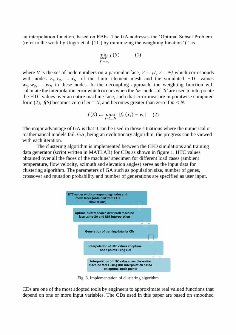
The clustering algorithm is implemented between the CFD simulations and training
data generator (script written in MATLAB) for CDs as shown in figure 1. HTC values
obtained over all the faces of the machine/ specimen for different load cases (ambient
temperature, flow velocity, azimuth and elevation angles) serve as the input data for
clustering algorithm. The parameters of GA such as population size, number of genes,
crossover and mutation probability and number of generations are specified as user input.
Fig. 3. Implementation of clustering algorithm
CDs are one of the most adopted tools by engineers to approximate real valued functions that
depend on one or more input variables. The CDs used in this paper are based on smoothed
grid regression technique suggested in the work by Priber [2]. It was later improved to high
dimensional CDs which were able to approximate thermo-elastic deformations in machine
tools. CDs are continuous maps of a set of input variables onto a single output variable. They
consist of a grid of support points along with kernel functions which describe the interpolation
in between, refer to the work by Putz et al. [12].
In decoupling approach, training data for CDs are developed using optimal node
points. Thus, each CD corresponds to a particular optimal node. HTC values are interpolated
over the optimal nodes based on the user defined load cases. Finally, HTC values are
interpolated again over the entire faces of the machine using HTC values on the optimal
nodes. Thus, the algorithm involves three interpolation processes at different stages of the
workflow. RBF interpolation is utilized initially to find the optimal subset and finally to
interpolate HTC over all the faces. CDs are used to interpolate the HTCs over optimal node
points.
Parallelization 2 basically attempts in running the GA operations simultaneously and
thereby finding the optimal node points on each prominent machine tool –air interfaces, which
are expected to contribute the most to the thermo-structural displacements on the machine
tool and thereby, TCP.
4.2 Static Load balancing for the parallelization of the GA operations
Parallelization 2 yields optimal FE-node points at selected machine faces. The training data
for CDs is formulated based on these optimal node points such that at each optimal node
point, environmental influences such as air flow temperature, velocity and directions of flow
(azimuth and elevation angles) are parameterized and mapped onto the corresponding HTC
values (𝛼). Thus, it would eliminate the need to consider position co-ordinates as input
variables in CDs. In the current implementation, air temperature, velocity, azimuth and
elevations angles of air flow corresponding to each optimal node point would serve as the
input parameters, refer [3]. Therefore, the main aim is to try and quantify the following
correlation:
(𝑇𝑎𝑖𝑟 , 𝑣, 𝑎𝑧, 𝑒𝑙 ) → 𝛼 (3)
The basis for the parallelization 2 (shown in figure 2) is the independence of clustering
operation among the machine tool faces. Every face has different optimal node selection, and
every selection is independent from the other faces. The evaluation costs of the fitness
function depend quadratically on the number of nodes. Hence the runtimes for every face vary
drastically, which leads to unbalanced parallelization and low efficiency.
Load balancing algorithms solve this issue. These algorithms use an estimate for the
runtimes and partition the tasks into several sub set. Depending on the constraints and fixed
or variable number of processors, these partitioning problems are sorted to different problem
classes. But all of them belong to the NP (nondeterministic polynomial time) problem class,
refer to work by Johnson [13]. Hence solutions are often only nearly optimal and the
algorithms are based on heuristics.
The static load balancing uses runtime estimates for every task and assigns the tasks to
the processors. These estimates are obtained by running a subset of all simulation parameters
and computing an approximation polynomial from their runtimes. Later on, runtimes are
extrapolated based on the remaining number of nodes. The aim is a short overall runtime with
the least number of processors as possible. The algorithm for a nearly optimal approximate
partitioning is similar to the first-fit decreasing algorithm, as mentioned in [14]. In this
algorithm every 'bin' represents a processor and faces are added into the bins. All faces in one
bin are computed sequentially. Originally the algorithm requires a fixed bin size, which would
correspond to the maximal runtime per core. But that size has to be minimized too and is not
known a priory. Hence the bin selection has to be changed from "fit-first" to "smallest work".
The algorithm starts with sorted faces with respect to their estimated work in
decreasing order. Afterwards the faces are assigned from highest to lowest work sequentially
to the bin with lowest work. Whereas the original first-fit algorithm requires a fixed bin size,
this strategy tries to keep the bin sizes minimal. The number of processors corresponds to the
number of bins, which is to be minimized too. That minimization can be approximated by
trying an increasing number of bins and stop, if the total estimated runtime does not decrease.
If the runtime, or the maximum work of the bins, is less than the runtime in the previous
iteration with a smaller number of bins, the number of bins is increased and the assignment
gets restarted. The implementation of static load balancing will be illustrated in the next
section where machine tool faces under investigation will be assigned to bins depending on
the runtime of clustering.
5. CASE STUDY- REDUCTION OF THE COMPUTATIONAL TIME WITH
(DISTRIBUTED) PARALLELIZATION
5.1 Simulation Model
The basic idea or motive behind parallelization of decoupling simulation approach is to reduce
the computation time involved in two processes:
i. CFD Simulations in ANSYS CFX
ii. Optimal subset search in MATLAB.
The extend to which this approach is effective can only be identified by performing the
operations on a sufficiently complex and justifiable simulation model. The geometry chosen
for this investigation is the machine tool- Auerbach ACW 630, a three-axis milling machine
of the Chemnitz University of Technology. The motive behind every scientific investigation
is to obtain results in close acceptance to real-life scenarios. The simulation model chosen for
this investigation involves the machine tool within an octagonal flow environment. Octagonal
faces facilitate a multitude of flow directions around the machine tool. However, for the
current case study, only one flow direction will be utilized with only ambient air temperature
and air velocities varying.
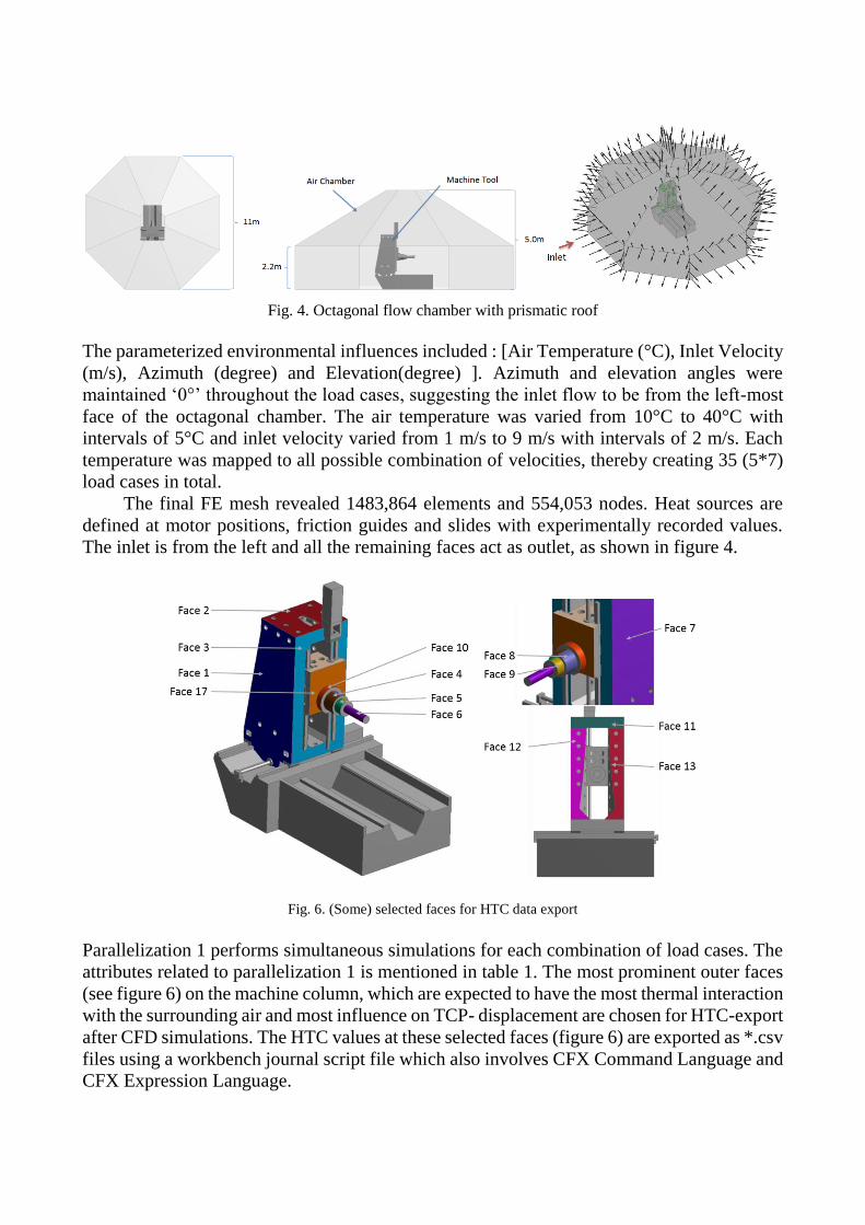
Fig. 4. Octagonal flow chamber with prismatic roof
The parameterized environmental influences included : [Air Temperature (°C), Inlet Velocity
(m/s), Azimuth (degree) and Elevation(degree) ]. Azimuth and elevation angles were
maintained ‘0°’ throughout the load cases, suggesting the inlet flow to be from the left-most
face of the octagonal chamber. The air temperature was varied from 10°C to 40°C with
intervals of 5°C and inlet velocity varied from 1 m/s to 9 m/s with intervals of 2 m/s. Each
temperature was mapped to all possible combination of velocities, thereby creating 35 (5*7)
load cases in total.
The final FE mesh revealed 1483,864 elements and 554,053 nodes. Heat sources are
defined at motor positions, friction guides and slides with experimentally recorded values.
The inlet is from the left and all the remaining faces act as outlet, as shown in figure 4.
Fig. 6. (Some) selected faces for HTC data export
Parallelization 1 performs simultaneous simulations for each combination of load cases. The
attributes related to parallelization 1 is mentioned in table 1. The most prominent outer faces
(see figure 6) on the machine column, which are expected to have the most thermal interaction
with the surrounding air and most influence on TCP- displacement are chosen for HTC-export
after CFD simulations. The HTC values at these selected faces (figure 6) are exported as *.csv
files using a workbench journal script file which also involves CFX Command Language and
CFX Expression Language.
Table 1. Attributes and procedure: Parallelization 1
Architecture Haswell
Manufacturer Intel
Memory upper bound 4069 MB
5.2 Comparison and quantification of reduction in runtime for simulation decoupling.
The previously described simulations are uniquely defined by the geometry and the surface
velocity. Hence each simulation is independent from the others and they can be run
simultaneously. From a technical point of view the simulations are controlled by the ANSYS
scripting engine, refer AnsysACT [15] and a job queue which manages the resources.
The figure 7 depicts the runtimes of the simulations for every experiment with blue
bars and the operational time for copy and wait in red and orange respectively. All jobs start
nearly immediately which is more of an exception. The organization and internal setup of
ANSYS require a copy of every simulation beforehand. However, the copying times are
negligible compared to the runtimes. Therefore, backing up the original model and running
every simulation on a backup does not lead to a significant time overhead.
Fig.7. Parallel runtime of the simulation together with the management operations for project file copy and
batch system wait times.
On the first sight at figure 7 a very strong variation in the simulation times can be observed
between 6000 seconds and 4500 seconds. This can have several reasons. One reason is the
heterogenous structure of HPC systems at ZIH/TU-Dresden (refer [16]).
The batch system, which manages the job queue, selects the nodes according to the usage
and therefore might select nodes with older CPUs. On the other hand every simulation runs
with another parameter set and the underlying numerical methods might be very sensitive to
these parameters too. Nevertheless with all simulations run in parallel, hence the total wall
clock time is below two hours. In contrast, a complete sequential simulation of all 35
experiments would have lasted more than 177914s ~ 50h. In other words the parallel
approach led to a good speedup about 31 with 35 cores.
5.3 Runtimes of statically balanced parallelization
Parallelization 2 presents a new set of challenges since the runtimes for each clustering
operation per machine face can vary drastically from each other. As stated in the load-
balancing algorithm, runtime estimates are required for the assignment. From an efficiency
point of view, faces with smallest runtime are selected along with a small number of medium
sized faces and their runtimes are measured. From these runtimes, the approximation
polynomial as shown in figure 8 can be obtained.
Fig.8. the runtimes for some faces and a quadratic polynomial fit. (cross denotes the faces used for
estimation, whereas the circles depict all runtimes.
The measured runtimes for some faces and the quadratic fitting polynomial is given in
figure 8. There were five faces used for runtime estimation. The corresponding quadratic
polynomial also estimated the runtimes for the other faces with acceptable precision.
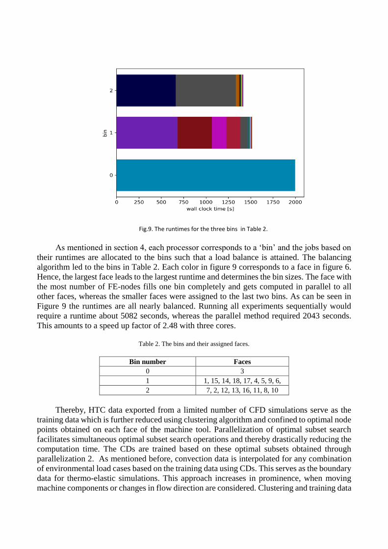
Fig.9. The runtimes for the three bins in Table 2.
As mentioned in section 4, each processor corresponds to a ‘bin’ and the jobs based on
their runtimes are allocated to the bins such that a load balance is attained. The balancing
algorithm led to the bins in Table 2. Each color in figure 9 corresponds to a face in figure 6.
Hence, the largest face leads to the largest runtime and determines the bin sizes. The face with
the most number of FE-nodes fills one bin completely and gets computed in parallel to all
other faces, whereas the smaller faces were assigned to the last two bins. As can be seen in
Figure 9 the runtimes are all nearly balanced. Running all experiments sequentially would
require a runtime about 5082 seconds, whereas the parallel method required 2043 seconds.
This amounts to a speed up factor of 2.48 with three cores.
Table 2. The bins and their assigned faces.
Bin number Faces
0 3
1 1, 15, 14, 18, 17, 4, 5, 9, 6,
2 7, 2, 12, 13, 16, 11, 8, 10
Thereby, HTC data exported from a limited number of CFD simulations serve as the
training data which is further reduced using clustering algorithm and confined to optimal node
points obtained on each face of the machine tool. Parallelization of optimal subset search
facilitates simultaneous optimal subset search operations and thereby drastically reducing the
computation time. The CDs are trained based on these optimal subsets obtained through
parallelization 2. As mentioned before, convection data is interpolated for any combination
of environmental load cases based on the training data using CDs. This serves as the boundary
data for thermo-elastic simulations. This approach increases in prominence, when moving
machine components or changes in flow direction are considered. Clustering and training data
generation in such scenarios would be extremely time-consuming if parallelization is not
utilized.
6. SUMMARY, CONCLUSION AND OUTLOOK
Decoupling of fluid simulations from thermo-mechanical simulations is of growing
significance in thermal-error prediction because of the complexities of the geometries and
dynamic behaviours of machine parts involved. For each variation in environmental
conditions around a machine tool, it is impractical to perform highly time-consuming CFD
simulations for boundary data in order to ascertain the corresponding thermal displacements.
Decoupling approach predicts convection data for thermo-mechanical simulations based on
trained characteristic diagrams. Clustering algorithm accelerates the training operation by
efficiently optimizing the training data. Holistically however, the decoupling approach needs
to be quickened up by multiple factors in order to be incorporated as a reliable thermal-error
prediction method.
This paper attempts to overcome the shortcomings of the decoupling approach in terms
of computation time. Parallel computation is incorporated in two stages, which leads to the
training of CDs. Firstly, CFD simulations in ANSYS CFX are run in parallel utilizing the
independence of load cases among each other and almost identical runtimes for each
simulation. On recent high performance clusters, every simulation can run in parallel, leading
to nearly optimal speed ups. With 35 cores a good speed up of about a factor of 31 was
obtained.
The second stage of parallelization, involves optimal subset search on each face of
the machine tool. The fitness function of GA represents the expensive function, which is
solved in parallel. Due to extremely different runtimes for each face, because of varying
number of FE-nodes ‘static load balancing’ algorithm is incorporated to efficiently place the
numerical experimental or jobs in ‘bins’ or processors. This optimal load balancing yields a
speed up of about 2.5 with three cores.
Both parallelization operations can be improved by an additional parallelization level.
The CFD simulations can fully employ the parallel advantages of distributed finite volume
methods. Using parallel linear algebra structures, the evaluation of fitness function can be
quickened up further. Both approaches require a sophisticated experimental organization on
the high performance clusters.
The future scope of work would include parallelization in decoupling for a dynamic
machine, where positions of the moving components should also be considered as input
parameters in CDs. The environmental influences could also be defined as functions of time
if the movement of machine components are pre-known. All possible flow directions should
be incorporated as well and evaluation times compared.
ACKNOWLEDGEMENTS
This research was supported by a German Research Foundation (DFG) grant within the Collaborative Research
Centers/Transregio 96, which is gratefully acknowledged.
REFERENCES
[1] J. GLAENZEL, S. IHLENFELDT, C. NAUMANN UND M. PUTZ. Efficient quantification of free and forced convection via
the decoupling of thermo-mechanical and thermo-fluidic simulations of machine tools. Journal of Machine Engineering,