59
Partial Differential Equations Paul Dawkins

Partial Differential Equations
Paul Dawkins

Differential Equations i
© 2018 Paul Dawkins http://tutorial.math.lamar.edu
Table of Contents Chapter 9 : Partial Differential Equations ............................................................................................................... 2
Section 9-1 : The Heat Equation ................................................................................................................................ 4 Section 9-2 : The Wave Equation ............................................................................................................................ 11 Section 9-3 : Terminology ....................................................................................................................................... 13 Section 9-4 : Separation of Variables ...................................................................................................................... 16 Section 9-5 : Solving the Heat Equation .................................................................................................................. 27 Section 9-6 : Heat Equation with Non-Zero Temperature Boundaries ................................................................... 40 Section 9-7 : Laplace's Equation .............................................................................................................................. 43 Section 9-8 : Vibrating String ................................................................................................................................... 54 Section 9-9 : Summary of Separation of Variables .................................................................................................. 57

Differential Equations 2
© 2018 Paul Dawkins http://tutorial.math.lamar.edu
Chapter 9 : Partial Differential Equations In this chapter we are going to take a very brief look at one of the more common methods for solving simple partial differential equations. The method we’ll be taking a look at is that of Separation of Variables. We need to make it very clear before we even start this chapter that we are going to be doing nothing more than barely scratching the surface of not only partial differential equations but also of the method of separation of variables. It would take several classes to cover most of the basic techniques for solving partial differential equations. The intent of this chapter is to do nothing more than to give you a feel for the subject and if you’d like to know more taking a class on partial differential equations should probably be your next step. Also note that in several sections we are going to be making heavy use of some of the results from the previous chapter. That in fact was the point of doing some of the examples that we did there. Having done them will, in some cases, significantly reduce the amount of work required in some of the examples we’ll be working in this chapter. When we do make use of a previous result we will make it very clear where the result is coming from. Here is a brief listing of the topics covered in this chapter. The Heat Equation – In this section we will do a partial derivation of the heat equation that can be solved to give the temperature in a one dimensional bar of length L. In addition, we give several possible boundary conditions that can be used in this situation. We also define the Laplacian in this section and give a version of the heat equation for two or three dimensional situations. The Wave Equation – In this section we do a partial derivation of the wave equation which can be used to find the one dimensional displacement of a vibrating string. In addition, we also give the two and three dimensional version of the wave equation. Terminology – In this section we take a quick look at some of the terminology we will be using in the rest of this chapter. In particular we will define a linear operator, a linear partial differential equation and a homogeneous partial differential equation. We also give a quick reminder of the Principle of Superposition. Separation of Variables – In this section show how the method of Separation of Variables can be applied to a partial differential equation to reduce the partial differential equation down to two ordinary differential equations. We apply the method to several partial differential equations. We do not, however, go any farther in the solution process for the partial differential equations. That will be done in later sections. The point of this section is only to illustrate how the method works. Solving the Heat Equation – In this section we go through the complete separation of variables process, including solving the two ordinary differential equations the process generates. We will do this by solving the heat equation with three different sets of boundary conditions. Included is an example solving the heat equation on a bar of length L but instead on a thin circular ring.

Differential Equations 3
© 2018 Paul Dawkins http://tutorial.math.lamar.edu
Heat Equation with Non-Zero Temperature Boundaries – In this section we take a quick look at solving the heat equation in which the boundary conditions are fixed, non-zero temperature. Note that this is in contrast to the previous section when we generally required the boundary conditions to be both fixed and zero. Laplace’s Equation – In this section we discuss solving Laplace’s equation. As we will see this is exactly the equation we would need to solve if we were looking to find the equilibrium solution (i.e. time independent) for the two dimensional heat equation with no sources. We will also convert Laplace’s equation to polar coordinates and solve it on a disk of radius a. Vibrating String – In this section we solve the one dimensional wave equation to get the displacement of a vibrating string. Summary of Separation of Variables – In this final section we give a quick summary of the method of separation of variables for solving partial differential equations.

Differential Equations 4
© 2018 Paul Dawkins http://tutorial.math.lamar.edu
Section 9-1 : The Heat Equation Before we get into actually solving partial differential equations and before we even start discussing the method of separation of variables we want to spend a little bit of time talking about the two main partial differential equations that we’ll be solving later on in the chapter. We’ll look at the first one in this section and the second one in the next section. The first partial differential equation that we’ll be looking at once we get started with solving will be the heat equation, which governs the temperature distribution in an object. We are going to give several forms of the heat equation for reference purposes, but we will only be really solving one of them. We will start out by considering the temperature in a 1-D bar of length L. What this means is that we are going to assume that the bar starts off at 0x = and ends when we reach x L= . We are also going to so assume that at any location, x the temperature will be constant at every point in the cross section at that x. In other words, temperature will only vary in x and we can hence consider the bar to be a 1-D bar. Note that with this assumption the actual shape of the cross section (i.e. circular, rectangular, etc.) doesn’t matter. Note that the 1-D assumption is actually not all that bad of an assumption as it might seem at first glance. If we assume that the lateral surface of the bar is perfectly insulated (i.e. no heat can flow through the lateral surface) then the only way heat can enter or leave the bar as at either end. This means that heat can only flow from left to right or right to left and thus creating a 1-D temperature distribution. The assumption of the lateral surfaces being perfectly insulated is of course impossible, but it is possible to put enough insulation on the lateral surfaces that there will be very little heat flow through them and so, at least for a time, we can consider the lateral surfaces to be perfectly insulated. Okay, let’s now get some definitions out of the way before we write down the first form of the heat equation.
( )( )( )( )( )
, Temperature at any point and any time
Specific Heat
Mass Density
, Heat Flux
, Heat energy generated per unit volume per unit time
u x t x t
c x
x
x t
Q x t
ρ
ϕ
=
=
=
=
=
We should probably make a couple of comments about some of these quantities before proceeding. The specific heat, ( ) 0c x > , of a material is the amount of heat energy that it takes to raise one unit of mass of the material by one unit of temperature. As indicated we are going to assume, at least initially, that the specific heat may not be uniform throughout the bar. Note as well that in practice the specific heat depends upon the temperature. However, this will generally only be an issue for large temperature differences (which in turn depends on the material the bar is made out of) and so we’re

Differential Equations 5
© 2018 Paul Dawkins http://tutorial.math.lamar.edu
going to assume for the purposes of this discussion that the temperature differences are not large enough to affect our solution. The mass density, ( )xρ , is the mass per unit volume of the material. As with the specific heat we’re going to initially assume that the mass density may not be uniform throughout the bar. The heat flux, ( ),x tϕ , is the amount of thermal energy that flows to the right per unit surface area per
unit time. The “flows to the right” bit simply tells us that if ( ), 0x tϕ > for some x and t then the heat is
flowing to the right at that point and time. Likewise, if ( ), 0x tϕ < then the heat will be flowing to the left at that point and time. The final quantity we defined above is ( ),Q x t and this is used to represent any external sources or
sinks (i.e. heat energy taken out of the system) of heat energy. If ( ), 0Q x t > then heat energy is being
added to the system at that location and time and if ( ), 0Q x t < then heat energy is being removed from the system at that location and time. With these quantities the heat equation is,
( ) ( ) ( ),uc x x Q x tt x
ϕρ ∂ ∂= − +
∂ ∂ (1)
While this is a nice form of the heat equation it is not actually something we can solve. In this form there are two unknown functions, u and ϕ , and so we need to get rid of one of them. With Fourier’s law we can easily remove the heat flux from this equation. Fourier’s law states that,
( ) ( )0, ux t K xx
ϕ ∂= −
∂
where ( )0 0K x > is the thermal conductivity of the material and measures the ability of a given
material to conduct heat. The better a material can conduct heat the larger ( )0K x will be. As noted the thermal conductivity can vary with the location in the bar. Also, much like the specific heat the thermal conductivity can vary with temperature, but we will assume that the total temperature change is not so great that this will be an issue and so we will assume for the purposes here that the thermal conductivity will not vary with temperature. Fourier’s law does a very good job of modeling what we know to be true about heat flow. First, we
know that if the temperature in a region is constant, i.e. 0ux∂
=∂
, then there is no heat flow.
Next, we know that if there is a temperature difference in a region we know the heat will flow from the hot portion to the cold portion of the region. For example, if it is hotter to the right then we know that

Differential Equations 6
© 2018 Paul Dawkins http://tutorial.math.lamar.edu
the heat should flow to the left. When it is hotter to the right then we also know that 0ux∂
>∂
(i.e. the
temperature increases as we move to the right) and so we’ll have 0ϕ < and so the heat will flow to the
left as it should. Likewise, if 0ux∂
<∂
(i.e. it is hotter to the left) then we’ll have 0ϕ > and heat will flow
to the right as it should.
Finally, the greater the temperature difference in a region (i.e. the larger ux∂∂
is) then the greater the
heat flow. So, if we plug Fourier’s law into (1), we get the following form of the heat equation,
( ) ( ) ( ) ( )0 ,u uc x x K x Q x tt x x
ρ ∂ ∂ ∂ = + ∂ ∂ ∂ (2)
Note that we factored the minus sign out of the derivative to cancel against the minus sign that was already there. We cannot however, factor the thermal conductivity out of the derivative since it is a function of x and the derivative is with respect to x. Solving (2) is quite difficult due to the non uniform nature of the thermal properties and the mass density. So, let’s now assume that these properties are all constant, i.e., ( ) ( ) ( )0 0c x c x K x Kρ ρ= = = where c, ρ and 0K are now all fixed quantities. In this case we generally say that the material in the bar is uniform. Under these assumptions the heat equation becomes,
( )2
0 2 ,u uc K Q x tt x
ρ ∂ ∂= +
∂ ∂ (3)
For a final simplification to the heat equation let’s divide both sides by cρ and define the thermal diffusivity to be,
0Kkcρ
=
The heat equation is then,
( )2
2
,Q x tu ukt x cρ
∂ ∂= +
∂ ∂ (4)
To most people this is what they mean when they talk about the heat equation and in fact it will be the equation that we’ll be solving. Well, actually we’ll be solving (4) with no external sources, i.e.( ), 0Q x t = , but we’ll be considering this form when we start discussing separation of variables in a
couple of sections. We’ll only drop the sources term when we actually start solving the heat equation. Now that we’ve got the 1-D heat equation taken care of we need to move into the initial and boundary conditions we’ll also need in order to solve the problem. If you go back to any of our solutions of

Differential Equations 7
© 2018 Paul Dawkins http://tutorial.math.lamar.edu
ordinary differential equations that we’ve done in previous sections you can see that the number of conditions required always matched the highest order of the derivative in the equation. In partial differential equations the same idea holds except now we have to pay attention to the variable we’re differentiating with respect to as well. So, for the heat equation we’ve got a first order time derivative and so we’ll need one initial condition and a second order spatial derivative and so we’ll need two boundary conditions. The initial condition that we’ll use here is,
( ) ( ),0u x f x= and we don’t really need to say much about it here other than to note that this just tells us what the initial temperature distribution in the bar is. The boundary conditions will tell us something about what the temperature and/or heat flow is doing at the boundaries of the bar. There are four of them that are fairly common boundary conditions. The first type of boundary conditions that we can have would be the prescribed temperature boundary conditions, also called Dirichlet conditions. The prescribed temperature boundary conditions are, ( ) ( ) ( ) ( )1 20, ,u t g t u L t g t= = The next type of boundary conditions are prescribed heat flux, also called Neumann conditions. Using Fourier’s law these can be written as,
( ) ( ) ( ) ( ) ( ) ( )0 1 0 20 0, ,u uK t t K L L t tx x
ϕ ϕ∂ ∂− = − =
∂ ∂
If either of the boundaries are perfectly insulated, i.e. there is no heat flow out of them then these boundary conditions reduce to,
( ) ( )0, 0 , 0u ut L tx x∂ ∂
= =∂ ∂
and note that we will often just call these particular boundary conditions insulated boundaries and drop the “perfectly” part. The third type of boundary conditions use Newton’s law of cooling and are sometimes called Robins conditions. These are usually used when the bar is in a moving fluid and note we can consider air to be a fluid for this purpose. Here are the equations for this kind of boundary condition.
( ) ( ) ( ) ( ) ( ) ( ) ( ) ( )0 1 0 20 0, 0, , ,u uK t H u t g t K L L t H u L t g tx x∂ ∂
− = − − − = − ∂ ∂
where H is a positive quantity that is experimentally determined and ( )1g t and ( )2g t give the temperature of the surrounding fluid at the respective boundaries. Note that the two conditions do vary slightly depending on which boundary we are at. At 0x = we have a minus sign on the right side while we don’t at x L= . To see why this is let’s first assume that at
0x = we have ( ) ( )10,u t g t> . In other words, the bar is hotter than the surrounding fluid and so at

Differential Equations 8
© 2018 Paul Dawkins http://tutorial.math.lamar.edu
0x = the heat flow (as given by the left side of the equation) must be to the left, or negative since the heat will flow from the hotter bar into the cooler surrounding liquid. If the heat flow is negative then we need to have a minus sign on the right side of the equation to make sure that it has the proper sign. If the bar is cooler than the surrounding fluid at 0x = , i.e. ( ) ( )10,u t g t< we can make a similar argument to justify the minus sign. We’ll leave it to you to verify this. If we now look at the other end, x L= , and again assume that the bar is hotter than the surrounding fluid or, ( ) ( )2,u L t g t> . In this case the heat flow must be to the right, or be positive, and so in this case we can’t have a minus sign. Finally, we’ll again leave it to you to verify that we can’t have the minus sign at x L= is the bar is cooler than the surrounding fluid as well. Note that we are not actually going to be looking at any of these kinds of boundary conditions here. These types of boundary conditions tend to lead to boundary value problems such as Example 5 in the Eigenvalues and Eigenfunctions section of the previous chapter. As we saw in that example it is often very difficult to get our hands on the eigenvalues and as we’ll eventually see we will need them. It is important to note at this point that we can also mix and match these boundary conditions so to speak. There is nothing wrong with having a prescribed temperature at one boundary and a prescribed flux at the other boundary for example so don’t always expect the same boundary condition to show up at both ends. This warning is more important that it might seem at this point because once we get into solving the heat equation we are going to have the same kind of condition on each end to simplify the problem somewhat. The final type of boundary conditions that we’ll need here are periodic boundary conditions. Periodic boundary conditions are,
( ) ( ) ( ) ( ), , , ,u uu L t u L t L t L tx x∂ ∂
− = − =∂ ∂
Note that for these kinds of boundary conditions the left boundary tends to be x L= − instead of 0x = as we were using in the previous types of boundary conditions. The periodic boundary conditions will arise very naturally from a couple of particular geometries that we’ll be looking at down the road. We will now close out this section with a quick look at the 2-D and 3-D version of the heat equation. However, before we jump into that we need to introduce a little bit of notation first. The del operator is defined to be,
i j i j kx y x y k∂ ∂ ∂ ∂ ∂
∇ = + ∇ = + +∂ ∂ ∂ ∂ ∂
depending on whether we are in 2 or 3 dimensions. Think of the del operator as a function that takes functions as arguments (instead of numbers as we’re used to). Whatever function we “plug” into the operator gets put into the partial derivatives. So, for example in 3-D we would have,

Differential Equations 9
© 2018 Paul Dawkins http://tutorial.math.lamar.edu
f f ff i j kx y k∂ ∂ ∂
∇ = + +∂ ∂ ∂
This of course is also the gradient of the function ( ), ,f x y z . The del operator also allows us to quickly write down the divergence of a function. So, again using 3-D as an example the divergence of ( ), ,f x y z can be written as the dot product of the del operator and the function. Or,
f f ffx y k∂ ∂ ∂
∇ = + +∂ ∂ ∂
Finally, we will also see the following show up in our work,
( )2 2 2
2 2 2
f f f f f ffx x y y z k x y z
∂ ∂ ∂ ∂ ∂ ∂ ∂ ∂ ∂ ∇ ∇ = + + = + + ∂ ∂ ∂ ∂ ∂ ∂ ∂ ∂ ∂
This is usually denoted as,
2 2 2
22 2 2
f f ffx y z
∂ ∂ ∂∇ = + +
∂ ∂ ∂
and is called the Laplacian. The 2-D version of course simply doesn’t have the third term. Okay, we can now look into the 2-D and 3-D version of the heat equation and where ever the del operator and or Laplacian appears assume that it is the appropriate dimensional version. The higher dimensional version of (1) is,
uc Qt
ρ ϕ∂= −∇ +
∂ (5)
and note that the specific heat, c, and mass density, ρ , are may not be uniform and so may be functions of the spatial variables. Likewise, the external sources term, Q, may also be a function of both the spatial variables and time. Next, the higher dimensional version of Fourier’s law is, 0K uϕ = − ∇ where the thermal conductivity, 0K , is again assumed to be a function of the spatial variables. If we plug this into (5) we get the heat equation for a non uniform bar (i.e. the thermal properties may be functions of the spatial variables) with external sources/sinks,
( )0uc K u Qt
ρ ∂= ∇ ∇ +
∂ (6)
If we now assume that the specific heat, mass density and thermal conductivity are constant (i.e. the bar is uniform) the heat equation becomes,
2u Qk ut cp
∂= ∇ +
∂ (7)

Differential Equations 10
© 2018 Paul Dawkins http://tutorial.math.lamar.edu
where we divided both sides by cρ to get the thermal diffusivity, k in front of the Laplacian. The initial condition for the 2-D or 3-D heat equation is, ( ) ( ) ( ) ( ), , , or , , , , ,u x y t f x y u x y z t f x y z= = depending upon the dimension we’re in. The prescribed temperature boundary condition becomes, ( ) ( ) ( ) ( ), , , , or , , , , , ,u x y t T x y t u x y z t T x y z t= =
where ( ),x y or ( ), ,x y z , depending upon the dimension we’re in, will range over the portion of the boundary in which we are prescribing the temperature. The prescribed heat flux condition becomes, ( )0K u n tϕ− ∇ =
where the left side is only being evaluated at points along the boundary and n is the outward unit normal on the surface. Newton’s law of cooling will become, ( )0 BK u n H u u− ∇ = −
where H is a positive quantity that is experimentally determine, Bu is the temperature of the fluid at the boundary and again it is assumed that this is only being evaluated at points along the boundary. We don’t have periodic boundary conditions here as they will only arise from specific 1-D geometries. We should probably also acknowledge at this point that we’ll not actually be solving (7) at any point, but we will be solving a special case of it in the Laplace’s Equation section.

Differential Equations 11
© 2018 Paul Dawkins http://tutorial.math.lamar.edu
Section 9-2 : The Wave Equation In this section we want to consider a vertical string of length L that has been tightly stretched between two points at 0x = and x L= . Because the string has been tightly stretched we can assume that the slope of the displaced string at any point is small. So just what does this do for us? Let’s consider a point x on the string in its equilibrium position, i.e. the location of the point at 0t = . As the string vibrates this point will be displaced both vertically and horizontally, however, if we assume that at any point the slope of the string is small then the horizontal displacement will be very small in relation to the vertical displacement. This means that we can now assume that at any point x on the string the displacement will be purely vertical. So, let’s call this displacement ( ),u x t . We are going to assume, at least initially, that the string is not uniform and so the mass density of the string, ( )xρ may be a function of x. Next, we are going to assume that the string is perfectly flexible. This means that the string will have no resistance to bending. This in turn tells us that the force exerted by the string at any point x on the endpoints will be tangential to the string itself. This force is called the tension in the string and its magnitude will be given by ( ),T x t . Finally, we will let ( ),Q x t represent the vertical component per unit mass of any force acting on the string. Provided we again assume that the slope of the string is small the vertical displacement of the string at any point is then given by,
( ) ( ) ( ) ( )2
2 , ,u ux T x t x Q x tt x x
ρ ρ∂ ∂ ∂ = + ∂ ∂ ∂ (1)
This is a very difficult partial differential equation to solve so we need to make some further simplifications. First, we’re now going to assume that the string is perfectly elastic. This means that the magnitude of the tension, ( ),T x t , will only depend upon how much the string stretches near x. Again, recalling that we’re assuming that the slope of the string at any point is small this means that the tension in the string will then very nearly be the same as the tension in the string in its equilibrium position. We can then assume that the tension is a constant value, ( ) 0,T x t T= . Further, in most cases the only external force that will act upon the string is gravity and if the string light enough the effects of gravity on the vertical displacement will be small and so will also assume that ( ), 0Q x t = . This leads to

Differential Equations 12
© 2018 Paul Dawkins http://tutorial.math.lamar.edu
2 2
02 2
u uTt x
ρ ∂ ∂=
∂ ∂
If we now divide by the mass density and define,
2 0Tcρ
=
we arrive at the 1-D wave equation,
2 2
22 2
u uct x
∂ ∂=
∂ ∂ (2)
In the previous section when we looked at the heat equation he had a number of boundary conditions however in this case we are only going to consider one type of boundary conditions. For the wave equation the only boundary condition we are going to consider will be that of prescribed location of the boundaries or, ( ) ( ) ( ) ( )1 20, ,u t h t u L t h t= = The initial conditions (and yes we meant more than one…) will also be a little different here from what we saw with the heat equation. Here we have a 2nd order time derivative and so we’ll also need two initial conditions. At any point we will specify both the initial displacement of the string as well as the initial velocity of the string. The initial conditions are then,
( ) ( ) ( ) ( ),0 ,0uu x f x x g xt
∂= =
∂
For the sake of completeness we’ll close out this section with the 2-D and 3-D version of the wave equation. We’ll not actually be solving this at any point, but since we gave the higher dimensional version of the heat equation (in which we will solve a special case) we’ll give this as well. The 2-D and 3-D version of the wave equation is,
2
2 22
u c ut
∂= ∇
∂
where 2∇ is the Laplacian.
Differential Equations 13
© 2018 Paul Dawkins http://tutorial.math.lamar.edu
Section 9-3 : Terminology We’ve got one more section that we need to take care of before we actually start solving partial differential equations. This will be a fairly short section that will cover some of the basic terminology that we’ll need in the next section as we introduce the method of separation of variables. Let’s start off with the idea of an operator. An operator is really just a function that takes a function as an argument instead of numbers as we’re used to dealing with in functions. You already know of a couple of operators even if you didn’t know that they were operators. Here are some examples of operators.
b
a
dL L dx L dx Ldx t
∂= = = =
∂∫ ∫
Or, if we plug in a function, say ( )u x , into each of these we get,
( ) ( ) ( ) ( ) ( ) ( )b
a
du uL u L u u x dx L u u x dx L udx t
∂= = = =
∂∫ ∫
These are all fairly simple examples of operators but the derivative and integral are operators. A more complicated operator would be the heat operator. We get the heat operator from a slight rewrite of the heat equation without sources. The heat operator is,
2
2L kt x∂ ∂
= −∂ ∂
Now, what we really want to define here is not an operator but instead a linear operator. A linear operator is any operator that satisfies,
( ) ( ) ( )1 1 2 2 1 1 2 2L c u c u c L u c L u+ = + The heat operator is an example of a linear operator and this is easy enough to show using the basic properties of the partial derivative so let’s do that.
( ) ( ) ( )
( ) ( ) ( ) ( )
2
1 1 2 2 1 1 2 2 1 1 2 22
2 2
1 1 2 2 1 1 2 22 2
2 21 2 1 2
1 2 1 22 2
2 21 1 2 2
1 1 2 22 2
2 21 1 2 2
1 22
L c u c u c u c u k c u c ut x
c u c u k c u c ut t x x
u u u uc c k c ct t x x
u u u uc kc c kct x t xu u u uc k c kt x t
∂ ∂+ = + − +
∂ ∂ ∂ ∂ ∂ ∂
= + − + ∂ ∂ ∂ ∂ ∂ ∂ ∂ ∂
= + − + ∂ ∂ ∂ ∂ ∂ ∂ ∂ ∂
= − + −∂ ∂ ∂ ∂ ∂ ∂ ∂ ∂
= − + − ∂ ∂ ∂ ( ) ( )
2
1 1 2 2
x
c L u c L u
∂
= +
Differential Equations 14
© 2018 Paul Dawkins http://tutorial.math.lamar.edu
You might want to verify for yourself that the derivative and integral operators we gave above are also linear operators. In fact, in the process of showing that the heat operator is a linear operator we actually showed as well that the first order and second order partial derivative operators are also linear. The next term we need to define is a linear equation. A linear equation is an equation in the form,
( )L u f= (1) where L is a linear operator and f is a known function. Here are some examples of linear partial differential equations.
( )
( )
2
2
2 22
2 2
2 2 22
2 2 2
2 3
2 3
,
0
4 8 ,
Q x tu ukt x cu uc
t xu u u u
x y zu u u u g x tt t x
ρ∂ ∂
= +∂ ∂
∂ ∂=
∂ ∂∂ ∂ ∂
+ + = ∇ =∂ ∂ ∂
∂ ∂ ∂− = + −
∂ ∂ ∂
The first two from this list are of course the heat equation and the wave equation. The third uses the Laplacian and is usually called Laplace’s Equation. We’ll actually be solving the 2-D version of Laplace’s Equation in a few sections. The fourth equation was just made up to give a more complicated example.
Notice as well with the heat equation and the fourth example above that the presence of the ( ),Q x t
and ( ),g x t do not prevent these from being linear equations. The main issue that allows these to be
linear equations is the fact that the operator in each is linear. Now just to be complete here are a couple of examples of nonlinear partial differential equations.
( )
22
2
2
2 ,
u uk ut x
u u u u f x tt x t
∂ ∂= +
∂ ∂∂ ∂ ∂
− = +∂ ∂ ∂
We’ll leave it to you to verify that the operators in each of these are not linear however the problem term in the first is the 2u while in the second the product of the two derivatives is the problem term. Now, if we go back to (1) and suppose that 0f = then we arrive at,
( ) 0L u = (2) We call this a linear homogeneous equation (recall that L is a linear operator).

Differential Equations 15
© 2018 Paul Dawkins http://tutorial.math.lamar.edu
Notice that 0u = will always be a solution to a linear homogeneous equation (go back to what it means
to be linear and use 1 2 0c c= = with any two solutions and this is easy to verify). We call 0u = the trivial solution. In fact, this is also a really nice way of determining if an equation is homogeneous. If L
is a linear operator and we plug in 0u = into the equation and we get ( ) 0L u = then we will know that the operator is homogeneous. We can also extend the ideas of linearity and homogeneous to boundary conditions. If we go back to the various boundary conditions we discussed for the heat equation for example we can also classify them as linear and/or homogeneous. The prescribed temperature boundary conditions,
( ) ( ) ( ) ( )1 20, ,u t g t u L t g t= =
are linear and will only be homogenous if ( )1 0g t = and ( )2 0g t = . The prescribed heat flux boundary conditions,
( ) ( ) ( ) ( ) ( ) ( )0 1 0 20 0, ,u uK t t K L L t tx x
ϕ ϕ∂ ∂− = − =
∂ ∂
are linear and will again only be homogeneous if ( )1 0tϕ = and ( )2 0tϕ = .
Next, the boundary conditions from Newton’s law of cooling,
( ) ( ) ( ) ( ) ( ) ( ) ( ) ( )0 1 0 20 0, 0, , ,u uK t H u t g t K L L t H u L t g tx x∂ ∂
− = − − − = − ∂ ∂
are again linear and will only be homogenous if ( )1 0g t = and ( )2 0g t = . The final set of boundary conditions that we looked at were the periodic boundary conditions,
( ) ( ) ( ) ( ), , , ,u uu L t u L t L t L tx x∂ ∂
− = − =∂ ∂
and these are both linear and homogeneous. The final topic in this section is not really terminology but is a restatement of a fact that we’ve seen several times in these notes already. Principle of Superposition
If 1u and 2u are solutions to a linear homogeneous equation then so is 1 1 2 2c u c u+ for any values of
1c and 2c . Now, as stated earlier we’ve seen this several times this semester but we didn’t really do much with it. However, this is going to be a key idea when we actually get around to solving partial differential equations. Without this fact we would not be able to solve all but the most basic of partial differential equations.

Differential Equations 16
© 2018 Paul Dawkins http://tutorial.math.lamar.edu
Section 9-4 : Separation of Variables Okay, it is finally time to at least start discussing one of the more common methods for solving basic partial differential equations. The method of Separation of Variables cannot always be used and even when it can be used it will not always be possible to get much past the first step in the method. However, it can be used to easily solve the 1-D heat equation with no sources, the 1-D wave equation, and the 2-D version of Laplace’s Equation, 2 0u∇ = . In order to use the method of separation of variables we must be working with a linear homogenous partial differential equations with linear homogeneous boundary conditions. At this point we’re not going to worry about the initial condition(s) because the solution that we initially get will rarely satisfy the initial condition(s). As we’ll see however there are ways to generate a solution that will satisfy initial condition(s) provided they meet some fairly simple requirements. The method of separation of variables relies upon the assumption that a function of the form,
( ) ( ) ( ),u x t x G tϕ= (1) will be a solution to a linear homogeneous partial differential equation in x and t. This is called a product solution and provided the boundary conditions are also linear and homogeneous this will also satisfy the boundary conditions. However, as noted above this will only rarely satisfy the initial condition, but that is something for us to worry about in the next section. Now, before we get started on some examples there is probably a question that we should ask at this point and that is : Why? Why did we choose this solution and how do we know that it will work? This seems like a very strange assumption to make. After all there really isn’t any reason to believe that a solution to a partial differential equation will in fact be a product of a function of only x’s and a function of only t’s. This seems more like a hope than a good assumption/guess. Unfortunately, the best answer is that we chose it because it will work. As we’ll see it works because it will reduce our partial differential equation down to two ordinary differential equations and provided we can solve those then we’re in business and the method will allow us to get a solution to the partial differential equations. So, let’s do a couple of examples to see how this method will reduce a partial differential equation down to two ordinary differential equations. Example 1 Use Separation of Variables on the following partial differential equation.
( ) ( ) ( ) ( )
2
2
,0 0, 0 , 0
u ukt x
u x f x u t u L t
∂ ∂=
∂ ∂= = =
Solution So, we have the heat equation with no sources, fixed temperature boundary conditions (that are also homogeneous) and an initial condition. The initial condition is only here because it belongs here, but we will be ignoring it until we get to the next section.

Differential Equations 17
© 2018 Paul Dawkins http://tutorial.math.lamar.edu
The method of separation of variables tells us to assume that the solution will take the form of the product,
( ) ( ) ( ),u x t x G tϕ= so all we really need to do here is plug this into the differential equation and see what we get.
( ) ( )( ) ( ) ( )( )
( ) ( )
2
2
2
2
x G t k x G tt x
dG dx k G tdt dx
ϕ ϕ
ϕϕ
∂ ∂=
∂ ∂
=
As shown above we can factor the ( )xϕ out of the time derivative and we can factor the ( )G t out
of the spatial derivative. Also notice that after we’ve factored these out we no longer have a partial
derivative left in the problem. In the time derivative we are now differentiating only ( )G t with respect to t and this is now an ordinary derivative. Likewise, in the spatial derivative we are now only
differentiating ( )xϕ with respect to x and so we again have an ordinary derivative. At this point it probably doesn’t seem like we’ve done much to simplify the problem. However, just the fact that we’ve gotten the partial derivatives down to ordinary derivatives is liable to be good thing even if it still looks like we’ve got a mess to deal with. Speaking of that apparent (and yes we said apparent) mess, is it really the mess that it looks like? The idea is to eventually get all the t’s on one side of the equation and all the x’s on the other side. In other words, we want to “separate the variables” and hence the name of the method. In this case
let’s notice that if we divide both sides by ( ) ( )x G tϕ we get what we want and we should point out
that it won’t always be as easy as just dividing by the product solution. So, dividing out gives us,
2 2
2 2
1 1 1 1dG d dG dkG dt dx kG dt dx
ϕ ϕϕ ϕ
= ⇒ =
Notice that we also divided both sides by k. This was done only for convenience down the road. It doesn’t have to be done and nicely enough if it turns out to be a bad idea we can always come back to this step and put it back on the right side. Likewise, if we don’t do it and it turns out to maybe not be such a bad thing we can always come back and divide it out. For the time being however, please accept our word that this was a good thing to do for this problem. We will discuss the reasoning for this after we’re done with this example. Now, while we said that this is what we wanted it still seems like we’ve got a mess. Notice however that the left side is a function of only t and the right side is a function only of x as we wanted. Also notice these two functions must be equal. Let’s think about this for a minute. How is it possible that a function of only t’s can be equal to a function of only x’s regardless of the choice of t and/or x that we have? This may seem like an impossibility until you realize that there is one way that this can be true. If both functions (i.e. both sides of the equation) were in fact constant and not only a constant, but the same constant then they can in fact be equal.

Differential Equations 18
© 2018 Paul Dawkins http://tutorial.math.lamar.edu
So, we must have,
2
2
1 1dG dkG dt dx
ϕ λϕ
= = −
where the λ− is called the separation constant and is arbitrary. The next question that we should now address is why the minus sign? Again, much like the dividing out the k above, the answer is because it will be convenient down the road to have chosen this. The minus sign doesn’t have to be there and in fact there are times when we don’t want it there. So how do we know it should be there or not? The answer to that is to proceed to the next step in the process (which we’ll see in the next section) and at that point we’ll know if would be convenient to have it or not and we can come back to this step and add it in or take it our depending what we chose to do here. Okay, let’s proceed with the process. The next step is to acknowledge that we can take the equation above and split it into the following two ordinary differential equations.
2
2
dG dk Gdt dx
ϕλ λϕ= − = −
Both of these are very simple differential equations, however because we don’t know what λ is we actually can’t solve the spatial one yet. The time equation however could be solved at this point if we wanted to, although that won’t always be the case. At this point we don’t want to actually think about solving either of these yet however. The last step in the process that we’ll be doing in this section is to also make sure that our product
solution, ( ) ( ) ( ),u x t x G tϕ= , satisfies the boundary conditions so let’s plug it into both of those.
( ) ( ) ( ) ( ) ( ) ( )0, 0 0 , 0u t G t u L t L G tϕ ϕ= = = =
Let’s consider the first one for a second. We have two options here. Either ( )0 0ϕ = or ( ) 0G t = for
every t. However, if we have ( ) 0G t = for every t then we’ll also have ( ), 0u x t = , i.e. the trivial solution, and as we discussed in the previous section this is definitely a solution to any linear homogeneous equation we would really like a non-trivial solution.
Therefore, we will assume that in fact we must have ( )0 0ϕ = . Likewise, from the second boundary
condition we will get ( ) 0Lϕ = to avoid the trivial solution. Note as well that we were only able to reduce the boundary conditions down like this because they were homogeneous. Had they not been homogeneous we could not have done this. So, after applying separation of variables to the given partial differential equation we arrive at a 1st
order differential equation that we’ll need to solve for ( )G t and a 2nd order boundary value problem
Differential Equations 19
© 2018 Paul Dawkins http://tutorial.math.lamar.edu
that we’ll need to solve for ( )xϕ . The point of this section however is just to get to this point and we’ll hold off solving these until the next section. Let’s summarize everything up that we’ve determined here.
( ) ( )
2
2 0
0 0 0
dG dk Gdt dx
L
ϕλ λϕ
ϕ ϕ
= − + =
= =
and note that we don’t have a condition for the time differential equation and is not a problem. Also note that we rewrote the second one a little.
Okay, so just what have we learned here? By using separation of variables we were able to reduce our linear homogeneous partial differential equation with linear homogeneous boundary conditions down
to an ordinary differential equation for one of the functions in our product solution (1), ( )G t in this
case, and a boundary value problem that we can solve for the other function, ( )xϕ in this case. Note as well that the boundary value problem is in fact an eigenvalue/eigenfunction problem. When we solve the boundary value problem we will be identifying the eigenvalues, λ , that will generate non-trivial solutions to their corresponding eigenfunctions. Again, we’ll look into this more in the next section. At this point all we want to do is identify the two ordinary differential equations that we need to solve to get a solution. Before we do a couple of other examples we should take a second to address the fact that we made two very arbitrary seeming decisions in the above work. We divided both sides of the equation by k at one point and chose to use λ− instead of λ as the separation constant. Both of these decisions were made to simplify the solution to the boundary value problem we got from our work. The addition of the k in the boundary value problem would just have complicated the solution process with another letter we’d have to keep track of so we moved it into the time problem where it won’t cause as many problems in the solution process. Likewise, we chose λ− because we’ve already solved that particular boundary value problem (albeit with a specific L, but the work will be nearly identical) when we first looked at finding eigenvalues and eigenfunctions. This by the way was the reason we rewrote the boundary value problem to make it a little clearer that we have in fact solved this one already. We can now at least partially answer the question of how do we know to make these decisions. We wait until we get the ordinary differential equations and then look at them and decide of moving things like the k or which separation constant to use based on how it will affect the solution of the ordinary differential equations. There is also, of course, a fair amount of experience that comes into play at this stage. The more experience you have in solving these the easier it often is to make these decisions. Again, we need to make clear here that we’re not going to go any farther in this section than getting things down to the two ordinary differential equations. Of course, we will need to solve them in order to get a solution to the partial differential equation but that is the topic of the remaining sections in this chapter. All we’ll say about it here is that we will need to first solve the boundary value problem, which

Differential Equations 20
© 2018 Paul Dawkins http://tutorial.math.lamar.edu
will tell us what λ must be and then we can solve the other differential equation. Once that is done we can then turn our attention to the initial condition. Okay, we need to work a couple of other examples and these will go a lot quicker because we won’t need to put in all the explanations. After the first example this process always seems like a very long process but it really isn’t. It just looked that way because of all the explanation that we had to put into it. So, let’s start off with a couple of more examples with the heat equation using different boundary conditions. Example 2 Use Separation of Variables on the following partial differential equation.
( ) ( ) ( ) ( )
2
2
,0 0, 0 , 0
u ukt x
u uu x f x t L tx x
∂ ∂=
∂ ∂∂ ∂
= = =∂ ∂
Solution In this case we’re looking at the heat equation with no sources and perfectly insulated boundaries. So, we’ll start off by again assuming that our product solution will have the form,
( ) ( ) ( ),u x t x G tϕ= and because the differential equation itself hasn’t changed here we will get the same result from plugging this in as we did in the previous example so the two ordinary differential equations that we’ll need to solve are,
2
2
dG dk Gdt dx
ϕλ λϕ= − = −
Now, the point of this example was really to deal with the boundary conditions so let’s plug the product solution into them to get,
( ) ( )( ) ( ) ( ) ( )( ) ( )
( ) ( ) ( ) ( )
0, 0 , 0
0 0 0
G t x G t xt L t
x xd dG t G t Ldx dx
ϕ ϕ
ϕ ϕ
∂ ∂= =
∂ ∂
= =
Now, just as with the first example if we want to avoid the trivial solution and so we can’t have
( ) 0G t = for every t and so we must have,
( ) ( )0 0 0d d Ldx dxϕ ϕ
= =
Here is a summary of what we get by applying separation of variables to this problem.

Differential Equations 21
© 2018 Paul Dawkins http://tutorial.math.lamar.edu
( ) ( )
2
2 0
0 0 0
dG dk Gdt dx
d d Ldx dx
ϕλ λϕ
ϕ ϕ
= − + =
= =
Next, let’s see what we get if use periodic boundary conditions with the heat equation. Example 3 Use Separation of Variables on the following partial differential equation.
( ) ( ) ( ) ( ) ( ) ( )
2
2
,0 , , , ,
u ukt x
u uu x f x u L t u L t L t L tx x
∂ ∂=
∂ ∂∂ ∂
= − = − =∂ ∂
Solution First note that these boundary conditions really are homogeneous boundary conditions. If we rewrite them as,
( ) ( ) ( ) ( ), , 0 , , 0u uu L t u L t L t L tx x∂ ∂
− − = − − =∂ ∂
it’s a little easier to see. Now, again we’ve done this partial differential equation so we’ll start off with,
( ) ( ) ( ),u x t x G tϕ= and the two ordinary differential equations that we’ll need to solve are,
2
2
dG dk Gdt dx
ϕλ λϕ= − = −
Plugging the product solution into the rewritten boundary conditions gives,
( ) ( ) ( ) ( ) ( ) ( ) ( )
( ) ( ) ( ) ( ) ( ) ( ) ( )
0
0
G t L G t L G t L L
d d d dG t L G t L G t L Ldx dx dx dx
ϕ ϕ ϕ ϕ
ϕ ϕ ϕ ϕ
− − = − − = − − = − − =
and we can see that we’ll only get non-trivial solution if,
( ) ( ) ( ) ( )
( ) ( ) ( ) ( )
0 0d dL L L Ldx dx
d dL L L Ldx dx
ϕ ϕϕ ϕ
ϕ ϕϕ ϕ
− − = − − =
− = − =
So, here is what we get by applying separation of variables to this problem.
( ) ( ) ( ) ( )
2
2 0dG dk Gdt dx
d dL L L Ldx dx
ϕλ λϕ
ϕ ϕϕ ϕ
= − + =
− = − =

Differential Equations 22
© 2018 Paul Dawkins http://tutorial.math.lamar.edu
Let’s now take a look at what we get by applying separation of variables to the wave equation with fixed boundaries. Example 4 Use Separation of Variables on the following partial differential equation.
( ) ( ) ( ) ( )
( ) ( )
2 22
2 2
,0 ,0
0, 0 , 0
u uct x
uu x f x x g xt
u t u L t
∂ ∂=
∂ ∂∂
= =∂
= =
Solution Now, as with the heat equation the two initial conditions are here only because they need to be here for the problem. We will not actually be doing anything with them here and as mentioned previously the product solution will rarely satisfy them. We will be dealing with those in a later section when we actually go past this first step. Again, the point of this example is only to get down to the two ordinary differential equations that separation of variables gives.
So, let’s get going on that and plug the product solution, ( ) ( ) ( ),u x t x h tϕ= (we switched the G to an h here to avoid confusion with the g in the second initial condition) into the wave equation to get,
( ) ( )( ) ( ) ( )( )
( ) ( )
2 22
2 2
2 22
2 2
2 2
2 2 2
1 1
x h t c x h tt x
d h dx c h tdt dxd h d
c h dt dx
ϕ ϕ
ϕϕ
ϕϕ
∂ ∂=
∂ ∂
=
=
Note that we moved the 2c to the right side for the same reason we moved the k in the heat equation. It will make solving the boundary value problem a little easier. Now that we’ve gotten the equation separated into a function of only t on the left and a function of only x on the right we can introduce a separation constant and again we’ll use λ− so we can arrive at a boundary value problem that we are familiar with. So, after introducing the separation constant we get,
2 2
2 2 2
1 1d h dc h dt dx
ϕ λϕ
= = −
The two ordinary differential equations we get are then,
2 2
22 2
d h dc hdt dx
ϕλ λϕ= − = −
The boundary conditions in this example are identical to those from the first example and so plugging the product solution into the boundary conditions gives,
( ) ( )0 0 0Lϕ ϕ= =

Differential Equations 23
© 2018 Paul Dawkins http://tutorial.math.lamar.edu
Applying separation of variables to this problem gives,
( ) ( )
2 22
2 2
0 0 0
d h dc hdt dx
L
ϕλ λϕ
ϕ ϕ
= − = −
= =
Next, let’s take a look at the 2-D Laplace’s Equation. Example 5 Use Separation of Variables on the following partial differential equation.
( ) ( ) ( )( ) ( )
2 2
2 2 0 0 0
0, , 0
,0 0 , 0
u u x L y Hx y
u y g y u L y
u x u x H
∂ ∂+ = ≤ ≤ ≤ ≤
∂ ∂
= =
= =
Solution This problem is a little (well actually quite a bit in some ways) different from the heat and wave equations. First, we no longer really have a time variable in the equation but instead we usually consider both variables to be spatial variables and we’ll be assuming that the two variables are in the ranges shown above in the problems statement. Note that this also means that we no longer have initial conditions, but instead we now have two sets of boundary conditions, one for x and one for y. Also, we should point out that we have three of the boundary conditions homogeneous and one nonhomogeneous for a reason. When we get around to actually solving this Laplace’s Equation we’ll see that this is in fact required in order for us to find a solution. For this problem we’ll use the product solution,
( ) ( ) ( ),u x y h x yϕ= It will often be convenient to have the boundary conditions in hand that this product solution gives before we take care of the differential equation. In this case we have three homogeneous boundary conditions and so we’ll need to convert all of them. Because we’ve already converted these kind of boundary conditions we’ll leave it to you to verify that these will become,
( ) ( ) ( )0 0 0 0h L Hϕ ϕ= = = Plugging this into the differential equation and separating gives,
( ) ( )( ) ( ) ( )( )
( ) ( )
2 2
2 2
2 2
2 2
2 2
2 2
0
0
1 1
h x y h x yx y
d h dy h xdx dy
d h dh dx dy
ϕ ϕ
ϕϕ
ϕϕ
∂ ∂+ =
∂ ∂
+ =
= −

Differential Equations 24
© 2018 Paul Dawkins http://tutorial.math.lamar.edu
Okay, now we need to decide upon a separation constant. Note that every time we’ve chosen the separation constant we did so to make sure that the differential equation
2
2 0ddyϕ λϕ+ =
would show up. Of course, the letters might need to be different depending on how we defined our product solution (as they’ll need to be here). We know how to solve this eigenvalue/eigenfunction problem as we pointed out in the discussion after the first example. However, in order to solve it we need two boundary conditions.
So, for our problem here we can see that we’ve got two boundary conditions for ( )yϕ but only one
for ( )h x and so we can see that the boundary value problem that we’ll have to solve will involve
( )yϕ and so we need to pick a separation constant that will give use the boundary value problem
we’ve already solved. In this case that means that we need to choose λ for the separation constant. If you’re not sure you believe that yet hold on for a second and you’ll soon see that it was in fact the correct choice here. Putting the separation constant gives,
2 2
2 2
1 1d h dh dx dy
ϕ λϕ
= − =
The two ordinary differential equations we get from Laplace’s Equation are then,
2 2
2 2
d h dhdx dy
ϕλ λϕ= − =
and notice that if we rewrite these a little we get,
2 2
2 20 0d h dhdx dy
ϕλ λϕ− = + =
We can now see that the second one does now look like one we’ve already solved (with a small change in letters of course, but that really doesn’t change things). So, let’s summarize up here.
( ) ( ) ( )
2 2
2 20 0
0 0 0 0
d h dhdx dyh L H
ϕλ λϕ
ϕ ϕ
− = + =
= = =
So, we’ve finally seen an example where the constant of separation didn’t have a minus sign and again note that we chose it so that the boundary value problem we need to solve will match one we’ve already seen how to solve so there won’t be much work to there. All the examples worked in this section to this point are all problems that we’ll continue in later sections to get full solutions for. Let’s work one more however to illustrate a couple of other ideas. We will not

Differential Equations 25
© 2018 Paul Dawkins http://tutorial.math.lamar.edu
however be doing any work with this in later sections however, it is only here to illustrate a couple of points. Example 6 Use Separation of Variables on the following partial differential equation.
( ) ( ) ( ) ( ) ( )
2
2
,0 0, 0 , ,
u uk ut x
uu x f x u t L t u L tx
∂ ∂= −
∂ ∂∂
= = − =∂
Solution
Note that this is a heat equation with the source term of ( ),Q x t c uρ= − and is both linear and
homogenous. Also note that for the first time we’ve mixed boundary condition types. At 0x = we’ve got a prescribed temperature and at x L= we’ve got a Newton’s law of cooling type boundary condition. We should not come away from the first few examples with the idea that the boundary conditions at both boundaries always the same type. Having them the same type just makes the boundary value problem a little easier to solve in many cases. So, we’ll start off with,
( ) ( ) ( ),u x t x G tϕ= and plugging this into the partial differential equation gives,
( ) ( )( ) ( ) ( )( ) ( ) ( )
( ) ( ) ( ) ( )
2
2
2
2
x G t k x G t x G tt x
dG dx k G t x G tdt dx
ϕ ϕ ϕ
ϕϕ ϕ
∂ ∂= −
∂ ∂
= −
Now, the next step is to divide by ( ) ( )x G tϕ and notice that upon doing that the second term on the right will become a one and so can go on either side. Theoretically there is no reason that the one can’t be on either side, however from a practical standpoint we again want to keep things a simple as possible so we’ll move it to the t side as this will guarantee that we’ll get a differential equation for the boundary value problem that we’ve seen before. So, separating and introducing a separation constant gives,
2
2
1 1 1dG dk G dt dx
ϕ λϕ1 + = = −
The two ordinary differential equations that we get are then (with some rewriting),
( )2
21dG dk Gdt dx
ϕλ λϕ= − + = −
Now let’s deal with the boundary conditions.

Differential Equations 26
© 2018 Paul Dawkins http://tutorial.math.lamar.edu
( ) ( )
( ) ( ) ( ) ( ) ( ) ( ) ( )
0 0
0
G t
d dG t L G t L G t L Ldx dx
ϕ
ϕ ϕϕ ϕ
=
+ = + =
and we can see that we’ll only get non-trivial solution if,
( ) ( ) ( )0 0 0d L Ldxϕϕ ϕ= + =
So, here is what we get by applying separation of variables to this problem.
( )
( ) ( ) ( )
2
21 0
0 0 0
dG dk Gdt dx
d L Ldx
ϕλ λϕ
ϕϕ ϕ
= − + + =
= + =
On a quick side note we solved the boundary value problem in this example in Example 5 of the Eigenvalues and Eigenfunctions section and that example illustrates why separation of variables is not always so easy to use. As we’ll see in the next section to get a solution that will satisfy any sufficiently nice initial condition we really need to get our hands on all the eigenvalues for the boundary value problem. However, as the solution to this boundary value problem shows this is not always possible to do. There are ways (which we won’t be going into here) to use the information here to at least get approximations to the solution but we won’t ever be able to get a complete solution to this problem. Okay, that’s it for this section. It is important to remember at this point that what we’ve done here is really only the first step in the separation of variables method for solving partial differential equations. In the upcoming sections we’ll be looking at what we need to do to finish out the solution process and in those sections we’ll finish the solution to the partial differential equations we started in Example 1 – Example 5 above. Also, in the Laplace’s Equation section the last two examples show pretty much the whole separation of variable process from defining the product solution to getting an actual solution. The only step that’s missing from those two examples is the solving of a boundary value problem that will have been already solved at that point and so was not put into the solution given that they tend to be fairly lengthy to solve. We’ll also see a worked example (without the boundary value problem work again) in the Vibrating String section.

Differential Equations 27
© 2018 Paul Dawkins http://tutorial.math.lamar.edu
Section 9-5 : Solving the Heat Equation Okay, it is finally time to completely solve a partial differential equation. In the previous section we applied separation of variables to several partial differential equations and reduced the problem down to needing to solve two ordinary differential equations. In this section we will now solve those ordinary differential equations and use the results to get a solution to the partial differential equation. We will be concentrating on the heat equation in this section and will do the wave equation and Laplace’s equation in later sections. The first problem that we’re going to look at will be the temperature distribution in a bar with zero temperature boundaries. We are going to do the work in a couple of steps so we can take our time and see how everything works. The first thing that we need to do is find a solution that will satisfy the partial differential equation and the boundary conditions. At this point we will not worry about the initial condition. The solution we’ll get first will not satisfy the vast majority of initial conditions but as we’ll see it can be used to find a solution that will satisfy a sufficiently nice initial condition. Example 1 Find a solution to the following partial differential equation that will also satisfy the boundary conditions.
( ) ( ) ( ) ( )
2
2
,0 0, 0 , 0
u ukt x
u x f x u t u L t
∂ ∂=
∂ ∂= = =
Solution Okay the first thing we technically need to do here is apply separation of variables. Even though we did that in the previous section let’s recap here what we did. First, we assume that the solution will take the form, ( ) ( ) ( ),u x t x G tϕ= and we plug this into the partial differential equation and boundary conditions. We separate the equation to get a function of only t on one side and a function of only x on the other side and then introduce a separation constant. This leaves us with two ordinary differential equations. We did all of this in Example 1 of the previous section and the two ordinary differential equations are,
( ) ( )
2
2 0
0 0 0
dG dk Gdt dx
L
ϕλ λϕ
ϕ ϕ
= − + =
= =
The time dependent equation can really be solved at any time, but since we don’t know what λ is yet let’s hold off on that one. Also note that in many problems only the boundary value problem can be solved at this point so don’t always expect to be able to solve either one at this point. The spatial equation is a boundary value problem and we know from our work in the previous chapter that it will only have non-trivial solutions (which we want) for certain values of λ , which we’ll recall

Differential Equations 28
© 2018 Paul Dawkins http://tutorial.math.lamar.edu
are called eigenvalues. Once we have those we can determine the non-trivial solutions for each λ , i.e. eigenfunctions. Now, we actually solved the spatial problem,
( ) ( )
2
2 0
0 0 0
ddx
L
ϕ λϕ
ϕ ϕ
+ =
= =
in Example 1 of the Eigenvalues and Eigenfunctions section of the previous chapter for 2L π= . So, because we’ve solved this once for a specific L and the work is not all that much different for a general L we’re not going to be putting in a lot of explanation here and if you need a reminder on how something works or why we did something go back to Example 1 from the Eigenvalues and Eigenfunctions section for a reminder. We’ve got three cases to deal with so let’s get going.
0λ > In this case we know the solution to the differential equation is,
( ) ( ) ( )1 2cos sinx c x c xϕ λ λ= +
Applying the first boundary condition gives, ( ) 10 0 cϕ= = Now applying the second boundary condition, and using the above result of course, gives,
( ) ( )20 sinL c Lϕ λ= =
Now, we are after non-trivial solutions and so this means we must have,
( )sin 0 1,2,3,L L n nλ λ π= ⇒ = =
The positive eigenvalues and their corresponding eigenfunctions of this boundary value problem are then,
( )2
sin 1,2,3,n nn n xx nL Lπ πλ ϕ = = =
Note that we don’t need the 2c in the eigenfunction as it will just get absorbed into another constant that we’ll be picking up later on.
0λ = The solution to the differential equation in this case is, ( ) 1 2x c c xϕ = + Applying the boundary conditions gives,

Differential Equations 29
© 2018 Paul Dawkins http://tutorial.math.lamar.edu
( ) ( )1 2 20 0 0 0c L c L cϕ ϕ= = = = ⇒ =
So, in this case the only solution is the trivial solution and so 0λ = is not an eigenvalue for this boundary value problem.
0λ < Here the solution to the differential equation is,
( ) ( ) ( )1 2cosh sinhx c x c xϕ λ λ= − + −
Applying the first boundary condition gives, ( ) 10 0 cϕ= = and applying the second gives,
( ) ( )20 sinhL c Lϕ λ= = −
So, we are assuming 0λ < and so 0L λ− ≠ and this means ( )sinh 0L λ− ≠ . We therefore we
must have 2 0c = and so we can only get the trivial solution in this case. Therefore, there will be no negative eigenvalues for this boundary value problem. The complete list of eigenvalues and eigenfunctions for this problem are then,
( )2
sin 1,2,3,n nn n xx nL Lπ πλ ϕ = = =
Now let’s solve the time differential equation,
ndG k Gdt
λ= −
and note that even though we now know λ we’re not going to plug it in quite yet to keep the mess to a minimum. We will however now use nλ to remind us that we actually have an infinite number of possible values here. This is a simple linear (and separable for that matter) 1st order differential equation and so we’ll let you verify that the solution is,
( )2
nnL
k tk tG t c cπ
λ − − = =e e
Okay, now that we’ve gotten both of the ordinary differential equations solved we can finally write down a solution. Note however that we have in fact found infinitely many solutions since there are infinitely many solutions (i.e. eigenfunctions) to the spatial problem. Our product solution are then,
( )2
, sin 1,2,3,nL
n n
k tn xu x t B nL
ππ − = =
e

Differential Equations 30
© 2018 Paul Dawkins http://tutorial.math.lamar.edu
We’ve denoted the product solution nu to acknowledge that each value of n will yield a different
solution. Also note that we’ve changed the c in the solution to the time problem to nB to denote the
fact that it will probably be different for each value of n as well and because had we kept the 2c with the eigenfunction we’d have absorbed it into the c to get a single constant in our solution.
So, there we have it. The function above will satisfy the heat equation and the boundary condition of zero temperature on the ends of the bar. The problem with this solution is that it simply will not satisfy almost every possible initial condition we could possibly want to use. That does not mean however, that there aren’t at least a few that it will satisfy as the next example illustrates. Example 2 Solve the following heat problem for the given initial conditions.
( ) ( ) ( ) ( )
2
2
,0 0, 0 , 0
u ukt x
u x f x u t u L t
∂ ∂=
∂ ∂= = =
(a) ( ) 6sin xf xLπ =
(b) ( ) 9 412sin 7sinx xf xL Lπ π = −
Solution (a) This is actually easier than it looks like. All we need to do is choose 1n = and 1 6B = in the product solution above to get,
( )2
, 6sin Lk txu x t
L
ππ − =
e
and we’ve got the solution we need. This is a product solution for the first example and so satisfies the partial differential equation and boundary conditions and will satisfy the initial condition since plugging in 0t = will drop out the exponential. (b) This is almost as simple as the first part. Recall from the Principle of Superposition that if we have two solutions to a linear homogeneous differential equation (which we’ve got here) then their sum is also a solution. So, all we need to do is choose n and nB as we did in the first part to get a solution that satisfies each part of the initial condition and then add them up. Doing this gives,
( )2 29 49 4, 12sin 7sinL L
k t k tx xu x tL L
π ππ π − − = −
e e
We’ll leave it to you to verify that this does in fact satisfy the initial condition and the boundary conditions.
So, we’ve seen that our solution from the first example will satisfy at least a small number of highly specific initial conditions.

Differential Equations 31
© 2018 Paul Dawkins http://tutorial.math.lamar.edu
Now, let’s extend the idea out that we used in the second part of the previous example a little to see how we can get a solution that will satisfy any sufficiently nice initial condition. The Principle of Superposition is, of course, not restricted to only two solutions. For instance, the following is also a solution to the partial differential equation.
( )2
1, sin
nML
nn
k tn xu x t BL
ππ −
=
=
∑ e
and notice that this solution will not only satisfy the boundary conditions but it will also satisfy the initial condition,
( )1
,0 sinM
nn
n xu x BLπ
=
=
∑
Let’s extend this out even further and take the limit as M →∞ . Doing this our solution now becomes,
( )2
1, sin
nL
nn
k tn xu x t BL
ππ ∞ −
=
=
∑ e
This solution will satisfy any initial condition that can be written in the form,
( ) ( )1
,0 sinnn
n xu x f x BLπ∞
=
= =
∑
This may still seem to be very restrictive, but the series on the right should look awful familiar to you after the previous chapter. The series on the left is exactly the Fourier sine series we looked at in that chapter. Also recall that when we can write down the Fourier sine series for any piecewise smooth function on 0 x L≤ ≤ . So, provided our initial condition is piecewise smooth after applying the initial condition to our solution we can determine the nB as if we were finding the Fourier sine series of initial condition. So we can either proceed as we did in that section and use the orthogonality of the sines to derive them or we can acknowledge that we’ve already done that work and know that coefficients are given by,
( )0
2 sin 1,2,3,L
nn xB f x dx n
L Lπ = =
⌠⌡
So, we finally can completely solve a partial differential equation. Example 3 Solve the following BVP.
( ) ( ) ( )
2
2
,0 20 0, 0 , 0
u ukt x
u x u t u L t
∂ ∂=
∂ ∂= = =
Solution There isn’t really all that much to do here as we’ve done most of it in the examples and discussion above. First, the solution is,

Differential Equations 32
© 2018 Paul Dawkins http://tutorial.math.lamar.edu
( )2
1, sin
nL
nn
k tn xu x t BL
ππ ∞ −
=
=
∑ e
The coefficients are given by,
( )( ) ( )( )
0
40 1 120 1 cos2 220sinnL
n
L nn xB dxL L L n n
πππ π
− − − = = =
⌠⌡
If we plug these in we get the solution,
( ) ( )( )2
40 1 1
1, sin
n nL
n
k t
nn xu x t
L
π
ππ ∞ −− −
=
=
∑ e
That almost seems anti-climactic. This was a very short problem. Of course, some of that came about because we had a really simple constant initial condition and so the integral was very simple. However, don’t forget all the work that we had to put into discussing Fourier sine series, solving boundary value problems, applying separation of variables and then putting all of that together to reach this point. While the example itself was very simple, it was only simple because of all the work that we had to put into developing the ideas that even allowed us to do this. Because of how “simple” it will often be to actually get these solutions we’re not actually going to do anymore with specific initial conditions. We will instead concentrate on simply developing the formulas that we’d be required to evaluate in order to get an actual solution. So, having said that let’s move onto the next example. In this case we’re going to again look at the temperature distribution in a bar with perfectly insulated boundaries. We are also no longer going to go in steps. We will do the full solution as a single example and end up with a solution that will satisfy any piecewise smooth initial condition. Example 4 Find a solution to the following partial differential equation.
( ) ( ) ( ) ( )
2
2
,0 0, 0 , 0
u ukt x
u uu x f x t L tx x
∂ ∂=
∂ ∂∂ ∂
= = =∂ ∂
Solution We applied separation of variables to this problem in Example 2 of the previous section. So, after assuming that our solution is in the form, ( ) ( ) ( ),u x t x G tϕ= and applying separation of variables we get the following two ordinary differential equations that we need to solve.
( ) ( )
2
2 0
0 0 0
dG dk Gdt dx
d d Ldx dx
ϕλ λϕ
ϕ ϕ
= − + =
= =

Differential Equations 33
© 2018 Paul Dawkins http://tutorial.math.lamar.edu
We solved the boundary value problem in Example 2 of the Eigenvalues and Eigenfunctions section of the previous chapter for 2L π= so as with the first example in this section we’re not going to put a lot of explanation into the work here. If you need a reminder on how this works go back to the previous chapter and review the example we worked there. Let’s get going on the three cases we’ve got to work for this problem.
0λ > The solution to the differential equation is,
( ) ( ) ( )1 2cos sinx c x c xϕ λ λ= +
Applying the first boundary condition gives,
( ) 2 20 0 0d c cdxϕ λ= = ⇒ =
The second boundary condition gives,
( ) ( )10 sind L c Ldxϕ λ λ= = −
Recall that 0λ > and so we will only get non-trivial solutions if we require that,
( )sin 0 1,2,3,L L n nλ λ π= ⇒ = =
The positive eigenvalues and their corresponding eigenfunctions of this boundary value problem are then,
( )2
cos 1,2,3,n nn n xx nL Lπ πλ ϕ = = =
0λ =
The general solution is, ( ) 1 2x c c xϕ = + Applying the first boundary condition gives,
( ) 20 0d cdxϕ
= =
Using this the general solution is then, ( ) 1x cϕ =
and note that this will trivially satisfy the second boundary condition. Therefore 0λ = is an eigenvalue for this BVP and the eigenfunctions corresponding to this eigenvalue is, ( ) 1xϕ =

Differential Equations 34
© 2018 Paul Dawkins http://tutorial.math.lamar.edu
0λ < The general solution here is,
( ) ( ) ( )1 2cosh sinhx c x c xϕ λ λ= − + −
Applying the first boundary condition gives,
( ) 2 20 0 0d c cdxϕ λ= = − ⇒ =
The second boundary condition gives,
( ) ( )10 sinhd L c Ldxϕ λ λ= = − −
We know that 0L λ− ≠ and so ( )sinh 0L λ− ≠ . Therefore, we must have 1 0c = and so, this
boundary value problem will have no negative eigenvalues. So, the complete list of eigenvalues and eigenfunctions for this problem is then,
( )
( )
2
0 0
cos 1,2,3,
0 1
n nn n xx nL L
x
π πλ ϕ
λ ϕ
= = =
= =
and notice that we get the 0 0λ = eigenvalue and its eigenfunction if we allow 0n = in the first set and so we’ll use the following as our set of eigenvalues and eigenfunctions.
( )2
cos 0,1,2,3,n nn n xx nL Lπ πλ ϕ = = =
The time problem here is identical to the first problem we looked at so,
( )2n
Lk t
G t cπ −
= e Our product solutions will then be,
( )2
, cos 0,1,2,3,nL
n n
k tn xu x t A nL
ππ − = =
e
and the solution to this partial differential equation is,
( )2
0, cos
nL
nn
k tn xu x t AL
ππ ∞ −
=
=
∑ e
If we apply the initial condition to this we get,
( ) ( )0
,0 cosnn
n xu x f x ALπ∞
=
= =
∑

Differential Equations 35
© 2018 Paul Dawkins http://tutorial.math.lamar.edu
and we can see that this is nothing more than the Fourier cosine series for ( )f x on 0 x L≤ ≤ and so again we could use the orthogonality of the cosines to derive the coefficients or we could recall that we’ve already done that in the previous chapter and know that the coefficients are given by,
( )
( )
0
0
1 0
2 cos 0
L
Ln
f x dx nL
An xf x dx n
L Lπ
==
≠
⌠⌡
∫
The last example that we’re going to work in this section is a little different from the first two. We are going to consider the temperature distribution in a thin circular ring. We will consider the lateral surfaces to be perfectly insulated and we are also going to assume that the ring is thin enough so that the temperature does not vary with distance from the center of the ring. So, what does that leave us with? Let’s set 0x = as shown below and then let x be the arc length of the ring as measured from this point.
We will measure x as positive if we move to the right and negative if we move to the left of 0x = . This means that at the top of the ring we’ll meet where x L= (if we move to the right) and x L= − (if we move to the left). By doing this we can consider this ring to be a bar of length 2L and the heat equation that we developed earlier in this chapter will still hold. At the point of the ring we consider the two “ends” to be in perfect thermal contact. This means that at the two ends both the temperature and the heat flux must be equal. In other words we must have,
( ) ( ) ( ) ( ), , , ,u uu L t u L t L t L tx x∂ ∂
− = − =∂ ∂
If you recall from the section in which we derived the heat equation we called these periodic boundary conditions. So, the problem we need to solve to get the temperature distribution in this case is,

Differential Equations 36
© 2018 Paul Dawkins http://tutorial.math.lamar.edu
Example 5 Find a solution to the following partial differential equation.
( ) ( ) ( ) ( ) ( ) ( )
2
2
,0 , , , ,
u ukt x
u uu x f x u L t u L t L t L tx x
∂ ∂=
∂ ∂∂ ∂
= − = − =∂ ∂
Solution We applied separation of variables to this problem in Example 3 of the previous section. So, if we assume the solution is in the form, ( ) ( ) ( ),u x t x G tϕ= we get the following two ordinary differential equations that we need to solve.
( ) ( ) ( ) ( )
2
2 0dG dk Gdt dx
d dL L L Ldx dx
ϕλ λϕ
ϕ ϕϕ ϕ
= − + =
− = − =
As we’ve seen with the previous two problems we’ve already solved a boundary value problem like this one back in the Eigenvalues and Eigenfunctions section of the previous chapter, Example 3 to be exact with L π= . So, if you need a little more explanation of what’s going on here go back to this example and you can see a little more explanation. We again have three cases to deal with here.
0λ > The general solution to the differential equation is,
( ) ( ) ( )1 2cos sinx c x c xϕ λ λ= +
Applying the first boundary condition and recalling that cosine is an even function and sine is an odd function gives us,
( ) ( ) ( ) ( )( ) ( )
( )
1 2 1 2
2 2
2
cos sin cos sin
sin sin
0 2 sin
c L c L c L c L
c L c L
c L
λ λ λ λ
λ λ
λ
− + − = +
− =
=
At this stage we can’t really say anything as either 2c or sine could be zero. So, let’s apply the second boundary condition and see what we get.
( ) ( ) ( ) ( )( ) ( )( )
1 2 1 2
1 1
1
sin cos sin cos
sin sin
2 sin 0
c L c L c L c L
c L c L
c L
λ λ λ λ λ λ λ λ
λ λ λ λ
λ λ
− − + − = − +
= −
=

Differential Equations 37
© 2018 Paul Dawkins http://tutorial.math.lamar.edu
We get something similar. However, notice that if ( )sin 0L λ ≠ then we would be forced to have
1 2 0c c= = and this would give us the trivial solution which we don’t want.
This means therefore that we must have ( )sin 0L λ = which in turn means (from work in our
previous examples) that the positive eigenvalues for this problem are,
2
1, 2,3,nn nLπλ = =
Now, there is no reason to believe that 1 0c = or 2 0c = . All we know is that they both can’t be zero and so that means that we in fact have two sets of eigenfunctions for this problem corresponding to positive eigenvalues. They are,
( ) ( )cos sin 1,2,3,n nn x n xx x n
L Lπ πϕ ϕ = = =
0λ =
The general solution in this case is, ( ) 1 2x c c xϕ = + Applying the first boundary condition gives,
( ) ( )1 2 1 2
2 22 0 0c c L c c L
Lc c+ − = +
= ⇒ =
The general solution is then, ( ) 1x cϕ =
and this will trivially satisfy the second boundary condition. Therefore 0λ = is an eigenvalue for this BVP and the eigenfunctions corresponding to this eigenvalue is, ( ) 1xϕ =
0λ < For this final case the general solution here is,
( ) ( ) ( )1 2cosh sinhx c x c xϕ λ λ= − + −
Applying the first boundary condition and using the fact that hyperbolic cosine is even and hyperbolic sine is odd gives,
( ) ( ) ( ) ( )( ) ( )( )
1 2 1 2
2 2
2
cosh sinh cosh sinh
sinh sinh
2 sinh 0
c L c L c L c L
c L c L
c L
λ λ λ λ
λ λ
λ
− − + − − = − + −
− − − = −
− =

Differential Equations 38
© 2018 Paul Dawkins http://tutorial.math.lamar.edu
Now, in this case we are assuming that 0λ < and so 0L λ− ≠ . This turn tells us that
( )sinh 0L λ− ≠ . We therefore must have 2 0c = .
Let’s now apply the second boundary condition to get,
( ) ( )( )
1 1
1 1
sinh sinh
2 sinh 0 0
c L c L
c L c
λ λ λ λ
λ λ
− − − = − −
− − = ⇒ =
By our assumption on λ we again have no choice here but to have 1 0c = and so for this boundary value problem there are no negative eigenvalues. Summarizing up then we have the following sets of eigenvalues and eigenfunctions and note that we’ve merged the 0λ = case into the cosine case since it can be here to simplify things up a little.
( )
( )
2
2
cos 0,1,2,3,
sin 1, 2,3,
n n
n n
n n xx nL L
n n xx nL L
π πλ ϕ
π πλ ϕ
= = =
= = =
The time problem is again identical to the two we’ve already worked here and so we have,
( )2n
Lk t
G t cπ −
= e Now, this example is a little different from the previous two heat problems that we’ve looked at. In this case we actually have two different possible product solutions that will satisfy the partial differential equation and the boundary conditions. They are,
( )
( )
2
2
, cos 0,1,2,3,
, sin 1, 2,3,
nL
n n
nL
n n
k t
k t
n xu x t A nL
n xu x t B nL
π
π
π
π
−
−
= =
= =
e
e
The Principle of Superposition is still valid however and so a sum of any of these will also be a solution and so the solution to this partial differential equation is,
( )2 2
0 1, cos sin
n nL L
n nn n
k t k tn x n xu x t A BL L
π ππ π ∞ ∞− −
= =
= +
∑ ∑e e
If we apply the initial condition to this we get,
( ) ( )0 1
,0 cos sinn nn n
n x n xu x f x A BL Lπ π∞ ∞
= =
= = +
∑ ∑

Differential Equations 39
© 2018 Paul Dawkins http://tutorial.math.lamar.edu
and just as we saw in the previous two examples we get a Fourier series. The difference this time is that we get the full Fourier series for a piecewise smooth initial condition on L x L− ≤ ≤ . As noted for the previous two examples we could either rederive formulas for the coefficients using the orthogonality of the sines and cosines or we can recall the work we’ve already done. There’s really no reason at this point to redo work already done so the coefficients are given by,
( )
( ) ( )
( ) ( )
01
21 cos 1,2,3,
1 sin 1,2,3,
L
L
L
n L
L
n L
n xL
n xL
A f x dxL
A f x dx nL
B f x dx nL
π
π
−
−
−
=
= =
= =
∫
∫
∫
Note that this is the reason for setting up x as we did at the start of this problem. A full Fourier series needs an interval of L x L− ≤ ≤ whereas the Fourier sine and cosines series we saw in the first two problems need 0 x L≤ ≤ .
Okay, we’ve now seen three heat equation problems solved and so we’ll leave this section. You might want to go through and do the two cases where we have a zero temperature on one boundary and a perfectly insulated boundary on the other to see if you’ve got this process down.

Differential Equations 40
© 2018 Paul Dawkins http://tutorial.math.lamar.edu
Section 9-6 : Heat Equation with Non-Zero Temperature Boundaries In this section we want to expand one of the cases from the previous section a little bit. In the previous section we look at the following heat problem.
( ) ( ) ( ) ( )
2
2
,0 0, 0 , 0
u ukt x
u x f x u t u L t
∂ ∂=
∂ ∂= = =
Now, there is nothing inherently wrong with this problem, but the fact that we’re fixing the temperature on both ends at zero is a little unrealistic. The other two problems we looked at, insulated boundaries and the thin ring, are a little more realistic problems, but this one just isn’t all that realistic so we’d like to extend it a little. What we’d like to do in this section is instead look at the following problem.
( ) ( ) ( ) ( )
2
2
1 2,0 0, ,
u ukt x
u x f x u t T u L t T
∂ ∂=
∂ ∂= = =
(1)
In this case we’ll allow the boundaries to be any fixed temperature, 1T or 2T . The problem here is that separation of variables will no longer work on this problem because the boundary conditions are no longer homogeneous. Recall that separation of variables will only work if both the partial differential equation and the boundary conditions are linear and homogeneous. So, we’re going to need to deal with the boundary conditions in some way before we actually try and solve this. Luckily for us there is an easy way to deal with them. Let’s consider this problem a little bit. There are no sources to add/subtract heat energy anywhere in the bar. Also, our boundary conditions are fixed temperatures and so can’t change with time and we aren’t prescribing a heat flux on the boundaries to continually add/subtract heat energy. So, what this all means is that there will not ever be any forcing of heat energy into or out of the bar and so while some heat energy may well naturally flow into our out of the bar at the end points as the temperature changes eventually the temperature distribution in the bar should stabilize out and no longer depend on time. Or, in other words it makes some sense that we should expect that as t →∞ our temperature distribution, ( ),u x t should behave as,
( ) ( )lim , Etu x t u x
→∞=
where ( )Eu x is called the equilibrium temperature. Note as well that is should still satisfy the heat equation and boundary conditions. It won’t satisfy the initial condition however because it is the temperature distribution as t →∞ whereas the initial condition is at 0t = . So, the equilibrium temperature distribution should satisfy,
( ) ( )2
1 220 0EE E
d u u T u L Tdx
= = = (2)
This is a really easy 2nd order ordinary differential equation to solve. If we integrate twice we get,

Differential Equations 41
© 2018 Paul Dawkins http://tutorial.math.lamar.edu
( ) 1 2Eu x c x c= + and applying the boundary conditions (we’ll leave this to you to verify) gives us,
( ) 2 11E
T Tu x T xL−
= +
Okay, just what does this have to do with solving the problem given by (1) above? We’ll let’s define the function, ( ) ( ) ( ), , Ev x t u x t u x= − (3)
where ( ),u x t is the solution to (1) and ( )Eu x is the equilibrium temperature for (1). Now let’s rewrite this as, ( ) ( ) ( ), , Eu x t v x t u x= + and let’s take some derivatives.
22 2 2
2 2 2 2E Eu uu v v u v v
t t t t x x x x∂ ∂∂ ∂ ∂ ∂ ∂ ∂
= + = = + =∂ ∂ ∂ ∂ ∂ ∂ ∂ ∂
In both of these derivatives we used the fact that ( )Eu x is the equilibrium temperature and so is independent of time t and must satisfy the differential equation in (2). What this tells us is that both ( ),u x t and ( ),v x t must satisfy the same partial differential equation.
Let’s see what the initial conditions and boundary conditions would need to be for ( ),v x t .
( ) ( ) ( ) ( ) ( )( ) ( ) ( )( ) ( ) ( )
1 1
2 2
,0 ,0
0, 0, 0 0
, , 0
E E
E
E
v x u x u x f x u x
v t u t u T T
v L t u L t u L T T
= − = −
= − = − =
= − = − =
So, the initial condition just gets potentially messier, but the boundary conditions are now homogeneous! The partial differential equation that ( ),v x t must satisfy is,
( ) ( ) ( ) ( ) ( )
2
2
,0 0, 0 , 0E
v vkt x
v x f x u x v t v L t
∂ ∂=
∂ ∂= − = =
We saw how to solve this in the previous section and so we the solution is,
( )2
1, sin
nL
nn
k tn xv x t BL
ππ ∞ −
=
=
∑ e
where the coefficients are given by,
( ) ( )( )0
2 sin 1,2,3,L
n En xB f x u x dx n
L Lπ = − =
⌠⌡
The solution to (1) is then,

Differential Equations 42
© 2018 Paul Dawkins http://tutorial.math.lamar.edu
( ) ( ) ( )
2
2 11
1
, ,
sin
E
nL
nn
k t
u x t u x v x t
T T n xT x BL L
ππ ∞ −
=
= +
− = + +
∑ e
and the coefficients are given above.
Differential Equations 43
© 2018 Paul Dawkins http://tutorial.math.lamar.edu
Section 9-7 : Laplace's Equation The next partial differential equation that we’re going to solve is the 2-D Laplace’s equation,
2 2
22 2 0u uu
x y∂ ∂
∇ = + =∂ ∂
A natural question to ask before we start learning how to solve this is does this equation come up naturally anywhere? The answer is a very resounding yes! If we consider the 2-D heat equation,
2u Qk ut cp
∂= ∇ +
∂
We can see that Laplace’s equation would correspond to finding the equilibrium solution (i.e. time independent solution) if there were not sources. So, this is an equation that can arise from physical situations. How we solve Laplace’s equation will depend upon the geometry of the 2-D object we’re solving it on. Let’s start out by solving it on the rectangle given by 0 x L≤ ≤ , 0 y H≤ ≤ . For this geometry Laplace’s equation along with the four boundary conditions will be,
( ) ( ) ( ) ( )( ) ( ) ( ) ( )
2 22
2 2
1 2
1 2
0
0, ,
,0 ,
u uux y
u y g y u L y g y
u x f x u x H f x
∂ ∂∇ = + =
∂ ∂
= =
= =
(1)
One of the important things to note here is that unlike the heat equation we will not have any initial conditions here. Both variables are spatial variables and each variable occurs in a 2nd order derivative and so we’ll need two boundary conditions for each variable. Next, let’s notice that while the partial differential equation is both linear and homogeneous the boundary conditions are only linear and are not homogeneous. This creates a problem because separation of variables requires homogeneous boundary conditions. To completely solve Laplace’s equation we’re in fact going to have to solve it four times. Each time we solve it only one of the four boundary conditions can be nonhomogeneous while the remaining three will be homogeneous. The four problems are probably best shown with a quick sketch so let’s consider the following sketch.

Differential Equations 44
© 2018 Paul Dawkins http://tutorial.math.lamar.edu
Now, once we solve all four of these problems the solution to our original system, (1), will be, ( ) ( ) ( ) ( ) ( )1 2 3 4, , , , ,u x y u x y u x y u x y u x y= + + + Because we know that Laplace’s equation is linear and homogeneous and each of the pieces is a solution to Laplace’s equation then the sum will also be a solution. Also, this will satisfy each of the four original boundary conditions. We’ll verify the first one and leave the rest to you to verify. ( ) ( ) ( ) ( ) ( ) ( ) ( )1 2 3 4 1 1,0 ,0 ,0 ,0 ,0 0 0 0u x u x u x u x u x f x f x= + + + = + + + = In each of these cases the lone nonhomogeneous boundary condition will take the place of the initial condition in the heat equation problems that we solved a couple of sections ago. We will apply separation of variables to each problem and find a product solution that will satisfy the differential equation and the three homogeneous boundary conditions. Using the Principle of Superposition we’ll find a solution to the problem and then apply the final boundary condition to determine the value of the constant(s) that are left in the problem. The process is nearly identical in many ways to what we did when we were solving the heat equation.

Differential Equations 45
© 2018 Paul Dawkins http://tutorial.math.lamar.edu
We’re going to do two of the cases here and we’ll leave the remaining two for you to do. Example 1 Find a solution to the following partial differential equation.
( ) ( ) ( )( ) ( )
2 22 4 4
4 2 2
4 1 4
4 4
0
0, , 0
,0 0 , 0
u uux y
u y g y u L y
u x u x H
∂ ∂∇ = + =
∂ ∂
= =
= =
Solution We’ll start by assuming that our solution will be in the form, ( ) ( ) ( )4 ,u x y h x yϕ= and then recall that we performed separation of variables on this problem (with a small change in notation) back in Example 5 of the Separation of Variables section. So from that problem we know that separation of variables yields the following two ordinary differential equations that we’ll need to solve.
( ) ( ) ( )
2 2
2 20 0
0 0 0 0
d h dhdx dyh L H
ϕλ λϕ
ϕ ϕ
− = + =
= = =
Note that in this case, unlike the heat equation we must solve the boundary value problem first. Without knowing what λ is there is no way that we can solve the first differential equation here with only one boundary condition since the sign of λ will affect the solution. Let’s also notice that we solved the boundary value problem in Example 1 of Solving the Heat Equation and so there is no reason to resolve it here. Taking a change of letters into account the eigenvalues and eigenfunctions for the boundary value problem here are,
( )2
sin 1,2,3,n nn n yy nH Hπ πλ ϕ = = =
Now that we know what the eigenvalues are let’s write down the first differential equation with λ plugged in.
( )
22
2 0
0
d h n hdx Hh L
π − = =
Because the coefficient of ( )h x in the differential equation above is positive we know that a solution to this is,
( ) 1 2cosh sinhn x n xh x c cH Hπ π = +
However, this is not really suited for dealing with the ( ) 0h L = boundary condition. So, let’s also notice that the following is also a solution.

Differential Equations 46
© 2018 Paul Dawkins http://tutorial.math.lamar.edu
( ) ( ) ( )1 2cosh sinh
n x L n x Lh x c c
H Hπ π− −
= +
You should verify this by plugging this into the differential equation and checking that it is in fact a solution. Applying the lone boundary condition to this “shifted” solution gives, ( ) 10 h L c= = The solution to the first differential equation is now,
( ) ( )2 sinh
n x Lh x c
Hπ −
=
and this is all the farther we can go with this because we only had a single boundary condition. That is not really a problem however because we now have enough information to form the product solution for this partial differential equation. A product solution for this partial differential equation is,
( ) ( ), sinh sin 1,2,3,n n
n x L n yu x y B nH H
π π− = =
The Principle of Superposition then tells us that a solution to the partial differential equation is,
( ) ( )4
1, sinh sinn
n
n x L n yu x y BH H
π π∞
=
− =
∑
and this solution will satisfy the three homogeneous boundary conditions. To determine the constants all we need to do is apply the final boundary condition.
( ) ( ) ( )4 1
10, sinh sinn
n
n L n yu y g y BH H
π π∞
=
− = =
∑
Now, in the previous problems we’ve done this has clearly been a Fourier series of some kind and in fact it still is. The difference here is that the coefficients of the Fourier sine series are now,
( )sinhn
n LB
Hπ −
instead of just nB . We might be a little more tempted to use the orthogonality of the sines to derive
formulas for the nB , however we can still reuse the work that we’ve done previously to get formulas for the coefficients here. Remember that a Fourier sine series is just a series of coefficients (depending on n) times a sine. We still have that here, except the “coefficients” are a little messier this time that what we saw when we first dealt with Fourier series. So, the coefficients can be found using exactly the same formula from the Fourier sine series section of a function on 0 y H≤ ≤ we just need to be careful with the coefficients.
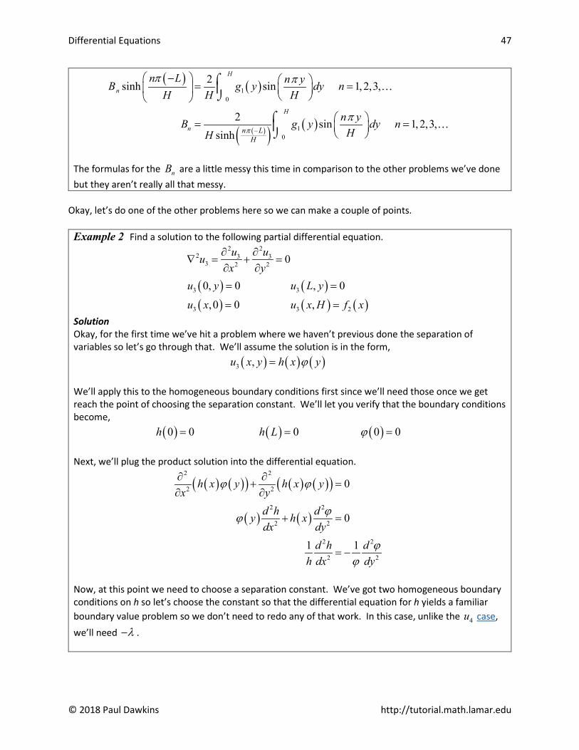
Differential Equations 47
© 2018 Paul Dawkins http://tutorial.math.lamar.edu
( ) ( )
( )( ) ( )
10
10
2sinh sin 1,2,3,
2 sin 1,2,3,sinh
H
n
H
n n LH
n L n yB g y dy nH H H
n yB g y dy nHH π
π π
π−
− = =
= =
⌠⌡
⌠⌡
The formulas for the nB are a little messy this time in comparison to the other problems we’ve done but they aren’t really all that messy.
Okay, let’s do one of the other problems here so we can make a couple of points. Example 2 Find a solution to the following partial differential equation.
( ) ( )( ) ( ) ( )
2 22 3 3
3 2 2
3 3
3 3 2
0
0, 0 , 0
,0 0 ,
u uux y
u y u L y
u x u x H f x
∂ ∂∇ = + =
∂ ∂
= =
= =
Solution Okay, for the first time we’ve hit a problem where we haven’t previous done the separation of variables so let’s go through that. We’ll assume the solution is in the form, ( ) ( ) ( )3 ,u x y h x yϕ= We’ll apply this to the homogeneous boundary conditions first since we’ll need those once we get reach the point of choosing the separation constant. We’ll let you verify that the boundary conditions become, ( ) ( ) ( )0 0 0 0 0h h L ϕ= = = Next, we’ll plug the product solution into the differential equation.
( ) ( )( ) ( ) ( )( )
( ) ( )
2 2
2 2
2 2
2 2
2 2
2 2
0
0
1 1
h x y h x yx y
d h dy h xdx dy
d h dh dx dy
ϕ ϕ
ϕϕ
ϕϕ
∂ ∂+ =
∂ ∂
+ =
= −
Now, at this point we need to choose a separation constant. We’ve got two homogeneous boundary conditions on h so let’s choose the constant so that the differential equation for h yields a familiar boundary value problem so we don’t need to redo any of that work. In this case, unlike the 4u case, we’ll need λ− .

Differential Equations 48
© 2018 Paul Dawkins http://tutorial.math.lamar.edu
This is a good problem in that is clearly illustrates that sometimes you need λ as a separation constant and at other times you need λ− . Not only that but sometimes all it takes is a small change in the boundary conditions it force the change. So, after adding in the separation constant we get,
2 2
2 2
1 1d h dh dx dy
ϕ λϕ
= − = −
and two ordinary differential equations that we get from this case (along with their boundary conditions) are,
( ) ( ) ( )
2 2
2 20 0
0 0 0 0 0
d h dhdx dyh h L
ϕλ λϕ
ϕ
+ = − =
= = =
Now, as we noted above when we were deciding which separation constant to work with we’ve already solved the first boundary value problem. So, the eigenvalues and eigenfunctions for the first boundary value problem are,
( )2
sin 1,2,3,n nn n xh x nL Lπ πλ = = =
The second differential equation is then,
( )
22
2 0
0 0
d ndx Lϕ π ϕ
ϕ
− = =
Because the coefficient of the ϕ is positive we know that a solution to this is,
( ) 1 2cosh sinhn y n yy c cL Lπ πϕ = +
In this case, unlike the previous example, we won’t need to use a shifted version of the solution because this will work just fine with the boundary condition we’ve got for this. So, applying the boundary condition to this gives, ( ) 10 0 cϕ= = and this solution becomes,
( ) 2 sinh n yy cLπϕ =
The product solution for this case is then,
( ), sinh sin 1,2,3,n nn y n xu x y B n
L Lπ π = =
The solution to this partial differential equation is then,

Differential Equations 49
© 2018 Paul Dawkins http://tutorial.math.lamar.edu
( )31
, sinh sinnn
n y n xu x y BL Lπ π∞
=
=
∑
Finally, let’s apply the nonhomogeneous boundary condition to get the coefficients for this solution.
( ) ( )3 21
, sinh sinnn
n H n xu x H f x BL Lπ π∞
=
= =
∑
As we’ve come to expect this is again a Fourier sine (although it won’t always be a sine) series and so using previously done work instead of using the orthogonality of the sines to we see that,
( )
( ) ( )
20
20
2sinh sin 1,2,3,
2 sin 1,2,3,sinh
L
n
L
n n HL
n H n xB f x dx nL L L
n xB f x dx nLL π
π π
π
= =
= =
⌠⌡
⌠⌡
Okay, we’ve worked two of the four cases that would need to be solved in order to completely solve (1). As we’ve seen each case was very similar and yet also had some differences. We saw the use of both separation constants and that sometimes we need to use a “shifted” solution in order to deal with one of the boundary conditions. Before moving on let’s note that we used prescribed temperature boundary conditions here, but we could just have easily used prescribed flux boundary conditions or a mix of the two. No matter what kind of boundary conditions we have they will work the same. As a final example in this section let’s take a look at solving Laplace’s equation on a disk of radius a and a prescribed temperature on the boundary. Because we are now on a disk it makes sense that we should probably do this problem in polar coordinates and so the first thing we need to so do is write down Laplace’s equation in terms of polar coordinates. Laplace’s equation in terms of polar coordinates is,
2
22 2
1 1u uu rr r r r θ∂ ∂ ∂ ∇ = + ∂ ∂ ∂
Okay, this is a lot more complicated than the Cartesian form of Laplace’s equation and it will add in a few complexities to the solution process, but it isn’t as bad as it looks. The main problem that we’ve got here really is that fact that we’ve got a single boundary condition. Namely, ( ) ( ),u a fθ θ= This specifies the temperature on the boundary of the disk. We are clearly going to need three more conditions however since we’ve got a 2nd derivative in both r and θ . When we solved Laplace’s equation on a rectangle we used conditions at the end points of the range of each variable and so it makes some sense here that we should probably need the same kind of conditions here as well. The range on our variables here are,

Differential Equations 50
© 2018 Paul Dawkins http://tutorial.math.lamar.edu
0 r a π θ π≤ ≤ − ≤ ≤ Note that the limits on θ are somewhat arbitrary here and are chosen for convenience here. Any set of limits that covers the complete disk will work, however as we’ll see with these limits we will get another familiar boundary value problem arising. The best choice here is often not known until the separation of variables is done. At that point you can go back and make your choices. Okay, we now need conditions for 0r = and θ π= ± . First, note that Laplace’s equation in terms of polar coordinates is singular at 0r = (i.e. we get division by zero). However, we know from physical considerations that the temperature must remain finite everywhere in the disk and so let’s impose the condition that, ( )0,u θ < ∞ This may seem like an odd condition and it definitely doesn’t conform to the other boundary conditions that we’ve seen to this point, but it will work out for us as we’ll see. Now, for boundary conditions for θ we’ll do something similar to what we did for the 1-D head equation on a thin ring. The two limits on θ are really just different sides of a line in the disk and so let’s use the periodic conditions there. In other words,
( ) ( ) ( ) ( ), , , ,u uu r u r r rr r
π π π π∂ ∂− = − =
∂ ∂
With all of this out of the way let’s solve Laplace’s equation on a disk of radius a. Example 3 Find a solution to the following partial differential equation.
( ) ( ) ( )
( ) ( ) ( ) ( )
22
2 2
1 1 0
0, ,
, , , ,
u uu rr r r r
u u a f
u uu r u r r r
θθ θ θ
π π π πθ θ
∂ ∂ ∂ ∇ = + = ∂ ∂ ∂ < ∞ =
∂ ∂− = − =
∂ ∂
Solution In this case we’ll assume that the solution will be in the form, ( ) ( ) ( ),u r G rθ ϕ θ= Plugging this into the periodic boundary conditions gives,
( ) ( ) ( ) ( )
( )0
d dd d
G
ϕ ϕϕ π ϕ π π πθ θ
− = − =
< ∞
Now let’s plug the product solution into the partial differential equation.
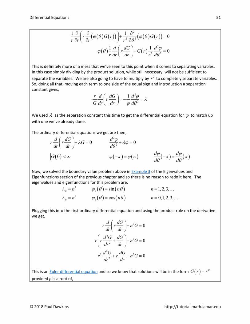
Differential Equations 51
© 2018 Paul Dawkins http://tutorial.math.lamar.edu
( ) ( )( ) ( ) ( )( )
( ) ( )
2
2 2
2
2 2
1 1 0
1 1 0
r G r G rr r r r
d dG dr G rr dr dr r d
ϕ θ ϕ θθ
ϕϕ θθ
∂ ∂ ∂ + = ∂ ∂ ∂
+ =
This is definitely more of a mess that we’ve seen to this point when it comes to separating variables. In this case simply dividing by the product solution, while still necessary, will not be sufficient to separate the variables. We are also going to have to multiply by 2r to completely separate variables. So, doing all that, moving each term to one side of the equal sign and introduction a separation constant gives,
2
2
1r d dG drG dr dr d
ϕ λϕ θ
= − =
We used λ as the separation constant this time to get the differential equation for ϕ to match up with one we’ve already done. The ordinary differential equations we get are then,
( ) ( ) ( ) ( ) ( )
2
20 0
0
d dG dr r Gdr dr d
d dGd d
ϕλ λϕθ
ϕ ϕϕ π ϕ π π πθ θ
− = + =
< ∞ − = − =
Now, we solved the boundary value problem above in Example 3 of the Eigenvalues and Eigenfunctions section of the previous chapter and so there is no reason to redo it here. The eigenvalues and eigenfunctions for this problem are,
( ) ( )( ) ( )
2
2
sin 1, 2,3,
cos 0,1,2,3,n n
n n
n n n
n n n
λ ϕ θ θ
λ ϕ θ θ
= = =
= = =
Plugging this into the first ordinary differential equation and using the product rule on the derivative we get,
2
22
2
22 2
2
0
0
0
d dGr r n Gdr dr
d G dGr r n Gdr dr
d G dGr r n Gdr dr
− =
+ − =
+ − =
This is an Euler differential equation and so we know that solutions will be in the form ( ) pG r r= provided p is a root of,

Differential Equations 52
© 2018 Paul Dawkins http://tutorial.math.lamar.edu
( ) 2
2 2
1 0
0 0,1, 2,3,
p p p n
p n p n n
− + − =
− = ⇒ = ± =
So, because the 0n = case will yield a double root, versus two real distinct roots if 0n ≠ we have two cases here. They are,
( )( )
1 2
1 2
ln 0
1,2,3,n n
G r c c r n
G r c r c r n−
= + =
= + =
Now we need to recall the condition that ( )0G < ∞ . Each of the solutions above will have
( )G r →∞ as 0r → Therefore in order to meet this boundary condition we must have 2 2 0c c= = . Therefore, the solution reduces to, ( ) 1 0,1, 2,3,nG r c r n= = and notice that with the second term gone we can combine the two solutions into a single solution. So, we have two product solutions for this problem. They are,
( ) ( )( ) ( )
, cos 0,1,2,3,
, sin 1,2,3,n n
n n
n
n
u r A r n n
u r B r n n
θ θ
θ θ
= =
= =
Our solution is then the sum of all these solutions or,
( ) ( ) ( )0 1
, cos sinn nn n
n nu r A r n B r nθ θ θ∞ ∞
= =
= +∑ ∑
Applying our final boundary condition to this gives,
( ) ( ) ( ) ( )0 1
, cos sinn nn n
n nu a f A a n B a nθ θ θ θ∞ ∞
= =
= = +∑ ∑
This is a full Fourier series for ( )f θ on the interval π θ π− ≤ ≤ , i.e. L π= . Also note that once again the “coefficients” of the Fourier series are a little messier than normal, but not quite as messy as when we were working on a rectangle above. We could once again use the orthogonality of the sines and cosines to derive formulas for the nA and nB or we could just use the formulas from the Fourier series section with L π= to get,
( )
( ) ( )
( ) ( )
01
21 cos 1,2,3,
1 sin 1,2,3,
nn
nn
A f d
A a f n d n
B a f n d n
π
π
π
π
π
π
θ θπ
θ θ θπ
θ θ θπ
−
−
−
=
= =
= =
∫
∫
∫
Upon solving for the coefficients we get,

Differential Equations 53
© 2018 Paul Dawkins http://tutorial.math.lamar.edu
( )
( ) ( )
( ) ( )
01
21 cos 1,2,3,
1 sin 1,2,3,
n n
n n
A f d
A f n d na
B f n d na
π
π
π
π
π
π
θ θπ
θ θ θπ
θ θ θπ
−
−
−
=
= =
= =
∫
∫
∫
Prior to this example most of the separation of variable problems tended to look very similar and it is easy to fall in to the trap of expecting everything to look like what we’d seen earlier. With this example we can see that the problems can definitely be different on occasion so don’t get too locked into expecting them to always work in exactly the same way. Before we leave this section let’s briefly talk about what you’d need to do on a partial disk. The periodic boundary conditions above were only there because we had a whole disk. What if we only had a disk between say α θ β≤ ≤ . When we’ve got a partial disk we now have two new boundaries that we not present in the whole disk and the periodic boundary conditions will no longer make sense. The periodic boundary conditions are only used when we have the two “boundaries” in contact with each other and that clearly won’t be the case with a partial disk. So, if we stick with prescribed temperature boundary conditions we would then have the following conditions
( )( ) ( )( ) ( )( ) ( )
1
2
0,
,
, 0
, 0
u
u a f
u r g r r a
u r g r r a
θ
θ θ α θ β
α
β
< ∞
= ≤ ≤
= ≤ ≤
= ≤ ≤
Also note that in order to use separation of variables on these conditions we’d need to have
( ) ( )1 2 0g r g r= = to make sure they are homogeneous. As a final note we could just have easily used flux boundary conditions for the last two if we’d wanted to. The boundary value problem would be different, but outside of that the problem would work in the same manner. We could also use a flux condition on the r a= boundary but we haven’t really talked yet about how to apply that kind of condition to our solution. Recall that this is the condition that we apply to our solution to determine the coefficients. It’s not difficult to use we just haven’t talked about this kind of condition yet. We’ll be doing that in the next section.

Differential Equations 54
© 2018 Paul Dawkins http://tutorial.math.lamar.edu
Section 9-8 : Vibrating String This will be the final partial differential equation that we’ll be solving in this chapter. In this section we’ll be solving the 1-D wave equation to determine the displacement of a vibrating string. There really isn’t much in the way of introduction to do here so let’s just jump straight into the example. Example 1 Find a solution to the following partial differential equation.
( ) ( ) ( ) ( )
( ) ( )
2 22
2 2
,0 ,0
0, 0 , 0
u uct x
uu x f x x g xt
u t u L t
∂ ∂=
∂ ∂∂
= =∂
= =
Solution One of the main differences here that we’re going to have to deal with is the fact that we’ve now got two initial conditions. That is not something we’ve seen to this point but will not be all that difficult to deal with when the time rolls around. We’ve already done the separation of variables for this problem, but let’s go ahead and redo it here so we can say we’ve got another problem almost completely worked out. So, let’s start off with the product solution.
( ) ( ) ( ),u x t x h tϕ= Plugging this into the two boundary conditions gives,
( ) ( )0 0 0Lϕ ϕ= = Plugging the product solution into the differential equation, separating and introducing a separation constant gives,
( ) ( )( ) ( ) ( )( )
( ) ( )
2 22
2 2
2 22
2 2
2 2
2 2 2
1 1
x h t c x h tt x
d h dx c h tdt dxd h d
c h dt dx
ϕ ϕ
ϕϕ
ϕ λϕ
∂ ∂=
∂ ∂
=
= = −
We moved the 2c to the left side for convenience and chose λ− for the separation constant so the differential equation for ϕ would match a known (and solved) case. The two ordinary differential equations we get from separation of variables are then,
( ) ( )
2 22
2 20 0
0 0 0
d h dc hdt dx
L
ϕλ λϕ
ϕ ϕ
+ = + =
= =

Differential Equations 55
© 2018 Paul Dawkins http://tutorial.math.lamar.edu
We solved the boundary value problem above in Example 1 of the Solving the Heat Equation section of this chapter and so the eigenvalues and eigenfunctions for this problem are,
( )2
sin 1,2,3,n nn n xx nL Lπ πλ ϕ = = =
The first ordinary differential equation is now,
22
2 0d h n c hdt L
π + =
and because the coefficient of the h is clearly positive the solution to this is,
( ) 1 2cos sinn c t n c th t c cL Lπ π = +
Because there is no reason to think that either of the coefficients above are zero we then get two product solutions,
( )
( )
, cos sin1,2,3,
, sin sin
n n
n n
n c t n xu x t AL L
nn c t n xu x t B
L L
π π
π π
= = =
The solution is then,
( )1
, cos sin sin sinn nn
n c t n x n c t n xu x t A BL L L Lπ π π π∞
=
= + ∑
Now, in order to apply the second initial condition we’ll need to differentiate this with respect to t so,
1
sin sin cos sinn nn
u n c n c t n x n c n c t n xA Bt L L L L L L
π π π π π π∞
=
∂ = − + ∂ ∑
If we now apply the initial conditions we get,
( ) ( ) ( ) ( )
( ) ( )
1 1
1
,0 cos 0 sin sin 0 sin sin
,0 sin
n n nn n
nn
n x n x n xu x f x A B AL L L
u n c n xx g x Bt L L
π π π
π π
∞ ∞
= =
∞
=
= = + = ∂ = = ∂
∑ ∑
∑
Both of these are Fourier sine series. The first is for ( )f x on 0 x L≤ ≤ while the second is for
( )g x on 0 x L≤ ≤ with a slightly messy coefficient. As in the last few sections we’re faced with
the choice of either using the orthogonality of the sines to derive formulas for nA and nB or we could reuse formula from previous work. It’s easier to reuse formulas so using the formulas form the Fourier sine series section we get,

Differential Equations 56
© 2018 Paul Dawkins http://tutorial.math.lamar.edu
( )
( )
0
0
2 sin 1,2,3,
2 sin 1,2,3,
L
n
L
n
n xA f x dx nL L
n c n xB g x dx nL L L
π
π π
= =
= =
⌠⌡
⌠⌡
Upon solving the second one we get,
( )
( )
0
0
2 sin 1,2,3,
2 sin 1,2,3,
L
n
L
n
n xA f x dx nL L
n xB g x dx nn c L
π
ππ
= =
= =
⌠⌡
⌠⌡
So, there is the solution to the 1-D wave equation and with that we’ve solved the final partial differential equation in this chapter.

Differential Equations 57
© 2018 Paul Dawkins http://tutorial.math.lamar.edu
Section 9-9 : Summary of Separation of Variables Throughout this chapter we’ve been talking about and solving partial differential equations using the method of separation of variables. However, the one thing that we’ve not really done is completely work an example from start to finish showing each and every step. Each partial differential equation that we solved made use somewhere of the fact that we’d done at least part of the problem in another section and so it makes some sense to have a quick summary of the method here. Also note that each of the partial differential equations only involved two variables. The method can often be extended out to more than two variables, but the work in those problems can be quite involved and so we didn’t cover any of that here. So with all of that out of the way here is a quick summary of the method of separation of variables for partial differential equations in two variables.
1. Verify that the partial differential equation is linear and homogeneous.
2. Verify that the boundary conditions are in proper form. Note that this will often depend on what is in the problem. So,
a. If you have initial conditions verify that all the boundary conditions are linear and homogeneous.
b. If there are no initial conditions (such as Laplace’s equation) the verify that all but one of the boundary conditions are linear and homogeneous.
c. In some cases (such as we saw with Laplace’s equation on a disk) a boundary condition will take the form of requiring that the solution stay finite and in these cases we just need to make sure the boundary condition is met.
3. Assume that solutions will be a product of two functions each a function in only one of the variables in the problem. This is called a product solution.
4. Plug the product solution into the partial differential equation, separate variables and introduce a separation constant. This will produce two ordinary differential equations.
5. Plug the product solution into the homogeneous boundary conditions. Note that often it will be better to do this prior to doing the differential equation so we can use these to help us chose the separation constant.
6. One of the ordinary differential equations will be a boundary value problem. Solve this to determine the eigenvalues and eigenfunctions for the problem. Note that this is often very difficult to do and in some cases it will be impossible to completely find all eigenvalues and eigenfunctions for the problem. These cases can be dealt with to get at least an approximation of the solution, but that is beyond the scope of this quick introduction.

Differential Equations 58
© 2018 Paul Dawkins http://tutorial.math.lamar.edu
7. Solve the second ordinary differential equation using any remaining homogeneous boundary conditions to simplify the solution if possible.
8. Use the Principle of Superposition and the product solutions to write down a solution to the partial differential equation that will satisfy the partial differential equation and homogeneous boundary conditions.
9. Apply the remaining conditions (these may be initial condition(s) or a single nonhomogeneous boundary condition) and use the orthogonality of the eigenfunctions to find the coefficients. Note that in all of our examples the eigenfunctions were sines and/or cosines however they won’t always be sines and cosines. If the boundary value problem is sufficiently nice (and that’s beyond the scope of this quick introduction to the method) we can always guarantee that the eigenfunctions will be orthogonal regardless of what they are.


