Page 1
Performance of Biogas-Fed Solid Oxide Fuel Cells
A Major Qualifying Project Report submitted to the Faculty of
WORCESTER POLYTECHNIC INSTITUTE
Chemical Engineering Department
in partial fulfillment of the requirements for the Degree of Bachelor of Science
Submitted by:
________________________________
Courtney Jones
April 28, 2016
Advisor: Ravindra Datta
Co-Advisor: Joshua Persky (Protonex)
This report represents the work of WPI undergraduate students submitted to the faculty as evidence
of completion of a degree requirement. WPI routinely publishes these reports on its website without
editorial or peer review. For more information about the projects program at WPI, please see
http://www.wpi.edu/academics/ugradstudies/project-learning.html
Page 2
2
Abstract
Biogas, a renewable fuel produced from organic waste, is commonly used for cooking and
heating in rural or developing communities. The focus of this study was to investigate the use of
this biogas (50-70% CH4 and 20-50% CO2) in a solid oxide fuel cell (SOFC) to produce
electricity. Research in literature has been done on biogas use with button (differential) cells, but
no research has been performed with larger-scale tubular cells, a geometry more indicative of
performance of a larger practical unit. Both humidified and dry biogas compositions were tested
and the cell’s outlet gas composition was analyzed with a mass spectrometer. Stable single-cell
operation was achieved for 250 hours at 12 watts under humidified biogas at 900°C with
minimal degradation. Single cell polarization and durability results were obtained for different
feed gas compositions. Finally, a 5-cell SOFC assembly was tested to simulate a larger practical
unit. A small school in Chhattisgarh, India uses about 465 kWh of electricity per year. One 25-
cell biogas-SOFC stack has the ability to be a primary power source for the school (~2,000
kWh), or be integrated into a solar-SOFC-battery hybrid system.
Page 3
3
Acknowledgements
I would like to first thank my advisors, Ravindra Datta and Joshua Persky, for their guidance and
support with this project. In addition, thank you to Protonex for providing me with endless
resources, from employees’ insights and skills to advanced equipment, that made this project
successful. Thank you to WPI’s chemical engineering department for managing the important
administrative work involved in MQP projects and presentations. Lastly, thank you to WPI for
the opportunity to take part in exciting and meaningful research. The knowledge and skills that I
have gained will be carried with me in all of my future endeavors.
Page 4
4
Table of Contents
Abstract ....................................................................................................................................... 2
Acknowledgements ..................................................................................................................... 3
Table of Contents ........................................................................................................................ 4
Table of Figures .......................................................................................................................... 5
1. Introduction ............................................................................................................................. 6
2. Literature Review.................................................................................................................. 11
2.1 Fuel Cells as an Energy-Producing Technology ............................................................. 11
2.2 Harnessing Biogas .......................................................................................................... 26
2.3 Pairing Biogas with SOFCs ............................................................................................ 30
3. Methodology ......................................................................................................................... 39
3.1 Effect of Biogas Composition on SOFC Performance ................................................... 41
3.2 Effect of Fuel Utilization on SOFC Lifetime ................................................................. 43
3.3 Effect of Moisture in Feed on Cell Lifetime ................................................................... 50
3.4 Mass Spectrometry Analysis on the Outlet Gas of the Single-Cell SOFC ..................... 50
3.4 Effects of 45:55 CH4:CO2 Fuel Through a 5-Cell SOFC Assembly .............................. 53
4. Results and Discussion ......................................................................................................... 55
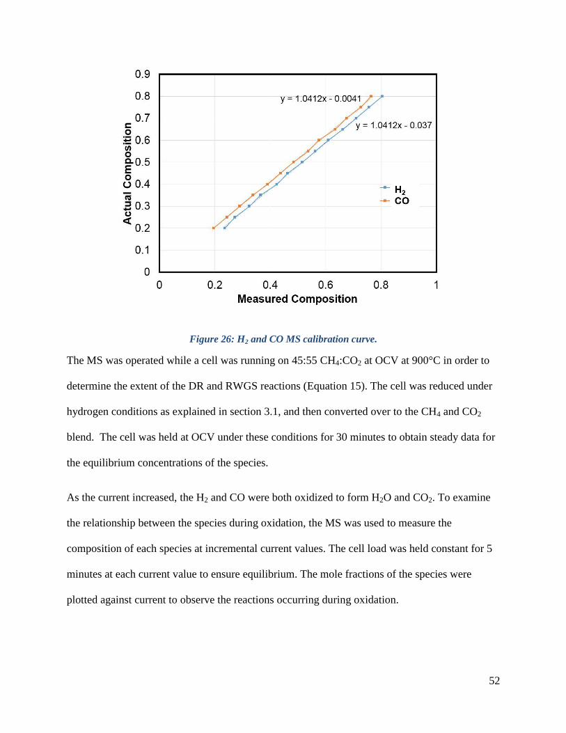
4.1 Effect of Biogas Composition on SOFC Performance ................................................... 55
4.2 Effect of Fuel Utilization on SOFC Lifetime ................................................................. 61
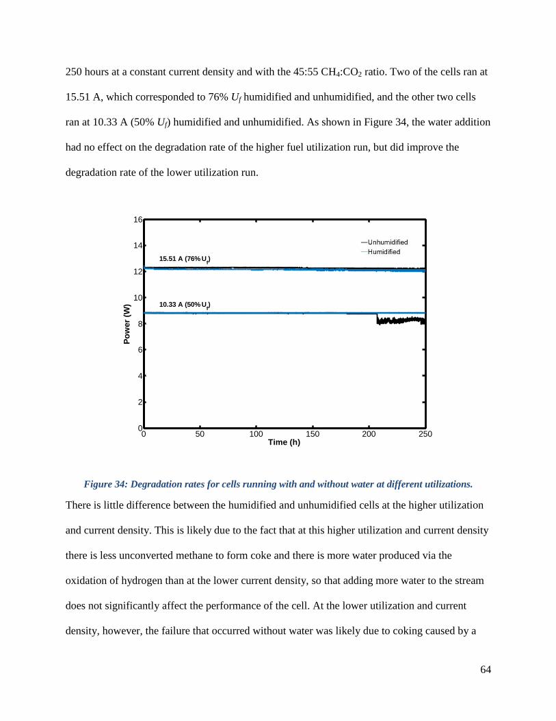
4.3 Effect of Moisture in Feed on Cell Lifetime ................................................................... 63
4.4 Mass Spectrometry Analysis on the Outlet Gas of the Single-Cell SOFC ..................... 65
4.5 Effects of 45:55 CH4:CO2 Fuel Through a 5-Cell SOFC Assembly .............................. 68
5. Conclusions and Commercialization Potential ..................................................................... 70
5.1 Conclusions ..................................................................................................................... 70
5.2 Commercialization Potential ........................................................................................... 70
5.3 Recommendations for Future Work................................................................................ 72
References ................................................................................................................................. 74
Appendices ................................................................................................................................ 78
Appendix A ........................................................................................................................... 78
Appendix B ........................................................................................................................... 79
Appendix C ........................................................................................................................... 84
Page 5
5
Table of Figures
Figure 1: a) Biodigester diagram (Services, 2012), b) Constructed biodigester (The Biodigester,
2014). .............................................................................................................................................. 6 Figure 2: Biodigester-SOFC system flow chart. ............................................................................. 7 Figure 3: Typical tubular solid oxide fuel cells (Tubular, n.d.). ..................................................... 8
Figure 4: Fuel cell market size projection (Fuel Cell Technology, 2014). ................................... 12 Figure 5: Operation of PEMFC or PAFC (Technologies, 2016). ................................................. 14 Figure 6: Operation of AFC (Technologies, 2016). ...................................................................... 16 Figure 7: Operation of MCFC (Technologies, 2016). .................................................................. 17 Figure 8: Operation of SOFC (Technologies, 2016). ................................................................... 18
Figure 9: Plot of low temperature polarization curve with overpotentials (Introduction, 2012). . 20
Figure 10: Polarization plot for pure hydrogen and CO with power density (Homel et al., 2010).
....................................................................................................................................................... 26
Figure 11: Biodigester to cooking stove process (Taherzadeh, 2012). ......................................... 27
Figure 12: Biochemical process of anaerobic digestion (Anaerobic, n.d.). .................................. 28 Figure 13: Effect of temperature on methane production (Vindis and Mursec, 2009). ................ 29 Figure 14: Temperature effect on biogas conversion (Lanzini et al., 2013). ................................ 31
Figure 15: Temperature effect on carbon deposition (Lanzini et al., 2013). ................................ 32 Figure 16: Current required to suppress various amounts of carbon formation (Mermelstein et al.,
2011). ............................................................................................................................................ 35 Figure 17: 800 hour button cell test (Shiratori et al., 2010). ......................................................... 36 Figure 18: a) 500 hour test for 60 mm
3 button cell, b) 500 hour test for 80 mm
3 button cell
(Papadam et al., 2012). ................................................................................................................. 37 Figure 19: Bloom Energy Server
® at Apple's data center (Fehrenbacher, 2013). ........................ 38
Figure 20: PFD for the biogas-SOFC system. .............................................................................. 39 Figure 21: T-SOFC Test Stand Set-Up. ........................................................................................ 40
Figure 22: mks Spectra Products Mass Spectrometer................................................................... 41 Figure 23: Universal Data Acquisition (UDA) Software Interface. ............................................. 43
Figure 24: Gibbs free energy for the DR and RWGS reactions. .................................................. 45 Figure 25: MS capillary in the outlet end of the fuel cell. ............................................................ 51 Figure 26: H2 and CO MS calibration curve. ................................................................................ 52
Figure 27: 5-Cell T-SOFC Assembly. .......................................................................................... 53 Figure 28: Polarization curves for 5 CH4:CO2 ratios and pure H2 and CO. ................................. 56 Figure 29: OCV Values for various CH4:CO2 ratios. ................................................................... 57
Figure 30: Lifetime plot for 60:40 CH4:CO2 at 700°C and 0.7 V. ............................................... 58 Figure 31: Lifetime plots for 4 CH4:CO2 ratios. ........................................................................... 59
Figure 32: Lifetime plots for five different fuel utilizations. ........................................................ 62 Figure 33: Polarization curve for before and after 250 hours of operation at 76% fuel utilization.
....................................................................................................................................................... 63 Figure 34: Degradation rates for cells running with and without water at different utilizations. . 64 Figure 35: Change in composition of species for incremental current values. ............................. 66
Figure 36: H2 and CO composition and respective and total power generation for incremental
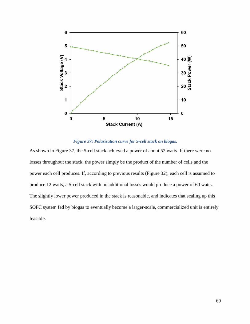
current values. ............................................................................................................................... 68 Figure 37: Polarization curve for 5-cell stack on biogas. ............................................................. 69
Page 6
6
1. Introduction
Methane (CH4) and carbon dioxide (CO2) are two greenhouse gases that are emitted through
anaerobic fermentation of organic waste. This gas mixture is commonly called biogas and
consists of 50-75% CH4, 25-50% CO2, and trace amounts of water (H2O), nitrogen (N2),
hydrogen (H2), and hydrogen sulfide (H2S) (Biogas, n.d.). About 30% of the U.S.’s CH4
emissions in 2013 originated from the biogas produced at landfills and livestock sites (EPA,
n.d.). To prevent these emissions, a common method of harnessing the biogas is with a
biodigester. Biodigesters can be found in rural communities and developing areas of countries
where centralized electricity is impractical or unavailable. Figure 1a shows a diagram of a typical
biodigester, and Figure 1b shows a biodigester that has been implemented in Cambodia.
Figure 1: a) Biodigester diagram (Services, 2012), b) Constructed biodigester (The Biodigester, 2014).
In the 1970s the Chinese government “promoted biogas use in every rural family” and facilitated
the installation of over 7 million biodigesters. These areas, however, primarily use the biogas for
cooking stoves. When biogas is combusted, it produces CO and CO2, leading to high levels of air
Page 7
7
pollution (Bond and Templeton, 2011). These areas could greatly benefit from access to
affordable and reliable technology that allows biogas to directly produce electricity. This study
investigates the use of biogas in a solid-oxide fuel cell (SOFC) to produce electricity.
Fuel cell technology converts chemical energy stored in a fuel to electrical energy to produce
electricity. Most types of fuel cells operate on either H2 or externally reformed fuels to obtain
good performance and to prevent damaging the cell (Fuel Cell Energy, n.d.). However, pure
hydrogen is impractical due to its high cost and difficulty with storage and transportation, and
externally reforming fuels is costly, complex, bulky, and inefficient. Solid oxide fuel cells
(SOFC) relieve these difficulties with their high operating temperature (700 – 1,000 ºC) and thus,
ability to internally reform hydrocarbons and to simultaneously produce utilizable heat
(Protonex, n.d.). Figure 2 shows a flow diagram of a biodigester-SOFC system.
Figure 2: Biodigester-SOFC system flow chart.
The high operating temperature of SOFC provides both advantages and challenges. The former
include high efficiency and direct electro-oxidation of C1 (CO, CH4) molecules at the anode
(McIntosh and Gorte, 2004). The latter include sealing, thermal mismatch, interconnect, and
other material and hardware issues. In fact, the chemistry at the anode is far from certain. Thus,
Page 8
8
depending upon the anode thickness and the amount of Ni present in the anode cermet layer, in
situ reforming of simple C1 fuels such as CH4 occurs, along with water-gas shift reaction,
because of internal recirculation of the water produced via H2 electro-oxidation (Hecht et al.,
2005).
The two most common SOFC structures are tubular and planar. The tubular SOFC (T-SOFC) is
typically stronger than the planar cell in terms of ability to handle both thermal and mechanical
stress. T-SOFC are also advantageous over planar SOFC due to their sealing capabilities. The
ratio of active area to sealing area for a T-SOFC is much greater than that of a planar SOFC,
decreasing the risk of leaks at the site of sealing (Waldemar et al., 2007). Figure 3 shows typical
tubular solid oxide fuel cells.
Figure 3: Typical tubular solid oxide fuel cells (Tubular, n.d.).
Despite the apparent feasibility of a direct biogas-fed SOFC, there is often concern over carbon
deposition at the anode. Carbon deposition is detrimental to SOFC because the solid carbon
deactivates the Ni catalyst by inhibiting the transport of reactants and of electrons at the Ni
surface and can also destroy the anode structure. Thermodynamic analyses have been performed
to determine the possibility of carbon deposition based on fuel composition and operating
temperature. According to Shiratori et al.’s (2010) work on internal dry reforming of biogas
Page 9
9
mixtures, a SOFC fed with a biogas mixture of 50% CH4:50% CO2 should operate around at
least 900˚C to prevent carbon deposition (Shiratori et al., 2010). The high temperature operation
of hydrocarbon-fed SOFCs leads to a high cost of operation. To combat this high cost, research
has been done on external reformation where hydrogen is extracted from the hydrocarbon fuel
before entering the cell. Doing so protects the anode from carbon deposition while allowing
lower operating temperatures. This strategy is effective in decreasing the cost associated with
high-temperature operation, but there are costs associated with external reforming equipment and
operation as well, and the efficiency of the cell is reduced when externally reforming the fuel.
Due to these significant drawbacks with low-temperature operation coupled with external
reforming, the focus of this work is a direct biogas SOFC with a high-temperature operation and
internal reforming.
Previous research has been conducted on the performance of SOFC running on internally
reformed synthetic biogas; however, most of the research is done on small-scale planar button
cells that produce power on the milliwatt scale. For example, a 64 mm2 planar cell operated for
800 hours and produced approximately 100 milliwatts for the duration of the test (Shiratori et al.,
2010). Two cells, 60 mm2 and 80 mm
2 planar cells, were run for about 500 hours each and
produced around 15 and 60 watts for each size cell, respectively (Papadam et al., 2012).
Although both groups obtained results that show the potential of SOFC operating on biogas,
button cell research is limited due to the smaller active area of the cell, as well as the lack of a
concentration gradient over the length of the cell (Standardization, n.d.), causing the results of
the button cell research to be not directly applicable to large-scale SOFC in commercial SOFC
systems. The work performed in this research aims to bridge the gap between the current
Page 10
10
research on small milliwatt-scale fuel cells and larger watt-scale fuel cells that have the potential
to be used in a commercially available SOFC system.
The following chapters include a review of related literature, methodology, results and
discussion, and conclusions. The literature review provides information about both the biogas
and fuel cell industries, and what research has been done thus far to merge the two industries.
The methodology details the methods used to obtain results for the following five objectives:
1. Determine the effects of biogas composition on performance of single SOFC
2. Determine the effects of fuel utilization on lifetime of single SOFC
3. Determine the effects of moisture in feed on SOFC lifetime
4. Analyze the outlet gas composition of single SOFC with mass spectrometer
5. Operate a 5-cell SOFC assembly on synthetic biogas
The results and discussion chapter is broken up based on each of the above objectives. The
conclusions summarize the main findings, and include a discussion of the commercialization
potential of the biogas-fed SOFC studied in this experiment.
Page 11
11
2. Literature Review
To contextualize the issues motivating this project, the literature review here will provide
information about fuel cells and their capabilities, especially in the biofuel industry. The chapter
will begin with an overview of the world’s current energy usage and production, and its effects
on the environment. The chapter then will explain the technical aspects of both solid oxide fuel
cells and biogas. Finally, to provide context for how the work presented in this report fits in to
the current state of the art, the literature review will couple the SOFC and biogas discussion by
summarizing research that has previously been done on feeding biogas through SOFCs.
2.1 Fuel Cells as an Energy-Producing Technology
In a world where the demand for energy is rapidly increasing, discovering clean energy sources
and developing efficient technology to use those resources is critical. Discovered by William
Robert Grove, the “gas battery,” or fuel cell, took off in 1840 when Grove found that he could
generate an electric current by reversing the hydrolysis of water (SAE, 2015). Since then, fuel
cells have been used and tested by NASA on spacecraft, leading car manufacturers, the US
military, and many other industries in an attempt to efficiently produce clean energy. The fuel
cell industry is projected to continue to grow with an industry value of $5.20 billion by 2019.
Further, the number of stationary, portable, and transportation fuel cell shipments is expected to
exceed 200,000 by 2019 (Figure 4)(Fuel Cell Technology, 2014).
2.1.1 Global Energy Status
Energy serves as the foundation for a healthy global economy, providing essential services for
humans around the world. Many countries desire access to energy resources and the technology
that enables them to utilize those resources efficiently in order to improve their economy and
Page 12
12
residents’ quality of lives. Currently, coal, oil, and natural gas (fossil fuels) are the world’s
primary sources of energy accounting for about 75% of the world’s total energy supply. When
burned, however, these fossil energy sources produces the greenhouse gas carbon dioxide (CO2),
along with pollutants such as carbon monoxide (CO) and nitrogen oxides (NOx), leading to high
levels of air pollution (Bond and Templeton, 2011).
Figure 4: Fuel cell market size projection (Fuel Cell Technology, 2014).
The planet’s population is continually increasing and expected to reach nine billion people by
2050 (Population, n.d.), as is their standard of living. These two factors together naturally give
rise to an increasing energy demand for the foreseeable future. The fossil fuel supply is limited,
so continued use without greatly increasing the renewable fuel options could lead to a depletion
of the world’s energy supply while adding to greenhouse gas emissions, a worrisome scenario
for the global economy and climate change. If renewable resources and technologies are not
increasingly utilized, the increasing energy demand has the potential to outweigh the finite fossil
fuel supply, creating a global energy crisis (FAO, n.d.).
Page 13
13
2.1.2 Fuel Cell Operation
Fuel cell technology mitigates the harmful emissions of current energy-producing methods by
producing energy more efficiently and therefore with smaller net quantities of CO2 and CO
emissions. This technology converts the chemical energy present in hydrogen-rich fuels directly
into electrical energy and utilizable heat, unlike conventional methods, where the energy of a
fuel is first converted to thermal energy via combustion, and then into mechanical energy of a
turbine, and finally into electrical energy via an alternator. Fuel cells generally consist of anode
where the fuel reacts electrocatalytically producing electrons that are directed to the external
circuit, and cathode electrodes where the oxidant, usually oxygen from air, gets reduced using
the electrons arriving from the external circuit after performing useful work, and an electrolyte
separating the two electrodes which allows ions produced at the anode or cathode to complete
the circuit.
Other fuels aside from hydrogen may still be used in fuels cells, but some types of fuel cells
require external reforming to convert the non-hydrogen fuel to pure hydrogen or a hydrogen rich
mixture before entering the cell. In all cases, as long as there is fuel and oxygen supply, fuel cells
produce electricity, and thus, unlike batteries, they do not require recharging(Fuel Cell Energy,
n.d.).
2.1.3 Types of Fuel Cells
There are many different types of fuel cells being researched today. Most of the cells are named
by their electrolyte characteristics. Examples include polymer electrolyte fuel cells (PEMFC),
alkaline fuel cells (AFC), phosphoric acid fuel cells (PAFC), molten carbonate fuel cells
(MCFC), and solid oxide fuel cells (SOFC). This section will discuss the basic characteristics of
these 5 types of fuel cells and their advantages and disadvantages (U.S.D.O.E, 2004).
Page 14
14
The first type of fuel cell that will be discussed is the polymer electrolyte fuel cell (PEMFC). The
electrolyte for this type of fuel cell is the ion exchange membrane, which is a solid electrolyte
that conducts protons. This electrolyte requires constant hydration, so the water in the cell must
not evaporate faster than it is produced. This restriction imposes a strict operating temperature
range of 60°C-100°C, with most cells operating between 60°C and 80°C. This also means that
pure H2 is required as a fuel with very low tolerance for CO, which poisons the catalyst. The
anode and cathode catalyst for the PEMFC is generally a platinum-based catalyst. The general
operation of the PEMFC/PAFC is shown in Figure 5 (U.S. D.O.E., 2004). The PAFC instead
utilizes supported phosphoric acid as the electrolyte and operates at higher temperatures (150 –
220 ºC) and so can utilize reformed hydrogen with up to 1% CO directly.
Figure 5: Operation of PEMFC or PAFC (Technologies, 2016).
The most common application for PEMFC is in the fuel cell vehicle (FCV) industry. There is
also PEMFC presence in portable power and small stationary power (U.S. D.O.E., 2004) The
most prominent limiter to additional commercialization of PEMFC is the cost and durability. The
components of a PEMFC are inherently expensive and undergo significant degradation after
about 5,000 hours for lightweight vehicles, and 40,000 hours for small stationary power systems.
Page 15
15
The Department of Energy (DOE) consistently establishes goals to decrease the loading of the
platinum catalyst in the PEMFC, as well as the overall cost to increase its commercialization
potential (Wang et al., 2011).
Overall, there are many advantages to PEMFC. One of these includes fast start-up due to the low
operating temperature. Also, the performance in terms of current and power density is very high.
On the other hand, there are a few disadvantages to PAFC as well. The low operating
temperature only allows the use of hydrogen rather commercially available fuels. Any
contaminants including CO, sulfur, and ammonia are detrimental to the performance of the cell.
In addition, there is currently a lack of hydrogen infrastructure available (U.S. D.O.E., 2004),
and hydrogen, being the lightest element is difficult to efficiently transport and store.
The phosphoric acid fuel cell (PAFC) uses a liquid phosphoric acid as its electrolyte. The acid is
generally concentrated at 100 percent and operates around 150°C-220°. The anode and cathode
are made of a porous carbon material with a platinum catalyst. The operation of PAFCs is
identical to that of the PEFC shown in Figure 5 above.
The efficiency of PAFCs are very high at 85 percent when factoring in electricity plus heat, but
for just electricity, the efficiency is about 37-42 percent, which is only slightly more than that of
a combustion-based conventional heat engine generator. PAFCs have many advantages over
other fuel cells. They have a higher tolerance than PEFCs and AFCs for small amounts of
impurities such as CO, but their low operating temperature still allows for the use of common
and commercially available materials. In addition, PAFCs produce a significant amount of usable
waste heat. There are some disadvantages of PAFCs though. One of these includes the fact that
the phosphoric acid electrolyte is very corrosive, so expensive separators are required in the
Page 16
16
stack. Also, efficient PAFCs still require expensive and complex reformer systems including a
water gas shift reactor when methane is used as the fuel.
Another type of fuel cell is the alkaline fuel cell (AFC). The AFC uses a potassium hydroxide
(KOH) electrolyte soaked into a porous separator. If the cell is operated at high temperatures,
above 250°C, the KOH is concentrated at about 85 wt. percent. If the AFC is operated at lower
temperatures, less than 120°C, the KOH is less concentrated at about 35-50 wt. percent. The
AFC can use a variety of catalysts including nickel, silver, metal oxides, spinels, and noble
metals (U.S. D.O.E., 2004), although Pt is still the most common catalyst employed. The
operation of an AFC is depicted in Figure 6.
Figure 6: Operation of AFC (Technologies, 2016).
The AFC was one of the first fuel cells to be developed. They were developed with a goal of
using them on the Apollo space mission to provide electricity as well as potable water on the
space craft. Unfortunately, for terrestrial applications the AFC is very susceptible to CO2
poisoning, even at very small concentrations such as those in the air, and the CO2 can negatively
affect the performance and lifetime of the fuel cell by reacting with the KOH electrolyte. One of
Page 17
17
the advantages of the AFC is the high rate at which the electrochemical reactions, hydrogen
oxidation reaction (HOR) at the anode, as well as oxygen reduction reaction (ORR) at the
cathode, occur due to the variety of suitable catalysts. When pure hydrogen and oxygen are used,
the AFC can achieve up to 60% efficiency. Despite the potential of the AFC, the CO2 intolerance
requires an extremely precise removal system, an aspect that can significantly increase the cost
and size of an AFC system.
The electrolyte in the molten carbonate fuel cell (MCFC) generally consists of an alkali
carbonate and is operated at high temperatures (600°C-700°C). At these high temperatures, there
is no longer a need for expensive precious metal catalysts at the anode and cathode. The typical
catalysts for an MCFC are nickel at the anode and nickel oxide at the cathode. Because of the
high temperature of operation, the MCFC can utilize fuels other than hydrogen, such as
hydrocarbons, natural gas, and biogas. Figure 7 shows the operation of an MCFC.
Figure 7: Operation of MCFC (Technologies, 2016).
Overall, the advantages of MCFCs include the ability to use inexpensive catalysts and readily
available fuels, and being able to recycle the waste heat from the high temperature cell improves
the efficiency of the cell to be over 50 percent. One of the major disadvantages of the MCFC is
Page 18
18
the corrosiveness of the electrolyte. Also, despite the advantages of the high operating
temperature, the high temperatures introduce problems with materials and stability of the system
(U.S. D.O.E., 2004).
Solid oxide fuel cells (SOFCs) are a highly efficient power-producing system (about 60%
efficiency) (Garrison, n.d.) that operate under very high temperatures (600˚C-1000˚C), allowing
for internal reformation of fuels. Internal reformation allows for more practical fuels than
hydrogen to be used directly in the fuel cell because the fuel does not have to go through
advanced and expensive external reforming. In addition to oxidizing hydrogen, SOFC has the
ability to directly oxidize CO as well (Yi et al., 2005). Figure 8 shows the operation of an SOFC.
Figure 8: Operation of SOFC (Technologies, 2016).
The two most common SOFC structures are tubular and planar. The tubular SOFC (T-SOFC) is
typically stronger than the planar cell in terms of ability to handle both thermal and mechanical
stress, making the tubular cell an excellent match for small-scale and portable systems (Protonex,
n.d.), similar to those that would be implemented alongside biodigesters in small rural
communities. A porous Ni-YSZ (nickel-yttria stabilized zirconia) anode is very common in T-
Page 19
19
SOFCs. Ni-YSZ is relatively inexpensive, robust in high-temperature atmospheres, and displays
similar expansion properties to a YSZ electrolyte. The Ni plays an important role in the
functioning of the cell by serving as an electronic conductor and internal reforming catalyst. The
reforming characteristic is especially important when hydrocarbons, like CH4, are fed directly to
the cell, as the Ni acts as a reforming catalyst when H2, CO, CO2 are produced from the CH4 and
H2O (Hecht et al., 2005).
The SOFC electrolyte must conduct oxide ions and be dense to prevent the passage of gas
molecules. The YSZ electrolyte is a common electrolyte material due to its high oxide ion
conductivity and high density, but it is also not highly conductive electronically so that the
electronic current does not leak from the interconnects (Hecht et al., 2005).
There are many advantages to using SOFCs including the ability to oxidize CO in the cell, the
relatively inexpensive cell materials, and high efficiencies. The disadvantages are generally
associated with the high temperature operation of the cell, as the high temperature poses
problems with thermal expansion and corrosion of various parts of the stack. There are also
difficulties with sealing between planar fuel cells (U.S. D.O.E., 2004).
2.1.5 Fuel Cell Performance Modeling
The three main variables for fuel cell characterization include voltage (V), current (I) or current
density (i), and power (P) or power density. Voltage and current can be measured during the
operation of the fuel cell, and power can be calculated as the product of the voltage and current
as shown in equation 1.
𝑃 = 𝑉 × 𝐼 (1)
Page 20
20
One of the most common ways to characterize the performance of a fuel cell is either with
potentiostatic or galvanostatic techniques. Potentiostatic method involves applying a constant
voltage potential to the cell while measuring the responding current. Galvanostatic is the
opposite; applying a constant current to the cell while measuring the resulting voltage potential.
After conducting an experiment using either of these techniques, a power versus time graph can
be constructed based on the product of the current and voltage results. The purpose of this type
of characterization is to observe the behavior of the cell over time (Olivier, 2008). Potentiostatic
and galvanostatic techniques are especially useful when observing the lifetime of a cell,
especially if it there is a risk of degradation.
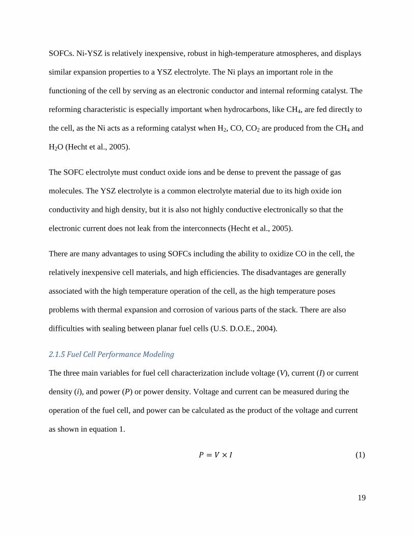
Not only is it beneficial to observe current or voltage over time, but the relationship between
current density and voltage can also present useful information. This relationship is usually
shown in a polarization curve (Figure 9) where the cell voltage is plotted against the current
density, defined as the electric current per cross-sectional area of the cell.
Figure 9: Plot of low temperature polarization curve with overpotentials (Introduction, 2012).
Page 21
21
Polarization curves are helpful when examining the voltage losses associated with the cell.
Figure 9 is an example of a polarization plot for a low temperature fuel cell. The losses
associated with high temperature fuel cells are generally small, and the polarization plot is linear.
On the other hand, in low temperature fuel cells Tafel or logarithmic dependence is observed
between voltage loss and current density for electrode reactions. A fuel cell has an ideal voltage
that is constant with respect to the current density and greater than the actual voltage. Any
deviation from this constant voltage is called over voltage or over potential, and the difference
between the actual voltage and the theoretical voltage is inversely proportional to the cell’s
power output; that is, the smaller the difference between the voltages the greater the cell’s power
output (Rayment, 2003).
The anode, cathode, and overall cell reactions for the case of hydrogen fuel flowing through a
solid oxide fuel cell are as follows:
Electrode Reaction Potential (V) ∆𝐺𝜌𝑜 (kJ/mol) 𝜎𝜌
(2)
Anode: H2 + O2− ⇌ H2O + 2e− 𝛷𝐴,0𝑜 = −0.560 -99.5 +2
Cathode: O2 + 4e− ⇌ 2O2− 𝛷𝐶,0𝑜 = +0.669 -258.2 +1
Overall: 2H2 + O2 ⇌ 2H2O(g) 𝑉0𝑜 = 1.185 -457.4
The thermodynamic data and the corresponding electrode potentials are based on assuming that
the enthalpy of formation of the oxygen anion in YSZ is 𝐻𝑓,O2−(𝑌𝑆𝑍)𝑜 = −85.6 kJ/mol, and
entropy 𝑆𝑓,O2−(𝑌𝑆𝑍)𝑜 = 148.4 J/molK (Goodwin et al., 2009), further assumed to be independent
of temperature, so that 𝐺𝑓,O2−(𝑌𝑆𝑍)𝑜 = −129.1 kJ/mol. It is worth mentioning that these
thermodynamic parameters are not yet known precisely. The water formed is assumed in the
Page 22
22
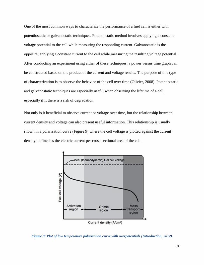
vapor form, i.e., 𝐺𝑓,H2O(𝑔)𝑜 = −228.6 kJ/mol. Further, the Gibbs free energy and hence the cell
thermodynamic potential declines with temperature, i.e.,
𝑉0 = 1.185 − 2.302 × 10⁻⁴(𝑇 − 298) −𝑅𝑇
2𝐹𝑙𝑛
𝑥H22 𝑥O2
𝑥H2O2 (3)
Similarly, for the case of CO fuel, the anode, cathode, and overall cell reactions are
Electrode Reaction Potential (V) ∆𝐺𝜌𝑜 (kJ/mol) 𝜎𝜌
(4)
Anode: CO + O2− ⇌ CO2 + 2e− 𝛷𝐴,0𝑜 = −0.664 -128.1 +2
Cathode: O2 + 4e− ⇌ 2O2− 𝛷𝐶,0𝑜 = +0.669 -258.2 +1
Overall: 2CO + O2 ⇌ 2CO2 𝑉0𝑜 = 1.333 -514.3
And the thermodynamic cell potential in relation to temperature is
𝑉0 = 1.333 − 4.494 × 10⁻⁴(𝑇 − 298) −𝑅𝑇
2𝐹𝑙𝑛
𝑥CO2 𝑥O2
𝑥CO22 (5)
Thus the cell thermodynamic potential declines linearly with temperature for both hydrogen and
carbon monoxide fuel.
At a temperature of 1,000 ºC under hydrogen conditions, thus, this provides, for unit activities or
pure components, a standard thermodynamic potential 𝑉0𝑜 = 0.96 V. The actual thermodynamic
cell voltage is different, as affected by the mole fractions of the species indicated in the
expression above. The OCV is usually lower because of any crossover and internal shorting as
well. The electrolyte in SOFC possesses some electronic conductivity, causing a loss in cell
voltage; however, the electrode kinetics at SOFC temperatures are very rapid, with small
𝑉0𝑜
Page 23
23
overpotentials. The largest potential losses are often due to the electrolyte layer, or due to
diffusion limitations in the electrodes at higher current densities.
The three main types of potential losses that contribute the difference between the actual and
theoretical voltages include activation, Ohmic, and mass transport losses. As shown in Figure 9,
each of these losses occurs at specific current density regions (Rayment, 2003).
The first type of over voltage is called activation losses. These losses occur because the rates of
electrochemical reactions require energy to be enhanced, and at this range of operating
conditions any available energy is used to activate these reactions rather than produce voltage.
High temperatures generally reduce activation losses. Therefore, lower activation losses are
typical for SOFCs due to their high operating temperatures (Rayment, 2003).
Ohmic losses, the second type of over potential, occur due to an Ohmic resistance in the flow of
electrons. Ohmic losses are present in any electrical system and occur in the middle region of
current densities. One way to decrease Ohmic losses is by using electronically-conductive
electrode materials, such as Ni, in the anode, and electrolyte layers with higher ionic
conductivity or smaller thickness. In addition to conductive electrodes, the electrodes should be
short because distance is proportional to resistance, meaning that resistance is increased with
longer electrodes (Rayment, 2003).
The final category of over potential is mass transport loss. This kind of loss occurs due a
decreasing partial pressure or concentration of fuel at either the anode or the cathode. At the
anode, for example, as the cell uses up the available hydrogen, the partial pressure of hydrogen
in the anode decreases, lowering the rate of diffusion and hence the voltage. The same idea is
evident with air pressure at the cathode. In the case of biogas, since CH4 produces double the
Page 24
24
amount of hydrogen than would normally be fed through an SOFC, the mass transfer losses are
expected to be minimal due to an excess amount of hydrogen present at the anode (Rayment,
2003).
As an external current is drawn, as when experimentally producing a polarization curve, the
reduction in potential registered V is equal to V0 minus the sum of the potential drops
overpotentials across all the internal components in series, namely, anode, electrolyte, cathode,
and gas-diffusion layer. Equation 6 shows the relationship between the local current density, the
potential drops, and the resulting overall cell potential (Janardhanan and Deutschmann, 2007)
𝑉 = 𝑉0 − 𝜂𝑎(𝑖) − |𝜂𝑐(𝑖)| − 𝜂𝑜ℎ𝑚(𝑖) − 𝜂𝑐𝑜𝑛𝑐(𝑖) (6)
The anode and cathode (represented respectively by the subscripts a and c) overpotentials are
represented by 𝜂𝑎 and 𝜂𝑐, respectively, and can be calculated via equations 7 and 8.
𝜂𝑎 =2𝑅𝑇
𝑛𝑒𝐹sinh−1 (
𝑖
2𝑖0𝑎) (7)
𝜂𝑐 =2𝑅𝑇
𝑛𝑒𝐹sinh−1 (
𝑖
2𝑖0𝑐) (8)
The local current density is represented by i, and 𝑖0𝑎 and 𝑖0𝑐 are the exchange current densities of
the anode and cathode respectively.
The Ohmic overpotential (𝜂𝑜ℎ𝑚) can be calculated with equation 9,
𝜂𝑜ℎ𝑚 = 𝑖𝑅𝑡𝑜𝑡 (9)
where 𝑅𝑡𝑜𝑡, the total resistance of all of the cell components, can be calculated by equation 10.
𝑅𝑡𝑜𝑡 = 𝜌𝑒𝑙𝑒 + 𝜌𝑎𝑙𝑎 + 𝜌𝑐𝑙𝑐 + 𝑅𝑐𝑜𝑛𝑡𝑎𝑐𝑡 (10)
Page 25
25
In equation 13, the subscript e represents the electrolyte, 𝜌 is the specific electrical resistance of
the cell component (electrolyte, anode, and cathode), l is the component’s thickness, and
𝑅𝑐𝑜𝑛𝑡𝑎𝑐𝑡 is the contact resistance, if any.
The final loss category represented in equation 6 is concentration loss, or 𝜂𝑐𝑜𝑛𝑐. The
concentration loss can be calculated using equation 11,
𝜂𝑐𝑜𝑛𝑐 =𝑅𝑇
𝑛𝑒𝐹𝑙𝑛 (1 −
𝑖
𝑖𝑙) (11)
where 𝑖𝑙 is the limiting current density, when the current is limited completely by diffusional
limitations of the reactant. Figure 10 presents a polarization plot for the case of pure H2 and pure
CO fed to a SOFC.
For the case of pure hydrogen, the standard cell potential, 𝑉0, can be described by equation 6,
and thus, after calculating the losses throughout the cell (equations 7-11), the potential with
respect to any current density can be calculated using equation 9. This calculation would allow
for the creation of a theoretical polarization plot for pure H2. A similar method could be used for
pure CO.
Polarization plots for pure H2 and CO fed SOFC have been provided in the literature, and an
example of one generated at 850 ºC is shown in Figure 10. In addition to the voltage versus
current curve, power versus current density is commonly plotted as well. It is clear from this that
SOFC, owing to its high operating temperatures, is fully capable to electrocatalytically oxidizing
CO directly, while it acts as a poison for the lower temperature fuel cells, which are unable to
electrochemically oxidize CO. Further, the polarization plot for CO is only slightly lower than
that for H2, indicating a key advantage of the high temperature operation of the SOFC. Electrode
kinetics are enhanced by both temperature and by potential as described by the Arrhenius and the
Page 26
26
Butler-Volmer equations, respectively. Therefore, temperature and potential are complementary.
A high operating temperature means lower overpotentials or kinetic potential losses.
Figure 10: Polarization plot for pure hydrogen and CO with power density (Homel et al., 2010).
2.2 Harnessing Biogas
Carbon dioxide (CO2) and methane (CH4) are the two main components of biogas formed from
the anaerobic fermentation of organic waste. As a greenhouse gas, methane is actually 25 times
more damaging to the atmosphere than CO2. In terms of CO2 equivalence over 6,000 million
metric tons of methane were released into the atmosphere in 2013 (EPA, n.d.). However,
methane can be harnessed using effective technology and used as a fuel. Ever since 1970 when
the Chinese government “promoted biogas use in every rural family” and facilitated the
installation of over 7 million biodigesters, about 42 million small-scale household biodigesters
have been built in China and about 4 million in India in an effort to harness biogas. The biogas is
typically used for cooking, lighting, and sometimes with small combustion engines (Bond and
Templeton, 2011). Figure 11 shows this process being utilized in Vietnam.
Page 27
27
Figure 11: Biodigester to cooking stove process (Taherzadeh, 2012).
Organic waste consists of any biodegradable waste from plants, animals, or humans. There are
three possible paths for this waste. One is for the CO2 and CH4 emissions to be released to the
atmosphere and contribute to an increase in greenhouse gas emissions. The second path is for
biogas to be burned and used for heating/cooking, while the third is to be used as a fuel in a fuel
cell to generate power.
A biodigester is the vessel where organic waste undergoes anaerobic digestion to produce biogas.
Biogas consists of mostly CH4 and CO2, and traces of water vapor (H2O), hydrogen sulfide
(H2S), CO, and nitrogen gas (N2). Figure 12 shows the biochemical process of anaerobic
digestion.
Some of the most common feedstocks include agricultural residue, food waste, and animal
byproducts (manure, etc.). In general, the CH4 content in the biogas produced from any kind of
feedstock ranges between 50-80%. This is a large range because there are many factors that
influence the biogas content. One factor is the characteristics of the feedstock. Within the food
waste category, carbohydrates, fats, and proteins produce about 50%, 70%, and 60% CH4,
Page 28
28
respectively (Muzenda, 2014). If a biodigester were to be fed with food waste, the composition
of the biogas would range between 50-70% CH4 depending on the biochemical characteristics of
the waste. In terms of manure, the contents of manure vary depending on the diet of the animal.
Dairy cattle manure, for example, produces biogas with 62% CH4 content, however, beef cattle
produces biogas with 56% CH4 (Cropgen, n.d.). In addition, current research has been focused
on codigestion, where one biodigester operates on different kinds of biowastes (e.g. manure +
food mixtures). El-Mashad et al. (2010) showed that this method increases biogas and CH4
production (Table 1); however, it introduces additional variability in the feedstock, and thus, the
additional variability in the CH4 content of the biogas (El-Mashad and Zhang, 2010).
Figure 12: Biochemical process of anaerobic digestion (Anaerobic, n.d.).
Another cause of inconsistent biogas content is temperature changes. Vindis and Mursec (2009)
performed an experiment on the effect of mesophilic (35-37˚C) versus thermophilic (55-60˚C)
Page 29
29
biodigester temperatures on the CH4 content of the biogas produced from a variety of maize
feedstocks (Figure 13) (Vindis and Mursec, 2009).
Table 1: The effect of co-digestion on methane production in biogas (El-Mashad and Zhang, 2010).
Figure 13: Effect of temperature on methane production (Vindis and Mursec, 2009).
The results of this study showed that the average CH4 content from the mesophilic reactor was
57% and the average CH4 content from the thermophilic reactor was 60.5% (Vindis and Mursec,
2009).
Page 30
30
2.3 Pairing Biogas with SOFCs
Despite the variations that exist in the CH4 content of biogas, the biogas can be fed to an SOFC
to produce power. In order to obtain power from biogas in a SOFC, however, the CH4 needs to
somehow be first converted to H2 and CO. This can be done via either external or internal
reformation. External reformation is a way to convert the CH4 and CO2 to H2/CO before the fuel
enters the cell. This method protects the cell from damage from impurities in the fuel. Despite
this protection, external reformation is a costly procedure and decreases the utilization potential
of the fuel. This limitation leads to the desire for internal reformation, where the fuel is converted
to H2/CO within the cell. In the case of an SOFC, internal reformation can occur readily because
of its high operating temperature and the presence of the Ni catalyst. Thus, CH4 and CO2 in the
biogas reform internally at temperatures above 650˚C to form H2 and CO
CH4 + CO2 → 2CO + 2H2 ∆𝐻 = 247 kJ/mol (12)
In the SOFC, the H2 reacts with the O2-
to form H2O, while the CO reacts with the O2-
to form
CO2 , as described in Chapter 2, and the resulting electrical current produces a useful voltage.
Based on this hypothesis, biogas, in theory, is a suitable feed for an SOFC.
Lanzini et al. (2013) confirmed this theory experimentally by showing that as temperature
increased above about 500°C the conversion of CO2 and CH4 increased due to enhanced kinetics,
producing more CO and H2 (Figure 14) (Lanzini et al., 2013). At around 850°C, however, the
conversion plateaued suggesting that maximum conversion of CH4 and CO2 occurs at
temperatures around 850°C (Lanzini et al., 2013), conceivably because of thermodynamic
limitations. This is discussed in more detail later on in this report.
Page 31
31
Figure 14: Temperature effect on biogas conversion (Lanzini et al., 2013).
2.3.1 Carbon Deposition Damaging the SOFC Anode
Despite the apparent feasibility of a direct biogas-fed SOFC, there is a major concern over
carbon deposition at the anode. The occurrence of one or more of the following three reactions is
possible whenever hydrocarbons or CO are fed through an SOFC:
2CO → C + CO2 (13)
CH4 → C + 2H2 (14)
CO + H2 → C + H2O (15)
Carbon deposition is detrimental to an SOFC because the solid carbon inhibits the transfer of
reactants and electrons across the Ni surface of the anode, and also possibly dislodges the Ni
particles from the anode matrix. Thermodynamic analyses have been performed to determine the
possibility of carbon deposition based on fuel composition and reaction temperature.
Assabumrungrat et al. (2006) showed that as the ratio of CH4:CO2 entering the cell increased, the
Page 32
32
carbon activity also increased. This trend occurred at 900K, 950K, 1000K, 1050K, and 1100K,
but if the carbon activity were to remain constant at 900K and 1100K, there would be a higher
tolerance for a greater CH4:CO2 ratio at 1100K than 900K, suggesting that a higher operating
temperature decreases the amount of carbon deposition (Assabumrungrat et al., 2006).
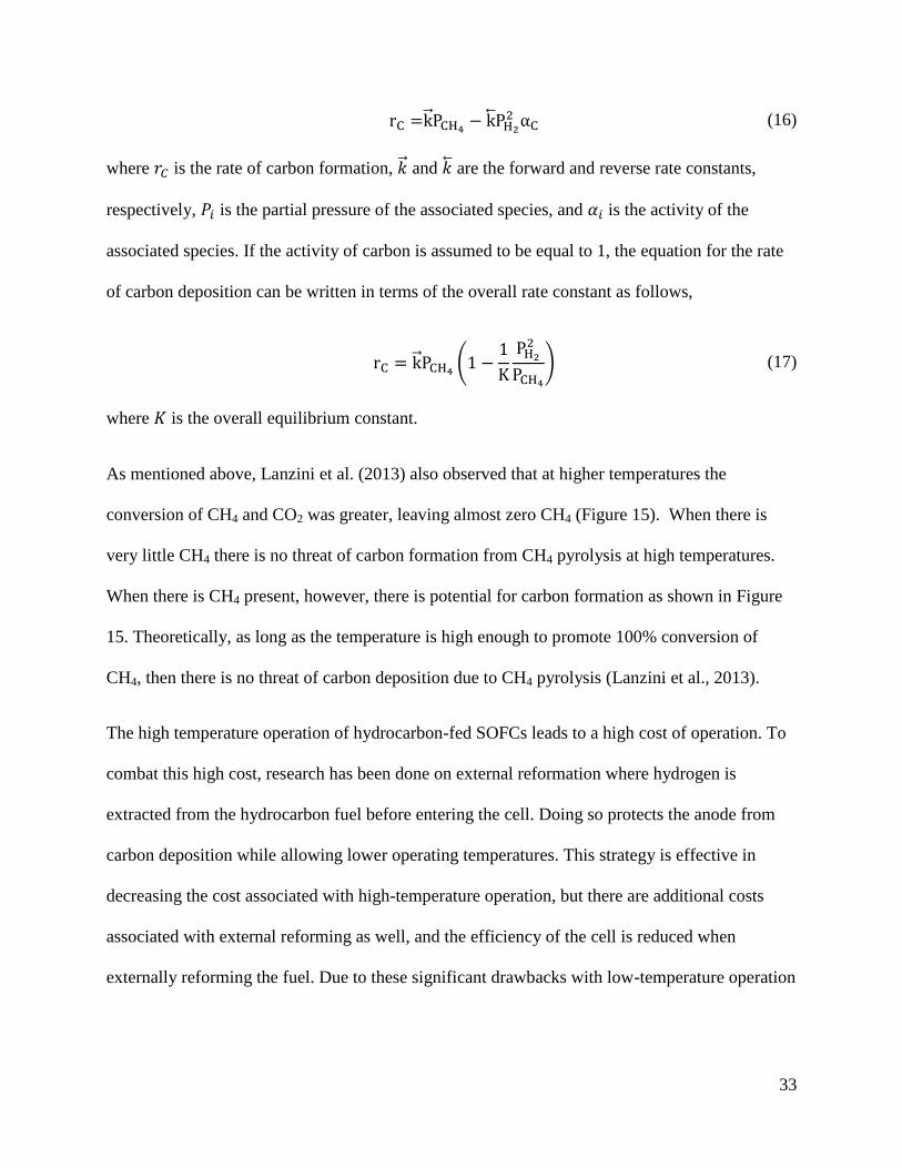
For the case of pure methane, on the other hand, Lanzini et al. (2013) observed how temperature
affected carbon deposition on a Ni-YSZ anode support by flowing pure methane through the
anode, varying the temperature, and measuring the outlet oxygen, CO2, and CO concentrations,
as well as the amount of carbon on the anode. As shown in Figure 15, the results of this study
suggest at higher temperatures (above 500°C), methane was more likely to form carbon deposits
than at the lower temperatures (Lanzini et al., 2013).
Figure 15: Temperature effect on carbon deposition (Lanzini et al., 2013).
Clearly, the presence of CO2 along with methane in biogas affects the formation of coke.
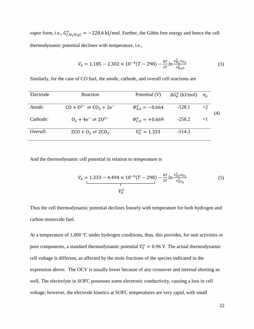
For the case of pure methane feed, the rate of carbon formation by the carbon deposition reaction
(equation 14) can be represented by (Fogler, 2008),
Page 33
33
rC =k PCH4− kPH2
2 αC (16)
where 𝑟𝐶 is the rate of carbon formation, �� and �� are the forward and reverse rate constants,
respectively, 𝑃𝑖 is the partial pressure of the associated species, and 𝛼𝑖 is the activity of the
associated species. If the activity of carbon is assumed to be equal to 1, the equation for the rate
of carbon deposition can be written in terms of the overall rate constant as follows,
rC = k PCH4(1 −
1
K
PH2
2
PCH4
) (17)
where 𝐾 is the overall equilibrium constant.
As mentioned above, Lanzini et al. (2013) also observed that at higher temperatures the
conversion of CH4 and CO2 was greater, leaving almost zero CH4 (Figure 15). When there is
very little CH4 there is no threat of carbon formation from CH4 pyrolysis at high temperatures.
When there is CH4 present, however, there is potential for carbon formation as shown in Figure
15. Theoretically, as long as the temperature is high enough to promote 100% conversion of
CH4, then there is no threat of carbon deposition due to CH4 pyrolysis (Lanzini et al., 2013).
The high temperature operation of hydrocarbon-fed SOFCs leads to a high cost of operation. To
combat this high cost, research has been done on external reformation where hydrogen is
extracted from the hydrocarbon fuel before entering the cell. Doing so protects the anode from
carbon deposition while allowing lower operating temperatures. This strategy is effective in
decreasing the cost associated with high-temperature operation, but there are additional costs
associated with external reforming as well, and the efficiency of the cell is reduced when
externally reforming the fuel. Due to these significant drawbacks with low-temperature operation
Page 34
34
and external reforming, attention will be given to high-temperature operation and internal
reforming in this research.
2.3.2 Higher Current Density Decreases Carbon Deposition
In order to have internal reforming of the biogas, the conditions must be ideal, causing very little
carbon deposition on the anode. Many researchers have claimed anode failure to be due to
carbon deposition, and because of this threat, much research has been done on internal steam
reforming. Internal steam reforming is beneficial to the cell in a couple ways. First, any excess
CH4 entering the cell can react with H2O and form CO and H2, two species that are readily
electrochemically oxidized in a SOFC. This reaction prevents any excess CH4 from breaking
down into C and H2. Secondly, the water present in the cell can also clean out any carbon that
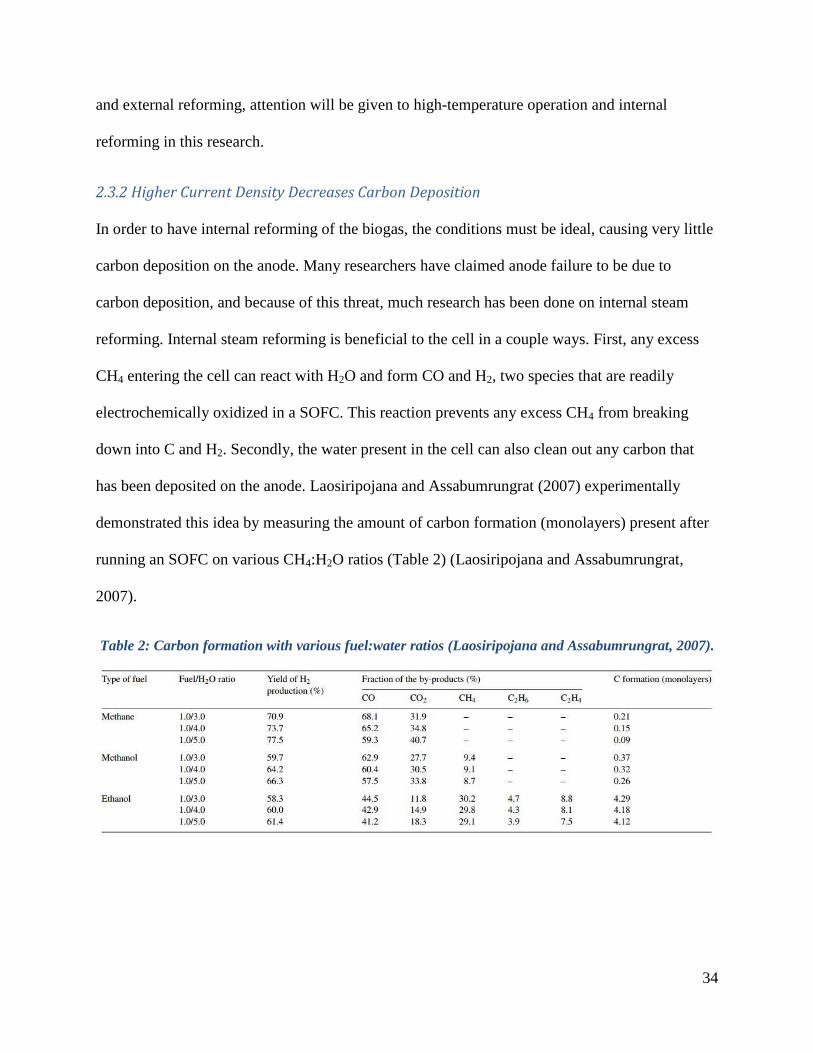
has been deposited on the anode. Laosiripojana and Assabumrungrat (2007) experimentally
demonstrated this idea by measuring the amount of carbon formation (monolayers) present after
running an SOFC on various CH4:H2O ratios (Table 2) (Laosiripojana and Assabumrungrat,
2007).
Table 2: Carbon formation with various fuel:water ratios (Laosiripojana and Assabumrungrat, 2007).
Page 35
35
Their work showed that of the three CH4:H2O ratios (1:3, 1:4, 1:5), the 1:5 ratio produced the
least amount of carbon, suggesting that the increase in steam in the cell decreased the presence of
carbon in the cell (Laosiripojana and Assabumrungrat, 2007).
It is predicted that running the cell at higher current densities will decrease the presence of
carbon in the cell for two reasons. First, by increasing the current density, the partial pressure of
steam in the cell also increases because more hydrogen is being oxidized and generating water
according to equation 2 above. Kinetically, the oxidation of H2 and CO occurs before the
oxidation of carbon, but Mermelstein et al. (2011) experimentally demonstrated that less carbon
deposition was found in the cell when running a cell on higher current density (Figure 16),
suggesting that the carbon can be oxidized as well (Mermelstein et al., 2011).
Figure 16: Current required to suppress various amounts of carbon formation (Mermelstein et al.,
2011).
Page 36
36
Running a cell on high current density or under higher partial pressure of water has the potential
to promote to steam reforming and oxidization of carbon deposits, and thus decrease the amount
of carbon deposition in the cell.
2.3.3 Lack of Larger-Scale, Tubular SOFC Research with Biogas
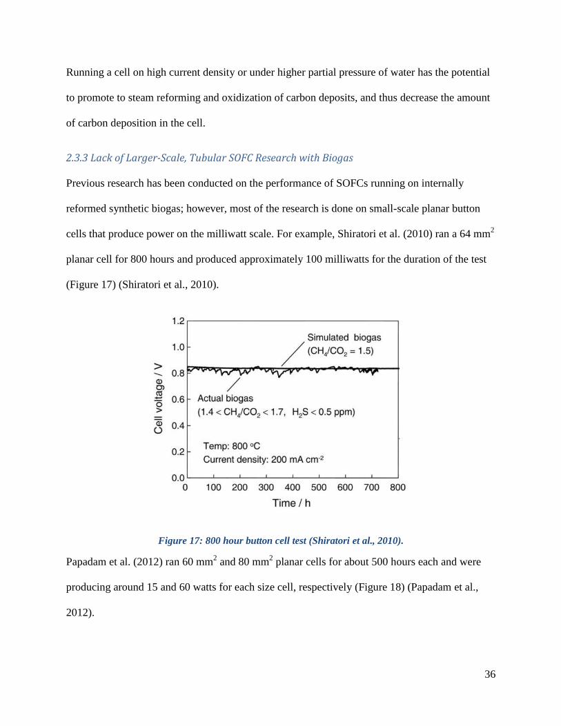
Previous research has been conducted on the performance of SOFCs running on internally
reformed synthetic biogas; however, most of the research is done on small-scale planar button
cells that produce power on the milliwatt scale. For example, Shiratori et al. (2010) ran a 64 mm2
planar cell for 800 hours and produced approximately 100 milliwatts for the duration of the test
(Figure 17) (Shiratori et al., 2010).
Figure 17: 800 hour button cell test (Shiratori et al., 2010).
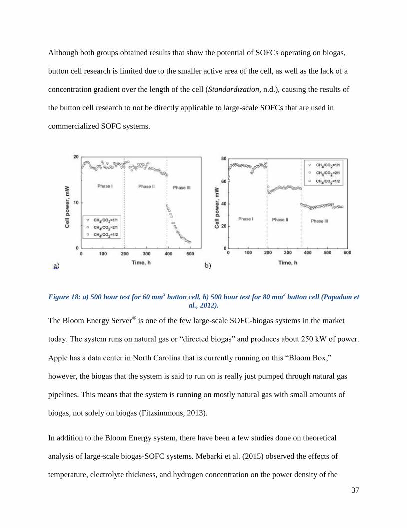
Papadam et al. (2012) ran 60 mm2 and 80 mm
2 planar cells for about 500 hours each and were
producing around 15 and 60 watts for each size cell, respectively (Figure 18) (Papadam et al.,
2012).
Page 37
37
Although both groups obtained results that show the potential of SOFCs operating on biogas,
button cell research is limited due to the smaller active area of the cell, as well as the lack of a
concentration gradient over the length of the cell (Standardization, n.d.), causing the results of
the button cell research to not be directly applicable to large-scale SOFCs that are used in
commercialized SOFC systems.
Figure 18: a) 500 hour test for 60 mm3 button cell, b) 500 hour test for 80 mm
3 button cell (Papadam et
al., 2012).
The Bloom Energy Server® is one of the few large-scale SOFC-biogas systems in the market
today. The system runs on natural gas or “directed biogas” and produces about 250 kW of power.
Apple has a data center in North Carolina that is currently running on this “Bloom Box,”
however, the biogas that the system is said to run on is really just pumped through natural gas
pipelines. This means that the system is running on mostly natural gas with small amounts of
biogas, not solely on biogas (Fitzsimmons, 2013).
In addition to the Bloom Energy system, there have been a few studies done on theoretical
analysis of large-scale biogas-SOFC systems. Mebarki et al. (2015) observed the effects of
temperature, electrolyte thickness, and hydrogen concentration on the power density of the
Page 38
38
SOFC. The biogas characteristics were calculated based on the biogas production at a landfill in
Batna, Algeria. The study assumed an efficiency for the SOFC system of 50%. The optimum
temperature, electrolyte thickness, and hydrogen concentration are 1273 K, 0.1 mm, and >0.5,
respectively. Although this theoretical study does consider large-scale systems, there is still a
lack of experimental data. In contrast to theoretical studies, experimental studies on large-scale
systems allow working through practical problems encountered with the system (Mebarki et al.,
2015).
Figure 19: Bloom Energy Server® at Apple's data center (Fehrenbacher, 2013).
The work performed in this research, therefore, aims to bridge the gap between the reported
experimental research on small milliwatt-scale SOFCs fed with biogas, and larger watt-scale
reactors that have the potential to be used in a commercially available SOFC system.
Page 39
39
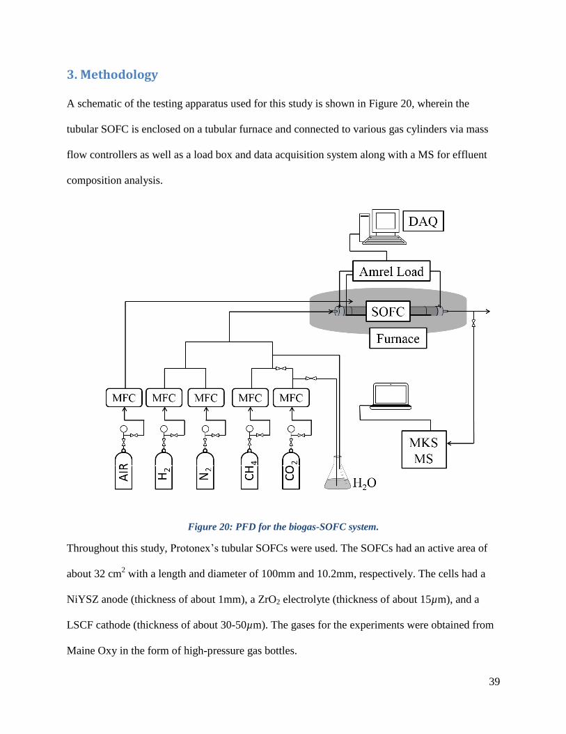
3. Methodology
A schematic of the testing apparatus used for this study is shown in Figure 20, wherein the
tubular SOFC is enclosed on a tubular furnace and connected to various gas cylinders via mass
flow controllers as well as a load box and data acquisition system along with a MS for effluent
composition analysis.
Figure 20: PFD for the biogas-SOFC system.
Throughout this study, Protonex’s tubular SOFCs were used. The SOFCs had an active area of
about 32 cm2 with a length and diameter of 100mm and 10.2mm, respectively. The cells had a
NiYSZ anode (thickness of about 1mm), a ZrO2 electrolyte (thickness of about 15µm), and a
LSCF cathode (thickness of about 30-50µm). The gases for the experiments were obtained from
Maine Oxy in the form of high-pressure gas bottles.
Page 40
40
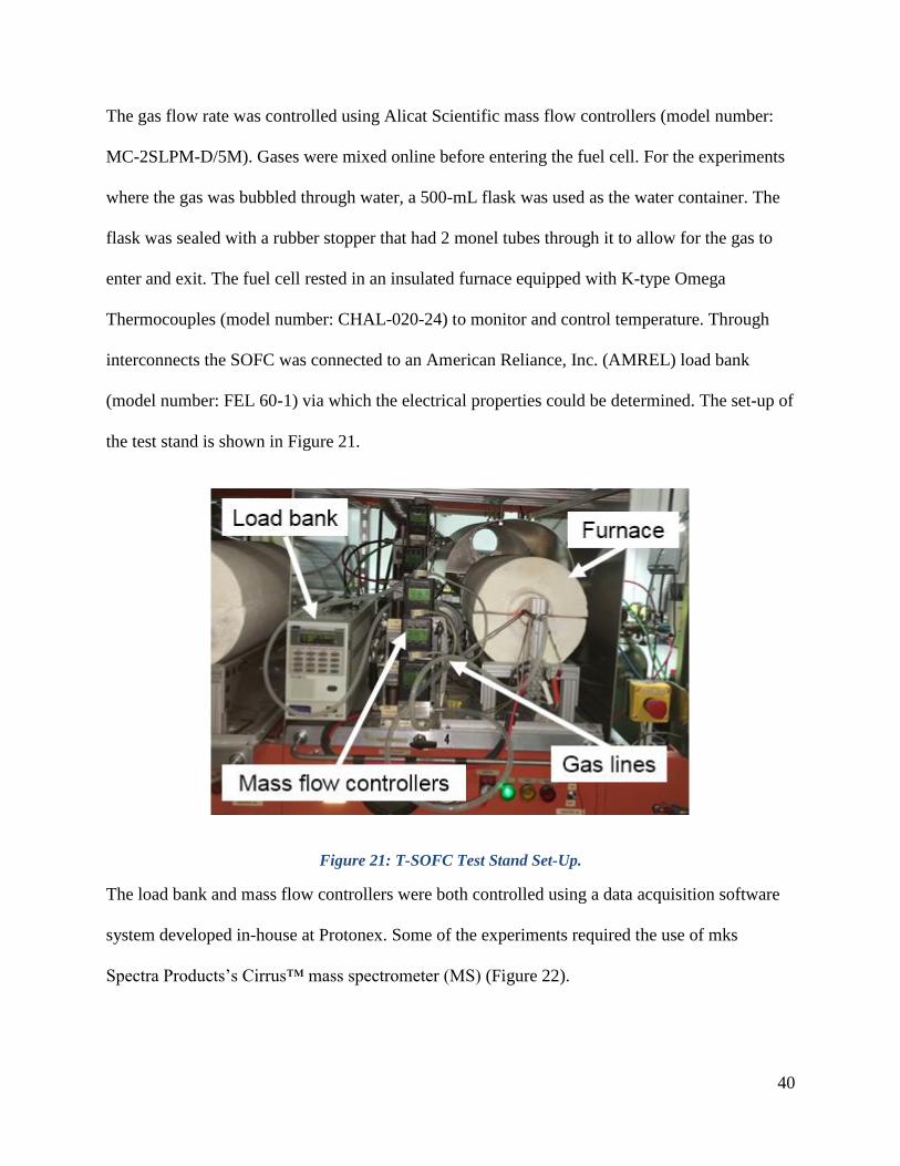
The gas flow rate was controlled using Alicat Scientific mass flow controllers (model number:
MC-2SLPM-D/5M). Gases were mixed online before entering the fuel cell. For the experiments
where the gas was bubbled through water, a 500-mL flask was used as the water container. The
flask was sealed with a rubber stopper that had 2 monel tubes through it to allow for the gas to
enter and exit. The fuel cell rested in an insulated furnace equipped with K-type Omega
Thermocouples (model number: CHAL-020-24) to monitor and control temperature. Through
interconnects the SOFC was connected to an American Reliance, Inc. (AMREL) load bank
(model number: FEL 60-1) via which the electrical properties could be determined. The set-up of
the test stand is shown in Figure 21.
Figure 21: T-SOFC Test Stand Set-Up.
The load bank and mass flow controllers were both controlled using a data acquisition software
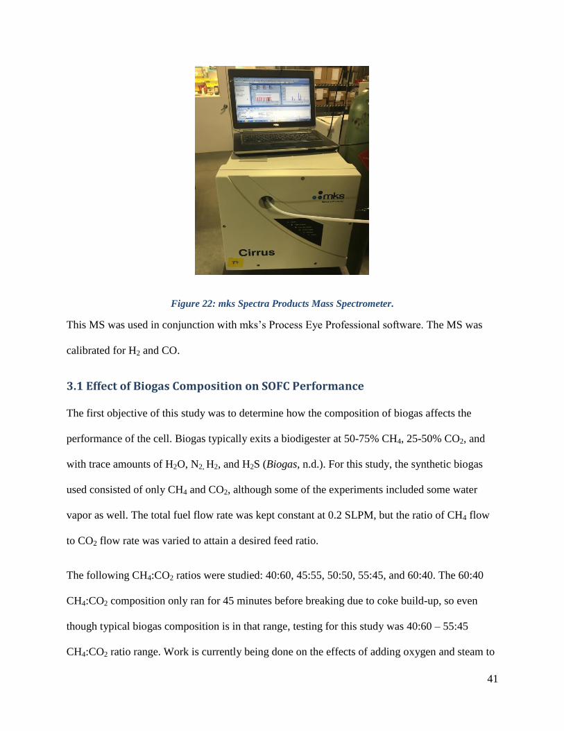
system developed in-house at Protonex. Some of the experiments required the use of mks
Spectra Products’s Cirrus™ mass spectrometer (MS) (Figure 22).
Page 41
41
Figure 22: mks Spectra Products Mass Spectrometer.
This MS was used in conjunction with mks’s Process Eye Professional software. The MS was
calibrated for H2 and CO.
3.1 Effect of Biogas Composition on SOFC Performance
The first objective of this study was to determine how the composition of biogas affects the
performance of the cell. Biogas typically exits a biodigester at 50-75% CH4, 25-50% CO2, and
with trace amounts of H2O, N2, H2, and H2S (Biogas, n.d.). For this study, the synthetic biogas
used consisted of only CH4 and CO2, although some of the experiments included some water
vapor as well. The total fuel flow rate was kept constant at 0.2 SLPM, but the ratio of CH4 flow
to CO2 flow rate was varied to attain a desired feed ratio.
The following CH4:CO2 ratios were studied: 40:60, 45:55, 50:50, 55:45, and 60:40. The 60:40
CH4:CO2 composition only ran for 45 minutes before breaking due to coke build-up, so even
though typical biogas composition is in that range, testing for this study was 40:60 – 55:45
CH4:CO2 ratio range. Work is currently being done on the effects of adding oxygen and steam to
Page 42
42
a more typical simulated biogas composition (60:40 CH4:CO2) to drive down the methane
composition entering the cell, and maintain a high lifetime.
For this objective, the fuel utilization, i.e., the ratio of actual current applied to maximum
possible current density based on the amount of fuel, was maintained at a modest 50% to prevent
any issues due to a fuel utilization that was either too high or too low. For this objective, the fuel
utilization was calculated simply by determining the maximum current that would result if all of
the methane were converted to hydrogen, and taking 50% of that value. This calculation was
suitable for this experiment, but a more accurate calculation based on equilibrium conversion of
the reactants was used and described with Objective 2.
Once the SOFC was placed in the furnace, the cell was heated to 900°C with hydrogen flowing
through the cell. A temperature of 900°C was chosen due to the desire to maximize conversion
of CH4, and thus, minimize coking, as described in section 2.3.1. The temperature of the cell was
maintained at 900°C for 3 hours to reduce the nickel (II) oxide on the anode to nickel under the
hydrogen atmosphere. Once the reducing procedure was complete, the cell ran under constant
current density for 1 hour so that a comparison could be made between the biogas results and the
hydrogen. Following the constant current density, polarization plot data was obtained for the cell
under hydrogen conditions. After the polarization plot, the inlet fuel transitioned from hydrogen
to simulated biogas. To allow for the cell to remain at 900°C, the hydrogen was not shut off until
the methane and carbon dioxide were flowing through the cell. Once the hydrogen was off, a
polarization plot was obtained under biogas conditions, and then the constant current density
conditions were set and the fuel cell run under these conditions for 150 hours to determine
stability and durability. The shut-down procedure involved cooling the cell while hydrogen
flowed through the cell. This procedure was used for each of the 5 CH4:CO2 ratios studied in this
Page 43
43
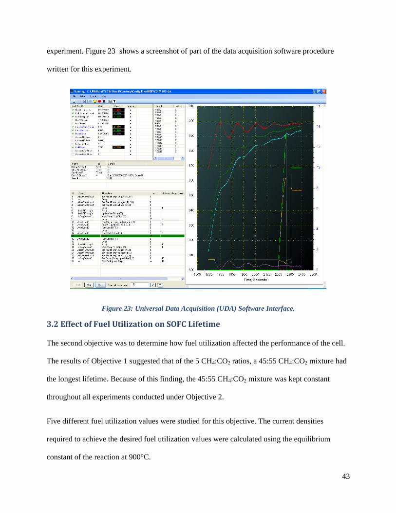
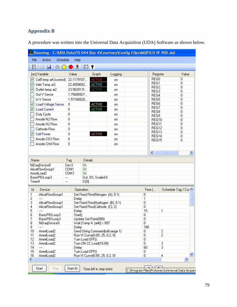
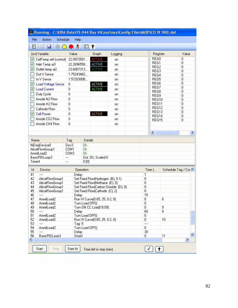
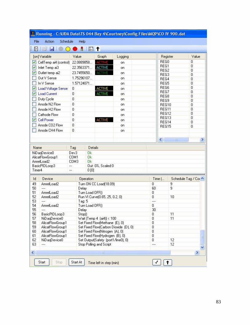
experiment. Figure 23 shows a screenshot of part of the data acquisition software procedure
written for this experiment.
Figure 23: Universal Data Acquisition (UDA) Software Interface.
3.2 Effect of Fuel Utilization on SOFC Lifetime
The second objective was to determine how fuel utilization affected the performance of the cell.
The results of Objective 1 suggested that of the 5 CH4:CO2 ratios, a 45:55 CH4:CO2 mixture had
the longest lifetime. Because of this finding, the 45:55 CH4:CO2 mixture was kept constant
throughout all experiments conducted under Objective 2.
Five different fuel utilization values were studied for this objective. The current densities
required to achieve the desired fuel utilization values were calculated using the equilibrium
constant of the reaction at 900°C.
Page 44
44
Due to the presence of Ni catalyst and the high operating temperature (900 ºC), we can assume
that there is gas-phase reaction equilibrium in effect among the gas-phase species at the tube exit.
There are n = 6 species (CH4, CO2, CO, H2, H2O, and C), and e = 3 elements. Thus, the number
of independent overall reactions (ORs) needed for a thermodynamic or kinetic analysis is μ = n –
e = 3. Any set of 3 independent ORs would suffice for this purpose. Therefore, we may pick the
following set:
OR1: CH4 + CO2 ⇌ 2CO + 2H2 ∆𝐻1𝑜 = +247 (kJ/mol) (DR)
OR2: H2 + CO2 ⇌ CO + H2O ∆𝐻2𝑜 = +41 (kJ/mol) (RWGS) (18)
OR3: 2CO ⇌ CO2 + C ∆𝐻1𝑜 = +75 (kJ/mol) (Coking)
From the standard thermodynamic data for these species at 298 K:
Species 𝐻𝑖,298𝑜 (kJ/mol) 𝑆𝑖,298
𝑜 (J/molK) 𝐺𝑖,298𝑜 (kJ/mol)
CH4 -74.852 186.27 -50.836
H2O -241.818 188.72 -228.589
CO2 -393.505 213.67 -394.384 (19)
CO -110.541 197.90 -137.277
H2 0 130.59 0
C 0 5.694 0
O2 0 205.00 0
Further assuming the species entropy and enthalpy of formation to be constant with temperature
and using ∆𝐺𝑂𝑅𝑜 = ∆𝐻𝑂𝑅
𝑜 − 𝑇∆𝑆𝑂𝑅𝑜 , the standard Gibbs free energy of the above three ORs may
Page 45
45
be plotted as a function of temperature to determine their operating temperatures of feasibility,
i.e., when the ∆𝐺𝑂𝑅𝑜 < 0. An example of such a plot is provided (Figure 24).
Figure 24: Gibbs free energy for the DR and RWGS reactions.
Further, from
𝐾𝑂𝑅 = 𝑒𝑥𝑝 (−∆𝐺𝑂𝑅
𝑜
𝑅𝑇) = 𝑒𝑥𝑝 (−
∆𝑆𝑂𝑅𝑜
𝑅𝑇)𝑒𝑥𝑝 (−
∆𝐻𝑂𝑅𝑜
𝑅𝑇) (20)
we can write
𝐾𝑂𝑅 = 𝐾𝑂𝑅,298𝑒𝑥𝑝 {−∆𝐻𝑂𝑅
𝑜
𝑅𝑇(1
𝑇−
1
298)} (21)
for the above three equations and writing these in terms of 1, 2, and 3, the equilibrium
conversions for the three ORs, the feed gas ratio, and the current drawn, one can solve for these
three independent nonlinear equations via root finding (e.g., Newton’s method, using Maple or
Mathematica, etc.). This would correspond to the exit conditions in the absence of current
Page 46
46
assuming reaction equilibrium is attained inside the SOFC tube, so that the exit gas composition
can be determined.
If C is neglected, only 2 equations are needed. Let us analyze this case first, as at any rate the
amount converted to C is small. Then from the above data for the DRR
∆𝐻𝐴1𝑜 = +247.275 kJ/mol
∆𝑆𝐴1𝑜 = +257.04 J/mol-K (22)
∆𝐺𝐴1𝑜 = +170.669 kJ/mol
where A in the subscript refers to anode, and 1 alludes to OR1. In other words, the reaction is
highly endothermic and endergonic at room temperature, with the reaction equilibrium constant
being virtually zero for the DR reaction. Actually,
𝐾𝐴1,298 = 𝑒𝑥𝑝 (−∆𝐺𝐴1,298
𝑜
𝑅𝑇) = 1.25 × 10⁻³⁰. However, at 900ºC, the reaction becomes quite
exergonic owing to the change in Gibbs free energy with temperature, and 𝐾𝐴1,1173 = 257.75.
Similarly for the RWGSR, the standard Gibbs free energy and enthalpy of the reaction are given
by
∆𝐻𝐴2𝑜 = +41.146 kJ/mol
∆𝑆𝐴2𝑜 = +42.36 J/mol-K (23)
∆𝐺𝐴2𝑜 = +28.518 kJ/mol
In other words, the reaction is endothermic and endergonic at room temperature, with the
reaction equilibrium constant being 𝐾𝐴2,298 = 𝑒𝑥𝑝 (−∆𝐺𝐴2,298
𝑜
𝑅𝑇) = 1.0 × 10⁻⁵. However, at
900ºC, the reaction becomes exergonic, and 𝐾𝐴2,1173 = 2.40.
Page 47
47
With the equilibrium constants being determined at 900ºC, the extents of the two reactions can
next be determined, from which the equilibrium gas composition can be determined as follows.
Recall that the molar flow rate ��𝑖 of a species i in a flow reactor is related to the q independent
reaction extents ��𝜌 ≡ ∫ 𝑟𝜌𝑑𝑉𝑉
as follows (Fogler, 4
th ed.)
��𝑖 = ��𝑖,0 + ∑ 𝜈𝜌𝑖��𝜌
𝑞
𝜌=1
(i = 1, 2, …, n) (24)
Summing these over all species, the total molar flow rate
��𝑇 = ��𝑇,0 (1 + 𝜒𝐴0 ∑ ∆𝜈𝜌𝜒𝜌
𝑞
𝜌=1
) (25)
where 𝜒𝐴0 is the feed mole fraction of the key reactant A (CH4), and the change in the number of
moles in reaction ρ, ∆𝜈𝜌, and the dimensionless reaction extent 𝜒𝜌 are defined by the following
��𝜌 = ∑𝜈𝜌𝑖
𝑛
𝑖=1
𝜒𝜌 ≡��𝜌
��𝐴,0 (ρ = 1, 2, …, n) (26)
where ��𝐴,0 is the feed molar flow rate of the key reactant A (CH4).
Finally, the mole fraction of the species, 𝑥𝑖 =��𝑖
��𝑇
𝑥𝑖 =𝛩𝑖 + ∑ 𝜈𝜌𝑖𝜒𝜌
𝑞𝜌=1
1𝑥A0
+ ∑ ∆𝜈𝜌𝜒𝜌𝑞𝜌=1
(i = 1, 2, …, n) (27)
where the molar feed ratio of species i, 𝛩 ≡��𝑖,0
��𝐴,0.
Page 48
48
This provides the following mole fractions for the five species participating in the two non-
electrocatalytic electrode reactions, namely the DRR and the RWGSR. Here ∆𝜈𝐷𝑅𝑅 = +2, and
∆𝜈𝑅𝑊𝐺𝑆 = 0, i.e., there is no change in the number of moles in the RWGSR.
𝑥CH4=
1 + (−1)𝜒1
1𝜒CH4
+ 2𝜒1
𝑥C𝑂2=
𝛩C𝑂2+ (−1)𝜒1 + (−1)𝜒2
1𝜒CH4,0
+ 2𝜒1
𝑥H2O =𝛩H2O + (0)𝜒1 + (+1)𝜒2
1𝜒CH4,0
+ 2𝜒1
𝑥H2=
𝛩H2+ (+2)𝜒1 + (−1)𝜒2
1𝜒CH4,0
+ 2𝜒1
(28)
𝑥CO =𝛩CO + (+2)𝜒1 + (+1)𝜒2
1𝜒CH4,0
+ 2𝜒1
These are substituted into the equilibrium constant mass action relations for the two reactions,
i.e.,
𝐾𝐴1 =𝑥CO,𝑒
2 𝑥H2,𝑒2
𝑥CH4,𝑒𝑥CO2,𝑒 𝐾𝐴2 =
𝑥CO,𝑒𝑥H2O,𝑒
𝑥CH4,𝑒𝑥CO2,𝑒 (29)
which may be solved simultaneously numerically via rootfinding (e.g., using Mathematica or
Polymath) to find the two equilibrium dimensionless extents 𝜒1,𝑒 and 𝜒2,𝑒.
As an example, for the feed ratio, CH4:CO2 = 45:55 and no water in the feed, 𝛩CO2= 55/45,
𝛩H2O = 𝛩H2= 𝛩CO = 0 and 𝑥CH4,0 = 0.45, rootfinding provides the two equilibrium
dimensionless extents 𝜒1,𝑒 = 0.9643 and 𝜒2,𝑒 = 0.1722. When these are substituted into the
above relationships, the calculated equilibrium mole fractions are:
𝑥CH4,𝑒 = 0.0086; 𝑥CO2,𝑒 = 0.0207; 𝑥H2O,𝑒 = 0.0415; 𝑥H2,𝑒 = 0.4231; 𝑥CO,𝑒 = 0.5061.
Page 49
49
For this system, current is generated through the oxidation of both H2 and CO. For this objective,
it was assumed that 100% fuel utilization meant that all of the available H2 and CO were
oxidized to form H2O and CO2. The experiments performed for Objective 5 determine the actual
ratio of current produced from H2 versus CO.
Equation 30 was used to calculate the current generated from the oxidation of all the H2
produced at equilibrium, and Equation 31 was used to calculate the current generated from the
oxidation of all the CO produced at equilibrium. The mole flow (𝑛H2 ) was calculated using the
ideal gas law (𝑛𝑖 =𝑃𝑉
𝑅𝑇) where pressure was considered atmospheric, 1 atm, and the for the case
of hydrogen, volumetric flow rate was calculated by multiplying the hydrogen composition, 𝑥H2,
by the total volumetric flow rate, 0.2 SLPM.
𝐼100%,H2=
𝑛H2
60 𝑠𝑒𝑐× 2 𝑚𝑜𝑙 𝑒− × 𝐹 (30)
𝐼100%,CO =𝑛CO
60 𝑠𝑒𝑐× 2 𝑚𝑜𝑙 𝑒− × 𝐹
(31)
The current at the desired fuel utilization,fU
I , was calculated using equation 32 .
𝐼𝑈𝑓= 𝑈𝑓 × (𝐼100%,H2
+ 𝐼100%,CO) (32)
Fuel utilization values of 36%, 50%, 63%, 76%, and 92% were chosen for study for this
objective. The respective current values are as follows: 7.24 A, 10.33 A, 12.92 A, 15.51 A, and
18.81 A. The reducing procedure and the constant current procedure described in Objective 1
were used for each fuel utilization condition tested in this objective, however, for the fuel
utilization experiments, the cells ran under constant current density for 250 hours each instead of
150 hours, as done for experiments in 3.1.
Page 50
50
3.3 Effect of Moisture in Feed on Cell Lifetime
The third objective of the study was to determine if adding water to the synthetic biogas mixture
improved the performance and/or lifetime of the cell. It was predicted that the increased partial
pressure of water would improve the cell performance due to a potential increase in steam
reforming of methane coupled with coke cleansing. The water was added to the mixture by
bubbling the CO2 through a 2-L flask filled about half way with water at room temperature.
The humidified CO2 was then mixed with the CH4 and the CO2-CH4-H2O mixture entered the
cell. To determine the composition of water in the mixture, the flask was weighed before and
after each run and the difference between those measurements was assumed to be the amount of
water that entered the cell over the amount of time recorded. The approximate composition for
all runs was 3 wt.% water. Another way to determine the composition of the water is by knowing
that the vapor pressure of water at room temperature should be equal to the composition of the
water in the gas stream. The vapor pressure of water at room temperature is about 0.03 atm.,
which confirms that the composition of water in the gas stream is about 3 wt.%.
The cell underwent the same procedure as described in Objective 1, where data was collected to
generate a polarization plot before and after running the cell for 250 hours at constant current
density. Two cells were run for this experiment, one operated at 50% fuel utilization and the
other operated at 76% fuel utilization.
3.4 Mass Spectrometry Analysis on the Outlet Gas of the Single-Cell SOFC
A mass spectrometer analysis of the effluent gas composition was needed in order to determine
the extent of the reactions occurring in the cell, as well as the ratio of the oxidation rate of H2 to
Page 51
51
the oxidation rate of CO. This ratio was used to determine the actual values of the fuel
utilization.
The inlet capillary tube of the MS was fed through the outlet end of the fuel cell as shown in
Figure 25.
Figure 25: MS capillary in the outlet end of the fuel cell.
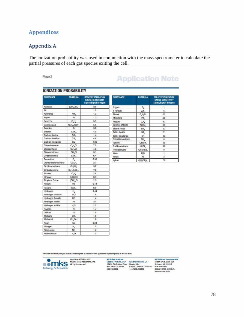
The fuel cell exit gas was passed through the MS and the partial pressure of each species was
recorded within mks’s Process Eye Professional software. The raw values recorded did not
consider the ionization probability of each species, so all of the partial pressure values were
further divided by their respective ionization probabilities as shown in Appendix A. After this
calculation, the mole fraction of the species was able to be calculated based on the new scaled
total pressure. To verify the calibration of the MS data thus acquired, a calibration curve was
generated by feeding a series of CO/H2 blends at known concentrations through the MS. All the
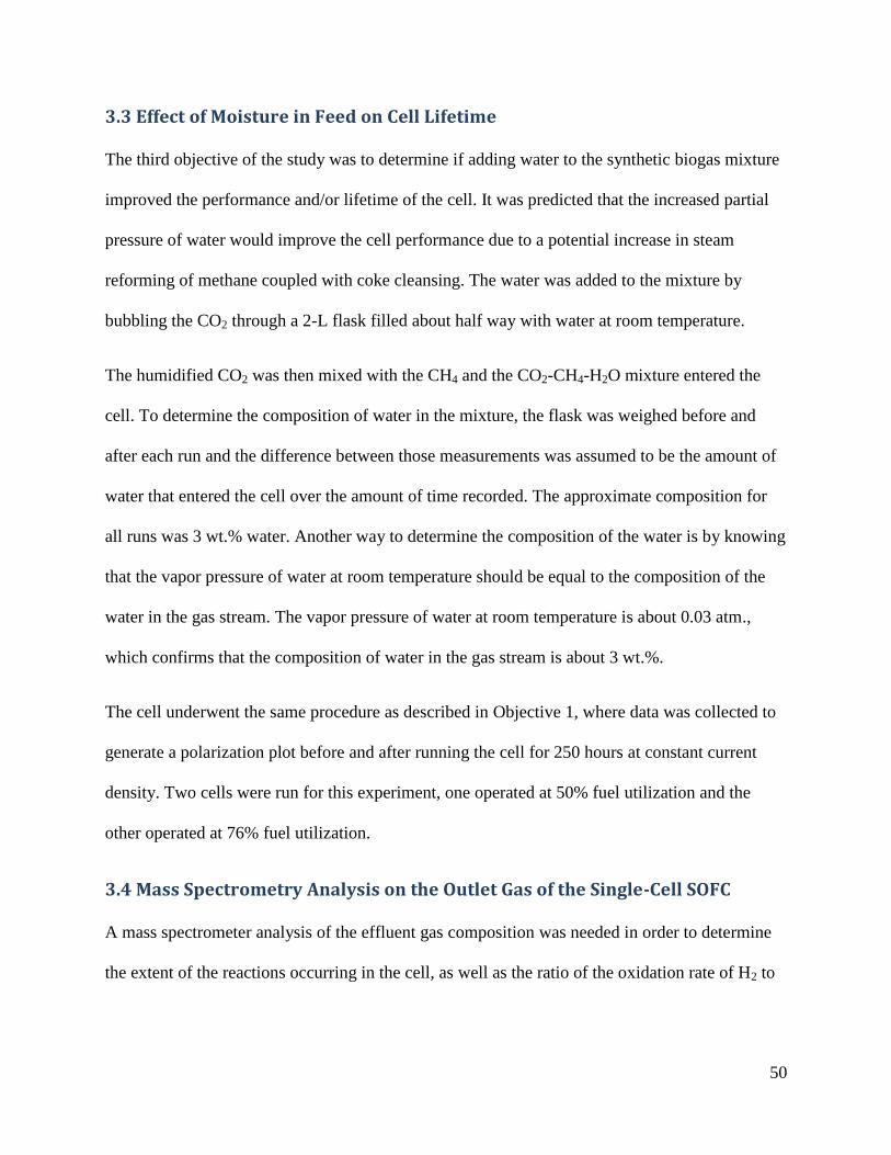
data obtained in this objective was fit to this calibration curve (Figure 26).
Page 52
52
Figure 26: H2 and CO MS calibration curve.
The MS was operated while a cell was running on 45:55 CH4:CO2 at OCV at 900°C in order to
determine the extent of the DR and RWGS reactions (Equation 15). The cell was reduced under
hydrogen conditions as explained in section 3.1, and then converted over to the CH4 and CO2
blend. The cell was held at OCV under these conditions for 30 minutes to obtain steady data for
the equilibrium concentrations of the species.
As the current increased, the H2 and CO were both oxidized to form H2O and CO2. To examine
the relationship between the species during oxidation, the MS was used to measure the
composition of each species at incremental current values. The cell load was held constant for 5
minutes at each current value to ensure equilibrium. The mole fractions of the species were
plotted against current to observe the reactions occurring during oxidation.
Page 53
53
3.4 Effects of 45:55 CH4:CO2 Fuel Through a 5-Cell SOFC Assembly
In addition to the single-cell testing, one test bay was retrofitted to run a pre-made 5-cell T-
SOFC assembly (Figure 27).
Figure 27: 5-Cell T-SOFC Assembly.
With a 5-cell stack, the total fuel flow rate through the cell was 1 SLPM. This flow rate was
consistent with the single-cell flow rate (0.2 SLPM x 5 cells = 1 SLPM). To maintain the 45:55
CH4:CO2 ratio with a total flow rate of 1 SLPM, the flow rates of CH4 and CO2 were 0.45 SLPM
and 0.55 SLPM, respectively. The reducing procedure for the cells was similar to that for the
single-cell test (section 2.1), however, the cells were reduced at 700°C instead of 900°C to
prevent the interconnects from melting while reducing the cells at OCV for 3 hours. Following
the reduction, a polarization plot was generated for the stack running under hydrogen. After that,
the temperature was brought up to 900°C and the fuel was changed from hydrogen to the 45:55
CH4:CO2 mixture. Shortly after, a polarization plot was generated for the stack running on the
Page 54
54
synthetic biogas mixture, and then, to obtain lifetime information for the stack, it was allowed to
run for as long as it could before breaking, which turned out to be about 35 hours.
Page 55
55
4. Results and Discussion
4.1 Effect of Biogas Composition on SOFC Performance
The first objective was to determine how the composition of biogas affects the performance of
the SOFC. Five different CH4:CO2 ratios were tested in addition to pure H2 and CO. Figure 28
shows polarization curves for H2 and CO at 900°C. Figure 29 shows polarization curves for all
five biogas ratios, and for pure H2 and CO all at 900°C. For the experiments with biogas, the
total fuel flow (CO2 and CH4) through the cell was 0.2 SLPM with air flowing over the cathode
at 2 SLPM. For the experiment with H2 and CO, the fuel flow was set at 0.2 SLPM with air
flowing over the cathode at 2 SLPM.
Figure 28: Polarization curve for H2 and CO at 900°C.
Page 56
56
Figure 28: Polarization curves for 5 CH4:CO2 ratios and pure H2 and CO.
According to Figure 29 there is a trend in the open circuit voltage (OCV) with respect to
CH4:CO2 ratio. In general, the greater CH4:CO2 ratio, the greater the OCV (shown in Figure 30).
Page 57
57
Figure 29: OCV Values for various CH4:CO2 ratios.
The lifetime of a cell running on each CH4:CO2 ratio was tested by drawing constant current
density for 150 hours for each test (Figure 31). As predicted by the thermodynamic and Gibbs
free energy calculations, steady state operation at 700°C was not feasible due to short lifetime
(~20 minutes) (Figure 30). For this experiment at 700°C, voltage was held constant at 0.7 V and
the composition entering the cell was similar to that of actual biogas at 60:40 CH4:CO2.
Page 58
58
Figure 30: Lifetime plot for 60:40 CH4:CO2 at 700°C and 0.7 V.
As expected based on the polarization curve, the greater CH4:CO2 ratio, the greater the initial
power density, however, the rates of degradation for 55:45 and 50:50 CH4:CO2 ratios were
greater than those for the 45:55 and 40:60 CH4:CO2 ratios. Table 3 shows the degradation slopes
for each composition as well as the amount of time it would take for each cell to degrade by
10%.
Page 59
59
Figure 31: Lifetime plots for 4 CH4:CO2 ratios.
Table 3: Lifetime data for 4 CH4:CO2 ratios.
CH4:CO2 Ratio Slope 10% Lifetime (h)
40:60 -0.0061 79
45:55 -0.0012 4797
50:50 -0.0069 103
55:45 -0.015 51
As shown by the noise in Figure 31, the performance of the 50:50 and 55:45 CH4:CO2 ratios was
poor after about 30 hours, but the initial power was the highest for the 50:50 and 55:45 CH4:CO2
ratios. The 45:55 CH4:CO2 ratio shows more stable operation than the higher ratios, but the
initial power is lower. Somewhat unexpectedly, the 40:60 CH4:CO2 ratio also shows a steep
degradation slope, and a fair amount of noise after about 40 hours of operation.
0 50 100 1500
1
2
3
4
5
6
7
8
9
10
Time (h)
Po
wer
(W)
40:60 CH4:CO
2
45:55 CH4:CO
2
50:50 CH4:CO
2
55:45 CH4:CO
2
Page 60
60
Table 3 shows the degradation slopes of each ratio, as well as the amount of time before the cell
would degrade by 10%, a number indicative of the point at which there would be operational
difficulties with a system. Although the 45:55 CH4:CO2 ratio did not produce the highest power,
it had the smallest degradation slope, and thus, the longest 10% lifetime at almost 5,000 hours.
Despite the high power produced with the 55:45 CH4:CO2 ratio, this ratio showed the largest
degradation slope, and thus the shortest 10% lifetime at only 50 hours.
As shown in Figure 29, the performance of pure H2 was better than the performance of pure CO
at 900°C. At the higher CH4:CO2 ratios there is excess CH4 that has not been converted via the
dry reforming reaction, and at lower CH4:CO2 ratios there is excess CO that has not been
converted. When there is excess CH4, the CH4 undergoes pyrolysis producing carbon and
additional H2
CH4 ⇌ C + 2H2 (33)
As explained in section 2.3.1, carbon is detrimental to the performance of the cell. The additional
H2 produced from in this reaction could partly explain the high initial power and short-term
performance of the higher CH4:CO2 ratios, but the carbon produced in the reaction could be the
cause of the short lifetime of the higher CH4:CO2 ratios.
The 40:60 CH4:CO2 ratio has excess CO2, which is likely to produce CO via the water gas shift
reaction
CO2 + H2 ⇌ CO + H2O (34)
According to Figure 29, pure CO does not perform as well as pure H2. Because the CO does not
perform as well as H2, the initial power value for the lower CH4:CO2 ratio (excess CO2 that
forms CO) was lower than those for higher CH4:CO2 ratios (excess CH4 that forms H2). In
Page 61
61
addition, when the CO forms from CO2, there is no carbon formation unlike when CH4
decomposes into carbon and H2. The lack of carbon formation causes a longer lifetime for lower
CH4:CO2 ratios compared to higher CH4:CO2 ratios as shown in Figure 31 and Table 3.
When the CH4:CO2 ratio is almost 1 as with the 45:55 CH4:CO2 ratio, the conversion of both
species via the dry reforming reaction is almost maximized. Unlike the stoichiometric 50:50
CH4:CO2 ratio, the 45:55 CH4:CO2 ratio was superior in ensuring that there was little
unconverted methane left to form coke, as discussed in the thermodynamic analysis discussion in
Chpater 3. Further, it allows some room for mass flow controller calibration error or incomplete
mixing between the species because with the 50:50 CH4:CO2 ratio, any slight excess methane
would result in carbon deposition. On the other hand, slight excess CO2 only reduces power and
does not cause any detrimental coking in the cell.
Typically, biogas that exits a biodigester is not a 50:50 CH4:CO2 mixture, but rather a 60:40
CH4:CO2 mixture. Future research aims to test the effects of adding oxygen and water vapor to a
more typical simulated biogas composition (60:40 CH4:CO2) to reduce the methane composition
entering the cell down toward the desirable 45:55 CH4:CO2 and maintain the higher lifetime.
4.2 Effect of Fuel Utilization on SOFC Lifetime
The second objective was to determine the effect of fuel utilization on the lifetime of the cells.
When varying fuel utilization, the 45:55 CH4:CO2 feed ratio was held constant due to its high
lifetime as explained in 4.1. The fuel utilization was set at 35%, 50%, 63%, 76% and 92% for 5
different cells and each cell was run for 250 hours, unless cell failure occurred earlier. Figure 32
shows how the lifetime of a cell running at each fuel utilization was affected by time.
Page 62
62
Figure 32: Lifetime plots for five different fuel utilizations.
The 35% and 50% utilization curves show noise beginning around 100 hrs and 200 hours,
respectively. Although the exact cause of this noise is unknown, it is predicted that this noise
originates from the presence of coke on the anode, causing inconsistencies with electron transfer
and cracks in the electrolyte. The 63%, 76%, and 92% fuel utilization curves are much more
stable, indicating a lack of coke formation under those conditions. Under the hypothesis that
coke results primarily from any unconverted methane, it could be rationalized that lower
utilization means more unconverted methane leading to more coking and shorter lifetimes. It is
also conceivable that at higher fuel utilizations, there is a higher partial pressure of water in the
reactor, which helps to flush out any coke there is out of the reactor by reacting with the carbon
H2O + C ⇌ CO + H2 (35)
0 100 2504
6
8
10
12
14
16
Time (h)
Po
wer
(W)
7.24 A (35% Uf), slope = -0.0012
10.33 A (50% Uf), slope = -0.002
12.92 A (63% Uf), slope = -0.0018
15.51 A (76% Uf), slope = -0.00039
18.81 A (92% Uf), slope = -0.00022
Page 63
63
The cell running at 76% utilization demonstrated a minimal rate of degradation. Figure 33 shows
the polarization plot for the cell running at 76% fuel utilization before and after the cell ran for
250 hours.
Figure 33: Polarization curve for before and after 250 hours of operation at 76% fuel utilization.
Clearly, there is minimal difference between the two plots, indicating that there was no
significant amount of coking occurring in the cell running at 76% fuel utilization and a 45:55
CH4:CO2 ratio for 250 hours. Thus, higher utilizations are desirable to extend the life of the fuel
cell.
4.3 Effect of Moisture in Feed on Cell Lifetime
The third objective was to determine the effects of water addition in the feed on the lifetime of
the cells. To determine if a humidified feed improved the lifetime of the cell, 4 cells were run for
0 5 10 15 20 250.7
0.75
0.8
0.85
0.9
0.95
1
1.05
1.1
Current (A)
Vo
ltag
e (
V)
0
5
10
15
20
Po
wer
(W)
Before 250 Hours
After 250 Hours
Page 64
64
250 hours at a constant current density and with the 45:55 CH4:CO2 ratio. Two of the cells ran at
15.51 A, which corresponded to 76% Uf humidified and unhumidified, and the other two cells
ran at 10.33 A (50% Uf) humidified and unhumidified. As shown in Figure 34, the water addition
had no effect on the degradation rate of the higher fuel utilization run, but did improve the
degradation rate of the lower utilization run.
Figure 34: Degradation rates for cells running with and without water at different utilizations.
There is little difference between the humidified and unhumidified cells at the higher utilization
and current density. This is likely due to the fact that at this higher utilization and current density
there is less unconverted methane to form coke and there is more water produced via the
oxidation of hydrogen than at the lower current density, so that adding more water to the stream
does not significantly affect the performance of the cell. At the lower utilization and current
density, however, the failure that occurred without water was likely due to coking caused by a
0 50 100 150 200 2500
2
4
6
8
10
12
14
16
Time (h)
Po
wer
(W)
15.51 A (76% Uf)
10.33 A (50% Uf)
Page 65
65
higher level of unconverted methane. The water addition obviously reduced coking and
degradation, as suggested by the more stable operation. An increase in the amount of water in the
cell appears to decreases the risk cell failure due to carbon deposition. This is consistent with the
notion that at lower fuel utilization when there is higher coke formation rate (Figure 32), water
has a beneficial effect on reduced coking via the cleansing reaction indicated in Eq. (35).
4.4 Mass Spectrometry Analysis on the Outlet Gas of the Single-Cell SOFC
The fourth objective was to analyze the outlet gas composition of a single-cell SOFC running on
biogas under different operating conditions. This analysis was performed when the cell running
on 45:55 CH4:CO2 at 900°C was under both OCV and under a load. Figure 35 shows how the
composition of each species changes as the load increases. The cell was held at each current
value for five minutes to ensure steady-state. The changes in mole fraction of each of the species
was expected except for that of methane. A potential reason for the mole fraction of methane
increasing as the load increased is because the gas cooled slightly as it passed through the
capillary tube into the mass spectrometer (the capillary was heated to 100C). This may have
caused the CO2 and H2 to reform CH4 as the amount of CO2 increased.
Page 66
66
Figure 35: Change in composition of species for incremental current values.
When the current was 0, the cell was under OCV, and all reactions (dry reforming and reverse
water gas shift) were presumably at DR and RWGS equilibrium. According to the
thermodynamic analysis presented in section 3.2, the compositions of each species at
OCV/equilibrium are as follows:
𝑥CH4,𝑒 = 0.0086; 𝑥CO2,𝑒 = 0.0207; 𝑥H2O,𝑒 = 0.0415; 𝑥H2,𝑒 = 0.4231; 𝑥CO,𝑒 = 0.5061.
These values are similar to the values shown in Figure 35 at OCV, but they are not identical. For
example, the measured CO mole fraction is about 0.02 less than the theoretical, and the measured
CO2 and H2O mole fractions are about 0.03 more than the theoretical. For the theoretical
analysis, the enthalpy of the reactions (∆𝐻𝑂𝑅𝑜 ) was assumed to be constant with temperature,
which could explain the difference between theoretical and measured OCV/equilibrium values
because in reality, the enthalpy is a function of temperature.
Page 67
67
∆𝐻𝑇0 = ∆𝐻298
0 + ∫ ∆𝐶𝑝𝑑𝑇𝑇
𝑇298
(36)
The Gibbs free energy of the methane decomposition and the Boudouard reactions are provided
as functions of temperature in equations 37 and 38 below, respectively (Ginsburg et al., 2005).
∆G𝑜 = 58886.79 + 270.55𝑇 + 0.0311𝑇2 − (3.00 × 10⁻⁶)𝑇3 +291405.7
𝑇
− 54.598𝑇 ln(𝑇)
(37)
∆G𝑜 = −188030.19 + 402.82𝑇 + 0.00524𝑇2 +828509.9
𝑇− 32.026𝑇 ln(𝑇)
(38)
As discussed in Chapter 2 and shown in Figure 36, the oxidation of both H2 and CO generate
power. Due to the slightly larger rate of oxidation of H2 than CO, the total power generated
comes slightly more from H2 than CO.
Page 68
68
Figure 36: H2 and CO composition and respective and total power generation for incremental current
values.
The MS was calibrated before running the experiment, however, there are many factors in the
testing apparatus that could cause errors. Due to this concern, all H2 and CO mole fractions
obtained in the MS analysis were fitted to the calibration curve shown in Figure 26.
4.5 Effects of 45:55 CH4:CO2 Fuel Through a 5-Cell SOFC Assembly
The fifth objective was to operate a 5-cell SOFC stack on the biogas conditions proven to be
successful thus far. These conditions were 45:55 CH4:CO2 and 76% fuel utilization at 900°C.
Figure 37 shows a polarization curve for the 5-cell stack running on these conditions.
Page 69
69
Figure 37: Polarization curve for 5-cell stack on biogas.
As shown in Figure 37, the 5-cell stack achieved a power of about 52 watts. If there were no
losses throughout the stack, the power simply be the product of the number of cells and the
power each cell produces. If, according to previous results (Figure 32), each cell is assumed to
produce 12 watts, a 5-cell stack with no additional losses would produce a power of 60 watts.
The slightly lower power produced in the stack is reasonable, and indicates that scaling up this
SOFC system fed by biogas to eventually become a larger-scale, commercialized unit is entirely
feasible.
Page 70
70
5. Conclusions and Commercialization Potential
5.1 Conclusions
When looking at the results of the single-cell and 5-cell testing, it is clear that synthetic biogas
can be fed through an SOFC to generate electricity. The most successful operating conditions
were an operating temperature of 900ºC, a biogas composition of 45:55 CH4:CO2 and a high fuel
utilization, at or above 76%. Under these conditions, the cell produced high power (12 watts per
cell), and demonstrated long lifetime (estimated as about 7,000 hours before 10% degradation). It
was also observed that adding water to the feed improved the lifetime of the SOFC operating at a
low fuel utilization (50%). The mass spectrometer analysis confirmed the theoretical
thermodynamic analysis due to the species’ concentrations shown at OCV, and the relationship
between the H2 and CO concentrations and the current being drawn. The scaled-up 5-cell stack
operating under 45:55 CH4:CO2 and 900°C achieved a power of about 52 watts, suggesting that
scaled-up units for practical applications have potential.
Based on the results obtained in this study, a 25-cell SOFC stack running on biogas under the
conditions specified above has the potential to produce about 200 watts assuming the stack
would experience about 30% losses. If the lifetime of the system was assumed to be about
10,000 hours, the energy rating for a 25-cell SOFC stack running on biogas would be 2,000
kWh.
5.2 Commercialization Potential
As discussed in Section 2.2, biogas infrastructure is readily available in many rural and
developing countries around the world, and is currently used for cooking and heating. An SOFC
would utilize the current infrastructure, but also introduce a clean and convenient way to
Page 71
71
generate electricity. A small school in a village in Chhattisgarh, India uses about 465 kWh of
electricity per year (Sen and Bhattacharyya, 2014). If the 2,000 kWh 25-cell biogas SOFC were
to be utilized by the school, there are three implementation scenarios that have potential to be
successful.
The first scenario would be to utilize solely the SOFC system. This would be the simplest model,
as it capitalizes on the current infrastructure available, biogas. For this model, the SOFC would
run constantly on about 7.5 m3 of biogas per day until the point at which cell degradation causes
poor SOFC performance. According to the results from this study, and assuming a maximum
constant load of 54 watts for 10,000 hours, this would allow for a 14-18 month lifetime of the
system. On average, this would generate a constant power supply to provide adequate electricity
for the school’s current needs for 14-18 months.
The second scenario would be to create an SOFC-battery hybrid system. Adding the battery to
the system would allow for the energy produced in the SOFC to be stored in the battery for later
use, allowing it to run under steady conditions despite varying demand during the day. Storing
the energy could extend the lifetime of the SOFC to be longer than 14-18 months because it
would be operating at a lower power density under stable conditions than under varying
conditions throughout the day as the demand varies. If the school uses 465 kWh per year, the
daily energy consumption is 1.6 kWh per day. The SOFC would thus only need to run for 6.5
hours each day to generate this much electricity. After the SOFC runs for 6.5 hours, it could be
turned off until the battery needs recharging. This model could extend the lifetime of the SOFC
to be about 4 years. However, in reality, there is a tradeoff between lifetime and cycling, which
generally leads to faster degradation. With the SOFC being turned on and off every time the
battery needs recharging, there is a great deal of mechanical stress on the cells and the system.
Page 72
72
This would potentially require the SOFC to undergo cycling maintenance every 500 hours or so,
but the overall lifetime of the SOFC in an SOFC-battery hybrid system could be greater than that
of solely an SOFC system. On the other hand, an alternate way to extend the life is for the cell to
operate steadily under a lower load, or alternately the cost of the unit could be decreased by
utilizing a smaller unit.
The third scenario would be to implement a solar-SOFC-battery hybrid system. This system
would first utilize a solar panel when the conditions are appropriate (i.e., sunlight), and then,
when the conditions are not ideal for the solar panel, the system would tap into the energy stored
in the battery from the SOFC. The SOFC-battery system would be similar to that explained
above in that the SOFC would run for about 6.5 hours per day to charge the battery, but because
the solar panel is also present and assumed to be utilizable 25% of the uptime of the school, the
SOFC lifetime now extends to about 5 years. Alternately, again a smaller SOFC unit would
suffice.
An economic analysis for each scenario would be needed to determine the most cost effective
way to balance the lifetime and cycling maintenance of the SOFC with the capital, operational,
and total costs. On the consumer end, if the system were to be large enough, a utility model
where a community or non-governmental organization rents or purchases the system at a fixed
cost would allow residents to pay a marginal amount for a clean form of electricity.
5.3 Recommendations for Future Work
The next step in the work would be to obtain actual biogas samples from a local digester. These
samples could be analyzed to determine their gas composition, and then fed through a sulfur
filter to filter out the H2S and any other impurities that could harm the SOFC. If the composition
Page 73
73
of water in the sample is not significant, water could be added to the sample to improve the
lifetime, as shown in Figure 34 above.
To potentially decrease the cost associated with a 25-cell stack system, the biogas could be
heated to 900°C externally, allowing the SOFC itself to run on the H2 and CO at 700°C instead
of 900°C. This process could be designed and tested with single cells to determine its feasibility
compared to operating the SOFC at 900°C.
More scale-up testing could be completed with synthetic biogas. Lifetime data could be obtained
with the 5-cell stack, especially a fuel utilization and water addition versus lifetime matrix,
similar to the single-cell tests explained in sections 4.2 and 4.3. Once operating conditions are
optimized for synthetic biogas in the 5-cell stack, actual biogas samples could be tested in the 5-
cell stack with the sulfur filter. A 25-cell stack could then be tested with both synthetic biogas
and an actual biogas sample to provide data for a unit with potential for commercialization.
Page 74
74
References
Anaerobic Digestion. Renewable Energy Concepts. Retrieved 23 March 2016, from
http://www.renewable-energy-concepts.com/biomass-bioenergy/biogas-basics/anaerobic-
digestion.html
Assabumrungrat, S., Laosiripojana, N., & Piroonlerkgul, P(2006). Determination of the boundary
of carbon formation for dry reforming of methane in a solid oxide fuel cell, 159, 1274–
1282. http://doi.org/10.1016/j.jpowsour.2005.12.010
Baker, R., & Zhang, J(2011). Proton Exchange Membrane or Polymer Electrolyte Membrane
(PEM) Fuel Cells. The Electrochemical Society. Retrieved 23 March 2016, from
http://knowledge.electrochem.org/encycl/art-f04-fuel-cells-pem.htm
Biogas Composition. Renewable Energy Concepts. Retrieved 23 March 2016, from
http://www.renewable-energy-concepts.com/biomass-bioenergy/biogas-basics/gas-
composition.html
Bond, T., & Templeton, M. R(2011). History and future of domestic biogas plants in the
developing world. Energy for Sustainable Development, 15(4), 347–354.
http://doi.org/10.1016/j.esd.2011.09.003
Carlowicz, M. World of Change: Global Temperatures. NASA Earth Observatory. Retrieved 22
May 2015, from
http://earthobservatory.nasa.gov/Features/WorldOfChange/decadaltemp.php
Cropgen,. Renewable energy from crops and agrowastes. Retrieved 1 June 2015, from
http://www.cropgen.soton.ac.uk/deliverables.htm
El-Mashad, H. M., & Zhang, R. (2010). Biogas production from co-digestion of dairy manure
and food waste. Bioresource Technology, 101(11), 4027.
http://doi.org/10.1016/j.biortech.2010.01.027
EPA,. Methane Emissions. Retrieved 25 May 2015, from
http://epa.gov/climatechange/ghgemissions/gases/ch4.html
FAO,. Energy in the World Economy. Retrieved 22 May 2015, from
http://www.fao.org/docrep/003/x8054e/x8054e04.htm
Fehrenbacher, K(2013). Apple now powering its cloud with solar panels, fuel cells (photos).
Gigaom. Retrieved 23 March 2016, from https://gigaom.com/2013/03/21/apple-now-
powering-its-cloud-with-solar-panels-fuel-cells-photos/
Fitzsimmons, A(2013). The Bloom is Off Bloom Energy. Institute for Energy Research.
Retrieved 23 March 2016, from http://instituteforenergyresearch.org/analysis/the-bloom-
is-off-bloom-energy/
Page 75
75
Fogler, H., Aguilar Ortega, M., & Ramirez Lopez, R. (2008). Elementos de ingenieria de las
reacciones quimicas. Naucalpan de Juarez, Mexico.: Pearson Educacion.
Fuel Cell Energy,. How do Fuel Cells Work?. Retrieved 25 May 2015, from
http://www.fuelcellenergy.com/why-fuelcell-energy/how-do-fuel-cells-work/
Fuel Cell Technology Market by Types(2014). Markets and Markets. Retrieved 24 March 2016,
from http://www.marketsandmarkets.com/Market-Reports/fuel-cell-market-348.html
Garrison, E. Solid Oxide Fuel Cells. IIT. Retrieved 25 May 2015, from
http://mypages.iit.edu/~smart/garrear/fuelcells.htm
Ginsburg, J. M., Piña, J., El Solh, T., & De Lasa, H. I. (2005). Coke formation over a nickel
catalyst under methane dry reforming conditions: Thermodynamic and kinetic models.
Industrial & engineering chemistry research, 44(14), 4846-4854
Goodwin, D. G., Zhu, H., Colclasure, A. M., and Kee, R. J. “Modeling Electrochemical
Oxidation of Hydrogen on Ni-YSZ Pattern Anodes,” J. Electrochem. Soc., 156, B1004-
B1021 (2009).
Hecht, E. S., Gupta, G. K., Zhu, H., Dean, A. M., Kee, R. J., Maier, L., & Deutschmann,
O(2005). Methane reforming kinetics within a Ni-YSZ SOFC anode support. Applied
Catalysis A: General, 295(1), 40–41. http://doi.org/10.1016/j.apcata.2005.08.003
Homel, M., Gür, T. M., Koh, J. H., & Virkar, A. V. (2010). Carbon monoxide-fueled solid oxide
fuel cell. Journal of Power Sources, 195(19), 6367-6372.
Introduction to Fuel Cell Technology - Overview(2012). NPTEL. Retrieved 23 March 2016, from
http://www.nptel.ac.in/courses/103102015/2
Janardhanan, V. & Deutschmann, O. (2007). Modeling of Solid-Oxide Fuel Cells. Zeitschrift Für
Physikalische Chemie, 221(4), 443-478. http://dx.doi.org/10.1524/zpch.2007.221.4.443
Lanzini, A., Leone, P., Guerra, C., Smeacetto, F., Brandon, N. P., & Santarelli, M(2013).
Durability of anode supported Solid Oxides Fuel Cells (SOFC) under direct dry-
reforming of methane. Chemical Engineering Journal, 220, 254–263.
http://doi.org/10.1016/j.cej.2013.01.003
Laosiripojana, N., & Assabumrungrat, S(2007). Catalytic steam reforming of methane, methanol,
and ethanol over Ni/YSZ: The possible use of these fuels in internal reforming SOFC.
Journal of Power Sources, 163(2), 943–951.
http://doi.org/10.1016/j.jpowsour.2006.10.006
Mebarki, B., Adouane, B., Khaldi, F., Dehimi, S., & Haddad, D(2015). ScienceDirect
Theoretical estimation of the production of biogas from the landfill of Batna city and its
electrical conversion by a SOFC. International Journal of Hydrogen Energy, 40(39),
13799–13805. http://doi.org/10.1016/j.ijhydene.2015.03.062
Page 76
76
Mermelstein, J., Millan, M., & Brandon, N. P(2011). The interaction of biomass gasification
syngas components with tar in a solid oxide fuel cell and operational conditions to
mitigate carbon deposition on nickel-gadolinium doped ceria anodes. Journal of Power
Sources, 196(11), 5027–5034. http://doi.org/10.1016/j.jpowsour.2011.02.011
Muzenda, E(2014). Bio-methane Generation from Organic Waste : A Review, II, 4.
Olivier, M(2008). Fuel Cell Characterization. Presentation, Academie Universitaire Wallonie-
Bruxelles.
Papadam, T., Goula, G., & Yentekakis, I. V(2012). Long-term operation stability tests of
intermediate and high temperature Ni-based anodes’ SOFCs directly fueled with
simulated biogas mixtures. International Journal of Hydrogen Energy, 37(21), 16680–
16685. http://doi.org/10.1016/j.ijhydene.2012.02.147
Population Reference Bureau,. Human Population: Population Growth. Retrieved 3 June 2015,
from http://www.prb.org/Publications/Lesson-
Plans/HumanPopulation/PopulationGrowth.aspx
Protonex,. Solid Oxide Fuel Cell Technology. Retrieved 25 May 2015, from
http://www.protonex.com/technology/solid-oxide-fuel-cell/
Rayment, C(2003). Introduction to Fuel Cell Technology, 19–38. http://doi.org/10.1.1.129.3231
SAE International., (2015). Fuel Cell Technology Showcase - History of Fuel Cells. Retrieved 10
June 2015, from http://www.sae.org/fuelcells/fuelcells-history.htm
Sen, R. & Bhattacharyya, S. (2014). Off-grid electricity generation with renewable energy
technologies in India: An application of HOMER. Renewable Energy, 62, 388-398.
http://dx.doi.org/10.1016/j.renene.2013.07.028
Services of SRC’s Wastewater Treatment Unit(2012). Scientific Research Council. Retrieved 22
March 2016, from http://www.src.gov.jm/services-wastewater-treatment-unit/
Shiratori, Y., Ijichi, T., Oshima, T., & Sasaki, K(2010). Internal reforming SOFC running on
biogas. International Journal of Hydrogen Energy, 35(15), 7905–7912.
http://doi.org/10.1016/j.ijhydene.2010.05.064
Standardization in SOFC Testing. Fuel Cell Markets. Retrieved 23 March 2016, from
http://www.fuelcellmarkets.com/content/images/articles/WP1.pdf
Taherzadeh, Mohammad. "Waste Biorefinery: Biogas In Vietnam". University of Boras. N.p.,
2012. Web. 23 Mar. 2016.
Technologies(2016). Fuel Cell Today. Retrieved 23 March 2016, from
http://www.fuelcelltoday.com/technologies
Page 77
77
The Biodigester and its Benefits(2014). TransformAsia. Retrieved 22 March 2016, from
http://www.transformasia.us/biodigester-and-it-benefits/
Tubular SOFC, Solid Oxide Fuel Cell Technology. Acumentrics. Retrieved 23 March 2016, from
http://www.acumentrics.com/sofc-products-fuel-cell-technology.htm
U.S. Department of Energy, Office of Fossil Energy, (2004). Fuel Cell Handbook (pp. 2-12).
Morgantown, West Virginia.
Vindis, P., & Mursec, B(2009). The impact of mesophilic and thermophilic anaerobic digestion
on biogas production. Journal of Achievements …, 36(2), 197. Retrieved from
http://ww.journalamme.org/papers_vol36_2/36210.pdf
Waldemar Bujalski, Chinnan M. Dikwal, Kevin Kendall, “Cycling of three solid oxide fuel cell
types,” Journal of Power Sources, Volume 171, Issue 1, 19 September 2007, Pages 96-
100.
Wang, Y., Chen, K. S., Mishler, J., Cho, S. C., & Adroher, X. C(2011). A review of polymer
electrolyte membrane fuel cells: Technology, applications, and needs on fundamental
research. Applied Energy, 88(4), 981–1007.
http://doi.org/10.1016/j.apenergy.2010.09.030
Yi, Y., Rao, A. D., Brouwer, J., & Samuelsen, G. S(2005). Fuel flexibility study of an
integrated 25 kW SOFC reformer system. Journal of Power Sources, 144(1), 1.
http://doi.org/10.1016/j.jpowsour.2004.11.068
Page 78
78
Appendices
Appendix A
The ionization probability was used in conjunction with the mass spectrometer to calculate the
partial pressures of each gas species exiting the cell.
Page 79
79
Appendix B
A procedure was written into the Universal Data Acquisition (UDA) Software as shown below.
Page 84
84
Appendix C
The standard enthalpy and entropy values for each of the species analyzed in this work were
gathered from the table below.