69

Performance Trends of a Large Air-Cooled Steam
Condenser during Windy Conditions
by
Francois G. Louw
Thesis presented in partial ful�lment of the requirements forthe degree of Master of Science in Engineering (Mechanical)
at Stellenbosch University
Department of Mechanical and Mechatronic Engineering,University of Stellenbosch,
Private Bag X1, Matieland 7602, South Africa.
Supervisor: Prof. D.G. Kröger
March 2011
Declaration
By submitting this thesis electronically, I declare that the entirety of the workcontained therein is my own, original work, that I am the owner of the copy-right thereof (unless to the extent explicitly otherwise stated) and that I havenot previously in its entirety or in part submitted it for obtaining any quali�-cation.
Date: . . . . . . . . . . . . . . . . . . . . . . . . . . . . . . .
Copyright© 2011 Stellenbosch UniversityAll rights reserved.
i
Abstract
Performance Trends of a Large Air-Cooled SteamCondenser during Windy Conditions
F.G. Louw
Department of Mechanical and Mechatronic Engineering,
University of Stellenbosch,
Private Bag X1, Matieland 7602, South Africa.
Thesis: MScEng (Mech)
March 2011
Large air-cooled steam condensers (ACSC's) �nd application in power stationsand utilize arrays of large fans and heat-exchanger bundles to condense steamwith a forced draft of ambient air. A numerical investigation was conductedin an attempt to extend knowledge on the �ow distribution in the vicinity of alarge ACSC (consisting of 384 fans) during windy periods. A three-dimensionalnumerical model of a large ACSC was subjected to various wind speeds in across and longitudinal direction (wind perpendicular and parallel to the longestside of the ACSC respectively). The study revealed that the �ow approach-ing the ACSC could be classi�ed as two- and three-dimensional depending onthe in�ow location of the ACSC. Fan performance is adversely a�ected due toseparation at the upstream edge of the fan platform and is the worst in thetwo-dimensional �ow area. Recirculation of hot plume was observed on thesides of the ACSC, parallel to the wind direction, as well as on the upstreamperiphery. Recirculation on the upstream edge increased in areas where the�ow is two-dimensional. The study showed that a signi�cant reduction inACSC e�ectiveness occurs due to cross winds, whereas an overall e�ectivenessincrease is seen for longitudinal winds. The e�ect of power station buildingplacement on overall ACSC performance was also investigated. During windyconditions, fan performance mainly contributed to the reduction in ACSC per-formance, except for the cross-wind case where the wind blows from behindthe boiler houses and turbine hall onto the ACSC. Wind mitigation measuresin the form of di�erent skirt and screen con�gurations were implemented onthe Large ACSC, in an attempt to improve overall fan performance and re-duce recirculation. The e�ect of individual skirts, screens and combinations of
ii

ABSTRACT iii
these were investigated. Skirt widths provided an ACSC performance increasebetween 2-9%. A considerably greater improvement in ACSC performance,ranging from 8-30%, was achieved by means of screens. It is recommendedthat a further investigation be conducted to draw conclusions regarding thee�ect of various distances between the power station buildings and the ACSCon overall ACSC e�ectiveness. The orientation of the ACSC, regarding thedominant wind direction, should also be reconsidered in any future design.

Uittreksel
Tendense in die Verkoelingsvermoë van 'n GrootLugverkoelde Stoom Kondensor gedurende Winderige
Toestande
(�Performance Trends of a Large Air-Cooled Steam Condenser during Windy
Conditions�)
F.G. Louw
Departement Meganiese en Megatroniese Ingenieurswese,
Universiteit van Stellenbosch,
Privaatsak X1, Matieland 7602, Suid Afrika.
Tesis: MScIng (Meg)
Maart 2011
Groot lugverkoelde stoom kondensors (LVSK's) word gebruik in kragstasiesen bestaan uit rangskikkings van groot waaiers en vin-buis bundels om stoomte kondenseer deur middel van atmosferiese lug. 'n Numeriesie ondersoekwas geloods in 'n poging om huidige kennis behelsende die vloeiverdeling indie nabyheid van 'n groot LVSK (wat bestaan uit 384 waaiers) te ondersoekgedurende winderige atmosferiese toestande. 'n Drie-dimensionele numeriesemodel van die groot LVSK was ondersoek deur die stelsel te belas met verskil-lende windsnelhede vanuit 'n kruis en langs rigting (wind loodreg en parallelaan die langste sy van die kondensor onderskeidelik). Die studie het twee- endrie-dimensionele vloei areas uitgewys, afhangend van die gebied waar die luginvloei. Waaiervermoë neem af as gevolg van wegbreking by die stroom-oprand van die LVSK en is die laagste vir die waaiers in die twee-dimensionelevloeigebied. Hersirkulasie van warm pluim lug was waargeneem by die kante,parallel aan die windrigting, asook rondom die stroom-op rand. 'n Toenamein die stroom-op hersirkulasie was ook waargeneem namate die vloei twee-dimensioneel raak. Die e�ek van die kragstasiegeboue op die e�ektiwiteit vandie LVSK was ook ondersoek. Die studie het gewys dat waaiervermoë diegrootste bydrae maak tot die afname in die groot LVSK se e�ektiwiteit, be-halwe in die geval waar die wind van agter die kragstasie geboue op die LVSKwaai. In 'n poging om die afname in die LVSK se e�ektiwiteit teen te werk wasverskillende loopvlakke en skerms op en rondom die LVSK aangebring. Die
iv

UITTREKSEL v
e�ek van individuele loopvlakke, skerms asook 'n kombinasie van hierdie wasondersoek. Loopvlakke het oor die algemeen 'n verbetering tussen 2 en 9 %aangebring in die e�ektiwiteit van die LVSK, maar 'n groter verbetering wasveroorsaak deur die implimentering van skerms wat in die orde van tussen 8en 30 % was. Dit word voorgestel dat 'n verdere ondersoek geloods moet wordom die e�ek van verskillende afstande tussen die gebou en die LVSK op diealgemene e�ektiwiteit van die LVSK te bepaal. Die konvensionele oriëntasievan groot LVSK's moet ook heroorweeg word vir dominante windrigtings indie toekomstige ontwerp van groot LVSK's.

Acknowledgements
My acknowledgments go to the Lord, Jesus Christ, in whom I found salvationand is constantly teaching me truth, whether about life, people or engineering.I experience His smile throughout my life.
To professor Detlev G. Kröger who provided excellent guidance to this re-search. I will always remember the additional wisdom and laughter he addedin the many meetings we had.
To my parents Irma and Johan, friends parents, many mentors, the multi-tude of friends surrounding me (whose names are too many) and my girlfriendJeanne, for their aid through the tough times and their praise through thegood times of this project. Each one of the mentioned is as close as family andthe constant encouragement by them is/was appreciated incredibly.
To ESKOM for the funding and information applicable to this project.
To Q�nsoft and ANSYS for the provision of academic CFD software li-censes and support.
To the sta� of the Mechanical and Mechatronic Engineering Department,University of Stellenbosch and other departments of the university for all theadministration, the provision of high performance computational facilities andconstant help.
vi

Dedications
To my family and friends
vii
Contents
Declaration i
Abstract ii
Uittreksel iv
Contents viii
List of Figures xii
List of Tables xvi
Nomenclature xvii
1 Introduction 11.1 Background . . . . . . . . . . . . . . . . . . . . . . . . . . . . . 11.2 Literature survey . . . . . . . . . . . . . . . . . . . . . . . . . . 51.3 Research objective . . . . . . . . . . . . . . . . . . . . . . . . . 11
2 ACSC system description 142.1 Applicable system details . . . . . . . . . . . . . . . . . . . . . . 14
2.1.1 Van Rooyen (2007) ACSC . . . . . . . . . . . . . . . . . 142.1.2 Large ACSC . . . . . . . . . . . . . . . . . . . . . . . . . 16
2.2 System components . . . . . . . . . . . . . . . . . . . . . . . . . 162.2.1 Axial fan . . . . . . . . . . . . . . . . . . . . . . . . . . . 162.2.2 Heat-exchanger bundles . . . . . . . . . . . . . . . . . . 17
2.3 Flow and heat transfer analysis . . . . . . . . . . . . . . . . . . 182.3.1 Flow calculation . . . . . . . . . . . . . . . . . . . . . . . 182.3.2 Heat transfer calculation . . . . . . . . . . . . . . . . . . 19
3 Numerical modeling 203.1 CFD code summary . . . . . . . . . . . . . . . . . . . . . . . . . 21
3.1.1 Governing equations . . . . . . . . . . . . . . . . . . . . 213.1.2 Discretization and solver settings . . . . . . . . . . . . . 233.1.3 Turbulence modeling . . . . . . . . . . . . . . . . . . . . 24
viii

CONTENTS ix
3.1.4 Buoyancy modeling . . . . . . . . . . . . . . . . . . . . . 243.1.5 Boundary conditions . . . . . . . . . . . . . . . . . . . . 25
3.2 Modeling of a single fan unit . . . . . . . . . . . . . . . . . . . . 263.2.1 Heat-exchanger model . . . . . . . . . . . . . . . . . . . 273.2.2 Fan model . . . . . . . . . . . . . . . . . . . . . . . . . . 293.2.3 Single fan-unit grid . . . . . . . . . . . . . . . . . . . . . 30
3.3 Modeling procedures . . . . . . . . . . . . . . . . . . . . . . . . 323.3.1 Modeling of wind . . . . . . . . . . . . . . . . . . . . . . 323.3.2 Modeling procedure for the Van Rooyen (2007) ACSC . . 333.3.3 Iterative modeling procedure for the Large ACSC . . . . 34
3.4 Presentation of performance results . . . . . . . . . . . . . . . . 373.4.1 Volumetric e�ectiveness . . . . . . . . . . . . . . . . . . 373.4.2 Heat transfer e�ectiveness . . . . . . . . . . . . . . . . . 38
4 Validation of numerical analysis 394.1 Validation of an independent fan-unit . . . . . . . . . . . . . . . 39
4.1.1 Volumetric �ow rate . . . . . . . . . . . . . . . . . . . . 394.1.2 Heat transfer . . . . . . . . . . . . . . . . . . . . . . . . 40
4.2 Comparison to previous work . . . . . . . . . . . . . . . . . . . 424.3 Sensitivity analysis . . . . . . . . . . . . . . . . . . . . . . . . . 45
4.3.1 Boundary proximity . . . . . . . . . . . . . . . . . . . . 454.3.2 Grid density . . . . . . . . . . . . . . . . . . . . . . . . . 46
4.4 Convergence . . . . . . . . . . . . . . . . . . . . . . . . . . . . . 464.4.1 Convergence of a single simulation . . . . . . . . . . . . 464.4.2 Convergence of subsequent simulations . . . . . . . . . . 48
5 ACSC performance during windy conditions 495.1 Overall heat-transfer e�ectiveness of the Large ACSC . . . . . . 495.2 Reduced fan performance . . . . . . . . . . . . . . . . . . . . . . 51
5.2.1 𝑥-direction winds . . . . . . . . . . . . . . . . . . . . . . 515.2.2 𝑦-direction winds . . . . . . . . . . . . . . . . . . . . . . 53
5.3 Plume recirculation . . . . . . . . . . . . . . . . . . . . . . . . . 565.3.1 𝑥-direction wind . . . . . . . . . . . . . . . . . . . . . . . 565.3.2 𝑦-direction wind . . . . . . . . . . . . . . . . . . . . . . . 57
5.4 Comparison between the e�ect of fan performance and plumerecirculation on overall ACSC performance . . . . . . . . . . . . 595.4.1 𝑥-direction wind . . . . . . . . . . . . . . . . . . . . . . . 605.4.2 𝑦-direction wind . . . . . . . . . . . . . . . . . . . . . . . 605.4.3 Conclusion . . . . . . . . . . . . . . . . . . . . . . . . . . 62
5.5 E�ect of main power plant buildings . . . . . . . . . . . . . . . 625.5.1 Positive 𝑥-direction wind . . . . . . . . . . . . . . . . . . 625.5.2 Negative 𝑥-direction wind . . . . . . . . . . . . . . . . . 64
6 Evaluation of ACSC wind mitigation modi�cations 68

CONTENTS x
6.1 E�ect of skirts . . . . . . . . . . . . . . . . . . . . . . . . . . . . 686.2 E�ect of screens and de�ection walls . . . . . . . . . . . . . . . 716.3 Combined e�ect of skirts and screens . . . . . . . . . . . . . . . 74
6.3.1 Case 1 . . . . . . . . . . . . . . . . . . . . . . . . . . . . 746.3.2 Case 2 . . . . . . . . . . . . . . . . . . . . . . . . . . . . 756.3.3 Case 3 . . . . . . . . . . . . . . . . . . . . . . . . . . . . 75
7 Conclusion 777.1 Performance trends of the Large ACSC under wind . . . . . . . 77
7.1.1 Positive x-direction wind . . . . . . . . . . . . . . . . . . 777.1.2 Positive y-direction wind . . . . . . . . . . . . . . . . . . 78
7.2 E�ect of power station buildings and wind mitigation measures . 797.2.1 E�ect of power station buildings . . . . . . . . . . . . . . 797.2.2 E�ect of skirts . . . . . . . . . . . . . . . . . . . . . . . . 807.2.3 E�ect of screens and de�ection wall . . . . . . . . . . . . 807.2.4 E�ect of skirt-screen combinations . . . . . . . . . . . . 80
7.3 Further research . . . . . . . . . . . . . . . . . . . . . . . . . . . 81
List of References 83
Appendices 87
A Speci�cations 88A.1 Speci�cations for the Van Rooyen (2007) ACSC . . . . . . . . . 88
A.1.1 Atmospheric and steam design conditions . . . . . . . . . 88A.1.2 Properties of air at the design condition . . . . . . . . . 88A.1.3 ACSC platform and A-frame speci�cations . . . . . . . . 88A.1.4 Finned tube bundle speci�cations . . . . . . . . . . . . . 90A.1.5 Fan speci�cations . . . . . . . . . . . . . . . . . . . . . . 91A.1.6 E�ective ACSC system losses . . . . . . . . . . . . . . . 93
A.2 Speci�cations for the Large ACSC . . . . . . . . . . . . . . . . . 97
B Numerical fan model 98B.1 Derivation of the pressure-jump model . . . . . . . . . . . . . . 98B.2 Pressure-jump characteristic for the Van Rooyen ACSC . . . . . 100B.3 Pressure-jump characteristic for the Large ACSC . . . . . . . . 101
C Numerical heat exchanger model 102C.1 Numerical pressure loss model . . . . . . . . . . . . . . . . . . 103
C.1.1 Evaluation of numerical loss coe�cients for theVan Rooyen(2007) ACSC . . . . . . . . . . . . . . . . . . . . . . . . 103
C.1.2 Evaluation of numerical loss coe�cients for the LargeACSC . . . . . . . . . . . . . . . . . . . . . . . . . . . . 104
C.2 Numerical heat transfer model . . . . . . . . . . . . . . . . . . . 104

CONTENTS xi
D Large ACSC numerical model details 108
E Interpolation scheme 110
F Overall e�ectiveness results for skirts and screens 112

List of Figures
1.1 Rankine energy cycle (Adapted from Cengel and Boles (2006)) . . . 11.2 Schematic of (a) a wet-cooling tower and (b) an air-cooled condenser 31.3 A typical steam cycle cooled by an ACSC . . . . . . . . . . . . . . 31.4 3990 MWe Matimba power station . . . . . . . . . . . . . . . . . . 41.5 Schematic of plume recirculation and �ow separation . . . . . . . . 51.6 Schematic of the Medupi ACSC . . . . . . . . . . . . . . . . . . . . 12
2.1 General layout and dimensions of the Van Rooyen (2007) ACSC . . 142.2 General layout and dimensions of the Large ACSC . . . . . . . . . 152.3 A typical ACC fan unit . . . . . . . . . . . . . . . . . . . . . . . . 17
3.1 Representation of a conventional A-frame fan-unit and its corre-sponding numerical model . . . . . . . . . . . . . . . . . . . . . . . 27
3.2 Computational grid for a single fan-unit . . . . . . . . . . . . . . . 303.3 Computational domain for validation of a single fan-unit . . . . . . 323.4 Computational domain for calculation of the �ow around and through
the Van Rooyen (2007) ACSC . . . . . . . . . . . . . . . . . . . . . 333.5 Computational grid for calculation of the �ow around and through
the Van Rooyen (2007) ACSC . . . . . . . . . . . . . . . . . . . . . 343.6 Computational domains for calculation of the �ow around and
through the Large ACSC by means of the Iterative modeling pro-cedure for a (a) positive 𝑥-direction and (b) positive 𝑦-directionwind . . . . . . . . . . . . . . . . . . . . . . . . . . . . . . . . . . . 35
3.7 Computational grids for calculation of the �ow around and throughthe Large ACSC by means of the Iterative modeling procedure . . . 36
3.8 Iterative numerical procedure . . . . . . . . . . . . . . . . . . . . . 363.9 Depiction of scheme used to calculate the velocity through velocity
boundaries in the ACSC model . . . . . . . . . . . . . . . . . . . . 37
4.1 Operating point of a Van Rooyen (2007) fan-unit . . . . . . . . . . 404.2 Comparison between analytically and numerically calculated fan-
unit air outlet temperatures . . . . . . . . . . . . . . . . . . . . . . 414.3 Temperature plot (𝐾) showing numerical di�usion occurring be-
tween the heat-exchanger model and plenum chamber . . . . . . . . 42
xii
LIST OF FIGURES xiii
4.4 Comparison between the numerically predicted volumetric e�ec-tiveness of certain fans in the Van Rooyen (2007) ACSC underpositive 𝑥-direction wind conditions . . . . . . . . . . . . . . . . . . 43
4.5 Comparison between the numerically predicted heat-transfer e�ec-tiveness of the Van Rooyen (2007) ACSC under positive 𝑥-directionwind conditions . . . . . . . . . . . . . . . . . . . . . . . . . . . . . 44
4.6 Dimensional adjustment to the positive 𝑥-direction wind computa-tional domain . . . . . . . . . . . . . . . . . . . . . . . . . . . . . . 45
4.7 Comparison of the ACSC overall e�ectiveness for di�erent windspeeds and computational grids . . . . . . . . . . . . . . . . . . . . 47
4.8 Numbering of individual fans used for the Large ACSC . . . . . . . 474.9 Convergence of volumetric �ow rate through certain fans in row one
of the Large ACSC . . . . . . . . . . . . . . . . . . . . . . . . . . . 484.10 Convergence of row 1 in the Large ACSC subject to a 6 m/s positive
𝑥-direction wind obtained by the Iterative method . . . . . . . . . . 48
5.1 Overall performance e�ectiveness of individual units in the ACSCsubject to a positive (a) 𝑥- and (b) 𝑦-direction wind . . . . . . . . . 50
5.2 Change in fan performance of certain fans in the ACSC for positive𝑥-direction winds . . . . . . . . . . . . . . . . . . . . . . . . . . . . 51
5.3 Contour plots of static pressure, 𝑁/𝑚2, on planes A-A and C-Crespectively for a 3 m/s, 6 m/s and 9 m/s positive 𝑥-direction wind 52
5.4 Flow line plots colored by velocity, 𝑚/𝑠, of �ow entering streets 1,8, 16 and 24 of the ACSC for a 3 m/s, 6 m/s and 9 m/s positive𝑥-direction wind . . . . . . . . . . . . . . . . . . . . . . . . . . . . 53
5.5 Change in fan performance of certain fans in the ACSC for positive𝑦-direction winds . . . . . . . . . . . . . . . . . . . . . . . . . . . . 54
5.6 Contour plot of static pressure, 𝑁/𝑚2, on planes B-B and C-Crespectively for a 3 m/s, 6 m/s and 9 m/s positive 𝑦-direction wind 55
5.7 Flow line plots colored by velocity, 𝑚/𝑠, of �ow entering row 4 ofthe ACSC for a 3 m/s, 6 m/s and 9 m/s positive 𝑦-direction wind . 55
5.8 Flow lines colored by temperature, 𝐾, displaying the plume risingfrom the ACSC, subject to a positive (a) 𝑥- and (b) 𝑦-directionwind speed of 9 m/s . . . . . . . . . . . . . . . . . . . . . . . . . . 56
5.9 Air inlet temperature to certain fans in the ACSC for positive 𝑥-direction wind speeds of 3, 6 and 9 m/s . . . . . . . . . . . . . . . . 57
5.10 Contour plots of temperature, 𝐾, on planes A-A, C-C and B-Brespectively for a 3 m/s, 6 m/s and 9 m/s positive 𝑥-direction wind 58
5.11 Air inlet temperature to certain fans in the ACSC for positive 𝑦-direction wind speeds of 3, 6 and 9 m/s . . . . . . . . . . . . . . . . 58
5.12 Contour plots of temperature, 𝐾, on planes B-B, C-C and D-Drespectively for a 3 m/s, 6 m/s and 9 m/s positive 𝑦-direction wind 59

LIST OF FIGURES xiv
5.13 Illustration of the overall e�ectiveness as a result of the contri-bution of fan performance and plume recirculation for a positive𝑥-direction wind . . . . . . . . . . . . . . . . . . . . . . . . . . . . 60
5.14 Illustration of the overall e�ectiveness as a result of the contributionof fan performance and plume recirculation for a positive 𝑦-directionwind . . . . . . . . . . . . . . . . . . . . . . . . . . . . . . . . . . . 61
5.15 The overall e�ectiveness of units 1, 2 and 3, illustrating the e�ectof the main surrounding power station buildings during positive𝑥-direction winds . . . . . . . . . . . . . . . . . . . . . . . . . . . . 63
5.16 The overall e�ectiveness of units 1, 2 and 3, comparing the compo-nent of fan performance and plume recirculation on overall ACSCe�ectiveness during positive 𝑥-direction winds . . . . . . . . . . . . 63
5.17 Contour plots of temperature, 𝐾, on planes A-A and B-B respec-tively for a 3 m/s, 6 m/s and 9 m/s positive 𝑥-direction wind . . . 64
5.18 The overall e�ectiveness of units 1, 2 and 3, illustrating the e�ectof the main surrounding power station buildings during negative𝑥-direction winds . . . . . . . . . . . . . . . . . . . . . . . . . . . . 65
5.19 The overall e�ectiveness of units 1, 2 and 3, comparing the e�ectof fan performance and plume recirculation on overall ACSC e�ec-tiveness during negative 𝑥-direction winds . . . . . . . . . . . . . . 66
5.20 Contour plots of temperature, 𝐾, on planes A-A and B-B respec-tively for a 3 m/s, 6 m/s and 9 m/s negative 𝑥-direction wind . . . 66
6.1 Skirt and screen placements along the periphery of and beneath theLarge ACSC . . . . . . . . . . . . . . . . . . . . . . . . . . . . . . . 69
6.2 Di�erent skirt placements along the periphery of the Large ACSC . 696.3 The e�ect of various skirts on the volumetric e�ectiveness of rows
1 and 2 for a positive 𝑥-direction wind of 6 m/s . . . . . . . . . . . 706.4 Placement of screens and the de�ection wall beneath the Large ACSC 726.5 Contour plots of static pressure, 𝑁/𝑚2, on planes A-A and C-C
respectively for the case of a 3 m/s, 6 m/s and 9 m/s positive𝑥-direction and the implementation of screen sc 2 . . . . . . . . . . 74
A.1 Platform and A-frame dimensions of an ACSC . . . . . . . . . . . . 89A.2 Fan dimensions and obstruction distances . . . . . . . . . . . . . . 91A.3 B-fan characteristic curves (Joubert, 2010) . . . . . . . . . . . . . . 92
B.1 End section of a BS 848, type A fan test facility . . . . . . . . . . . 98B.2 Fan static and pressure-jump characteristic for the B-fan used in
the Van Rooyen ACSC . . . . . . . . . . . . . . . . . . . . . . . . . 100
C.1 Numerical fan unit model . . . . . . . . . . . . . . . . . . . . . . . 102
D.1 Details regarding the ACSC model in the 𝑥-direction wind domain . 108D.2 Details regarding the ACSC model in the 𝑦-direction wind domain . 109

LIST OF FIGURES xv
E.1 Illustration of the linear interpolation scheme used in the presentstudy . . . . . . . . . . . . . . . . . . . . . . . . . . . . . . . . . . . 110
E.2 Numerical and interpolated values for the volumetric �ow ratesthrough individual fan units in row 1 compared to a curve �tthrough numerically obtained values for a 3, 6 and 9 m/s 𝑥-directionwind . . . . . . . . . . . . . . . . . . . . . . . . . . . . . . . . . . . 111
F.1 The e�ect of various skirts on the overall e�ectiveness of (a) unit1, (b) unit 2 and (c) unit 3 for positive 𝑥-direction winds . . . . . . 113
F.2 The e�ect of various screens on the overall e�ectiveness of (a) unit1, (b) unit 2 and (c) unit 3 for positive 𝑥-direction winds . . . . . . 114
F.3 The combined e�ect of various skirt-screen con�gurations on theoverall e�ectiveness of (a) unit 1, (b) unit 2 and (c) unit 3 forpositive 𝑥-direction winds . . . . . . . . . . . . . . . . . . . . . . . 115
F.4 The combined e�ect of various skirt-screen con�gurations on theoverall e�ectiveness of (a) units 1 and 2, (b) units 3 and 4 and (c)units 5 and 6 for positive 𝑦-direction winds . . . . . . . . . . . . . . 116
F.5 The combined e�ect of power station building placement as well asvarious skirt-screen con�gurations on the overall e�ectiveness of (a)unit 1, (b) unit 2 and (c) unit 3 for positive 𝑥-direction winds . . . 117
F.6 The combined e�ect of power station building placement as well asvarious skirt-screen con�gurations on the overall e�ectiveness of (a)unit 1, (b) unit 2 and (c) unit 3 for negative 𝑥-direction winds . . . 118
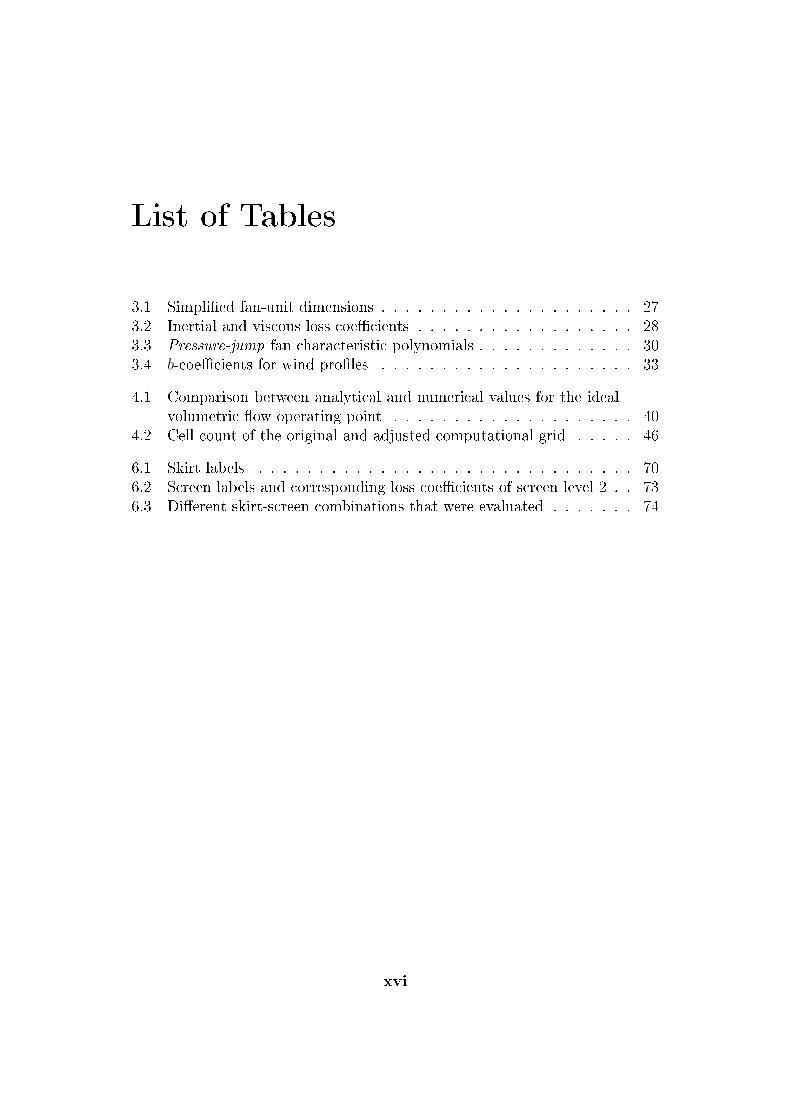
List of Tables
3.1 Simpli�ed fan-unit dimensions . . . . . . . . . . . . . . . . . . . . . 273.2 Inertial and viscous loss coe�cients . . . . . . . . . . . . . . . . . . 283.3 Pressure-jump fan characteristic polynomials . . . . . . . . . . . . . 303.4 𝑏-coe�cients for wind pro�les . . . . . . . . . . . . . . . . . . . . . 33
4.1 Comparison between analytical and numerical values for the idealvolumetric �ow operating point . . . . . . . . . . . . . . . . . . . . 40
4.2 Cell count of the original and adjusted computational grid . . . . . 46
6.1 Skirt labels . . . . . . . . . . . . . . . . . . . . . . . . . . . . . . . 706.2 Screen labels and corresponding loss coe�cients of screen level 2 . . 736.3 Di�erent skirt-screen combinations that were evaluated . . . . . . . 74
xvi

Nomenclature
Constants
𝜋 = 3.141 592 654
Variables
𝐴 Area . . . . . . . . . . . . . . . . . . . . . . . . . . . . . . . [m2 ]
𝑎 Variable . . . . . . . . . . . . . . . . . . . . . . . . . . . . . [ ]
𝑏 Variable . . . . . . . . . . . . . . . . . . . . . . . . . . . . . [ ]
𝐶 Inertial loss coe�cient . . . . . . . . . . . . . . . . . . . . [ ]
𝑐𝑝 Speci�c heat . . . . . . . . . . . . . . . . . . . . . . . . . . [ J/kg ⋅K ]
𝑑 Diameter . . . . . . . . . . . . . . . . . . . . . . . . . . . . [m ]
𝐻 Height . . . . . . . . . . . . . . . . . . . . . . . . . . . . . . [m ]
ℎ Convection heat transfer coe�cient . . . . . . . . . . . . . [W/m2 ⋅K ]
𝑖 Variable . . . . . . . . . . . . . . . . . . . . . . . . . . . . . [ ]
𝑗 Variable . . . . . . . . . . . . . . . . . . . . . . . . . . . . . [ ]
𝐾 Loss coe�cient . . . . . . . . . . . . . . . . . . . . . . . . . [ ]
𝑘 Thermal conductivity . . . . . . . . . . . . . . . . . . . . . [W/m ⋅K ]
𝐿 Length . . . . . . . . . . . . . . . . . . . . . . . . . . . . . . [m ]
𝑚 Mass�ow . . . . . . . . . . . . . . . . . . . . . . . . . . . . [ kg/s ]
𝑁 Rotational speed . . . . . . . . . . . . . . . . . . . . . . . . [ rev/min ]
𝑁𝑦 Heat transfer parameter . . . . . . . . . . . . . . . . . . . [ 1/m ]
𝑛 Number . . . . . . . . . . . . . . . . . . . . . . . . . . . . . [ ]
𝑃 Power . . . . . . . . . . . . . . . . . . . . . . . . . . . . . . [W ]
𝑝 Pressure . . . . . . . . . . . . . . . . . . . . . . . . . . . . . [N/m2 ]
𝑄 Heat . . . . . . . . . . . . . . . . . . . . . . . . . . . . . . . [W ]
𝑞 Heat �ux . . . . . . . . . . . . . . . . . . . . . . . . . . . . [W/m2 ]
𝑅𝑦 Flow parameter . . . . . . . . . . . . . . . . . . . . . . . . [ 1/m ]
𝑆 Source term . . . . . . . . . . . . . . . . . . . . . . . . . . . [ ]
𝑇 Temperature . . . . . . . . . . . . . . . . . . . . . . . . . . [K ]
xvii

NOMENCLATURE xviii
𝑈𝐴 Overall heat transfer coe�cient . . . . . . . . . . . . . . . [W/m2 ]
𝑢 x-direction velocity . . . . . . . . . . . . . . . . . . . . . . [m/s ]
𝑉 Volume, Volume�ow . . . . . . . . . . . . . . . . . . . . . . [m3,m3/s ]
𝑣 Velocity, y-direction velocity . . . . . . . . . . . . . . . . . [m/s ]
𝑤 Work, z-direction velocity . . . . . . . . . . . . . . . . . . . [W/m2,m/s ]
𝑥 Coordinate . . . . . . . . . . . . . . . . . . . . . . . . . . . [m ]
Greek symbols
1/𝛼 Viscous loss coe�cient . . . . . . . . . . . . . . . . . . . . [ ]
𝛽 Fan blade angle (measured at fan tip), Thermal expansion coe�-cient . . . . . . . . . . . . . . . . . . . . . . . . . . . . . . . . [ ∘, 1/K ]
Γ Di�usion coe�ecient . . . . . . . . . . . . . . . . . . . . . [ ]
𝜀 E�ectiveness . . . . . . . . . . . . . . . . . . . . . . . . . . [ ]
𝜁 Fan blade angle (measured at fan hub) . . . . . . . . . . . [ ∘ ]
𝜃 Angle . . . . . . . . . . . . . . . . . . . . . . . . . . . . . . [ ∘ ]
𝜇 Viscosity . . . . . . . . . . . . . . . . . . . . . . . . . . . . . [ kg/m ⋅ s ]𝜌 Density . . . . . . . . . . . . . . . . . . . . . . . . . . . . . [ kg/m3 ]
𝜎 Ratio . . . . . . . . . . . . . . . . . . . . . . . . . . . . . . . [ ]
Φ Energy dissipation term . . . . . . . . . . . . . . . . . . . [ ]
𝜙 Variable . . . . . . . . . . . . . . . . . . . . . . . . . . . . . [ ]
Dimensionless groups
Pr Prandtl number . . . . . . . . . . . . . . . . . . . . . . . . [ ]
Re Reynolds number . . . . . . . . . . . . . . . . . . . . . . . [ ]
Vectors and Tensors
u Velocity vector . . . . . . . . . . . . . . . . . . . . . . . . . [m/s ]
Subscripts
𝑎 Air
𝑏 Bundle, bellmouth, blade
𝑐 Casing, contraction
𝑐𝑟 Chord
𝑑 Dynamic
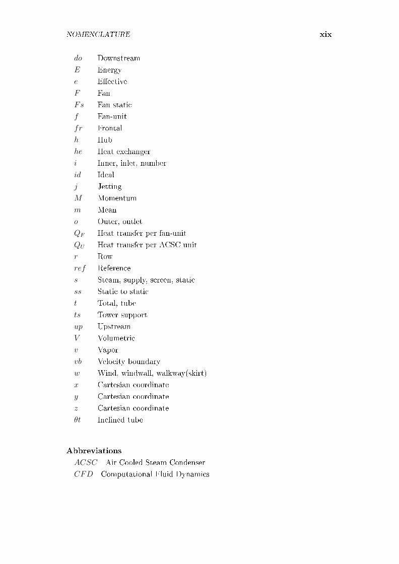
NOMENCLATURE xix
𝑑𝑜 Downstream
𝐸 Energy
𝑒 E�ective
𝐹 Fan
𝐹𝑠 Fan static
𝑓 Fan-unit
𝑓𝑟 Frontal
ℎ Hub
ℎ𝑒 Heat exchanger
𝑖 Inner, inlet, number
𝑖𝑑 Ideal
𝑗 Jetting
𝑀 Momentum
𝑚 Mean
𝑜 Outer, outlet
𝑄𝐹 Heat transfer per fan-unit
𝑄𝑈 Heat transfer per ACSC unit
𝑟 Row
𝑟𝑒𝑓 Reference
𝑠 Steam, supply, screen, static
𝑠𝑠 Static to static
𝑡 Total, tube
𝑡𝑠 Tower support
𝑢𝑝 Upstream
𝑉 Volumetric
𝑣 Vapor
𝑣𝑏 Velocity boundary
𝑤 Wind, windwall, walkway(skirt)
𝑥 Cartesian coordinate
𝑦 Cartesian coordinate
𝑧 Cartesian coordinate
𝜃𝑡 Inclined tube
Abbreviations
𝐴𝐶𝑆𝐶 Air-Cooled Steam Condenser
𝐶𝐹𝐷 Computational Fluid Dynamics

NOMENCLATURE xx
𝑈𝐷𝐹 User De�ned Function

Chapter 1
Introduction
1.1 Background
Thermodynamic cycles are used to harness energy from a heat source be itthe sun, coal, nuclear or natural gas. In a thermodynamic cycle, work isdone by continuously adding and extracting heat to and from a working �uid.The Rankine cycle, depicted in �gure 1.1, has been widely adapted for use inthe power generating industry where steam is utilized as an energy conveyingmedium.
Figure 1.1: Rankine energy cycle (Adapted from Cengel and Boles (2006))
In a typical Rankine cycle, �uid is pumped to a boiler where heat is trans-ferred to this �uid from a natural source e.g. coal. The �uid heats up andultimately leaves the boiler as superheated vapor. After this, work is obtained
1

CHAPTER 1. INTRODUCTION 2
by allowing the vapor to expand in a turbine (or series of turbines). To com-plete the cycle, vapor exhausted from the turbine, is condensed in a condenser,rejecting unused heat.
Cengel and Boles (2006) mentions that steam is the most common working�uid used in vapor power cycles due to its multitude of desirable characteris-tics. Amongst these characteristics are its relatively low cost, availability andhigh enthalpy of vaporization. According to Kröger (2004) and Al-Waked andBehnia (2003) steam cycle power stations reject about 45 % of the initial heatinput through a condenser, while approximately 15 % is rejected through thestack. It is therefore clear that dedicated attention be given to the design ofe�ective cooling systems, since it plays an important part in the generatingcapacity of a power station.
Two main types of cooling exist, categorized as wet- and dry-cooling. Wet-cooling is the means of cooling with a �uid, which ordinarily is water. Ac-cording to Bartz and Maulbetsch (1981), 75 % of coal-�red power plants builtbefore 1970 used once-through cooling, relying on large water bodies such asoceans, dams or rivers, as energy sinks. An alternative to once-through cool-ing is found by means of wet-cooling towers depicted in �gure 1.2 (a). Heatedcooling water is sprayed onto a �ll in the cooling tower which assists the pro-cess of evaporation. Evaporation is attained by means of a constant naturaldraft through the cooling tower. The water is cooled in this way and rains intoa water basin from where it is returned to the condenser. Although this typeof cooling provides a relatively high thermal e�ciency (Tawney et al., 2005), aproblem emerges since fewer inland locations are able to support the massivewater demand and strict environmental regulations complicates this coolingapproach (Akhtar, 2000),(Swanekamp, 2002). Water consumed by these powerstations for make-up water, cooling tower blowdown and ash scrubbing, is inthe order of 2.5 l/kWh, which is a considerable amount compared to 0.2 l/kWhconsumed by dry-cooled systems (Knirsch, July 1991). Due to the mentionedconcerns regarding water, an increasing interest towards dry-cooling is noticed(EPRI, 2005).
Dry-cooling is an alternative to wet-cooling and �nds increasing interest dueto its water e�ciency and practicality in arid areas. Cooling is provided bymeans of ambient air, removing heat from a thermal cycle through convection.Although various types of dry-cooling exist in steam cycle power stations, onlyforced draft air-cooled steam condensers (ACSC's) will be discussed, since thepresent research involves this cooling method.
A steam power generation cycle, with the utilization of ACSC's for cooling,is shown in �gure 1.3. A typical ACSC, consists of a number of �nned tubebundles arranged in an A-frame formation to reduce the total plant surface
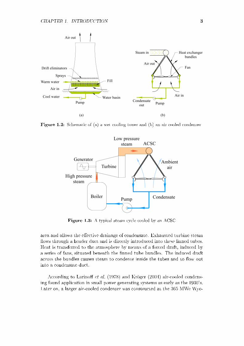
CHAPTER 1. INTRODUCTION 3
Figure 1.2: Schematic of (a) a wet-cooling tower and (b) an air-cooled condenser
Figure 1.3: A typical steam cycle cooled by an ACSC
area and allows the e�ective drainage of condensate. Exhausted turbine steam�ows through a header duct and is directly introduced into these �nned tubes.Heat is transferred to the atmosphere by means of a forced draft, induced bya series of fans, situated beneath the �nned tube bundles. The induced draftacross the bundles causes steam to condense inside the tubes and to �ow outinto a condensate duct.
According to Larino� et al. (1978) and Kröger (2004) air-cooled condens-ing found application in small power generating systems as early as the 1930's.Later on, a larger air-cooled condenser was constructed at the 365 MWe Wyo-

CHAPTER 1. INTRODUCTION 4
dak power station near Gilette in the USA, which consisted of 11 x 6 fans plusan extra prototype row of 6 fans. This plant came into operation in 1978 andheld some challenges due to it's high altitude above sea level (1240 m) andextreme climatic temperatures of −40 ∘C to 43 ∘C. Knirsch (July 1991) andKröger (2004) both report that it was the largest ACSC built at that timeand held this status until the 6 x 665 MWe Matimba power station came intooperation in 1991.
Due to the coal rich environment, South Africa's main electricy supplier(ESKOM), made the decision to construct the Matimba power station in Lep-helale, South Africa. However, a local de�ciency of water led to the construc-tion of the current largest forced draft air-cooled power station in the world.
Matimba's ACSC consists of elliptic �nned tube bundles arranged in anA-formation on top of 288 axial �ow fans with a diameter of approximately9 m and is situated at an elevation of 45 m above ground level. The entireACSC covers a plan area of 32 300 m2 and is placed against the turbine hallas can be seen in �gure 1.4. This placement favors condenser performanceduring dominant Easterly winds, since air is obstructed by the turbine halland forced upwards into the ACSC. However, Goldschagg (1993) reports thatadverse ambient conditions such as strong winds, Westerly winds and extremetemperatures greatly a�ect the performance of the Matimba ACSC due to hotplume recirculation and poor fan performance as a consequence of distortedair in�ow on the periphery of the ACSC.
Figure 1.4: 3990 MWe Matimba power station
Due to a mentioned global tendency toward dry-cooling, further investiga-

CHAPTER 1. INTRODUCTION 5
tion is required in order to optimize ACSC performance for the widest rangeof atmospheric conditions.
1.2 Literature survey
The literature survey of the present study follows in a chronological order andshows the development of forced draft air-cooled heat exchanger technology.
An article was released by Monroe (1979) on improving the overall ef-fectiveness of air-cooled heat exchangers. It was noticed that among otherproblems in heat exchanger design speci�cations, a reduction in system per-formance also occurred due to hot plume recirculation (�gure 1.5). This wasespecially noticed in forced draft air-coolers where low exit velocities are evi-dent. It was also found that mechanical energy losses, due to �ow separationat the fan inlets, reduce fan performance. It was recommended that the airvelocity, approaching the heat exchanger, should not exceed half of the veloc-ity through the fan throat. The article proposed that recirculation would bereduced by the implementation of ba�es (windwalls) at the �ow exit as wellas to increase the exit �ow velocity.
Figure 1.5: Schematic of plume recirculation and �ow separation
Kröger (1989) analytically, numerically and experimentally investigatedthe reduction of performance in a mechanical draft heat exchanger due to re-circulation. A two-dimensional model was considered for which an equation

CHAPTER 1. INTRODUCTION 6
is presented to calculate the approximate e�ectiveness of a generic heat ex-changer. This equation was derived as a function of the �ow, thermal andgeometric characteristics of the heat exchanger excluding the in�uence of mix-ing and heat transfer in the air. Kröger (1989) concluded that experimentallypredicted values followed a similar trend to the values obtained analytically,but were generally found to be higher. Mention was made that the accuracyof the experimental results could possibly have been a�ected by the size con-straint of the test facility, used to model a scaled version of the heat exchanger.Numerical predictions included heat transfer and �ow mixing, and these valueswere generally lower than values abtained by the other two methods.
Regarding mechanical energy losses through heat exchangers, Van Aarde(1990) conducted experiments on the air �ow through a forced draft A-frameheat exchanger in which certain �ow correlations and pressure loss coe�cientswere derived. It was concluded that �ow through the heat exchanger is in�u-enced by the semi-apex angle of the bundle arrangement, the loss coe�cientthrough the bundle, the steam pipe diameter and the distance between sepa-rate A-frames. Notably atmospheric winds also had a signi�cant e�ect on theperformance of the heat exchanger.
Similar work to that of Kröger (1989) was done by Conradie (1991) whoconducted a two-dimensional analytical and full scale experimental investiga-tion (at Matimba power station, South Africa) into hot plume recirculation.Once again equations were derived to approximate performance evaluations ofair-cooled heat exchangers subject to plume recirculation. The study revealsthat the proper orientation and layout of a heat exchanger with respect tonearby structures, local topography and prevailing winds, will lead to a reduc-tion in plume recirculation.
As mentioned in section 1.1, Goldschagg (1993) con�rms plume recircu-lation occurring at the condenser of Matimba power station, South Africa, dur-ing adverse winds. The lack of su�cient cooling ultimately led to a detrimentalincrease in turbine back-pressure and sometimes turbine trips. Certain struc-tural and other modi�cations were undertaken, which ultimately improved thecondenser performance under these conditions.
Du Toit et al. (1993) studied the in�uence of the air �ow pattern inthe vicinity of a mechanical-draft heat exchanger subject to cross-wind. Atwo-dimensional model was solved by means of computational �uid dynamics(CFD), in which the e�ect of di�erent platform heights and wind speeds onoverall heat exchanger performance was investigated. It was concluded thatrecirculation has a signi�cant e�ect on the performance of the heat exchangerand that heat transfer should be based on the local �ow conditions as well asthe in�uence of the �ow �eld on the fans. It was recommended that a further
CHAPTER 1. INTRODUCTION 7
study should be done in three dimensions in order to obtain a better under-standing of the problem.
The literature to this point o�ered many solutions to plume recirculationoccurring at air-cooled heat exchangers, but no focus was placed on fan per-formance. A focus on the design and performance of axial �ow fans for the usein forced draft air-cooled heat exchangers were yet unknown and thus someinvestigation into this �eld commenced.
Thiart and Von Backström (1993) developed an actuator-disk fanmodel which uses blade element theory to numerically predict the �ow �eld inthe vicinity of the fan blades without explicitly modeling the blade geometry.The model showed good correlation to experimental results for normal axisy-metric �ow into the fan, but deviated for cases of cross-�ow beneath the faninlet. It was also mentioned that this method was computationally expensiveto use and further investigation was required to make this method viable forengineering purposes.
Bruneau (1994) designed a robust axial �ow fan for cooling tower appli-cations, solely to tolerate distorted inlet �ows. The fan, based on the NASALS aerofoil pro�le, was consequently named the B-fan. Fan tests were con-ducted according to British standard BS 848 (Type A) in order to validatethe fan performance in comparison with other industrial fan types for similarapplications. Results obtained for the B-fan indicated a higher design pointstatic e�ciency and static pressure rise compared to the other fans. However,Bruneau (1994) mentions that fan testing occurred under ideal circumstances.Further testing was needed to determine the fan performance under distortedinlet conditions.
Salta and Kröger (1995) conducted two-dimensional experiments to re-search the reduction in volume �ow rate through a single street of fans in anair-cooled heat exchanger by varying the distance between ground level andthe fan platform. The results led to the derivation of empirical correlations forheat exchanger volume �ow rate as a function of platform height. An expo-nential increase in volume �ow rate was noticed as the fan platform was raised.The addition of a skirt next to the periphery fan also signi�cantly improvedthe volume �ow rate through the edge fan, especially at low platform heights.
Duvenhage et al. (1995) conducted a numerical and experimental in-vestigation to determine the e�ect of distorted in�ow on fan performance ina forced draft air-cooled heat exchanger. Similar to Salta and Kröger (1995),Duvenhage et al. (1995) found that changes in fan platform height caused sim-ilar changes in volume �ow through the fans. Three di�erent fan inlet shroudswere also investigated i.e. Cylindrical, Conical and Bell type inlet. Since me-

CHAPTER 1. INTRODUCTION 8
chanical losses through the Bell type inlet was in the order of zero it proved tobe superior in comparison with the other inlet types. It was concluded that theinlet shroud be carefully chosen when a forced-draft ACSC is being designed.
Work done by Meyer and Kröger (2001a) involved experiments on dif-ferent types of �nned-tube heat exchangers determining to what extent the airin�ow angle across the heat exchanger in�uenced the pressure loss coe�cient.Separation was noticed at the leading edge between two �ns which increased asthe air inlet angle increased. A correlation was derived for the heat exchangerpressure loss coe�cient, concluding that it is mainly in�uenced by the tubecross-sectional area.
Stinnes and Von Backström (2002) experimentally tested air-cooledheat exchanger fans in a test tunnel, according to British standard BS 848(Type A). These tests were done to determine the e�ect of o�-axis in�ow onfan performance up to an angle of 45 ∘. It was found that these di�erent in�owangles had a negligible e�ect on fan power consumption as well as total-to-totalstatic pressure rise. However, the e�ect of distorted air in�ow, inlet bellmouthsand skirts were beyond the scope of the research.
Additional work was done by Meyer and Kröger (2003) to determineto what extent fan performance characteristics in�uenced the plenum chamberaerodynamic behavior. Numerical simulation of the mentioned B-fan was doneusing the �actuator disk� model as presented by Meyer and Kröger (2001b).The numerical study revealed that aerodynamic behavior is highly e�ected bythe type of fan, the mounted angle of the fan blades as well as the volume �owthrough the fan and thus the maximum kinetic energy recovery in the plenumdoes not necessarily coincide with the maximum fan static e�ciency.
Meyer (2005) numerically investigated the e�ect of inlet �ow distortionson fan performance in a multi-row air-cooled heat exchanger. In some instancescomparison was found with the work of Duvenhage et al. (1995) and Salta andKröger (1995). It was also con�rmed that the �rst row of fans is a�ected themost, but that a skirt on the periphery of the fan platform improves �ow intothe axial fan by moving the point of �ow separation away from the fan inletshroud.
Bredell (2005, 2006) numerically investigated the performance of twodi�erent axial �ow fans for the application in ACSC's by essentially modelinga two-dimensional street of fan units, situated in a typical section of an ACSC,using the �actuator disk� model. Once again it was shown that cross-�ow be-neath the fan platform resulted in separation and distortion of �ow at faninlets, which reduced the volumetric �ow rate through the fans nearest to theACSC upstream periphery. This �ow rate was also dependent on the type of

CHAPTER 1. INTRODUCTION 9
fan. Mention is made that the addition of a solid (non-porous) skirt along theside and a porous screen beneath the ACSC signi�cantly improves the air �owthrough the entire condenser and subsequently also the thermal e�ectiveness.
Gu et al. (2005) and Gu et al. (2006) experimentally analyzed thewind e�ects on a scale model of a large ACSC of a speci�c power plant inChina using a wind tunnel. As with Matimba, the ACSC is situated next tothe turbine hall and boiler houses. It was once again con�rmed that plumerecirculation could be minimized through an increase in windwall as well asACSC platform height.
Hotchkiss et al. (2006) continued the research of Stinnes and Von Back-ström (2002) by numerically simulating the oblique �ow of air into the fan,using the �actuator disk� fan model of Meyer and Kröger (2001b). The numeri-cal solutions con�rmed similar trends to the experimental results of Stinnes andVon Backström (2002), but slightly under- and over-predicted the fan powerconsumption and fan static e�ciency respectively. The numerical model thusproved relatively accurate up to an angle of 45 ∘.
Van Rooyen (2007, 2008) investigated the performance of a generalACSC, consisting of 30 fan units, under windy conditions from di�erent direc-tions. Once again the �actuator disk� model was employed through CFD inorder to model the fans in the condenser. Due to a limited amount of compu-tational power, three-dimensional modeling of the entire ACSC was done bysimulating some of the individual fans, whereafter a number of interpolationschemes were used to obtain values for the fans not modeled. Separation of�ow at the ACSC periphery and hot plume recirculation was noticed and trendwise showed similarities with the work of Bredell (2005). Van Rooyen (2007)also con�rmed the following:
� A marginal reduction in ACSC performance could be seen due to hotplume recirculation.
� The ACSC performance was adversely a�ected by the shortage of ambi-ent air through some fan units on the ACSC periphery due to separation.
� Modi�cations such as skirts on the ACSC periphery and porous screensbelow the ACSC improved the overall performance under windy condi-tions.
Liu et al. (2009) numerically investigated the e�ect of wind on recir-culation occurring at a power plant in China. The entire ACSC as well assurrounding buildings were modeled using CFD through which it was shownthat adverse plume recirculation occurred during strong winds, especially if
CHAPTER 1. INTRODUCTION 10
the ACSC is situated downstream of the boiler houses. Overall ACSC per-formance was also enhanced by increasing periphery fan speed to force moreambient air through these fan units during windy conditions.
Similar research to Liu et al. (2009) was done by Gao et al. (2009) whonumerically simulated the e�ect of wind on the performance of a similar ACSC.However Gao et al. (2009) focused on fan performance as well as plume recir-culation. The obtained results showed that ACSC performance was the worstfor the case where wind blew onto the ACSC from across the power stationbuildings where recirculation was the main contributor to the reduced ACSCperformance.
The ACSC of Van Rooyen (2007), consisting of 30 fan units, was alsonumerically investigated by Joubert (2010) to determine and improve theoverall performance of the ACSC by mainly improving the fan performance.Unlike Van Rooyen (2007), Joubert (2010) held a greater amount of compu-tational power and solved the �ow through all the fans in the ACSC simul-taneously using the �pressure-jump� method for fan modeling. This methodwas preferred to avoid the computationally expensive �actuator disk� modeland was justi�ed by correlation to the work of Van Rooyen (2007) in mostcases, with some exception in cases with high wind velocities. Many additionsand modi�cations were made to the general ACSC to investigate the individ-ual e�ects on fan performance such as ACSC height variation, bellmouth inletalternatives, di�erent fan types and the addition of a variety of skirts alongthe periphery of the ACSC and porous screens below the ACSC. Once again itwas found that the addition of skirt along the periphery of the ACSC and theinstallation of a porous screen below the ACSC posed the most cost e�ectiveand practical solution. These modi�cations resulted in an increase of 11.3 %in ACSC performance compared to the poorest performance of the unmodi�edACSC.
Owen (2010) developed a two-step numerical modeling approach to inves-tigate the performance of an ACSC also evading the computationally expensive�actuator disk� fan model by using the �pressure-jump� method. The ACSCof El Dorado power station in Nevada, USA, consisting of 30 fan units, wasnumerically modeled to simulate wind e�ects on its overall performance. Nu-merical results were found to be in good agreement with measurements takenon site. Owen (2010) mentions that reduced fan performance evidently has afar more signi�cant in�uence on ACSC performance than plume recirculation.The advantage of modi�cations such as a periphery skirt and porous screensbelow the ACSC was con�rmed. It was found that increasing the fan powerof the periphery fans under windy conditions has a limited bene�t, but mightbe valuable if it is considered in the design phase of an ACSC.

CHAPTER 1. INTRODUCTION 11
A thorough understanding of the �ow �eld and associated phenomenaabout a mechanical-draft heat exchanger is imperative for optimal design ofsuch a system (Du Toit et al., 1993). Literature ((Kröger, 1989), (Du Toitet al., 1993), (Hotchkiss et al., 2006), (Bredell, 2005), (Van Rooyen, 2007),(Liu et al., 2009), (Owen, 2010) and (Joubert, 2010)) has shown that CFDsimulation can e�ectively be implemented to obtain better knowledge of the�ow �eld around such heat exchangers and ultimately provide valuable infor-mation to estimate heat exchanger performance.
1.3 Research objective
E�ciency is a main concern in any thermal cycle and consequently also inpower stations. E�cient cooling in a power station promotes e�cient elec-tricity production. With the mentioned trend towards dry-cooling and theconstruction of large ACSC's such as Matimba, a need arises to investigatethe performance of these large systems, especially under windy conditions,since a signi�cant reduction in performance occurs under these circumstances.Owen (2010) mentions that experiments on such large systems can amount tosigni�cant costs. Thus a seemingly cheaper and easier alternative is the use ofCFD simulation.
Previous research done by Bredell (2005), Van Rooyen (2007), Owen (2010)and Joubert (2010) simulated the e�ect of distorted fan in�ow on overall ACSCperformance. The work of Bredell (2005) and Van Rooyen (2007) providedvaluable insight into the numerical simulation of fans and ACSC's. This cre-ated a foundation for the work of Owen (2010) and Joubert (2010) who suc-cessfully simulated the e�ect of wind on full scale ACSC's consisting of 30 fans.
The present research project attempts to further this research by investi-gating the wind e�ect on an ACSC similar (but not identical) to the ACSCof the 4800 MWe Medupi (Pretorius and Du Preez, 2009) steam cycle powerplant shown in �gure 1.6. The ACSC consists of 384 individual fan units andhas an overall surface footprint of approximately 72300 m2. The investigatedACSC will conveniently be referred to as the Large ACSC throughout the re-mainder of the present study.
It should be mentioned that, due to a limit in computational resources,some simpli�cations to the numerical condenser model were made in the presentstudy. These simpli�cations and numerical procedures will be discussed ingreater detail in chapter 3.
As a �rst attempt, the numerical modeling (done in commercial code, Flu-

CHAPTER 1. INTRODUCTION 12
Figure 1.6: Schematic of the Medupi ACSC
ent 12 ) of the Van Rooyen (2007) ACSC system will be repeated to gaincon�dence in the numerical procedure used for the present research. Resultsobtained from this simulation will then be compared to results of Van Rooyen(2007), Owen (2010) and Joubert (2010) in order to con�rm the validity ofthis numerical approach. Once the ACSC of Van Rooyen (2007) is success-fully simulated the numerical modeling of the Large ACSC will commence inorder to determine the e�ect of wind on the e�ectiveness the large ACSC.
The main objectives of the present study are set out as follow:
� Design of a simpli�ed numerical ACSC models, without platform sup-ports, steam ducts and other support structures in the ACSC. Thesemodels will be used for the investigation of ACSC e�ectiveness duringwindy conditions
� Investigate the e�ect of wind on the e�ectiveness of a free standing ACSC(without the placement of the building) using symmetry for two winddirections to show general �ow e�ects occurring in the vicinity of theACSC and recognize a performance trend.
� Investigate the e�ect of power station buildings on the e�ectiveness ofthe large ACSC using symmetry for the case of one wind direction.

CHAPTER 1. INTRODUCTION 13
� Subsequently the individual and combined e�ect of various skirt andscreen con�gurations along the periphery and beneath the freestandingACSC, as well as the ACSC with the building located, will be investi-gated.

Chapter 2
ACSC system description
2.1 Applicable system details
The two air-cooled systems investigated in this study namely, Van Rooyen(2007) and the Large ACSC, di�er in a number of ways. General dimensionsand layout of both these systems are shown hereafter, while heat-exchanger,fan speci�cations and operating conditions are given in appendix A.
2.1.1 Van Rooyen (2007) ACSC
The Van Rooyen (2007) ACSC system, depicted in �gure 2.1, forms one cool-ing unit (provides cooling for one turbine-generator unit) and consists of anarray of 5× 6 = 30 fans with a series of heat-exchanger bundles in an A-typecon�guration downstream of the fans. For convenience the position of eachfan is numbered by (i,j), where i is referred to as the street (x-direction) andj the row (y-direction) in which the fan is located, if the indicated coordinatesystem is used.
Figure 2.1: General layout and dimensions of the Van Rooyen (2007) ACSC
14

CHAPTER 2. ACSC SYSTEM DESCRIPTION 15
Figure 2.2: General layout and dimensions of the Large ACSC

CHAPTER 2. ACSC SYSTEM DESCRIPTION 16
2.1.2 Large ACSC
The general layout and dimensions of the Large ACSC is shown in �gure 2.2,where 6 cooling units can be seen. Each cooling unit consists of 8× 8 = 64fans together with the heat-exchanger bundles con�gured in a similar mannerto that described previously and serves one turbine-generator unit. Once againthe speci�c position of a fan is numbered by (i,j), where i is the street and jthe row in which the fan is located.
2.2 System components
An ACSC primarily consists of an arrangement of �fan-units�. One �fan-unit�consists of one fan together with a number of heat exchanger bundles. Anexample of a typical fan unit situated on the periphery of an ACSC is shownin �gure 2.3, depicting it's main components.
During operation, an electrically driven fan draws atmospheric air upwardover a wire screen and through a bell mouth inlet before it reaches the fan.Downstream of the fan, the �ow is obstructed by the fan bridge, support struc-tures and the heat-exchanger. The �ow exiting the heat-exchanger is thende�ected upwards into the atmosphere. Figure 2.3 also shows the placementof a windwall, which is normally �xed to the periphery of an ACSC, primarilyto reduce plume recirculation.
2.2.1 Axial fan
Axial fans used in large cooling plants are unique due to their size. These fansdisplace large volumes of air at a relatively low pressure di�erence across thefan. According to Bredell (2005), aspects such as noise generation, structuralstrength and cost of these fans are important when large cooling plants aredesigned.
A scale version of these cooling fans is normally tested in a fan test facil-ity according to one of many existing test standards such as British standard848 (British Standard 848, 1997) or AMCA (Air Moving and ConditioningAssociation, (AMCA, 1975)). It needs to be noted that these tests rendera fan characteristic for undistorted in�ow conditions. This is not necessarilythe operating condition fans are subjected to in practice, especially in ACSC'swhere air approaching certain fan inlets is distorted due to the e�ect of windor induced cross-�ow from surrounding fans (Salta and Kröger, 1995).
Two di�erent eight-bladed fans were considered in the present study, namelythe B-fan (Bruneau, 1994) for application in the Van Rooyen (2007) ACSC and
CHAPTER 2. ACSC SYSTEM DESCRIPTION 17
Figure 2.3: A typical ACC fan unit
a commercially available fan for the Large ACSC. Due to the con�dentialityof the present study, the latter fan will be referred to as the L-fan. Fan in-stallation speci�cations as well as characteristics of these fans are given inappendix A.
2.2.2 Heat-exchanger bundles
A single fan-unit consists of number of A-type con�gured heat-exchanger bun-dles downstream of the axial �ow fan. These condenser bundles consist of�nned tube rows, which are connected to a steam header duct at the top and acondensate drain duct at the bottom. Steam entering the �nned tubes throughthe header duct, condenses and �ows out into the condensate drain duct.
Flattened mild steel tubes with aluminum �ns are used in the case of theVan Rooyen (2007) condenser, whereas elliptically cross-sectioned galvanizedmild steel tubes with rectangular �ns are used in the Large ACSC. The heat-exchanger bundles consist of two rows of �nned tubes in a staggered arrange-ment, as can be seen in �gure 2.3. A smaller �n pitch on the downstream(second) tube row compared to the upstream (�rst) tube row result in a nearuniform condensation rate between these successive rows. This reduces non-
CHAPTER 2. ACSC SYSTEM DESCRIPTION 18
condensible gas back-�ow from the downstream row to the upstream row,which is a problem commonly found in multi-row condensers (Kröger, 2004).
The heat-exchanger bundle speci�cations for the Van Rooyen (2007) ACSCis given in appendix A, whereas the speci�cations for the Large ACSC areomitted due to con�dentiality.
2.3 Flow and heat transfer analysis
According to Bredell (2005) an ACSC has to condense a certain amount ofsteam, in order for turbine operation to occur e�ciently. The cooling providedby a single fan-unit is a function of the air mass �ow provided by the fan aswell as the inlet air temperature to the heat-exchanger bundles. Inherently theamount of cooling provided by an entire ACSC cooling unit could therefore bequanti�ed as the summation of the cooling provided by each fan-unit.
2.3.1 Flow calculation
The air �owing through the ACSC is subject to mechanical energy losses. Eachloss can be de�ned by a loss coe�cient, 𝐾, given as
𝐾 =Δ𝑝
𝜌𝑣2/2(2.3.1)
where 𝑣 is the �ow velocity based on a certain �ow area.The draft equation for a single fan unit is speci�ed as
𝑝1 − 𝑝7 =
𝐾𝑡𝑠
(𝑚𝑎
𝐴𝑡𝑓𝑟
)2
2𝜌𝑎1+
𝐾𝑢𝑝
(𝑚𝑎
𝐴𝑒
)2
2𝜌𝑎3−Δ𝑝𝐹𝑠 +
𝐾𝑑𝑜
(𝑚𝑎
𝐴𝑒
)2
2𝜌𝑎3+
𝐾𝜃𝑡
(𝑚𝑎
𝐴𝑡𝑓𝑟
)2
2𝜌𝑎56≈ 0, 𝑁/𝑚2 (2.3.2)
The various loss coe�cients in equation (2.3.2) are discussed in greaterdetail in appendix A, whereas the fan static pressure, Δ𝑝𝐹𝑠, is given by equa-tion (B.1.1) in appendix B. Finally 𝐴𝑡𝑓𝑟 and 𝐴𝑒 is the total heat exchangerfrontal area for one fan unit and the fan annulus area respectively. 𝐴𝑡𝑓𝑟 isgiven for a certain ACSC system, whereas 𝐴𝑒 is determined as follow:
𝐴𝑒 =𝜋(𝑑2𝑐 − 𝑑2ℎ)
4,𝑚2 (2.3.3)

CHAPTER 2. ACSC SYSTEM DESCRIPTION 19
where 𝑑𝑐 and 𝑑ℎ are the fan casing and fan hub diameters respectively.
2.3.2 Heat transfer calculation
Heat transferred to the atmosphere was calculated using the 𝜀-𝑁𝑇𝑈 methodassuming the steam temperature inside the heat-exchanger bundles to remainconstant. This assumption will be discussed to more detail in section 3.4.
The energy equation is given by:
𝑄𝑎 =𝑛𝑟∑𝑖=1
𝑚𝑎𝑐𝑝𝑎(𝑖)(𝑇𝑎𝑜(𝑖) − 𝑇𝑎𝑖(𝑖)
)=
𝑛𝑟∑𝑖=1
𝜀(𝑖)𝑚𝑎𝑐𝑝𝑎(𝑖)(𝑇𝑠(𝑖) − 𝑇𝑎𝑖(𝑖)
),𝑊 (2.3.4)
where 𝑛𝑟 is the number of tube rows present in the heat-exchanger. Sincecondensation takes place inside the heat-exchanger, the e�ectiveness, 𝜀(𝑖), ofeach tube row can be calculated as follow:
𝜀(𝑖) = 1− 𝑒
( −𝑈𝐴(𝑖)𝑚𝑎𝑐𝑝𝑎(𝑖)
)(2.3.5)
In equation (2.3.5), the overall heat transfer coe�cient, 𝑈𝐴(𝑖), for a certainrow is given as
𝑈𝐴(𝑖) ≈ ℎ𝑎𝐴(𝑖) = 𝑘𝑎𝐴(𝑖)𝑁𝑦(𝑖)𝑃0.333𝑟 , 𝐽/𝐾 (2.3.6)
where ℎ𝑎𝐴(𝑖) is the e�ective heat transfer coe�cient for a certain tube row.The heat transfer parameter, 𝑁𝑦(𝑖), for a speci�c tube row is de�ned by Kröger(2004) as
𝑁𝑦(𝑖) = 𝑎𝑅𝑦𝑏(𝑖) , 1/𝑚 (2.3.7)
where 𝑎 and 𝑏 are constants unique to a tube row. The �ow parameter, 𝑅𝑦(𝑖),for each row is de�ned as
𝑅𝑦 =𝑚𝑎
𝜇𝑎𝐴(𝑖)
, 1/𝑚 (2.3.8)
Chapter 3
Numerical modeling
According to Versteeg and Malalasekera (2007), CFD (Computational FluidDynamics) could be de�ned as the analysis of systems involving (but not con-�ned to) �uid �ow and heat transfer by means of computer simulation. Thissection gives a brief overview of the governing equations of a �uid in motion.It also looks into discretization, solver settings, turbulence and buoyancy mod-eling and boundary conditions applicable to this thesis. Further aspects suchas the modeling procedures used and the means by which ACSC performancewere measured, are also discussed.
As mentioned in chapter 1 only a limited amount of computational re-sources were available. Modeling was done on a computer with two 3.16 GHzprocessors, 8 GB of RAM available and a 660 MHz graphics processing unit.Solving was maainly done on a computer cluster. Each computing node onthe cluster has eight 2.83 GHz processors, with 16 GB of RAM available. Thelargest computational domain, ≈ 12(10)6 control volumes, in the present studytook between 8 and 12 hours to complete between 900 and 1200 iterations, ifit was solved in parallel across 8 processors on the cluster. The biggest limi-tation occured on the computer where modeling took place. A rule of thumbcommonly used for meshing is to stick to a million control volumes per 1 GBof RAM. Pushing the boundaries of the model to ≈ 12(10)6 control volumes,consumed all resources on the modeling computer and often corupted the mod-eling program GAMBIT. A typical FLUENT case and data �le would also takeapproximately 30 minutes to open on this computer and take additional timeto plot results, depending on how many the user would like to view. Takingthe large amount simulations done in the present study into account, madethe long waiting periods for the computer to process data impractical. Full3D modelling of the entire power station were thus not suitable in the presentresearch.
20

CHAPTER 3. NUMERICAL MODELING 21
3.1 CFD code summary
3.1.1 Governing equations
The numerical analysis of the ACSC's under investigation was modeled withcomputer software, Fluent 12, which uses a �nite volume solution techniqueto solve the �ow �eld. Each volume is subject to the governing equations of�uid in motion. The steady state, three-dimensional governing equations of a�uid in motion, as found in Versteeg and Malalasekera (2007), are given below:
Continuity:
div(𝜌u) = 0 (3.1.1)
𝑥-momentum:
div(𝜌𝑢u) = −∂𝑝
∂𝑥+ div(𝜇 grad 𝑢) + 𝑆𝑀𝑥 (3.1.2)
𝑦-momentum:
div(𝜌𝑣u) = −∂𝑝
∂𝑦+ div(𝜇 grad 𝑣) + 𝑆𝑀𝑦 (3.1.3)
𝑧-momentum:
div(𝜌𝑤u) = −∂𝑝
∂𝑧+ div(𝜇 grad 𝑤) + 𝑆𝑀𝑧 (3.1.4)
Energy:
div(𝜌𝑖u) = −𝑝 div u+ div(𝑘 grad 𝑇 ) + Φ + 𝑆𝑒 (3.1.5)
The velocity vector u is de�ned as
u = 𝑢+ 𝑣 + 𝑤 (3.1.6)
where 𝑢, 𝑣 and 𝑤 are the velocities in the 𝑥, 𝑦 and 𝑧 directions respectivelywhen a cartesian coordinate system is used.
The momentum source terms, 𝑆𝑀𝑥, 𝑆𝑀𝑦 and 𝑆𝑀𝑧, account for all exter-nal momentum sources such as buoyancy and gravitational forces in the �uid.These source terms also account for other obstructions in the �ow path typi-cally modeled by porous media (Fluent Inc., 2006).

CHAPTER 3. NUMERICAL MODELING 22
According to Versteeg and Malalasekera (2007) all e�ects due to viscousstresses in the energy equation can be taken into account by the dissipationfunction, Φ, de�ned as
Φ = 𝜇
{2
[(∂𝑢
∂𝑥
)2
+
(∂𝑣
∂𝑦
)2
+
(∂𝑤
∂𝑧
)2]+
(∂𝑢
∂𝑦+
∂𝑣
∂𝑥
)2
+
(∂𝑢
∂𝑧+
∂𝑤
∂𝑥
)2
+
(∂𝑣
∂𝑧+
∂𝑤
∂𝑦
)2}
− 2
3𝜇(div u)2 (3.1.7)
Lastly the source term, 𝑆𝑒, in the energy equation accounts for additionalvolumetric heat sources e.g. chemical reactions or heat transfer, other thanconduction or convection between neighboring cells.

CHAPTER 3. NUMERICAL MODELING 23
3.1.2 Discretization and solver settings
The commonalities in the governing equations enables the de�nition of a gen-eral transport equation in terms of variables, 𝜙 and Γ. The general transportequation is expressed as:
div(𝜌𝜙u) = div(Γ grad 𝜙) + 𝑆𝜙 (3.1.8)
The governing equations can be obtained by setting 𝜙 equal to 1, 𝑢, 𝑣, 𝑤and 𝑖 respectively, and selecting the corresponding values for the di�usion co-e�cient, Γ. According to Versteeg and Malalasekera (2007), equation (3.1.8)is the starting point of any numerical calculation in the �nite volume methodand needs to be integrated (discretized) for individual control volumes in thecomputational domain.
The value, 𝜙, of an individual volume, is stored at the center of the vol-ume (Fluent Inc., 2006) and requires the solution of the discretized equation,unique to that volume. However, to solve the discretized equation, requires thesubstitution of boundary conditions, 𝜙𝑓 , obtained at the volume faces. Theseboundary conditions are calculated by means of a di�erencing or interpolationscheme between 𝜙 of neighboring volumes. Consequently, some iteration isrequired in order to obtain 𝜙.
Numerical computation in the present study was done using a �rst orderupwind di�erencing scheme. According to Fluent Inc. (2006), this scheme iscomputationally more stable compared to the second order upwind scheme.This advantage does however come at the expense of reduced accuracy andcould lead to problems such as numerical di�usion. The �rst order upwindscheme does however always render a realistic solution, making it an appro-priate choice for the present study, since a performance trend is investigated.
Gradients, ∇𝜙, were calculated using Green-Gauss node based gradientevaluation. This method provides second order accuracy in the evaluation ofgradients between the nodes on volume faces and is the preferred method whenunstructured grids are solved (Fluent Inc., 2006).
Pressure-velocity coupling was done using the SIMPLE algorithm, sinceit provides superior convergence for grids containing skew cells (Fluent Inc.,2006) and is therefore suitable for the unstructured grids implemented in thepresent study.
CHAPTER 3. NUMERICAL MODELING 24
3.1.3 Turbulence modeling
All �ow encountered in engineering can be characterized as turbulent or lami-nar depending on the level of chaos present in the �ow, which is an indicationof the random variation of local velocity and pressure in the �uid. Variousturbulence models exist for numerical analysis of which individual models arerelevant to di�erent types of �ow problems.
Arguably the Standard k-𝜀 turbulence model is the most popular and widelyused model in numerical computation. Despite its many advantages, suchas simplicity and countless validation, the Standard k-𝜀 turbulence modelshows poor performance in predicting swirling and rotating �ows (Versteegand Malalasekera, 2007). For this reason some variations of the Standard k-𝜀model was developed.
According to Fluent Inc. (2006) the Realizable k-𝜀 model provides superiorperformance in �ows where rotation, separation and recirculation is present.Joubert (2010) also investigated the e�ect of wind on the performance of theVan Rooyen (2007) ACSC using the Standard, RNG and the Realizable k-𝜀model. The study showed a negligible di�erence between the respective nu-merical results.
The Realizable k-𝜀 model is used for the present numerical calculation ofturbulence in the vicinity of an ACSC.
3.1.4 Buoyancy modeling
Heated air rejected to the atmosphere is subject to a change in density andconsequently some buoyancy modeling is required. Fluent provides a couple ofoptions to buoyancy modeling. The �rst option solves the local density of eachcontrol volume in relation to the temperature of the volume. This might bea more accurate approach, but is expensive since solution convergence takeslonger (Fluent Inc., 2006). The second option to buoyancy modeling is bymeans of the Boussinesq model discussed hereafter.
The Boussinesq model (equation (3.1.9)) treats density as a constant in allequations, except for the buoyancy term in the momentum equations.
𝜌 = 𝜌0(1− 𝛽(𝑇 − 𝑇0)) (3.1.9)
where 𝜌0 is the operating density, 𝑇 the local temperature, 𝑇0 the operatingtemperature and 𝛽 the thermal expansion coe�cient de�ned as a function ofthe ambient temperature:

CHAPTER 3. NUMERICAL MODELING 25
𝛽 = 1/𝑇 (3.1.10)
According to Fluent Inc. (2006) the use of the Boussinesq model providesquicker convergence than the temperature-density relation approach, but isonly valid if
𝛽(𝑇 − 𝑇0) ≪ 1 (3.1.11)
In the present study the largest value of the term on the right-hand sideof equation (3.1.11) is calculated to be 0.089, which consequently justi�es theuse of the Boussinesq model.
3.1.5 Boundary conditions
The computational domain is governed by the equations speci�ed earlier, butalso has to satisfy constants set by boundaries in the �ow domain. Di�erenttypes of boundary conditions exist, but can mainly be classi�ed as surfaceand volume based boundaries. The various boundaries used in this study arediscussed hereafter.
Wall boundaries are surfaces in the computational domain with zero porosityto �ow. Fluent enforces a default �zero-slip� condition at the �uid wallinterface, but also allows the user to model a �slip-wall�, by changing thedefault wall viscous stress settings.
Velocity boundaries allows the user to specify a �xed velocity of �uid (there-fore a �xed mass �ow) �owing into the computational domain (whetherconstant or based on a velocity pro�le) together with other propertiessuch as gage pressure and temperature. Where it is necessary, it can alsobe used to model the rate of �uid leaving the computational domain, byspecifying an outlet velocity.
Pressure boundaries require the speci�cation of �uid pressure and are usedwhere the pro�le of �uid crossing the boundary is unknown. Fluid isallowed to enter or leave the computational domain across this boundarydepending on the state of the �ow close to the boundary. Fluid enteringthe computational domain is subject to prede�ned properties, such astemperature and turbulence.
Fan boundaries were modeled using the pressure-jump method, derived in ap-pendix B. This method uses the velocity values in the control volumesimmediately upstream of the fan rotation plane to calculate a pressuredi�erence based on the user speci�ed fan characteristic polynomial. Thepressure increase is then added to the control volumes immediately down-stream of the fan rotation plane.

CHAPTER 3. NUMERICAL MODELING 26
Symmetry boundaries are located in numerical models, where the physicalgeometry and the �ow pattern of the numerical model is expected to havesymmetry. No user speci�cations are required for symmetry boundariesother than the correct boundary placement.
Interior boundaries are planes inside the computational domain, bearing acertain reference tag speci�ed by the user. These boundaries are nu-merically �transparent� and do not a�ect the �ow in any way, but couldhowever be switched to another boundary condition by the user, withoutaltering the grid volumes.
Radiator boundaries are referenced planes, similar to interior boundaries,yet these boundaries allow the user to specify a pressure di�erence andheat transfer coe�cient as functions of the normal velocity to the iden-ti�ed radiator plane.
Porous media is a boundary condition applied to a zone of identi�ed volumesin the computational domain and allows the user to alter the �ow in thiszone, by specifying energy and momentum source terms. It could beused to simulate the �ow through packed beds, �ow distributers or anyother volumetric obstacle.
3.2 Modeling of a single fan unit
As mentioned in section 2.2, an entire ACSC consists of a number of individualfan-units. The summation of individual fan-unit performances would conse-quently give the performance of the entire ACSC. It is therefore necessary tocreate a numerical fan-unit model that would accurately solve the �ow andheat transfer through a fan unit, at a reasonable computational expense.
The numerical modeling of a conventional A-frame fan unit as depictedin �gure 3.1 (a), poses some computational challenges since details such asthe inlet screen, fan bridge and other obstructions to �ow, require a �ne com-putational grid. In addition to this, the explicit modeling of the fan andheat-exchanger bundles also holds some computational complexities. Sincethe main aim of this thesis is to investigate a performance trend of an ACSCand not the �ow through the plenum chamber, such detail could be modeledwith less e�ort by implementing a simpli�ed fan-unit model similar to themodel proposed by Bredell (2005) and shown in �gure 3.1 (b).
Dimensions to the simpli�ed fan-unit model (�gure 3.1 (b)) are given intable 3.1. This simpli�ed fan-unit consists of a heat-exchanger and fan model,placed in the 𝑥𝑦-plane. Both these models will be discussed hereafter.

CHAPTER 3. NUMERICAL MODELING 27
Figure 3.1: Representation of a conventional A-frame fan-unit and its correspond-ing numerical model
Table 3.1: Simpli�ed fan-unit dimensions
System 𝑯𝒘,𝒎 𝑳𝒙,𝒎 𝑳𝒚,𝒎 𝑳𝒛,𝒎
Large ACSC 14.4 13.5 13.625 0.2
Van Rooyen (2007) 10 11.8 10.56 0.2
3.2.1 Heat-exchanger model
As can be seen in �gure 3.1 (b), detail such as supports, wire screens, fanbridges, �nned tube bundles and additional support structures are absent inthe numerical fan-unit model. Furthermore, the rectangular plenum chamberis di�erent to the A-con�guration of the fan-unit in practice, resulting in adi�erent �ow path through the fan-unit.
The one-dimensional draft equation (equation (2.3.2)) presented by Kröger(2004), does however provide a method to calculate the e�ective system re-sistance, Δ𝑝𝑒, of a single fan-unit, if the Δ𝑝𝐹𝑠 component is omitted. Thisequation accounts for the mechanical �ow losses due to the obstructions men-tioned previously as well as the �ow e�ects, such as contraction, expansionand jetting.
Since all �ow through a conventional fan-unit is eventually de�ected up-ward into the atmosphere, a rectangular plenum fan-unit model could be usedwith a downstream porous zone, where the porous zone accounts for the e�ec-tive �ow resistance through the fan unit. Moreover, a comparison was done byOwen (2010) between an A-frame and a simpli�ed fan-unit model and showed
CHAPTER 3. NUMERICAL MODELING 28
that there exists a minimal di�erence in volumetric e�ectiveness between therespective models.
The calculation of a Van Rooyen (2007) fan-unit e�ective system resistanceis shown in appendix A. A similar calculation for a Large ACSC fan-unit isomitted due to con�dentiality.
The porous zone in Fluent accounts for the �ow resistance by means ofmomentum source terms, 𝑆𝑖, added to the momentum equations and is givenas:
𝑆𝑖 = −(𝜇
𝛼𝑖
𝑢𝑖 + 𝐶𝑖1
2𝜌∣u∣𝑢𝑖
), 𝑁/𝑚3 (3.2.1)
where the footnote, 𝑖, represents the individual cartesian directions, 𝑥, 𝑦 or𝑧. 𝐶𝑖 and 1/𝛼𝑖 are the inertial and viscous loss coe�cients, respectively andshould be speci�ed by the user. The primary �ow direction through the nu-merical heat-exchanger is upward (𝑧-direction). Consequently the resistanceto �ow must be in the opposite direction.
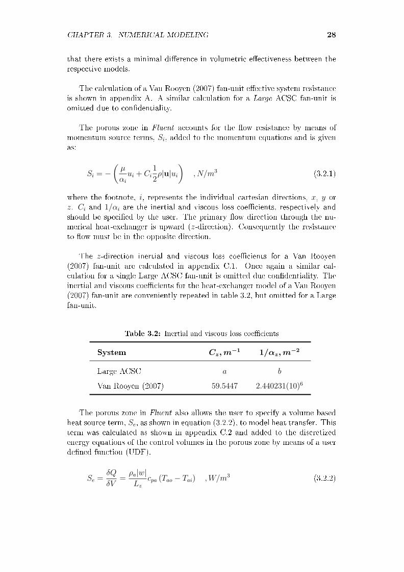
The 𝑧-direction inertial and viscous loss coe�cients for a Van Rooyen(2007) fan-unit are calculated in appendix C.1. Once again a similar cal-culation for a single Large ACSC fan-unit is omitted due con�dentiality. Theinertial and viscous coe�cients for the heat-exchanger model of a Van Rooyen(2007) fan-unit are conveniently repeated in table 3.2, but omitted for a Largefan-unit.
Table 3.2: Inertial and viscous loss coe�cients
System 𝑪𝒛,𝒎−1 1/𝜶𝒛,𝒎
−2
Large ACSC 𝑎 𝑏
Van Rooyen (2007) 59.5447 2.440231(10)6
The porous zone in Fluent also allows the user to specify a volume basedheat source term, 𝑆𝑒, as shown in equation (3.2.2), to model heat transfer. Thisterm was calculated as shown in appendix C.2 and added to the discretizedenergy equations of the control volumes in the porous zone by means of a userde�ned function (UDF).
𝑆𝑒 =𝛿𝑄
𝛿𝑉=
𝜌𝑎∣𝑤∣𝐿𝑧
𝑐𝑝𝑎 (𝑇𝑎𝑜 − 𝑇𝑎𝑖) ,𝑊/𝑚3 (3.2.2)
CHAPTER 3. NUMERICAL MODELING 29
3.2.2 Fan model
The numerical modeling of fans could be done in various ways of which twomethods, namely actuator-disk and pressure-jump methods will be discussedhereafter.
The actuator-disk numerical fan model developed by Thiart and Von Back-ström (1993) calculates momentum source terms based on blade element the-ory, applicable to �ow through the fan. These source terms are then addedto the momentum equations relevant to the control volumes in the fan model.This model has successfully been implemented in previous studies by researcherssuch as Duvenhage et al. (1995), Bredell (2005), Van Rooyen (2007) andVan der Spuy et al. (2009).
The pressure-jump fan model is the default model available in Fluent andcan simulate �ow relatively accurately with a reduced number of control vol-umes in the vicinity of the fan allowing the user to solve an array of fanssimultaneously (Van der Spuy et al., 2009). This model gives a static to staticpressure rise to the control volumes immediately downstream of an in�nitelythin fan plane, based on a user speci�ed fan characteristic polynomial (FluentInc., 2006).
As mentioned in section 1.2, Van Rooyen (2007) investigated the e�ect ofwind on an ACSC using the actuator-disk model. The same ACSC was alsoinvestigated by Owen (2010) and Joubert (2010) who both veri�ed the perfor-mance trends of Van Rooyen (2007), but implemented the pressure-jump fanmodel. Van der Spuy et al. (2009) investigated the di�erence in fan perfor-mance obtained by means of the actuator-disk and pressure-jump model fortypical fan operation in a large ACSC. This study also revealed a marginaldi�erence in fan performance between the two models, but it did not show acomparison for low air �ow rates through the fan.
The above-mentioned literature suggests that the pressure-jump model isacceptable for normal in�ow and renders results that are comparable to resultsobtained by the actuator-disk model for distorted in�ows. However literatureis vague regarding the accuracy of both these models for highly separated (ra-dial) �ow at the fan inlet and extremely low volume �ows.
Due to the uncertainty of the mentioned fan models and the greater amountof computational power required to solve a large number of fans using theactuator-disk model, a decision was made to implement the pressure-jumpmodel for the present study. This decision is justi�ed as follow:
� The number of fans a�ected by separated �ow are limited. Using the

CHAPTER 3. NUMERICAL MODELING 30
pressure-jump model would therefore lead to a relatively accurate esti-mation of an overall ACSC performance trend.
� The limit in computational resource favors the use of the pressure-jumpmodel, since it requires fewer control volumes in the vicinity of the fancompared to the actuator-disk model.
The pressure-jump fan polynomials were derived from the original total tostatic characteristic pressure curves, provided by the fan supplier, as shown inappendix B. The polynomial for the Van Rooyen (2007) ACSC is repeated intable 3.3 for convenience, but omitted for the case of the Large ACSC due tocon�dentiality.
Table 3.3: Pressure-jump fan characteristic polynomials
System Δ𝒑𝑭𝒔𝒔, 𝑵/𝒎2
Large ACSC 𝑐1𝑣2 + 𝑐2𝑣 + 𝑐3
Van Rooyen (2007) −2.63055𝑣2 + 27.2461𝑣 + 323.2303
3.2.3 Single fan-unit grid
The grid used to calculate the �ow through a single fan unit is depicted in�gure 3.2. The grid on the fan face is shown in �gure 3.2 (c). An unstructuredtetrahedral grid was chosen for the modeling procedure discussed in section 3.3.This grid type provides good accuracy and has the ability to �grow� or �shrink�in all three cartesian directions, depending on where greater accuracy is re-quired in the computational domain.
Figure 3.2: Computational grid for a single fan-unit

CHAPTER 3. NUMERICAL MODELING 31
The heat-exchanger model, consists of wedge shaped control volumes. Thisis a requirement for the UDF, calculating the heat transfered by the heat-exchanger model. The UDF extracts the velocities from Fluent on the up-stream face of the heat-exchanger model and calculates the corresponding heatsource terms. These terms are consequently added to the control volumes inthe heat-exchanger model.
Some control volumes would not have a surface situated on the upstreamface of the heat-exchanger model if tetrahedral cells were used for this purpose.This would lead to some cells in the heat-exchanger model not receiving a heatsource term, which is an inaccurate approximation to the heat transferred.
Other grid and boundary speci�cations, applicable to a single fan-unit arelisted hereafter:
� A boundary layer grid was placed on the fan side of the bellmouth inletas well as around the hub face (�gure 3.2 (c)) to simulate any e�ects ofa boundary layer if it should exist.
� The walls of the plenum chamber were modeled as slip-walls (zero frictionat the �uid-wall interface), since this is not part of the fan-unit in practiceand no mechanical energy losses will occur due to these walls.
� A zero slip condition was applied to the bellmouth faces, since no me-chanical energy losses due to this obstruction are taken into account byequation (2.3.2).
� Finally the hub was modeled as a �at face with a zero slip wall bound-ary condition for the case of the Large ACSC fan-unit, since the e�ect ofthe true hub were regarded to be negligible in the overall fan-unit per-formance. This is also justi�ed, since some uncertainty exists regardingthe fan model and therefore the detailed modeling of the hub, could beexcessive. A di�erent hub is �tted in the B-fan used for the Van Rooyen(2007) ACSC, and was modeled in the same manner.
The heat transfer and �ow of a single fan-unit was investigated analyticallyand veri�ed through numerical investigation. This �ow through the fan-unitis referred to as the ideal volume �ow rate, 𝑉𝐹𝑖𝑑, and will be discussed insection 4.1. The computational domain for thermo-�ow investigation of asingle fan-unit is shown in �gure 3.3, depicting all dimensions and domainboundaries. The height of the fan-unit above ground level, 𝐻𝑖, is unique toeach system evaluated in the present study and is given in appendix A.

CHAPTER 3. NUMERICAL MODELING 32
Figure 3.3: Computational domain for validation of a single fan-unit
3.3 Modeling procedures
Modeling of the Large ACSC poses some di�culty, since �ow in the vicinity ofthe ACSC is complicated (vortex shedding and distorted �ow), consequentlyrequiring a detail computational grid. For this reason various modeling proce-dures were investigated in an attempt to reduce the amount of computationalpower required to solve the �ow around and through the ACSC's applicable tothe present study. Symmetry was used to model the ACSC in order to save oncomputational requirements together with the Iterative modeling procedurediscussed hereafter.
3.3.1 Modeling of wind
Wind blowing across the ACSC was modeled by means of a �ow distribution atthe velocity inlet to the computational domain. This distribution is speci�edby means of the velocity pro�le given by:
𝑣𝑧 = 𝑣𝑟𝑒𝑓
(𝑧
𝑧𝑟𝑒𝑓
)𝑏
,𝑚/𝑠 (3.3.1)
where 𝑣𝑧 is the horizontal velocity magnitude at height, 𝑧 and 𝑣𝑟𝑒𝑓 is the ref-erence velocity at platform height, 𝑧𝑟𝑒𝑓 = 𝐻𝑖.
The coe�cient, 𝑏, is given in table 3.4 for the individual systems underinvestigation in the present study. It should be noted that 1/7 was usedfor investigation of the Van Rooyen (2007) ACSC. A 𝑏-coe�cient of 1/5, asrecommended by VDI (1978), was used in the present study for the largeACSC.

CHAPTER 3. NUMERICAL MODELING 33
Table 3.4: 𝑏-coe�cients for wind pro�les
System 𝒃
Large ACSC 1/5
Van Rooyen (2007) 1/7
3.3.2 Modeling procedure for the Van Rooyen (2007)ACSC
The computational domain used to model the e�ect of an 𝑥-direction wind onthe performance of the Van Rooyen (2007) ACSC is shown in �gure 3.4. This�gure depicts the speci�c dimensions as well as di�erent boundary conditionsapplied to the domain outer boundaries. Modeling of the ACSC was done withan array of numerical fan-units, discussed previously. Symmetry was used toreduce the computational e�ort required to solve the grid.
Figure 3.4: Computational domain for calculation of the �ow around and throughthe Van Rooyen (2007) ACSC
The computational grid on the symmetry plane is shown in �gure 3.5. Theentire grid consists of 4.9(10)6 tetrahedral volumes. These volumes are concen-trated in the vicinity of the ACSC model (�gure 3.5 (b)) and grow larger in allthree cartesian directions towards the domain outer boundaries. The volumesat the bottom of the domain inlet are also concentrated, since the horizontalvelocity magnitude in the 𝑧-direction changes rapidly in this region, due to theinlet velocity pro�le.
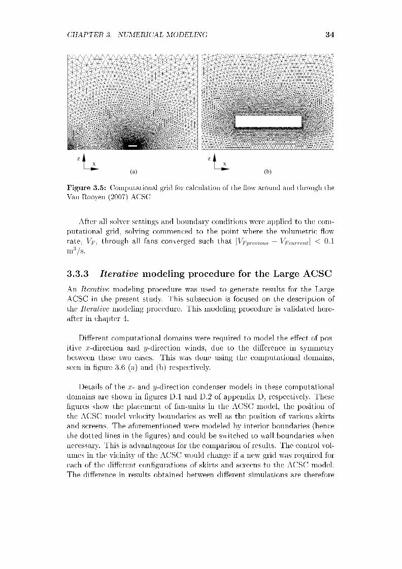
CHAPTER 3. NUMERICAL MODELING 34
Figure 3.5: Computational grid for calculation of the �ow around and through theVan Rooyen (2007) ACSC
After all solver settings and boundary conditions were applied to the com-putational grid, solving commenced to the point where the volumetric �owrate, 𝑉𝐹 , through all fans converged such that ∣𝑉𝐹𝑝𝑟𝑒𝑣𝑖𝑜𝑢𝑠 − 𝑉𝐹𝑐𝑢𝑟𝑟𝑒𝑛𝑡∣ < 0.1m3/s.
3.3.3 Iterative modeling procedure for the Large ACSC
An Iterative modeling procedure was used to generate results for the LargeACSC in the present study. This subsection is focused on the description ofthe Iterative modeling procedure. This modeling procedure is validated here-after in chapter 4.
Di�erent computational domains were required to model the e�ect of pos-itive 𝑥-direction and 𝑦-direction winds, due to the di�erence in symmetrybetween these two cases. This was done using the computational domains,seen in �gure 3.6 (a) and (b) respectively.
Details of the 𝑥- and 𝑦-direction condenser models in these computationaldomains are shown in �gures D.1 and D.2 of appendix D, respectively. These�gures show the placement of fan-units in the ACSC model, the position ofthe ACSC model velocity boundaries as well as the position of various skirtsand screens. The aforementioned were modeled by interior boundaries (hencethe dotted lines in the �gures) and could be switched to wall boundaries whennecessary. This is advantageous for the comparison of results. The control vol-umes in the vicinity of the ACSC would change if a new grid was required foreach of the di�erent con�gurations of skirts and screens to the ACSC model.The di�erence in results obtained between di�erent simulations are therefore

CHAPTER 3. NUMERICAL MODELING 35
Figure 3.6: Computational domains for calculation of the �ow around and throughthe Large ACSC by means of the Iterative modeling procedure for a (a) positive𝑥-direction and (b) positive 𝑦-direction wind
purely due to the e�ect of the mentioned modi�cations.
The grid for both the positive 𝑥- and 𝑦-direction wind domains consist of8.3(10)6 and 11.8(10)6 tetrahedral control volumes respectively. Once againthe volumes are concentrated around the ACSC model and grow larger towardthe domain outer boundaries. The grid on the symmetry plane of the posi-tive 𝑥- and 𝑦-direction domains are shown respectively in �gure 3.7 (a) and (b).
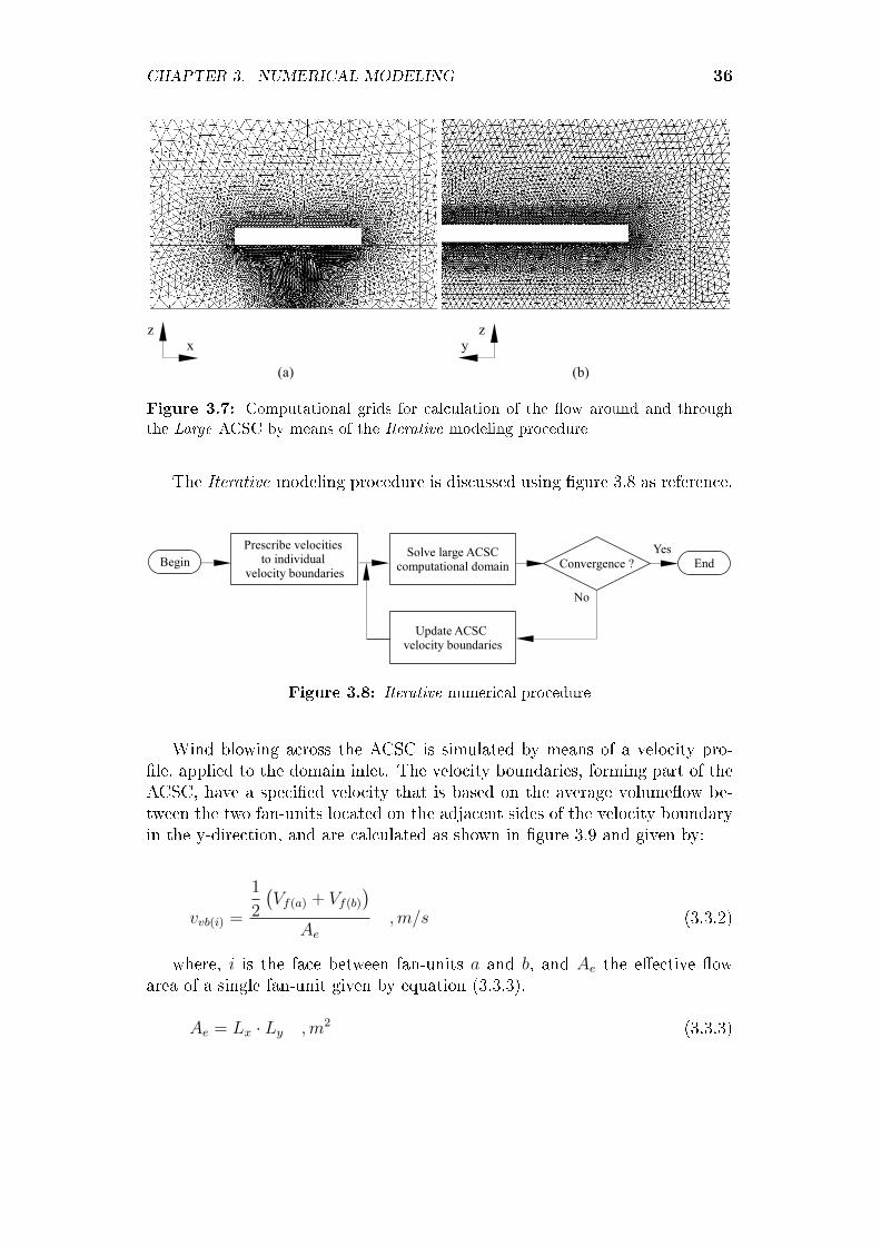
CHAPTER 3. NUMERICAL MODELING 36
Figure 3.7: Computational grids for calculation of the �ow around and throughthe Large ACSC by means of the Iterative modeling procedure
The Iterative modeling procedure is discussed using �gure 3.8 as reference.
Figure 3.8: Iterative numerical procedure
Wind blowing across the ACSC is simulated by means of a velocity pro-�le, applied to the domain inlet. The velocity boundaries, forming part of theACSC, have a speci�ed velocity that is based on the average volume�ow be-tween the two fan-units located on the adjacent sides of the velocity boundaryin the y-direction, and are calculated as shown in �gure 3.9 and given by:
𝑣𝑣𝑏(𝑖) =
1
2
(𝑉𝑓(𝑎) + 𝑉𝑓(𝑏)
)𝐴𝑒
,𝑚/𝑠 (3.3.2)
where, 𝑖 is the face between fan-units 𝑎 and 𝑏, and 𝐴𝑒 the e�ective �owarea of a single fan-unit given by equation (3.3.3).
𝐴𝑒 = 𝐿𝑥 ⋅ 𝐿𝑦 ,𝑚2 (3.3.3)

CHAPTER 3. NUMERICAL MODELING 37
Figure 3.9: Depiction of scheme used to calculate the velocity through velocityboundaries in the ACSC model
where 𝐿𝑥 and 𝐿𝑦 are given in table 3.1.
Velocities, based on ideal �ow conditions through a single fan-unit, are ap-plied to the velocity boundaries in the ACSC as a �rst approximation. Uponconvergence of the volume �ow through all individual fan-units, another simu-lation is done where the velocities through the velocity boundaries are updatedfor a next simulation. This process was then repeated until the volume �owthrough individual fans between consecutive simulations have converged.
3.4 Presentation of performance results
The purpose of the present study is to investigate the performance of a con-denser. It is therefore necessary to identify sensible ways to present perfor-mance data in order to provide comparable information. This was done byquantifying performance data in two forms of a performance e�ectiveness, dis-cussed hereafter.
3.4.1 Volumetric e�ectiveness
The volumetric e�ectiveness of the �ow rate through individual fan-units isspeci�ed as
𝜀𝑉 =𝑉𝐹
𝑉𝐹𝑖𝑑
(3.4.1)
where 𝑉𝐹 and 𝑉𝐹𝑖𝑑 is the volume �ow rate through an individual fan duringoperating conditions in the ACSC and under ideal conditions respectively. Thevolumetric e�ectiveness of �ow through a fan points out locations in the ACSC

CHAPTER 3. NUMERICAL MODELING 38
where separation and through-�ow beneath the fan platform are reducing theair �ow through the fan.
The volumetric e�ectiveness of fans not modeled was determined using thelinear interpolation scheme between adjacent fan units that were modeled.This interpolation scheme is veri�ed in appendix E.
3.4.2 Heat transfer e�ectiveness
As previously mentioned, heat transfer calculation of a single fan-unit is doneusing the 𝜀-NTU method given by equation (3.4.2), where an average steamtemperature is used in the �nned tubes.
𝑄 = 𝜀𝑚𝑎𝑐𝑝𝑎(𝑇𝑠 − 𝑇𝑎𝑖) ,𝑊 (3.4.2)
Consequently a heat transfer e�ectiveness, shown in equation (3.4.3), wouldindicate the performance of a fan-unit. This performance is the amount of heattransferred to the air by a single fan unit under certain operating conditionsof the ACSC, 𝑄𝐹 , compared to ideal operating conditions, 𝑄𝐹𝑖𝑑, of a singlefan-unit.
𝜀𝑄𝐹=
𝑄𝐹
𝑄𝐹𝑖𝑑
(3.4.3)
The overall heat transfer e�ectiveness of an ACSC unit, 𝜀𝑄𝑈, can therefore
be expressed as:
𝜀𝑄𝑈=
∑𝑛𝐹
𝑖=1 𝜀𝑄𝐹 (𝑖)
𝑛𝐹
(3.4.4)
where 𝑖 accounts for the number of fan-units, 𝑛𝐹 , in a single ACSC unit.

Chapter 4
Validation of numerical analysis
Considering that the present investigation involves the �ow around an ACSClocated in an atmospheric environment, uncertainty arises regarding the e�ectof domain boundary proximity, grid density and the e�ect of turbulence modelson the �nal numerical answer. Consequently some validation is required inorder to justify the results obtained by the numerical models used in the presentstudy. This section is dedicated to the various validations that were done,providing information on the accuracy of the numerical models.
4.1 Validation of an independent fan-unit
As mentioned in chapter 3, a numerical model was used to model the �owthrough a single fan-unit. Validation of a single fan-unit was done by com-paring the analytically obtained values for the air volume �ow through thefan and the air outlet temperature leaving the fan-unit, to the computationalresults obtained for the numerical fan-unit model.
4.1.1 Volumetric �ow rate
The ideal volumetric �ow rate, 𝑉𝐹𝑖𝑑, mentioned previously is taken as theamount of �ow through a single free standing fan-unit under the design atmo-spheric conditions given in appendix A. The �ow through a single fan-unit cananalytically be calculated using the draft equation (2.3.2). This equation wasused to calculate the fan-unit resistance to �ow and is plotted in �gure 4.1 forthe fan-unit used in the Van Rooyen (2007) ACSC, but once again omitted inthe case of the Large ACSC due to con�dentiality. The intersection of the re-sistance and fan characteristic curves, presents the operating point of a singlefan-unit.
The �ow through the Van Rooyen (2007) and Large ACSC fan-units werenumerically investigated as discussed in section 3.2. A comparison between the
39

CHAPTER 4. VALIDATION OF NUMERICAL ANALYSIS 40
Figure 4.1: Operating point of a Van Rooyen (2007) fan-unit
analytical and numerical results obtained for the �ow through both fan-unitsis given in table 4.1
Table 4.1: Comparison between analytical and numerical values for the ideal volu-metric �ow operating point
𝑽𝑭𝒊𝒅,𝒎3/𝒔
System Analytical Numerical
Large ACSC 701.68 706
Van Rooyen (2007) 645.79 640
A good correlation can be seen between the analytical and numerical re-sults, showing that the fan and numerical resistance is appropriate for use inthis study.
4.1.2 Heat transfer
As mentioned previously, heat transferred by a fan-unit to the atmosphere wasmodeled by means of a UDF. The UDF would extract information from Fluentand use this to calculate the heat transfer source term as shown in appendix C.The calculation requires two sets of information to be extracted from Fluent,namely the velocity through the control volumes and the air inlet temperatureupstream of the heat-exchanger model.

CHAPTER 4. VALIDATION OF NUMERICAL ANALYSIS 41
Two methods of air inlet temperature extraction were investigated by meansof di�erent UDF's. The �rst method (UDF 1) required the temperature tobe extracted from the control volumes immediately upstream of the heat-exchanger model. The second method (UDF 2) required the air temperatureto be extracted immediately below the fan plane. A comparison between theresults obtained by these two methods is shown in �gure 4.2.
Figure 4.2: Comparison between analytically and numerically calculated fan-unitair outlet temperatures
Figure 4.2 shows a fairly large di�erence between the results obtained bythe two temperature extraction methods. For the analytical solution, ambienttemperature is taken as the air inlet temperature into the heat-exchanger. Thesame ambient temperature is therefore required as inlet condition to the numer-ical heat-exchanger model in order for these solutions to correlate. However, as�gure 4.3 shows, signi�cant numerical di�usion occurs between the volumes inand those immediately upstream of the heat-exchanger model, giving a faultyair inlet temperature to UDF 1, calculating the heat-transfer.
To mitigate this problem, UDF 1 was recon�gured to UDF 2. The lat-ter UDF extracts the air temperatures on the fan rotating plane, rendering asolution that compares relatively well with the analytical solution. The nu-merically calculated air outlet temperature given in �gure 4.2, is the averagedvalue of all the face temperatures on the outlet plane of the numerical heat-exchanger model. Figure 4.2 shows that the numerically calculated air outlettemperature deviates slightly from the analytical solution for low air �ow rates.
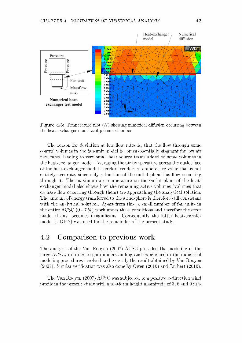
CHAPTER 4. VALIDATION OF NUMERICAL ANALYSIS 42
Figure 4.3: Temperature plot (𝐾) showing numerical di�usion occurring betweenthe heat-exchanger model and plenum chamber
The reason for deviation at low �ow rates is, that the �ow through somecontrol volumes in the fan-unit model becomes essentially stagnant for low air�ow rates, leading to very small heat source terms added to some volumes inthe heat-exchanger model. Averaging the air temperature across the outlet faceof the heat-exchanger model therefore renders a temperature value that is notentirely accurate, since only a fraction of the outlet plane has �ow occurringthrough it. The maximum air temperature on the outlet plane of the heat-exchanger model also shows how the remaining active volumes (volumes thatdo have �ow occurring through them) are approaching the analytical solution.The amount of energy transferred to the atmosphere is therefore still consistantwith the analytical solution. Apart from this, a small number of fan units inthe entire ACSC (0 - 7 %) work under these conditions and therefore the errormade, if any, becomes insigni�cant. Consequently the latter heat-transfermodel (UDF 2) was used for the remainder of the present study.
4.2 Comparison to previous work
The analysis of the Van Rooyen (2007) ACSC preceded the modeling of thelarge ACSC, in order to gain understanding and experience in the numericalmodeling procedures involved and to verify the result obtained by Van Rooyen(2007). Similar veri�cation was also done by Owen (2010) and Joubert (2010).
The Van Rooyen (2007) ACSC was subjected to a positive 𝑥-direction windpro�le in the present study with a platform height magnitude of 3, 6 and 9 m/s

CHAPTER 4. VALIDATION OF NUMERICAL ANALYSIS 43
respectively. Figure 4.4 gives a comparison of the present results obtained forthe volumetric e�ectiveness of certain fans in the Van Rooyen (2007) ACSC, tothe previous results obtained by Van Rooyen (2007), Owen (2010) and Joubert(2010).
Figure 4.4: Comparison between the numerically predicted volumetric e�ectivenessof certain fans in the Van Rooyen (2007) ACSC under positive 𝑥-direction windconditions
The results shown in �gure 4.4, generally show fair correlation. It can beseen that fans on the leading edge of the ACSC are the fans severely a�ectedby �ow distortion. This is due to separation occurring along this edge, causinga decrease in static pressure beneath edge fans as well as distorted in�ow

CHAPTER 4. VALIDATION OF NUMERICAL ANALYSIS 44
conditions. The fans further downstream are not as severely a�ected and evenhave the ability to exploit the energy in the wind, since the e�ectiveness ishigher than 1 for certain fans.
The discrepancy between the present results and those obtained by Van Rooyen(2007), Owen (2010) and Joubert (2010) could be due to a number of reasons:
Firstly, the actuator-disk fan model was used by Van Rooyen (2007), whereasthe pressure-jump method was used for fan modeling in the present study aswell as the studies conducted by Owen (2010) and Joubert (2010). Both thesemodels give an inaccurate prediction the fan performance under highly dis-torted in�ow conditions (Van der Spuy et al., 2009) and therefore some di�er-ences occur in the results obtained, especially for the edge fans. Secondly, themodeling procedure used in the present study is similar to Joubert (2010), butdi�erent from the studies of Van Rooyen (2007) and Owen (2010). Thirdly, atetrahedral grid was used in the present study, whereas a structured hexahe-dral grid was used by Van Rooyen (2007) and unstructured hexahedral grids byOwen (2010) and Joubert (2010). The results obtained using di�erent shapesof control volumes di�er due control volume skewness and density.
Despite the discrepancies in volume �ow rates through individual fans,the overall ACSC performance compares very well with that obtained byVan Rooyen (2007), Owen (2010) and Joubert (2010). A comparison betweenthe various performances calculated for the Van Rooyen (2007) ACSC undera positive 𝑥-direction wind condition can be seen in �gure 4.5.
Figure 4.5: Comparison between the numerically predicted heat-transfer e�ective-ness of the Van Rooyen (2007) ACSC under positive 𝑥-direction wind conditions

CHAPTER 4. VALIDATION OF NUMERICAL ANALYSIS 45
4.3 Sensitivity analysis
A sensitivity analysis of the computational domain used in the Iterative mod-eling procedure was done to investigate the e�ect of boundary proximity tothe ACSC model and to verify the computational accuracy of the grid. Forthis purpose three cases were individually investigated for a 3, 6 and 9 m/spositive 𝑥-direction wind and will be discussed hereafter.
Case 1 is referred to as the original case and is the analysis of the positive𝑥-direction wind grid discussed in section 3.3.
Case 2 is similar to the original case with the distinction of a larger (dimen-sional) computational domain, but the grid size in the vicinity of theACSC model remained the same as discussed in subsection 4.3.1.
Case 3 is similar to the original case in that the computational domain re-mained the same size (dimensional), but the grid is re�ned in the vicinityof the ACSC model as discussed in subsection 4.3.2 hereafter.
4.3.1 Boundary proximity
The ACSC is placed in an atmospheric environment, which is in�nitely largecompared to the ACSC. This poses the question of what the su�cient size(volumetric) of the computational domain should be in order to simulate theatmosphere.
Figure 4.6: Dimensional adjustment to the positive 𝑥-direction wind computationaldomain

CHAPTER 4. VALIDATION OF NUMERICAL ANALYSIS 46
The boundary proximity of the computational domain were adjusted asshown in �gure 4.6 to investigate the e�ect of a larger domain. After theanalysis of the larger domain, the heat-transfer e�ectiveness was calculatedfor units 1, 2 and 3 and compared to the original case as shown in �gure 4.7.Generally, good correlation can be seen, however some deviation of the originalresults occur for unit 1 and a 3 m/s wind. This error is still within �ve percentof the original value. It is therefore assumed that the dimensions of the original(case 1) computational domain is adequate since this error is marginal for thepurpose of a trend analysis.
4.3.2 Grid density
The control volumes in the entire domain were re�ned especially in the vicinityof the ACSC, since it is expected that the most distorted �ow will occur inthis region and therefore a good grid density is important. The original andadjusted cell count is given in table 4.2.
Table 4.2: Cell count of the original and adjusted computational grid
Computational domain Cell count
Large ACSC (original) 8.25(10)6
Large ACSC (re�ned) 11.87(10)6
Once again, a comparison of the heat-transfer e�ectiveness for units 1, 2and 3 at the mentioned wind speeds is illustrated in �gure 4.7. Good cor-relation between cases 1 and 3 is seen for all ACSC units, proving that thegrid density of the original (case 1) computational domain is adequate for thepresent numerical analysis.
4.4 Convergence
Two measures of convergence were monitored in the present study, namely theconvergence of �ow through individual fans in a single simulation as well theconvergence of �ow in subsequent repititions of the Iterative procedure. Thesemeasures of convergence are discussed.
4.4.1 Convergence of a single simulation
For convenience the numbering used for fans in the Large ACSC is repeatedas seen in �gure 4.8:

CHAPTER 4. VALIDATION OF NUMERICAL ANALYSIS 47
Figure 4.7: Comparison of the ACSC overall e�ectiveness for di�erent wind speedsand computational grids
Figure 4.8: Numbering of individual fans used for the Large ACSC
Computational accuracy is also obtained by allowing the numerical solutionto converge to an acceptable discrepancy. As mentioned in section 3.3, the con-vergence criterion in the present study was taken as ∣𝑉𝐹𝑝𝑟𝑒𝑣𝑖𝑜𝑢𝑠−𝑉𝐹𝑐𝑢𝑟𝑟𝑒𝑛𝑡∣ < 0.1m3/s for individual fans.
The convergence of volume �ow rate through certain fans in the �rst rowof the ACSC, for a 6 m/s positive 𝑥-direction wind, is plotted in �gure 4.9. Itshould be noted that the �ow through fans receiving three-dimensional �owconverge relatively fast compared to the fans in the two-dimensional �ow re-gion. Faster convergence of the solution was also obtained when skirts to theperiphery of and screens below the ACSC were implemented.

CHAPTER 4. VALIDATION OF NUMERICAL ANALYSIS 48
Figure 4.9: Convergence of volumetric �ow rate through certain fans in row one ofthe Large ACSC
The poor convergence in the two-dimensional region is explained by thelarge amount of separation on the upstream edge of the ACSC, but will bediscussed to more detail in chapter 5.
4.4.2 Convergence of subsequent simulations
Figure 4.10 shows the convergence of fan performance in the �rst row of theLarge ACSC, subject to a positive 𝑥-direction wind of 6 m/s. It shows a rela-tively stable convergence of the volume �ow through the fans and convergenceis obtained after two repetitions of the Iterative method.
Figure 4.10: Convergence of row 1 in the Large ACSC subject to a 6 m/s positive𝑥-direction wind obtained by the Iterative method


