Phase Field Fracture Mechanics

MAE 523 Term Paper

Brett A. Robertson

Arizona State University

Tempe, AZ, USA

November 21, 2015

Abstract

For this assignment, a newer technique of fracture mechanics using a phase field

approach, will be examined and compared with experimental data for a bend test and

a tension test.

The software being used is Sierra Solid Mechanics, an implicit/explicit finite element

code developed at Sandia National Labs in Albuquerque, New Mexico. The bend test

experimental data was also obtained at Sandia Labs while the tension test data was

found in a report online from Purdue University.

1

SAND2015-10305R

Contents

1 Background 3

2 Phase Field Formulation 4

2.1 Effect of Length Scale . . . . . . . . . . . . . . . . . . . . . . . . . . . . . . . 5

3 3 Point Bend Test 8

3.1 Model Creation . . . . . . . . . . . . . . . . . . . . . . . . . . . . . . . . . . . 8

3.2 Results . . . . . . . . . . . . . . . . . . . . . . . . . . . . . . . . . . . . . . . . 11

4 Axial Tension Test 15

4.1 Model Creation . . . . . . . . . . . . . . . . . . . . . . . . . . . . . . . . . . . 16

4.2 Results . . . . . . . . . . . . . . . . . . . . . . . . . . . . . . . . . . . . . . . . 16

5 Problems Encountered 21

5.1 Dynamics Involved with 4 Point Bend . . . . . . . . . . . . . . . . . . . . . . 21

5.2 Contact Issue with Charpy Impact Test . . . . . . . . . . . . . . . . . . . . . 22

6 Conclusions and Future Work 23

2

1 Background

As fracture mechanics plays a key role in engineering design and analysis, it is an important

topic with extensive research currently proceeding. Most methods of modeling fracture are

done using finite element method and are based off of different techniques. Several tech-

niques are based off of Griffith’s linear elastic brittle fracture, which is modeled using the

energy release rate. Essentially, once the energy release rate hits a critical value, the crack

is able to grow or propagate further. Another more recent method is the use of extended

finite element methods (XFEM). However, both of these methods treat the crack discretely.

The proposed phase field approach differs from these methods as it takes a small piece of the

crack boundary, smooths it, and then approximates the fracture surface [1] [4] [5]. It uses a

diffusive crack approach instead of modeling the discontinuities of the crack. The diffusive

crack zone is determined by a scalar variable that interpolates between either the broken

or unbroken state of the material. The phase field variable will take the value 0 inside the

crack surface and 1 away from the crack surface, therefore this variable, c, is only on the set

[0,1]. The basic scheme for using phase field fracture:

-Initialize displacement (u), fracture phase (c), and history fields (H)

-Compute maximum reference energy (H)

-Determine current fracture phase field (c)

- Compute the current displacement field (u)

Within the formulation for the phase field, there are constraints that restrict the crack from

translating, but allow it to extend, branch, and merge.

Two of the proposed benefits of this approach are that the crack no longer has to follow

3

element edges and can propagate freely and that the solution will eventually converge,

whereas with previous methods, mesh refinement will only create higher and higher stress

at the crack tip while not necessarily converging.

2 Phase Field Formulation

The current formulation for the method of phase field fracture is based off of brittle fracture.

There is, however, currently another method being developed which will also include ductile

materials. In order for this model to work, the assumption of small deformations is taken,

and strain tensor is defined as:

εij = uij =1

2(∂ui∂xj

+∂uj∂xi

)

The linear elastic energy density is:

ψe(ε) =1

2λεiiεjj + µεijεij

and the total potential energy of a body with a crack is:

Ψ =

∫Ω

ψedx+

∫Γ

Gcdx

where Ω is the body and Γ is the crack discontinuity surface.

There is a length scale parameter, l, which determines essentially the area of the crack

”smear”. This comes in as the phase field is approximated as:

c(x) = e−|x|/l

When expanding to multi-dimensional solids the phase field approximation becomes the

minimization problem:

c(x, t) = Arg

inf Γl(c)

where:

Γl(c) =

∫Ω

γdV

4

and:

γ =1

2lc2 +

l

2|∇c|2

∇c is the spatial gradient.

Going back to the fracture energy, Gc, it can be approximated as:∫Γ

Gcdx =

∫Ω

[ (c− 1)2

4l+ l

∂c

∂xi

∂c

∂xi

]dx

Once damage beings to occur, there is essentially a loss of stiffness in the material. This

loss in stiffness represents the model experiencing crack propagation and separation in the

material. This stiffness loss is limited to the failure zone and approximates the fracture

surface, which physically isn’t there because the elements do not actually break or disappear.

This loss of stiffness is input in the elastic energy and is given by:

ψe(ε, c) =[(1− k)c2 + k]ψ+

e (ε) + ψ−e (ε)]

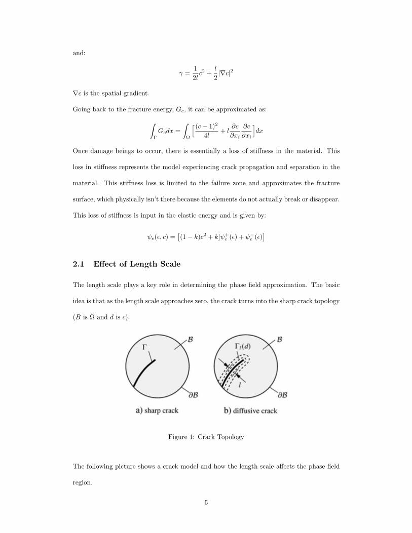
2.1 Effect of Length Scale

The length scale plays a key role in determining the phase field approximation. The basic

idea is that as the length scale approaches zero, the crack turns into the sharp crack topology

(B is Ω and d is c).

Figure 1: Crack Topology

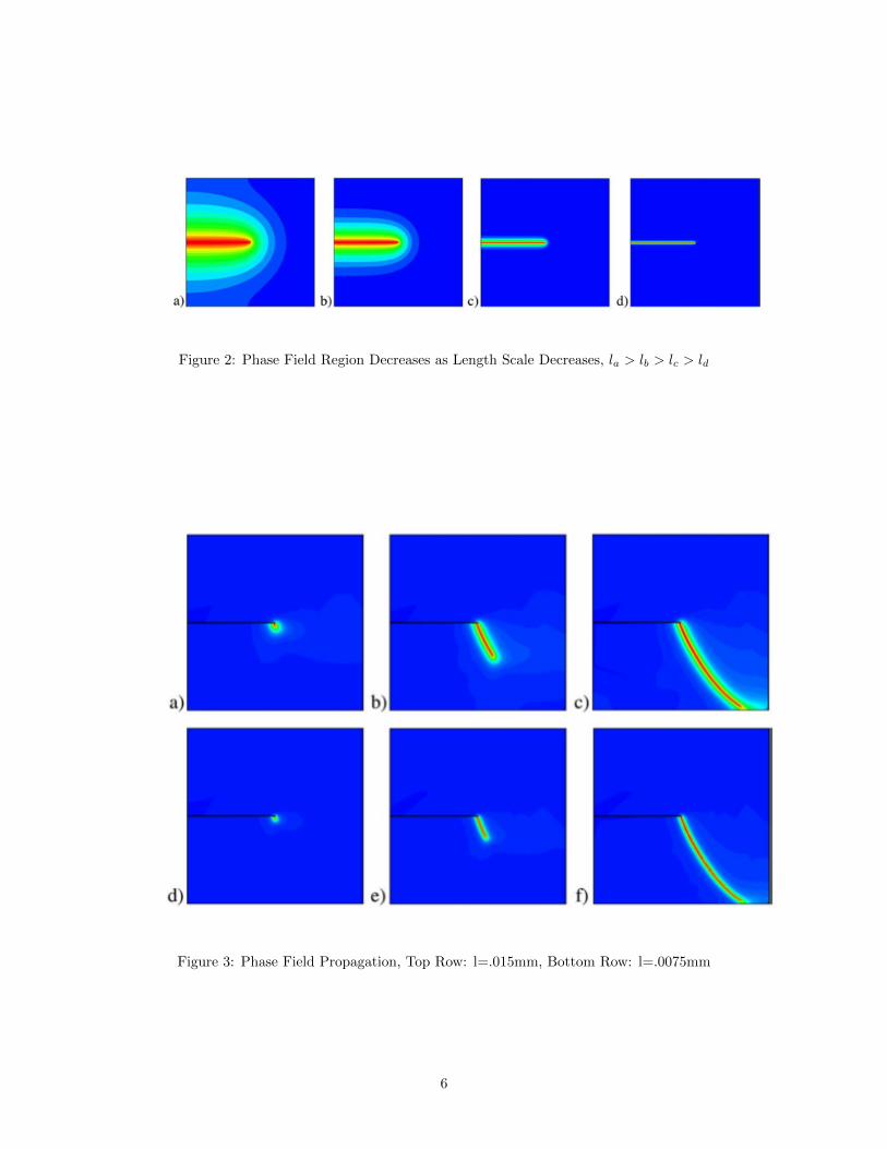
The following picture shows a crack model and how the length scale affects the phase field

region.

5

Figure 2: Phase Field Region Decreases as Length Scale Decreases, la > lb > lc > ld

Figure 3: Phase Field Propagation, Top Row: l=.015mm, Bottom Row: l=.0075mm

6

It can be seen that as the length scale is reduced to close to zero, the sharp crack topology

is almost achieved. For this project, a length scale is chosen to be approximately 2-3 times

the length of the smallest element size of the mesh.

7

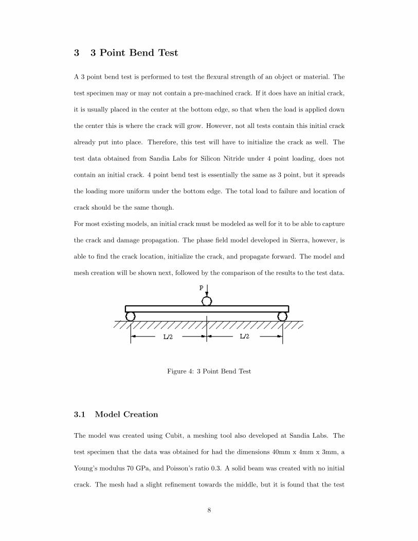
3 3 Point Bend Test

A 3 point bend test is performed to test the flexural strength of an object or material. The

test specimen may or may not contain a pre-machined crack. If it does have an initial crack,

it is usually placed in the center at the bottom edge, so that when the load is applied down

the center this is where the crack will grow. However, not all tests contain this initial crack

already put into place. Therefore, this test will have to initialize the crack as well. The

test data obtained from Sandia Labs for Silicon Nitride under 4 point loading, does not

contain an initial crack. 4 point bend test is essentially the same as 3 point, but it spreads

the loading more uniform under the bottom edge. The total load to failure and location of

crack should be the same though.

For most existing models, an initial crack must be modeled as well for it to be able to capture

the crack and damage propagation. The phase field model developed in Sierra, however, is

able to find the crack location, initialize the crack, and propagate forward. The model and

mesh creation will be shown next, followed by the comparison of the results to the test data.

Figure 4: 3 Point Bend Test

3.1 Model Creation

The model was created using Cubit, a meshing tool also developed at Sandia Labs. The

test specimen that the data was obtained for had the dimensions 40mm x 4mm x 3mm, a

Young’s modulus 70 GPa, and Poisson’s ratio 0.3. A solid beam was created with no initial

crack. The mesh had a slight refinement towards the middle, but it is found that the test

8

results are mostly mesh independent, so no extreme refinement needed to be performed.

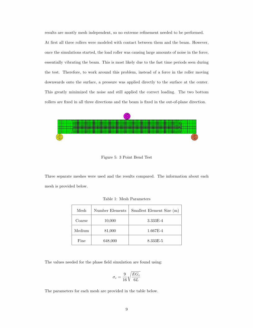
At first all three rollers were modeled with contact between them and the beam. However,

once the simulations started, the load roller was causing large amounts of noise in the force,

essentially vibrating the beam. This is most likely due to the fast time periods seen during

the test. Therefore, to work around this problem, instead of a force in the roller moving

downwards onto the surface, a pressure was applied directly to the surface at the center.

This greatly minimized the noise and still applied the correct loading. The two bottom

rollers are fixed in all three directions and the beam is fixed in the out-of-plane direction.

Figure 5: 3 Point Bend Test

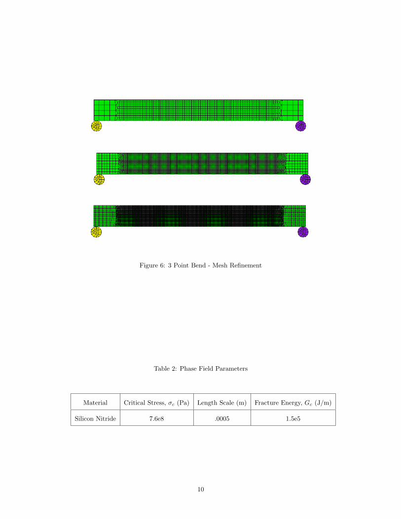
Three separate meshes were used and the results compared. The information about each

mesh is provided below.

Table 1: Mesh Parameters

Mesh Number Elements Smallest Element Size (m)

Coarse 10,000 3.333E-4

Medium 81,000 1.667E-4

Fine 648,000 8.333E-5

The values needed for the phase field simulation are found using:

σc =9

16

√EGc

6L

The parameters for each mesh are provided in the table below.

9

Figure 6: 3 Point Bend - Mesh Refinement

Table 2: Phase Field Parameters

Material Critical Stress, σc (Pa) Length Scale (m) Fracture Energy, Gc (J/m)

Silicon Nitride 7.6e8 .0005 1.5e5

10

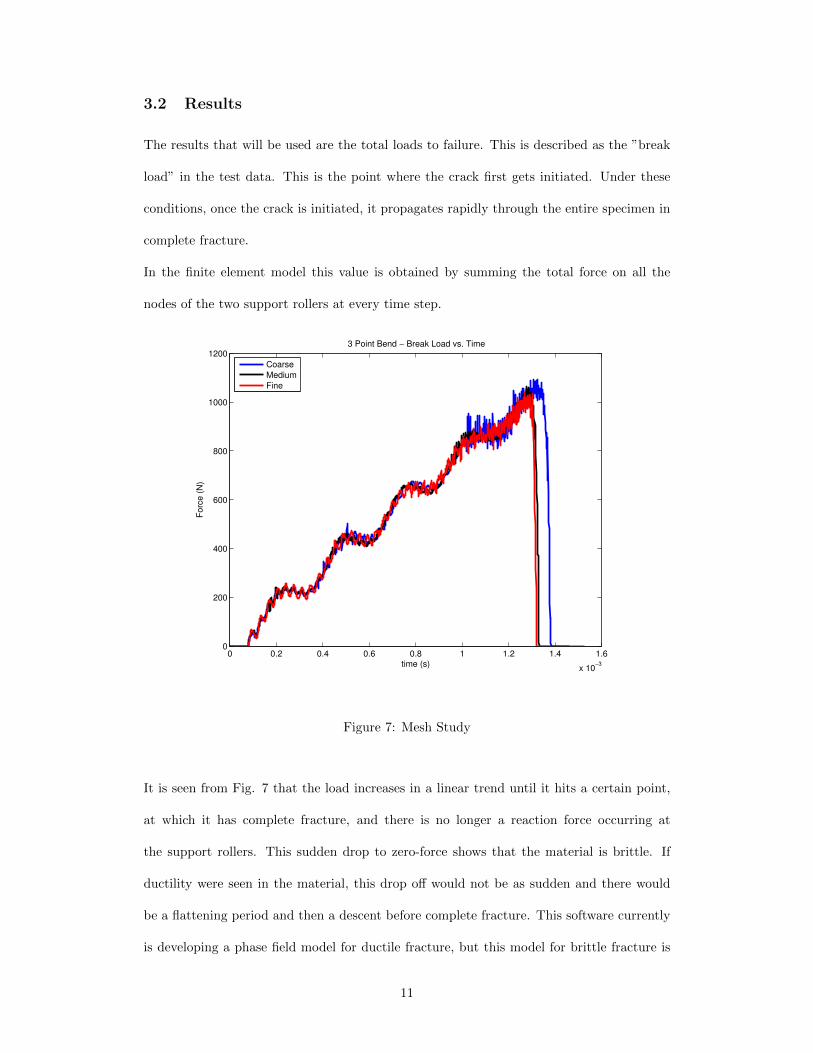
3.2 Results

The results that will be used are the total loads to failure. This is described as the ”break

load” in the test data. This is the point where the crack first gets initiated. Under these

conditions, once the crack is initiated, it propagates rapidly through the entire specimen in

complete fracture.

In the finite element model this value is obtained by summing the total force on all the

nodes of the two support rollers at every time step.

0 0.2 0.4 0.6 0.8 1 1.2 1.4 1.6

x 10−3

0

200

400

600

800

1000

1200

time (s)

Forc

e (

N)

3 Point Bend − Break Load vs. Time

Coarse

Medium

Fine

Figure 7: Mesh Study

It is seen from Fig. 7 that the load increases in a linear trend until it hits a certain point,

at which it has complete fracture, and there is no longer a reaction force occurring at

the support rollers. This sudden drop to zero-force shows that the material is brittle. If

ductility were seen in the material, this drop off would not be as sudden and there would

be a flattening period and then a descent before complete fracture. This software currently

is developing a phase field model for ductile fracture, but this model for brittle fracture is

11

the only one available.

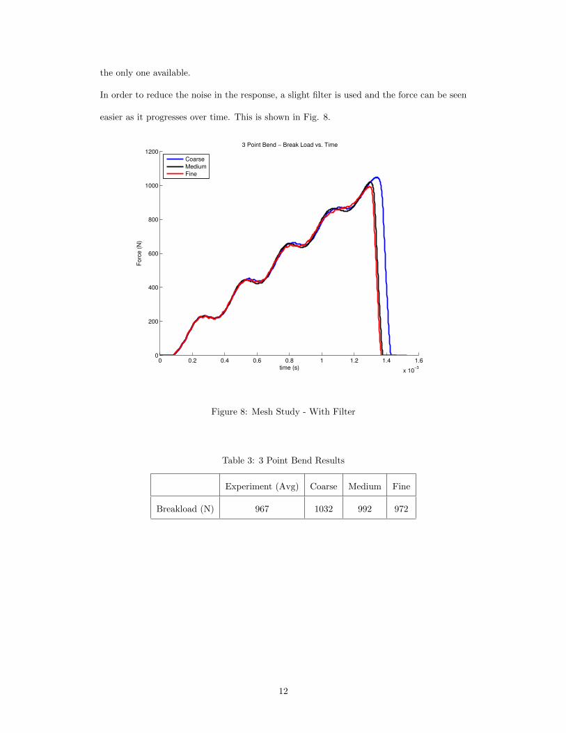
In order to reduce the noise in the response, a slight filter is used and the force can be seen

easier as it progresses over time. This is shown in Fig. 8.

0 0.2 0.4 0.6 0.8 1 1.2 1.4 1.6

x 10−3

0

200

400

600

800

1000

1200

time (s)

Forc

e (

N)

3 Point Bend − Break Load vs. Time

Coarse

Medium

Fine

Figure 8: Mesh Study - With Filter

Table 3: 3 Point Bend Results

Experiment (Avg) Coarse Medium Fine

Breakload (N) 967 1032 992 972

12

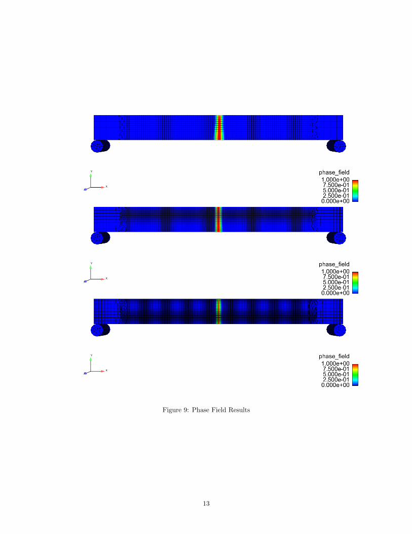
Figure 9: Phase Field Results

13

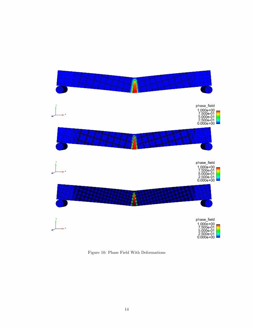
Figure 10: Phase Field With Deformations

14

4 Axial Tension Test

In order to further test the phase field fracture method on brittle materials, a Double Edge

Notch Tension (DENT) test is modeled. Test data was found online in a school report that

performed the test on both ductile and brittle steel [2]. The model will be compared to the

results of the brittle test. A tension test like this is very common in engineering and materials

science to understand how material behave under pure tension. The experiment performed

was under displacement control of .002 in/min. The material used in the experiment is 1090

cold drawn and annealed brittle steel.

Figure 11: Axial Tension Test

15

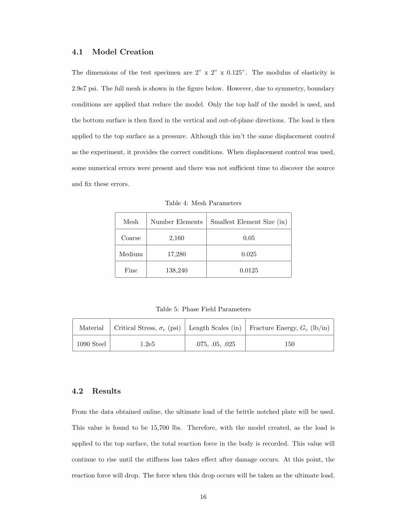
4.1 Model Creation

The dimensions of the test specimen are 2” x 2” x 0.125”. The modulus of elasticity is

2.9e7 psi. The full mesh is shown in the figure below. However, due to symmetry, boundary

conditions are applied that reduce the model. Only the top half of the model is used, and

the bottom surface is then fixed in the vertical and out-of-plane directions. The load is then

applied to the top surface as a pressure. Although this isn’t the same displacement control

as the experiment, it provides the correct conditions. When displacement control was used,

some numerical errors were present and there was not sufficient time to discover the source

and fix these errors.

Table 4: Mesh Parameters

Mesh Number Elements Smallest Element Size (in)

Coarse 2,160 0.05

Medium 17,280 0.025

Fine 138,240 0.0125

Table 5: Phase Field Parameters

Material Critical Stress, σc (psi) Length Scales (in) Fracture Energy, Gc (lb/in)

1090 Steel 1.2e5 .075, .05, .025 150

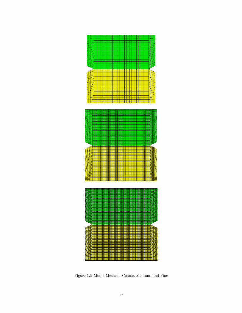
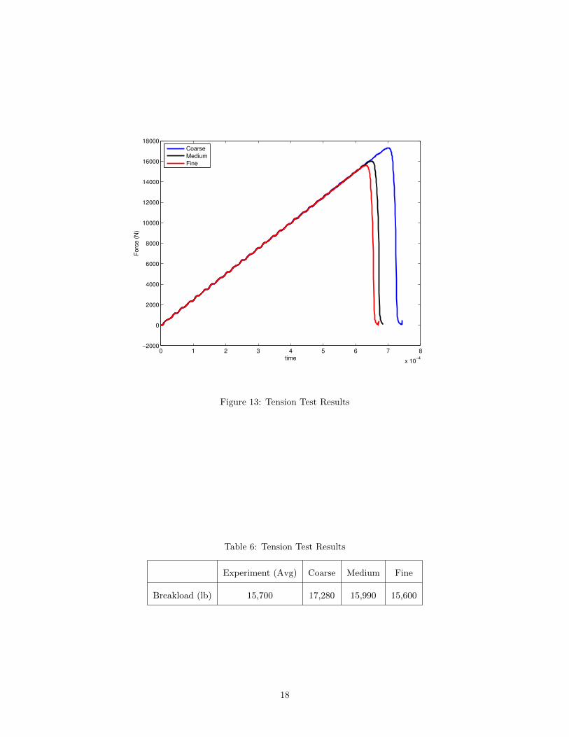
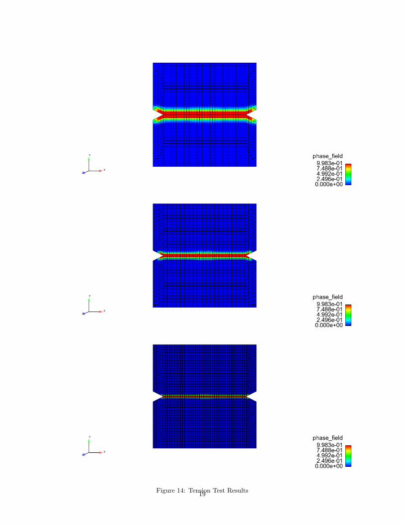
4.2 Results

From the data obtained online, the ultimate load of the brittle notched plate will be used.

This value is found to be 15,700 lbs. Therefore, with the model created, as the load is

applied to the top surface, the total reaction force in the body is recorded. This value will

continue to rise until the stiffness loss takes effect after damage occurs. At this point, the

reaction force will drop. The force when this drop occurs will be taken as the ultimate load.

16

Figure 12: Model Meshes - Coarse, Medium, and Fine

17

0 1 2 3 4 5 6 7 8

x 10−4

−2000

0

2000

4000

6000

8000

10000

12000

14000

16000

18000

time

Fo

rce

(N

)

Coarse

Medium

Fine

Figure 13: Tension Test Results

Table 6: Tension Test Results

Experiment (Avg) Coarse Medium Fine

Breakload (lb) 15,700 17,280 15,990 15,600

18

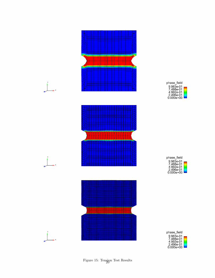
Figure 14: Tension Test Results19

Figure 15: Tension Test Results20

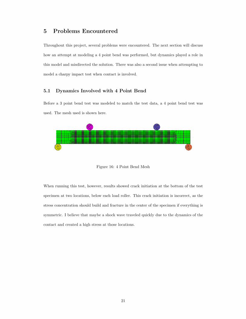
5 Problems Encountered

Throughout this project, several problems were encountered. The next section will discuss

how an attempt at modeling a 4 point bend was performed, but dynamics played a role in

this model and misdirected the solution. There was also a second issue when attempting to

model a charpy impact test when contact is involved.

5.1 Dynamics Involved with 4 Point Bend

Before a 3 point bend test was modeled to match the test data, a 4 point bend test was

used. The mesh used is shown here.

Figure 16: 4 Point Bend Mesh

When running this test, however, results showed crack initiation at the bottom of the test

specimen at two locations, below each load roller. This crack initiation is incorrect, as the

stress concentration should build and fracture in the center of the specimen if everything is

symmetric. I believe that maybe a shock wave traveled quickly due to the dynamics of the

contact and created a high stress at those locations.

21

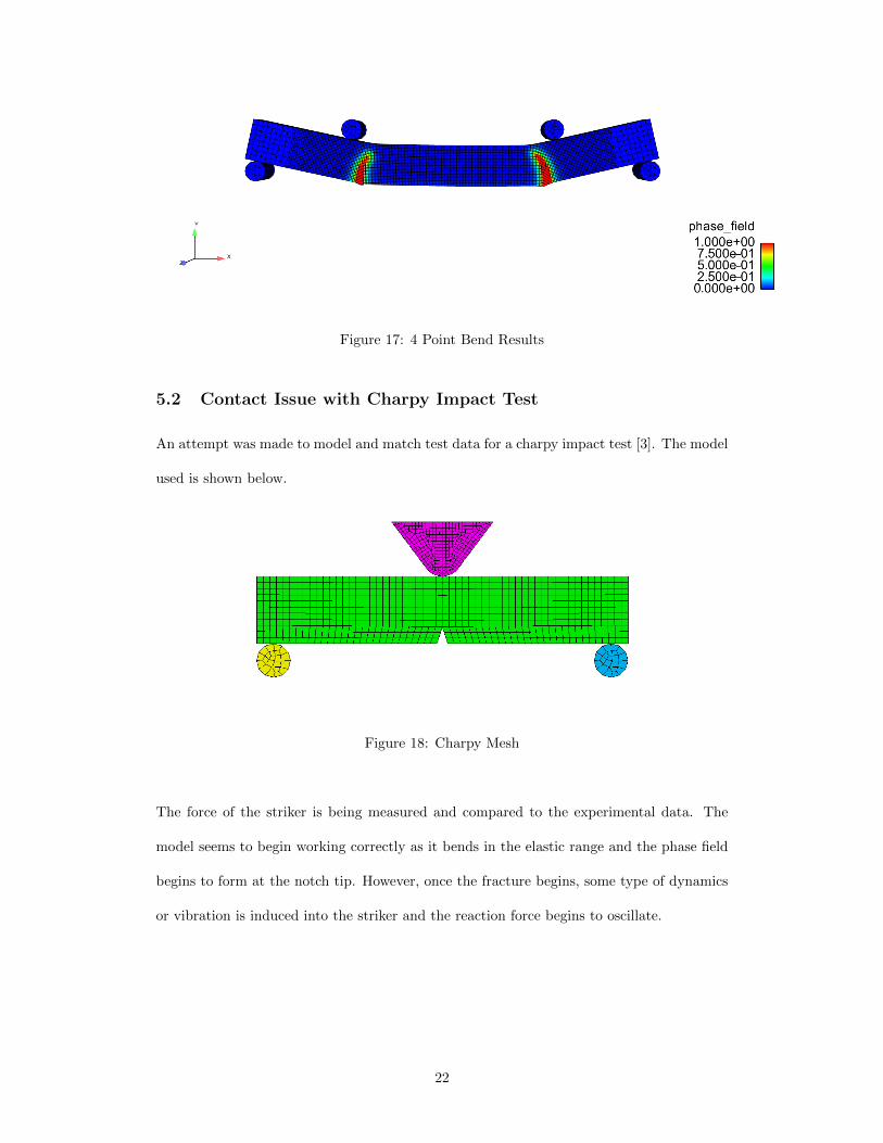
Figure 17: 4 Point Bend Results

5.2 Contact Issue with Charpy Impact Test

An attempt was made to model and match test data for a charpy impact test [3]. The model

used is shown below.

Figure 18: Charpy Mesh

The force of the striker is being measured and compared to the experimental data. The

model seems to begin working correctly as it bends in the elastic range and the phase field

begins to form at the notch tip. However, once the fracture begins, some type of dynamics

or vibration is induced into the striker and the reaction force begins to oscillate.

22

0.5 1 1.5 2 2.5 3

x 10−3

0

2000

4000

6000

8000

10000

12000

14000

16000

time

Fo

rce

(N

)

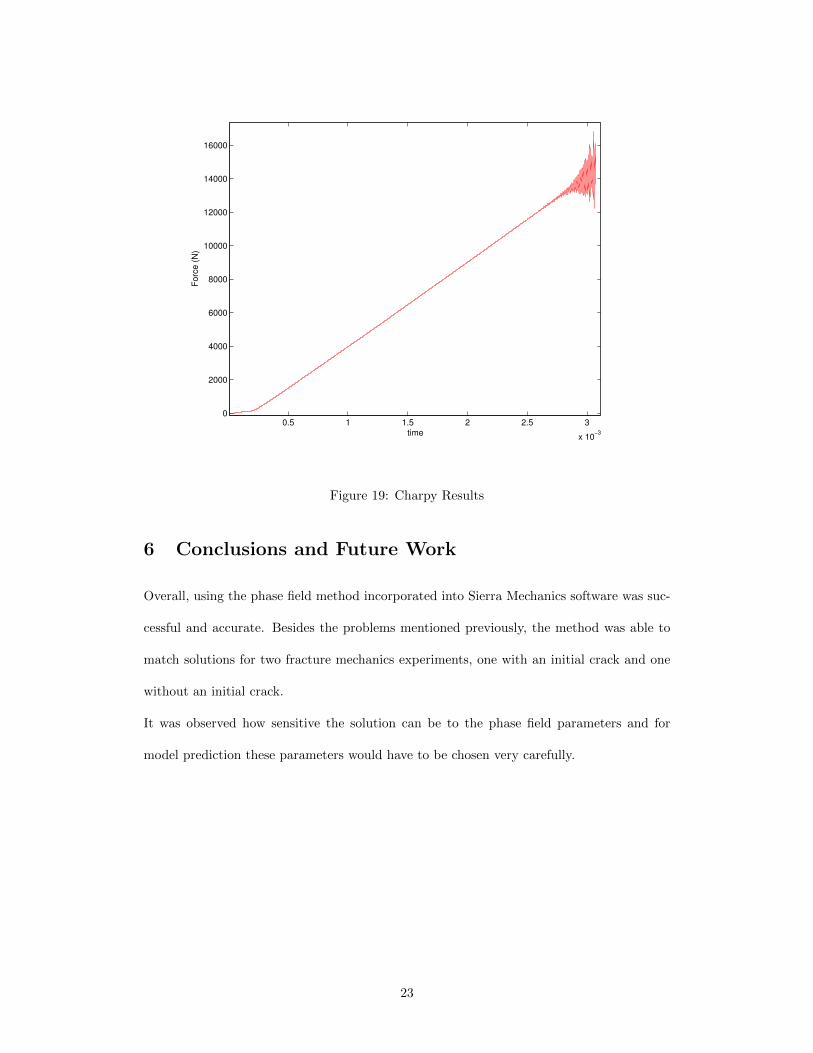
Figure 19: Charpy Results

6 Conclusions and Future Work

Overall, using the phase field method incorporated into Sierra Mechanics software was suc-

cessful and accurate. Besides the problems mentioned previously, the method was able to

match solutions for two fracture mechanics experiments, one with an initial crack and one

without an initial crack.

It was observed how sensitive the solution can be to the phase field parameters and for

model prediction these parameters would have to be chosen very carefully.

23

References

[1] M.J. Borden, C.V. Verhoosel, M.A. Scott, T.J.R. Hughes, and C.M. Landis. A phase-field

discription of dynamic brittle fracture. Technical report, Institute for Computational

Engineering and Sciences, The University of Texas at Austin, 2011.

[2] M. Choi, T. Kim, and C. Villani. Fracture toughness test and its simulation for brittle

and ductile steel. Technical report, Purdue University, 2011.

[3] S.H. Hashemi, I.C. Howard, J.R. Yates, and R.M. Andrews. Measurement and analysis

of impact test data for x100 pipeline steel. Applied Mechanics and Materials, 3-4, 2005.

[4] E. Lorentz, S. Cuvilliez, and K. Kazymyrenko. Convergence of a gradient damage model

toward a cohesive zone model. Comptes Rendus Mecanique, 339, 2011.

[5] C. Miehe, M. Hofacker, and F. Welschinger. A phase field model for rate-independent

crack propagation: Robust algorithmic implementation based on operator splits. Com-

puter Methods in Applied Mechanics and Engineering, 199, 2010.

24