Page 1
Design, Simulation and Implementation of
a PMSM Drive System
Thesis for the Degree of Master of Science in Engineering
DAVID VINDEL MUÑOZ
Division of Electric Power Engineering Department of Energy and Environment Chalmers University of Technology
Göteborg, Sweden 2011
Page 3
Thesis for the Degree of Master of Science in Engineering
DAVID VINDEL MUÑOZ
Division of Electric Power Engineering Department of Energy and Environment
Chalmers University of Technology
Göteborg, Sweden 2011
Page 4
Design, Simulation and Implementation of a PMSM Drive System
Thesis for the Degree of Master of Science in Engineering
DAVID VINDEL MUÑOZ
© DAVID VINDEL MUÑOZ, 2011
Division of Electric Power Engineering Department of Energy and Environment Chalmers University of Technology
SE-412 96 Göteborg
Sweden
Telephone: + 46 (0)31-772 1000
Cover:
Picture of the experimental drive system setup
Chalmers Bibliotek, Reproservice
Göteborg, Sweden 2011
Page 5
I
Acknowledgments
In first place, I wish to express my gratitude to Saeid Haghbin, the person that gave
me the opportunity to carry out such a challenging project. His guidance, help and
technical support throughout these months have been essential.
Also thank to Ola Carlson and the division of Electric Power Engineering, within the
department of Energy and Environment, for this academic experience in Chalmers
University of Technology.
During the development of the thesis, some problems arose and some help was
needed. In this section, apart from Saeid, I have to declare an immense gratitude to
Stefan Lundberg, Massimo Bongiorno and Robert Karlsson.
A special mention to all the friends I met here in Sweden and have shared such a great
year. Frölunda People, as a family, Högsbogatians always there and Masthugget BK,
the unexpected surprise. Extraordinary year!
Somehow, I have to express here my acknowledgement to so many people in Spain.
To all these special people, with whom I have spent my life, thanks for all the
unforgettable moments we have lived together.
Finally, thank my family because they make this real. An entire life support is
priceless. Love you Padres!
Göteborg, May 2011
David Vindel Muñoz
Page 7
III
Design, Simulation and Implementation of a PMSM Drive System
Thesis for the Degree of Master of Science in Engineering
DAVID VINDEL MUÑOZ Division of Electric Power Engineering Department of Energy and Environment
Chalmers University of Technology
ABSTRACT
Field oriented control (FOC) of permanent magnet synchronous motor (PMSM) is one
of the widely used methods for the speed control of the motor. A PMSM drive system
based on FOC is designed, simulated and implemented.
The whole drive system is simulated in Matlab/Simulink based on the mathematical
model of the system devices including PMSM and inverter. The aim of the drive
system is to have speed control over wide speed range. Simulation results show that
the speed controller has a good dynamic response.
A lab setup is designed and implemented based on a six-pole 2 kW PMSM. The
measurement devices, voltage transducers, current transducers and resolver, are
explained in this report. For the system control dSpace is used and Matlab/Simulink is
used for the program development and implementation.
Experimental results show that the drive system has a good dynamic response in terms
of speed response and torque ripple. The drive system will be extended to serve as an
isolated high power battery charger.
Key words: PMSM, FOC, Drive System, Isolated Charger.
Page 9
V
Table of Contents
ACKNOWLEDGMENTS I
ABSTRACT III
TABLE OF CONTENTS V
1 INTRODUCTION 1
1.1 Background of the study 1
1.2 Objectives of the study 1
1.3 Outline of the thesis 1
2 MODELLING AND FIELD ORIENTED CONTROL OF PERMANENT
MAGNET SYNCHRONOUS MACHINE 2
2.1 Mathematical model of PMSM 2
2.2 Field oriented control of PMSM 5
2.3 Simulation results 9
3 PRACTICAL IMPLEMENTATION OF A PMSM DRIVE SYSTEM 16
3.1 General hardware overview 16
3.2 PMSM 19
3.3 Inverter 20
3.4 Measurement interfaces 21
3.4.1 Voltage measurements 22 3.4.2 Current measurements 25 3.4.3 Position and speed measurements 26
3.5 Connection to the grid By a relay 29
3.6 dSpace system 30
3.7 Experimental results 33
4 CONCLUSIONS AND FUTURE WORK 36
4.1 Conclusions 36
4.2 Future work 36
REFERENCES 37
APPENDICES 38
Page 10
Appendix A. Reference frame conversion 38
Appendix B. Matlab code and Simulink block diagrams 40
Appendix C. Lab setup diagrams 45
Appendix D. Data sheet of experimental equipments 49
Appendix E. dSpace software implementation 72
Page 13
CHALMERS, Energy and Environment, Master´s Thesis
1
1 Introduction
The project background, objective of the project and the thesis outline is described in
this introductory chapter.
1.1 Background of the study
Many types of electric motors have been used in the industry for different purposes:
cranes, spinning machines, public transportation and so on [3]. AC motors are widely
used and ac drives are subject of study for many researchers [4, 13]. Recently, ac
drives in vehicle applications are gaining attention due to pollution and fuel price
problems.
In the electrical system of an electric or hybrid electric vehicle based on an ac motor,
the motor is producing torque from the battery through the inverter. To charge the
battery the grid power is utilized in some vehicles called grid-connected version.
Since the battery charging and traction power is not happening simultaneously it is
possible to use inverter and motor in charger circuit to reduce the price, volume,
weight and space of the charger. This is called integrated charger.
An isolated high power integrated charger is proposed in [9] that is based on a special
ac motor winding configuration. To implement a practical system of the proposed
integrated charger, this current subproject is defined to be extended later on.
1.2 Objectives of the study
The goal of this thesis is to design and implement a normal drive system of a
permanent magnet synchronous machine (PMSM). The stator has double set of
winding as explained in [12]. Later on the system will be used as an integrated
charger.
The drive system simulation and the hardware implementation is explained in this
thesis.
The simulations are conducted in Matlab/Simulink software. Based on the simulation
results, a practical system is designed and implemented that is explained in the report.
dSpace control system is used to control the whole drive system.
1.3 Outline of the thesis
After this introduction chapter, the mathematical model of PMSM and the field
oriented method is explained in chapter 2. Chapter 3 includes design and description
of the practical system. Conclusion and future works are presented in chapter 4.
Several appendices are added to the report as a part of the thesis. Reference frame
theory, Matlab code used for the simulations, as well as the Simulink blocks of every
subsystem, the lab setup diagrams and components datasheets and dSpace
programming are presented in appendices.
Page 14
2 CHALMERS, Energy and Environment, Master’s Thesis
2 Modelling and field oriented control of permanent
magnet synchronous machine
Permanent magnet synchronous motors (PMSM) have attracted increasing interest in
recent years for industrial drive applications [3]. The high efficiency, high steady state
torque density and simple controller of the PM motor drives compared to the
induction motor drives make them a good alternative in certain applications.
Other advantages of the PMSM are low inertia, high efficiency, reliability and low
cost of the power electronic converters required for controlling the machine [1]. All
these facts make the PMSM an excellent candidate for being used in many
applications.
We can distinguish between two main kinds of PMSM: internal-mounted magnets
(with saliency, IM) or surface-mounted magnets (without saliency, SM). The main
difference is that the IM machine has a variable reluctance which varies with the rotor
angle, while the SM machine has quite a fixed reluctance for any rotor angle. That
leads in a uniform air gap, and thus, an equal magnetizing inductance for the direct
and quadrature axis (Ld and Lq) [2].
Field oriented control of PMSM is one of the widely used methods in drive
applications [14] that is considered in this thesis. A mathematical model of PMSM is
introduced in this chapter first. Then the FOC method is explained. Finally
Matlab/Simulink based simulation results are presented for this scheme.
2.1 Mathematical model of PMSM
A surface-mounted synchronous machine is used in this project, so the mathematical
model of the PMSM is presented for this kind of machine.
Figure 2.1 show a cross section of the rotor and stator of a PMSM.
Page 15
CHALMERS, Energy and Environment, Master´s Thesis
3
Figure 2.1: View of a three phase, two-pole PMSM.
Considering a two-pole three phase PMSM, the voltage equation in the dq domain
(reference frame transformation is explained in Appendix A. Reference frame
conversion) is expressed as follows [2]:
(2.1)
Where p is the differentiating operator . The indexes d, q and 0 denote direct
axis, quadrature axis and zero component of the variables respectively. The flux
linkage in the dq frame can be calculated as follows:
(2.2)
Where the inductance matrix is expressed:
(2.3)
Page 16
4 CHALMERS, Energy and Environment, Master’s Thesis
For SMPM, the d and q components of the inductances are the same. The notation dq
is change for s, which refers to the stator. The magnetizing flux has the following
expression:
(2.4)
A usual way to write the equation (2.1) is in its expanded form. As far as the stator
windings are wye-connected (with a neutral point) and supplied with balanced three
phase currents, the zero-axis components are neglected [2]. The voltage equations for
d and q axes are:
(2.5)
(2.6)
Where Rs is the stator resistance, Ls the stator inductance, ωr the rotor rotational speed
and λpm the permanent magnet flux.
The electromagnetic torque of the machine can be expressed, in the dq reference
frame, as follows:
(2.7)
If the equation (2.2) is substituted in the torque equation, it is obtained:
(2.8)
Considering a non-salient rotor, where the inductances are equal, the final expression
of the electromagnetic torque is:
(2.9)
This result is quite interesting. It shows that the only component involved in torque
production in a PMSM without saliency is the stator q-axis current.
Page 17
CHALMERS, Energy and Environment, Master´s Thesis
5
2.2 Field oriented control of PMSM
Field oriented control of PMSM is one important variation of vector control methods
[14]. The aim of the FOC method is to control the magnetic field and torque by
controlling the d and q components of the stator currents or relatively fluxes.
With the information of the stator currents and the rotor angle a FOC technique can
control the motor torque and the flux in a very effective way. The main advantages of
this technique are the fast response and the little torque ripple [5].
The implementation of this technique will be carried out using two current regulators,
one for the direct-axis component and another for the quadrature-axis component, and
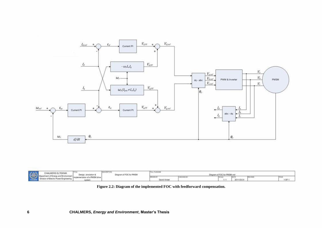
one speed regulator. Figure 2.2 shows a block diagram of the FOC method.
Page 18
6 CHALMERS, Energy and Environment, Master’s Thesis
Figure 2.2: Diagram of the implemented FOC with feedforward compensation.
Page 19
CHALMERS, Energy and Environment, Master´s Thesis
7
As shown in the figure, there are three PI regulators in the control system. One is for
the mechanical system (speed) and two are for the electrical system (d and q currents).
At first, the reference speed, ωref, is compared with the measured speed, ωr, and the
error signal, εω, is fed to the speed PI controller. This regulator compares the actual
and reference speed and outputs a torque command. The torque is related to the speed
by the mechanical equation of the motor:
(2.10)
Where J is the inertia of the motor, B is the viscous coefficient, Tm is the mechanical
torque applied in the shaft (load) and Te is the electrical torque developed by the
motor.
Once is obtained the torque command, with the equation (2.9) can be turned into the
quadrature-axis current reference, Iq,ref [2].
There is a PI controller to regulate the d component of the stator current. The
reference value, Id,ref, is zero in this thesis since there is no flux weakening operation.
The d component error of the current, εd, is used as an input for the PI regulator.
Moreover, there is another PI controller to regulate the q component of the current.
The reference value is compared with the measured and then fed to the PI regulator.
Feedforward compensation is used in d and q PI regulators according to equations
(2.5) and (2.6), to enhance the system performance.
The PI outputs, Vd,ref and Vq,ref, are first transformed to abc domain by the use of
inverse Park and Clark transformations (see Appendix A. Reference frame
conversion). Then, those reference voltages are used by the PWM unit to generate the
inverter‟scommandsignals.
ThetuningofthePI‟s(settingthePandIparameters)hasbeen carried out with the
following method proposed by [7].
(2.11)
(2.12)
(2.13)
(2.14)
(2.15)
(2.16)
(2.17)
(2.18)
Page 20
8 CHALMERS, Energy and Environment, Master’s Thesis
Where αcurrent amd αspeed are the controller‟s bandwith and fs is the switching
frequency of the inverter (same as the sampling frequency of the system).
All the current and speed regulators have been implemented taking care of the torque
and voltage limits. A saturation block has been included to avoid exceeding the
maximum torque and voltages allowed in the machine. When these limits are reached,
the regulators control that the torque or voltage values do not overpass their maximum
values. This causes a problem, a large overshoot of the current values caused by the
integrator windup. The integral term of the regulator keeps accumulating the error
during the time of maximum voltage output, and when the value of the current reaches
its maximum, the integrator has wound up so that the voltage remains large [7].
To prevent this problem, anti-windup technique is used in the controllers. The
reference value of torque or voltage is used to update the integral term of the
regulator. As it can be seen in the Simulink block diagram, as far as the voltage
command is below its maximum value, the anti-windup loop returns a zero value to
the integrator. But whenever this value is overcome, a proportional value of the
difference is added to the integrator, so the response of the regulator is faster [7].
To conclude with this chapter, the performance of the FOC block diagram can be
summarized in the following steps [6]:
1. The stator currents are measured as well as the rotor angle.
2. The stator currents are converted into a two-axis reference frame with the
Clark Transformation.
3. The αβ currents are converted into a rotor reference frame using Park
Transformation. This dq values are invariant in steady-state conditions.
4. With the speed regulator, a quadrature-axis current reference is obtained (the
direct-axis reference is zero for operation below rated speed). The d-current
controls the air gap flux, the q-current control the torque production.
5. The current error signals are used in controllers to generate reference voltages
for the inverter.
6. The voltage references are turned back into abc domain.
7. With these values are computed the PWM signals required for driving the
inverter.
Page 21
CHALMERS, Energy and Environment, Master´s Thesis
9
2.3 Simulation results
Once reviewed all the theoretical aspects involved in this thesis, an implementation of
the whole system is be done using the software tool Matlab and Simulink.
Each subsystem such as motor, inverter, PWM generation, speed controller...etc, have
its own model in Simulink, according to their fundamental equations. Finally, the
motorparameters,aswellasotherneededparameterstorunthePI‟sortheinverteris
set in a Matlab file that runs before starting the simulation (see Appendix B. Matlab
code and Simulink diagram blocks).
The whole system is composed of the controller block, the motor block, the inverter
and the reference frame transformation blocks. The control parameters are presented
in Table 2.1 and the motor parameters are shown in Table 2.2.
Inverter model
Figure 2.3 showstheinverter‟sSimulinkmodel.One switch per phase is used to set
Vdc or –Vdc on the phase. As an activation signal for each switch is used the PWM
signal.
Figure 2.3: Simulink model of the inverter.
Motor model
The motor equations explained before are used to establish the motor model in
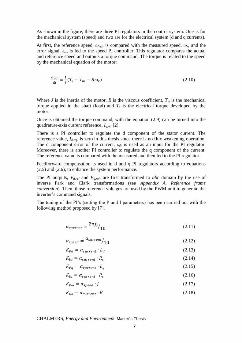
Simulink. Figure 2.4 shows the motor model used.
Page 22
10 CHALMERS, Energy and Environment, Master’s Thesis
Figure 2.4: Simulink model of the PMSM.
Controller model
In Figure 2.5 the whole controller system is presented. The proportional, integral and
anti windup parts as well as a saturation blocks for the torque limit are shown in the
figure.
Page 23
CHALMERS, Energy and Environment, Master´s Thesis
11
Figure 2.5: Control diagram for FOC of PMSM.
Page 24
12 CHALMERS, Energy and Environment, Master’s Thesis
Table 2.1: Control parameters
Parameter Unit Value Description
fs Hz 5.000 Switching frequency
Vdc V 400 DC bus voltage
Kpc_d -- Proportional constant of d-axis current regulator
Kic_d -- Integral constant of d-axis current regulator
Kpc_q -- Proportional constant of q-axis current regulator
Kic_q -- Integral constant of q-axis current regulator
Kpw -- Proportional constant of speed regulator
Kiw -- Integral constant of speed regulator
Id_ref A 0 d-axis current command
1st step.value rad/s 34,906 Speed reference for the first step
1st step.time s 0 Time when first step happens
2nd
step.value rad/s 17,453 Speed reference for the second step
2nd
step.time s 3 Time when the second step happens
*Variable step, max step size of 5e-5 s, solver ode45
Table 2.2: Motor parameters.
Parameter Unit Value Description
Rs Ω 7,1 Stator resistance
Ld H 30e-3 Direct-axis inductance
Lq H 30e-3 Quadrature-axis inductance
p -- 3 Pole pairs
phi_pm Vs 0,12 Permanent magnet flux
B Ns/m 0,002 Viscous coefficient
J kgm2 5,8e-4 Inertia
Page 25
CHALMERS, Energy and Environment, Master´s Thesis
13
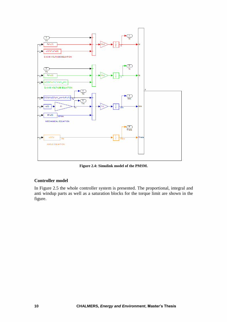
Simulation Results
Now, the results of the simulation are presented.
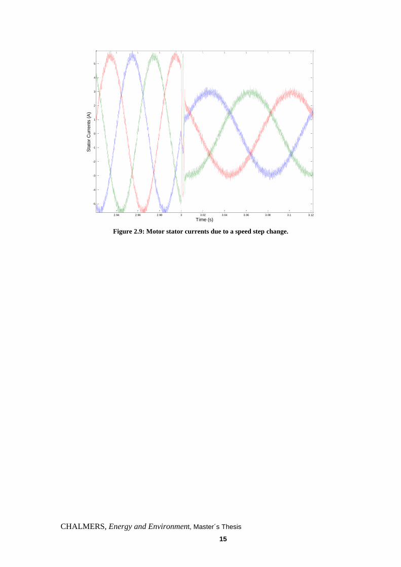
Figure 2.6 shows the speed response of the system due to a step change in the
command. The electrical torque and the stator currents are shown in Figure 2.7,
Figure 2.8 and Figure 2.9 respectively.
As it is shown in these figures, the system has a good dynamic response.
Figure 2.6: Mechanical speed (command in blue, actual in green).
0 1 2 3 4 5 60
5
10
15
20
25
30
35
Time (s)
Mechanic
al S
peed (
rad/s
)
Page 26
14 CHALMERS, Energy and Environment, Master’s Thesis
Figure 2.7: Electrical torque.
Figure 2.8: Motor stator current in abc domain.
0 1 2 3 4 5 6-4
-3
-2
-1
0
1
2
3
4
Time (s)
Torq
ue (
Nm
)
0 1 2 3 4 5 6-6
-4
-2
0
2
4
6
Time (s)
Sta
tor
Curr
ents
(A
)
Page 27
CHALMERS, Energy and Environment, Master´s Thesis
15
Figure 2.9: Motor stator currents due to a speed step change.
2.94 2.96 2.98 3 3.02 3.04 3.06 3.08 3.1 3.12
-5
-4
-3
-2
-1
0
1
2
3
4
5
Time (s)
Sta
tor
Curr
ents
(A
)
Page 28
16 CHALMERS, Energy and Environment, Master’s Thesis
3 Practical implementation of a PMSM drive system
An experimental system is designed to implement FOC of IPM that is explained in
this chapter. System architecture is presented firstly. Afterwards, the hardware
components are presented. Practical measurements results are added also.
3.1 General hardware overview
Figure 3.1 shows a simple schematic diagram of the system. The equipments used in
the lab setup of this thesis are listed below:
Permanent magnet synchronous machine
Inverter
Voltage, current, rotor angle and speed measurement equipments
dSpace DS1103 control system
24V relay
An optocard for over current protection
Various electrical items such as wires, connectors, grounding and so on
All these equipment are installed/organized in the following way:
A measurement box that includes:
- DC voltage source that provides the equipments with
- Three voltage transducers UMAT2 with three channels for voltage
measurements each one
- Seven current sensors LEM LA 50-S for current measurements
- A resolver-to-digital converter that measures rotor angle and speed
- Connector terminals to electrically link different components
The inverter box which includes:
- A voltage source that supplies the inverter control system
- A voltage source that feeds the grid contactor
- A four leg switch-mode inverter that uses Mosfet switches (one leg is
spare)
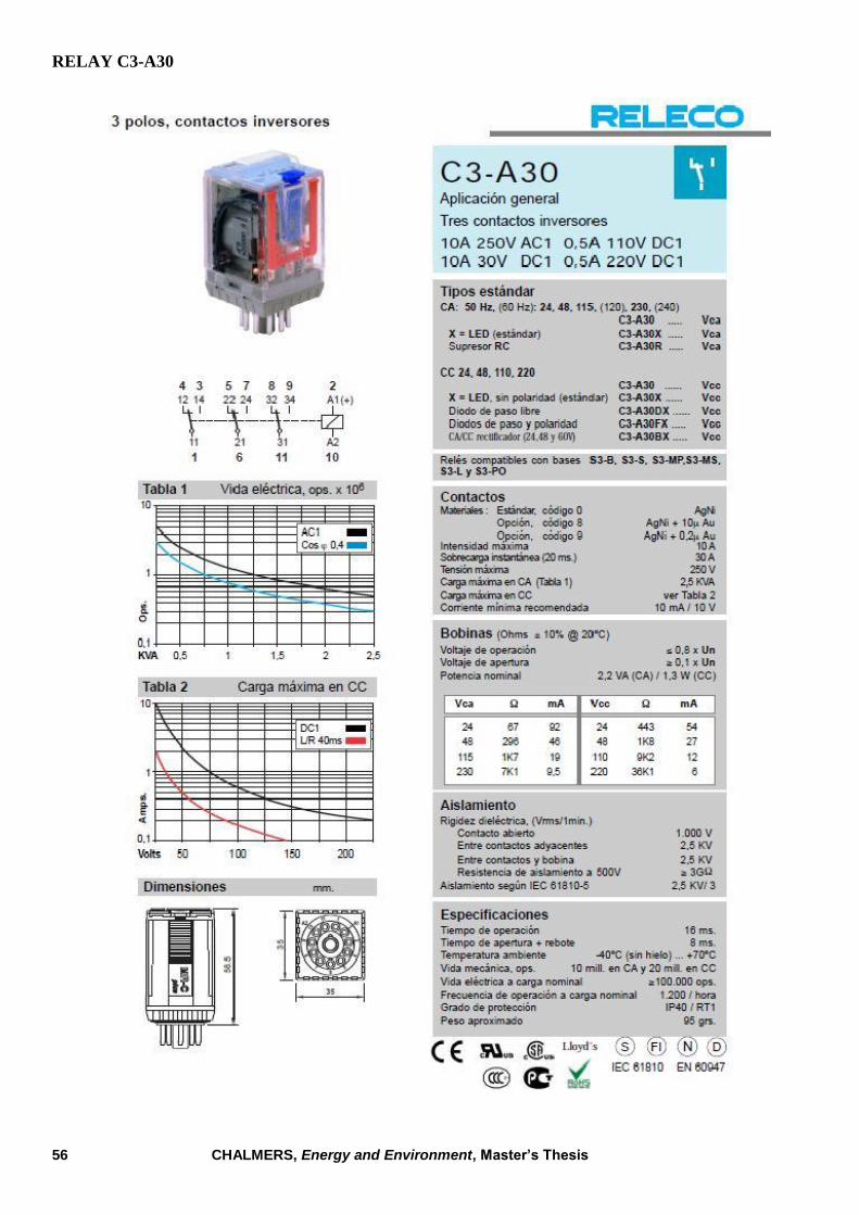
- A relay (C3-A 30) for the PMSM secondary winding connection to the
grid
- A designed electronic board to drive the relay
The PMSM with double stator windings and the resolver already installed on
the shaft. Resolver coils are available from the motor through a 12-pin
connector installed in the motor housing.
Control system is based on the dSpace, including the following parts:
- Two CP1103 dSpace board with analog and digital I/O
- A CLP1103 dSpace board with luminous LEDs that show the state of
the different signals
Page 29
CHALMERS, Energy and Environment, Master´s Thesis
17
- The optocard, that in case of over current in inverter, shuts down the
PWM signal to the transistors of the inverter to avoid damaging the
converter
- A DIO interface card that receives the measurement signals and send
an error signal to the optocard in case of over currents
To check all the connections inside each subsystem and between them, see Appendix
C. Lab setup diagrams.
As mentioned before, the control system will be expanded to serve as an integrated
charger described in [9]. So the secondary winding voltages and currents are
measured by the transducers. Moreover, there is a relay for connecting the three-phase
grid voltages to the secondary set of windings.
Page 30
18 CHALMERS, Energy and Environment, Master’s Thesis
Figure 3.1: Simple schematic diagram of the drive system.
Page 31
CHALMERS, Energy and Environment, Master´s Thesis
19
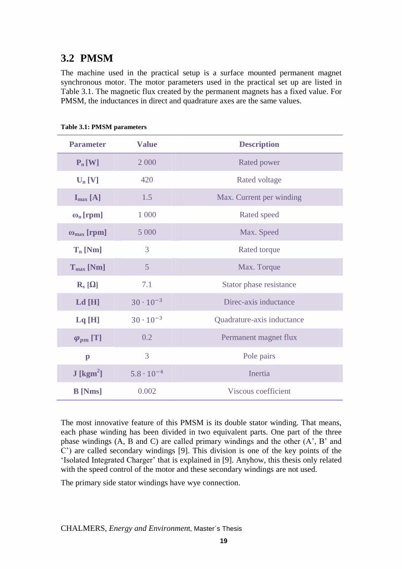
3.2 PMSM
The machine used in the practical setup is a surface mounted permanent magnet
synchronous motor. The motor parameters used in the practical set up are listed in
Table 3.1. The magnetic flux created by the permanent magnets has a fixed value. For
PMSM, the inductances in direct and quadrature axes are the same values.
Table 3.1: PMSM parameters
Parameter Value Description
Pn [W] 2 000 Rated power
Un [V] 420 Rated voltage
Imax [A] 1.5 Max. Current per winding
ωn [rpm] 1 000 Rated speed
ωmax [rpm] 5 000 Max. Speed
Tn [Nm] 3 Rated torque
Tmax [Nm] 5 Max. Torque
Rs [Ω] 7.1 Stator phase resistance
Ld [H] Direc-axis inductance
Lq [H] Quadrature-axis inductance
[T] 0.2 Permanent magnet flux
p 3 Pole pairs
J [kgm2] Inertia
B [Nms] 0.002 Viscous coefficient
The most innovative feature of this PMSM is its double stator winding. That means,
each phase winding has been divided in two equivalent parts. One part of the three
phase windings (A, B and C) are calledprimarywindingsandtheother(A‟,B‟and
C‟)are called secondary windings [9]. This division is one of the key points of the
„IsolatedIntegratedCharger‟that is explained in [9]. Anyhow, this thesis only related
with the speed control of the motor and these secondary windings are not used.
The primary side stator windings have wye connection.
Page 32
20 CHALMERS, Energy and Environment, Master’s Thesis
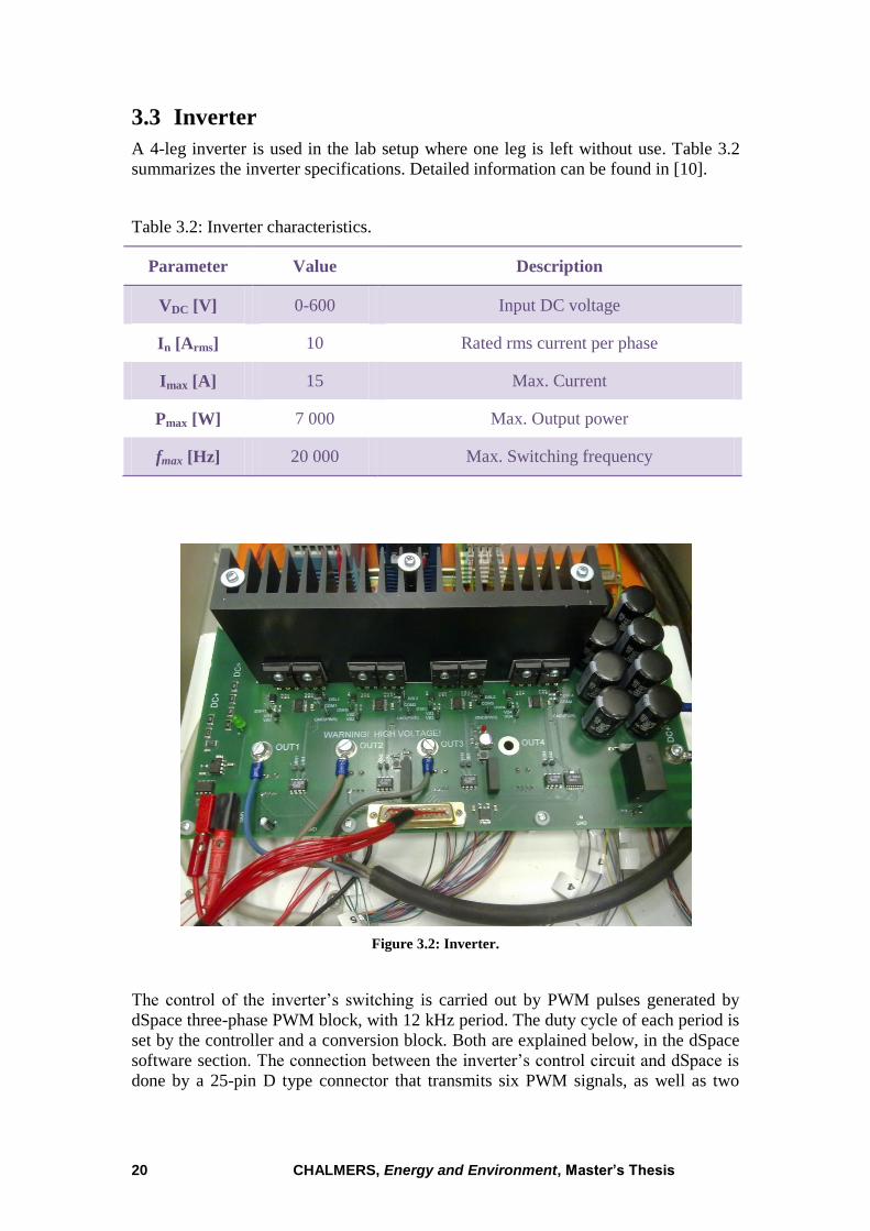
3.3 Inverter
A 4-leg inverter is used in the lab setup where one leg is left without use. Table 3.2
summarizes the inverter specifications. Detailed information can be found in [10].
Table 3.2: Inverter characteristics.
Parameter Value Description
VDC [V] 0-600 Input DC voltage
In [Arms] 10 Rated rms current per phase
Imax [A] 15 Max. Current
Pmax [W] 7 000 Max. Output power
fmax [Hz] 20 000 Max. Switching frequency
Figure 3.2: Inverter.
The control of the inverter‟s switching is carried out by PWM pulses generated by
dSpace three-phase PWM block, with 12 kHz period. The duty cycle of each period is
set by the controller and a conversion block. Both are explained below, in the dSpace
software section.Theconnectionbetweentheinverter‟scontrolcircuitanddSpaceis
done by a 25-pin D type connector that transmits six PWM signals, as well as two
Page 33
CHALMERS, Energy and Environment, Master´s Thesis
21
more command signals (relay and fault clear) needed for the inverter‟s start up
process.
To start up the inverter, the following steps should be taken:
Connect all necessary cables (+15V, DC supply, control system and load)
Turn on the control system
Turn on the low voltage supply
Turn on the high voltage supply
Start the control system by:
1. Turn on the relay when the DC voltage has reached the desired level (~1s)
2. Set FLT_CLR high
3. Start switching
4. Set FLT_CLR low
Once these steps are done, the inverter is ready for normal use [10].
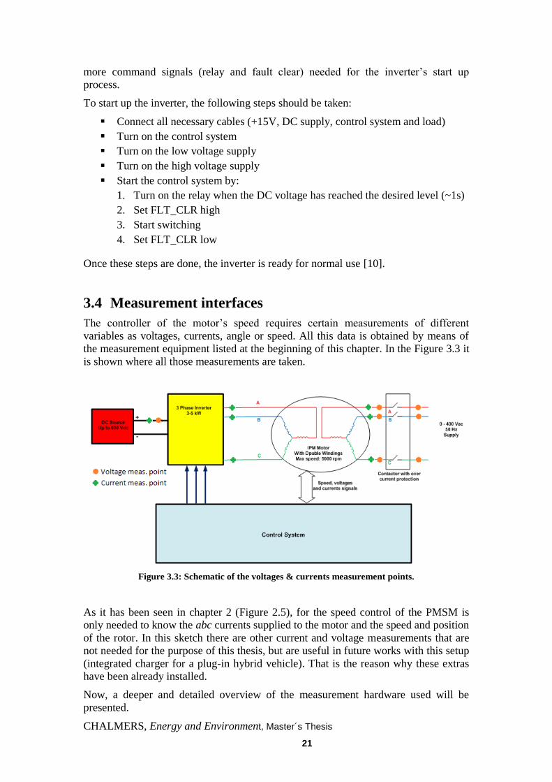
3.4 Measurement interfaces
The controller of the motor‟s speed requires certain measurements of different
variables as voltages, currents, angle or speed. All this data is obtained by means of
the measurement equipment listed at the beginning of this chapter. In the Figure 3.3 it
is shown where all those measurements are taken.
Figure 3.3: Schematic of the voltages & currents measurement points.
As it has been seen in chapter 2 (Figure 2.5), for the speed control of the PMSM is
only needed to know the abc currents supplied to the motor and the speed and position
of the rotor. In this sketch there are other current and voltage measurements that are
not needed for the purpose of this thesis, but are useful in future works with this setup
(integrated charger for a plug-in hybrid vehicle). That is the reason why these extras
have been already installed.
Now, a deeper and detailed overview of the measurement hardware used will be
presented.
Page 34
22 CHALMERS, Energy and Environment, Master’s Thesis
3.4.1 Voltage measurements
For the voltage measurements, three voltage transducers UMAT2 have been used.
Each transducer has three different channels, as can be seen in Figure 3.4, with a
common neutral point for three phase voltage measures. As far as it is only needed 7
channels, two of the transducers are used for two different three phase voltage
measurements and the third transducer has only one channel in use, for measuring the
DC voltage input of the inverter.
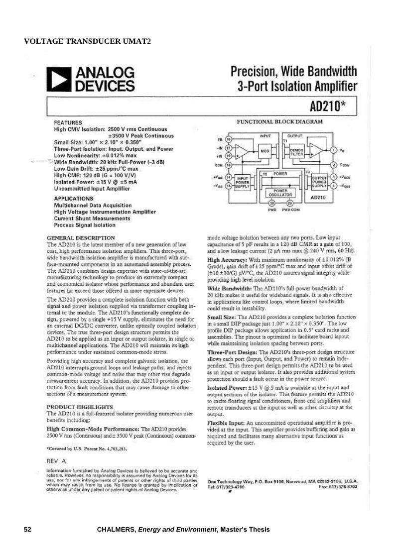
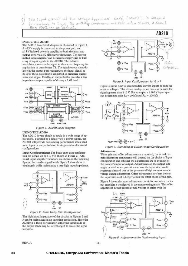
The transducer cards work as follows: first, the input voltage goes through a resistor
ladder that reduces the voltage level. After, the reduced signal goes to the AD210
electronic device, an isolated amplifier.
Figure 3.4: Voltage transducer UMAT2.
Resistors ladder design
The resistor ladder had to be designed and soldered before the testing and mounting of
the transducer. Figure 3.5 shows the used resistors ladder network. For this purpose
and considering that the voltage range to be measured is and the output
signals of the transducers should be in the range , the following procedure has
been performed:
Figure 3.5: Sketch of the resistor ladder of the UMAT2 transducer.
Page 35
CHALMERS, Energy and Environment, Master´s Thesis
23
where the initial conditions are:
(3.1).
And the relation between both voltages corresponds to a voltage divider:
(3.2).
According to (3.2), the resistors values chosen are:
This gives the proportion between input and output voltage:
(3.3).
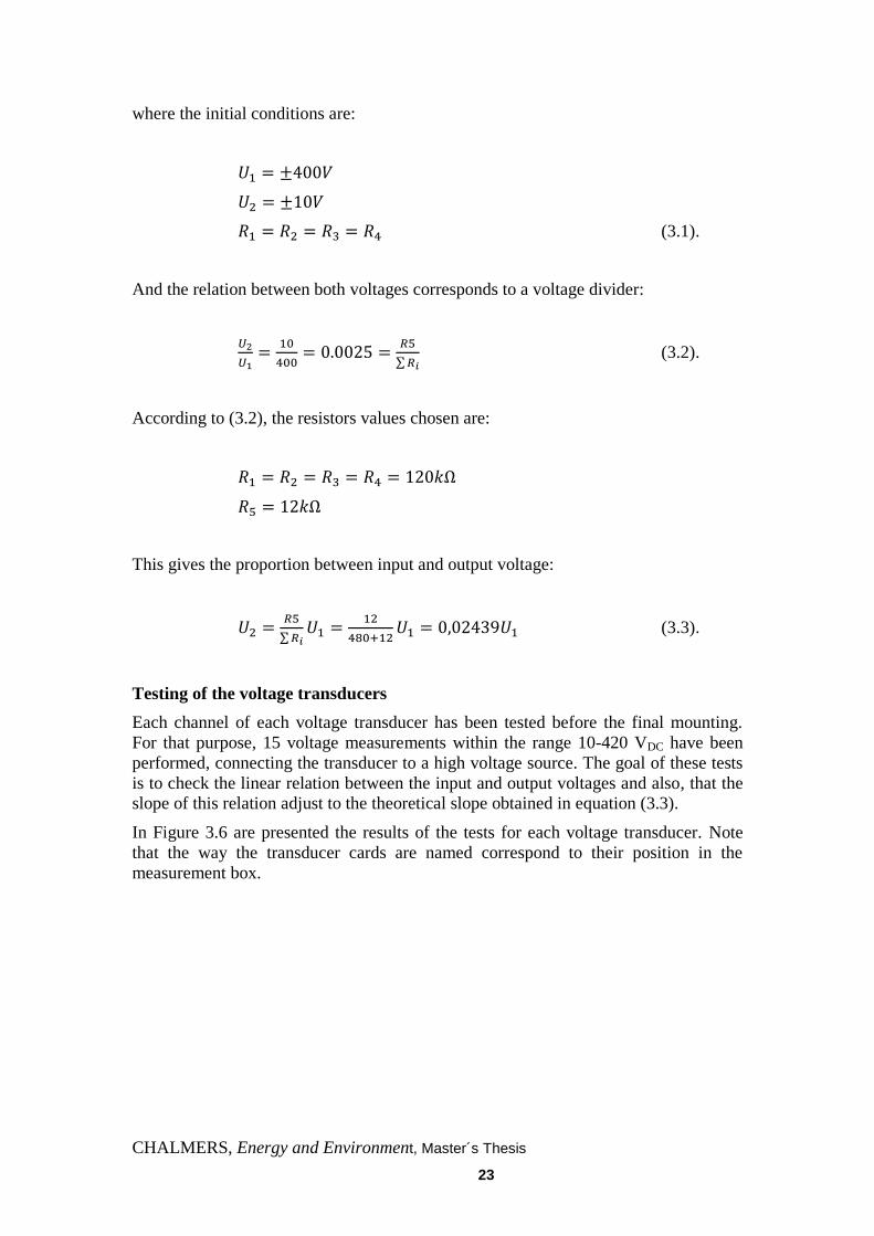
Testing of the voltage transducers
Each channel of each voltage transducer has been tested before the final mounting.
For that purpose, 15 voltage measurements within the range 10-420 VDC have been
performed, connecting the transducer to a high voltage source. The goal of these tests
is to check the linear relation between the input and output voltages and also, that the
slope of this relation adjust to the theoretical slope obtained in equation (3.3).
In Figure 3.6 are presented the results of the tests for each voltage transducer. Note
that the way the transducer cards are named correspond to their position in the
measurement box.
Page 36
24 CHALMERS, Energy and Environment, Master’s Thesis
Figure 3.6: Voltage transducers test.
The voltage transducers have a good performance in terms of linearity and error. Now,
the real slope of each channel is computed, in order to use that value in the future
programming for the real time application that will control the lab tests. The errors
computed correspond to a nominal voltage measure (400 V).
For the upper transducer the slopes of each channel are:
Channel 1, slope = 0,02411. Error = 1,189%.
Channel 2, slope = 0,02411. Error = 1,291%.
Channel 3, slope = 0,02408. Error = 1,189%.
For the mid transducer the slopes of each channel are:
Channel 1, slope = 0,02485. Error = 1,681%.
Channel 2, slope = 0,02488. Error = 1,886%.
Channel 3, slope = 0,02459. Error = 0,877%.
For the lower transducer the slope is:
0 2 4 6 8 10 120
50
100
150
200
250
300
350
400
450
U1 [V]
U2 [
V]
black = theor. red = chan.3
0 2 4 6 8 10 120
50
100
150
200
250
300
350
400
450
U1 [V]
U2 [
V]
black = theor. blue = chan.1 green = chan.2 red = chan.3
0 2 4 6 8 10 120
50
100
150
200
250
300
350
400
450
U1 [V]
U2 [
V]
black = theor. blue = chan.1 green = chan.2 red = chan.3
Page 37
CHALMERS, Energy and Environment, Master´s Thesis
25
Channel 3, slope = 0,02426. Error = 0,499%.
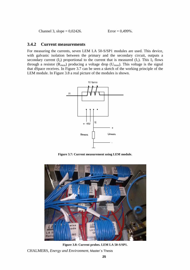
3.4.2 Current measurements
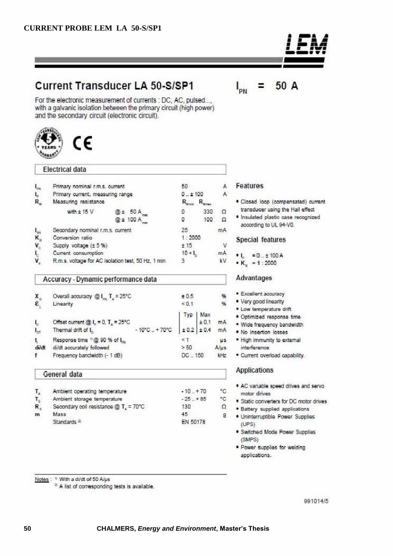
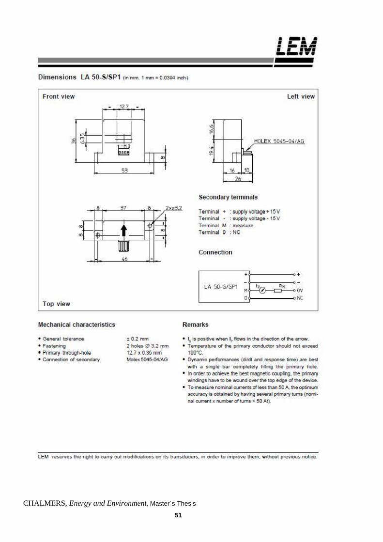
For measuring the currents, seven LEM LA 50-S/SP1 modules are used. This device,
with galvanic isolation between the primary and the secondary circuit, outputs a
secondary current (I2) proportional to the current that is measured (I1). This I2 flows
through a resistor (Rmeas) producing a voltage drop (Umeas). This voltage is the signal
that dSpace receives. In Figure 3.7 can be seen a sketch of the working principle of the
LEM module. In Figure 3.8 a real picture of the modules is shown.
Figure 3.7: Current measurement using LEM module.
Figure 3.8: Current probes. LEM LA 50-S/SP1.
Page 38
26 CHALMERS, Energy and Environment, Master’s Thesis
Parameters design
The voltage signal Umeas should be between . It is needed to choose an appropriate
number of turns of the primary circuit as well as a value for Rmeas (between 0-300Ω,
according to the data sheet), so the relation between the output voltage and the input
current is determined. To begin with, the relation between the input and output currents,
according to the data sheet of the LEM module is:
(3.4)
Where N is the number of turns. For nominal currents below 50 A, a better accuracy is
obtained by having several primary turns. So N = 10 turns is selected. Now, the relation
between the secondary current and the output voltage has to be used to compute Rmeas:
(3.5)
Combining equations (3.4) and (3.5) it is obtained:
(3.6)
If we choose a Rmeas =200Ω,thelinearrelationbetweenI1 and Umeas is unitary.
Testing of the current modules
Each current module has been tested with 26 different current values between 0-6 A.
The results of these tests showed that a good linear relation exists between the input
current and the output voltage and that the experimental slope of this relation is almost
the expected value (less than 1% error in the worst case). Anyway, the experimental
slopes, shown in Table 3.3, are the value used in the lab tests.
Table 3.3: Experimental slopes of the LEM modules.
LEM module 1 2 3 4 5 6 7
Experimental
slope [V/A] 1,0040 0,9966 0,9773 1,0060 0,9833 1,0026 0,9906
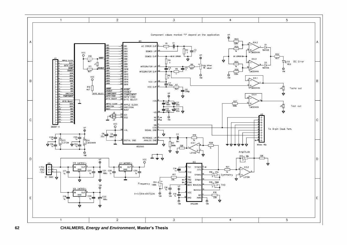
3.4.3 Position and speed measurements
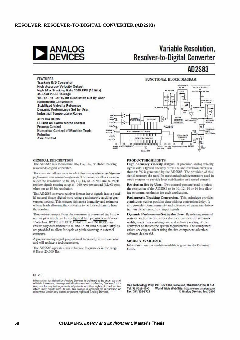
Both, rotor position and speed are measured with a resolver-to-digital converter. This
converter, pictured in Figure 3.9: Resolver-to-digital PBC., generates and sends a
Page 39
CHALMERS, Energy and Environment, Master´s Thesis
27
sinusoidal reference waveform to a coil mounted in the rotor, and measure induced
voltages in the two coils mounted on the stator. These two measured signals are
processed by the resolver-to-digital converter, which is AD2S83 in this case, and the
angle is extracted in a digital word. The number of digital bits for the angle
measurement is programmable by the device.
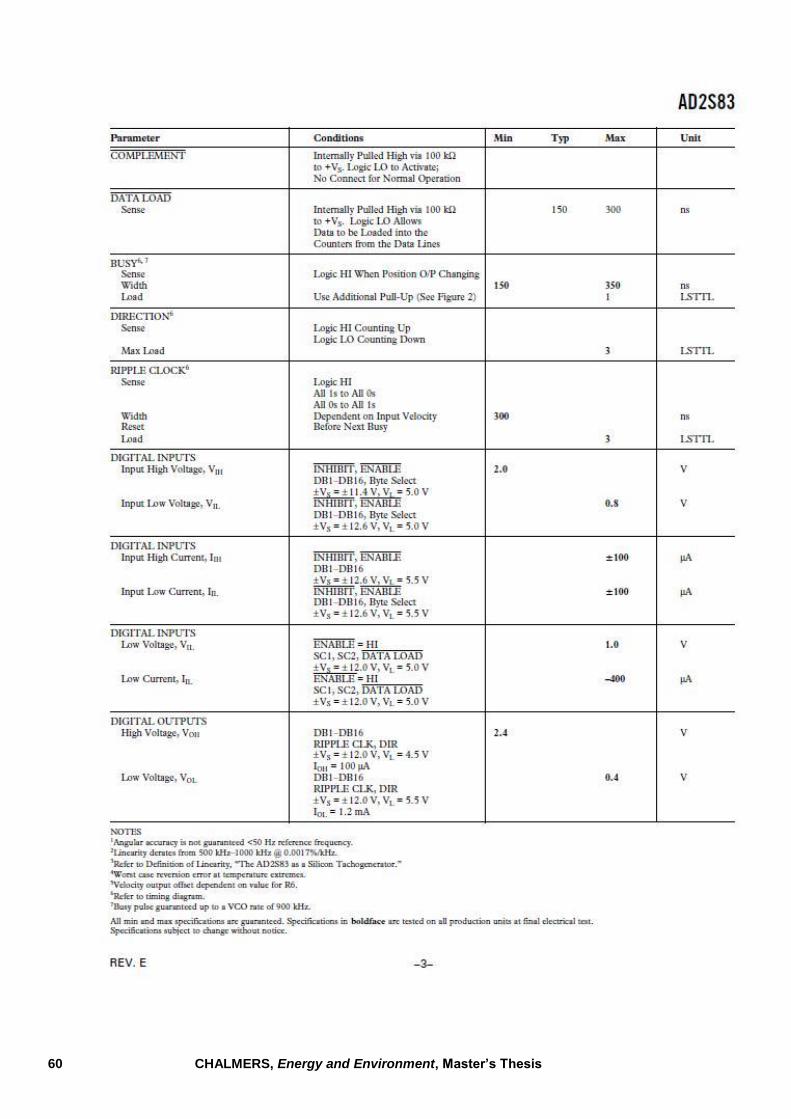
In the board of the converter there is an option for choosing the resolution. In our case
the appropriate resolution is 12 bit, which is the highest one that permits measuring up
to 5000 rpm. Some other trimming had to be done to tune the reference wave generation
or remove the offset in the output. Finally, some external components have to be
mounted in the printed circuit board. The selection is shown in Table 3.4.
Figure 3.9: Resolver-to-digital PBC.
Table 3.4: External component selection for the resolver-to-digital PBC.
Components selection Value
Components Typ. Values Comments For 12-bit Unit
s
HF Filter
R1 15 - 6 k May be omitted. Then, R2=R3 2,400E+04 Ω
R2 15 - 6 k Same value than R1 2,400E+04 Ω
C1 / πR1fref) Same value than C2 6,631E-10 F
C2 1/(2πR1fref) May be omitted. Then, C1=C3 6,631E-10 F
Gain scaling
R4* Edc/(300e-9) If R1 & C2 are used 1,333E+05 Ω
Edc/(100e-9) If R1 & C2 aren't used 4,000E+05 Ω
AC coup
of ref. input
R3 k
1,000E+05 Ω
C3 > 1/(R3fref) R3 in ohms 1,000E-09 F
Max R6** T = VCOrate/(2N) N=resolution, VCOrate=trackin 83,333 rps
Page 40
28 CHALMERS, Energy and Environment, Master’s Thesis
track rate
rate(rps)
R6=6,81e10/(Tn)
n=bits per revolution, min R6 6 k
1,995E+05 Ω
Close-loop BW
select
C4 21/(R6fbw2) Choose fbw according to
resolution 1,684E-11 F
C5 5C4
8,421E-11 F
R5 4/(2πfbwC5)
3,024E+06 Ω
Where:
* for 12 bit resolution
** bits per revolution
Note: according to the data sheet, should be 4 times lower than for a 12 bit
resolution.
Withthesecomponent‟svalues, theoutputfromthespeedmeter is presented in Table
3.5.
Table 3.5: Output voltage for different rotor speeds.
Speed Current Vout
rpm Hz µA V
100 1,667 0,803 0,160
250 4,167 2,008 0,400
500 8,333 4,016 0,800
750 12,500 6,024 1,200
1000 16,667 8,031 1,600
1500 25,000 12,047 2,400
2000 33,333 16,063 3,200
2500 41,667 20,078 4,000
3000 50,000 24,094 4,800
3500 58,333 28,110 5,600
4000 66,667 32,125 6,400
4500 75,000 36,141 7,200
5000 83,333 40,157 8,000
Testing and tuning of the resolver-to-digital transducer
Page 41
CHALMERS, Energy and Environment, Master´s Thesis
29
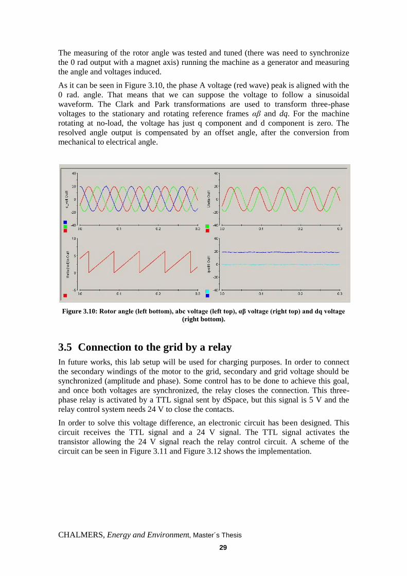
The measuring of the rotor angle was tested and tuned (there was need to synchronize
the 0 rad output with a magnet axis) running the machine as a generator and measuring
the angle and voltages induced.
As it can be seen in Figure 3.10, the phase A voltage (red wave) peak is aligned with the
0 rad. angle. That means that we can suppose the voltage to follow a sinusoidal
waveform. The Clark and Park transformations are used to transform three-phase
voltages to the stationary and rotating reference frames αβ and dq. For the machine
rotating at no-load, the voltage has just q component and d component is zero. The
resolved angle output is compensated by an offset angle, after the conversion from
mechanical to electrical angle.
Figure 3.10:Rotorangle(leftbottom),abcvoltage(lefttop),αβvoltage(righttop)anddqvoltage
(right bottom).
3.5 Connection to the grid by a relay
In future works, this lab setup will be used for charging purposes. In order to connect
the secondary windings of the motor to the grid, secondary and grid voltage should be
synchronized (amplitude and phase). Some control has to be done to achieve this goal,
and once both voltages are synchronized, the relay closes the connection. This three-
phase relay is activated by a TTL signal sent by dSpace, but this signal is 5 V and the
relay control system needs 24 V to close the contacts.
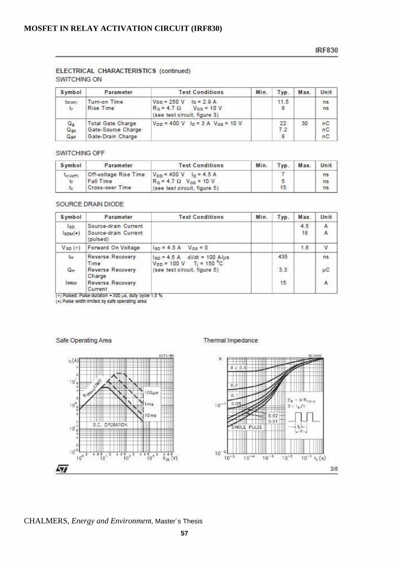
In order to solve this voltage difference, an electronic circuit has been designed. This
circuit receives the TTL signal and a 24 V signal. The TTL signal activates the
transistor allowing the 24 V signal reach the relay control circuit. A scheme of the
circuit can be seen in Figure 3.11 and Figure 3.12 shows the implementation.
Page 42
30 CHALMERS, Energy and Environment, Master’s Thesis
24 V
TTL
(5 V)
0 V
100 kΩ
1 kΩ 0,1 µF 15 V
Figure 3.11: Scheme of the relay activation circuit.
Figure 3.12: Three-phase relay (left) and relay activation circuit (right).
3.6 dSpace system
The dSpace system is a tool used to build real-time control systems. It is used to connect
different kind of signals (analogue or digital) that measurement devices obtain to a
computer, as well as send signals from the computer to the devices in order to control
them.
The dSpace system is the interface between the physical world (motor, inverter,
measure sensors...) and the computer, from where the lab tests is controlled and the
results are plotted. The dSpace system model used in this setup is CP1103 system, with
different analogue I/O and digital I/O.
The controller has to be programmed and then, by means of the analogue and digital
I/O, some command signals are sent to the system and the measured values are received.
Page 43
CHALMERS, Energy and Environment, Master´s Thesis
31
Software part
The dSpace programming has been carried out using Simulink. Most of the model is
equal to the one used in chapter 2 for the simulations. Only few parts have been
changed, added or removed. These modifications are shown in Appendix E. dSPace
software implementation.
Special attention should be placed in the Simulation > Configuration Parameters. The
next modifications should be done before running a real time application:
The stop time is setto“inf”.
Thesolvertypeshouldbe“Fixed-step”.
The solver is“ode1 (Euler)”.
The block reduction option in the optimization menu should be unmarked.
Without these modifications, the program would return an error message when trying to
compile.
The modifications carried out to the original Simulink program (the one used for the
simulations in chapter 2) are as following:
Some ADC block are added for receiving the voltage, current and speed
measurements. Apart from the linear conversion mentioned in the measurement
equipment description, a gain of 190 has to be added because dSpace reduces in
10 times the input value (a input correspond to in Simulink).
Theinverter‟smodelis removed. Instead there is the real inverter. Some blocks
are added to initialize the inverter.
The motor model is removed. Instead there is the real PMSM.
The PWM block is changed for the PWM three-phase generation that includes
the RTI library in Simulink. Now the voltage command get to a conversion
block, where it is obtained the duty cycle of each phase of thee PWM, and these
signal are the input to the PWM block.
A new block dedicated to the resolver has to be added. The resolver is driven by
the inhibit signal. This is a square signal that indicates when the data in the
resolver transducer has to be updated and when has to be sent to dSpace. When
inhibit is low data is sent and when is high, data is being updated. This inhibit
signal (12 kHz square) is also used to trigger the interrupt that drives the
controller block.
The controller, as well as the Clark and Park transformations remains the same.
The system has been organized in two main blocks: measurements and controller. The
measurement block is triggered with the PWM interrupt block. The purpose of that is to
synchronize all the measurements with the peak of the carrier wave (triangular wave) of
the PWM. All the measurements are captured at the same time (with a sampling time of
12 kHz). Then, the controller block is triggered with an interrupt generated within the
measurement block, so when the data capture is finished all the operations required for
the control will begin.
All the changes performed to the original Simulink blocks of chapter 2 can be seen in
Appendix E. dSpace software implementation.
Page 44
32 CHALMERS, Energy and Environment, Master’s Thesis
The other software tool used is ControlDesk. With ControlDesk is possible to create
instrument panels whit control, display and plotting possibilities. By connecting the
Simulink variables to plotters, slide bars, displays, leds...etc the user can modify
constants or command values, or check the current, speed or torque waveforms. Figure
3.13 shows the instrumentation panel used for this experiment.
Figure 3.13: Layout of the dSpace instrumentation panel.
Hardware part
The dSpace boards CP1103 and CPL1103, shown in Figure 3.14, are connected to the
host PC. Then, these boards provide some inputs and outputs to be connected to the
external devices. In this project 6 analogue inputs (ADC) are being used, as well as the
master and slave digital I/O. The connections are the following (and can be seen also in
Appendix C. Lab setup diagrams):
One analogue input for the speed
Two analogue inputs for the DC current and voltage (input of the inverter)
Three analogue inputs for the three phase currents which feed the PMSM
The master digital I/O for controlling the resolver-to-digital board, and read the
12-angle bits
TheslavedigitalI/OforthePWMpulses,theinverter‟sinitializationcommands
and the grid contactor operation
Page 45
CHALMERS, Energy and Environment, Master´s Thesis
33
The hardware system is already prepared to use another 9 analogue inputs that measure
the three phase secondary currents and voltages as well as the grid voltage, when the
charging tests are performed.
Figure 3.14: dSpace connections boards CP1103 and CPL1103.
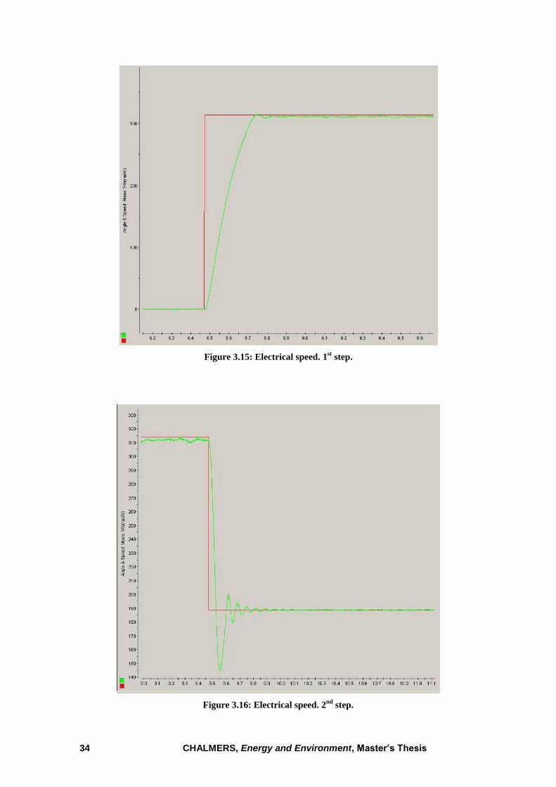
3.7 Experimental results
Now, the results of the experimental test are presented.
Figure 3.15 and Figure 3.16 shows the speed response of the system due to a step
change in the speed command. The zoomed stator currents for each speed step are
shown in Figure 3.17 and Figure 3.18, respectively.
As it is shown in these figures, the system has a good dynamic response.
Page 46
34 CHALMERS, Energy and Environment, Master’s Thesis
Figure 3.15: Electrical speed. 1st step.
Figure 3.16: Electrical speed. 2nd
step.
Page 47
CHALMERS, Energy and Environment, Master´s Thesis
35
Figure 3.17: Stator currents in abc domain due to the first speed step.
Figure 3.18: Stator currents in abc domain due to the second speed step.
Page 48
36 CHALMERS, Energy and Environment, Master’s Thesis
4 Conclusions and future work
4.1 Conclusions
Field-oriented control of a permanent magnet synchronous motor is designed, simulated
and implemented in this thesis.
Firstly, the whole drive system is simulated by the use of Matlab/Simulink. With the
motor equations, a model for the machine has been developed in Simulink, as well as
models for the PWM signal generator, inverter, controller and Clark and Park
transformations. The results of the simulation show the good response of the model
when tracking a command speed.
Afterwards a lab setup was implemented using a 2 kW PMSM and dSpace as the
computer-system interface. After the calibration of every measuring device and the
proper corrections of the controller model, some lab tests were carried up to check the
validity of the simulation results. The results show that the system has a good dynamic
response.
4.2 Future work
The current hardware will be extended to implement an isolated integrated charger as
explained in [9].
The classical PWM method is used to generate the requested motor voltages. To
improve the system performance in terms of torque ripple, power quality and better DC
voltage utilization, space vector modulation can be employed.
The speed is estimated by the measurement of the position. The speed estimation can be
improved by the use of Kalman filters.
Page 49
CHALMERS, Energy and Environment, Master´s Thesis
37
References
[1] Merzoug and Benalla, “Nonlinear Backstepping Control of Permanent Magnet
Synchronous Motor (PMSM)”, Department of Electrical Engineering, University of
Mentouri Constantine. Algier 2010.
[2] SongChi,“Position-sensorless control of permanent magnet synchronous machines
overwidespeedrange”.Thesis for the degree of Doctor, Department of Electrical and
Computer Engineering, Ohio State University.
[3] VictorR.Stefanovic,“Trends inACDriveApplications,”[4] Russel J. Kerkman,
GaryL.SkibinskiandDavidW.Schlegel,”ACDrives:Year2000(Y2K)andBeyond”,
Rockwell Automation, Standard Drives Division, 1999.
[5] F. Heydari, A. Sheikholeslami, K. G. Firouzjah amd S. Lesan. “Predictive Field-
Oriented Control of PMSM with SpaceVectorModulationTechnique”.Front.Electr.
Electron. Eng. China, 2010.
[6] Jorge Zambada, Microchip Corporation, “Sensorless Field Oriented Control of
PMSMMotors”.MicrochipTechnologyInc.,2007.
[7]LennartHarnefors,“ControlofVariable-Speed Drives”,Appliedsignalprocessing
and control, department of electronics, Mälardalen University, September 2002.
[8] Sylvain Lechat Sanjuan, “Voltage Oriented Control of Three-Phase Boost PWM
Converters”, Master of Science Thesis in Electric Power Engineering, Chalmers
University of Technology, Göteborg, 2010.
[9] Saeid Haghbin, “An Isolated Integrated Charger for Electric or Plug-in Hybrid
Vehicles” thesis for the degree of licentiate of engineering. Chalmers University of
Technology, department of Energy and Environment, division of Electric Power
Engineering. Göteborg, Sweden, 2011.
[10] Kristoffer Berntsson, “Four Phase Switch-Mode Inverter, Construction and
Evaluation”, Master of Science Thesis in Chalmers University of Thechnology,
department of Energy and Environment, division of Electric Power Engineering.
Göteborg, Sweden, 2010.
[11]C.C.Chan,“TheStateoftheArtofElectricandHybridVehicles”,Proceedingsof
the IEEE, Vol. 90, No. 2, February 2002.
[12] Saeid Haghbin, Sonja Lundmark, Ola Carlson andMatsAlaküla, “ACombined
Motor/Drive/Battery Charger Based on a Split-WindingsPMSM”,Chalmers University
of Technology, department of Energy and Environment, division of Electric Power
Engineering. Göteborg, Sweden, 2011
[13] Pragasen Pillay and Ramu Krishnan, “Application Characteristics of Permanent
MagnetSynchronousandBrushlessdcMotorsforServoDrives”,IEEETransactionsof
Industry Applications, Vol. 27, No. 5, September/October 1991.
[14]M.S.MerzougandF.Naceri,“ComparisonofField-Oriented Control and Direct
TorqueControlforPermanentMagnetSynchronousMotor(PMSM)”,WorldAcademy
of Science, Engineering and Technology 45, 2008.
Page 50
38 CHALMERS, Energy and Environment, Master’s Thesis
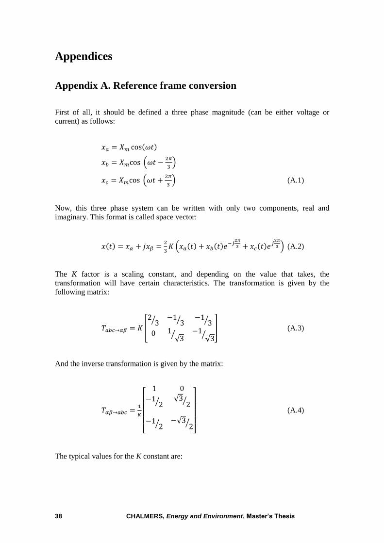
Appendices
Appendix A. Reference frame conversion
First of all, it should be defined a three phase magnitude (can be either voltage or
current) as follows:
(A.1)
Now, this three phase system can be written with only two components, real and
imaginary. This format is called space vector:
(A.2)
The K factor is a scaling constant, and depending on the value that takes, the
transformation will have certain characteristics. The transformation is given by the
following matrix:
(A.3)
And the inverse transformation is given by the matrix:
(A.4)
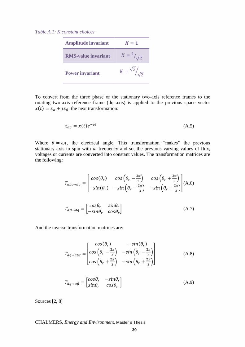
The typical values for the K constant are:
Page 51
CHALMERS, Energy and Environment, Master´s Thesis
39
Table A.1: K constant choices
Amplitude invariant
RMS-value invariant
Power invariant
To convert from the three phase or the stationary two-axis reference frames to the
rotating two-axis reference frame (dq axis) is applied to the previous space vector
the next transformation:
(A.5)
Where , the electrical angle. This transformation “makes” the previousstationary axis to spin with frequency and so, the previous varying values of flux,
voltages or currents are converted into constant values. The transformation matrices are
the following:
(A.6)
(A.7)
And the inverse transformation matrices are:
(A.8)
(A.9)
Sources [2, 8]
Page 52
40 CHALMERS, Energy and Environment, Master’s Thesis
Appendix B. Matlab code and Simulink block diagrams
Matlab code of the file Parameters.m
%////////////////////////////////////////////////////////////////////
% 2 kW motor parameters
%
% Master thesis student David Vindel Muñoz.
% Electric Power Engineering Department
% Chalmers Tekniska Högskola
%
% March 2011
%////////////////////////////////////////////////////////////////////
clear all
% PMSM parameters
Rs = 7.1; %Stator resistance Ld = 30e-3; %d-axis inductance Lq = 30e-3; %q-axis inductance phi_pm = 0.12; %Permanent magnet flux
p = 3; %Pole pairs J = 5.8e-4; %Inertia B = 0.002; %Viscous coefficient Wbase = 1000*pi/30; %Base speed Wmax = 5000*pi/30; %Max. speed Prated = 2000; %Rated power Trated = 3; %Rated torque
% Controller parameters
Vdc = 400;
% Current PI parameters
Fs = 10e3; %Inverter's Swithcing frequency 10[kHz]
alpha_i = 2*pi*Fs/10; %Parameter used for Kp & Ki
Kpc_d = alpha_i*Ld; %Prop.constant of d-axis current reg.
Kic_d = alpha_i*Rs; %Int. constant of d-axis current reg. Kpc_q = alpha_i*Lq; %Prop. constant of q-axis current reg. Kic_q = alpha_i*Rs; %Int. constant of q-axis current reg. % Speed PI parameters
alpha_w = alpha_i/10; %Parameter used for Kp & Ki Kpw = alpha_w*J; %Prop. constant of speed reg. Kiw = alpha_w*B; %Int. constant of speed reg.
Page 53
CHALMERS, Energy and Environment, Master´s Thesis
41
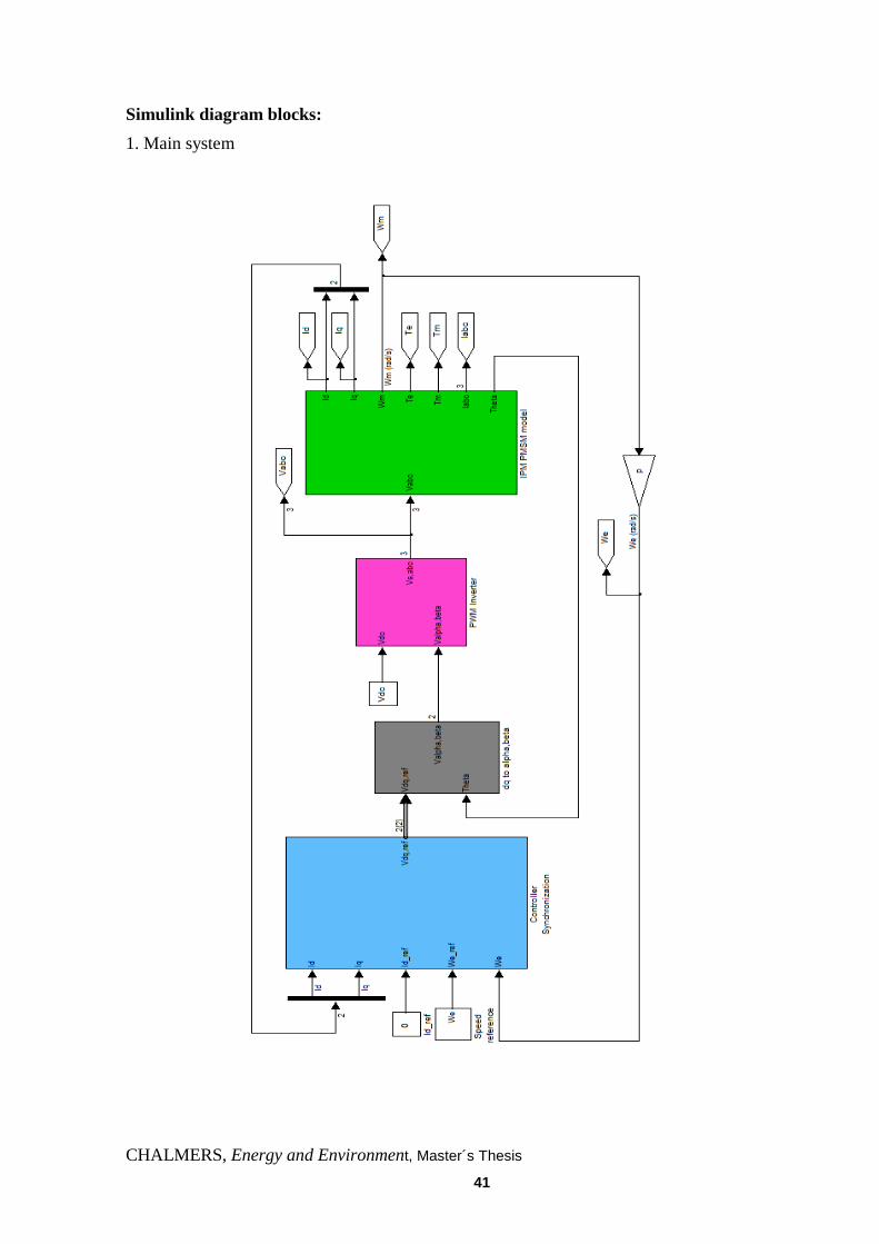
Simulink diagram blocks:
1. Main system
Page 54
42 CHALMERS, Energy and Environment, Master’s Thesis
2. Speed controller
Page 55
CHALMERS, Energy and Environment, Master´s Thesis
43
3. Clark & Park reference frame conversion (direct)
4. Clark & Park reference frame conversion (inverse)
5. PWM generation
Page 56
44 CHALMERS, Energy and Environment, Master’s Thesis
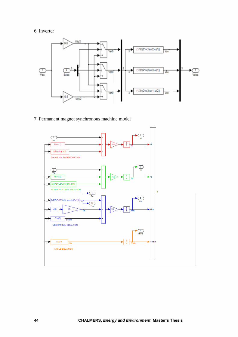
6. Inverter
7. Permanent magnet synchronous machine model
Page 57
CHALMERS, Energy and Environment, Master´s Thesis
45
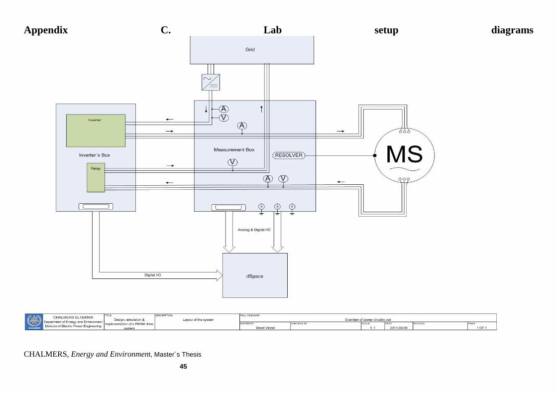
Appendix C. Lab setup diagrams
Page 58
46 CHALMERS, Energy and Environment, Master’s Thesis
Page 59
CHALMERS, Energy and Environment, Master´s Thesis
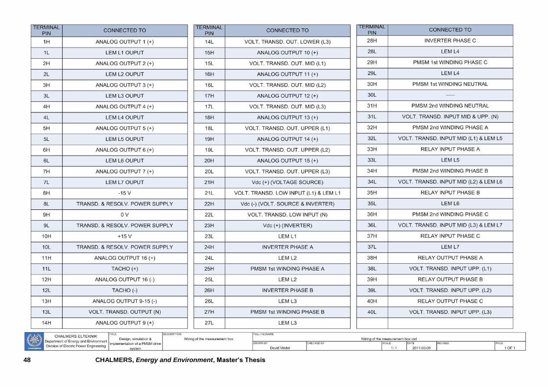
47
Page 60
48 CHALMERS, Energy and Environment, Master’s Thesis
Page 61
CHALMERS, Energy and Environment, Master´s Thesis
49
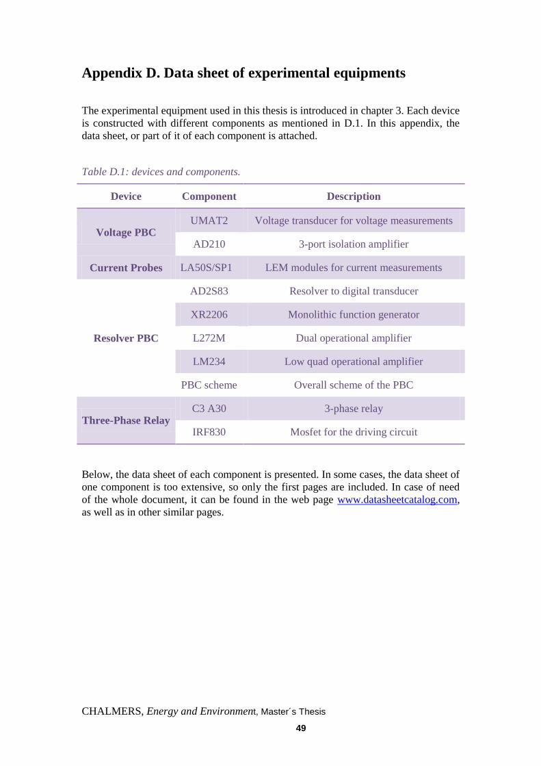
Appendix D. Data sheet of experimental equipments
The experimental equipment used in this thesis is introduced in chapter 3. Each device
is constructed with different components as mentioned in D.1. In this appendix, the
data sheet, or part of it of each component is attached.
Table D.1: devices and components.
Device Component Description
Voltage PBC UMAT2 Voltage transducer for voltage measurements
AD210 3-port isolation amplifier
Current Probes LA50S/SP1 LEM modules for current measurements
Resolver PBC
AD2S83 Resolver to digital transducer
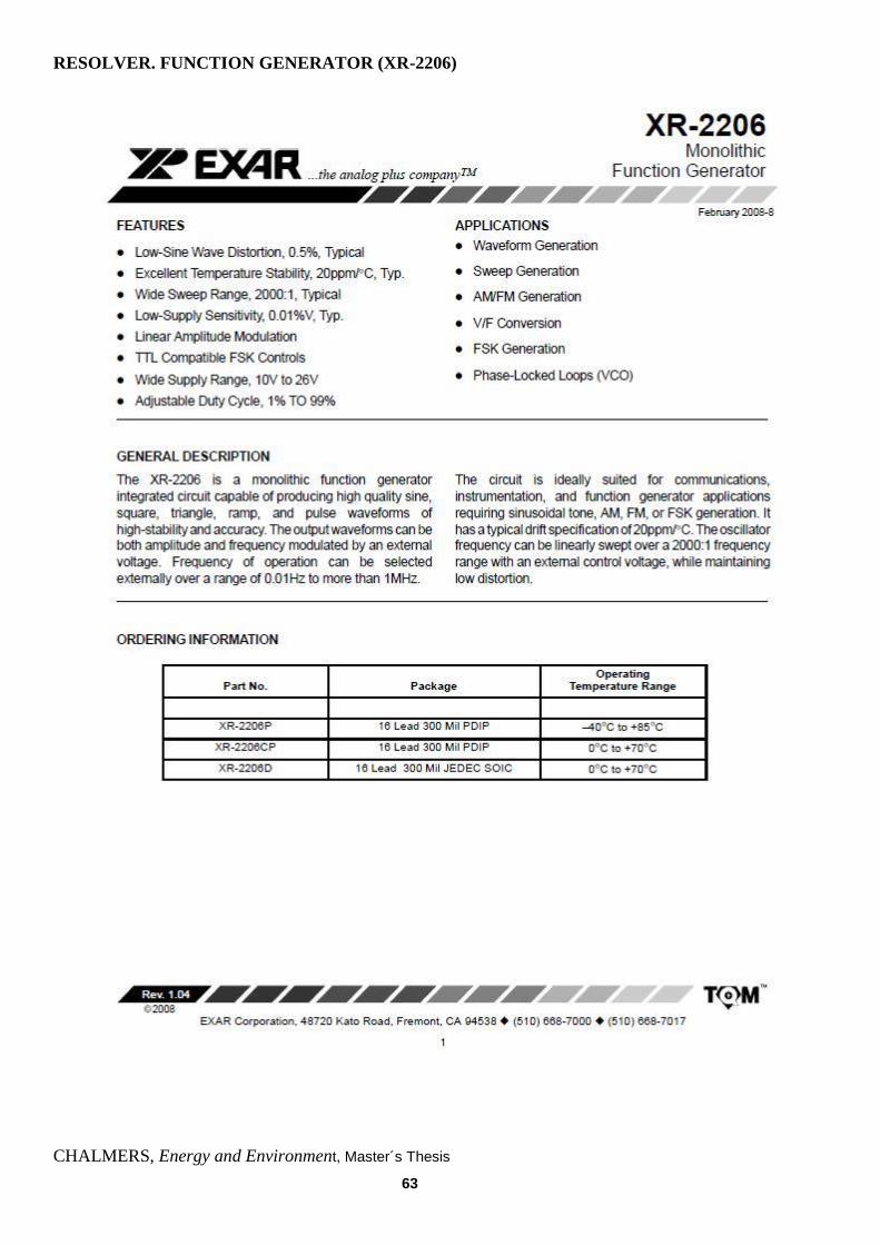
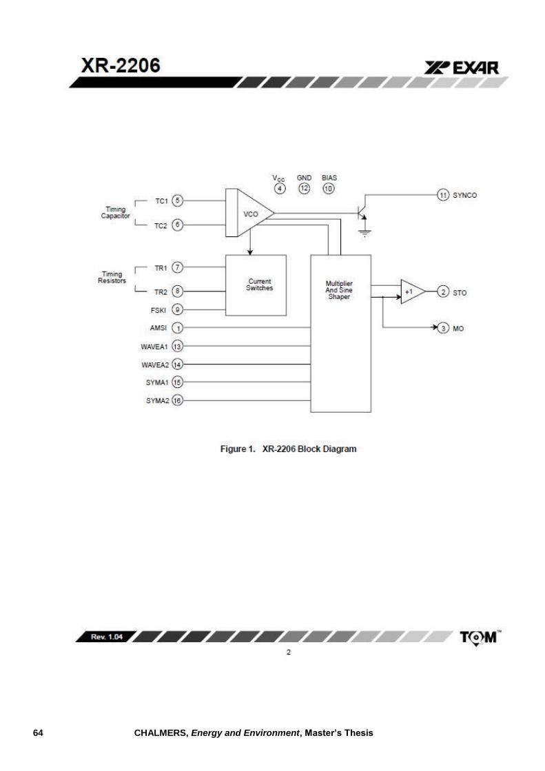
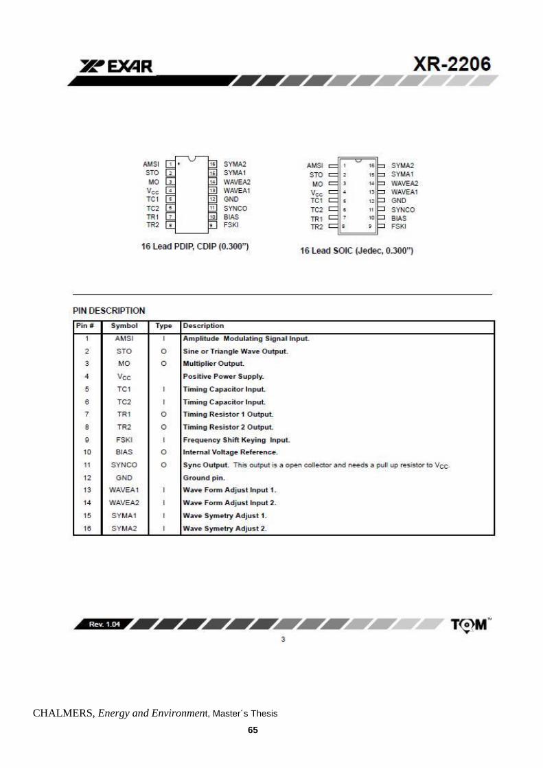
XR2206 Monolithic function generator
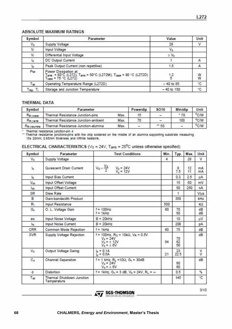
L272M Dual operational amplifier
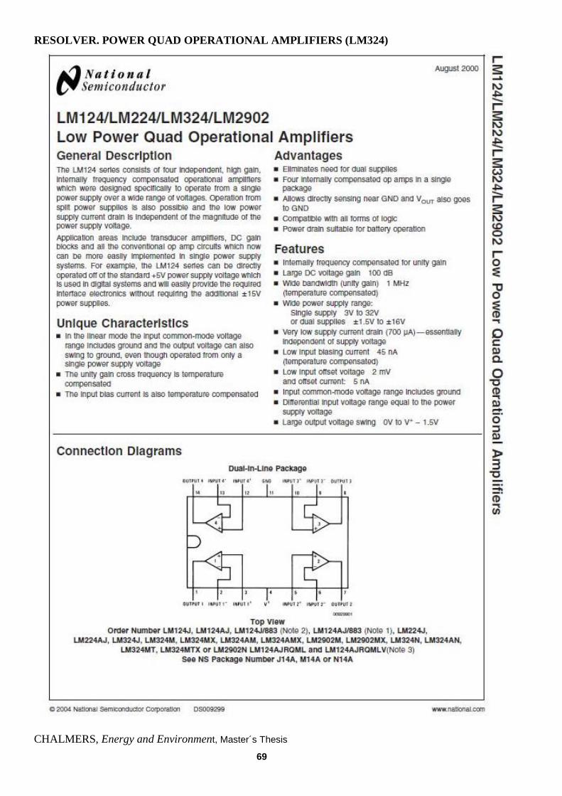
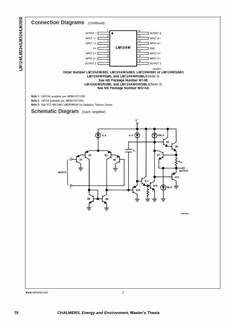
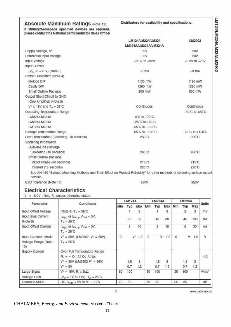
LM234 Low quad operational amplifier
PBC scheme Overall scheme of the PBC
Three-Phase Relay C3 A30 3-phase relay
IRF830 Mosfet for the driving circuit
Below, the data sheet of each component is presented. In some cases, the data sheet of
one component is too extensive, so only the first pages are included. In case of need
of the whole document, it can be found in the web page www.datasheetcatalog.com,
as well as in other similar pages.
Page 62
50 CHALMERS, Energy and Environment, Master’s Thesis
CURRENT PROBE LEM LA 50-S/SP1
Page 63
CHALMERS, Energy and Environment, Master´s Thesis
51
Page 64
52 CHALMERS, Energy and Environment, Master’s Thesis
VOLTAGE TRANSDUCER UMAT2
Page 65
CHALMERS, Energy and Environment, Master´s Thesis
53
Page 66
54 CHALMERS, Energy and Environment, Master’s Thesis
Page 67
CHALMERS, Energy and Environment, Master´s Thesis
55
Page 68
56 CHALMERS, Energy and Environment, Master’s Thesis
RELAY C3-A30
Page 69
CHALMERS, Energy and Environment, Master´s Thesis
57
MOSFET IN RELAY ACTIVATION CIRCUIT (IRF830)
Page 70
58 CHALMERS, Energy and Environment, Master’s Thesis
RESOLVER. RESOLVER-TO-DIGITAL CONVERTER (AD2S83)
Page 71
CHALMERS, Energy and Environment, Master´s Thesis
59
Page 72
60 CHALMERS, Energy and Environment, Master’s Thesis
Page 73
CHALMERS, Energy and Environment, Master´s Thesis
61
Page 74
62 CHALMERS, Energy and Environment, Master’s Thesis
Page 75
CHALMERS, Energy and Environment, Master´s Thesis
63
RESOLVER. FUNCTION GENERATOR (XR-2206)
Page 76
64 CHALMERS, Energy and Environment, Master’s Thesis
Page 77
CHALMERS, Energy and Environment, Master´s Thesis
65
Page 78
66 CHALMERS, Energy and Environment, Master’s Thesis
RESOLVER. DUAL OPERATIONAL AMPLIFIER (L272M)
Page 79
CHALMERS, Energy and Environment, Master´s Thesis
67
Page 80
68 CHALMERS, Energy and Environment, Master’s Thesis
Page 81
CHALMERS, Energy and Environment, Master´s Thesis
69
RESOLVER. POWER QUAD OPERATIONAL AMPLIFIERS (LM324)
Page 82
70 CHALMERS, Energy and Environment, Master’s Thesis
Page 83
CHALMERS, Energy and Environment, Master´s Thesis
71
Page 84
72 CHALMERS, Energy and Environment, Master’s Thesis
Appendix E. dSpace software implementation.
1. Main real-time system.
2. Current and DC bus measurements.
Page 85
CHALMERS, Energy and Environment, Master´s Thesis
73
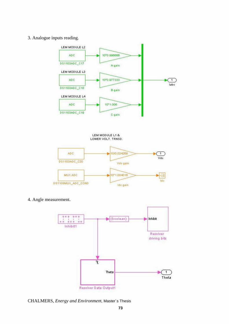
3. Analogue inputs reading.
4. Angle measurement.
Page 86
74 CHALMERS, Energy and Environment, Master’s Thesis
5. Speed calculation.
6. Operations.
Page 87
CHALMERS, Energy and Environment, Master´s Thesis
75
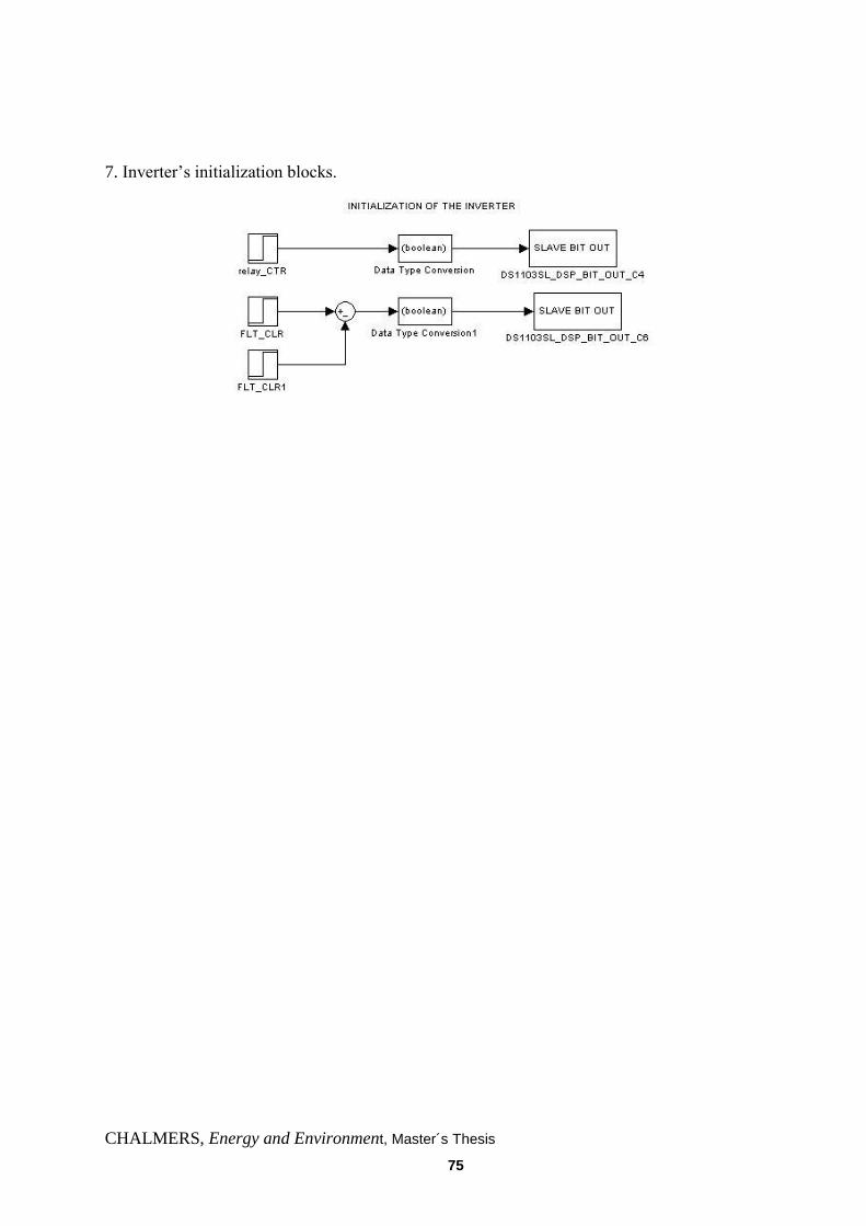
7. Inverter‟sinitializationblocks.


![[G73] PMSM Document](https://static.documents.pub/doc/80x56/5475c6b7b4af9f29698b4589/g73-pmsm-document.jpg)


