1 Pollutant Emissions, Energy Consumption and Economic Development in China: Evidence from Dynamic Panel Data † Bao-shan Zhang a,b,∗ a. School of Economics & Finance, Xi’an Jiaotong University, Xi’an, 710061, China b. Department of Financial and Management Studies, School of Oriental and African Studies, University of London, London, WC1H 0XG, UK Tel: +44 0740 4509 732 E-mail: [email protected];[email protected]Xiao-ling Yuan a a. School of Economics & Finance, Xi’an Jiaotong University, Xi’an, 710061, China E-mail: [email protected]We would like to submit our paper to Oxford Development Studies (ODS). Bao-shan Zhang is a PhD candidate at Xi’an Jiaotong University and a visiting student at SOAS, University of London from 1 September 2009 to 31 August 2010. Dr. Hong Bo is his superviser in UK, she is a Senior Lecturer at Department of Financial&Man, SOAS. Xiaoling Yuan is his superviser in China, she is a professor at School of Economics & Finance, Xi’an Jiaotong University. † The authors are grateful to senior lecturer Hong Bo and professor Bwo-Nung Huang for kindly guarding on econometric methods used in this paper. They are grateful to the third phase “211” Project of Xi’an Jiaotong University for financial support. Bao-shan Zhang also thanks Zhong-nan Huang, Yang Yang, Hsiang-Chun Michael Lin and the Postgraduate Scholarship Program from China Scholarship Council for their supports. Any errors that may remain in this paper are our own. ∗ Corresponding author: Bao-shan Zhang, tel: +44 0740 4509 732 E-mail: [email protected]; [email protected]
Transcript
1
Pollutant Emissions, Energy Consumption and
Economic Development in China: Evidence
from Dynamic Panel Data†
Bao-shan Zhanga,b,∗ a. School of Economics & Finance, Xi’an Jiaotong University, Xi’an, 710061, China
b. Department of Financial and Management Studies, School of Oriental and African Studies, University of London, London, WC1H 0XG, UK
We would like to submit our paper to Oxford Development Studies (ODS). Bao-shan Zhang is a PhD candidate at Xi’an Jiaotong University and a visiting student at SOAS, University of London from 1 September 2009 to 31 August 2010. Dr. Hong Bo is his superviser in UK, she is a Senior Lecturer at Department of Financial&Man, SOAS. Xiaoling Yuan is his superviser in China, she is a professor at School of Economics & Finance, Xi’an Jiaotong University.
† The authors are grateful to senior lecturer Hong Bo and professor Bwo-Nung Huang for kindly guarding on econometric methods used in this paper. They are grateful to the third phase “211” Project of Xi’an Jiaotong University for financial support. Bao-shan Zhang also thanks Zhong-nan Huang, Yang Yang, Hsiang-Chun Michael Lin and the Postgraduate Scholarship Program from China Scholarship Council for their supports. Any errors that may remain in this paper are our own. ∗ Corresponding author: Bao-shan Zhang, tel: +44 0740 4509 732 E-mail: [email protected]; [email protected]
2
Pollutant Emissions, Energy Consumption and Economic Development in China: Evidence from Dynamic Panel Data
Abstract: This study investigates the relationships among pollutant emissions, energy consumption and economic development in China during the period 1982-2007 by using one-step GMM-system model under multivariable panel VAR framework, controlling for capital stock and labor force. Regarding the data for all 28 provinces as a whole, we find that there is a unidirectional positive relationship running from pollutant emission to economic development and a unidirectional negative relationship between pollutant emission and energy consumption. Based on traditional economic planning, the panel data of 28 provinces are divided into two cross-province groups. It is discovered that in the Eastern Coastal region, there is only a unidirectional positive causal relationships leading from economic development to pollutant emission; while in the Central and Western region, there exist the unidirectional Granger causal relationships between pollutant emission and energy consumption, as well as between pollutant emission and economic development. There is also a unique unidirectional causal relationship running from economic development to energy consumption, which does not appear in the Eastern Coastal region or in China as a whole. JEL classification: C33; O53; Q43; Q20 Keywords: GMM-system; Panel VAR; Pollutant emissions; Energy consumption; Economic development; China
3
1. Introduction In 2007, the Intergovernmental Panel on Climate Change (IPCC) reported that the most important environmental problem of our ages is global warming, which is caused by greenhouse gas emissions, especially carbon dioxide (CO2) emissions produced mainly from the consumption of fossil fuels (IPCC, 2007). Due to the increasing threat of global warming, the identification of the relationships among environment pollution, energy consumption and economic development seems to be the priority of handling the greenhouse gas emissions and global warming problems. A deep investigation of pollutant emissions, energy consumption and economic development nexus provides insights in not only the role of energy consumption in economic development, but a basis on which the discussions of energy and environmental policies and economic development strategies are conducted. It is beyond doubt that the linkage between economic growth and energy consumption is of great significance, given that energy, labor and capital are becoming the major sources and development root by increasing and developing national economy, especially for developing countries. The Sixteenth Chinese National Congress (CNC) set a target of four-fold growth of GDP between 2000 and 2020. At the same time, the people’s living standard and per capita national income should reach the level of moderately developed countries, implying that the average annual growth rate of GDP should keep at 7%. To reach the goal, we must ensure that the energy consumption will increase due to the economic growth and the advance in people’s living standard, so will the pollutant emissions. However, there are binding targets about the pollution reduction in “the Eleventh Five-Years Plan”, which was adopted at the Sixteenth CNC. The binding targets are to decrease the GDP energy intensity by 20% and main pollutant emissions by 8% (as to 2005) in 2010.1 Hence, there will be a contradiction between pollutant emissions increase and the desired pollution reduction. The solution to the contradiction is an eager concern of the Chinese government, which also involves the global cooperation on the reduction of greenhouse gases emissions. To solve the problem, we put the factors into a framework to analyze the relationships among them, in order to propose related policies and suggestions for China. China seems to be a good target for an interesting case study, given that it is one of the highest growth economies in the world and it has been experiencing a significant rise in energy consumption with a more serious environmental pollution. China’s rapid economic growth has been associated with a sharp rise in energy consumption which will produce more industrial waste gas emission and waste water discharge. In 2007, China enjoys an average annual economic growth of 11.9% and its real GDP measured in Chinese Yuan with current year price per capita reaches 18, 934.2 Although China is by no means one of the highest growth countries in the world, there is still a great deal of variation in real per capita GDP within its provinces. For example, real per capita GDP data for 2007 ranges from as high as 66, 367 Chinese Yuan per capita in Shanghai
1 Statistics are extracted from the bulletin of Sixteenth Chinese National Congress 2002. 2 Statistics related to annual growth rate, real GDP per capital, energy intensity, and industrial waste gas
emissions per capital are obtained from China Statistical Yearbook 2008.
4
which is located in the developed eastern coastal region to as low as 10, 346 Chinese Yuan per capita in Guizhou,3one of the poorest provinces in China’s less developed western region. In regard to primary energy consumption, the figure for China is 2, 656 million tons standard coal equivalence (SCE) in 2007, while the share of coal in the final energy consumption mix is more than 70%.4 It is clear that coal is still the main energy source for China. However, the consumption and production of coal in 2007 is 2, 586 million tons and 2, 526 million tons respectively,5 which apparently can make a basic balance between them nationwide, while it is hard to make the balance within provinces. Coal is mainly produced in central and western provinces, such as Shanxi, Inner Mongolia, Shaanxi and Henan. The eastern coastal provinces with a stronger economy consume far more than they can produce. For example, Jiangsu, Zhejiang and Guangdong consume 199, 130 and 125 million tons respectively while their production is only 25, 0.12 and 0 million tons.6 With respect to the natural gas, China can basically maintain a balance between demand and supply. In 2007, the production of natural gas is 69, 200 million cubic meter (cu.m), while the consumption of the corresponding time period is 69, 500 million cu.m.7 As for the crude oil, China has become a net importer of crude oil since 1993 and in 2003 it surpassed Japan as the world’s second-largest oil importer (Zhao and Wu, 2007). In addition to the variation in production and consumption within provinces, there is a great deal of variation in the energy intensity as measured by 10 000 Yuan GDP per unit of ton of SCE energy use, ranging from 0.71 in Beijing to 3.95 in Ningxia.8 A fact seen from the analysis above is that China’s rapid economic growth consumes much energy, which will definitely result in large amount of emissions. Adjusting for population and the size of the economy, industrial waste gas emissions measured in ten thousand cu.m per capita ranges from 7.57 in Inner Mongolia to 1.32 in Hainan.9 At the same time, the Chinese central and local governments have set targets about energy saving and emission reduction, whose reduction in 2007 is from a higher -5% in Beijing to a lower -2% in Qinghai.10 China's current task is to solve the contradiction between rapid growth maintaining and greenhouse gas emissions reduction. The choice is also motivated by the fact that China’s energy industries and policy makers face great pressure to change the energy structure and restore with the growing environmental concern among the Chinese people. In light of China’s importance within world economy and energy markets, it is surprising there have been no published methodical empirical studies that explore the relationships among energy consumption, pollutant emission and economic development for China. The task of this paper is to fill the gap in the empirical literature. 3 See footnote 2. 4 All statistics reported on energy consumption and production are obtained from China Energy Statistical
Yearbook 2008. 5 See footnote 4. 6 See footnote 4. 7 See footnote 4. 8 See footnote 2. 9 See footnote 2. 10 Statistics on the target of energy saving and emission reduction is extracted from the 2008 bulletin of National
Development and Reform Commission ( www.sdpc.gov.cn ).
5
This paper is organized as follows: Section 2 is a brief review of related literatures; Section 3 is an introduction of data and methodology; Section 4 discusses and analyzes empirical results; in Section 5 the author posits the policy implications derived from this study; Section 6 ends the paper by providing some concluding remarks.
2. Brief literature review The relationships between economic development and energy consumption, as well as economic development and environmental pollution have been the subject of intense research in the economic literatures over the past few decades worldwide. There are two lines of well-established empirical studies dealing with this nexus. The first line of studies focuses on the relationships between economic development and environmental pollution, and has been well discussed in the hypothesis of Environmental Kuznets Curve (EKC) where environmental degradation initially increases with the level of per capita income, reaches a turning point, and then declines with further increases in per capita income (Shafik and Bandyopadhyay, 1992; Grossman and Krueger, 1995). Although , the EKC hypothesis that linear, as well as quadratic and cubic relationships between per capita income and carbon dioxide emissions, fail to yield unanimous results. The empirical results of Hettige et al. (1992), Panayotou (1993), Cropper and Griffiths (1994), Selden and Song (1994), and Martinez-Zarzoso and Bengochea-Morancho (2004) are consistent with the EKC hypothesis. However, Dinda (2004) and Stern (2004) critique much of the EKC hypothesis, arguing that the causation could run from emissions to income whereby emissions occur in the production process and income increases. Recognizing this point, Dinda and Coondoo (2006) employ a panel data cointegration methodology in a bivariate setting and find mixed results. The second line of studies concentrates on the relationships between economic development and energy consumption. Since the seminal study by Kraft and Kraft (1978), who found a unidirectional Granger Causality running from output to energy consumption for the United States using monthly data during the period 1947-1974, a voluminous empirical literature emerged to examine the causality relationships between economic development and energy consumption. Akarca and Long (1980), Yu and Choi (1985), Erol and Yu (1987a, 1987b), Abosedra and Baghestani (1989), Hwang and Gum (1991), Bentzen and Engsted (1993) has either confirmed or contradicted the results of Kraft and Kraft (1978), which differ in terms of time period covered, countries chosen, econometric techniques employed, and the proxy variables or control variables used in the estimation (see Payne, 2008 for a recent review). The relationships between economic development and energy consumption have been synthesized into four testable hypotheses (Apergis and Payne, 2009a, b). Firstly, the growth hypothesis suggests that energy consumption plays an important role in economic development both directly and indirectly in the aspect of the production process as a complement to labor and capital. It is confirmed that if an increase in energy consumption causes an increase in real GDP whereby the economy is considered energy dependent. Akarca and Long (1979) found a unidirectional Granger
6
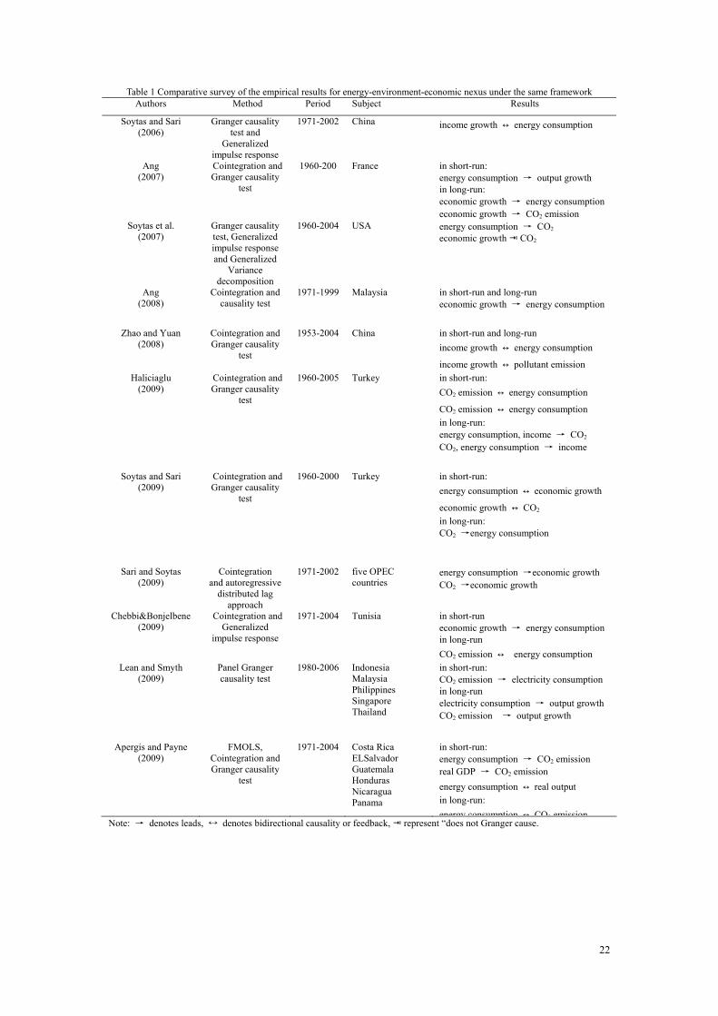
causality running from energy consumption to employment11. Secondly, the conservation hypothesis asserts energy conservation policies designed to reduce energy consumption and waste will not adversely affect real GDP. It is supported by the fact that an increase in real GDP causes an increase in energy consumption. Besides the pioneer study by Kraft and Kraft (1978), which supported the conservation hypothesis, Cheng and Lai (1997) employed Engle-Granger’s cointegration test to investigate the relationships between energy consumption and GDP for Taiwan during 1955-1993. Wietze and Van Montfort (2007) used cointegration analysis to examine the relationships between energy consumption and GDP in Turkey over the period 1970-2003. Both of them discovered a unidirectional causal relationships running from GDP to energy consumption. Thirdly, the neutrality hypothesis considers energy consumption to be a small component of overall output and thus might have little or no impact on real GDP. Hence, under this hypothesis, energy conservation policies would not adversely affect real GDP. It is supported by the absence of causal relationships between energy consumption and real GDP. Akarca and Long (1980), Erol and Yu (1987a, 1987b, 1989), Yu and Hwang (1984), Yu and Chio (1985), Yu et al. (1988), Yu and Jin (1992), Altinay and Karagol (2004) found no causal relationships between the two. The neutrality hypothesis is therefore established. Finally, the feedback hypothesis suggests that energy consumption and real GDP are interrelated and might very well serve as complements to each other. It is supported by the bidirectional causal relationships between energy consumption and real GDP, with the implication that an energy policy oriented toward improvements in energy consumption efficiency would not adversely affect real GDP. Employing Engle-Granger’s cointegration method along with FPE of Hsiao (1981), Yang (2000) discovered a bidirectional between energy consumption and economic development. Paul and Bhattacharya (2004) also found bidirectional causality between energy consumption and economic development. With advances in econometric techniques, more recent studies tend to focus on cross-section countries with panel data (Masih and Masih, 1996; Asafu-Adjaye, 2000; Soytas and Sari, 2003; Lee, 2005, 2006; Lee and Chang, 2007and 2008; Narayan and Smyth, 2008; Apergis and Payne, 2009a, 2009b). However, these empirical studies on the relationships between energy consumption and economic development still yield mixed results as to the aforementioned hypothesis.The existing literatures reveal that the empirical studies differ substantially and are not conclusive to present policy recommendation which can be applied across countries (Chebbi and Boujelbene, 2009). Given that energy consumption has a direct impact on the level of environmental pollution, the above discussion clearly highlights the importance of linking these two strands of literatures together (Ang, 2007). It is not until recently when scholars began to investigate the relationships among energy consumption, pollutant emissions and economic development under the same framework. Table 1 lists some of the most recent studies which pertain to energy-environment-
11 In the literature, some economists use employment or production to substitute for economic growth.
7
economic nexus. With the exception of Sari and Soytas (2009) and Lean and Smyth (2009), all of the studies primarily focus on single countries. Few papers include labor force and capital stock as controlled variables in their models. The results from these studies, however, are still mixed. Ang (2007) found unidirectional Granger causality running from economic growth to energy consumption in the long-run and running from energy consumption to economic growth in the short-run. At the same time, Soytas and Sari (2009) found unidirectional Granger causality running from carbon emissions to energy consumption in short-run and no causality relationships between economic growth and carbon emissions in the long-run, implying that the reduction in carbon emissions does not have to forgo economic growth in Turkey. Apergis and Payne (2009a) found unidirectional causality from energy consumption and real output, respectively, to emissions along with bidirectional causality between energy consumption and real output in short-run and bidirectional causality between energy consumption and carbon dioxide emissions in the long-run for six Central American countries. However, Sari and Soytas (2009) reached the conflicting results for five OPEC countries. This paper is unlike earlier ones in the sense that it compares the relationships among energy consumption, economic development and pollutant emissions, controlling for capital stock and labor force in China with a provincial panel data. Table1 here In both lines of research, the bulk of the work was on developed countries, and there are even a more limited number of empirical researches which investigate the relationships between economic development and energy consumption or between economic development and environmental pollution in China. It is interesting that there has so far been little effort attempting to examine the relationships between energy consumption and carbon dioxide emissions. Cole et al. (2008) used industry-level data during the period of 1997-2003 to examine the determinants of environmental pollution for China, and found that energy consumption had a positive impact on industrial pollution whereas productivity improvements and research activities tend to reduce emission. For more detailed discussions on pollutant emissions and carbon dioxide emissions in China, please refer to Ang (2009). To the extent of our knowledge, only Soytas and Sari (2006) and Zhao and Yuan (2008) deliberatively examined the relationships between energy consumption, carbon dioxide emissions and economic growth in China under an integrated framework. Soytas and Sari (2006) found no long-run Granger causality between energy consumption and economic growth, implying that energy conservation or energy shortage might not hamper Chinese economic growth in the long-run; however, carbon dioxide emissions series is omitted in their empirical model. Zhao and Yuan (2008) found bilateral causality running between income growth with energy consumption and pollutant emissions, both in the short-run and long-run. Based on the panel data, the author attempts to examine the relationships between pollutant emissions, energy consumption and economic development under a multivariate and integrated framework, which seems to be a relatively new area of research. In order to compensate for the deficiency in an inadequate sample size caused by short data span, the panel data approach is needed to reevaluate the relationships between pollutant emissions, energy consumption and economic development in China. Following the idea of Apergis and Payne (2009a, b), Lean and Smyth (2009) and Huang et al. (2008), we investigate the dynamic relationships between pollutant emissions, energy consumption and economic development with a provincial panel data for China, accounting for possible affects of labor force and capital stock. However, the use of panel data
8
also creates another problem the dynamic heterogeneity of the panel data. Yuan et al. (2008) point out that different countries are in utterly different developing stages and developing process might have significantly different impact on energy consumption and economic growth relation. Furthermore, Soytas and Sari (2007) also point out that different countries have different energy consumption and various sources of energy, which might have varying impacts on the economic growth and pollutant emissions. Therefore, we classify the panel data into two sub-panels based on economic development level and conventional regionalization of economy layout before further estimation, which is another contribution of this paper to resolve the “lump-together” problem in using panel data. Also, this empirical country study might be of great use to formulating policy recommendations in energy saving and pollutant emission reduction.
3. Data and methodology 3.1 Data Our study uses annual time series for 28 provinces of China12 with the samples including Beijing, Tianjin, Hebei, Shanxi, Inner Mongolia, Liaoning, Jilin, Heilongjiang, Shanghai, Jiangsu, Zhejiang, Anhui, Fujian, Jiangxi, Shandong, Henan, Hubei, Hunan, Guangdong, Guangxi, Sichuan, Guizhou, Yunnan, Shaanxi, Gansu, Qinghai, Ningxia, Xinjiang. The real GDP (lrgdppc) per capita in terms of Chinese Yuan based on 2000 price index is used as a proxy for the economic development. The data are obtained from National Statistics Bureau of China. The kilograms of SCE per capital are used as a proxy for the energy consumption (lecpc). The data are sourced from National Statistics Bureau of China and China energy CD data book published by Lawrence Berkeley National Laboratory. This paper is unlike earlier ones in the sense of using carbon dioxide emissions as the proxy for the level of pollution. We use total volume of industrial waste gas emission per capita as a proxy for the level of pollution and environmental degradation (lpepc). Industrial waste gas emission refers to the discharge into atmosphere of waste air containing pollutants generated from fuel burning and production processes, which represents the level of pollutant emissions better than carbon dioxide emission does. The unit is expressed in 10 thousands cu.m. Labor force (ll) and capital stock (lk) are two controlled variables. The labor force is collected from China Compendium of Statistics (1949-2004) and China Center for Economic Research database. Data on capital stock is not available, because of the absence of officially published data. Fortunately some scholars (Zhang et al., 2007; Shan, 2008) specializing in the study of Chinese Capital Stock Estimation follow the capital stock of all provinces in China and provide open data. In this paper, capital stock data are sourced from the open data published in the Journal of Quantitative and Technical Economics13. All variables are converted into natural logarithms, so that they can be interpreted in growth terms after taking first differences. The data span 26 years from 1982-2007 including 28 provinces. Among these 28 provinces, 11 provinces are classified as Eastern provinces, and 17 provinces are Central and Western provinces. 12 The provinces of Hainan, Chongqing, Tibet and Taiwan, as well as Hong Kong and Macao Special Administrative Regions are not included in our study, because of the lack of the original source data. 13 The Journal of Quantitative and Technical Economics is a Chinese economics journal.
9
3.2 Econometric methodology Our empirical estimation has two objectives. The first is to examine how the variables are related. The second is to investigate the dynamic causal relationships between the variables. In the time series data, the Granger causality test is usually employed to examine the causal relationships between variables. However, the dynamic panel estimation approach needs to be used to identify the causal relationships for the panel data variable. Following the framework of Huang et al. (2008) and Lee and Chang (2007), we construct a five-variable panel-VAR model for the estimation purpose. In a panel of N provinces covering T years, our five-variable vector auto-regressions taking into consideration the individual fixed effects have the following form:
1
, , , ,1
( )p
i t j i t j i t i t i tj
y y L xα β η φ ε+
−=
′= + + + +∑ (1)
where the subscripts are ith province and tth period. ,i ty is ,i tlrgdppc , or ,i tlecpc , or ,i tlpepc
for province i at time t; ,i tx are predetermined variables as ,i t jll − , ,i t jlk − , ,i t jlrgdppc − ,
,i t jlecpc − , or ,i t jlpepc − , where 1, ,j p= L . p is an optimal lag period; ( )Lβ is a
polynomial lag operator; iη is a province-specific fixed effect14, which capture all fixed inherent
to each province, such as geographical, social and local policy province aspects; tφ is a
time-specific effect, which captures productivity, regulatory or economic changes that are
common to all provinces; ,i tε is a random disturbance and assumed to be independently
distributed with zero mean, but arbitrary forms of heteroskedasticity across units and times are possible. Applying traditional procedures to estimate equation (1) is unsuitable and will provide biased estimates due to the correlation between the lagged dependent variables and the province-specific
effect, which is , 1( , ) 0i t iE y η− ≠ . Holtz-Eakin et al. (1988) and Arellano and Bond (1991) propose
an alternative approach, where first differences in the regression equation (1) are taken to remove
the province-specific effects iη , so we take the first difference in equation (1) as :
, , , ,1
* ( )p
i t j i t j i t t i tj
y y L xα β φ ε−=
′Δ = Δ + Δ + Δ + Δ∑ (2)
Where Δ is the first-difference operator. Substantial problems rise in the estimation of equation (2), because of the correlation between the
14 we prefer to use a fixed effects specification over a random effects specification, because of system variables are regarded as exhibiting trending behavior.
10
lagged dependent variables and the error term, which is , ,( , ) 0i t j i tE y ε−Δ Δ ≠ . Arellano and Bond
(1991) employed lagged dependent variables ( ,i t sy − for 2s ≥ ) in level as instrument in the
Generalized Method of Moment (GMM) to overcome the problem of , ,( , ) 0i t j i tE y ε−Δ Δ ≠ . Then,
the corresponding optimal instrument matrix iZ with predetermined regressors ,i tx correlated
with the individual effect is given by
,1 ,1 ,2
,1 ,1 ,2 ,3
,1 , 2 ,1 , 1
0 0 0 0 0 0 0 00 0 0 0 0 0 0
0 0 0 0 0 0 0
i i i
i i i ii
i i T i i T
y x xy x x x
Z
y y x x− −
⎛ ⎞⎜ ⎟⎜ ⎟= ⎜ ⎟⎜ ⎟⎜ ⎟⎝ ⎠
L L L
L L L
M M M M M M M M M M M
L L L
(3)
Where rows correspond to the first-difference equation (2) for periods 3,4, ,t T= K for
individual i , which exploit the moment conditions
[ , ] 0i iE Z ε′ Δ = for 1, 2, ,i N= K (4)
where ,3 ,4 ,( , , , )i i i i Tε ε ε ε ′Δ = Δ Δ ΔK . In general, the asymptotically efficient GMM estimation
based on this set of moment conditions minimizes the criterion.
1 1
1 1( ) ( )N N
iN i i N ii i
J Z W ZN N
ε ε= =
′ ′= Δ Δ∑ ∑ (5)
Using the weight matrix 1
1
1[ ( )]N
iN i i ii
W Z ZN
ε ε −
=
′′= Δ Δ∑
Where the iεΔ are consistent estimates of the first-differenced residuals obtained from a
preliminary consistent estimator. Hence, this is known as a two-step GMM estimator. Under the
assumption of homoskedasticity ,i tε , the particular structure of the first-differenced model
implies that an asymptotically equivalent GMM estimator can be obtained in one-step, using instead the weight matrix
1
1
1[ ( )]N
iN ii
W Z HZN
−
=
′= ∑
Where H is a (T-2) square matrix with 2’s on the main diagonal, -1’s on the first off-diagonals and
zeros elsewhere. Notice that 1NW does not depend on any estimated parameters15.
Although the one-step estimator is asymptotically inefficient relative to the two-step estimator,
15 This part of the discussion on GMM methodology is mainly based on Bond (2002).
11
simulations suggest that asymptotic inferences based on the one-step estimators are more reliable and have the correct empirical level, while asymptotic inferences based on the two-step estimators can be seriously misleading, and tend to reject the null hypothesis too frequently, and simulation studies also review that very modest effiency gains from using the two-step version, even in the presence of considerable heteroskedasticity (Arellano and Bond, 1991; Blundell and Bond, 1998; Blundell et al. , 2000). Hence, in our estimation, the robust one-step estimator is employed. The GMM-difference estimator can successfully handle endogeneity, measurement errors and omitted variables problems for the dynamic panel model. However, the GMM-difference estimator is not suitable in all circumstance. Blundell and Bond (1998) pointed that the GMM estimator in the first difference model shows bias problems when variables are persistent, which is the case of pollutant emissions, economic development and energy consumption variables. Under this circumstance, the instruments used in the GMM-difference estimator have been proven to be weak and the first difference estimator is poorly behaved. Therefore the key difference between the GMM-difference and GMM-system lies in the treatment of instruments. Whereas the former
approach uses iZ (lagged levels) in the difference equations, the latter estimator uses
*iZ (lagged differences) in the level equations, *iZ is defined as follows:
2
3
, 1
0 0 00 0 0
* 0 0 0
0 0 0
i
i
i i
i T
Zy
Z y
y −
⎛ ⎞⎜ ⎟Δ⎜ ⎟⎜ ⎟= Δ⎜ ⎟⎜ ⎟⎜ ⎟Δ⎝ ⎠
L
L
L
L
(6)
Because of the good performance of the GMM-system estimator relative to the GMM-difference estimator in terms of weak instruments problem, it has become the estimator of choice in many applied panel data setting and it is beginning to be used in recent years in the areas such as economic growth (Caselli et al., 1996; Benhabib and Spiegel, 2000; Easterly et al., 1997; Forbes, 2000; and Levine et al., 2000), production functions and technological spillovers (Levinsohn and Petrin, 2003; and Griffith et al., 2006). However the GMM-system approach has not been widely used to investigate the relationships between pollutant emissions, energy consumption and economic development in the literature. To our knowledge, there are only two studies on that relationships. Lee and Chang (2007) estimate a panel-VAR using the GMM approach and find evidence of causality from GDP to energy consumption for 18 developing countries and bidirectional causality for 22 developed countries. Huang et al. (2008) employed the GMM-system techniques to estimate panel-VAR model for the relationships between energy consumption and GDP growth of 82 countries; based on income levels, the sample is devided into four groups and different results are reported depending on group considered. It is, therefore, necessary that the GMM-system should be used to investigate the dynamic relationships between pollutant emissions, energy consumption and economic development under a integrated framework. As such, this is one of our major contributions.
12
In terms of model specification, the Sargan test is subjected to check the validity of the instruments used, because of that for a given sample size of cross sections, using too many instruments might result in verifying bias. After the equation is estimated, a simple Wald test can be applied to examine the direction of the causal relationships between pollutant emissions, energy consumption and economic development.
4. Analysis and discussion of results 4.1 Results of the whole country Before estimation, an optimal lag period p should be determined first. There are two approaches to indentify the optimal lag period under the panel VAR model. One is the likelihood ratio test suggested by Holtz-Eakin et al. (1988). Lee and Chang (2007) used the likelihood ratio
test to select the optimal lag period for the estimation of panel VAR. The other one is jm
statistics suggested by Arellano and Bond (1991), where j is the order of autocorrelation. The jm
statistics is based on the standardized average residuals autocovariance, which are asymptotically N (0, 1) distributed under the null hypothesis of no autocorrelation. Huang et al. (2008) and
Marrero (2009) employed the jm statistics to determine the appropriate optimal lag under the
panel VAR model. Huang et al. (2008) also point out that the advantage of using jm statistic test
for an optimal lag is that the panel VAR model will also be free of misspecification from serial correlation with the optimal lag. Table 2 shows the Sargan test results, m1 and m2 statistics, and the results of one-step GMM system estimation under the panel VAR model in China.
Table 2 here As m1 and m2 statistics in Table 2 show, the selection of the two lag periods for the economic development equation, three lag periods for the energy consumption equation, and a delay of one period for pollutant emission equation are needed for the panel in order to satisfy the assumption of no serial correlation in the disturbances. In fact, significant negative first order serial correlation is found in the first differenced residuals, while there is no evidence of second order serial correlation. Furthermore, the Sargan test statistics indicate that we do not reject the validity of the instruments, that is, the instrument variables used in the one step GMM system estimation of our panel VAR model are appropriate. In terms of Granger causality test, we observe from the Table 2 that there are only two significant results. One of the results indicates that we reject the null hypothesis that pollutant emission does not Granger cause economic development at the 5% significance level, and the reverse does not hold, since the causality is not bi-directional. The estimated results of economic development equation further reveal that the effect of pollutant emission on economic development is positive (the coefficient for two period lag is 0.0272, although the coefficient for one period lag is not significant statistically). In other words, continued pollutant emission increase, accompanied by a rise in economic development. This situation might be coincided with the facts that the
13
tremendous achievements in China’s economic development is at the expense of the environment and resources. Further, given the Environmental Kuznets Curve (EKC) hypothesis, it also manifestos that China is still on the left side of the peek of EKC. Interestingly, another result reveals that there is evidence of a unidirectional causality running from industrial waste air emission to energy consumption. The industrial waste air emission mainly consists of CO2, SO2 and NO2, which produced in the course of energy consumption. There is no doubt expecting the causal relationships leading from energy consumption to pollutant emission. This might be arising due to the fact that pollution emissions increasing results from the huge energy consumption. However, more efficient use of energy and more investment in environmental pollution could result in a reduction in pollutant emission. The increasing costs of environmental pollution control in China indicate that China doesn’t want to follow the developed countries “treatment after pollution” road. Therefore, the fact is that China is a developing country while making more efforts on environmental pollution control. In 2007, the investment for environmental pollution treatment in the whole country hit 110.66 billion Yuan, 4.3% over the previous year. The test results also indicate that there are no causal relationships between economic development and energy consumption. On the one hand, the Walt test of energy consumption is not significant in economic development equation. On the other hand, the Walt test of economic development is not significant in energy consumption equation. In other words, an increase in energy consumption does not lead economic development and an increase in economic development does not bring an increase in energy consumption. This is not good news for energy policymakers. However, according to Granger causality test, if X Granger causes Y, it is simply implying that X contains useful information for predicting Y. Hence, we use the concept of causality in the predictive rather than in the deterministic sense in this paper. Therefore, we can conclude that past energy consumption does not help to predict economic development, and, analogously, past economic development does not help to predict energy consumption. Therefore the neutrality hypothesis is established. 4.2 Results of different groups Attempting to create a stable, prosperous and highly competitive (or more energetic) country, China has adopted many regional development strategies of promoting balanced development among different regions since 1997, such as the strategy of Western Development Drive, the strategy of Rejuvenation of Northeast Old Industrial Base, and the Strategy of Rising in Central Region. There are four important and well organized economic regions in China: Eastern Coastal region, Central region, Western region and Northeast region. Besides a strong economic relationships due to a close geographical position, these regions enjoy the same preferential tax policy in investment, as well as the policy of energy saving and emission reduction. In this paper, we broaden the scope of our study by dividing China into two cross-regional groups, which are the Eastern Coastal region and Central and Western region in order to gain better understanding of the relationships between pollutant emission, energy consumption and economic development for China different regions.
14
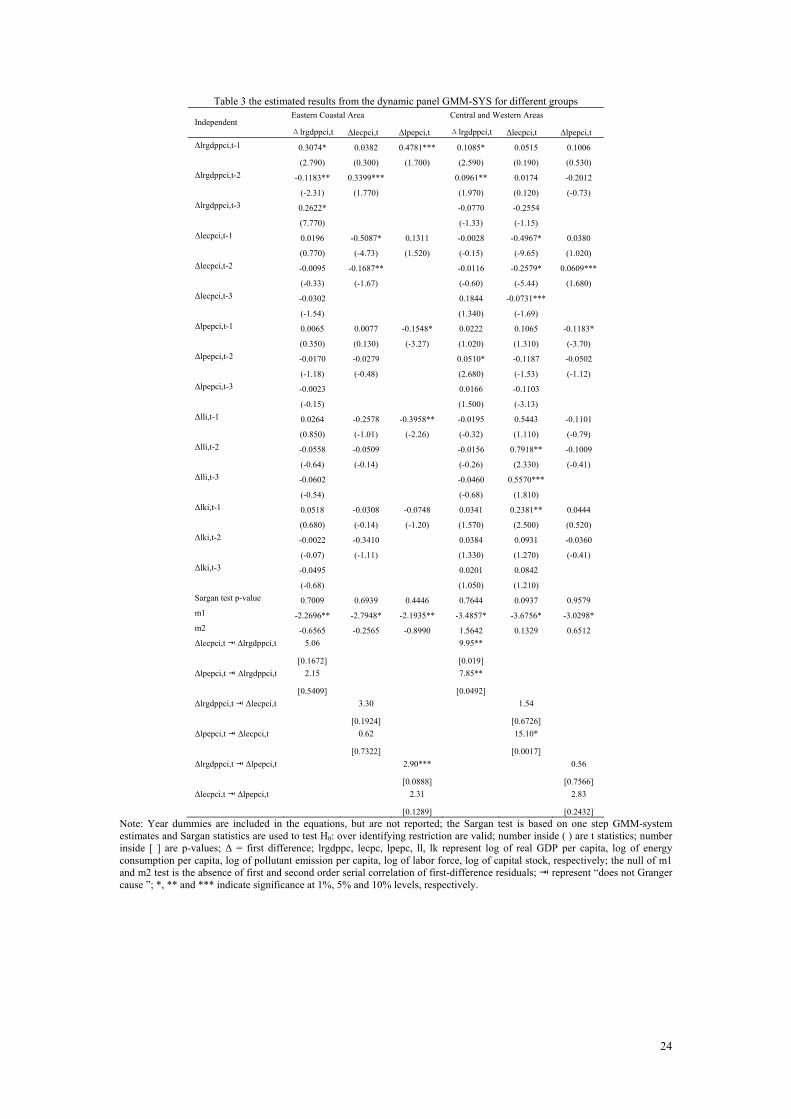
Furthermore, the disadvantage of using panel data is another reason for this dividing. All 28 provinces, as a whole, are treated as a unit, neglecting the difference among provinces or regions16.
Table 3 here The estimated results for the two different groups are reported in Table 3. The m1 and m2 statistics of Table 3 indicate that there are no serial correlations in the disturbances. The selection of the three lag periods is needed for economic development equation in Eastern Coastal region and energy consumption equation in Central and Western region in order to satisfy the assumption. For the energy consumption equation in Central and Western region and economic development equation in Eastern Coastal region, the use of VAR(2) is sufficient. The pollutant emission equation for the two different groups require a lag of 1 and 2 periods in order to rid the serial correlation of panel VAR residuals. Further, in all models, the Sargan statistics indicate that we cannot reject the null hypothesis and the instrument variables are appropriate in our estimation. For the Eastern Coastal region, the absence of Granger causality between energy consumption and economic development, or between energy consumption and pollutant emission, indicates that energy consumption does not lead to economic development and an increase in economic development also does not bring an increase in energy consumption, just the same causal relationships as China treating as a whole, and so does the same to energy consumption and pollutant emission. Given that a great deal of waste pollutant emission produced in energy use production, there will be doubt that why energy consumption is not Granger cause of pollutant emission. It might indicate that industrial waste gas emissions, which represent for the level of pollution and environmental degradation, might be a part of total or real pollutant emission in China, there might be another major portion of the pollutant emission, the data of which is hard to be obtained, such as the excessive biomass use for heating and cooking by the rural households. Jiang and Q’ Neill (2004) pointed out that 63% of households still use biomass for heating and cooking, which accounts for more than 70% of total fuel use among the China rural population. For the relationships between economic development and pollutant emission, the Granger causality shows that the pollutant emission does not Granger cause to economic development, but an increase in economic development might bring an increase in pollutant emission at the 10% significance level. Production goes with emissions. However, the changes in pollution aren’t the reason for economic growth. Citations explain that the source of economic growth in developing countries is mainly based on neo-classical economics model, i.e., capital accumulation and labor inputs cause economic growth. For the Central and Western region, we have causal relationships between energy consumption and pollutant emission and between energy consumption and economic development, similar to China as a whole. Take pollutant emission and energy consumption for example, an increase in 16 The national income level representing economic development is often used in the empirical literature to
classify panel data into different groups (De Gregorio and Guidotti, 1995; Bwo-Nung Huang, 2008). If we classify
China into two groups (Eastern Coastal region, as well as Central and Western region) based on income level, the
results is consistent with traditional economic region. So, in this paper, we take two cross-provincial groups to
have a deep investigate for the nexus of environment-energy-economic development.
15
energy consumption does not bring about pollutant emission, and vice versa. There is a unique causal relationship between energy consumption and economic development according to our empirical studies. That is the unidirectional causal relationships running from economic development to energy consumption, but not vice versa. The findings of Granger causality relationships between pollutant emission, energy consumption and economic development from our empirical studies might have important implications for China’s economy. In the light of our empirical results, the next section briefly discusses the policy implications.
5. Policy implications In consideration of the high economy and energy consumption growth rate, as well as high industrial waste gas emission growth rate, the environment-energy-development nexus poses tremendous challenges to Chinese policy makers. Economic growth rate is expected to keep as high as 7%-8% in the next two decades (Zhao and Yuan, 2008) and China has set ambitious targets in reducing so called carbon intensity (the amount of carbon dioxide emitted per unit of economic output) by 40%-45% by 2020 compared with 2005 levels . There is a simple cost-benefit relationship generalized from the Granger causal relationships between pollutant emission, energy consumption and economic development. Along with economic development, energy consumption will bring about the externality of environmental pollution. The question is whether energy consumption can result in greater benefits in economic development relative to the cost of environmental pollution (Huang, 2008). Some critical policy implications emerge from our findings. However, the most important policy implication derived from our empirical study might be that we should take the degree of economic development into consideration when energy policy is formulated for each province. The one-size-for-all energy policy in China is not appropriate for it fails to implement correct policies for different provinces in different economic development levels. There is a unidirectional Granger causality running from pollutant emission to economic development positively both in China as whole and in Central and Western region. It is not surprising that in China an increase in pollution level induces economic growth. From the basic cost-benefit point of view, as the economy increases, the energy consumption will increase, but the externality of environmental pollution from the over-use in energy is greater than the benefit it brings. From a practical point of view, energy inputs have been consumed in the production to promote heavy industry (the gross value of industrial output of heavy industry accounted for 70.47% of the whole country in 2007). As Ang (2008) points out that a persistent decline in environmental quality might exert a negative externality to the economy through affecting human health, and thereby decrease economic development. Our policy suggestions are that, effective measures need to be carried out to optimize its industrial structure and reduce the share of coal in total energy consumption. Since coal emits twice as much carbon dioxide as natural gas,
16
sustainable coal technologies should be imposed on the heavy industry enterprise and coal power plants with carbon dioxide capture and storage facilities. On the other hand, feasible measure is to promote energy efficiency and increase energy investment. For the Eastern Coastal region, our empirical results indicate that pollutant emission tends to increase following economic development. For this reason, it seems possible that an energy conservation policies could be achieved though the reduction of energy consumption without impact on economic development. For the provinces belonging to Central and Western region, our empirical study reveals that energy consumption leads to economic development. The implication is that energy conservation measures might be implemented but with some effect on economic growth in Central and Western region’s provinces.
6. Conclusions and remarks The study of causal relationships between pollutant emissions, energy consumption and economic development in China when capital stock and labor force variables are controlled for is certainly of considerable interest in terms of designing appropriate energy policies and development strategy. In this paper, we investigate the dynamic linkages between environments-energy- development for China during the period 1982-2007 using one-step GMM-system model under a five variables panel VAR framework. We use the panel data of 28 provinces and classify the data into two groups based on traditional economic planning without such a classification the difference among provinces and regions will be neglected. Regarding the data for all 28 provinces as a whole, we find that there are unidirectional positive relationships running from pollutant emission to economic development and unidirectional negative relationships between pollutant emission and energy consumption. After the data are classified into two groups, the Granger causal relationships in each group are fairly different. For the Eastern Coastal region, there is only a unidirectional positive causal relationship leading from economic development to pollutant emission. For the Central and Western region, the unidirectional Granger causal relationships between pollutant emission and energy consumption, as well as between pollutant emission and economic development are found. There is also a unique unidirectional causal relationship running from economic development to energy consumption, which does not appear in the Eastern Coastal region or China as whole. It is apparent that the classification of 28 provinces into two different groups is effective to better understand the causal relationships between environment-energy- development and more useful for energy policy makers. The main contribution of this paper is that for the first time an attempt is made to investigate the relationship between pollutant emission, energy consumption and economic development for China during the period of 1982-2007 employing a multivariable panel VAR model along with one step GMM-system estimation. Although the finding from our empirical study might be unique to China due to its social and economic background and development approach, the methodology employed in this study can be readily extended to other developing countries for their energy policy making and strategy of economic development formulating. However, the empirical results are very helpful in making clear understanding of the current dynamic relationships between
17
pollutant emissions, energy consumption and economic development in China and also revealing the tasks and direction of further research. In this paper, we use total volume of industrial waste gas emission per capita as a proxy for level of pollution and environmental degradation, which might be worthwhile for future work to take carbon dioxide emission from Chinese rural area by heating and cooking and straw-returned after harvest into account as well. Since China is facing an investment and technology problem, financing for energy investment and energy investment behavior analysis need to be further investigated. It is hoped that these lines of research will be useful for Chinese energy saving and pollutant emission reduction, thus making contribution on GHG (Greenhouse Gases) emission reduction.
18
References Abosedra, S., Baghestani, H., 1989. New evidence on the causal relationship between United
States energy consumption and Gross National Product. Journal of Energy and Development 14, 285-392.
Akarca, A.T., Long, T.V., 1979. Energy and employment: a time series analysis of the causal relationship. Resources Energy 2, 151-162.
Akarca, A.T., Long, T.V., 1980. On the relationship between energy and GNP: a reexamination. Journal of Energy and Development 5, 326-331.
Altinay, G., Karagol, E., 2004. Structural break, unit root, and the causality between energy consumption and GDP in Turkey. Energy Economics 26, 985-994.
Ang, J.B., 2007. CO2 emissions, energy consumption and output in France. Energy Policy 35, 4772-4778.
Ang, J.B., 2008. Economic development, pollutant emissions and energy consumption in Malaysia. Journal of Policy Modeling 30, 271-278.
Ang, J.B., 2009. CO2 emissions, research and technology transfer in China. Ecological Economics 68, 2658-2665.
Apergis, N., Payne, J.E., 2009a. Energy consumption and economic growth in Central America: evidence from a panel cointegration and error correction model. Energy Economics 31, 211-216.
Apergis, N., Payne, J.E., 2009b. Energy consumption and economic growth: evidence from the Commonwealth of Independent States. Energy Economics 31, 641-647.
Arellano, M., Bond, S., 1991. Some test of specification for panel data: Monte Carlo evidence and an application to employment equations. Review of Economic Studies 58, 277-297.
Asafu-Adjaye, J., 2000. The relationship between energy consumption, energy prices and economic growth: time series evidence from Asian developing countries. Energy Economics 22, 615-625.
Benhabib, J., Spiegel, M.M., 2000. The role of financial development in growth and investment. Journal of Economic Growth 5, 341-360.
Bentzen, J., Engsted, T., 1993. Short- and long-run elasticities in energy demand : a cointegration approach. Energy Economics 15, 9-16.
Blundell, R., Bond, S., 1998. Initial conditions and moment restrictions in dynamic panel data models. Journal of Econometrics 87, 115-143.
Blundell, R., Bond, S., Windmeijer, F., 2000. Estimation in dynamic data models: improving on the performance of the standard GMM estimator. Working Paper. The Institute for Fiscal Studies.
Caselli, F., Esquivel, G., Lefort, F., 1996. Reopening the convergence debate: a new look at cross-country growth empirics. Journal of Economic Growth 1, 363-389.
Chebbi H.E., Boujelbene, 2009. CO2 emissions, energy consumption and economic growth in Tunisia. 2008 International Congress, August 26-29, 2008, Ghent, Belgium 44016, European Association of Agricultural Economists.
Cheng, B.S., Lai, T.W., 1997. An investigation of co-integration and causality between energy consumption and economic activity in Taiwan. Energy Economics 19, 435-444.
Cole, M.A., Robert E.J.R., Shanshan, W., 2008. Industrial activity and the environment in China:
19
an industry-level analysis. China Economic Review 19, 393-408. Cropper, M., Griffith, C., 1994. The interaction of population growth and environmental quality.
American Economic Review 84, 250-254. Department of Comprehensive Statistics of National Bureau of Statistics, 2005. China
Compendium of Statistics (1949-2004). China Statistics Press, Beijing. Dinda, S., 2004. Environmental Kuznets curve hypothesis: a survey. Ecological Economics 49.
431-455. Dinda, S., Coondoo D., 2006. Income and emission: a panel data based cointegration analysis.
Ecological Economics 57, 167-181. Easterly, W., Loayza, N., Montiel, P., 1997. Has Latin America’s post-reform growth been
disappointing?. Journal of International Economics 43, 287-311. Erol, U., Yu, E.S.H., 1987a. On the causal relationship between energy and income for
industrialized countries. Journal of Energy and Development 13, 113-122. Erol, U., Yu, E.S.H., 1987b. Time Series analysis of the causal relationship between U.S. energy
and employment. Resources and Energy 9, 75-89. Erol, U., Yu, E.S.H., 1989. Spectral analysis of the relationship between energy and income for
industrialized countries. Resources and Energy 11, 395-412. Forbes, K., 2000. A reassessment of the relationship between inequality and growth. American
Economic Review 90, 869-887. Griffith, R., Harrison, R., Reenen, J.V., 2006. How special is the special relationship? Using the
impact of U.S. R&D spillovers on U.K. firms as a test of technology sourcing. The American Economic Review 96, 1859-1875.
Grossman, G.M., Krueger, A.B., 1995. Economic growth and the environment. Quarterly Journal of Economics 110, 353-377.
Haliciaglu, F., 2009. An econometric study of CO2 emissions, energy consumption, income and foreign trade in Turkey. Energy Policy 37, 699-702.
Hettige, H. Lucas, R.E.B., Wheeler, D., 1992. The toxic intensity of industrial production: global patterns, trends and trade policy. American Economic Review Papers and Proceedings 82, 478-481.
Holtz-Eakin, D., Newey, W., Rosen, H.S., 1988. Estimating vector autoregressions with panel data. Econometrica 56, 1371 - 1395.
Hsiao, C., 1981. Autoregressive modeling and money income causality detection. Journal of Monetary Economics 7, 85-106.
Huang, B.N. Hwang, M.J., Yang, C.W., 2008. Causal relationship between energy consumption and GDP growth revisited: a dynamic panel data approach. Ecological Economics 67, 41-54.
Hwang, D.B.K., Gum, B., 1991. The causal relationship between energy and GNP: the case of Taiwan. Journal of Energy and Development 16, 219-226.
Intergovernmental Panel on Climate Change (IPCC), 2007. Climate change 2007: Synthesis report. Contribution of Working Groups I, II and III to the Fourth Assessment Report of the Intergovernmental Panel on Climate Change. [Core Writing Team, Pachauri, R. K. and Reisinger, A. (eds.)]. IPCC, Geneva, Switzerland.
Jiang, L.W., O’Neill, B., 2004. The energy transition in rural China. International Journal of Global Energy Issues 21, 2-26.
Kraft, J., Kraft, A., 1978. On the relationship between energy and GNP. Journal of Energy and
20
Development 3, 401-403. Lawrence Berkeley National Laboratory, 2008. China energy CD databook. University of
California, Berkeley. Lean, H.H., Smyth, R., 2009. CO2 emissions, electricity consumption and output in ASEAN.
Discussion paper. Monash University. Lee, C.C., 2005. Energy consumption and GDP in developing countries: a cointegrated panel
analysis. Energy Economics 27, 415-427. Lee, C.C., 2006. The causality relationship between energy consumption and GDP in G-11
countries revisited. Energy Policy 34, 1086-1093. Lee, C.C., Chang, C.P., 2007. Energy Consumption and GDP revisited: a panel analysis of
developed and developing countries. Energy Economics 29, 1206-1223. Lee, C.C., Chang C.P., 2008. New evidence on the convergence of per capita carbon dioxide
emissions from panel seemingly unrelated regressions augmented Dickey-Fuller tests. Energy 33, 1468-1475.
Levine, R., Loayza, N., Beck, T., 2000. Financial intermediation and growth: causality and causes. Journal of Monetary Economics 46, 31-77. Levine, Ross
Levinsohn, J., Petrin, A., 2003. Estimating production functions using inputs to control for unobservables. Review of Economic Studies 70, 317-341.
Marrero, G.A., 2009. Greenhouse gases emissions, growth and the energy mix in Europe; a dynamic panel data approach. Working Paper. Universidad de La Laguna, Fundación de Estudios de Economía Aplicada (FEDEA) and Instituto Complutense de Analisis Economico (ICAE).
Martinez-Zarzoso, I., Bengochea-Morancho, A., 2004. Pooled mean group estimation of an environmental Kuznets curve for CO2. Economics Letter 82, 121-126.
Masih, A.M.M., Masih, R., 1996. Energy consumption, real income and temporal causality: results from a multi-country study based on cointegration and error-correction modeling techniques. Energy Economics 18, 165-183.
Narayan, P.K., Smyth, R., 2008. Energy consumption and real GDP in G7 countries: new evidence from panel cointegration with structural breaks. Energy Economics 30, 2331-2341.
National Bureau of Statistics, 2004-2008. China statistical yearbook 2004-2008. China Statistics Press, Beijing.
Panayotou, T., 1993. Empirical tests and policy analysis of environmental degradation at different stages of economic development. Working Paper. International Labor Office, Geneva.
Paul, S., Bhattacharya, R.N., 2004. Causality between energy consumption and economic growth in India: a note on conflicting results. Energy Economics 26, 977-983.
Payne, J., 2008. Survey of the international evidence on the causal relationship between energy consumption and growth. Working Paper. Illinois State University.
Sari, R., Soytas, U., 2009. Are global warming and economic growth combatable? Evidence from five OPEC countries. Applied Energy 86, 1887-1893.
Selden T.M., Song D., 1994. Environmental quality and development: is there a Kuznets curve for air pollution emissions?. Journal of Environmental Economics and Management 27, 147-162.
Shafik, N., Bandyopadhyay, S., 1992. Economic growth and environmental quality: time series and cross-country evidence. Working Paper. World Bank.
Shan, H. J., 2008. Reestimating the capital stock of China: 1952-2006. the Journal of Quantitative
21
and Technical Economics 25,17-31. (Chinese Journal) Soytas, U., Sari, R., 2003. Energy consumption and GDP: causality relationship in G-7 countries
and emerging markets. Energy Economics 25, 33-37. Soytas, U., Sari, R., 2006. Can China contribute more to the fight against global warming?.
Journal of Policy Modeling 28, 837-846. Soytas, U., Sari, R., 2007. The relationship between energy and production: evidence from
Turkish manufacturing industry. Energy Economics 29, 1151-1165. Soytas, U., Sari, R., Ewing, B.T., 2007. Energy consumption, income, and carbon emissions in the
United States. Ecological Economics 62, 482-489. Soytas, U., Sari, R., 2009. Energy consumption, economic growth, and carbon emissions:
challenges faced by an EU candidate member. Ecological Economics 68, 1667-1675. Stern, D.I., 2004. A multicointegration model of global climate change. Working Paper.
Department of Economics, Rensselaer Polytechnic Institute. Wietze, L., Van Montfort, K., 2007. Energy consumption and GDP in Turkey: Is there a
co-integration relationship?. Energy Economics 29, 1166 -1178. Yang, H.Y., 2000. A note on the causal relationship between energy and GDP in Taiwan. Energy
Economics 22, 309-317. Yuan, J.H., Kang, J.G., Zhao, C.H., Hu, Z.G., 2008. Energy Consumption and Economic Growth:
Evidence from China at Both Aggregated and Disaggregated Levels. Energy Economics 30, 3077-3094.
Yu, E.S.H., Choi, J.Y., 1985. The causal relationship between energy and GNP: an international comparison. Journal of Energy Development 10, 249-272.
Yu, E.S.H., Chow, P.C.Y., Choi, J.Y., 1988. The relationship between energy and employment: a reexamination. Energy Systems Policy 11, 287-295.
Yu, E.S.H., Hwang, B.K., 1984. The relationship between energy and GNP: further results. Energy Economics 6, 186-190.
Yu, E.S.H., Jin, J.C., 1992. Cointegration Tests of energy consumption, income and employment. Resources and Energy 14, 259-266.
Zhang, J., Wu, G.Y., Zhang, J.P., 2007. Estimating China’s Provincial Capital Stock. Working Paper. China Center for Economic Studies, Fudan University. (Chinese )
Zhao, X.J., Wu, Y.R., 2007. Determinants of China’s energy imports: An empirical analysis. Energy Policy 35, 4235-4246.
Zhao, Z., Yuan, J.H., 2008. Income growth, energy consumption and carbon emissions in China. 2008 International Conference on Risk Management & Engineering Management, 373-377.
22
Table 1 Comparative survey of the empirical results for energy-environment-economic nexus under the same framework Authors Method Period Subject Results
Soytas and Sari (2006)
Granger causality test and
Generalized impulse response
1971-2002 China income growth ↔ energy consumption
Ang (2007)
Cointegration and Granger causality
test
1960-200 France in short-run: energy consumption → output growth in long-run: economic growth → energy consumption economic growth → CO2 emission
Soytas et al. (2007)
Granger causality test, Generalized impulse response and Generalized
Variance decomposition
1960-2004 USA energy consumption → CO2 economic growth CO2
Ang (2008)
Cointegration and causality test
1971-1999 Malaysia in short-run and long-run economic growth → energy consumption
Zhao and Yuan (2008)
Cointegration and Granger causality
test
1953-2004 China in short-run and long-run income growth ↔ energy consumption
income growth ↔ pollutant emission Haliciaglu
(2009) Cointegration and Granger causality
test
1960-2005 Turkey in short-run: CO2 emission ↔ energy consumption
CO2 emission ↔ energy consumption in long-run: energy consumption, income → CO2 CO2, energy consumption → income
Soytas and Sari (2009)
Cointegration and Granger causality
test
1960-2000 Turkey in short-run: energy consumption ↔ economic growth
economic growth ↔ CO2 in long-run: CO2 →energy consumption
Sari and Soytas (2009)
Cointegration and autoregressive
distributed lag approach
1971-2002 five OPEC countries
energy consumption →economic growth CO2 →economic growth
Chebbi&Bonjelbene (2009)
Cointegration and Generalized
impulse response
1971-2004 Tunisia in short-run economic growth → energy consumption in long-run CO2 emission ↔ energy consumption
Lean and Smyth (2009)
Panel Granger causality test
1980-2006 Indonesia Malaysia Philippines Singapore Thailand
in short-run: CO2 emission → electricity consumption in long-run electricity consumption → output growth CO2 emission → output growth
Apergis and Payne (2009)
FMOLS, Cointegration and Granger causality
test
1971-2004 Costa Rica ELSalvador Guatemala Honduras Nicaragua Panama
in short-run: energy consumption → CO2 emission real GDP → CO2 emission energy consumption ↔ real output in long-run: energy consumption ↔ CO2 emission
Note: → denotes leads, ↔ denotes bidirectional causality or feedback, represent “does not Granger cause.
Table 2 the estimated results from the dynamic panel GMM-SYS for China 28 provinces Dependent
[0.2550]Note: Year dummies are included in the equations, but are not reported; the Sargan test is based on one step GMM-system estimates and Sargan statistics are used to test H0: over identifying restriction are valid; number inside ( ) are t statistics; number inside [ ] are p-values; Δ = first difference; lrgdppc, lecpc, lpepc, ll, lk represent log of real GDP per capita, log of energy consumption per capita, log of pollutant emission per capita, log of labor force, log of capital stock, respectively; the null of m1 and m2 test is the absence of first and second order serial correlation of first-difference residuals; represent “does not Granger cause ”; *, ** and *** indicate significance at 1%, 5% and 10% levels, respectively.
24
Table 3 the estimated results from the dynamic panel GMM-SYS for different groups Eastern Coastal Area Central and Western Areas
[0.1289] [0.2432] Note: Year dummies are included in the equations, but are not reported; the Sargan test is based on one step GMM-system estimates and Sargan statistics are used to test H0: over identifying restriction are valid; number inside ( ) are t statistics; number inside [ ] are p-values; Δ = first difference; lrgdppc, lecpc, lpepc, ll, lk represent log of real GDP per capita, log of energy consumption per capita, log of pollutant emission per capita, log of labor force, log of capital stock, respectively; the null of m1 and m2 test is the absence of first and second order serial correlation of first-difference residuals; represent “does not Granger cause ”; *, ** and *** indicate significance at 1%, 5% and 10% levels, respectively.