POLYTECHNIC OF TURINSubsequently, topology optimization (TO) tutorials are studied. These are...

POLYTECHNIC OF TURIN

Department of Mechanical and Aerospace Engineering

Master course of Automotive Engineering

Master’s Thesis

DESIGN FOR ADDITIVIE MANUFACTRUING OF

CUSTOMIZED GRIPPERS FOR PART HANDLING

Supervisor Candidate

prof. Paolo Minetola Farschad Heydari Rouhi

December 2018

I | P a g e

Abstract

The recent application of Topology Optimization (TO) methods fulfills how to customize

the industrial part respects to Mechanical rules, strength and endurance requirements in

order to achieve the best structural performance and maximum geometric resolution

for manufacturability by Additive Manufacturing (AM).

(AM) processes enable the production of functional parts with complex geometries, multi-

materials, as well as individualized mass production. It comprises a family of different

technologies that build up parts by adding materials layer by layer at a time based on a

digital 3D solid model, allows design optimization and produces customized parts on-

demand with almost similar material properties with the conventional manufactured

parts.

In this thesis after reviewing the different technologies and materials used in metal AM

and according to DMLS and SLM applications, HAND GRIPPER OF ROBOT is

explained. Based on that development a sustainability analysis is performed consisting

of the analysis of the environmental impacts, the production cost analysis . Nevertheless,

what has been derived from the analysis is that despite the lower environmental impact

compared with the conventional method of forming of metals, AM is costly for the

production of a small number of industrial products and its impact needs further

investigation. In fact, the cost depends on the complexity, production volume, the batch

size as well as the high price of the material powders and the building rates of the

machines. In the future, with more developed machines and cheaper material input the

cost of metal AM is going to drop dramatically. In spite of all the progress, the application

of metal AM is still not widespread.

Keywords: Topology Optimization, Additive Manufacturing, Convectional

manufacturing, Direct Metal Laser Sintering, Cost Analysis, Sustainability Analysis.

`

II | P a g e

Preface

This master's thesis is the final part of the master's program of Automotive Engineering.

It is also my last efforts as students at Polytechnic of Turin. The work was carried out

from July to December 2018.

III | P a g e

Acknowledgements

I would like to thank everyone who has helped and contributed to this Master's thesis

work. In particular, I would like to thank my supervisor at Additive Manufacturing by

Topology Optimization, Prof. Paolo Minetola, for invaluable help and guidance during the

work. The feedback and knowhow has helped me to continue my work in the right

direction. In addition, I am also very thankful to the companies of CA.ST. S.a.S and

INGENIA S.r.L to provided me the CAD files and all information about Material Price and

Building Price of product.

Finally, I want to address thanks to Altair Engineering who has generously provided

software licenses and given very helpful and appreciated courses in how to use the

software (Hypermesh, Solidthinking Inspire).

Turin December 2018

Farschad Heydari Rouhi

IV | P a g e

Dedication

I sincerely dedicate this thesis to my parents for their support.

V | P a g e

Abbreviations

3DP Three Dimensional Printing

AM Additive Manufacturing

CAD Computer Aided Design

CM Convectional Manufacturing

DMLS Direct Metal Laser Sintering

EI Environmental Impact

FE Finite Element

FDM Fused Deposition Modeling

LC Life Cycle

LCA Life Cycle Assessment

SLM Selective Laser Melting

STL STereoLithography (file format)

TO Topology Optimization

VI | P a g e

List of Figures Figure 1: Workflow for topology optimization for AM, with sub-flowchart for the geometry .......... 2

Figure 2: Commonly used materials in additive manufacturing. ................................................... 4

Figure 3: The process scheme for additive manufacturing ........................................................... 5

Figure 4: Example of Traditional Supply Chain Compared to the Supply Chain for Additive

Manufacturing with Localized Production .................................................................................... 11

Figure 5: Different type of structural optimization ........................................................................ 23

Figure 6: Assembly configuration of handling machine .............................................................. 27

Figure 7: Gripper with convectional technology method ............................................................. 28

Figure 8: Loading and boundary conditions of Original Gripper ................................................. 29

Figure 9: (a) FE model of the Original Gripper by Fusion 360. (b) FE model of Original Gipper

by Solidthinking inspire ................................................................................................................ 30

Figure 10: Results from topology optimization, red areas have high density and white areas ... 32

Figure 11: Results from topology optimization, red areas have high density and blue areas..... 33

Figure 12: 3D Printed part modeled by Fusion 360 .................................................................... 34

Figure 13: 3D Printed part modeled by Solidthinking Inspire ...................................................... 34

Figure 14: 3D Printed part with polymer Technologies ............................................................... 34

Figure 15: Mesh file of Optimized model by Fusion 360 ............................................................. 35

Figure 16: Realized model by Solidthinking Inspire PolyNURBS command .............................. 35

Figure 17: Safety Factor result of realized model ....................................................................... 36

Figure 18: Displacement result of realized model ....................................................................... 36

Figure 19: VON MISES result of realized model ......................................................................... 37

Figure 20: Strain result of realized model ................................................................................... 37

Figure 21: Safety Factor result of realized model ....................................................................... 37

Figure 22: Displacement result of realized model ....................................................................... 38

Figure 23: Stress VON MISES result of realized model ............................................................. 38

Figure 24: Strain result of realized model ................................................................................... 38

Figure 25: Realized Gripper in an EOS M 290 ............................................................................ 41

Figure 26: Realized Gripper in an SLM 500 HL – CASE (a) ....................................................... 42

Figure 27: Realized Gripper in an SLM 500 HL – CASE (b) ....................................................... 43

Figure 28: Realized Gripper in an SLM 500 HL – CASE (c) ....................................................... 44

List of Charts Chart 1: The distribution of AM applications within different sectors ............................................ 7

Chart 2: A comparative chart of the EI for the total LC of Gripper .............................................. 47

VII | P a g e

List of Graph Graph 1: Economy of scale – comparing AM with conventional manufacturing. ........................ 14

Graph 2: The correlation of cost and variation. ........................................................................... 15

Graph 3: The correlation of cost and complexity. ........................................................................ 16

Graph 4 : The correlation of cost and distance ........................................................................... 17

List of Tables Table 1: Pricelist of AM metal powder ......................................................................................... 11

Table 2: Mechanical properties of FE360 ................................................................................... 28

Table 3: Mechanical properties of MaragingSteel MS1- As Built ............................................... 31

Table 4: Mechanical properties of MaragingSteel MS1- After age Hardening ............................ 31

Table 5: AM System suppliers ..................................................................................................... 41

Table 6: Build properties of EOS M 290 ...................................................................................... 42

Table 7: Build properties of SLM 500 HL – CASE (a) ................................................................. 42

Table 8: Build properties of SLM 500 HL – CASE (b) ................................................................. 43

Table 9: Build properties of SLM 500 HL – CASE (c) ................................................................. 44

Table 10 : The EI (in mPts) for each phase for both AM anc CM technologies .......................... 47

VIII | P a g e

Contents

Abstract ......................................................................................................................... I Preface ......................................................................................................................... II Acknowledgements ...................................................................................................... III Dedication ................................................................................................................... IV

Abbreviations ............................................................................................................... V

List of Figures ............................................................................................................. VI List of Charts .............................................................................................................. VI List of Graph ...............................................................................................................VII List of Tables ..............................................................................................................VII Contents ....................................................................................................................VIII

1. Introduction ........................................................................................................ 1

1.1. Background ................................................................................................. 1

1.2. Aim .............................................................................................................. 1

1.3. Method ........................................................................................................ 2

2. Additive Manufacturing (AM) .............................................................................. 3

2.1. Rapid Prototyping (RP) to Additive Manufacturing (AM) .............................. 3

2.2. AM Technologies ........................................................................................ 3

2.3. Material and Process................................................................................... 4

2.4. Manufacturing constraint ............................................................................. 6

2.5. Capabilities and Opportunities of AM technologies ...................................... 7

3. Optimization ..................................................................................................... 21

3.1. Mathematical optimization ......................................................................... 21

3.2. Multicriteria optimization ............................................................................ 22

3.3. Structural optimization ............................................................................... 23

3.4. Sizing optimization .................................................................................... 24

3.5. Shape optimization .................................................................................... 24

3.6. Topology optimization ............................................................................... 24

4. Case Study – Gripper for part handling ............................................................ 27

4.1. Presentation .............................................................................................. 27

4.2. Topology optimization of gripper ............................................................... 30

4.3. Realization of concept ............................................................................... 35

4.4. Static analysis of realized model ............................................................... 36

4.5. Additive Manufacturing of Optimized Gripper ............................................ 40

4.6. Cost and Sustainability of AM .................................................................... 45

5. Conclusion and Discussion .............................................................................. 49

5.1. Conclusion ................................................................................................ 49

IX | P a g e

5.2. Discussion ................................................................................................. 50

References ................................................................................................................. 52

Appendix ..................................................................................................................... 56

Appendix (A): Production Building Cost by AM ........................................................... 56

Appendix (B): Production Building Cost by CM ........................................................... 57

Appendix (C): LCI of AM ............................................................................................. 58

Appendix (D): LCI of CM ............................................................................................. 59

1 | P a g e

1. Introduction

1.1. Background In the industry, rapid prototyping (RP) is a term that describes a process that rapidly

creates a system or a part representation, i.e. creating something fast that will result in

a prototype. Additive manufacturing, AM, is a formalized term and was previously

denoted rapid prototyping. Additive manufacturing works by creating the part from eg.

CAD data adding the material in layers, contrary to the more traditional procedure where

material is subtracted. This can be used to shorten the product development times and

cost and can be manufactured using both plastic and a variety of metals (Gibson et al.,

2015). [1]

Structural optimization focus on making an assemblage of materials sustain loads in the

"best" way. The objective could for an example be maximizing the stiffness of a structure.

A structural optimization problem consists of an objective function that classifies designs,

design variables that describe the design and state variables that represent the response

of a structure. There are different types of structural optimization problems and these are

sizing optimization, shape optimization and topology optimization. Topology optimization

optimizes the material layout in the design space allowing design variables to take the

value zero (Christensen et al., 2008) [2]. The method is today used in the industry early

in the product development to allow designers to investigate structurally efficient

concepts it is integrated in some of the leading FEM softwares today such as ALTAIR

(SOLIDTHINKING 2018) and AUTODESK (FUSION 360).

The ability of additive manufacturing to manufacture very complex topology, which often

is the outcome from topology optimization, makes topology optimization a good design

tool for additive manufacturing. In order to ensure manufacturability using additive

manufacturing, support material is often necessary to overcome certain constraints such

as overhang, minimum feature size, anisotropy to prevent collapsing during fabrication

(Clausen, 2016).[3]

1.2. Aim The aim of this thesis is to optimize the mechanical structure of HAND GRIPPER of

ROBOT and to define the capabilities and opportunities of Metal AM. Therefore to

investigate how AM fulfills and satisfy the Mass production in terms of sustainability,

societal and environmental impact respect to product development.

2 | P a g e

1.3. Method The thesis work starts with learning software used for Finite Element (FE) modelling.

Subsequently, topology optimization (TO) tutorials are studied. These are followed by a

literature study to increase the knowledge of how topology and shape optimization is

used nowadays. Thereafter, Additive Manufacturing (AM) methods are studied which

Metallic AM (DMLS – SLM) is applied for this thesis. Finally sustainability and societal

and environmental impact analysis.

The commercial software used for pre-process FE modeling, both the linear and non-

linear static finite element analysis, structural and Technology Optimization (TO) are

solved using ALTAIR (SOLIDTHINKING INSPIRE) and AUTODESK (FUSION

360).Additive Manufacturing (AM) is used AUTODESK (NEFFABB PREMIUM 2019)

For AM in particular, there is little purpose in converting the topology result to CAD,

although modifications to the geometry are easier to carry out in CAD software and it

makes constructing assemblies with other components more straightforward. A modified

workflow for topology optimization for AM is outlined in Figure 1 where the main

differences compared with a traditional workflow are in the third stage. The main actions

that need to be carried out following the optimization are to interpret/smoothen/modify

the optimized topology and to reanalyze the performance with a more accurate FE

analysis. It is common to generate a surface mesh from the thresholded isosurfaced

topology, commonly a STereoLithography (STL) file. STL files are used as the standard

geometry file format for AM and so if further tasks on the optimized topology can be

carried out at the STL level it avoids the cumbersome and very difficult conversion to a

CAD format. There are several software tools available specifically for handling STL files

including MATERIALISE MAGICS, NETFABB STUDIO, and MARCAM AUTOFAB.

These tools have other functionality, but of use for this task are the smoothening and

remeshing functions.

Figure 1: Workflow for topology optimization for AM, with sub-flowchart for the geometry

3 | P a g e

2. Additive Manufacturing (AM)

2.1. Rapid Prototyping (RP) to Additive Manufacturing (AM)

In the industry, RP or Direct Digital Manufacturing (DDM) is a term that describes a

process that rapidly creates a system or a part representation, i.e. creating something

fast that will result in a prototype. As of today, many parts manufactured using the rapid

prototyping techniques are directly created and used and we should no longer label these

as prototypes. Instead AM works by creating the parts from three-dimensional Computer-

Aided Design, 3D CAD, adding the material in layers, contrary to the more traditional

way where material is subtracted instead such as turning or milling. Each layer is a thin

cross-section of the part from the original CAD data and the thinner the layer is the closer

the result will be to the original. This can be used to shorten the product development

times and cost and can be made from both plastic and a variety of metals (Gibson et al.,

2015).

2.2. AM Technologies

The first method to create an object from CAD data was developed in the 1980s. As

mentioned before it was mainly used to create prototypes, but as the technology has

advanced, it is now used to create small series of products. The evolution of AM

technologies leads to new solutions and methods, which also broadens the application

areas (Gibson et al., 2015). The AM technologies can be divided into laser technologies,

FLash technologies, extrusion technologies, jet technologies, and lamination and cutting

technologies (Gardan, 2016) [4]. The laser technologies include Stereolithography

(SLA), Selective Laser Melting (SLM), Selective Laser Sintering (SLS), and Direct Metal

Laser sintering (DMLS). In SLA the models are defined by scanning a laser beam over

a photopolymer surface. In SLM a thin layer of powder material is applied and a laser

beam is projected on lines or points which fuses the powder together by melting the

metal. SLS and DMLS works in a similar way as SLM but the sintering process does not

fully melt the powder, instead the particles fuses together. In DMLS a laser selectively

melts or sinter a thin layer of powder fusing them together and once the powder is fused

the platform moves down and the powder bed is recoated and the process is repeated.

A method similar to SLM is Electron-beam melting (EBM) as it also uses powder that

melts layer-by-layer. EBM generally has superior build rate compared to SLM due to

higher energy density and scanning rate (Gardan, 2016).

4 | P a g e

The flash technology is derived from the SLA technology in order to reduce lead-time

and increase build speed. The laser is projected on the entire layer, which increases the

building speed. Extrusion technologies include Fused Deposition Modelling (FDM),

Directed Energy Deposition (DED), and Dough Deposition Modelling (DDM). FDM uses

thermoplastic filament extruded from a nozzle to print one cross section of an object.

DED is a more complex method usually used to repair or add additional material to

existing surfaces and covers laser engineered net shaping, directed light fabrication,

direct metal deposition and 3D laser cladding. DDM groups the processes which file

different doughs, for instance are a few technologies based on the FDM method but uses

a syringe to deposit a dough material. Jet technologies include methods such as Multi

Jet Modelling (MJM) and Three-Dimensional printing (3DP) also known as Color Jet

Printing (CJP). MJM uses two different photopolymers when building the part; one is

used for the actual model and another for supporting. The supporting material is later

removed. Similarly with MJM the 3DP uses powder, for instance metal, that are glued

together. The part is later solidified by for example sintering where the glue is removed.

Lamination and cutting technologies such as Laminated Object Manufacturing (LOM) is

a process where the part is built from layers of paper and uses thermal adhesive bonding

and laser patterning (Gardan, 2016).

2.3. Material and Process

A large variety of materials can be used in the different additive manufacturing

technologies. Commercial additive manufacturing machines including sheet lamination

can process polymers, metals, ceramic materials, paper, wood, cork, foam and rubber.

Examples of different materials that can be used can be observed in Figure 2 (Clausen,

2016).

POLYMERS METALS CERAMICS

Polyamide

Polystyrene

Polyether-ether-ketone

Polycarbonate

Polylactic acid

Epoxy resins

Waxy polymers

Steel alloys

Titanium

Aluminum

Cobalt-chrome

Copper-based alloys

Nickel-chromium-based Inconel

Calcium hydroxyapatite

Aluminum oxide

Titanium oxide

Figure 2: Commonly used materials in additive manufacturing.

5 | P a g e

Gibson et al. (2015) have divided the general process chain for additive manufacturing

into eight steps. The process scheme can be observed in Figure 3 The first step is to

obtain 3D CAD for instance through using a 3D CAD software. The next step will be to

convert the 3D CAD data to a STL file format, which nearly every additive manufacturing

technology uses. The STL format works by approximating the surfaces of the model with

a series of triangular facets. As no units, colors, material or other features are saved as

information in a STL file the "AMF" file format is now the international ASTM/ISO

standard. The parameters mentioned above is extended to the STL file to be included in

the AMF file. Step 3, step 4 and step 5 includes transferring the additive manufacturing

ready file to the machine and setting up the machine software parameters and building

the component. Step 6 includes removal and cleanup, where the part is removed from

the build platform and sometimes removal of support structure is necessary. Ideally, the

output from the additive manufacturing machine would be ready for use, but this is

unfortunately usually not the case. In step 7 post-processing is the final stage of finishing

the part, some of the processes involve chemical or thermal treatment or abrasive

finishing such as polishing or application of coatings.

Figure 3: The process scheme for additive manufacturing

CAD

CONVERSION TO STL/AMF FORMAT

FILE TRANSFER TO MACHINE

MACHINE SETUP

BUILDING

SUPPORT REMOVAL OF PART

POST PROCESSING OF PART

APPLICATION

6 | P a g e

There is a wide application for additive manufacturing and the number of applications

increase as the process improves. Historically the largest industrial sectors using the

additive manufacturing technique are the automotive, health care, consumer products

and aerospace sectors. The main reason for the usage in these sectors is the ability to

generate complex geometries with a limited number of processing steps. This capability

provides an opportunity to physical implement topologically optimal geometries, which

are often highly complex (Gibson et al., 2015).

2.4. Manufacturing constraint

The main advantage of AM is its ability to create very complex geometries, which would

not be possible with conventional methods such as casting. AM provides an opportunity

with design freedom. Unfortunately, AM comes with manufacturing constraints. These

include the digital and physical discretization of the parts to be produced, material

capability, overhang, processing time, heat dissipation, the machine and material cost,

enclosed voids, layer induced anisotropy, and minimum feature size (Thompson et al.,

2016) [5].

Both polymer based processes and powdered metal-based processes require support

material in order to ensure manufacturability for certain topologies. For example, the

FDM method, the DMLS method and the SLM method require support structures in order

to be able to manufacture certain topologies. In the FDM method support structures

surround the part. It prevents the structural material from distorting for instance through

curling because of residual stresses or sagging due to unsupported regions. The support

material is removed in a post-print chemical bath. The usage of support structures

increase the material usage, print time and require a chemical bath for removal (Vanek

et al., 2014). Vanek et al. (2014) [6] defines the critical angle for the FDM process where

support structures are needed to 45°, i.e. the printing faces may deviate up to 45° from

the printing direction vector in order to be printable without support structures. It is

however pointed out that the exact value of the critical angle varies from printer to printer

and is not generally accessible.

Metal additive manufacturing, MAM, usually requires support structures to hold the part

during the process. The thermal gradient from the selective heating and solidification

processes creates residual stresses that leads to significant distortions such as curing

and warping in the part (Thomas, 2010) [7]. It has been shown that overhanging surfaces

warp easier when the inclined angle is smaller. Other parameters such as scanning

speed and laser power also affect warping (Wang et al., 2013) [8]. The affect of the need

7 | P a g e

of support structures for MAM is similar to when using polymers; it increases the material

usage, the print time and the post-fabrication time. The support structures connect the

build platform to the part, which provides structural resistance against distortion, and

help with the heat dissipation. By preventing overhang features in the design, one might

be able to be avoided support structures (Thomas, 2010). Thomas (2010) identifies the

typical critical angle as to 45° in the DMLS process and Wang et al. (2013) identifies the

critical angle to 45° in the SLM process.

2.5. Capabilities and Opportunities of AM technologies 2.5.1. Industries and Markets In the recent years, substantial improvements in AM have enabled more and more

applications and fields to use AM as a viable manufacturing method for industries. It

started simply as a prototyping production, mould making and casting patterns

application or complexly as a medical modeling creation for medical and surgery

reasons. It used to be the solution only in highly specialized fields (usually early adopters

due to the high profit margin and need of high customization). The main recent

improvements have been in terms of production costs, material properties, part quality

and accuracy. Considered as flexible and cost effective solution for the production of

industrial demanding and complex products, AM is suitable for numerous industrial

applications.

2.5.2. Direct Digital Manufacturing (DDM) known as Rapid prototyping (RP)

Chart 1: The distribution of AM applications within different sectors

8 | P a g e

RP creates those opportunities for manufacturers in a diverse range of industries to

realize significant benefits. In this THESIS, those opportunities are explored through an

investigation of RP, along with the advantages of AM in a mass production demanding

industry as the Automotive. It is important to identify how the unique capabilities of AM

technologies may lead to RP applications in automotive industry.

2.5.3. Additive Manufacturing Costs and Benefits

As discussed by Young (1991) [9], the costs of production can be categorized in two

ways. The first involves those costs that are “well-structured” such as labor, material,

and machine costs. The second involves “ill-structured costs” such as those associated

with build failure, machine setup, and inventory. In the literature, there tends to be more

focus on well-structured costs of additive manufacturing than ill-structured costs;

however, some of the more significant benefits and cost savings in additive

manufacturing may be hidden in the ill-structured costs. Moreover considering additive

manufacturing in the context of lean production might be useful.

A key concept of lean manufacturing is the identification of waste, which is classified

into seven categories: a) Overproduction: occurs when more is produced than is currently required by

customers

b) Transportation: transportation does not make any change to the product and is a

source of risk to the product

c) Rework/Defects: discarded defects result in wasted resources or extra costs

correcting the defect

d) Over-processing: occurs when more work is done than is necessary

e) Motion: unnecessary motion results in unnecessary expenditure of time and

resources

f) Inventory: is similar to that of overproduction and results in the need for additional

handling, space, people, and paperwork to manage extra product

g) Waiting: when workers and equipment are waiting for material and parts, these

resources are being wasted

Additive manufacturing may impact a significant number of these categories. For

example, additive manufacturing may significantly reduce the need for large inventory,

which is a significant cost in manufacturing. Reducing inventory frees up capital and

reduces expenses. The following sections will attempt to discuss some of the potential

savings and benefits of additive manufacturing as well as its costs.

2.5.3.1. Ill-Structured Costs

9 | P a g e

Many costs are hidden in the supply chain, which is a system that moves products from

supplier to customer. Additive manufacturing may, potentially, have significant impacts

on the design and size of this system, reducing its associated costs.[10]

a) Inventory and Transportation

Inventory: At the beginning of 2011, there were euro 460 billion in inventories in the

manufacturing industry, which was equal to 10 % of that year’s revenue. The

resources spent producing and storing these products could have been used

elsewhere if the need for inventory were reduced. Suppliers often suffer from high

inventory and distribution costs. Additive manufacturing provides the ability to

manufacture parts on demand. For example, in the spare parts industry, a specific

type of part is infrequently ordered; however, when one is ordered, it is needed quite

rapidly, as idle machinery and equipment waiting for parts is quite costly. Traditional

production technologies make it too costly and require too much time to produce

parts on demand. The result is a significant amount of inventory of infrequently

ordered parts [11]. This inventory is tied up capital for products that are unused. They

occupy physical space, buildings, and land while requiring rent, utility costs,

insurance, and taxes. Meanwhile the products are deteriorating and becoming

obsolete. Being able to produce these parts on demand using additive manufacturing

reduces the need for maintaining large inventory and eliminates the associated costs.

Transportation: Additive manufacturing allows for the production of multiple parts

simultaneously in the same build, making it possible to produce an entire product.

Traditional manufacturing often includes production of parts at multiple locations,

where an inventory of each part might be stored. The parts are shipped to a facility

where they are assembled into a product. Additive manufacturing has the potential

to replace some of these steps for some products, as this process might allow for the

production of the entire assembly. This would reduce the need to maintain large

inventories for each part of one product. It also reduces the transportation of parts

produced at varying locations and reduces the need for just-in-time delivery.

b) Consumer’s Proximity to Production

Three alternatives have been proposed for the diffusion of additive manufacturing. The

first is where a significant proportion of consumers purchase additive manufacturing

systems or 3D printers and produce products themselves. The second is a copy shop

scenario, where individuals submit their designs to a service provider that produces

goods. The third scenario involves additive manufacturing being adopted by the

10 | P a g e

commercial manufacturing industry, changing the technology of design and production

[12].

c) Supply Chain Management The supply chain includes purchasing, operations, distribution, and integration.

Purchasing involves sourcing product suppliers. Operations involve demand planning,

forecasting, and inventory. Distribution involves the movement of products and

integration involves creating an efficient supply chain [13]. Reducing the need for these

activities can result in a reduction in costs. Some large businesses and retailers largely

owe their success to the effective management of their supply chain. They have used

technology to innovate the way they track inventory and restock shelves resulting in

reduced costs. Walmart, for example, cut links in the supply chain, making the link

between their stores and the manufacturers more direct. It also began vender-managed

inventory (VMI), where manufacturers were responsible for managing their products in

Walmart’s warehouses. It advanced its communication and collaboration network. The

management of the supply chain can be the factor that drives a company to market

leadership. Additive manufacturing may have significant impacts on the manufacturing

supply chain, reducing the need for supply chain management. This technology has the

potential to bring manufacturers closer to consumers, reducing the links in the supply

chain.

d) Vulnerability to Supply Disruption If additive manufacturing reduces the number of links in the supply chain and brings

production closer to consumers, it will result in a reduction in the vulnerability to

disasters and disruptions. Every factory and warehouse in the supply chain for a

product is a potential point where a disaster or disruption can stop or hinder the

production and delivery of a product. A smaller supply chain with fewer links means

there are fewer points for potential disruption. Additionally, if production is brought

closer to consumers it will result in more decentralized production where many

facilities are producing a few products rather than a few facilities producing many

products. Disruptions in the supply chain might result in localized impacts rather than

regional or national impacts. Figure 4 provides an example that compares traditional

manufacturing to additive manufacturing. Under traditional manufacturing, material

resource providers deliver to the manufacturers of parts and components, who might

deliver parts and components to each other and then to an assembly plant. From

there the assembled product is delivered to a retailer or distributer. A disruption at

any of the points in manufacturing or assembly may result in a disruption of deliveries

11 | P a g e

to all the retailers or distributers if there is not redundancy in the system. Additive

manufacturing with localized production does not have the same vulnerability. First,

there may not be any assembly of parts or components. Second, a disruption to

manufacturing does not impact all of the retailers and distributers.

2.5.3.2. Well-Structured Costs

a) Material Costs

With geometric freedom, additive manufacturing allows products to be produced

using less material while maintaining the necessary performance. Products can

be produced at the level of performance needed rather than significantly

exceeding the necessary performance level because of limitations in traditional

manufacturing. Currently, however, the price of materials for additive

manufacturing can often exceed those of traditional manufacturing.

- Metal Material Price

Steel Powder Price [€/kg]

MS1 120

PH1 80

316 L 125

CA 100

17-4PU 105

Table 1: Pricelist of AM metal powder

Figure 4: Example of Traditional Supply Chain Compared to the Supply Chain for Additive Manufacturing with Localized Production

12 | P a g e

b) Machine Cost In addition to material costs, machine cost is one of the most significant costs

involved in additive manufacturing.

2.5.3.3. Build Envelope and Envelope Utilization The size of the build envelope and the utilization of this envelop both have an impact on

the cost of an additive manufactured product. The size of the build envelope has two

impacts. First, products can only be built to the size of the build envelope, which means

that it might not be possible to build some products using additive manufacturing

technologies without enlarging the build envelope. The second impact of the build

envelope is related to utilizing the total amount of build capacity. A significant efficiency

factor lies in the ability to exhaust the available build space.

The build envelope is the maximum area for part production in an additive manufacturing

system.

2.5.3.4. Build Time Build time is a significant component about estimating the cost of additive manufacturing.

In addition, a number of software packages are available for estimating build time

[14][15]. There tends to be two approaches to estimating build time: 1) detailed analysis

and 2) parametric analysis [16] . Detailed analysis utilizes knowledge about the inner

workings of a system, while parametric analysis utilizes information on process time and

characteristics such as layer thickness. Build time estimations tend to be specific to the

system and material being used. Although this is an important factor in the cost of

additive manufacturing.

2.5.3.5. Energy Consumption Energy consumption is an important factor in considering the cost of additive

manufacturing compared to other methods of manufacturing, especially in terms of

examining the costs from cradle to grave. Energy studies on additive manufacturing,

however, tend to focus only on the energy used in material refining and by the additive

manufacturing system itself.[17]

13 | P a g e

2.5.3.6. Labor Labor tends to be a small portion of the additive manufacturing cost. Labor might include

removing the finished product or refilling the raw material among other things.

2.5.4. Mass Production Stability

Behind the economic concept of Adam Smith, the production of scale was a key factor

after the industrial revolution. The development of new production lines times larger than

the small sized local firms, the innovations of more efficient processes, the more

specialized workforce and distribution of them in definite tasks had a result the reduction

of the cost per unit. Products such as cars and clothes that originally are extremely

expensive due to the high fixed cost were afterwards affordable from every customer.

Until the late 1970s, the higher productions achieved lower cost of production so it had

lower prices as result; hence, the middle size companies became larger and more

competitive gaining more market share. At the same time local firms, incapable to

increase their production volumes and to follow the rhythm remained uncompetitive and

mostly got disappeared [18].

Based in simple economic tails the cost of production is parted from the fixed cost and

the variable cost. Fixed cost is originally independent of the production output and

includes the buildings, the rent, the machinery, etc. Variable cost is more relative to the

capital and labor includes wages, materials used, utilities etc. As the production

increases the fixed cost can be shared more across the number of units, having as a

result the cost of production per unit to follow a forward-falling curve.

14 | P a g e

On the other hand, in AM production, the fact that for the same result less processes

needed implies to significantly less fixed costs comparing to the conventional production

line. Therefore, the graph of the production cost per unit will follow a straighter – with a

minor downwards trend – line.

Comparing those two curves and considering the starting point of both productions, the

inference is that AM would benefit more small to middle size productions, achieving

cost values less than the more demanding conventional productions.

2.5.5. Product Variation

The economies of scale benefit a production in large number of units but transform them

in inflexible mass productions. Every mass production appears a tradeoff between the

cost per unit and variation. Traditional calculation of manufacturing cost of a certain unit

includes a change - over cost from one unit to the other to set up the machine. Thus, the

equation of the total cost is:

𝑻𝒐𝒕𝒂𝒍 𝒄𝒐𝒔𝒕 = (𝑵𝒖𝒎𝒃𝒆𝒓 𝒐𝒇 𝒗𝒂𝒓𝒊𝒂𝒃𝒍𝒆 𝒑𝒓𝒐𝒅𝒖𝒄𝒕𝒔) × (𝑵𝒖𝒎𝒃𝒆𝒓 𝒐𝒇 𝒔𝒆𝒕 𝒖𝒑𝒔 𝒆𝒂𝒄𝒉)

× (𝑪𝒉𝒂𝒏𝒈𝒆 − 𝒐𝒗𝒆𝒓 𝒄𝒐𝒔𝒕)

According to this calculation, it implies that the more variation in production drives to the

higher total cost. Since in economy of scale the lower total cost depends on spreading

the cost over the large number of units production, there are two ways to control this.

Cos

t per

Uni

t

Units

Additive Manufacturing Conventional Manufacturing

Graph 1: Economy of scale – comparing AM with conventional manufacturing.

15 | P a g e

Cos

t

Variation


One way is to eliminate the Number of sets ups by producing in larger production in

batches or sizes, but increasing the inventory same time. The other is to decrease the

Number of variable products by making fewer rages of final products. Henry Ford

summarized this dilemma and cost down the production of the cars by setting the number

of variable products = 1 and he stated the following: "The customer can have any color

he wants as long as it is black".

Over the years of attempts in productions, many improvements have been achieved.

Especially firms such Volkswagen and Scania achieved to optimize the costs by applying

methods of platforms and modularization. However those improvements the tradeoff

between cost per unit and variation remain. According to EOS “Economies of scale are

fading. Global markets are facing ever-shortening product life cycles. At the same time,

product variety is on the rise. Manufacturing methods based on economies of scale are

no longer in the position to meet these challenges” [19]. From the other hand AM is the

unique technology that does not effect this tradeoff. AM production is able to give very

different products from the fist to the second build. The reason is that there is of

difference on changeover and no need of different set-ups in a production. The AM

machine is controlled from a computer, which just sends the orders and monitors

according to CAD files.

Comparing the two curves, obviously the contribution of AM in higher variation compared

with conventional manufacturing is significant.

Graph 2: The correlation of cost and variation.

16 | P a g e

2.5.6. Design Freedom Conventional manufacturing has limitations in production of different geometries. Some

designs are impossible to be manufactured due to access limitations of tooling in

techniques of machining for removing material and structures limitation of casting molds.

Complex shape products usually are extreme time consuming in process planning and

operation, as much as they demand specialized equipment and tooling. Therefore, those

productions are extremely costly.

Opposite, AM by adding material becomes simple to manufacture complex parts without

tradeoff between complexity and cost. The times for process planning, different setups

and processes are combined in one single process time. AM can find easily application

where there is no either way to produce individual and complex components because of

their geometry.

Furthermore, another important capability of AM is appeared in the inner structure of a

part. Tubes in complex shapes, cells and lower solidity can easily achieved though

building layer – by – layer. Numbers of applications are benefited from this. Inner tubes

are crucial element for inject molding in lubrication and reduction of heat. Cells

increase the isolation and adjustable solidity reduces product weight. Structures with

inner lower density are also fundamental improvement for the production, decreasing

the raw material needed and the final cost relatively.

Cos

t

Complexity


Graph 3: The correlation of cost and complexity.

17 | P a g e

Cos

t

Distance


2.5.7. Process Improvements A conventional production line is highly demanding management over supply chain and

logistics. Industrial lines are very precise in lead times, process times, volumes and

inventories in order to achieve the right materials to be available at the right place and

the right time. AM however provides the opportunity to scope with time and space

through a more distributed manufacturing. The orders can be sent as files electronically

wherever the AM machine is located and the entire product can be manufactured directly,

the right product at the right time without the complexity of supply chain and inventory

procedures. The possibility will let the manufacturer to make the product more near to

customer, so that the packaging, transportation, and lead-time will be decreased thanks

to the decentralization of the production system. In widely distributed productions,

usually the investment cost is higher than the centralized due to the multi times more

distributed tooling and other sub – equipment. However, AM production is free of sub –

equipment and extra tooling therefore is get befitted more by limited investment and

transportation cost.

In addition, considering that every new development, new versions and new products

that enters in the market should be developed according to a new process plan, that

development requires specialized machines, new customized tooling, operation training

and in general a large investment cost. In that case AM benefits the production providing

an economical solution without any special changes and same time making the

production more flexible in new developments and more competitive. [20]

Graph 4 : The correlation of cost and distance

18 | P a g e

2.5.8. Environmental Impact Originally, conventional production systems are more energy consuming in total than an

AM system. The manufacturing of a product requires a production system consisted from

milling machines, heavy presses, melting machines. For the same production, AM

requires a single machine using just a laser beam device. This difference in the total

energy consumption in large unit production can be vital in the environmental footprint

of an industrial line.

Another environmental factor is the waste. By definition, conventional production is more

or less subtractive techniques that remove material, which often becomes useless. This

waste is cost effect for an industry but it is eventually also a drag on the environment.

AM having better environmental standing by applying an opposite concept, uses as

much material as needed with less if any production of waste [20]. Furthermore the

capability of AM to adjust the solidity of the parts according to the products functional

demands, adds flexibility to production for reduction the material used and therefore

effect positively to the environment.

The successful decentralized production system as is discussed previously, it can be a

critical method to reduce the environmental impact switching simultaneously from

conventional to AM production. The possibility to set the production location close to the

material resource or to customer without need for significant investment cost is definitely

an opportunity to reduce the distances and the transportation emissions respectively.

2.5.9. Ecological issues of AM

Sustainability characterization of AM as a part of industrial production chain is often

difficult to do. The quantifiable dimension of such study should include ecological issues

of AM, related to materials and energy consumption, health and safety, transport and

waste management and emphasizes the correlation between sustainability and design

quality. The main AM design aspects to consider include part strength, part flexibility,

surface finish, enclosed voids, material cost, machine cost, and process productivity. AM

processes must demonstrate their environmental-friendly potential, by considering the

sustainability principles: efficient use of material and energy, industrial waste

management, low manufacturing costs, avoidance toxic emissions and materials, health

and safety issues, low environmental impacts, improvement of personnel health, safety,

economical efficiency, reparability, reusability, recyclability, and disposability of the

products made by AM.

19 | P a g e

2.5.9.1. Energy Despite its potential to promote cleaner manufacturing, AM cannot be regarded as an

ecological-friendly manufacturing method yet, due to the high energy consumption by

using heat processes or lasers to melt plastic and metal or to cure resins. AM equipment

is generally not designed to be efficient. Energy loss is considerable and the heat

management is poor. At mass-manufacturing scale, AM processes have higher impacts

per part than TM. However, this is not relevant, because they are replacing small batches

of customized parts [21].

If the parts are manufactured by traditional manufacturing processes or by 3D printing,

the most important factor for environmental impact is the way how these methods are

used. Any of these methods manufacturing only a part per week, but left on the rest of

the time, could have higher impact than the same machine at maximal utilization. [22][23]

For TM, material use and waste is the largest impact. For AM electricity use dominates

environmental impacts, because the energy usage per item is still very high in the

manufacturing stage. The best way to reduce impacts of AM energy use is to reduce the

run-time by considering some simple strategies for that: orient parts for the fastest

printing, print tubular parts rather than solid; and (if possible) fill the printer bed with

multiple parts.

2.5.9.2. Materials Reducing the amount of material printed is beneficial for AM sustainability. AM uses

several raw materials to create prototypes, parts or functional products based on 3D

digital models by printing layers of materials, but a substantial amount of unused raw

materials left behind of 3D printers.

The variety of materials used in AM includes: metals, polymers, ceramic or composite

materials in forms of powders, wires and liquids. AM works with several sorts of materials

including powdered or molten polymers (plastics) which are not ideal for environment

(even they can be recycled) regardless of what kind of manufacturing techniques is

involved. Rarely plastic by-products can be reused, but often the material properties are

corrupted, making these materials no longer suitable for parts manufacturing. Some

plastics are less pollutant than others. Therefore, standardized scales of flammability,

toxicity, and reactivity must be consulted for choosing appropriate materials. [21][22]

20 | P a g e

2.5.9.3. Life cycle The environmental impact of products fabrication involves several stages through

product life cycle, starting with natural resources exploitation to product disposal, beyond

manufacturing process.[22]

The transport and end of life of the machines (both 3D printers and machine tools)

represent a small portion of impacts, amortized by intense utilization, but, if only few

parts are made every week, those embodied impacts can be significant.

AM can change the product life cycle by shortening the supply chains and by reducing

the fuel amount consumed to ship products. Traditional production target the areas of

low labor costs, often far away from the markets where the products are consumed. With

AM, the production can be close to the product consumer. This shortening of the supply

chain reduces the transport costs associated with it and with the pollution and roads

congestion.

2.5.9.4. Waste management The environment state and the growing of the global consumer economy should be well

balanced. Nowadays AM technologies become more widely used in many industrial

sectors. Their environmental impact will depend on how these manufacturing methods

are used.

Compared to conventional manufacturing approaches, AM may have environmental

benefits because it does not require tooling. Thus, innovative designs can be created

without tooling putting limits on the shapes.

Unfortunately, the opportunity to print quickly a series of variations of a product design

can encourage a new kind of pollution by rapid waste generation. A critical AM issue is

reuse and remanufacturing of the parts/products.

There is almost no information about waste flows associated with polymeric and metallic

AM processes. Some of these flows add actually no value to the part such as SLS

powder refresh, FDM support structure materials, post-process heat treatment for

reducing residual stresses or energy loss from inefficient laser and optical systems.

FDM machine can have negligible waste if the model does not need any support material

while printing. The inkjet 3D printer wastes 40% of its ink without counting supports

material. Depending on geometry and orientation, the support could be more mass than

the final part, and this waste is difficult to be recycled.

21 | P a g e

3. Optimization Here the basics of optimization in general and topology optimization in particular will be

described; for a more in-depth look on mathematical optimization please refer to Rao

and Ehrgott and for structural optimization see Bends_e and Klarbring and Christensen.

3.1. Mathematical optimization

The basic principle of optimization is to find the best possible solution under given

circumstances [24] . One example of optimization is finding the quickest route when

using the public transportation system or, as in the case of structural optimization, finding

the optimal distribution of material that satisfies some given requirements. This is most

often done by decisions made by the passenger or the engineer from their own

experience and knowledge about the subject.

The objective of the optimization problem is often some sort of maximization or

minimization, for example minimization of required time or maximization of stiffness. To

be able to find the optimum solution the `goodness' of a solution depending on a

particular set of design variables needs to be expressed with a numerical value. This is

typically done with a function of the design variables known as the cost function

Mathematically the general optimization problem is most often formulated as

minimization of the cost function (which can easily be transformed to maximization by

minimizing the negative function) subject to constraints, this can be expressed as [24] :

𝐹𝑖𝑛𝑑 𝑥 =

{

𝑥1𝑥2...𝑥𝑛}

𝑤ℎ𝑖𝑐ℎ 𝑚𝑖𝑛𝑖𝑚𝑖𝑧𝑒𝑠 𝑓(𝑥)

𝑠𝑢𝑏𝑗𝑒𝑐𝑡 𝑡𝑜 {𝑔𝑖(𝑥) ≤ 0, 𝑖 = 1,2, . . . , 𝑚

ℎ𝑗(𝑥) = 0, 𝑗 = 1,2, . . . , 𝑛

Where 𝑥 is the vector of design parameters and 𝑓(𝑥) is the cost function. The functions 𝑔𝑖(𝑥) and ℎ𝑗(𝑥) are called the inequality constraint function and the equality constraint function respectively and they define the constraints of the problem. This is called a constrained optimization problem.

22 | P a g e

3.2. Multicriteria optimization

In many cases, there are multiple objectives, which need to be taken into account.

One example used by Ehrgott [25] is when buying a car; it is for example desired

to have a car that is powerful, cheap and fuel-efficient. Obviously, it is not possible

to find a car that is the best in every aspect; a powerful car is normally neither

cheap nor fuel-efficient.

A concept often used in optimization with multiple objectives is Pareto optimality.

A solution is said to be Pareto optimal if there exists no other feasible solutions

that would decrease any of the objective functions without causing an increase

in any of the other objective functions [26]. The set of the Pareto optimal solutions

is called the Pareto front [6], for the case of two objectives; this can easily be

visualized in a two-dimensional diagram. From the Pareto front interesting

information about the trade-off between different objectives, and how they affect

each other can be obtained.

One method of solving the multicriteria optimization problem is by scalarization,

i.e., by transforming the multiple objective functions into a scalar function of the

design variables. The simplest scalarization method is the weighted sum method:

𝑚𝑖𝑛𝑥∑𝑤𝑘𝑓𝑘(𝑥), 𝑤ℎ𝑒𝑟𝑒 𝑓1, . . . , 𝑓𝑘 𝑎𝑟𝑒 𝑡ℎ𝑒 𝑜𝑏𝑗𝑒𝑐𝑡𝑖𝑣𝑒 𝑓𝑢𝑛𝑐𝑡𝑖𝑜𝑛𝑠

𝑝

𝑘=1

By varying the weights 𝑤𝑘 , different Pareto optimal solutions may be found. Another approach is to consider one of the objective functions and constraining the other, the 𝜀-constraint method [25]:

𝑚𝑖𝑛𝑥 𝑓𝑖(𝑥)

𝑠𝑢𝑏𝑗𝑒𝑐𝑡 𝑡𝑜 𝑓𝑘(𝑥) ≤ 𝜀𝑘, 𝑘 = 1, . . . , 𝑝, 𝑘 ≠ 𝑗

The problem is then solved with different values on the constraints 𝜀𝑘 .

23 | P a g e

Figure 5: Different type of structural optimization

3.3. Structural optimization Structural optimization is one application of optimization. Here the purpose is to find the

optimal material distribution according to some given demands of a structure. Some

common functions to minimize are the mass, displacement or the compliance (strain

energy). This problem is most often subject to some constraints, for example constraints

on the mass or on the size of the component.

This optimization is traditionally done manually using an iterative-intuitive process that

roughly consists of the following steps [27]:

1. A design is suggested

2. The requirements of the design is evaluated, for example by finite element

analysis (FEA)

3. If the requirements are fulfilled, the optimization process is finished. Else,

modifications are made, a new improved design is proposed and step 2 - 3 are

repeated

The result depends heavily on the designer's knowledge, experience and intuitive

understanding of the problem. Changes to the design are made in an intuitive way, often

using trial and error. This process can be very time consuming and may result in a

suboptimal design.

According to Christensen and Klarbring [27] the problem of structural optimization can

be separated in three different areas: sizing optimization, shape optimization and

topology optimization see Figure 5.

24 | P a g e

3.4. Sizing optimization Sizing optimization is the simplest form of structural optimization. The shape of the

structure is known and the objective is to optimize the structure by adjusting sizes of the

components. Here the design variables are the sizes of the structural elements[27], for

example the diameter of a rod or the thickness of a beam or a sheet metal. See Figure

5 (a) for an example of size optimization where the diameter of the rods are the design

variables.

3.5. Shape optimization As with sizing optimization the topology (number of holes, beams, etc.) of the structure

is already known when using shape optimization, the shape optimization will not result

in new holes or split bodies apart. In shape optimization, the design variables can for

example be thickness distribution along structural members, diameter of holes, radii of

fillets or any other measure. See Figure 5 (b) for an example of shape optimization. A

fundamental difference between shape vs. topology and size optimization is that instead

of having one or more design variable for each element the design variables in shape

optimization each affect many elements.

3.6. Topology optimization The most general form of structural optimization is Topology optimization. As with shape

and size optimization, the purpose is to find the optimum distribution of material. With

topology optimization the resulting shape or topology is not known, the number of holes,

bodies, etc., are not decided upon. See Figure 5 (c).

From a given design domain the purpose is to find the optimum distribution of material

and voids. To solve this problem it is discretized by using the finite element method

(FEM) and dividing the design domain into discrete elements (mesh). The resulting

problem is then solved using optimization methods to find which elements that contain

material and which one do not. So this result is a so-called 0-1 problem, neither the

elements exists nor not, which is an integer problem with two different states for each

element, a so-called ISE topology (Isotropic Solid or Empty elements). [28]

The number of different combinations is 2𝑁, where N is the number of elements. As a

normal FE-model easily results in hundreds of thousands of elements, this problem is

out of reach to solve for any practical problem. The two main solution strategies for

solving the optimization problem with an ISE topology are the density method and the

25 | P a g e

homogenization method. Other methods, which will not be further studied, includes using

genetic algorithms or heuristic methods such as evolutionary structural optimization

(ESO)[28]. Rozvany [29] points out that “ESO is presently fully heuristic, computationally

rather inefficient, methodologically lacking rationality, occasionally unreliable, with highly

chaotic convergence curves" and that “ESO is now therefore hardly ever used in

industrial applications".

3.6.1. Density method One way to get a problem that can be solved is to relax the problem by letting the material

density take any value between zero and one, i.e., 0% to 100% density. By making this

relaxation, it is possible to use gradient-based optimization methods to find a minimum

of the objective function. The design variable of the optimization problem is the density

which is a function varying over the design domain. In the FE discretization the density

is most often approximated to be constant over each element, the resulting problem thus

has one design variable, the density, per element.

In practice, this also makes it similar to sizing optimization; here the sizes are the

densities of the elements. This relaxation does not have a simple physical explanation.

When considering elements in 2D the density could be represented as a varying

thickness of a plate. In 3D, there is no similar counterpart; a solid with 50% material is

neither physically reasonable nor very intuitive.

Two of the main advantages of the density method are that it does not require much

extra memory, only one free variable is needed per element (the density) and that any

combination of design constraints can be used.

3.6.2. Homogenization method The main idea of the homogenization method is that a material density is introduced by

representing the material as a microstructure. The microstructure is a composite material

with an infinite number of infinitely small voids[30]. This leads to a porous composite that

can have a density varying between 0% and 100 %. Some common types of

microstructure are solids with square or rectangular holes or some sort of layered

microstructure . Since the macroscopic properties of the microstructure are not isotropic,

an orientation angle is also needed [31].

For a layered microstructure, the elasticity can be found analytically, but for most other

types of microstructures, the elasticity needs to be calculated numerically by using the

finite element method for different sizes and then interpolating between these values.

The microstructures do by themselves provide some penalization on intermediate

26 | P a g e

densities but this is most often not enough and some additional penalization needs to be

introduced.

The optimization is then carried out similarly to the density method. The problem is

discretized into finite elements with the design variables (hole sizes and rotation)

assumed to be constant over each element.

One obvious disadvantage of the homogenization method is that more design variables

per element are required than when using the density method. Also, and maybe even

more serious is that currently the homogenization can only be used for optimization with

the compliance as cost function or constraint. [28]

27 | P a g e

4. Case Study – Gripper for part handling This chapter explains the component development process of a gripper using TO tools.

It starts with a presentation of the current gripper and its structural performance, which

is followed by the application of the gripper to the component development process using

TO tools described in section 3 with two different software ALTAIR (SOLIDTHINKING

INSPIRE) [32] and AUTODESK (FUSION 360) [33]. Thereafter, it is evaluated the FEM

analysis of convectional part and the two optimized parts.

4.1. Presentation As it mentioned before this thesis evaluated and compared the convectional

manufacturing of a gripper of handling machine with Additive manufacturing technology

according of TO application, this machine is a Robot hand, which works with a SCHUNK

gripper PGN-plus- 380-2-AS. The considered component is a gripper used to hold an

axle while handling it to the other place. The CAD data of Robot hand is shown as bellow:

GRIPPER

Figure 6: Assembly configuration of handling machine

28 | P a g e

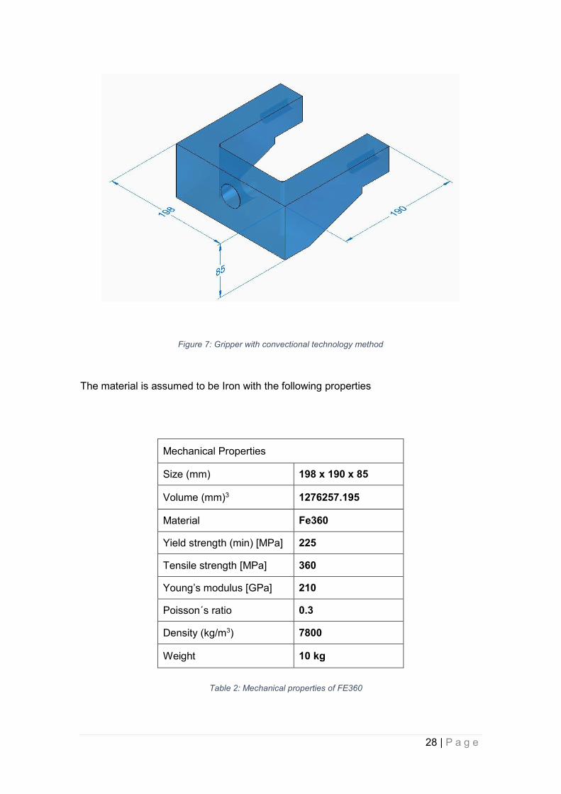
Figure 7: Gripper with convectional technology method

The material is assumed to be Iron with the following properties

Mechanical Properties

Size (mm) 198 x 190 x 85

Volume (mm)3 1276257.195

Material Fe360

Yield strength (min) [MPa] 225

Tensile strength [MPa] 360

Young’s modulus [GPa] 210

Poisson´s ratio 0.3

Density (kg/m3) 7800

Weight 10 kg

Table 2: Mechanical properties of FE360

29 | P a g e

4.1.1. Problem formulation - Loading and boundary: This gripper in one side it fixed with a PIN at the middle

of it to one jaw of SCHUNK gripper and in the other side it holded the product for

handling. The Maximum forces of SCHUNK gripper is 18 kN for both jaws and

obviously 9kN for each jaw. Due to the symmetric shape of evaluated gripper,

the assumed force is 6kN in z-direction. - Objective: The objective is to minimize the mass while keeping the stresses

within safe levels. Safe levels are for simplicity assumed to be 80% of the yield

stress of new material, which in this case is :

𝜎𝑚𝑎𝑥 = 0.8 . 𝜎𝑦

There are also no constraints on the design due to the fact that the component

should be feasible to manufacture in AM.

- FE – Analysis (VON MISES ANALYSIS)

𝜎𝑚 = 58.66 𝑀𝑃𝑎 (a)

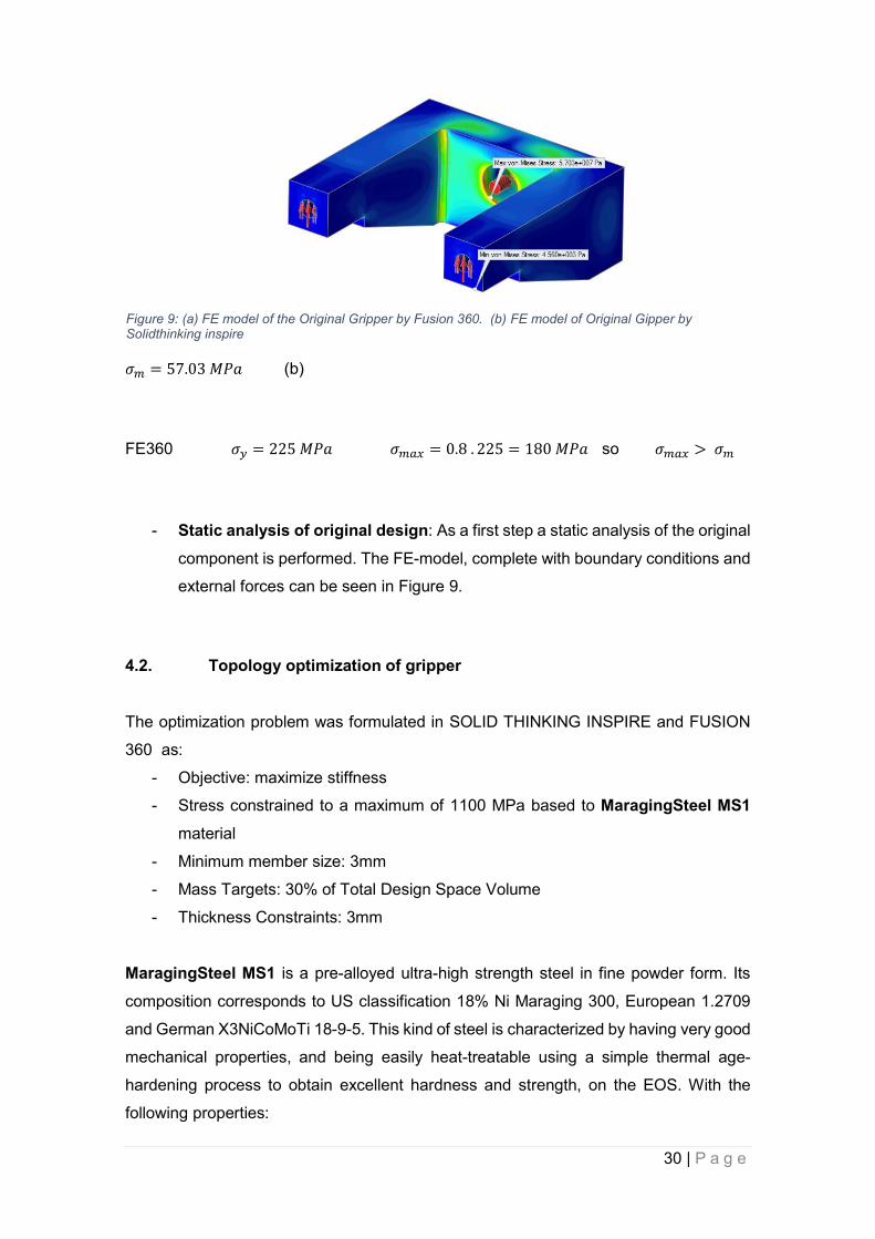
Figure 8: Loading and boundary conditions of Original Gripper

30 | P a g e

𝜎𝑚 = 57.03 𝑀𝑃𝑎 (b)

FE360 𝜎𝑦 = 225 𝑀𝑃𝑎 𝜎𝑚𝑎𝑥 = 0.8 . 225 = 180 𝑀𝑃𝑎 so 𝜎𝑚𝑎𝑥 > 𝜎𝑚

- Static analysis of original design: As a first step a static analysis of the original

component is performed. The FE-model, complete with boundary conditions and

external forces can be seen in Figure 9.

4.2. Topology optimization of gripper The optimization problem was formulated in SOLID THINKING INSPIRE and FUSION

360 as:

- Objective: maximize stiffness

- Stress constrained to a maximum of 1100 MPa based to MaragingSteel MS1 material

- Minimum member size: 3mm

- Mass Targets: 30% of Total Design Space Volume

- Thickness Constraints: 3mm

MaragingSteel MS1 is a pre-alloyed ultra-high strength steel in fine powder form. Its

composition corresponds to US classification 18% Ni Maraging 300, European 1.2709

and German X3NiCoMoTi 18-9-5. This kind of steel is characterized by having very good

mechanical properties, and being easily heat-treatable using a simple thermal age-

hardening process to obtain excellent hardness and strength, on the EOS. With the

following properties:

Figure 9: (a) FE model of the Original Gripper by Fusion 360. (b) FE model of Original Gipper by Solidthinking inspire

31 | P a g e







Thermal conductivity (W/m °C) 15

Specific heat capacity (J/kg °C) 450

Table 3: Mechanical properties of MaragingSteel MS1- As Built







Thermal conductivity (W/m °C) 20

Specific heat capacity (J/kg °C) 450

Table 4: Mechanical properties of MaragingSteel MS1- After age Hardening

32 | P a g e

Figure 10: Results from topology optimization, red areas have high density and white areas

4.2.1. TO method with SOLID THINKING INSPIRE (ALTAIR)

MS1– As Built MS1- After age Hardening Original weight: 10 kg Optimized weight: 3.92 kg

33 | P a g e

Figure 11: Results from topology optimization, red areas have high density and blue areas

4.2.2. TO method by FUSION 360 (AUTODESK) 4.2.2.1. MS1– As Built MS1- After age Hardening

Original weight: 10 kg Optimized weight: 3.02 kg

34 | P a g e

Figure 12: 3D Printed part modeled by Fusion 360

Figure 13: 3D Printed part modeled by Solidthinking Inspire

Figure 14: 3D Printed part with polymer Technologies

35 | P a g e

Figure 15: Mesh file of Optimized model by Fusion 360

Figure 16: Realized model by Solidthinking Inspire PolyNURBS command

4.3. Realization of concept The new modeling method in Solidthinking inspire (PolyNURBS) allows you to trace over

optimized result with Precision, ease and efficiency.

Optimized shapes obtained in Inspire can only be exported in STL format to other CAD

software. STL geometry is represented as triangulated polymeshes, which are great for

concept design and 3D printing, but not directly compatible with subsequent CAD tools

or manufacturing. NURBS are preferred in these use cases because they more

accurately and efficiently represent curved geometry. However, converting third order

meshes to NURBS is often very time-consuming.

At solidThinking, it is addressed this concern by developing a solution called

PolyNURBS. This new modeling method allows you to easily trace over optimized results

to create a smoother, watertight NURBS version of the STL geometry. The resulting

model can be exported to other CAD systems and is readily usable for manufacturing.

The resulting Gripper has a mass of 3.09 kg, which is 30.9% of the mass of original

design.

36 | P a g e

Figure 17: Safety Factor result of realized model

Figure 18: Displacement result of realized model

4.4. Static analysis of realized model A static analysis is performed on the realized model, the Maximum Yield Strength of

Material for MS1 – As Built is 1000 MPa (80% = 800 MPa) and for EMS1 – After Age

Hardening is 1900 MPa (80% = 1520 MPa). In addition, according to Von MISES Stress

analyzing the Maximum stress of realized model must be less than the Max yield strength

of the material then there is no failure in our design.

4.4.1. FEM Analysis of Optimized Gripper

MS1– As Built

37 | P a g e

Figure 19: VON MISES result of realized model

Figure 20: Strain result of realized model

Figure 21: Safety Factor result of realized model

MS1– After age Hardening

38 | P a g e

Figure 22: Displacement result of realized model

Figure 23: Stress VON MISES result of realized model

Figure 24: Strain result of realized model

39 | P a g e

4.4.2. CONCULOSION

- This procedure of optimizing the clip was straightforward and resulted in a design that

was lighter and at the same time fulfilled the requirements.as it mentioned before the

maximum stress with VON MISES method 366.3 MPa (Figure 19,23) that is less than

80% of max Stress Strength of material (800 and 1520 MPa).

MaragingSteel MS1- As Built

𝜎𝑦 = 366 𝑀𝑃𝑎 𝜎𝑚𝑎𝑥 = 0.8 . 1100 = 800 𝑀𝑃𝑎 so 𝜎𝑚𝑎𝑥 > 𝜎𝑚

MaragingSteel MS1- After age Hardening

𝜎𝑦 = 366 𝑀𝑃𝑎 𝜎𝑚𝑎𝑥 = 0.8 . 1900 = 1520 𝑀𝑃𝑎 so 𝜎𝑚𝑎𝑥 > 𝜎𝑚

According to Safety Factor results (Figure 17,21) the Min SF of realized gripper before

hardening treatment is less than 3 and after its treatment is higher than 3. So based to

safety factor definition as bellow:

SF= Material Strength / Actual Stress

It can be derived that this realized model satisfied all requirement of problem definition

with 30 % of mass of the original gripper.

40 | P a g e

4.5. Additive Manufacturing of Optimized Gripper After realizing, the model based to Topology optimization result, as a next step in this thesis the Production method (AM) is discussed. As it can be found in the Chapter 2. There are many Technologies in AM and according to kind of materials (polymers, Metals, Ceramics) the Metal Technology is assumed due to problem definitions and requirements.

Metal technology is divided to several methods as bellow;

SLS™- Selective Laser Sintering;

DMLS™-Direct Metal Laser Sintering;

SLM™- Selective Laser Melting:

EBM™- Electron Beam Melting;

SHS™- Selective Heat Sintering;

MJF™- Multi-Jet Fusion

DMLS technology is defined from other techniques to this thesis according to the following advantages:

Better finish and structures

Bigger size of build envelope

Already established in the automotive industry

Many machine suppliers

Can handle many different material

Slower build process

With this as a background, a benchmark of many of the most well-known DMLS system

suppliers was done to find the most suitable machine for the simulation.

These suppliers are the most famous and established companies in the industry. From

this benchmark, Concept Laser, EOS and SLM solutions were the three best alternatives

for the study parameters above. These three machines are checked in the software

Autodesk Netfabb 2019 [34] which is a software for build simulations. Concept Lasers

machine was not available for software simulations so it was only two solutions left.

These two machines are compared with the same component to check which performed

best in fact of volume and build speed. the simulation of both machines is evaluated and

compared together.

41 | P a g e

Figure 25: Realized Gripper in an EOS M 290

AM System Suppliers

Supplier Model Technology Build Size (X x Y x Z) MM Deposition (cm^3/h)

Laser Power

3D Systems

ProX DMP 320

DMLS 275x275x420 Not available 500W

EOS M 290 M 400 DMLS 250x250x325

400x400x400 100 4x400W

SLM Solution

SLM 500 HL DMLS 500x280x365 105 4x700W

Phenix Systems

PXL System DMLS 250x250x300 Not

available 500W

Renishaw RenAM 500M DMLS 250x250x350 Not

available 500W

Concept Laser

X LINE 2000R DMLS 800x400x500 120 2x1000W

Realizer SLM 300i DMLS 300x300x300 37 1000W

Arcam Arcam A2X EBM 200x200x380 Not

available 8000W

Table 5: AM System suppliers

42 | P a g e

Figure 26: Realized Gripper in an SLM 500 HL – CASE (a)

EOS M 290

Gripper Volume (cm3) 386.35

Support Volume (cm3) 32.78

Build height (mm) 88.08

Build Time (h) 88:43:17 Table 6: Build properties of EOS M 290

SLM 500 HL




Build Time (h) 76:52:22

Table 7: Build properties of SLM 500 HL – CASE (a)

43 | P a g e

Figure 27: Realized Gripper in an SLM 500 HL – CASE (b)

The EOS machine could build Gripper in 88:43 hours and the SLM 500 HL [35] could

print gripper in 76:22 hours. It gives the EOS m 290 a build rate of 12 hours higher than

SLM 500 HL. Therefore, due to build speed and Cost evaluation SLM 500 HL had better

performance so it is selected for all the simulations.

As it can be seen in Figure 25, 26 the gripper is planted on platform of machine while

printing so in the next step it is tried to use change the orientation of printing in order to

reduce time and cost of building.

SLM 500 HL




Build Time (h) 85:52:38 Table 8: Build properties of SLM 500 HL – CASE (b)

44 | P a g e

Figure 28: Realized Gripper in an SLM 500 HL – CASE (c)

According to the Table 7, 8, 9 CASE (a) had the minimum build time about 77 hours.

However, it does not mean that case (a) it is a best orientation of printing of optimized

gripper because it has to consider about post processing operations like leaving

temporary supports which is helped during printing and clearing and creating smoothed

surface and other criteria like this. In the next step it is evaluated the Cost and

Sustainability of this product in order to find the best orientation of 3D printing in AM

technologies and also it is compared the differences between CM and AM as a cost and

sustainability point of view.

SLM 500 HL




Build Time (h) 85:17:13

Table 9: Build properties of SLM 500 HL – CASE (c)

45 | P a g e

4.6. Cost and Sustainability of AM 4.6.1. Manufacturing Cost Analysis AM building cost: According to the pervious chapter result for Additive manufacturing by Autodesk

NETFABB, three possible calculation are evaluated to understand the minimum cost of

realized gripper. As it can be seen in Appendix (A) the Total Cost of building of optimized

gripper with Additive manufacturing method for Case (a) is 3537.3 € for Case (b) is

3509.5 € and for Case (c) is 3734.2 € .

Therefore, Case (a) and (c) had a higher product Price than case (b).

Although in case (a) the building time is less than case (b) but as it mentioned before

based to orientation of product during 3d Printing in order to create less support which

made post processing work it has to be tilted the product.

In following it is compared the Cost of AM and CM method.

CM building cost:

According to the Appendix (B), the Total Cost of building of in CM is about 625 €.

As a brief comparison between to methods, it can be understood that the CM production

method is better according to defined product of this project because of grade of

complexity of my product.

4.6.2. Sustainability Analysis The Eco-indicator values are intended to be applied by designers and product managers

for the assessment of environmental aspects of product systems. The Standard Eco-

indicators are numbers that express the total environmental load of a product or a

process. These indicators are found in the “Eco-indicator 99 Manual for Designers, a

damage oriented method for life cycle impact assessment”, published by Ministry of

Housing, Spatial Planning and the Environment, in Netherlands, in October 2000. The

Eco-indicator methodology conforms well to the ISO 14042 standard on life cycle impact

assessment.

The standard Eco-indicator values are regarded as dimensionless figures. As a name,

the Eco-indicator point (Pt) is used. The unit millipoint (mPt) is used (so 100 mPt = 0.1

Pt). The scale is chosen in such way that a value of 1 Pt is representative for one-

46 | P a g e

thousandth (1 kPt) of the yearly environmental load of one average European inhabitant

[36].

For the purposes of this study, the method of Eco-indicator 99 has been used in order to

estimate the Environmental Impact (EI) of the manufacturing of a Gripper with

conventional technologies (original scenario) and the EI of the same gripper AM using

MS1 and the SLM 500 HL machine. The purpose is to compare the EI of these two

methods.

The Eco-indicators of the production of the components are based to mPts per 1 kg so

the mPts of each process is calculated by multiplying the indicator by the mass of each

material.

The Eco-indicator manual does not contain any indicators for any AM technologies so

the Eco-indictor of the SLM 500 HL machine must be calculated. A study performed at

Loughborough University on the AM250 SLM machine by Renishaw (the study uses the

former name MTT SLM 250 of the same machine) using the Stainless Steel 316L powder

calculates the power consumption of the machine. The study focuses on the electrical

consumption of the machine during the process. The average energy consumed per kg

is calculated to 31 kWh [37]. Moreover, the EI of the SLM 500 HL machine is evaluated

according to the following equation:

𝐸𝐼 = 𝑓𝑐𝑒𝑙𝑒𝑐𝑡𝑟𝑖𝑐𝑖𝑡𝑦 × 𝐸𝐶𝑅

Where ECR is the Energy Consumption Rate or massive energy use during the process

such as :

𝐸𝐶𝑅 =𝑃

𝑃𝑃=

𝑃

𝑞𝑚𝑎𝑡 × 𝜌𝑚𝑎𝑡

In addition (=10 mPts/kWh) is the indicator which allows to convert a massive energy

(ECR) to an environmental impact per kg express in mPts/kg. In the above equation,

represents the electric power consume by the laser during manufacturing (in W),

represents the process productivity (in kg/h), represents the quantity of powder fused

per hour (in cm3/h) and is the density of the material (in kg/cm3) [38]

Consequently, since the ECR is 31 kWh/kg, the EI of the SLM 500 HL machine using

MS1 as a powder material is calculated to 310 mPts/kg. This value is used as the Eco-

indicator of the “SLM 250” process.

The table can now be filled in for each phase in the life cycle and the relevant Eco-indictor

values can be recorded. The score is then calculated for each process and recorded in

47 | P a g e

0

2000

4000

6000

8000

10000

12000

A M C M

TOTAL EI

Use

Processing

Production

the “result” column. The results of the EI of each phase are added and result in the total

EI of the life cycle of the Gripper.

The Table 10 shows the EI (mPts) calculated for every phase of the life cycle of the

turbocharger together with the sum of them compared with the EI. The fully completed

forms of both life cycles of the turbocharger can be found in the Appendix (C) and

Appendix (D).

Table 10 : The EI (in mPts) for each phase for both AM anc CM technologies

The phase of the production of each component has obviously the greatest impact on

the environment. The development of the Gripper with AM technologies by Topology

optimization reduces the EI from 11165.3 mPts to 5485.47 mPts. So based to TO for AM

contributes to about 50.9 %.

It is significant that there are material production processes in the life cycle of the Gripper

that contribute a lot to the total EI of the production phase.

Phase AM CM

Production [mPt] 1194.8 2750

Processing [mPt] 4018.5 8000

Disposal [mPt] -20.22 -148.7

Total [mPt] 5485.47 11165.3

Chart 2: A comparative chart of the EI for the total LC of Gripper

48 | P a g e

A comparative Chart 2 illustrates the EI of the total life cycle of the gripper for both

Technologies and the EI of just the phase of the production of the components of the

turbocharger for both of them.

49 | P a g e

5. Conclusion and Discussion 5.1. Conclusion

Additive Manufacturing (AM) comprises technologies that create objects sequentially

adding layers over each other. The technologies are grouped according to the material

that they use. During the last few years there have been improvements in the metal

technologies along with the metal materials used. Analysis over different technologies

and machines of metal AM has shown that the technologies are not only different in

terms of processes and machines, but also in terms of material, post processing and the

desired accuracy. So one should carefully decide which technology should be chosen

for each product type.

During the recent years the substantial improvements in terms of production cost,

materials properties, part quality and accuracy of technologies, made AM a more

competitive manufacturing way over different industrial applications. Benefited from

flexible and low cost manufacturing solutions, AM production has been applied in several

markets and industries such as Aerospace – Automotive – Customer product – Medical

and … .

An optimized gripper with TO application reduced the mass of product with AM

technology to 30% of original gripper, which was manufactured by CM technology. One

of the development statements of the gripper with AM is the production with the

necessary functional part resulting that uses much less material. The machine chosen

for this development is SLM 500 HL which uses SLM/DMLS technology together with

MaragingSteel MS1 as material input due to its high mechanical properties. It is worth

mentioning that during the research of the metal material properties for the study of AM,

it was unforeseen that parts produced with metal AM technologies have almost the same

or sometimes superior mechanical properties with the conventional manufactured parts.

Many advances have been made in the field of metall materials for the use in AM.

Furthermore, an analysis of the sustainability potential of the development of the critical

component with AM is carried out. The results indicate that the SLM/DMLS technology

has less environmental impact in comparison with CM. However, the analysis is based

only on literature and estimations have been made due to limitations. There is no

available software to use database for the environmental impact of any AM technologies.

Besides these barriers the calculation and the comparison of the environmental impact

of both ways of manufacturing was carried out following the Eco-indicator 99 method.

For AM the impact of the production phase is based on the electrical energy which is

used by the machine and estimations have been made for the impact that occurs due to

the conversion of the metal bulk material to metallic powder. LCA attributed about 87.5

50 | P a g e

% less environmental impact to the use of AM for the production of the gripper. In

addition, the production cost of the aforementioned development has been estimated.

High material and machine prices and low built rates produce expensive products

compared with the conventional manufacturing costs.

5.2. Discussion The sustainability evaluation for new coming technology is necessary and it will help to

provide improvement opportunities for the new product designers. The literature survey

indicates that due to the variety of processing procedures and materials used, there exist

both positive and negative opinions as for the environmental impact of 3D printing, and

it is not easy to draw an exact conclusion. A reasonable conclusion is that the

environmental impact of 3D printing is case-by-case depending on specific situation.

In order to better evaluate the sustainability of 3D printing processes quantitatively and

better guide the decision-makers, this paper proposed a framework for 3D printing

processes sustainability assessment. The integration of product CAD and LCA can

realize the improvement in the early design stage, which is an essential step for 3D

printing.

To realize the sustainable manufacturing is the goal in current industries, it’s unclear

exactly how far we could go with 3D printing or if it will finally be marked as purely

sustainable, but certainly it is a worthy study area now and in the future.

51 | P a g e

52 | P a g e

References

[1] Gibson Gibson, I., Rosen, D., and Stucker, B. (2015). Additive Manufacturing Technologies. [Elektronisk resurs] : 3D Printing, Rapid Prototyping, and Direct Digital Manufacturing. New York, NY : Springer New York : Imprint: Springer, 2015. [2] Christensen, P. W., Gladwell, G. M. L., and Klarbring, A. (2008). An introduction to structural optimization. Solid Mechanics and Its Applications: 153. Dordrecht : Springer Netherlands, 2008.

[3] Clausen, A. (2016). Topology Optimization for Additive Manufacturing. PhD thesis, Technical University of Denmark. [4] Gardan, J. (2016). Additive manufacturing technologies: state of the art and trends. International Journal of Production Research, 54(10):3118 - 3132. [5] Thompson, M. K., Moroni, G., Vaneker, T., Fadel, G., Campbell, R. I., Gibson, I., Bernard, A., Schulz, J., Graf, P., Ahuja, B., and Martina, F. (2016). Design for additive manufacturing: Trends, opportunities, considerations, and constraints. CIRP Annals - Manufacturing Technology, 65(2):737 - 760. [6] Vanek, J., Galicia, J., and Benes, B. (2014). Clever support: E-cient support structure generation for digital fabrication. Computer Graphics Forum, 33(5):117 - 125. [7] Thomas, D. (2010). The development of design rules for selective laser melting. PhD thesis, University of Wales Institute, Cardiff [8] Wang, D., Yang, Y., Yi, Z., and Su, X. (2013). Research on the fabricating quality optimization of the overhanging surface in slm process. The International Journal of Advanced Manufacturing Technology, 65(9):1471 - 1484. [9] Young, Son K. “A Cost Estimation Model for Advanced Manufacturing Systems.”

International Journal of Production Research. 1991. 29(3): 441-452. [10] Reeves P. (2008) “How the Socioeconomic Benefits of Rapid Manufacturing can

Offset Technological Limitations.” RAPID 2008 Conference and Exposition. Lake Buena

Vista, FL: 1-12. [11] Walter, Manfred, Jan Holmstrom and Hannu Yrjola. “Rapid Manufacturing and its Impact on Supply Chain Management.” Logistics Research Network Annual Conference.

September 9-10, 2004. Dublin, Ireland. [12] Neef, Andreas, Klaus Burmeister, Stefan Krempl. 2005. Vom Personal Computer zum Personal Fabricator (From Personal Computer to Personal Fabricator). Hamburg: Murmann Verlag.

[13] University of San Francisco. Walmart: Keys to Successful Supply Chain Management. <http://www.usanfranonline.com/resources/supply-chain-management/walmart-keys-to-successful-supply-chain-management/#.U5IDQfldXzg>

53 | P a g e

[14] Ruffo, Massimiliano, Christopher Tuck, and Richard Hague. 2006. “Empirical

Laser Sintering Time Estimator for Duraform PA.” International Journal of Production

Research 44 (23): 5131–46. [15] Campbell, I., J. Combrinck, D. De Beer, and L. Barnard. 2008. “Stereolithography

Build Time Estimation Based on Volumetric Calculations. Rapid Prototyping Journal. 14(5): 271-279.

[16] Di Angelo, Luca, and Paolo Di Stefano. 2011. “A Neural Network-Based Build Time Estimator for Layer Manufactured Objects.” International Journal of Advanced

Manufacturing Technology 57 (1-4): 215–24. doi:10.1007/s00170-011-3284-8. [17] Hopkinson, Neil, and Phill M. Dickens. “Analysis of Rapid Manufacturing – Using Layer Manufacturing Processes for Production.” Proceedings of the Institution of Mechanical Engineers, Part C : Journal of Mechanical Engineering Science. 2003. 217(C1): 31-39. <https://dspace.lboro.ac.uk/dspace-jspui/handle/2134/3561>

[18] Teece, D.J Pisano, G Shuen, A (1997). Dynamic capabilities of strategic management. Strategic Management Journal, 18(7), pp537-556 [19] EOS. (2013). Industries and Markets. Available: http://www.eos.info/industries_markets. Last accessed 30th May 2014. [20] Mina Aliakbari. (2012). Additive Manufacturing: State-of-the-Art, Capabilities, and Sample Applications with Cost Analysis. KTH Royal Institute of Technology

[21] S.S. Muthu, M.M. Savalani, Handbook of sustainability in additive manufacturing (Publisher Springer Singapore, 2016)

[22] F. Le Bourhis, O. Kerbrat, J. Hascoet, P. Mognol, Int J Adv Manuf Tech 69, 1927– 1939 (2013)

[23] M. P. Bendse and O. Sigmund. Material interpolation schemes in topology optimization. English. Archive of Applied Mechanics 69.9 (1999), 635{654.

[24] Singiresu S. Rao. Engineering Optimization | Theory and Practice. John Wiley & Sons, third edition, 1996.

[25] Matthias Ehrgott. Multicriteria Optimization. Springer Berlin Heidelberg, second edition, 2005.

[26] Carlos A. Coello Coello, Gary B. Lamont, and David A. Van Veldhuizen. Evolutionary Algorithms for Solving Multi-Objective Problems. Genetic and Evolutionary Computation. Springer US, second edition, 2007.

[27] Anders Klarbring and Peter W. Christensen. An Introduction to Structural Optimization. Solid Mechanics and its Applications. Springer Science + Business Media B.V.,2009.

54 | P a g e

[28] G. I. N. Rozvany. Aims, scope, methods, history and unified terminology of computeraided topology optimization in structural mechanics. Struct. Multidisc. Optim., 21:90{ 108, 2000.

[29] G. I. N. Rozvany. A critical review of established methods of structural topology optimization. Struct. Multidisc. Optim., 37:217{237, 2009.

[30] Martin Philip Bendse and O. Sigmund. Material interpolation schemes in topology optimization. Archive of Applied Mechanics, 69:635{654, 1999.

[31] Martin Philip Bendse and Noboru Kikuchi. Generating optimal topologies in structural design using a homogenization method. Computer Methods in Applied Mechanics and Engineering, 71:197{224, 1988.

[32] Solidthinking Inspire 2018.3 - Altair https://solidthinking.com/product/inspire/

[33] Fusion 360 – Autodesk https://www.autodesk.com/products/fusion-360/free-trial [34] Netfabb Premium 2019 – Autodesk https://www.autodesk.com/education/free-software/netfabb-premium [35] SELECTIVE LASER MELTING MACHINE SLM®500 https://slm-solutions.com/products/machines/selective-laser-melting-machine-slmr500 [36] Ministry of Housing, Spatial Planning and the Environment (2000). Eco-Indicator 99 Manual for Designers. Hague. p1-49. [37] M. Baumers, C. Tuck, R. Hague, I. Ashcroft and R. Wildman. (2010). A Comparative Study of Metallic Additive Manufacturing: Power Consumption. Additive Manufacturing Research Group, Wolfson School of Mechanical and Manufacturing Engineering, Loughborough University, p278-288.

[38] Florent Le Bourhisa, Jean-Yves Hascoeta, Olivier Kerbrata, Pascal Mognola. (2013). Sustainable manufacturing: Evaluation and Modeling of environmental impacts in additive manufacturing. The International Journal of Advanced Manufacturing Technology. 1 (12), p1-22.

https://solidthinking.com/product/inspire/

https://www.autodesk.com/products/fusion-360/free-trial

https://www.autodesk.com/education/free-software/netfabb-premium

https://slm-solutions.com/products/machines/selective-laser-melting-machine-slmr500

55 | P a g e

56 | P a g e

Appendix

Appendix (A): Production Building Cost by AM

ADDETIVE MANUFACTRING

CASE (a) CASE (b) CASE (c)

Material MS1 MS1 MS1

Part volume [cm^3] 386.35 386.35 386.35

support volume [cm^3] 32.8 14.35 24.9

Post Procecing volume[cm^3] 7.727 7.727 7.727

(Scale 2:100)

Total post processing 40.527 22.077 32.627

Total volume [cm^3] 426.877 408.427 418.977

Density [kg/m^3] 8000 8000 8000

Total weight [kg] 3.415016 3.267416 3.351816

Material price [€/kg] 120 120 120

Material cost [€] 409.8019 392.0899 402.2179

Building time [hr] 76.5 85.5 85.2

Building price [€/hr] 35 35 35

Building cost [€] 2677.5 2992.5 2982

Post Processing time 9 2.5 7

Post Processing price [€/hr] 50 50 50

Post Processing cost [€] 450 125 350

Product Building cost [€] 3537.302 3509.59 3734.218

57 | P a g e

Appendix (B): Production Building Cost by CM

CONVECTIONAL MANUFACTRING

Material Fe360

Part volume [cm^3] 1276.2

Density [kg/m^3] 7800

Total weight [kg] 9.95436

Material price [€/kg] 2.5

Material cost [€] 25

Building time [hr] 12

Building price [€/hr] 50

Building cost 600

Product Building cost [€] 625

58 | P a g e

Appendix (C): LCI of AM

Addetive Manufacturing

Production of ferro metals (in Millipoints per kg)

Material Amount Unit Indicator Result

MaragingSteel MS1 3.4 kg 86 292.4

mPt 292.4

Processing of ferro metals (in Millipoints per kg)

Process Amount Unit Indicator Result

SLM 500 (50% Solidity) 3.4 kg 310 1054

Post processing 0.176 kg 800 140.8

mPt 1194.8

Use (Electricity )


Electricity LV Ittaly 47 85.5 kWh 47 4018.5

mPt 4018.5

Disposal (disposal processes per type of material)


Incineration Steel (22% in Europe) 0.748 kg -32 -23.936

Landfill steel (78% in Europe) 2.652 kg 1.4 3.7128

mPt -20.2232

Total (all Phases) 5485.477

59 | P a g e

Appendix (D): LCI of CM

Convectional Manufacturing

Production of ferro metals (in Millipoints per kg)

Material or Process Amount Unit Indicator Result

FE360 25 kg 110 2750

mPt 2750

Processing of ferro metals (in Millipoints per kg)


Milling, Turning, Drilling 10 kg 800 8000

mPt 8000

Use (energy)


Electricity LV Ittaly 47 12 kWh 47 564

mPt 564

Disposal (disposal processes per type of material)


Incineration Steel (22% in Europe) 5.5 kg -32 -176

Landfill steel (78% in Europe) 19.5 kg 1.4 27.3

mPt -148.7

Total (all Phases) mPt 11165.3

Date post:	03-May-2020
Category:	Documents
Upload:	others
View:	2 times
Download:	0 times

POLYTECHNIC OF TURINSubsequently, topology optimization (TO) tutorials are studied. These are...

Documents