50
Mixed Integer Conditional Value-at-Risk Portfolio Optimization Multi Disciplinary Approaches M.Sc Defense Ahmed Ashmawy German University in Cairo September 2011

Mixed Integer Conditional Value-at-Risk PortfolioOptimization
Multi Disciplinary Approaches
M.Sc Defense
Ahmed Ashmawy
German University in Cairo
September 2011

Outline
Introduction
Background
Problem Description
System
Hybrid CP/LP Approaches
Greedy Approach
Introduction
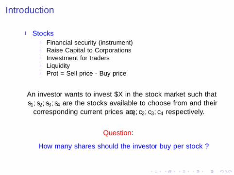
I StocksI Financial security (instrument)I Raise Capital to CorporationsI Investment for tradersI LiquidityI Profit = Sell price - Buy price
An investor wants to invest $X in the stock market such thats1, s2, s3, s4 are the stocks available to choose from and their
corresponding current prices are c1, c2, c3, c4 respectively.
Question:
How many shares should the investor buy per stock ?
Introduction
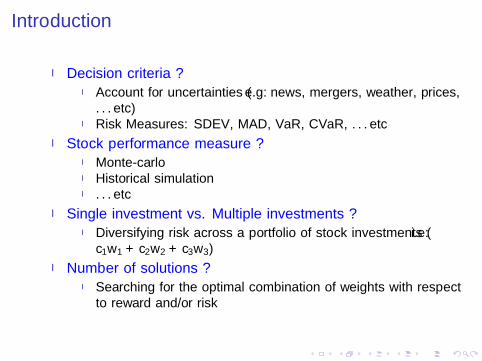
I Decision criteria ?I Account for uncertainties (e.g: news, mergers, weather, prices,
. . . etc)I Risk Measures: SDEV, MAD, VaR, CVaR, . . . etc
I Stock performance measure ?I Monte-carloI Historical simulationI . . . etc
I Single investment vs. Multiple investments ?I Diversifying risk across a portfolio of stock investments (i.e:
c1w1 + c2w2 + c3w3)
I Number of solutions ?I Searching for the optimal combination of weights with respect
to reward and/or risk

Introduction
I Problems- Modeling weight variables as real variables- Hardness of solving mixed integer optimization problems- Gap between Linear & Integer optimization- Mislead investor by inaccurate solutions
I Focus+ Model weight variables as integer variables+ Improving the time performance of the mixed integeroptimization problem

Outline
Introduction
Background
Integer Programming
Value-at-Risk
Conditional Value-at-Risk
Portfolio Optimization
Problem Description
System
Hybrid CP/LP Approaches
Greedy Approach
Integer Programming
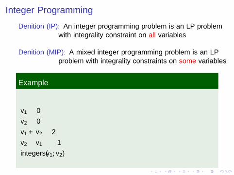
Definition (IP): An integer programming problem is an LP problemwith integrality constraint on all variables
Definition (MIP): A mixed integer programming problem is an LPproblem with integrality constraints on some variables
Example
v1 ≥ 0
v2 ≥ 0
v1 + v2 ≤ 2
v2 − v1 ≥ −1
integers(v1, v2)
Value-at-Risk
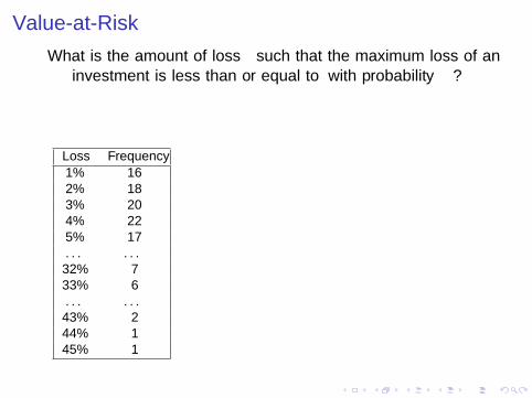
What is the amount of loss ζα such that the maximum loss of aninvestment is less than or equal to ζα with probability α ?
Loss Frequency
1% 162% 183% 204% 225% 17. . . . . .32% 733% 6. . . . . .43% 244% 145% 1
Value-at-Risk
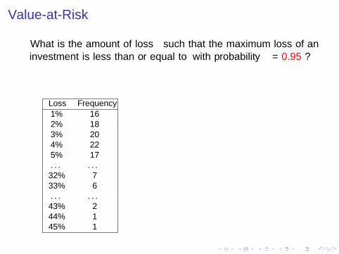
What is the amount of loss ζα such that the maximum loss of aninvestment is less than or equal to ζα with probability α = 0.95 ?
Loss Frequency
1% 162% 183% 204% 225% 17. . . . . .32% 733% 6. . . . . .43% 244% 145% 1

Value-at-Risk
Let f (x, y) be the loss associated with the decision vector x andthe vector y.
The vector x ∈ Rn can be interpreted as the investment portfolioand the vector y ∈ Rm as the uncertainties involved in theportfolio (e.g: prices, weather, . . . etc).
Ψ(x, ζ) =
∫f (x,y)≤ζ
p(y)d(y) (2.1)

Value-at-Risk
Definition (VaR): The Value-at-risk (ζα) is the lowest amount ζwith confidence level α.
ζα = min{ζ ∈ R : Ψ(x, ζ) ≥ α} (2.2)
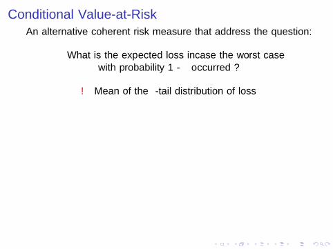
Conditional Value-at-RiskAn alternative coherent risk measure that address the question:
What is the expected loss incase the worst casewith probability 1 - α occurred ?
→ Mean of the α-tail distribution of loss
Conditional Value-at-Risk
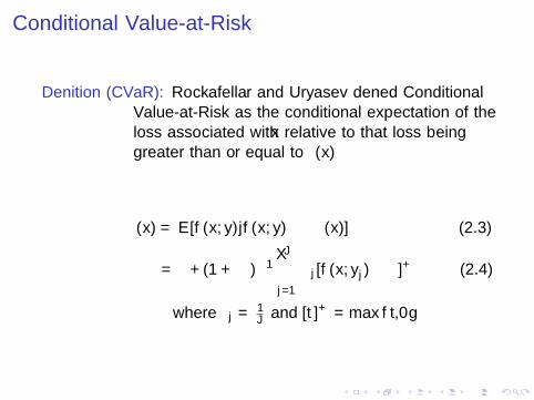
Definition (CVaR): Rockafellar and Uryasev defined ConditionalValue-at-Risk as the conditional expectation of theloss associated with x relative to that loss beinggreater than or equal to ζα(x)
φα(x) = E [f (x, y)|f (x, y) ≥ ζα(x)] (2.3)
= ζ + (1 + α)−1J∑
j=1
πj [f (x, yj)− ζ]+ (2.4)
where πj = 1J and [t]+ = max{t,0}

Conditional Value-at-Risk
I FeaturesI Accounts for risk beyond VaRI Convex functionI Easy to optimize numericallyI Coherent risk measure

Outline
Introduction
Background
Problem Description
System
Hybrid CP/LP Approaches
Greedy Approach
Problem Description
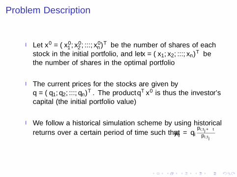
I Let x0 = (x01 , x
02 , ..., x
0n )T be the number of shares of each
stock in the initial portfolio, and let x = (x1, x2, ..., xn)T bethe number of shares in the optimal portfolio
I The current prices for the stocks are given byq = (q1, q2, ..., qn)T . The product qT x0 is thus the investor’scapital (the initial portfolio value)
I We follow a historical simulation scheme by using historical
returns over a certain period of time such that yij = qipi,tj+∆t
pi,tj

Problem Description
f (x, y) = −yTx + qT x0
φα(x) = ζ + (1 + α)−1J∑
j=1
πj [f (x, yj)− ζ]+
where πj = 1J and [t]+ = max{t,0}
I Risk tolerance percentage (ω) is a percentage of the initialportfolio value qT x0 allowed for risk exposure
ζ + (1 + α)−1J∑
j=1
πjzj ≤ ωn∑
k=1
qkx0k (3.1)
zj ≥n∑
i=1
(−yijxi + qix0i )− ζ, zj ≥ 0, j = 1, ..., J (3.2)
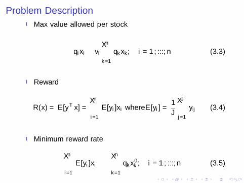
Problem DescriptionI Max value allowed per stock
qixi ≤ vi
n∑k=1
qkxk, i = 1, ..., n (3.3)
I Reward
R(x) = E [yTx] =n∑
i=1
E [yi ]xi where E [yi ] =1
J
J∑j=1
yij (3.4)
I Minimum reward rate
n∑i=1
E [yi ]xi ≥ τn∑
k=1
qkx0k , i = 1, ..., n (3.5)
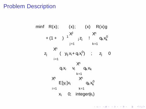
Problem Description
min{−R(x), φα(x), φα(x)− R(x)}
ζ + (1 + α)−1J∑
j=1
πjzj ≤ ωn∑
k=1
qkx0k
zj ≥n∑
i=1
(−yijxi+qix0i )− ζ, zj ≥ 0
qixi ≤ vi
n∑k=1
qkxk
n∑i=1
E [yi ]xi ≥τn∑
k=1
qkx0k
xi ≥ 0, integer(xi)
Outline
Introduction
Background
Problem Description
System
Hybrid CP/LP Approaches
Greedy Approach

System

Outline
Introduction
Background
Problem Description
System
Hybrid CP/LP Approaches
Hybrid Models
Proposed Constraints
Sequential Hybrid Model
Integrated Hybrid Model
Greedy Approach

Hybrid Models
I Hybridization is the process of solving problems using multiplesolvers that co-operate together
I Why use multiple solvers ?I Different solvers/algorithms suit different types of problemsI Solvers complement each other
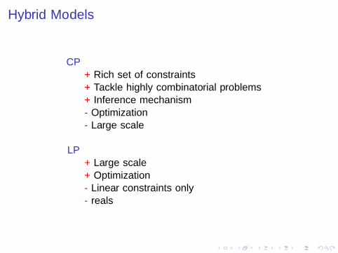
Hybrid Models
CP+ Rich set of constraints+ Tackle highly combinatorial problems+ Inference mechanism- Optimization- Large scale
LP+ Large scale+ Optimization- Linear constraints only- reals

Proposed Constraints
I Shares Constraint
n∑i=1
qixi ≤ Capital (5.1)
I Max Value Constraint
qixi ≤ vi
n∑k=1
qkxk (5.2)
I Min Reward Rate Constraint
n∑i=1
E [yi ]xi ≥ τn∑
k=1
qkx0k (5.3)
Sequential Hybrid Model
I Prune the variable domains using constraint reasoning andthen invoke the external branch & cut solver using the syncedbounds.

Sequential Hybrid Model
Figure: Sequential Hybrid Model Performance, 30 Scenarios
Integrated Hybrid Model
I Branch and Bound algorithmI Co-operating ic and LP solverI Nearest integer first heuristicI Synchronized shared variables

Integrated Hybrid Model
I Slow Convergence
Outline
Introduction
Background
Problem Description
System
Hybrid CP/LP Approaches
Greedy Approach
Greedy Approach: Overview
I MotivationI Complex mixed integer optimization problemI Abandon proof of optimalityI Seek near optimum
I IdeaI Utilize the sparse nature that portfolio optimization problems
exhibit to improve the time performance.
Greedy Approach: Idea
Greedy Approach: Notations
Stock sets I Relaxed stock set: The stock set considered inthe relaxed problem
I Proposed stock set: The stock set extractedfrom the relaxed solution having relaxed weightvalues greater than zero
I Integer stock set: The stock set considered inthe mixed integer problem
Termination Condition is reached if the LP solver fail to contributeto the mixed integer objective function cost (i.e: 2equal subsequent iterations)

Greedy Approach: Algorithm
Algorithm 1
1: L ← U2: I†, W†, R, V ← φ3: C†int , C∗lin ← φ4: repeat5: tmp ← C†int6: L∗, C∗lin ←solveLP(Q, Y, OC|κ,α,ω,υ,ρ, L)7: L ← L \ L∗8: I† ← I† ∪ L∗9: C†int , W†, R, V ← solveMIP(Q, Y, OC|κ,α,ω,υ,ρ, I†)
10: until C†int = tmp or C∗lin = φ

Greedy Approach: Example
Line L I† tmp C†int C∗lin1-4 {1,2,3,4,5,6} φ φ φ φ
6 {1,2,3,4,5,6} φ φ φ 125.32
7 {2,4,5,6} φ φ φ 125.32
8 {2,4,5,6} {1,3} φ φ 125.32
9 {2,4,5,6} {1,3} φ 121.22 125.32
10 {2,4,5,6} {1,3} φ 121.22 125.32
5 {2,4,5,6} {1,3} 121.22 121.22 125.32
6 {2,4,5,6} {1,3} 121.22 121.22 57.32
7 {2,4,6} {1,3} 121.22 121.22 57.32
8 {2,4,6} {1,3,5} 121.22 121.22 57.32
9 {2,4,6} {1,3,5} 121.22 121.22 57.32
10 {2,4,6} {1,3,5} 121.22 121.22 57.32

Greedy Approach: Properties
L∗i ∩ L∗j = φ if i 6= j (6.1)
i⋃k=0
L∗k ⊆ I† (6.2)
C∗lin,i op C∗lin,i+1 (6.3)
C†int,i+1 op C†int,i (6.4)
op =
{≤ if min
≥ if max

Greedy Approach: Experiment Parameters
# Scenarios 30
# Stocks 500, 1000, 2000, 5000, 7000, 9000
# Variables 1000, 2000, 4000, 10000, 14000, 18000
Models IPg , IPbc , IPr
Optimized measure Both
Capital 10,000
Confidence 95%
Risk tolerance 3%
Minimum reward 100%
Maximum value 20%
Period From 2008-01-01 till 2008-07-29
Table: Experiment Parameters

Greedy Approach: Time Performance
Figure: Time Comparison between IPg , IPbc and IPr , Maximizing bothreward and CVaR, 30 Scenarios

Greedy Approach: Share Distribution
Ticker IPbc IPr IPg
0606 360 360 3600990 991 993 991502 4347 4348 43475HT 176 178 1765IH 631 629 631
ADK.W 876 893 875ADL 8895 9103 8906AOM 85830 86986 85809ARW X X 6ARX 5853 5298 5853B08 109 110 109B18 1 X 4CII 91 71 91
CMO 1657 1680 1657E3S 22 25 22
ERNO 11193 1142 11202128W 99 X 71L09 2342 2364 2342
MMZ 2 X X
Table: Share Distribution, 7000 Stocks

Greedy Approach: Solution Quality
Figure: Objective function cost difference between IPg and IPbc ,Maximizing both reward and CVaR, 30 Scenarios
Greedy Approach: Efficient Frontier
Figure: IPbc and IPg Efficient frontiers, 9000 Stocks, 30 Scenarios
Greedy Approach: Efficient Frontier
Figure: IPbc and IPg Efficient frontiers, time performance, 9000 Stocks,30 Scenarios

Conclusion
I Hybrid CP/LP ApproachI Proposing constraints that successfully pruned the search
space of the portfolio optimization problemI Researching the use of hybrid CP/LP models in improving the
time performance of the problem
I Greedy ApproachI Designing a greedy algorithm which exploit the sparse nature
of portfolio optimization problems with focus on improving thetime performance
I Saving 9.86 hours using our proposed greedy algorithm over 15problem instances with respect to solution quality
I Experimental StudiesI Performing experimental studies on real data sets

Thank you

Constraint Programming
I Model the problem as a constraint satisfaction problemincluding variables, their domains and constraints
I Solve using constraint solvers
I FeaturesI Generally known as an efficient inference mechanismI Adequate for solving a wide range of hard combinatorial
problemsI Elegant design framework for developers by separating problem
modeling and solving

Linear Programming
min/max cTx s.t. Ax ≤ b
A =
a1,1 · · · a1,n...
. . ....
an,1 · · · an,n
Example
max 4x1 + 7x2 + 2x3
12x1 − 3x2 + 5x3 ≤ 24
6x1 + 8x2 + 11x3 ≤ 7

Simplex
max 5v1 + 7v2
v1 ≥ 0, v2 ≥ 0
v1 ≤ 1, v1 + v2 ≤ 2

Integer Programming
Definition (IP): An integer programming problem is an LP problemwith integrality constraint on all variables
Definition (MIP): A mixed integer programming problem is an LPproblem with integrality constraints on some variables
Example
v1 ≥ 0
v2 ≥ 0
v1 + v2 ≤ 2
v2 − v1 ≥ −1
integers(v1, v2)
Branch and Bound (B&B)

Branch and Cut (B&C)
I B&C → B&B + Cutting plane algorithm
I Cutting Planes are linear inequalities derived from theconstraint set to remove infeasible linear regions
Example
v1 ≥ 0
v2 ≥ 0
v1 + v2 ≤ 2
v2 − v1 ≥ −1
→ v1 ≤ 1


