5 United States Department,of Agriculture SEP.T. Progress Toward E iminating Hunger in America William T. Boehm Paul E. Nelson Kathryn A. Longen U S -DEPARTMENT-OF HEALTH. EDUCATION WELFARE NATIONAL INSTITUTE OF EDUCATION DOCuME AAS BEEN PEDRO- DuCED EXACTLY AS RECEIVED FROM THE PERSON OR ORGANI-ZATIONCIR ATING IT pOiNTS9F VIEW OR OPINIONS STATED DO NOT NECESSARILY REPRE- S-ENT_OFFICIAL NATIONAL LNSTLT_uTE OF EOUCATION POSITION OR POLICY Economics, Statistics, and Cooperatives Service 0- Agricultural Economic Report No.446
Transcript
5 United StatesDepartment,ofAgriculture
SEP.T.
Progress Toward E iminatingHunger in AmericaWilliam T. BoehmPaul E. NelsonKathryn A. Longen
U S -DEPARTMENT-OF HEALTH.EDUCATION WELFARENATIONAL INSTITUTE OF
EDUCATION
DOCuME AAS BEEN PEDRO-DuCED EXACTLY AS RECEIVED FROMTHE PERSON OR ORGANI-ZATIONCIRATING IT pOiNTS9F VIEW OR OPINIONSSTATED DO NOT NECESSARILY REPRE-S-ENT_OFFICIAL NATIONAL LNSTLT_uTE OFEOUCATION POSITION OR POLICY
Economics, Statistics,and CooperativesService
0-
AgriculturalEconomicReport No.446
PROGRESS TOWARD_ ELIMINATING HUNGER IN AMERICA; By William T. Boehm, Faul E. Nelson;and Kathryn A. Longen; National Econotics Division; Economics, Statistics; andCooperatives Service; U.S. Department of Agriculture. Agricultural Economic ReportNo. 446.
SUMMARY
ABSTRACT
Food assistance funds in the United States have generally gone to areas mostin need. Assistance in the-most needy- U.S. counties averaged-$21.98 perperson it_1967; By 1976; it had increased to:$153.91._ Corresponding figuresfor the least needy counties were $2.04 in 1967 and $26.35 in 1976. Foodassistance payments_ accounted for almost 18 percent of each real dollarincrease in per capita retail food saIes in the neediest counties; Additionalfood spending was influenced more by increases in food assistance paymentsthan by increases in earned income.
Progress has been made-in providing-food for -poor people in ale United States;Persons residing in counties with the highest rates of infant mortality_received_anaverage of_$123.33 in Federal food assistance during 1976, up from $12.83 in 1967. Ili
the Nation's lowest income counties the assistance rose from $21.98 to $153.91;
County groups with the lowest infant mortality rates in_1967_received foodassistance of $2.04 per person in 1967-and-$30.96 in 1976. The highest incomecounties received $2.04 and $26.35; respectively.
Retail food-sales per person reflected -the- availability of food assistancedollars; The increase in real per capita_retail food sales over the decade:(1967-76)was -most obvious for counties with the highest infant-mortality rates. Foodassistance in the form -of bonus- stamps- accounted- for -15.8 cents of each dollarincrease in these sales; In the lowest income counties; the_corresponding_fignre was10.0 cents. In the other county categoriesit the impact was less pronounced. However,with but one exception, it was positive and statistically significant;
Food- assistance distributed-through the National School Lunch and Commodity-Distribution Programs -did- not, -with one exception, result in observable increases inretail food sales. Most food purchased under these two programs comes:fromwholesalers and food manufacturers. :In the poorest rural counties, dollars which theU.S. Department of- Agriculture transferred to schools for school lunches generatedslight increases in retail food sales.
ii
Progress Toward Eliminating Hunger in America
William Boehm; Paul E Nelson; Kathryn A. Longen
INTRODUCTION
Our purpose in this-report-is to.assess the-impact of food assistance programs onhunger in-- America. An earlier study, published in 1968 by the Citizens Board ofInquiry into Hunger and Malnutrition in the United States (CBHM),_documented theexistence of hunger in America. In the current study, we assess the issue indirectlyby treating two questions:
* Have counties-where-hunger was-greatest in 1968 received relatively more foodassistance per person since that time?
* To what extent have food assistance payments been reflected in per capitaretail food sales in these counties':
Before answering these-questions, we define hunger and identify groups ofcounties characterized as being the most in need and the least in need of Federal fa-cidassistance. We -trace the development of domestic food assistance programs since 1968;and we assess the extent of their success.
The earlier CBHM study - -Hunger U.S.A. had reported the following findings:
* One-fifth of U;S; households had "poor" diets as determined by the U.S.Department of Agriculture (USDA).
* Thirty-six percent of low-income households subsisted on "poor" diets.
*- People in 266-U.S. counties-were living in such distressed conditions "as_to_ _warrant a Presidential declaration naming them as hunger areas" (1, p. 85). 1/
The current study was prepared in-response to an inquiry from the White HouseStaff who wanted to know where food assistance dollars went from 1968 -(the date of theCHM study, Hunger.U.S.A.) to 1976 (nearly a decade later). We have focused -on- -those
county groups identified-by CBHM. Our tabulations were based on the most recentcounty.-level records available, those compiled by USDA's'Food and Nutrition Servize(FNS) in 1976. Our study shows that Federal food assistance funds have generally goneto those areas most in need.
I/ Underscored numbers in parentheses refer to references listed at the end of thisreport;
HUNGER IN PERSPECTIVE
Hunger has been defined as a craving for food; a weakened condition brought aboutby prolonged lack of food, and an urgent need for food. Regardless of the definition;hunger is clearly a-condition of degree. That is, the continuum describing hungerruns from a temporary (even self-imposed) discomfort to death.
The CBHM defined hunger as "a condition where people are forced-to-go days eachmonth without one full meal;" Although this definition contains some nonmeasurableand ambiguous elements ("forced," "full meal," and "days each month"), it does ingeneral lend itself to measurement.
Furthermore, the CBHM definition embodies the element of force an&the_concept ofdegree. Self-iMposed hunger, a refusal to eat when food is available, is likely to beviewed differently from hunger which exists because food is not available forconsumption.
Data on Hunger
The only nationwide data relating to food consumption collected by the U.S;Government sincethepublication of Hunger U.S.A.:are those:of the U.S. Department ofLabor's Bureau of Labor Statistics. These data, known as the Consumer Expenditure-Survey (CES), reported food expenditures for about 12;000 households during 1973 and1974 _(18). Unfortunatelyi because of the need to protect the identity of reportinghouseholds, identifying the location of residence (except -for the-Census region) isimpossible; Furthermore, these data record only expenditures on food and some nonfooditems made during a 1-week period._ They_provide no- information on either frequency ofpurchase or the consumption of food obtained through nonmarket sources for example,gardens);
Data are being-tabulated from the 1977-78 Nationwide Food_Consumption Study(NFCS) of USDA's Agricultural Research Service (now part of the Science and EducationAdministration). 1When_they become available in 1980-81_, they will -1--e the mostcomprehensive nationwide source on- food -consumption. These NFCS data (which arecomputed in pounds and ounces of food consumed) will be used to help define theincidence of hunger in the population at large.
The authors of Hunger U.S.A. relied heavily on the corresponding 1965-66Household Food Consumption Survey to document the existence of poor diets in America(4). Those data showed, for example, that just over 50 percent of the low-incomehouseholds in the United States had "good" diets; that is, they met the RecommendedDietary Allowance (RDA) for seven nutrients (16). From the available data, USDAanalysts could not determine whether the diets of the poor had deteriorated more thanthose of higher income groups.
-Several other data-sources provide information on a-ggregate=indicatOrs- of bothpoverty and hunger, by county; However, such data cannot bq relied upon to define theexistence_of hunger very precisely; primarily because they provide no measure of totalfood intake and are available only annually. They are of little use in identifyingthe extent of the hunger problem as they mask the frequency with which it occurs.
Indicators of Hunger
StudieS-, like the ones conducted by CBHM, provide useful information bydocumenting the existence of hunger. But they cannot be relied upon to quantify its
severity. One can, hiowever,, monitor potContribute to its occurrence._ Three oflack of resources to make foOd purchasesoutlets or production resources; and (3)and/or selection of food.
Lack of Resources
ential hunger by monitoring those factors thatthese factors have long been recognized:- (1)
, (2) lack-of access to food distributionlack of knowledge regarding availability
The American food system is market oriented. That is, the available foods (like
other goods and services) are rationed in_thamarketplace to those with the resources
to purchase them; In one sense, ltiis very much like barter7-people trade their
dollars for food. Those without dollars are inlaipoor-position to trade; However, as
food_is necessary to survival;- available resources tend to be allocated to_food,
purchases firstalthough not sufficiently to provide an_adequate diet. ThUa-,-data
indicating the proportion of total income_spent on food by income class help measure
the extent of potential hunger domestically.
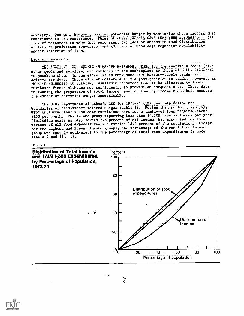
The U.S. Department of Labibr'a CES fibt 1973 -74 (19)icanhelp define the
boundarieS of thia-intOte-related_hunger (table 1). During that period (1973-74),USDA estimated that a low-cost nutritious diet fora familTiof fOur,reqUirad-AbOUt
$150 per month. The income group reporting less than $4,000 pre -tax income per year
(including Mea16-68 pay) earned 6.5 percent of all income; but'accounted_for 15.4
percent of aIl_food expenditures and totaled 18.2 percent of_the population, Except
for the highest:and lowest income groups, the percentage of the population in each
group was roughly equivalent to the percentage of total food expenditures it made
(table 2 and fig. 1),
Figure 1
Distribution of Total Income Percentand Total Food Expenditures, 100
by Percentage of Population,1973.74
80
60
40
2
Distribution of food-expenditures
Distribution ofincome
20 40 60 80 100
Percentage of population
Table 1--Relationship between income and expenditures for food, 1973-74 -/
: Food expenditures: . :
Total Total : Food as aIncome Total . as a ratio of
reported : food percentageclass : population : : Thrifty Food Planincome incomeexpenditures of inco
cost 2/
Less than
Percent Ratio
$4,000 18.19 6.47 15.39 38.88 1;09
$4,000 to$7;999 14.14 9.31 13.09 23.01 1;19
$8,000 to$11,999 21.17 17.79 20.35 18.72 1;23
$12,000 to$14,999 : 14.47 14.65 14.08 15.75 1;26
$15,000 to$20,000 16.07 19.86 17.29 14.26 1;39
More than$20;000 : 15.96 31.92 19.80 10.17 1;60
Total 100.00 100.00 100.00
= -Total is not applicable.1/ Data from 1973-74 Consumer Expenditure Survey, Bureau of Labor Statistics.2/ Adjusted for a family of four (1.00 = $150 per month);
Table 2--Relationship between income and food_expenditures; cumulative totals;1973-74 1/
Annualincome
: Total Total reportedincome
: Total food: expenditures-PoPulation
Percent
Less than $4;000 18;19 6.47 15.39
Less than $8,000 : 32.33 15.78 28.48
Less than $12,000 53.50 33.57 48.83
Less than $15,000 67.97 48.22 62.91
Less than $20,000 : 84.04 68.08 80.20
All classes 100.00 100.00 100.00
1/ Data from 1973-74 Consumer Expenditure Survey Bureau of Labor Statistics.
Weekly fObd-expenditures per person totaled $10.24 in the lowest income group and$15.02 in the highest income group; Households in tbe_lowest income_group_spentalmost 40 percent of tbeirpre-tax income on food. Unfortunately,these 1973-74 CESdata- are too old to reflect any increases in food-buying resource availability forlow- income consumers that may have occurred sit.ce the expansion of the Food StampProgram in 1974.
Lack of Access
Even if purchasing resources are available; consumers must have access to food.:Lack of access is a potentially serious problem for those living in remote areas suchas on_Indian reservations or in the Appalachian Mountains. Lack of access may also bea problem in the ghettos of our industrial cities; among the elderly; and among somechildren.
Data from the 1972 Census of Retail Trade show that half of all_U.Scities hadabsolute declines in grocery store sales area (store spaceZ during 1972 (13).Supermarket sales capacity increased in about 85- percent- of-the surburban areas ascompared with 65 percent of the cities; Such data; although not sufficient to_indicate that food availability is a problem; suggest it may be a greater problem inurban areas where high concentrations of poor people reside.
Other data; however; indicate thar_signifiz.ant quantities of nonmarket food areconsumed by some persons. In a recent USDA survey, -44 percent-of all householdsinditatd-that; during 1976; they had a home fruit or vegetable garden (3). Thirty-one percent reported having a garden formore than ll_years. Per capita consumptionof processed:fruits and vegetables from home gardens has been estimated at about 12percent of all processed fruits and vegetables for 1976 (3). In addition; it islikely that among some groups of_low-income people and in some rural_areas significantquantities of meat and dairy products are produced for home consumption and are;therefore, not reflected in aggregate food purchase data;
Lack of Knowledge
Individual choice plays a substantial role_in determining what_people eat in theUnited States. The food-selection and-consumption proc:,:ses are related in a rathercomplicated fashion to other aspects of life. For example,:the_per_capita consumptionofAairy products:among black Americans may be low because blacks often,havedifficulty digesting-lactose. -Teenage school children may choose not to participatein the National School Lunch Program to spend theiv hour_away from_school. Such
personal decisions influence nutritional status an contribute to malnuttittoti in
America.
Educational level has beenLidentified 4s one of the most importantfactOtSinfluencing fbod Chdide. Data from both the 1955 and 1965 Household Food ConsumptionSurveys indicate that; on average; the highly educated homemaker- spends more_for foodper person:in the household_(15)._ This individual tends to purchase more milki_fruits, and vegetables and less flour and fewer cereals, dry beans, and peas. But
even when income is excluded as a variable; education is a factor in food selection.After a thorough analysis of the data, one researcher concluded:
Regardless of the amount of money spent per person for food, among householdswith less education, there_was_a larger proportion with poor diets. AmOnghousehold§ earning under $3,000 the percent of poor diets increased as educationdecreased (8).
9
DOMESTIC FOOD PROGRAMS
Hunger indicators have been_used extensively in the development of_publicprograms to eliminate or reduce the severity of hunger in America, -Such indicatorsprovide_a convenientimechanism for:identifying target groups; Typically; eligibilityfor fbod-assistance is related to income. Only in rare instances has hungerLitselfbeen considered a sufficient condition for participation in public domestic foodassistance programs. When it has; the program has -often been viewed as temporary andemergency relief (usually resulting from a national disaster).
USDA has_operated food_assietance programs since 1935. Emergency fooddistribution-during-the-early thirties expanded into a family of relate&programsaimed at improving the nutritional status of infants; children, and- -low- income -
families. Until recently; such programs were operated largely as mechanisms forsurplus removal,-designed primarily to help support farm income. _Events of the latesixties; including publication of Hunger U;S;A,, began to change that-Oblicyperception. Today; while the food programs continue to contribute to the support offarm income,-they are more generally regarded as programs of income assistance t1-atimprove the diets of poor families and children;
Domestic-food assistance has expanded greatly since 1967.- Hunger U.S.A. reportedthat food programs in that year reached "18 percent of the 29,900,000-poor"-(5.4million) (1).L In:first_quarter 1979i more than 18 million persons each monthparticipated in-the Food Stamp Program alone. Participation exceeded 19 million permonth when unemployment was at 7.5 percent in early 1976 (T). Total Federalexpenditures for all food programs increased from $1,063 million in FY 1969 to $7;825million in FY 1976 (table 3).
Programs now in operation include basic commodity distribution; child feedingprograms; a national food stamp program for households; a food program for pregnantand lactating women; infants, and children; feeding programs for the elderly; and anarray of nutrition education programs designed to help low-income shoppers andchildren improve their ability to select and use nutritious foods.
V-6bdS-tainpPrb-gram
TheiFood_Stamp Act of 1964 established_theiFood Stamp Program asia part ofpermanent legislation.- The program was-designed-to correct deficiencies in commoditydistribution programs by permitting households to purchase food through regular marketchannels. Under the act; eligible households were required to -pay about 20 percent oftheir money income to- receive- stamps worth enough to purchasefoods considerednecessary for a low-cost nutritious diet; However; as a result of changes adopted inthe Food and Agriculture Act of 1977, eligible households are no- longer required tocommit cash resources fOr food to participate in the Food Stamp Program.
In its early years, the Food Stamp Program encountered some resistance frompotential participants. Poor people often indicated a preference for direct commoditydistribution; Hunger U.S.A. reported: "In areas where the Commodity- DistributionProgram was being scrapped in favor of food stamps; the low-income family found itselfwhipsawed between a-progrem that had distributed food free and a new program thatassumed that the 'family had paid for itn tood;" (1, p; 59);
Legislative- and administrative changes in the rules and the passage of time_appear to have reduced this early resistance. About 18;4 million persons participatedin the Food Stamp Program in the first quarter of 1979, according to preliminary Foodand Nutrition Service (FNS) figures.
610
Table 3--Federal expenditures for USDA food and nutrition programs, fiscal years 1961-17
2/ Special supplemental Food Program for_Women, Infants; and Children (WIC) was started in Jan, 1974.
3/ Excludes food stamps paid for by participants.
Source: Food and Nutrition Service records;
1112
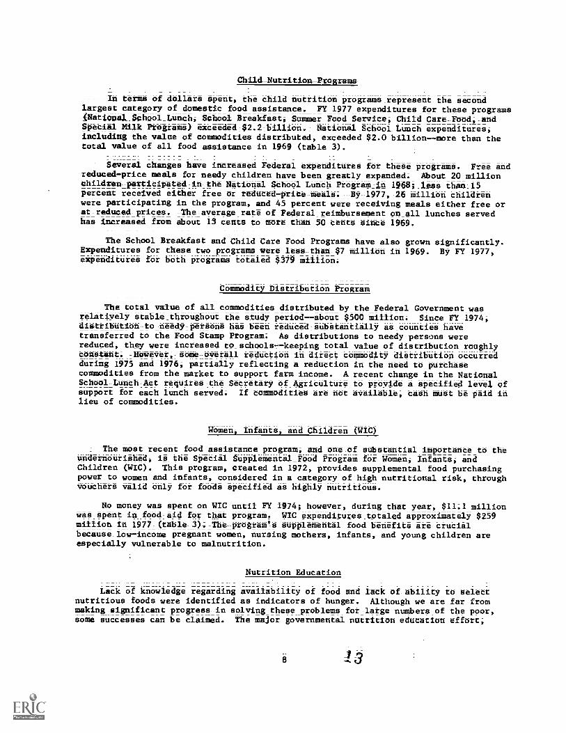
In terms-of dollars spent, the child nutrition programs_ represent the secondlargest category of domestic_food_assistance. FY 1977 expenditures for these programs(National_ School_ Lunch; School Breakfast, Summer Food Service; Child Care-Food, -andSpecial Milk Programs) exceeded $2.2ibillion.i National_School_Lunch expenditures;including the value of commodities distributed, exceeded $2.0 billion- -more than thetotal value of all food assistance in 1969 (table 3);
Several changes have increased Federal expenditures for these programs. Free andreduced-price:meals_for needy:children have been greatly expanded; About 20 millionChildren-participated-in the National School Lunch Program-in 1968; -less than-l5percent received either free or reduced- price meals. -By-1977,-26 million childrenwere participating in the program; and -45 percent were receiving meals either free orat- reduced- prices. -The-average rate of Federal reimbursement on all lunches servedhas increased from about 13 cents to more than 50 cents since 1969.
The- School- Breakfast and Child Care Food Programs have also grown significantly.Expenditures for these two programs were less -than $7 million in 1969. By FY 1977,expenditures for both programs totaled $379 million;
Commodity Distribution Program
The total value of all commodities distributed-by the-Federal Government wasrelatively stable_ throughout the study period--about $500 million; Since FY 1974;distribution-to needy-persons has been reduced substantially as- counties -havetransferred to the Food Stamp Program; As distributions-to-needy-persons were-reduced; they were increased to_schools-keeping total value of distribution roughlyconstant. -However, some-overall reduction in direct commodity distribution occurredduring 1975 and 1976, partially reflecting a reduction in -the need to purchase-commodities -from the market_ to_support farm income; A recent change in the NationalSchool-Lunch-Act requires the Secretary of Agriculture to provide a specified level ofsupport for each lunch served; If commodities are not available, cash must be paid inlieu of commodities.
Women; Infants; and Children (WIC)
The most recent food assistance program; and one of substantial importance to theundernourished* is the Special Supplemental Food Program for Women; Infants; andChildren (WIC);_ This program,-created in 1972, provides supplemental food purchasingpower to women and infants; considered in a category of high nutritional risk; throughvouchers valid only for foods specified as highly nutritious.
No money was spent on WIC until FY 1974; however; during that year, $11;1 millionwas spent in food-aid for that program. WIC expenditures_ totaled approximately $259million in 1977_(table 3)-; The program's supplemental food benefits are crucialbecause-low- income pregnant women; nursing mothers, infants, and young children areespecially vulnerable to malnutrition.
Nutrition Education
Lack of knowledge regarding availability of food and lack of ability to selectnutritious foods were identified as- indicators of_hunger. :Although we are far frommaking significant progress-in solving these problems for large numbers of the poor,some successes can be claimed; The major governmental nutrition education effort,
USDA's Expanded Food and Nutrition Education Program, represents a program which, like.many others discussed here, was established in 1968. However, it was not implementeduntil 1969._ The program operates on a onetoone basis, concentrating on improvingthe-food selection and preparation practices of -low income homemakers. It has beenrelatively successful. However, because of limited resources, the program has beenable to reach only about 20 percent of its target population (17).
HAVE WE MADE PROGRESS?
The number-of food assistance programs and the Federal dollars spent haveincreased dramatically since--1968- stable _3). Even_so,_the persistent questionremains: Has progress been made in our effort to eliminate hunger in America?
Given the earlier definition, hunger can only-be eliminated if the quantity of-food consumed by chronically hungry people is increased on a regular basis. While thefood assistance programs- use indicators of hunger to determine eligibilityi theyoperate on the premise that if food is available, hunger will be eliminated.Obviously; food assistance programs will not be effective unless public funds arechanneled to those areas where hungry people are concentrated.
To determine whether or:not these programs have helped -to- reduce hunger in:Atericao one first needs to know where the hungry people are (figs. 2 and 3). Second,the flow of food assistance dollars must be traced to ascertain whether the dollarsare -going to -those most in need. Third, if- program dollars are going to those most inneed, have they influenced per capita expenditures on food?
Hunger U.S.A. identified six groups of U.S. counties to determine therelationships-among-hunger,-income, and-postneonatal mortality (or death fromthe 2ndto the 12th month after birth); which is a major indicator of infant malnutrition;The county groups were defined as follows:
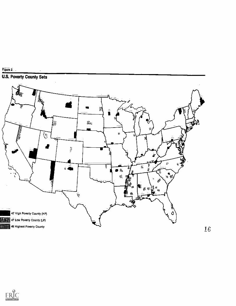
(1) Highest Postneonatal Mortality Counties (HMR): The county in each of the 47States for which postneonatal data were available having the highestpostneonatal-mortality-rate.- -(Data were not published in forAlaska; Hawaii; and New Hampshire.)
(2) Highest Poverty-Counties-(HP): The county in each of-these-States having thehighest proportion of households below the poverty income line;
(3) Lowest Postneonatal MOrtality-Counties-(LMR): -The county-in-each of the 47States for which data were available having the lowest postneonatal mortalityrate
(4) Lowest Poverty Counties (LP): The county in each of these same States havingthe lowest proportion of households below the poverty line.
(5) Highest Postneonatal Counties in the United States (NHMR): The 49 countieswith the highest postneonatal mortality rates nationwide. 2/ More than onecounty per State could be included.
2/ At the outset of the study, 50 counties were chosen.- However, food. assistancedata for two counties were_not reported separately, thereby necessitating combiningall data for the two counties.
Role 2_
U.S Poverty County Sets
47 High Poverty County (HP)
47 Low Poverty County (LP)
49 Highest Poverty County16
Figure 3
U.S. Postneonatal Mortality County Sets
counties with highest postneonatal modality rates (10411,)
Counties with lowest postneonatal mortality rates OAR)
49 highest hunger county
18
(6) Highest Poverty Counties in the United States (NEP): The 49 counties withthe highest proportion of households below the poverty income linenationwide. More than one county per State could be included (see appendix);
Admitting atitheioutset the very close association between income andMalnutrition, CBHM made extensive use of postneonatal mortality rates (MR)_to identifyits hunger counties. Although the -MR does not necessarily reflect the food buyingpotential of people in a county; it was argued that overall the MR was a goodindicator of the existence of hunger. The authors of Hunger U.S.A. state:
The correlation between malnutrition and poverty is reflected in postneonatalmortality_rates. _During the first month of life--the neonatal state--povertyinfants die at only-a-slightly-higher rate than infants from higher incomegroups. From the second to the 12th month; a startling disparity occurs betweendifferent income groups. The rate of death for the_infant from an affluentfamily-drops to approximately one-third theneonatal (first month) rate. Thedeath rate for the poor infant may drop--but nowhere near as radically; and inthe poorest_counties; the postneonatal rate will actually rise appreciably abovethe neonatal rate tl, p. 33).
These sixcounty sets were adopted to_determine whether or_not food assistancepayments_have been flowing to localities-where demonstrated need is greatest. Thehypothesis is that the largest per capita payments will flow to the NHMR and NHPcounties. conversely; the smallest_per capita payments will flow to the LMR and LPcounties. _Furthermore, it-is hypothesized that food assistance payments per personwill be higher for the Nation's 49 NHMR and NHP counties than for the HMR or HPcounties. In_ turn,_ payments received by the_HMR or HP county sets will be larger thanthose received by-either the LMR or LP-counties.- Thus, it is anticipated the percapita_payments received by persons residing in the }U and HP counties will be largerthan those received by people living in the LMR and LP counties.
One obtains per capita payments by dividing the total food assistance paymentsreceived annually within each county by the county's total population. 3/ Thus; theaverage per capita payments to the LMR and LP counties were-lower than the amount thatwould have resulted if only the number of participants throughout the year (adjustedto avoididouble:counting of persons participating in more than one program)lhad beenused as the divisor; For the HMR and HP categories,-using this procedure did notlower the average per capita payments as much because a much higher proportion of thepopulation in these counties received food assistance.
Although the differences among the HMR and HP and the LMR and LP county sets aregreater when the total county population is used_as the divisor, comparisons willindicate whether the direction of fund flow has been in favor of or at the eXpehse ofthe neediest localities.
Average Per Capita Payments
Data in table 4 are consistent with these hypotheses. The payments received bypersons in greatest need--those residing in county_ categories NIINR and NHP--weregreater than those received by persons living in the other county groups. Payments
3/- The mean population of category HMR for the 1967-76 period was 23,741. For theHP counties, it was 33;836. In contrast, the corresponding average for LMR countieswas 78,655; and for LP counties, 290,662. For the NHMR, the mean population was14;461; and for the NHP counties, 13,633.
12
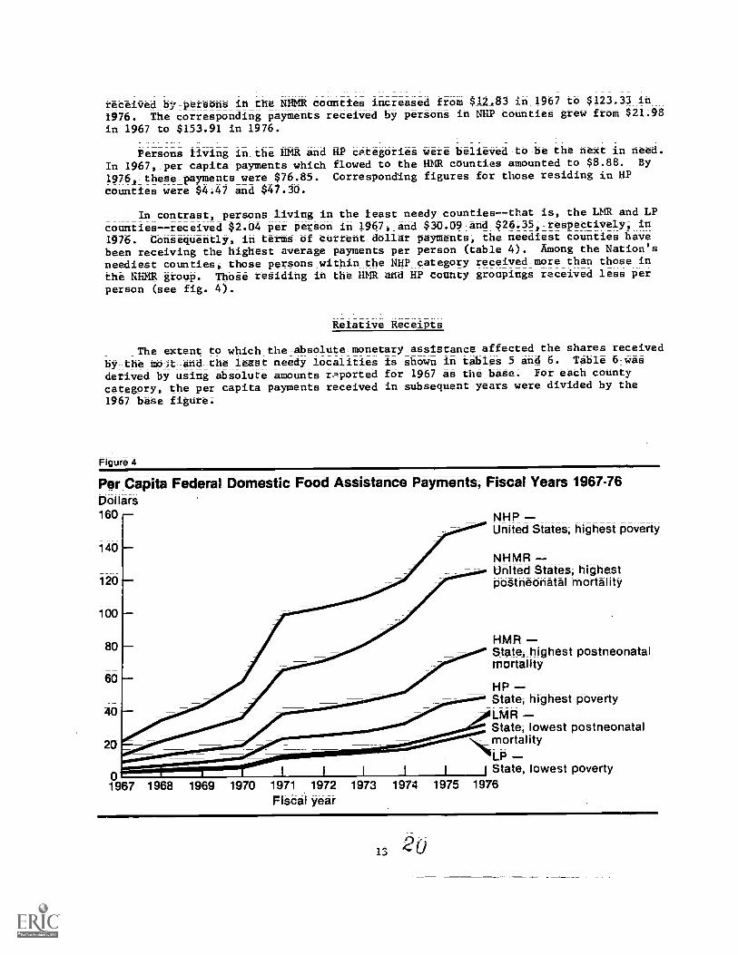
received by-persons in the NHMR counties increased from $12.83 in 1967 to $123.33 in
1976; The corresponding payments received by persons in NHP counties grew from $21.98
in 1967 to $153.91 in 1976.
Persons living in the IIMR and HP cptegories were believed -tb -be the next in need.In 1967j.per capita payments WhiCh flowed to the HMR counties amounted to $8.88. By
1976, these-payments were $76.85. Corresponding figures for those residing in HP
counties were $4.47 and $47.30.
In contrast; persons living in the least needy_counties7that is, the LMR and LP
counties -- received $2.04 per person in 1967,_and $30.09iand $26,35,-respectively, in1976. Consequently, in terms of current dollar payments, the neediest counties havebeen receiving the highest average payments per person (table_4). Among the Natiat'Sneediest countiesj_ those persons_ within__ the NHP category received more than those in
the NHMR group. Th666 residing in the HNR and HP county groupings received less perperson (see fig. 4);
Relative Receipts
The extent to Which the abSolute monetary assistance affected the shares received
by --the MUItt-and the least needy localities is shown in tables 5 and 6. Table 6it4a6
derived by using absolute amounts rported for 1967 as the base. -For each county
category, the per -capita payments received in subsequent years were divided by the
1967 base figure.
Figure 4
Per Capita Federal Domestic Food Assistance Payments, Fiscal Years 1967.76Dollars160
United States, average _5/ : 4.28 5.67 7.09 10.23 19.38 23.30 26.44 30.93 44.26 52.06
1/ County in each -of- the -47 States- for which- postneonatal data were available
2/ The 49 counties with the highest postneonatal mortality rates nationwide; more than one
county_per_State_could be included.
3/ The county -in -each of the 47__States_for which poverty data were available showing proportion
of households below_the poverty income line. _
4/ The 49 counties with the highest proportion of households below the poverty income line
nationwide.
5/ The U.S. all-county average.
Sotirde: 'Computed from unOublished Food and Nutrition Service data.
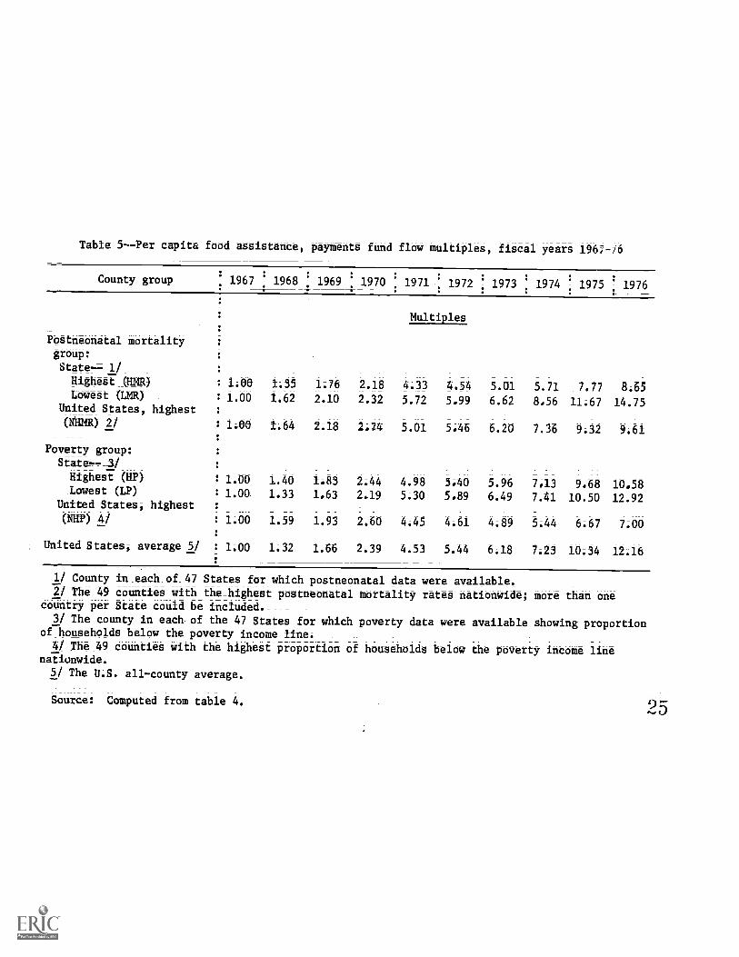
This procedure yielded the multiple bY_WhiCheach year's assistance was greater
than the per capite_food assistance payments received in 1967._ Consequently, fOr the
HMR-CduntieS, the 1976 per capita food assistance payment received was 8.65 times
greater than the 1967 payment. The corresponding multiple for the LMR counties was
14.75.
These data seem_to suggest that the amounts paid shifted in favor of the LMR and
LP countiesin relative terms, particularly after 1970. However, too literal an
interpretation of these data could:be misleading as the magnitude -of the multiples is
a_direct function:of:the size of the bead used in their computation; For example, the
1967 base for bdth LMR and,LP:categories is $2.04, whereas the corresponding amounts
ftir the-Other categories ranged from $4.47 to $12.83 (table 5). The smaller the base,
the easier it is to get a large multiple.
To minimize base-related distortionsi_we calculated the percentage change from
one year to the nexti(table 6). Specifically, the-absolute dollar difference from
1967 to 1968 wasidiVided by the total payments received in_1967- For example, theaverage per capita payment in HMR:counties was $8.88 in 1967. The payment- received in
1968 was $12.01. Consequentlyi_($12.01-48.88)-,/ ($8.88) equals a 35.2 percent
increase in the payment received between 1967 and_1968;__Between_1968 and 1969, the
corresponding computation is: ($15.59- $12.01) / ($12.01) or 29.8 perCent;
An_increase in the absolute payment received for all counties for eaChcifthe__
years reported is indicated by data in table_3. Table 5 shows that -the multiples for
each year likewise increased. In contrast, data-it-table 6 show that, in terms of
relative percentage:increases,_the increase was greater for LMR and LP counties than
for HMR- and -HP counties for some years. For example, the percentage increase for HMR
counties was greater than the percentageihdreage for LMR and LP counties for 1 year;
for 2 years, they were of equal size; and for 6 years, including 1974=76, they were
lower.
Similarly, the annual percentage increase for the HP counties for 5 years was
less-than-the corresponding increment for LMR counties; it-1466 greater for 3 years,
and the same size for 1 year,____The increment for HMR counties was greater than the
corresponding increment for LMR counties for 4 years, but was less for 5 years
(table 6).
Furthermore, the annual increase in food assistance payments to HMR counties
compared -with LP counties showed the_following resultS: for 6-years; the increase in
HMR payments was lessvfor 3 years, it,WAS-mort; in counties received smaller
increases in 5 years; in 4 years, their annual increments were greater. In comparison
With NHMR counties; increments were less in 5 years_and more in 4 years; If this
pattern should persist, after a few years, the absolute distribution in favor of the
HMR and HP (the neediest) counties would shift against them.
Before the Food Stamp Program replaced the Commodity Distribution Program in
1970, the_total number of eligible persons and:the proportion_of eligible persons
participating were typically- greater in HMR and HP counties that in LMR and LP
counties. 4/ With the establishment of the Food Stamp Program in all counties, the
number of eligible persons and thereby the proportion_of participants in LMR and LP
counties increased; Thus, the size of per capita food assistance payments in the_LMR
and LP_counties increased_ after 1971; reflecting the growth in the total number of
partidipahtS; If the post -1972 percentage increases should continue, the least needy
41 After 1970;amajor switch in program emphasis occurred. The Direct Commodity
Distribution Program was continued, but it was directed primarily toward- persons
participating in other programs, particularly the National School Lunch Program;
15 "'LI
Table 5--Per capita food assistance, payments fund flow multiples, fiscal years 1967-16
County group 1967 1968 ! 1969 ! 1970 ! 1971 ! 1972 1973 ! 1974 ! 1975 1976
United States, average 5/ : 1.00 1.32 1.66 2.39 4.53 5.44 6.18 7.23 10.34 12.16
1/ County in each of_47 States -for which postneonatal data were available.2/ The 49 counties with_the_highest postneonatal mortality rates nationwide; More than one
country per State could be included;____
_31 The_county in each. of the 47 States for which poverty data were available ShOWitig propOrtionOfhOUSeholdS below the poverty income line
4/ The 49 counties with the highest proportion of households below the poverty income linenationwide.
5/ The U.S. all-county average.
Source: Computed from table 4.
Table 6 -- Year -to -year increments in per capita food assistance payments, 1967-76
United States, average 5/ : 32.5 25.0 44.3 89.4 20.2 13.5 17.0 43.1 17.6
1/ County in each of the 47 States for which postneonatal data Were available.2/ The 49 counties with the highest postneonatal mortality rates nationwide; more than One
county per State could be included.3/ The county_in each of the 47 Statea for Which poverty data were available showing proportion
Of households below the poverty income line.4/ The 49 counties with the highest proportion of households below the poverty income line
nationwide.
5/ The U.S. all - county average;
Source: Computed from table 4.
27
counties would gain proportionately more. However; this trend appears unlikely.Revised eligibility rules specified by the 1977 Food and Agriculture Att that lowerthe level of income below_which_persons are eligible will particularly affect LMR andLP counties; They will likely lege more participants than will HMR and HP counties;
IMPACT ON RETAIL FOOD SALES
The substantial relative increases in dollars received by HMR and- HP-counties arehighlightedby_the data in table 4. However; the question remains as to whether thesedollars actually increased spending for feed.- DiSbUrSeMeht6 in the form_ofcommodities or of contributions_ to the National School Lunch Program would not beexpected to increase retail food Sales. However; bonus food stamps would;
The total value of bonus stamps distributed in the HMR counties equalled 12percent of-total retailifood Sales (computed fromIFNS_data and 12). This figure;however; cannot be interpreted -as the-gross tentribUtioh to retail foodisales. Eventhough_bonus food stamps are_spent for food in retail food stores; some dollarsformerlyspent-forfood areilikely substituted for nonfood items. In September 1976;the average participating household paid nearly 19 percent of its gross income toreceive free -bonus stamps (16). :If prior to participating; households_ spent more thanthis amount ferfood, then the difference between 19 percent and the proportionactually spent for food was freed for other purchases.
Research_ evidence indicatesthat bonus_stampsappear to be between 40 and 60percent effective in- increasing feed-ekpehditUre6 O. Even when an allowance ismade for such substitution; the contribution of food assistance payments to retailfood sales in a market area should be measurable.
_ We adopted a multiple: regression model to help quantify the relationahipSibeNeenchanges in perlcapita retail feed sales andithe amount of per capita food assistance;We applied this model independently for each -of the six county data sets identifiedearlier. Results_from the regression analysis provide a quantitative basis forevaluating the folloWing four hypotheses:
(1) Bonus food_stamp regression coefficients for HMR and HP counties will besubstantially larger thah corresponding ones for LMR and LP counties. Allcoefficient signs will be positive:
(2) Bonus foodstamp_regresition coefficients for HMR and HP_county_sets will belarger than the corresponding ones for LMR and LP counties. All coefficientsigns will be positive.
(3) Coefficients for the food programs buying_fodd for direct diStribution fromfarmers; wholesalers; and manufacturers will be smaller than the bonus foodstamp coefficients. Indeed, the signs will be negative instead of positive.
(4) The coefficient for disposable personal income (Adjusted Buying Power) willbe smaller than that for behus food stamps. The sign will be positive;
Estimation Method
For purposes of parameter estimation, we tested the data set developed for thisstudy as a dynamic crosssection and expressed variables for -all computations in "realdollars" on a per capita basis; The model may be repreSehted as fellows:
2818
B +Yit
Where:
i = 1, 2, . . N cross sections,
t = 1, 2; T time periods.
That is, the-sample-data are represented by observations of K variables from Ncross-sectional units over T rime periods_._ Given such a data set, the usual ordinaryleast squares assumptions.regarding normally distributeds-homoscedastic,ndnonautoregressive disturbances are highly suspect; In addition to the serialcorrelation problems often encountered in time series data, it is likely thedisturbance structure will:be substantially different-from-the disturbances of asingle-cross-section-over-time. If the disturbances are homoscedastic and/orautoregressive, the parameter estimates obtained from an ordinary least squares (OLS)estimation over the pooled data will be unbiased but inefficient. That is, if thesampling variances-of the-coefficients are obtained from least squares formulas, theywill likely be underestimated. Thereforeiithe_use of either the t or F testsassociated with the OLS estimates is technically invalid for model evaluation. 5/
To cope with such problems, we adopted Park's error components model (5). Morespecifically, the regression equation was:
RFS_ = f (BSPs__- ABP-e)Ps Ps
where:
RFS- = retail food sales per person within a specified county,
B Sp = redeemed bonus stamps per person within the specified county,
Fp = commodity distribution per person within the specified county,
ABP- = adjusted buying power per person Within the specified county; and
e= error component.
The Data
A -10 -year historical record for income; retail food sales, and assistance fromdomestic food programs_was:tabulated for_each county. Net sales data for retail foodestablishments included sales of all products sold-in-foodstores,_both food andnonfood.- We- derived-retail food sales (RFS) by taking the total-sales of countyretail foodstores, as reported in the_Survey_of Buying Power 01), and applying anestimate-of-the percentage of sales allocated to food, published- annually bySuvetwatketAnk-(11). Foodstores were defined as establishments selling food primarilyfor home consumption. Included were sales from grocery stores; meat and fish markets;fruit and vegetable markets; candy, nut, and confectionery stores; dairy productstores; retail bakeries; and egg and poultry dealers;
5/ For additional detailed; discussion of these problems, see (4, 5, 6, and 20).
19 29
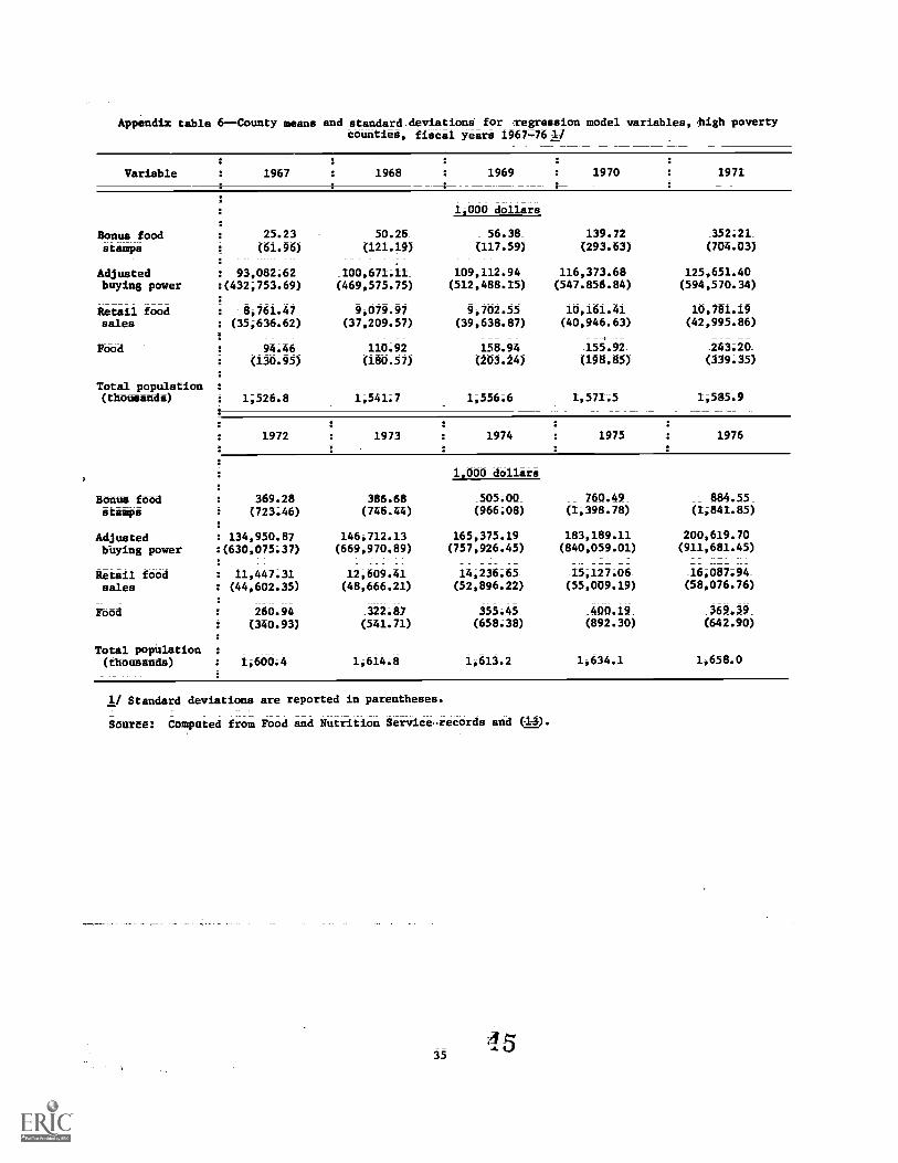
Appendix tables 1 through 8 present county means and_associated standard:deviations-for-each of- -the regression variables. Retail food sales in LMR and LPcounties increased from $22.8 million and $80.8 million; respectively; in 1967; to$44.1 and $162.6 million4 respectively; in_1976:(app. tables 1 and 2). In contrast;sales in-the-NEP-and-NHMR counties amounted-to $4.3 and $5.3 million, respectively; in1976 (app; tables 5 and 6); These data were supplied by ENS.
Bonus food-stamps represent the Federal assistance dollars available foribuyingfood after payment of the purchase requirement; In 1967; the average bonus stamppayment_rangedifrom $7,900 per county -in LMR counties to $85;100 in NHP counties (app.tables 1-and 6). -By 1976, however, the real value of bonus stamps adjusted forinflation in all but the LP counties varied only slightly; Average benefit paymentsfor LP counties were more than three times those 'received in NHP counties.'Undoubtedly; this is- attributable to-substantial differences in-population amongcounty sets. - -In 1976, -for example; total population in LP counties was 14.3 million(app. table 2) versus 3.8 million in LMR counties (app. table 1). There were fewerthan 1,7 million residents in each of the remaining four county sets(app. tables 3-6).
The_sumof_cash reimbursements made-by the Federal-Gbvernment to schoolsparticipating:in the National School Lunch Program, plus all commodities distributedto persons and to institutions; was used as a variable (FOOD). Food program data weresupplied by FNS;
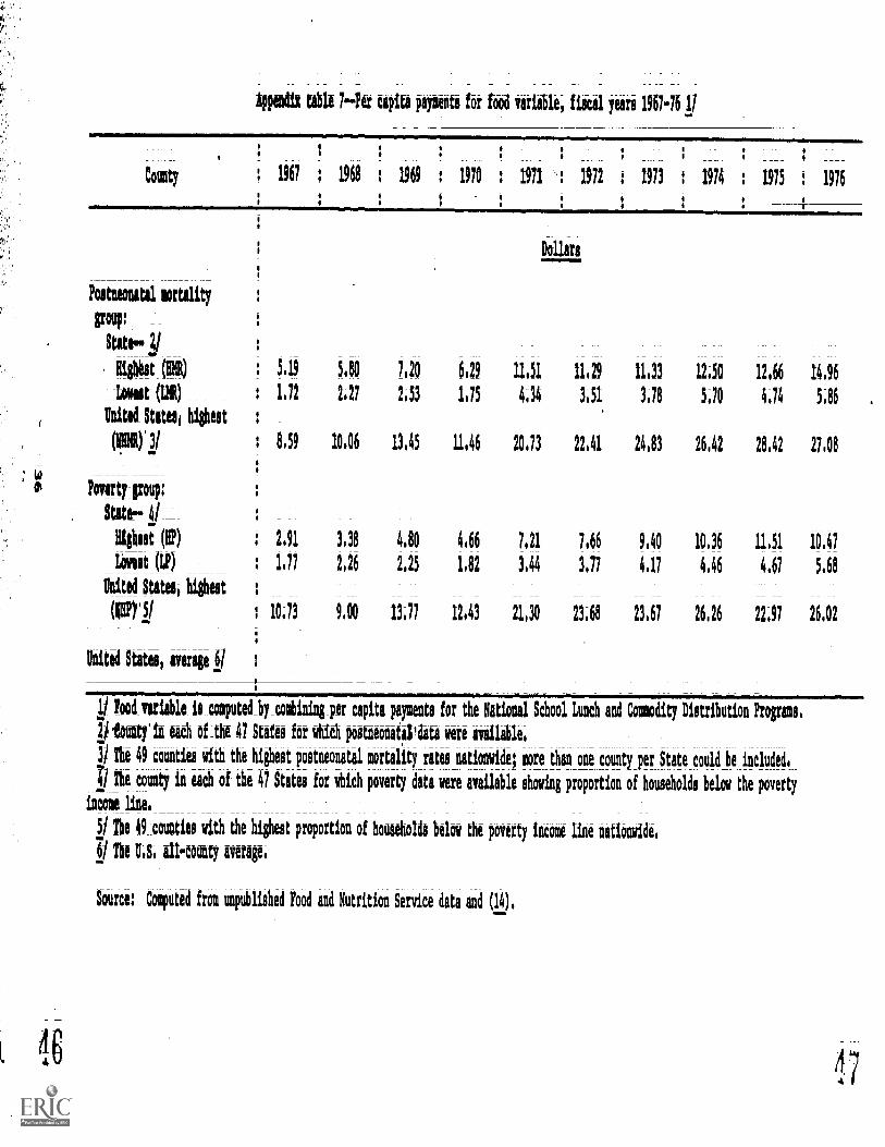
The importance of population size in comparing the per county values can be seenwhen we examine the -FOOD variable. The data in-appendix-tables 1 through 6 revealthat; with the exception of the LP counties; there is little variation in the averagefood:program benefits received, However; data in appendix table 7 indicate that percapita_payments to-NW-and NHMR-counties far exceed those to theremaining_counties.In 1976, NHP and NEMR participants received.FederaI assistance via the National SchoolLunch and Commodity Distribution Programs valued at $26.02 and $27.08 -per personi_respectively. In contrast, benefits in HP and HMR counties were $10.47 and $14.96versus $5.86 and $5.68 in LMR and LP counties (app. table 7);
The_income_variable-was-derived-from the effective buying income (EBI) datacontained in the Survey of Buying Power (II); EBI is disposable personal income lesscompensation paid to-military:and diplomatic-personnel overseas. The_EBLincludes_transfer payments. Consequently, we adjusted this-amount by subtracting bonus foodstamps_from EBI for each county. _Adjusted buying power (ASP) thus represents incomeavailable fOr-food and other purchases; without doUble counting Federal assistanceprovided by food stamps;
ARP in the LP counties was substantially greater than in the remaining counties;ranging from $927 million in 1967 to $2;013 million in 1976 (App. table 2).Predictably; NHP counties had the lowest purchasing power, $34.2 million in 1976 (app.table 4).
Anal-Y-tiCa] Context
The data used for these regressions were not collected within the context of atightly controlled experiMental-design. For example; population changed annually bothin size and age distribution. While the Consumer Price Index for food was used todeflate all dollar_figures; changes in the price level due to noninflationary sourceswere not controlled.
TabIe_7 shows -the change in total population for each of the six county setsbetween 1967 -76, the range in population size among counties constituting each set;
1/County in each of the 47 States for which postneonatal data were available.__/The 49 counties with the highest postneonatal mortality rates nationwide; morethan one county per State cauld be included.3/The:county in each-of the 47 States for. which poverty data were available showing
proportion of households below the poverty income_line.4/The 49 counties with the highest proportion of households below the poverty income
line nationwide.
Source: Compu'A from unpublished Food and Nutrition Service data.
and the average population per square mile for 1972. These data indicate that NHMRand NHP counties-were-the least popUlous and had the lowest population density persquare mile. Furthermore; the change in average population ranged from 4 to_13percent; the_largest LP counties gaining the most and the smallest NHP countiesincreasing the least (table 7).
From these data; we infer that the proportion of the total population in NHMR andNHP counties participating in food programs was substantially greater than in LMR andLP counties; Consequently; the effect of food assistance programs on per capitaretail food sales in NHMR and NHP counties shoUld be more evident than in LMR and LPcounties. The same relationships should hold for HMR and HP counties;
Convential viewpoints on retail food-sales, supported by undeflated time seriesdata; portray continued escalation of retail food sales during the_past decade.Deflated -data (1967 dollars) suggest a somewhat different picture (table 8). In eachof the six data sets, figures in constant 1967-dollars show that, for at least 40percent of the years in the decade; county retail food sales in real dollars were lessthan in 1967. Table 8 indicates that in terms of year-to-year comparisons, for eachof thesik data sets, the following year's total- retail food sales were greater thanthose for the preceding year only 53.7 to 59.1 percent of the time. In facti only forthe NHMR set did as many as seven counties have even 5 consecutive years (1971-76)with such a sequence. DUring this period, 10 counties had real total food sales lower
21
Table 8--Total retail food sales: Specified comparisons of county sets, 1967-76
then-the preceding- year's in at-least 3 of the last 5-years. Also,-in terms of tealper capita retail food sales,_four of the six county_sets in -1976 had either anincrease over corresponding -1967 sales of less than 10 real dollars or an actualdecrease. Two county sets had real per capita increases of between 18 and 19 dollars(app. table 8). Such data do not yield high coefficients of determination.
Empirical Results
The regression model was constructed to explain observed changes in per capitaretail -food sales (in 1967 dollars). Results (in constant dollars) show for -each-dollar's change in average per capita retail food sales how much may be attributed tobonus food stamps, other food assistance transfers; and adjusted buying power. We useresults from the NHP counties to interpret data for each of the other county groups.
Bonus Food Stamps
In NHMR counties, of each dollar's change in per capita retail food-sales, 15;8cents may be attributed to food bonus stamp transfers; 1.8 cents to transfers from theNational School_Lunchand Commodity Distribution programs; and12.1 cents -to adjustedbuying power. Thus, almost 18 percent of each dollar's change in per capita retailfood sales was linked to: food assistance payments, 2 percent to adjusted buying power,and 80 percent to unidentified variables.
The association between bonus food stamps and retail food sales was less strongin other county groups. illoweveriithe coefficient_ for real bonus food stamps waspositive for NHMR, NHP, HMR0and HP county-seta; it was negative for the LMR and LPsets. All coefficients, except those for the HMR set, were statistically significantat the 5percent level, or below. The food stamp coefficients for the NHP and NHMR
22 32
county categories (10.0 cents and 15.8 cents) 6/ were larger than those for the HMRand HP county sets (1.9 cents and -4.0 cents)- -and the LMR and LP categories (-0;1 centand -8.2 cents); see table 9. With respect to coefficient size these data_support ourhypotheses concerning the relationships between changes in -per capita retail foodsales and the amount-of per capita food assistance (see p.18) However; twounanticipated results require explanation. The signs for_the_LMR and LP_sets werenegative, and the HMR coefficient was not statistically significant fot bonus foodstamps.
Each of -the following_ county conditions would contribute to the statistical-estimation of a negative sign for the bonus food stamp coefficients for the LMR and LPsets:
(1) A-very small proportion of the county's total population receiving foodassistance during the observed period.
(2) A substantial number of years during which the following year's average realretail fond sales per person were less than those of the preceding year.
(3) Relatively few years during which the county had participated in the FoodStamp Program.
(4) A substantial proportion of the population residing on an Indianreservation. 7/
The LMR and LP county sets had a larger total population and a higher populationdensity than did any other county set (table 7). For these counties, a smallerproportion of the total population- used- bonus-food stamps. Of those using the bonusfood stamps, it is very likely that a high proportion of these participants receivedthe smaller; rather than the larger; amounts of bonus stamps. This situation occursbecause these hong-eh:Ada are likely to fall within income groups that approach thecut -off level for income eligibility;
For the LMR county set, the-following year's total food sales were less than thepreceding year's in 43 percent of cases; The correspondingJigure:for the LP:countyset was 46 percent. In only five counties did total retail food sales-exceed- -those
during the_praceding year for as-many as 5 consecutive years. Total retail_food saleswere less than those during the preceding -year for 9-_LMR counties_and for 11 LP
counties. _For_both groups; in at least 47 percent of the observediyear8; real totalretail food sales Were less than those reported for 1967. In addition; 12_LP counties(25.5 percent) and 15 LMR counties (32.0 percent) participated in the Food SteMpProgram for 5 years or less in the 1967 -76 period.
The explanation for_thelack_of statistical significance for the HMR county setis similar tothat for the LMR and,LPsets. Fifteen -of the 47 counties in the HMR set
participated in the Food Stamp Program for 5 years or less; Of these 15 counties, -6
had a large Indian population. For example, Roosevelt County; Montana; had a tetelpopulation of 10,635 in 1970. According to the U.S. Department of Interior; over 20
6/ The coefficient for the 49 NHMR set illustrates -how -each of these bonus foodeCaMp-toeffitientg may be interpreted; For each additional dollar of -bonus foodstamps spent; the average±retail:food sales per_person increased by 10.0 cents ( ±1.9
cents). This concept includes all persons residing in the county, not just thosereceiving-bonus food stamps.:
7/ Persons residing on:Indian_reservations frequently preferred the COMMOditybiStribution ProgkaM._ When food stamps replaced distributed commodities; the rate ofparticipation in the Food Stamp Program rose slowly;
23
Table 9-- Results of regression analysis using Park's error component model; 1967-76
*This is the only coefficient that was NOT statistically significant at the 5-per-cent level or below.
1/ Figures in parentheses are standard errors. If reported with the value of(Om), it means-they-were-too low in the fourth decimal place to round upward.2/ The 49 counties with the highest postneonatal mortality rates nationwidet more
than one county per State could be included.3/ The-County in.-each-of the 47 States for which poverty data were available showing
proportion of households below_ the poverty income line. _
4/iThe_49 counties with the highest proportion of hbusehOld§ below the pOVertyincome line nationwide.
Source: Computed from unpublished Food and Nutrition Service data.
24
percent of this county's population is of Indian origin (18); Todd County, SouthDakota; is part of the Rose Bud Indian Reservation.
The Indians- favored the Commodity Distribution Programs and were slow toparticipate:in the Food_Stamp Program. :Ofithe_47 counties in this-set,32.0 percentparticipated less than 3 years-during the-decade. The weight of these 15 counties wasapparently sufficient to result in a low coefficient estimate and a high standarderror. Nevertheless, the weight of the last 4 years was sufficient to result in apositive sign.
The_results_reported here are not directly comparable to those reportedpreviously by Nelson (-9) and Reese (4-0-) for the following three reasons:
(1) The earlier studies used actual, not real, dollars.
(2) The earlier studies refer only to bonus stamp dollars, whereas the_equationhere includes additional food assistance, some of which enters food marketsat wholesale and manufacturing levels.
(3) These real retail sales dollars were computed by dividing -tots l retail foodsales dollarsby the county's total population, not just by the number of itsfood stamp participants;
The Food Variable
Commodity purchases made by USDA:and by- schools participating -in the NationalSchool Lunch_Program typically_are made at the farm, wholesale, and manufacturinglevels. Such purchases, therefore, usually do not show up in retail food sales forhome preparation.
To -the extent that school lunches substitute for food prepared at hove from foodpurchased from retail foodstores, they reduce per capita retail_ food sales.Consequently, we expected the sign for-the food coefficient to -be negative.Statistical findings confirmed our expectations for all but the NHP county set. 8/
Previous surveys have shown- that when school lunch programs are small and arelocated in small communities, food for lunches is often purchased from localretailers, The NHP county set had an average population density of 26 persons persquare Mild;
Direct purchases from local retailers could result in a positive coefficient.However, the data obtained in this study are not sufficient to confirm thishypothesis.
For every dollar distributed through the combined National School Lunch (Federalcash reimbursements) and Commodity Distribution Programs_in NHMR counties, total percapita real-_retail food sales declined by 28.2 cents (+3.6 cents). The correspondingstatistics for the-HMR and HP county-sets were--$1.55 (74- 16.6 cents) and -25;2 cents(+4;4 cents), respectively;_ For the LMR and LP county sets, they were -11.8 cents.(±2.6 cents) and -26.5 cents (+ zero cents), respectively.
8/ For the NHP county set, the coefficient for the food variable was 1.8 cents andwas statistically significant.
25 35
Adjusted Buying Power
As expected; the sign_ifor the adjusted buying power coefficient-was positive foreach_of the county sets. For the NHMR and_ NHP-sets, the bonus food stamp coefficientwas-larger than for the adjusted buying power coefficient. _Although this result hadalso been hypothesized; the coefficient was found to be smaller for the HNR and HP
sets.
Both the bonus food stamp and the adjusted buying power variables-have astatistically significant coefficient in the HP county set. They differ substantiallyin the-size-of-their standard error, but by much less in the value of the_ coefficient.This difference is related to theismall variations year to year in the value-of theper capita_ adjusted buying power in constant dollars. In contrast, the per capita
average value of the bonus food stamp grant rose sharply during1971-76, particularly
during the last 3 years._ The rapid escalation of the bonus food stamp-value resultedin this variable's coefficient having a wide range of values and, consequently; a muchlarger standard error.
During the second decade of the Food-Stamp Program, the average per capita bonusfood stamp-grant should stabilize; At that point, the probability is great that thevalue of the coefficient of the_bonus_food_stamp grant will be greater-than thecorresponding coefficient for adjusted buying power'in constant dollars;
CONCLUSIONS
Progress has been made in providing food for poor people inithe United States.On average, households in localities with the greatest need received substantiallymore food assistance-funds-thau-households in areas with higher incomes. Over the
past decade, the increase in retail food sales_per person was substantial in counties
with high postneonatal mortality rates and with the greatest poverty; In all other
counties, the increase was much lower.
3626
REFERENCES
(1) Citizens' loardof_Inquiry into Hunger and Malnutrition in the United States;
Hunger-U--.-SA Washington, D.C.: Community Press; 1968.
(2) Council of Economic Advisers. Economic -Rep-----t-o-c.-19.ideta-_; Table B-49:
Consumer Price Indexes by Commodity and Service Groups; 1939-1977; p. 313.
Washington, D.C., 1978:
(3) Eaitz; E. F. "Update:on National_Survey on Home Gardening." Speech presented tothe American Seed Trade Association; Inc., 94th Annual Convention; LOUitiVille,
Ky., June 29, 1977.
(4) KakWani;_N; C. "The Unbiasedness of Zeliner's Seemingly Unrelated RegreaeiOnEquationsiEstimators;"_Journal of the Amerce= on; Vol; 62
(Mar. 1967), pp. 141=442.
(5) Kmenta; J. Elements of Econometrkea. New York: Macmillan Co.; 1971;
(6) _;_and R. F. Gilbert. "Small__Sample Properties ofof Seemingly Unrelated Regressions;"AseOciatibh, Vol. 63 (Dec. 1968); pp; 1180-1200;
(7) Longeni_K. A.; and_D.i11.__Murphy. M-Uptiate=Of=DOmeatit Food Programs; U.S.
Dept. Agr., Econ. Stat. Coop. Serv.; forthcoming.
Alternative Estimatort-tiaticaI, .
( ) Meyers; Trienah. "Can A Case Be Made- for -Nutrition Education?" Address at theThirdIfiternational Congress, Food Science and Technology; Washington; D.C.,
Aug. 9, 1970;
(9) Nelson, P.-E., and John Perrin. Economic Effects_of the U.S. Food Stamp Program:
Calendar Year 1972 and Fiscal Year 1974. AER=331. U.S. Dept. Agt., ECOn. Reg;
Serv.; 1976.
(10) Reese, Robert B., and others. =Bonus Stamps and Cash-Income-Supplementa. MRR-
1034. U.S. Dept. Agr., Econ. Res. Serv., Oct. 1974.
(11) Sales and Marketing Management. Survey of Buying Power,--JulIssues-19_68-1_977
(July 1968 reports data for 1967). New York, published annually.