Fourth Year Composite materials

Report: Project final ((Carpet plots))

Report No: final Date: 21/5/2013

Submitted to: Dr. Mohammad Tawfik

Name

Mohammad Tawfik Eraky

محمد توفيق أحمد عراقي

2013/2014

2

Contents Carpet plots ..................................................................................................................................................................... 4

Laminate .......................................................................................................................................................................... 4

1. Carpet plot for laminate in plane modulus Ex under inplane load Nx. .............................................................. 4

2. Carpet plot for laminate in plane poisson ratio in x-y plan................................................................................. 6

3. Carpet plot for laminate shear modlus Gxy under in plane load in x-y plan .................................................... 8

4. Carpet plot for laminate bending modulus Exb under in plane load in x-y plan .............................................. 9

5. Carpet plot for inplane poisson ratio v_xy bending modulus Exb under in plane load in x-y plan ................ 11

APPENDEX ..................................................................................................................................................................... 13

MATLAB program code ............................................................................................................................................ 13

Table of figures

Figure 1 Ex versus thickness fraction gamma ................................................................................................................. 4

Figure 2 poisson ratio versus thickness fraction of lamina +45/-45 ............................................................................... 6

Figure 3 shear modlus vs gamma .................................................................................................................................... 8

Figure 4 bending modulus versus thickness ratio ........................................................................................................... 9

Figure 5 poisson ratio in bending loading Exb ............................................................................................................. 11

3

Introduction

The analysis of deformation of laminated composites can be done accurately, once the orientations ,laminate total thickness

have been chosen ,however the analysis methodology presented so far doesn’t indicate how to design the laminate; that is ,it

doesn’t provide a simple procedure to estimate the required thickness ,layer orientations, ideally the designer would like to

follow a procedure ,which starting with the load and the boundary conditions leads to the complete preliminary design of the

laminate .A laminate design consists of material, number of layers ,layer thickness and orientations ,laminate stacking sequence.

The material specification includes resin and fiber types, fiber volume fraction, and fiber architecture in various layers

Most engineers have considerable training and experience in the design of simple structure components, laminate moduli can be

used to take the advantage of this knowledge for the design of the composite structures.

To simplify the design process ,plots of apparent moduli for various laminate configuration can be produced before hand

4

Carpet plots Carpet plots are constructed for a specific material type and fiber volume fraction, E-glass and isophthalic

polyester matrix with VF =0.5 have been used to construct the carpet plots in figures, using in

plane loading relations

Laminate We used laminate composed of 8 laminas symmetric, with the following

Lamina Orientation

0/90/45/-45/-45/45/90/0.

By constructing a MATLAB code, we generate the following carpet plots, we compare the plots with that in

ch.6 in Barbero Introduction to composite materials , as verification

The MATLAB code attached in the appendix

1. Carpet plot for laminate in plane modulus Ex under inplane load Nx.

Figure 1 Ex versus thickness fraction gamma

5

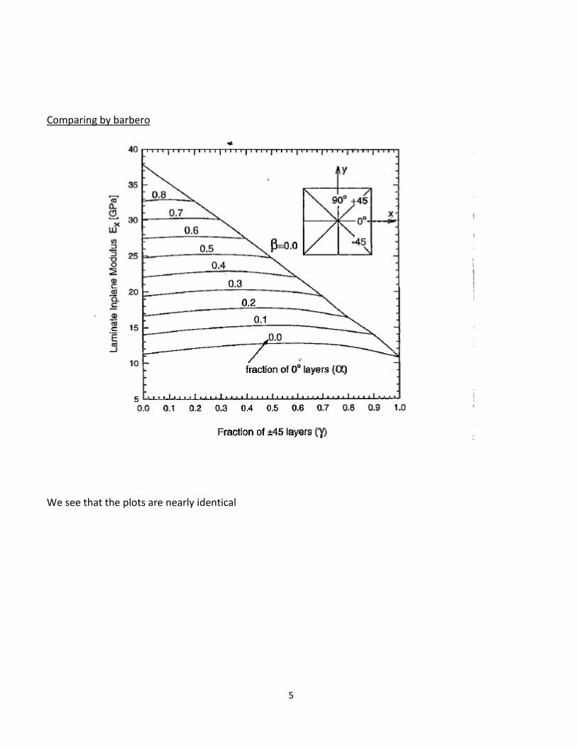
Comparing by barbero

We see that the plots are nearly identical

6

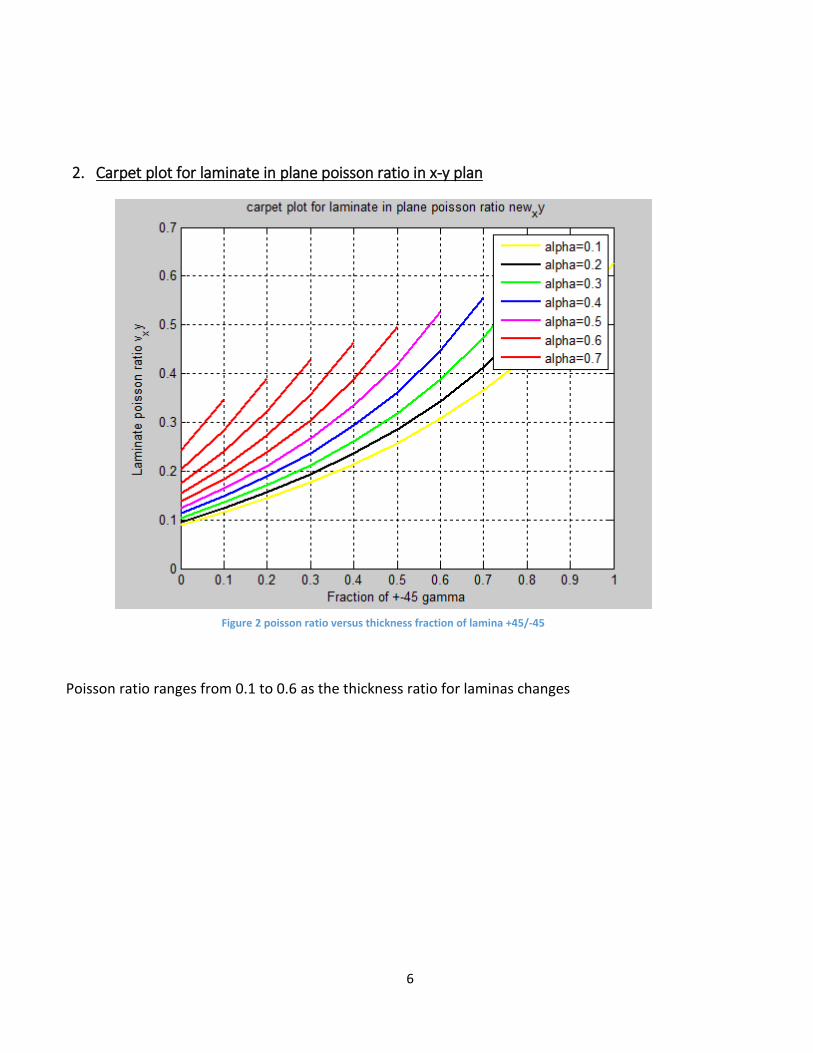
2. Carpet plot for laminate in plane poisson ratio in x-y plan

Poisson ratio ranges from 0.1 to 0.6 as the thickness ratio for laminas changes

Figure 2 poisson ratio versus thickness fraction of lamina +45/-45

7

Comparing by barbero

8

3. Carpet plot for laminate shear modlus Gxy under in plane load in x-y plan

The shear modulus is directly affected by thickness ratio

Figure 3 shear modlus vs gamma

9

4. Carpet plot for laminate bending modulus Exb under in plane load in x-y plan

If we have a lOOk at barber experimental results it’s not nearly the same but still good margin

Figure 4 bending modulus versus thickness ratio

10

Barbero Results

11

5. Carpet plot for inplane poisson ratio v_xy bending modulus Exb under in plane load in x-y plan

Figure 5 poisson ratio in bending loading Exb

12

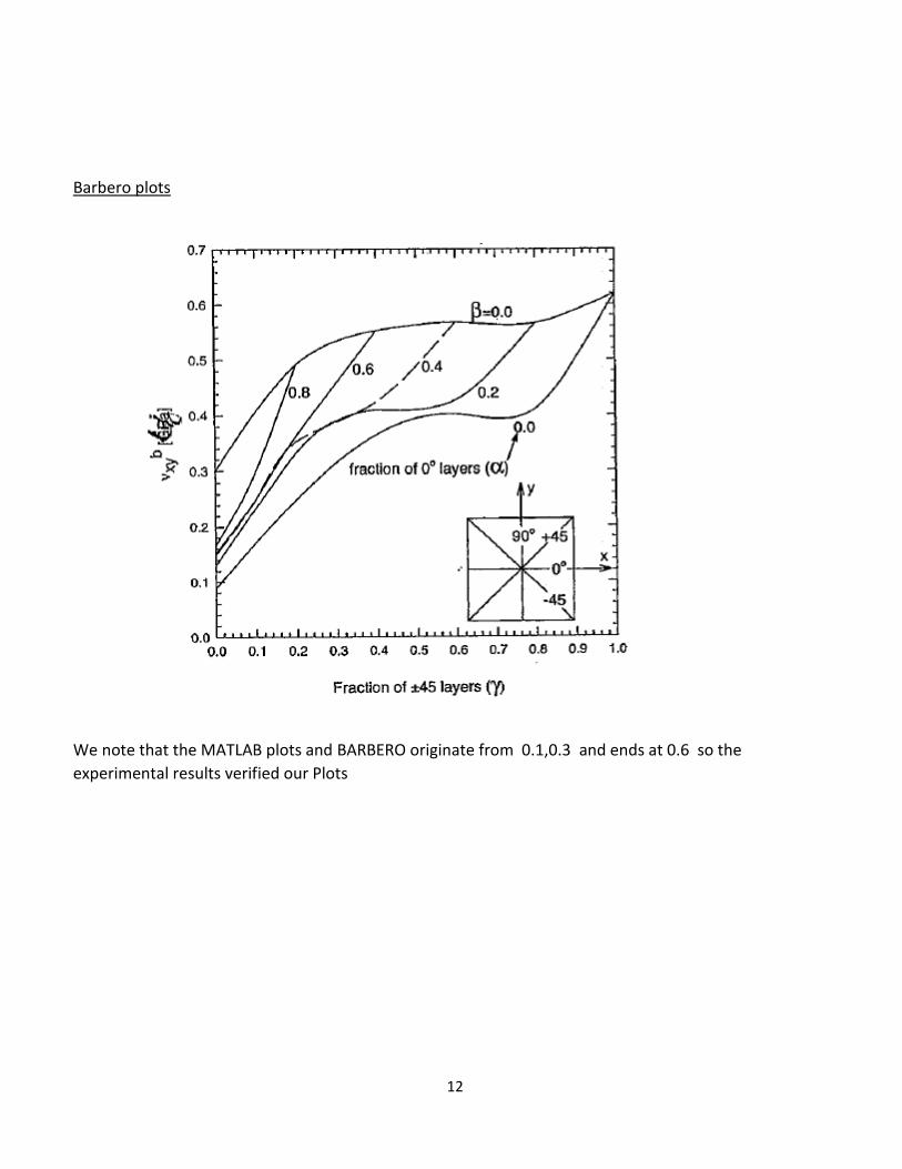
Barbero plots

We note that the MATLAB plots and BARBERO originate from 0.1,0.3 and ends at 0.6 so the

experimental results verified our Plots

13

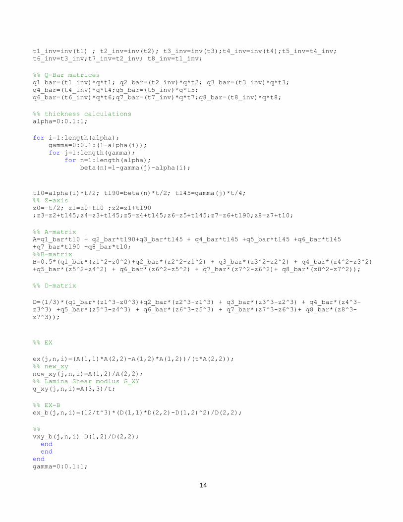
APPENDEX

MATLAB program code clc;clear all;close all ; %% material properities used [ E-glass and isophatalic-polyster matrix with vf=0.5 for

inplane loading] t=16; %total thickness of the laminate e_1=37.9 ; % longitinal modlus Gpa e_2=11.3 ; %transverse modlus Gpa g_12=3.3 ; % inplane shear modlus Gpa new_12=0.3 ;% poisson ratio v_f=0.5 ; % fiber volume ratio new_21=new_12*e_2/e_1; delta=1-new_12*new_21;

%% orientations %in rad ceta_1=0; ceta_2=90*pi/180; ceta_3=45*pi/180; ceta_4=-45*pi/180; ceta_5=ceta_4; ceta_6=ceta_3; ceta_7=ceta_2; ceta_8=ceta_1; %% Q matrix q=[e_1/delta new_12*e_2/delta 0; new_12*e_2/delta e_2/delta 0; 0 0 2*g_12]; %% Transformation matrix

t1=[cos(ceta_1)^2 sin(ceta_1)^2 2*sin(ceta_1)*cos(ceta_1); sin(ceta_1)^2 cos(ceta_1)^2 -2*sin(ceta_1)*cos(ceta_1); -sin(ceta_1)*cos(ceta_1) sin(ceta_1)*cos(ceta_1) cos(ceta_1)^2-sin(ceta_1)^2];

t2=[cos(ceta_2)^2 sin(ceta_2)^2 2*sin(ceta_2)*cos(ceta_2); sin(ceta_2)^2 cos(ceta_2)^2 -2*sin(ceta_2)*cos(ceta_2); -sin(ceta_2)*cos(ceta_2) sin(ceta_2)*cos(ceta_2) cos(ceta_2)^2-sin(ceta_2)^2]; t3=[cos(ceta_3)^2 sin(ceta_3)^2 2*sin(ceta_3)*cos(ceta_3); sin(ceta_3)^2 cos(ceta_3)^2 -2*sin(ceta_3)*cos(ceta_3); -sin(ceta_3)*cos(ceta_3) sin(ceta_3)*cos(ceta_3) cos(ceta_3)^2-sin(ceta_3)^2]; t4=[cos(ceta_4)^2 sin(ceta_4)^2 2*sin(ceta_4)*cos(ceta_4); sin(ceta_4)^2 cos(ceta_4)^2 -2*sin(ceta_4)*cos(ceta_4); -sin(ceta_4)*cos(ceta_4) sin(ceta_4)*cos(ceta_4) cos(ceta_4)^2-sin(ceta_4)^2];

t5=t4; t6=t3 ; t7=t2; t8=t1;

%% Q matrices inverse

14

t1_inv=inv(t1) ; t2_inv=inv(t2); t3_inv=inv(t3);t4_inv=inv(t4);t5_inv=t4_inv;

t6_inv=t3_inv;t7_inv=t2_inv; t8_inv=t1_inv;

%% Q-Bar matrices q1_bar=(t1_inv)*q*t1; q2_bar=(t2_inv)*q*t2; q3_bar=(t3_inv)*q*t3;

q4_bar=(t4_inv)*q*t4;q5_bar=(t5_inv)*q*t5;

q6_bar=(t6_inv)*q*t6;q7_bar=(t7_inv)*q*t7;q8_bar=(t8_inv)*q*t8;

%% thickness calculations alpha=0:0.1:1;

for i=1:length(alpha); gamma=0:0.1:(1-alpha(i)); for j=1:length(gamma); for n=1:length(alpha); beta(n)=1-gamma(j)-alpha(i);

tl0=alpha(i)*t/2; tl90=beta(n)*t/2; tl45=gamma(j)*t/4; %% Z-axis z0=-t/2; z1=z0+tl0 ;z2=z1+tl90

;z3=z2+tl45;z4=z3+tl45;z5=z4+tl45;z6=z5+tl45;z7=z6+tl90;z8=z7+tl0;

%% A-matrix A=q1_bar*tl0 + q2_bar*tl90+q3_bar*tl45 + q4_bar*tl45 +q5_bar*tl45 +q6_bar*tl45

+q7_bar*tl90 +q8_bar*tl0; %%B-matrix B=0.5*(q1_bar*(z1^2-z0^2)+q2_bar*(z2^2-z1^2) + q3_bar*(z3^2-z2^2) + q4_bar*(z4^2-z3^2)

+q5_bar*(z5^2-z4^2) + q6_bar*(z6^2-z5^2) + q7_bar*(z7^2-z6^2)+ q8_bar*(z8^2-z7^2));

%% D-matrix

D=(1/3)*(q1_bar*(z1^3-z0^3)+q2_bar*(z2^3-z1^3) + q3_bar*(z3^3-z2^3) + q4_bar*(z4^3-

z3^3) +q5_bar*(z5^3-z4^3) + q6_bar*(z6^3-z5^3) + q7_bar*(z7^3-z6^3)+ q8_bar*(z8^3-

z7^3));

%% EX

ex(j,n,i)=(A(1,1)*A(2,2)-A(1,2)*A(1,2))/(t*A(2,2)); %% new_xy new_xy(j,n,i)=A(1,2)/A(2,2); %% Lamina Shear modlus G_XY g_xy(j,n,i)=A(3,3)/t;

%% EX-B ex_b(j,n,i)=(12/t^3)*(D(1,1)*D(2,2)-D(1,2)^2)/D(2,2);

%% vxy_b(j,n,i)=D(1,2)/D(2,2); end end end gamma=0:0.1:1;

15

for i=1:length(alpha) C = {'y','k','g','b','m','r','r','r','r','r','r'}; plot(gamma(1:(-i+1+length(gamma))),ex(1:(-

i+1+length(gamma)),1,i),'color',C{i},'linewidth',1.5), legend({'alpha=0.1';'alpha=0.2

';'alpha=0.3';'alpha=0.4';'alpha=0.5';'alpha=0.6';'alpha=0.7'});grid on ylabel('Laminate inplane modlus Ex(Gpa)');xlabel('Fraction of +-45 gamma'); title('carpet plot for laminate in plane modlus Ex under inplane load Nx');grid

on,hold on

end figure for i=1:length(alpha) C = {'y','k','g','b','m','r','r','r','r','r','r'}; plot(gamma(1:(-i+1+length(gamma))),new_xy(1:(-

i+1+length(gamma)),1,i),'color',C{i},'linewidth',1.5), legend({'alpha=0.1';'alpha=0.2

';'alpha=0.3';'alpha=0.4';'alpha=0.5';'alpha=0.6';'alpha=0.7'});grid on ylabel('Laminate poisson ratio v_xy');xlabel('Fraction of +-45 gamma'); title('carpet plot for laminate in plane poisson ratio new_xy');grid on,hold on end

figure for i=1:length(alpha)

plot(gamma(1:(-i+1+length(gamma))),g_xy(1:(-

i+1+length(gamma)),1,i),'m','linewidth',1.5) ylabel('Laminate shear modlus modlus Gx(Gpa)');xlabel('Fraction of +-45 gamma'); title('carpet plot for laminate shear modlus Gxy under inplane load Nxy');grid on

;hold on end figure for i=1:length(alpha) C = {'y','k','g','b','m','r','r','r','r','r','r'}; plot(gamma(1:(-i+1+length(gamma))),ex_b(1:(-

i+1+length(gamma)),1,i),'color',C{i},'linewidth',1.5),

legend({'alpha=0';'alpha=0.1';'alpha=0.2';'alpha=0.3';'5alpha=0.4';'alpha=0.5';'alpha=

0.6'});grid on ylabel('Laminate bending modlus Exb(Gpa)');xlabel('Fraction of +-45 gamma'); title('carpet plot for laminate bending modlus Exb under ');grid on ;hold on end figure for i=1:length(alpha) C = {'y','k','g','b','m','r','r','r','r','r','r'}; plot(gamma(1:(-i+1+length(gamma))),vxy_b(1:(-

i+1+length(gamma)),1,i),'color',C{i},'linewidth',1.5),

legend({'alpha=0';'alpha=0.1';'alpha=0.2';'alpha=0.3';'5alpha=0.4';'alpha=0.5';'alpha=

0.6'});grid on ylabel('Vxy_b');xlabel('raction of +-45 gamma'); title('carpet plot for inplane poisson ratio vxy_b in bending loadin modlus Exb

unde)');grid on ;hold on end