Project Number: MQP-RBM-0601

Reducing Greenhouse Gas Emissions from Asphalt Materials

A Major Qualifying Project Report:

submitted to the Faculty

of the

WORCESTER POLYTECHNIC INSTITUTE

in partial fulfillment of the requirements for the

Degree of Bachelor of Science by

____________________________ Christine Keches

and

____________________________ Amy LeBlanc

Date: March 1, 2007

Approved:

________________________________

Professor Rajib Mallick, Major Advisor 1. asphalt 2. Sasobit® 3. emissions

________________________________ Professor John Bergendahl, Co-Advisor

ii

Executive Summary

Through the construction of new asphalt pavements, the asphalt industry has been

contributing to greenhouse gas emissions released into our atmosphere. Recently, there have

been products developed, such as Sasobit®, that decrease viscosity of asphalt at a lower than

conventional mix temperature, which can in turn reduce greenhouse gas emissions. The

objectives of this study were to determine if emissions can be reduced with the use of Warm Mix

Asphalt (WMA), and whether any material properties can be expected to improve in mixes

produced at lower temperatures (WMA versus Hot Mix Asphalt, or HMA). Another objective

was to determine economic benefits, if any, of producing mixes at lower temperatures.

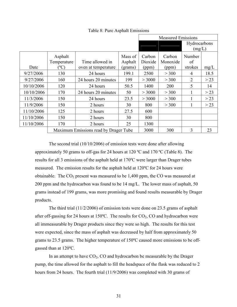
Testing for this study included emission testing for pure asphalt and asphalt mixes. HMA

and WMA samples were also mixed and compacted to test material properties. All tests

completed were done on 3 separate mixes: HMA with 5.3% asphalt, WMA with 5.3% asphalt

and 1% Sasobit® (by mass of asphalt), and WMA with 4.8% asphalt and 1% Sasobit® (by mass

of asphalt).

For all emission tests, Drager testing equipment was used. The set up used for these tests

consisted of flasks, ovens, a Drager pump and Drager tubes. To measure carbon dioxide (CO2),

the Drager pump needed 10 full strokes and it took approximately four minutes for the test to be

completed. The color change in the chemical inside the tube indicated the amount of gas in the

sample in parts per million (ppm). Preliminary testing of emissions emitted from pure asphalt

was done to develop a procedure since there are no test standards for this available at this time.

For this study, approximately sixty grams of asphalt mix, both WMA and HMA, and

approximately twenty-five grams of pure asphalt were tested for emissions.

The three asphalt mixes in this study were tested for both unaged and aged conditions of

material properties according to standards developed by the American Society for Testing and

Materials. The tests conducted to determine volumetric and mechanical properties were Bulk

Specific Gravity, Theoretical Maximum Density, and Indirect Tensile Strength. The volumetric

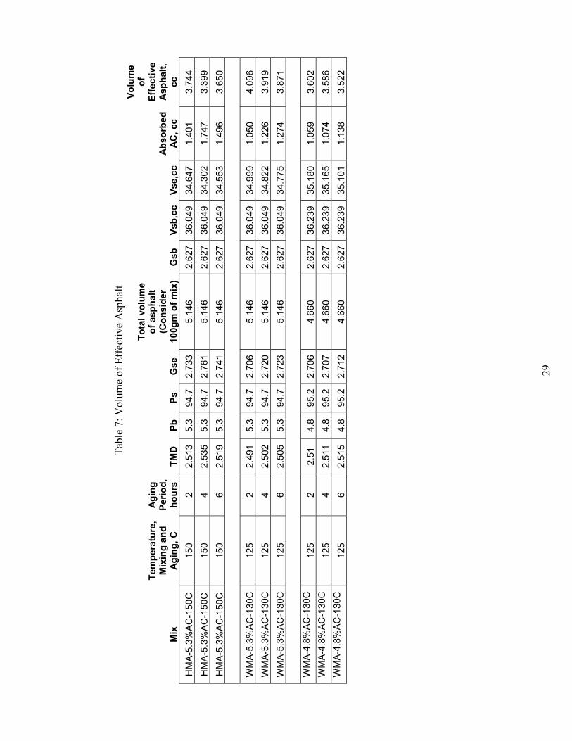
properties analyzed were percent air voids, absorption and effective asphalt content.

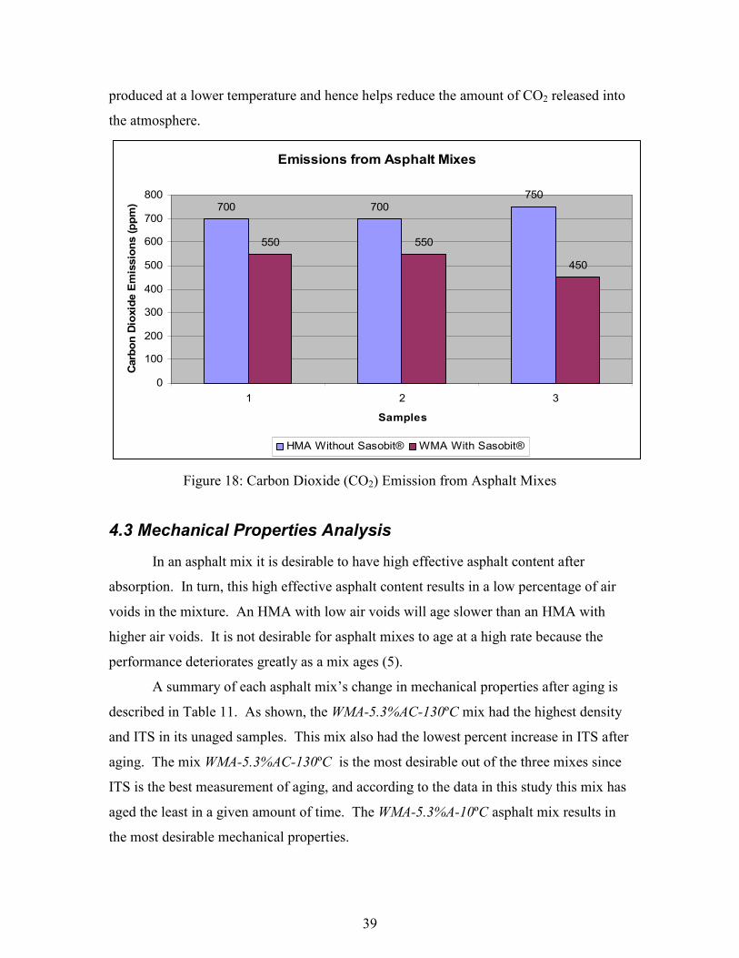
After thorough testing and analysis of the three different asphalt mixes, it is determined

that the additive Sasobit® is a beneficial material to be used in WMA. The changes in material

properties result in stronger and longer lasting asphalt mixes as well as a longer paving season.

With the addition of Sasobit® the temperature of HMA production can be cut down by 20°C and

iii

as a result, the carbon dioxide emissions let off by the asphalt industry could be reduced as much

as 43.9% per year. This includes emissions from the fuel used as well as from the asphalt

materials used to produce the Hot Mix Asphalt. In addition, the decreased temperature required

for Sasobit® asphalt mixes can save over $69 million in energy costs.

The ecological impacts that the use of Sasobit® in asphalt mixes can have for the asphalt

industry are significant. The reduction of greenhouse gases from asphalt mix materials and

energy consumed by the asphalt industry can make a difference in the world we live in and have

the potential to improve the earth’s atmosphere. From this study, it was calculated that 3.774

million tonnes of CO2 could be prevented from being released into the atmosphere per year from

the asphalt mix materials as well as energy used during production. In 10 years, 37.74 million

metric tons of CO2 could be prevented. It is essential for the asphalt industry to start caring

about their effects on the environment, and the addition of Sasobit® to asphalt mixes would be a

great start for this.

iv

Abstract

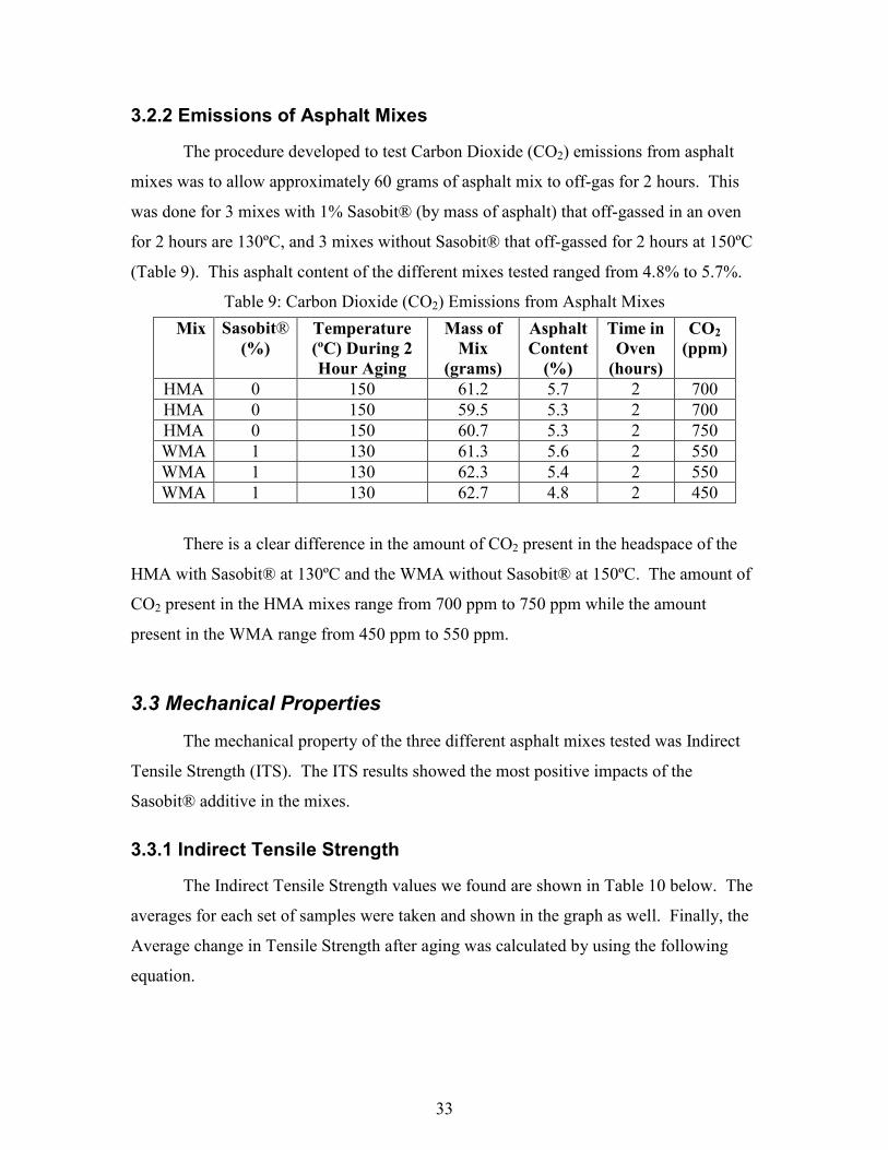
The additive Sasobit® was tested in three asphalt mixes at two temperatures. Volumetric properties, carbon dioxide emissions and mechanical properties were tested to determine if Sasobit® would be an effective additive for the asphalt industry. It was found that the use of Sasobit® in Warm Mix Asphalt can help reduce carbon dioxide emissions, costs and energy used by the asphalt industry without affecting the quality of asphalt pavements.

v

Acknowledgements We would like to thank the following people for helping us to complete this project.

Rajib Mallick, Associate Professor of Civil Engineering at WPI

John Bergendahl, Associate Professor of Civil Engineering at WPI

Donald Pellegrino, Lab Manager

Julie Penny, Graduate Teaching Assistant

Laura Rockett, Undergraduate Lab Technician

Matt Teto, Killingly Asphalt Products

vi

Table of Contents Executive Summary ........................................................................................................................ii Abstract .......................................................................................................................................... iv Acknowledgements ......................................................................................................................... v Table of Contents ...........................................................................................................................vi Table of Figures ...........................................................................................................................viii List of Tables.................................................................................................................................. ix Table of Equations .......................................................................................................................... x Chapter 1: Introduction and Objectives .......................................................................................... 1 1.1 Greenhouse Gas Emissions ................................................................................................... 1 1.1.1 Reducing Greenhouse Gas Emissions............................................................................ 2

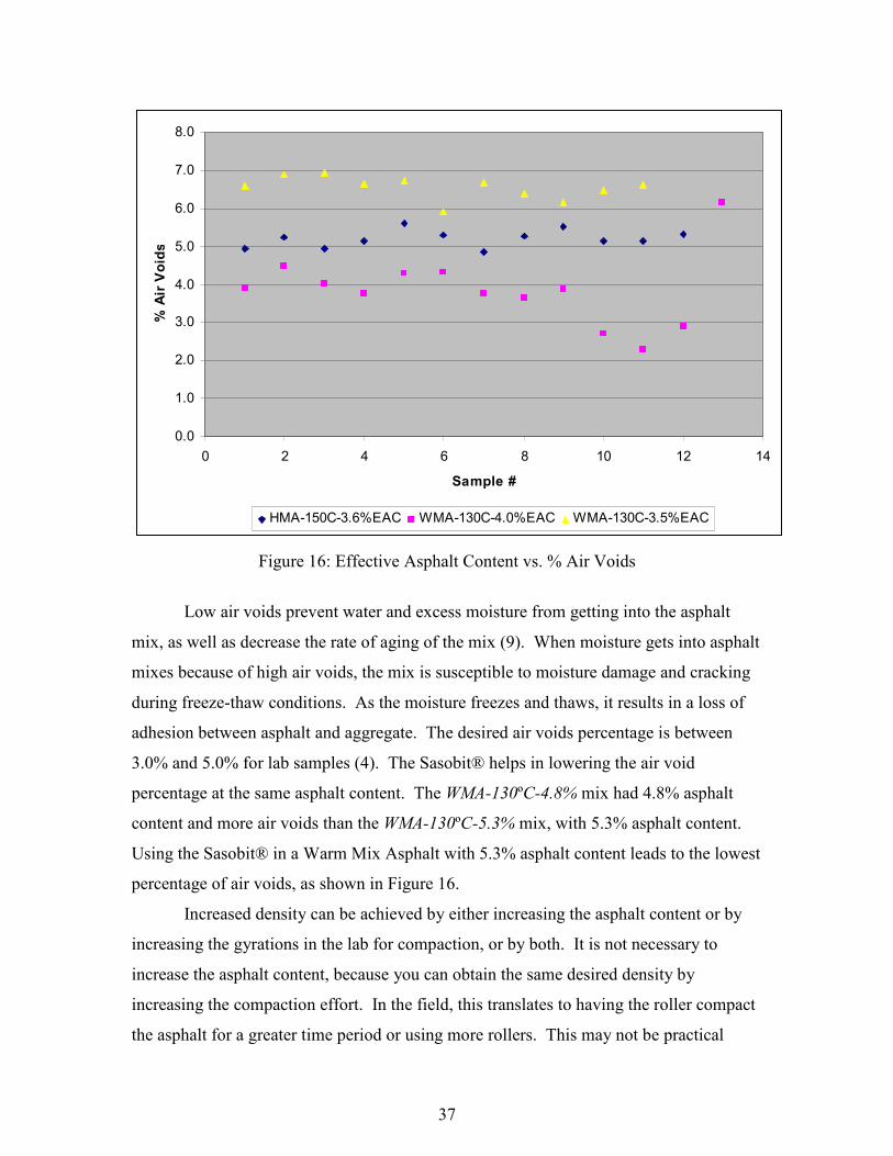
1.2 Asphalt Properties ................................................................................................................. 3 1.2.1 Viscosity and Temperature............................................................................................. 3

1.3 Asphalt Mix........................................................................................................................... 4 1.3.1. Production of Asphalt Mix............................................................................................ 4 1.3.2 Emissions Produced during Construction ...................................................................... 4

1.4 Additives to Reduce Mix Temperature ................................................................................. 7 1.4.1 Sasobit® ......................................................................................................................... 7 1.4.2 Possible Reduction of Mix Emissions............................................................................ 8

1.5 Objectives.............................................................................................................................. 9 Chapter 2: Scope of Work............................................................................................................. 10 2.1 Testing Procedures .............................................................................................................. 10 2.1.1 Drager Equipment for Emission Testing...................................................................... 12 2.1.2 Preliminary Testing Procedures ................................................................................... 14 2.1.3 Mixing and Compacting............................................................................................... 15 2.1.3.1 Sieving Aggregates ............................................................................................... 15 2.1.3.2 4,550 Gram Batches for Compaction and Testing ................................................ 16 2.1.3.3 1,500 Gram Batches for Emission Testing and Theoretical Maximum Density .. 18

2.1.4 Emission Tests of Asphalt Mixes................................................................................. 19 2.1.5 Volumetric and Mechanical Properties for Unaged and Aged Samples ...................... 21 2.1.5.1 Bulk Specific Gravity (BSG) ................................................................................ 21 2.1.5.2 Theoretical Maximum Density (TMD) ................................................................. 22 2.1.5.3 Indirect Tensile Strength (ITS) ............................................................................. 23 2.1.5.4 Aged Samples........................................................................................................ 24

Chapter 3: Results ......................................................................................................................... 25 3.1 Volumetric Properties ......................................................................................................... 25 3.1.1. Percent Air Voids ........................................................................................................ 25 3.1.2 Absorption & Effective Asphalt Content ..................................................................... 27

3.2 Emissions ............................................................................................................................ 30 3.2.1 Emissions of Asphalt.................................................................................................... 30 3.2.2 Emissions of Asphalt Mixes......................................................................................... 33

3.3 Mechanical Properties ......................................................................................................... 33 3.3.1 Indirect Tensile Strength .............................................................................................. 33

Chapter 4: Analysis ....................................................................................................................... 36 4.1 Volumetric Properties Analysis .......................................................................................... 36

vii

4.2 Asphalt Mix Emissions Analysis ........................................................................................ 38 4.3 Mechanical Properties Analysis .......................................................................................... 39

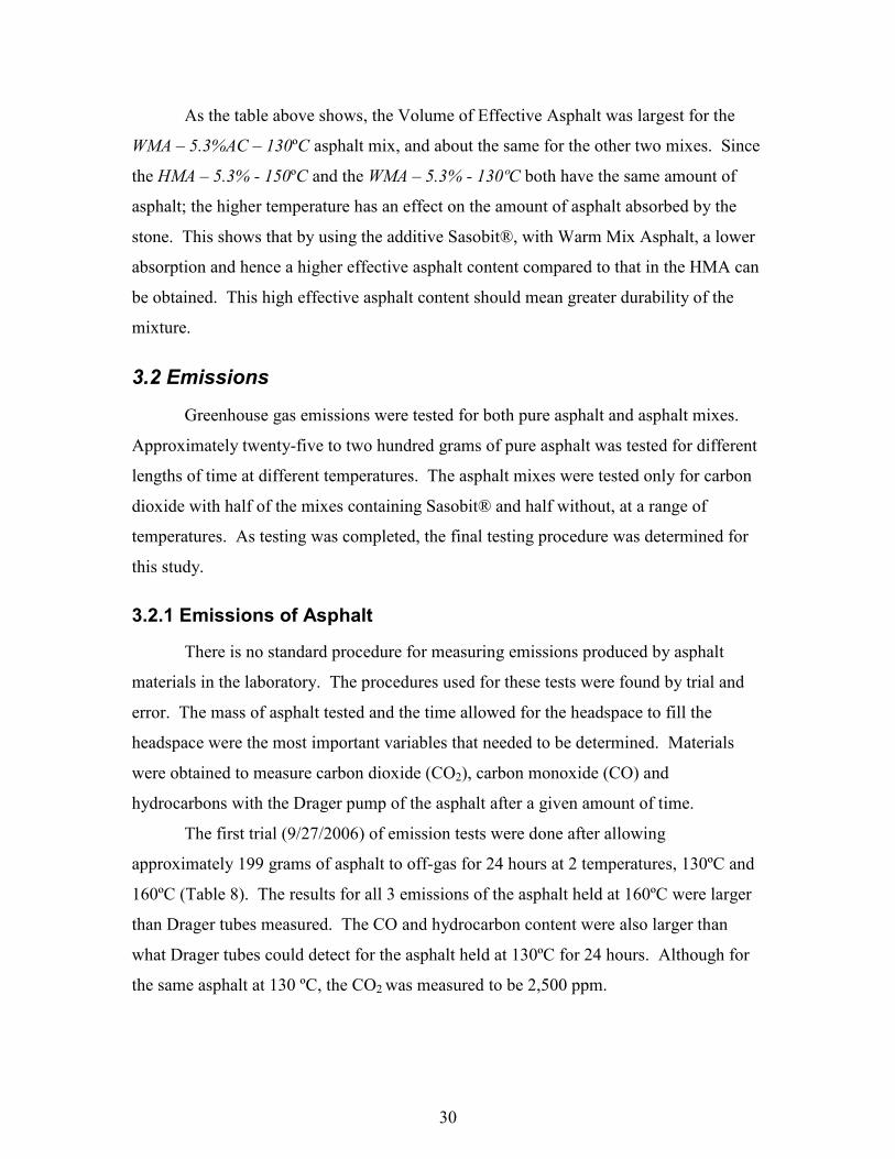
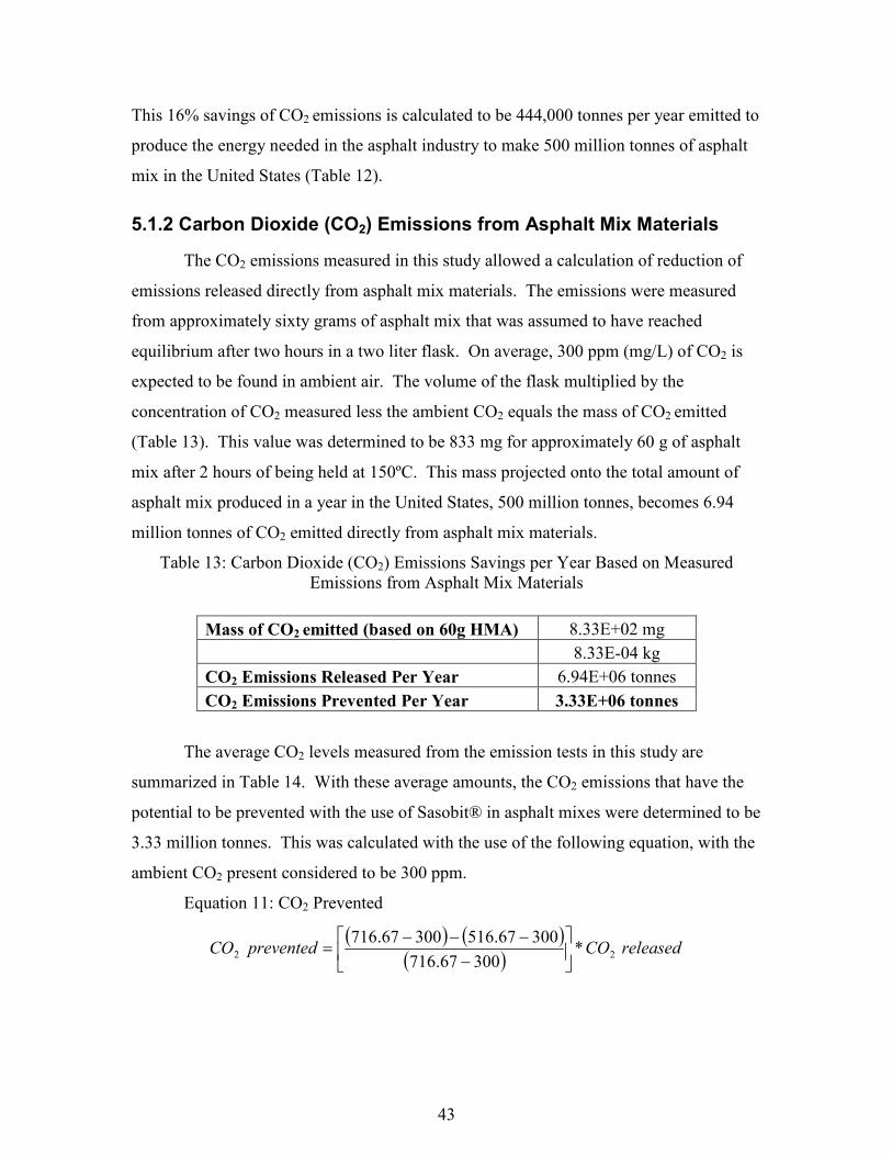
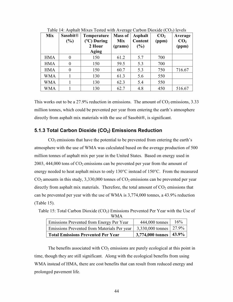
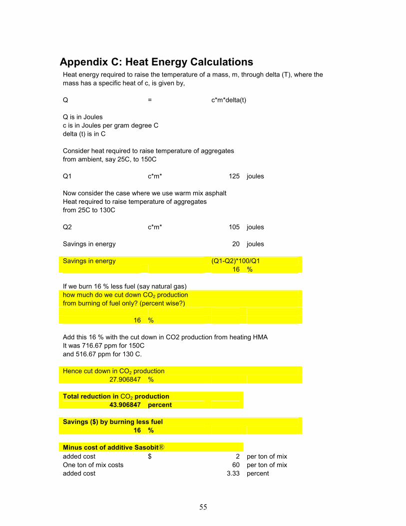
Chapter 5: Benefits........................................................................................................................ 41 5.1 Carbon Dioxide Emissions Reduction from Energy and Materials .................................... 41 5.1.1 Carbon Dioxide (CO2) Emissions from Energy Needed to Produce HMA................. 41 5.1.2 Carbon Dioxide (CO2) Emissions from Asphalt Mix Materials .................................. 43 5.1.3 Total Carbon Dioxide (CO2) Emissions Reduction ..................................................... 44

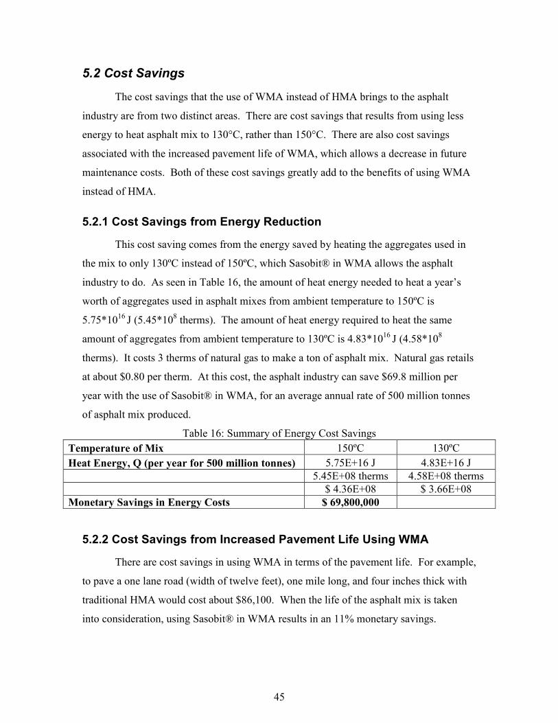
5.2 Cost Savings........................................................................................................................ 45 5.2.1 Cost Savings from Energy Reduction .......................................................................... 45 5.2.2 Cost Savings from Increased Pavement Life Using WMA.......................................... 45

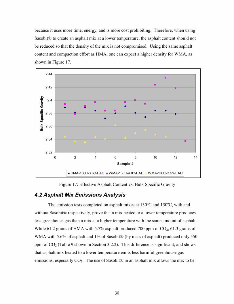
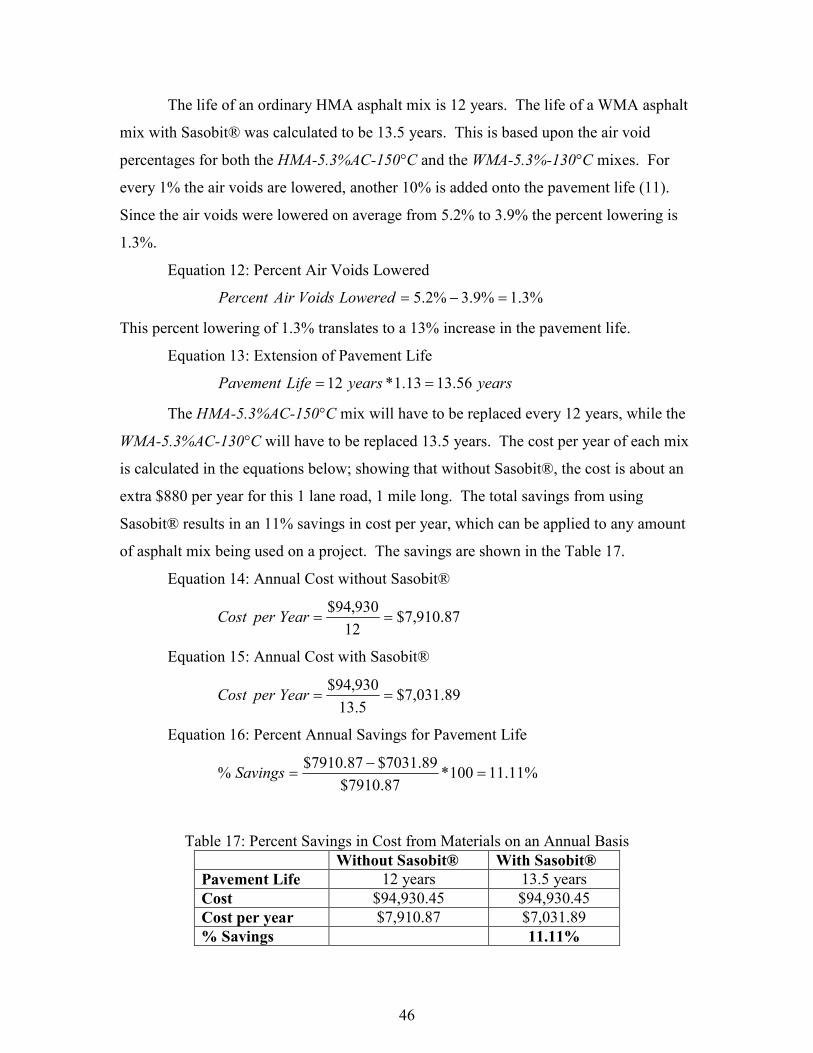
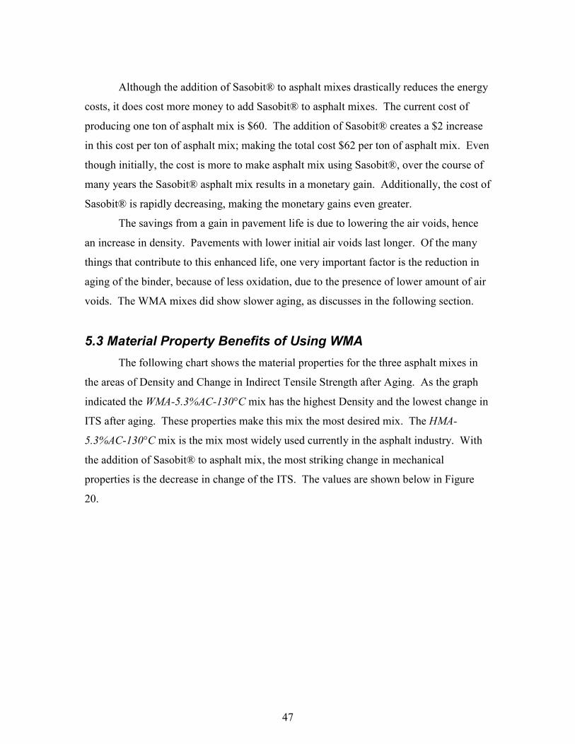
5.3 Material Property Benefits of Using WMA ........................................................................ 47 5.4 Benefits of Extending the Paving Season ........................................................................... 48 5.5 Conclusion........................................................................................................................... 49

Bibliography.................................................................................................................................. 50 Appendix A: Production of Sasobit® ........................................................................................... 51 Appendix B: Testing Flow Charts................................................................................................. 52 Appendix C: Heat Energy Calculations ........................................................................................ 55

viii

Table of Figures Figure 1: Production of Asphalt Map (6) ........................................................................................ 6 Figure 2: Mixing and Compaction Temperature for PG 64-22 Binders (4).................................... 8 Figure 3: Generic Flow Chart of Testing for HMA and WMA .................................................... 11 Figure 4: Drager Testing Materials ............................................................................................... 12 Figure 5: Drager Tube Opener ...................................................................................................... 12 Figure 6: Drager Pump Measurement of Hydrocarbon................................................................. 13 Figure 7: Hydrocarbon Drager Tube............................................................................................. 13 Figure 8: Drager Pump in Flask .................................................................................................... 14 Figure 9: Mechanical Shaker with Sieves ..................................................................................... 16 Figure 10: Mixer............................................................................................................................ 18 Figure 11: Glass Flask and Funnel................................................................................................ 20 Figure 12: Machine Performing ITS Testing ................................................................................ 23 Figure 13: Measuring thickness values for the samples................................................................ 24 Figure 14: Average Air Voids....................................................................................................... 27 Figure 15: Carbon Dioxide (CO2) Emissions of Pure Asphalt...................................................... 32 Figure 16: Effective Asphalt Content vs. % Air Voids................................................................. 37 Figure 17: Effective Asphalt Content vs. Bulk Specific Gravity.................................................. 38 Figure 18: Carbon Dioxide (CO2) Emission from Asphalt Mixes ................................................ 39 Figure 19: Average Change in ITS After Aging ........................................................................... 40 Figure 20: Material Properties ...................................................................................................... 48

ix

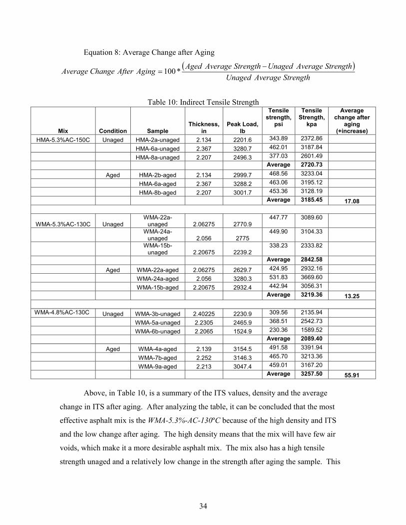
List of Tables Table 1: Blend of 4,550 gram Aggregate Batches ........................................................................ 17 Table 2: Asphalt Mixes Used for 4,550 gram Batches ................................................................. 17 Table 3: Blend of 1,500 gram Aggregate Batches ........................................................................ 19 Table 4: Asphalt Mixes Used for 1,500 gram Batches ................................................................. 19 Table 5: Asphalt Mixes Tested for Emissions .............................................................................. 20 Table 6: Bulk Specific Gravity & Percent Air Voids.................................................................... 26 Table 7: Volume of Effective Asphalt .......................................................................................... 29 Table 8: Pure Asphalt Emissions .................................................................................................. 31 Table 9: Carbon Dioxide (CO2) Emissions from Asphalt Mixes.................................................. 33 Table 10: Indirect Tensile Strength............................................................................................... 34 Table 11: Summary of Mix Mechanical Properties Changes after Aging .................................... 40 Table 12: Carbon Dioxide (CO2) Emissions Savings per Year Based on Energy Needed for

Asphalt Industry .................................................................................................................... 42 Table 13: Carbon Dioxide (CO2) Emissions Savings per Year Based on Measured Emissions

from Asphalt Mix Materials.................................................................................................. 43 Table 14: Asphalt Mixes Tested with Average Carbon Dioxide (CO2) levels ............................. 44 Table 15: Total Carbon Dioxide (CO2) Emissions Prevented Per Year with the Use of WMA... 44 Table 16: Summary of Energy Cost Savings ................................................................................ 45 Table 17: Percent Savings in Cost from Materials on an Annual Basis ....................................... 46

x

Table of Equations Equation 1: Bulk Specific Gravity, Saturated Surface Dry (SSD)................................................ 21 Equation 2: Theoretical Maximum Density, TMD....................................................................... 22 Equation 3: Indirect Tensile Strength, ITS.................................................................................... 23 Equation 4: Percent Air Void ........................................................................................................ 25 Equation 5: Effective Specific Gravity, Gse .................................................................................. 28 Equation 6: Bulk Volume of Stone, Vsb ........................................................................................ 28 Equation 7: Effective Volume of Stone, Vse ................................................................................. 28 Equation 8: Average Change after Aging ..................................................................................... 34 Equation 9: Heat Energy ............................................................................................................... 41 Equation 10: Percent Savings in Energy....................................................................................... 42 Equation 11: CO2 Prevented ......................................................................................................... 43 Equation 12: Percent Air Voids Lowered ..................................................................................... 46 Equation 13: Extension of Pavement Life..................................................................................... 46 Equation 14: Annual Cost without Sasobit® ................................................................................ 46 Equation 15: Annual Cost with Sasobit® ..................................................................................... 46 Equation 16: Percent Annual Savings for Pavement Life............................................................. 46

1

Chapter 1: Introduction and Objectives

Through the construction of new asphalt pavements, the asphalt industry has been

contributing to greenhouse gas emissions released into our atmosphere. Recently, there

have been products developed that decrease viscosity of asphalt at a lower than

conventional mix temperature. These lower temperatures can in turn reduce greenhouse

gas emissions. In addition to environmental benefits, the asphalt industry could greatly

profit from these products. On average 30-50% of the costs at an asphalt plant are for

emission control (1). Companies are limited to specific areas to operate asphalt plants in,

but if emissions were reduced, asphalt plants could be built in areas with strict pollution

regulations. This would mean shorter haul distances to construction sites, less costly

operations, and savings for the tax paying public also.

1.1 Greenhouse Gas Emissions

Over the past few decades, as our culture has become more environmentally

conscious, we have taken more notice to the problem of greenhouse gas emissions.

Greenhouse gas emissions come mostly from the burning of fossil fuels and industry

processes (2). The main emissions that are present in our atmosphere are water vapor,

carbon dioxide, methane, nitrous oxide, and many engineered gases.

Greenhouse gas emissions cause many environmental problems for our earth.

Many gas emissions soak up infrared radiation from the atmosphere, trapping heat in our

lower atmosphere (2). This is called the Greenhouse Effect, and if it were not present the

earth’s natural temperature would be around -19ºC (-2.2ºF). The Greenhouse Effect is

not a negative process, and keeps our earth at a more tolerable 14ºC. However, many

scientists and researchers believe in the process of Global Warming. They believe that

with the increasing amounts of gases emitted into the atmosphere each year, the

temperature of our earth is rising. According to computer-stimulated models, the

increase in gases will always result in Earth’s temperature rising. Although these are just

computer models, the actual temperature of the Earth has increased 0.6ºC over the past

100 years (2).

2

These rising temperatures, of both land and ocean, have the ability to create

changes in our weather patterns on Earth. We have seen a lot changes over the past

decade in our weather patterns and an increase in severe storms and hurricanes. These

changes have yet to be proven a sole result of human activities, as opposed to natural

variations having an impact (2).

1.1.1 Reducing Greenhouse Gas Emissions

The actions taken in response to concerns of Global Warming come from

organizations such as the Domestic Policy Council and the National Academy of

Sciences (2). The National Academy of Sciences through National Research Council

prepared a statement on Global Response to Climate Change. The statement indicates

that not only is climate change real, but it caused by human activity. It went on to say

that nations should begin taking steps to reduce the growth of greenhouse gas emissions,

as well as prepare for future climate changes.

Over the past few years, as an increasing number of people have recognized the

problems associated with greenhouse gas emissions, more efforts have been made to

lower emissions. In 1992, the Energy Policy Act was put in place, mandating the Energy

Information Administration (EIA) to produce an inventory of aggregate U.S. national

emissions updated each year (2). Although this report is useful to recognize our specific

problems, U.S. emissions are still far above what they should be. In 2002, U.S. energy-

related carbon dioxide emissions totaled more than 5,746 million metric tons, making up

approximately 24 percent of the worlds’ total emissions.

There have been some actions taken to control the amount of emissions caused by

asphalt production. Title V of the Clean Air Act, 1990, states that “(it) requires the

accurate estimation of emissions from all U.S. manufacturing processes, and places the

burden of proof for that estimate on the process owner” (3, p.1). Although some general

actions have been taken towards the reduction of greenhouse gas emissions, there needs

to be more focus on improving the asphalt industry.

3

1.2 Asphalt Properties

The majority of paving asphalt cement used at this time is obtained by processing

crude oils (4). Distillation is the first step in processing all crude oil. There are several

techniques to produce asphalt cements with straight reduction to grade being the most

commonly used. The processed asphalt must be workable to be mixed with other

substances, such as aggregates, which requires a low viscosity. This can be achieved by

heating the asphalt to a high temperature (such as 150ºC).

1.2.1 Viscosity and Temperature

Two intrinsic properties that affect asphalt’s physical state and performance are

viscosity and temperature. Temperature and viscosity are very much related to each

other. In order to construct asphalt pavements, the asphalt must be heated to a very high

temperature (150ºC) to get a low viscosity, and thus a good coating of aggregates (4).

The mix also has to be workable such that it can be compacted to an adequate density to

obtain a strong and durable road.

The resistance of flow of a given fluid is defined as viscosity.

Viscosity at any given temperature and shear rate is essentially the ratio of shear stress to shear strain rate. At high temperatures such as 135ºC, asphalt cements behave as simple Newtonian liquids; that is the ratio of shear stress to shear strain rate is constant. At low temperature, the ratio of shear stress to shear strain is not a constant, and the asphalt cements behave like non-Newtonian liquids….viscosity is a fundamental consistency measurement in absolute units that is generally not affected by changes in test configurations or geometry of the samples (4, p. 48-49).

The quantity of light fractions retained in asphalt after processing affects the viscosity

(5). Gasoline, kerosene and fuel oils are types of light fractions. The atomic structure of

the fractions exhibit different behaviors. Even after experiencing the same processing,

asphalts from different sources will contain different amounts of light fractions and have

different viscosities.

Asphalt binder is considered a thermoplastic material (4). The consistency of asphalt

changes according to the temperature it is subjected to. The rate this occurs at is very

important and is referred to as temperature susceptibility. Temperature not only affects

the viscosity of the asphalt, but it also affects the amount of emissions released from the

material. It is impossible to create an asphalt mix unless the asphalt has a relatively low

viscosity. The low viscosity allows the asphalt to coat and mix with the aggregates

4

properly. To obtain the low viscosity it is generally necessary to heat the asphalt and the

aggregates to a relatively high temperature.

1.3 Asphalt Mix

Asphalt, by definition, is the tar-like substance that serves as the binder for flexible

pavement materials. Asphalt mixing is the process of combining the asphalt with mineral

aggregate to form a mixture. Asphalt can also be mixed with RAP (Reclaimed Asphalt

Product) to recycle old pavements.

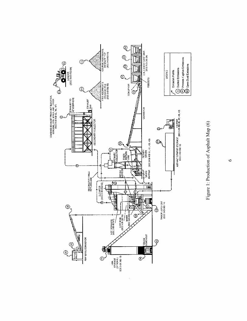
1.3.1. Production of Asphalt Mix

Asphalt mixing can be done one of two ways, either at a drum plant or a batch plant

(6). In either case, the mineral aggregates are heated to a temperature between 135ºC and

180ºC. In a batch mix plant, the aggregates are heated and dried first and then transferred

to a pug mill to be mixed with liquid asphalt. In a drum mix plant, the aggregate is

placed in a dryer that also serves as a mixer to blend with the liquid asphalt. After

mixing, the Hot Mix Asphalt (HMA) is sometimes transferred into a storage tank to be

temporarily stored until paving. These processes can be seen in Figure 1. When the road

is ready to be paved, the HMA is transported by trucks to the project site.

When the HMA is placed onto the road, it is usually done by crews of five to nine

people (6). The HMA remains at a high temperature, of up to 200°C, all the way to the

paving site.

1.3.2 Emissions Produced during Construction

Although not hazardous to humans, asphalt lets off many hazardous emissions,

especially carbon dioxide (CO2), carbon monoxide (CO), and hydrocarbons (6). Another

form of emissions that are dangerous to our atmosphere is Blue smoke, a visible aerosol

emission formed from condensed hydrocarbons. Blue smoke is capable of traveling long

distances before dissipating sufficiently to become invisible. It is an industry-wide

concern for several reasons. These include regulatory limitations, organized opposition,

community concerns, and control equipment requirements.

One form in which greenhouse gas emissions are let off is through the road

construction industry, primarily in the production and laying of asphalt (6). In production

5

of asphalt, the materials need to be heated to increase viscosity of the asphalt to create a

homogeneous mix and to increase workability to effectively place onto the road. Each of

these processes results in high temperatures; traditionally asphalt is heated to a

temperature of 177ºC, resulting in a high level of emissions.

6

Figure 1: Production of Asphalt Map (6)

7

1.4 Additives to Reduce Mix Temperature

Greenhouse gas emissions produced during the construction of asphalt pavements

have led to a need to develop a way to control emissions. In recent years, several

additives have been formulated that claim to maintain a low viscosity at a lower

temperature than conventional asphalt mix without affecting the quality of the pavement

(1). Since the temperature is lower, there is the possibility of reducing greenhouse gas

emissions released during production. These additives could take the industry to a more

environmentally cautious future.

1.4.1 Sasobit®

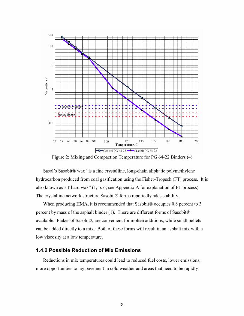
One promising chemical additive that will reduce the temperature needed for an

asphalt mix to have a low viscosity is called Sasobit®, a wax manufactured by Sasol (1).

Sasobit®’s characteristics have led it to be described as an “asphalt flow improver” while

it has been proven to reduce temperatures of asphalt mixes by 18-54ºC (1, p. 7). Figure

2 illustrates an asphalt mix’s decreased viscosity at a lower than conventional

temperature. This additive congeals at an approximate temperature of 102ºC and at

temperatures higher than 120ºC, is completely soluble.

8

Figure 2: Mixing and Compaction Temperature for PG 64-22 Binders (4)

Sasol’s Sasobit® wax “is a fine crystalline, long-chain aliphatic polymethylene

hydrocarbon produced from coal gasification using the Fisher-Tropsch (FT) process. It is

also known as FT hard wax” (1, p. 6; see Appendix A for explanation of FT process).

The crystalline network structure Sasobit® forms reportedly adds stability.

When producing HMA, it is recommended that Sasobit® occupies 0.8 percent to 3

percent by mass of the asphalt binder (1). There are different forms of Sasobit®

available. Flakes of Sasobit® are convenient for molten additions, while small pellets

can be added directly to a mix. Both of these forms will result in an asphalt mix with a

low viscosity at a low temperature.

1.4.2 Possible Reduction of Mix Emissions

Reductions in mix temperatures could lead to reduced fuel costs, lower emissions,

more opportunities to lay pavement in cold weather and areas that need to be rapidly

9

open to traffic (1). Lower asphalt mix temperatures means a reduction in both visible and

non-visible emissions that contribute greenhouse gas emissions.

Carbon dioxide (CO2 ) is the most common and harmful greenhouse gas emission (2).

“It is claimed that CO2 emissions in manufacture are reduced by a factor of 2 for every

10ºC reduction in temperature” (7, p. 1). The rate of oxidation of HMA doubles for every

25ºF (13.9ºC) increase over 200ºF (93.3ºC; 5). A chemical reaction occurs when a

substance combines with oxygen, known as oxidation. As the upper mix surface

oxidizes, carbon dioxide forms. Therefore, lowering the temperature of the mix will in

turn lower the carbon dioxide formed and released to the atmosphere. HMA that is

produced at a lower temperature (using an additive such as Sasobit®) is known as Warm

Mix Asphalt, or WMA (7).

1.5 Objectives

The objectives of this study were to determine if emissions can be reduced with

the use of WMA, and whether any material properties can be expected to improve in

mixes produced at lower temperatures (WMA versus HMA). Another objective was to

determine economic benefits, if any, of producing mixes at lower temperatures.

10

Chapter 2: Scope of Work

The following hypotheses were made:

• In WMA produced at 130°C, Carbon Dioxide, Carbon Monoxide and

Hydrocarbon emissions would be less than emissions released for HMA at a

typical temperature (150°C);

• WMA produced at lower than conventional temperature (130°C) would have

better or equal material properties when compared to HMA produced at a typical

temperature (150°C);

• Using WMA at a lower than conventional temperature (130°C) would lead to

economic benefits. The benefits include cost savings in purchasing asphalt, fuel

needed to heat asphalt and aggregates to high temperatures (150°C) for mixing,

and emission control for asphalt plants.

2.1 Testing Procedures

Testing for this study included emission testing for pure asphalt and asphalt

mixes. HMA (Hot Mix Asphalt) and WMA (Warm Mix Asphalt) samples were also

mixed and compacted to test material properties. All tests completed were done on 3

separate mixes: HMA with 5.3% asphalt, WMA with 5.3% asphalt and 1% Sasobit® (by

mass of asphalt), and WMA with 4.8% asphalt and 1% Sasobit® (by mass of asphalt). A

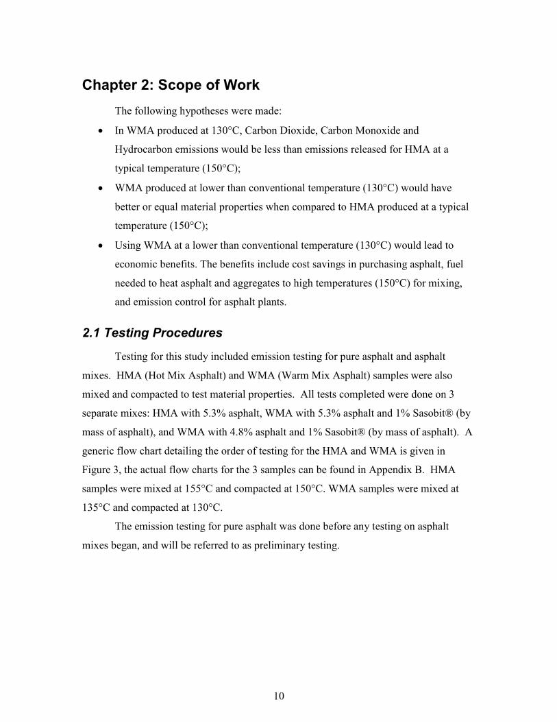
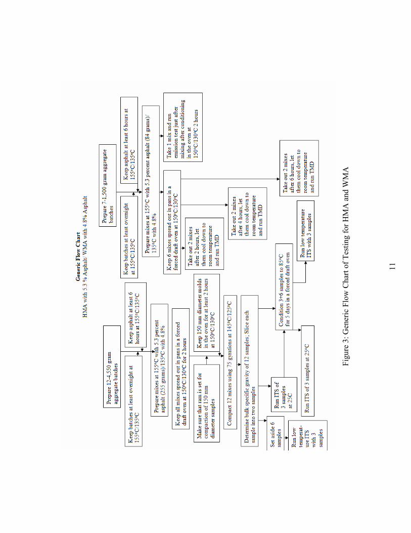
generic flow chart detailing the order of testing for the HMA and WMA is given in

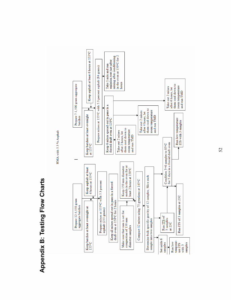
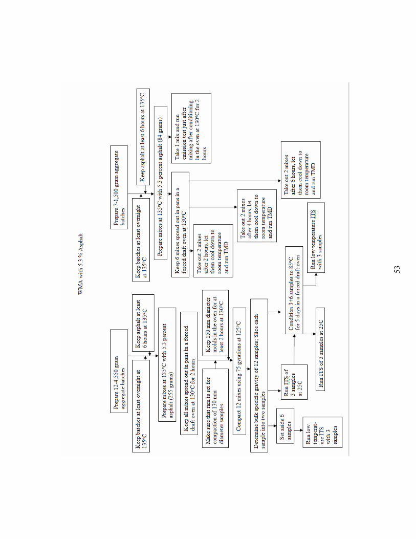
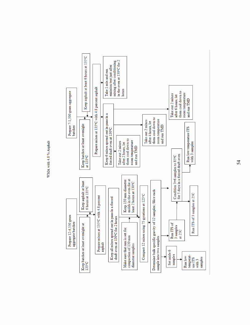
Figure 3, the actual flow charts for the 3 samples can be found in Appendix B. HMA

samples were mixed at 155°C and compacted at 150°C. WMA samples were mixed at

135°C and compacted at 130°C.

The emission testing for pure asphalt was done before any testing on asphalt

mixes began, and will be referred to as preliminary testing.

11

Figure 3: Generic Flow Chart of Testing for HMA and WMA

12

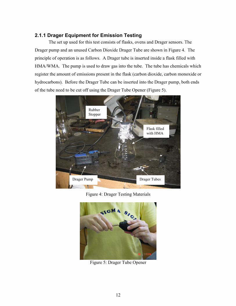
2.1.1 Drager Equipment for Emission Testing

The set up used for this test consists of flasks, ovens and Drager sensors. The

Drager pump and an unused Carbon Dioxide Drager Tube are shown in Figure 4. The

principle of operation is as follows. A Drager tube is inserted inside a flask filled with

HMA/WMA. The pump is used to draw gas into the tube. The tube has chemicals which

register the amount of emissions present in the flask (carbon dioxide, carbon monoxide or

hydrocarbons). Before the Drager Tube can be inserted into the Drager pump, both ends

of the tube need to be cut off using the Drager Tube Opener (Figure 5).

Figure 4: Drager Testing Materials

Figure 5: Drager Tube Opener

Drager Pump Drager Tubes

Flask filled

with HMA

Rubber

Stopper

13

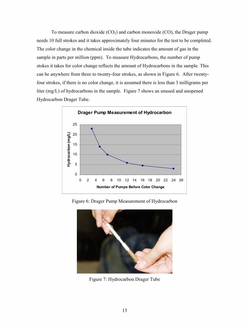
To measure carbon dioxide (CO2) and carbon monoxide (CO), the Drager pump

needs 10 full strokes and it takes approximately four minutes for the test to be completed.

The color change in the chemical inside the tube indicates the amount of gas in the

sample in parts per million (ppm). To measure Hydrocarbons, the number of pump

stokes it takes for color change reflects the amount of Hydrocarbons in the sample. This

can be anywhere from three to twenty-four strokes, as shown in Figure 6. After twenty-

four strokes, if there is no color change, it is assumed there is less than 3 milligrams per

liter (mg/L) of hydrocarbons in the sample. Figure 7 shows an unused and unopened

Hydrocarbon Drager Tube.

Drager Pump Measurement of Hydrocarbon

0

5

10

15

20

25

0 2 4 6 8 10 12 14 16 18 20 22 24 26

Number of Pumps Before Color Change

Hydrocarbon (mg/L)

Figure 6: Drager Pump Measurement of Hydrocarbon

Figure 7: Hydrocarbon Drager Tube

14

2.1.2 Preliminary Testing Procedures

Preliminary testing was completed to determine the best way to collect data on

emissions from asphalt and asphalt mixes since there is not standard procedure. An

empty flask was used as a control test to determine the amount, if any, of emissions

currently in the air. The individual materials asphalt and aggregates were heated

separately in covered containers to our desired temperature in the oven. A mixer was

used to mix the asphalt mix, and the asphalt mix contained approximately 5% asphalt.

After the asphalt and aggregate materials were mixed, they were quickly

transferred into a flask. They were poured into the flask using a tin funnel, and the flask

was capped with tinfoil immediately. The material sat in a covered flask for 15 minutes

to allow enough time to off-gas.

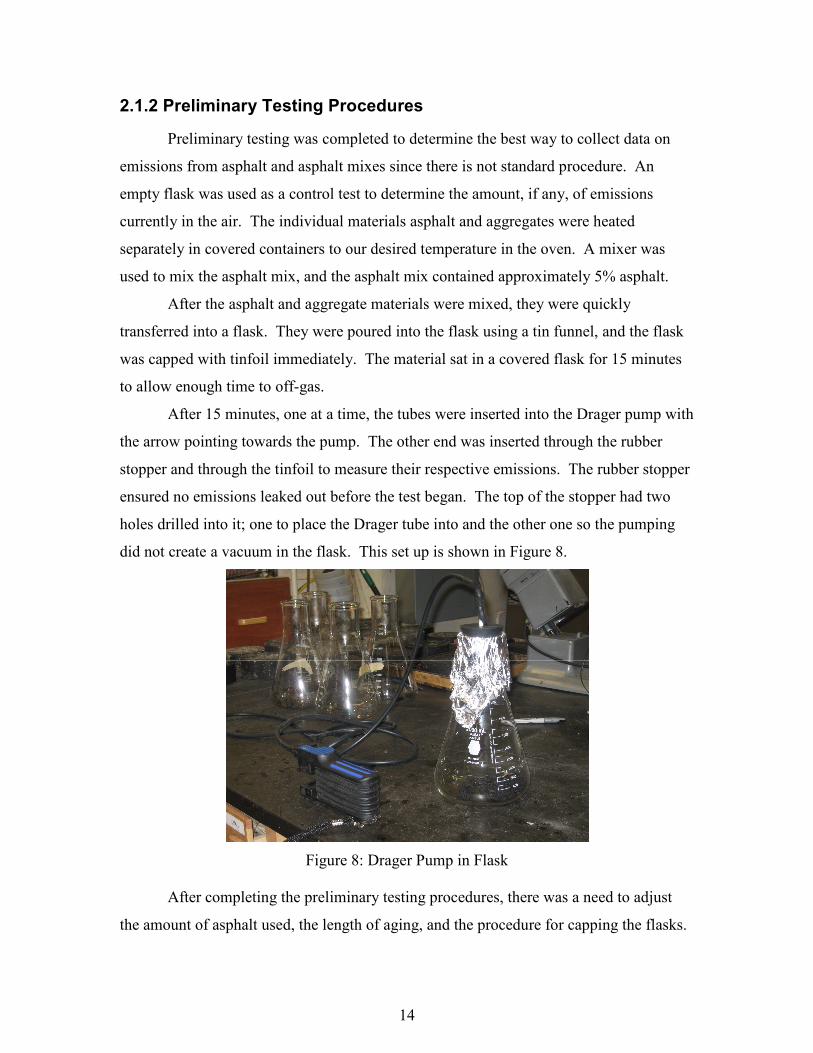
After 15 minutes, one at a time, the tubes were inserted into the Drager pump with

the arrow pointing towards the pump. The other end was inserted through the rubber

stopper and through the tinfoil to measure their respective emissions. The rubber stopper

ensured no emissions leaked out before the test began. The top of the stopper had two

holes drilled into it; one to place the Drager tube into and the other one so the pumping

did not create a vacuum in the flask. This set up is shown in Figure 8.

Figure 8: Drager Pump in Flask

After completing the preliminary testing procedures, there was a need to adjust

the amount of asphalt used, the length of aging, and the procedure for capping the flasks.

15

The amount of asphalt used was a property that had to be tested and readjusted before

determining an amount that provided readable results from the Drager tubes.

After numerous tests with pure asphalt, it was determined that readable results

could only be obtained for carbon dioxide (CO2) if 25-30 grams of pure asphalt were

tested. The carbon monoxide (CO) and hydrocarbon emissions were repeatedly too great

for the Drager tube to read. It was finally determined that the best results would be

obtained using an asphalt mix, as opposed to only pure asphalt. The length of aging was

adjusted to two hours, and the flask was placed back into the oven for those two hours.

The two hours gives the sample adequate time to fill the head space with emissions

before testing. This more closely replicates the actual process used in the field for asphalt

mixing.

2.1.3 Mixing and Compacting

This study analyzed three different asphalt mixes: HMA with 5.3% asphalt,

WMA with 5.3% asphalt and 1% Sasobit® (by mass of asphalt), and WMA with 4.8%

asphalt and 1% Sasobit® (by mass of asphalt). In total, thirty-six samples were

compacted, twelve samples for each of the three mixes. The compacted samples were

made with the 4,550 gram aggregate batches. The mixes used for emission testing and

Theoretical Maximum Density (TMD) testing were made with the 1,500 gram aggregate

batches. Before mixing or compacting could take place, aggregates were sieved to create

36 4,550 gram batches and 24 1,500 gram batches, from washed and dried aggregates

received from All States Asphalt. The PG 64-28 grade asphalt binder was obtained from

the Maine Department of Transportation (MDOT).

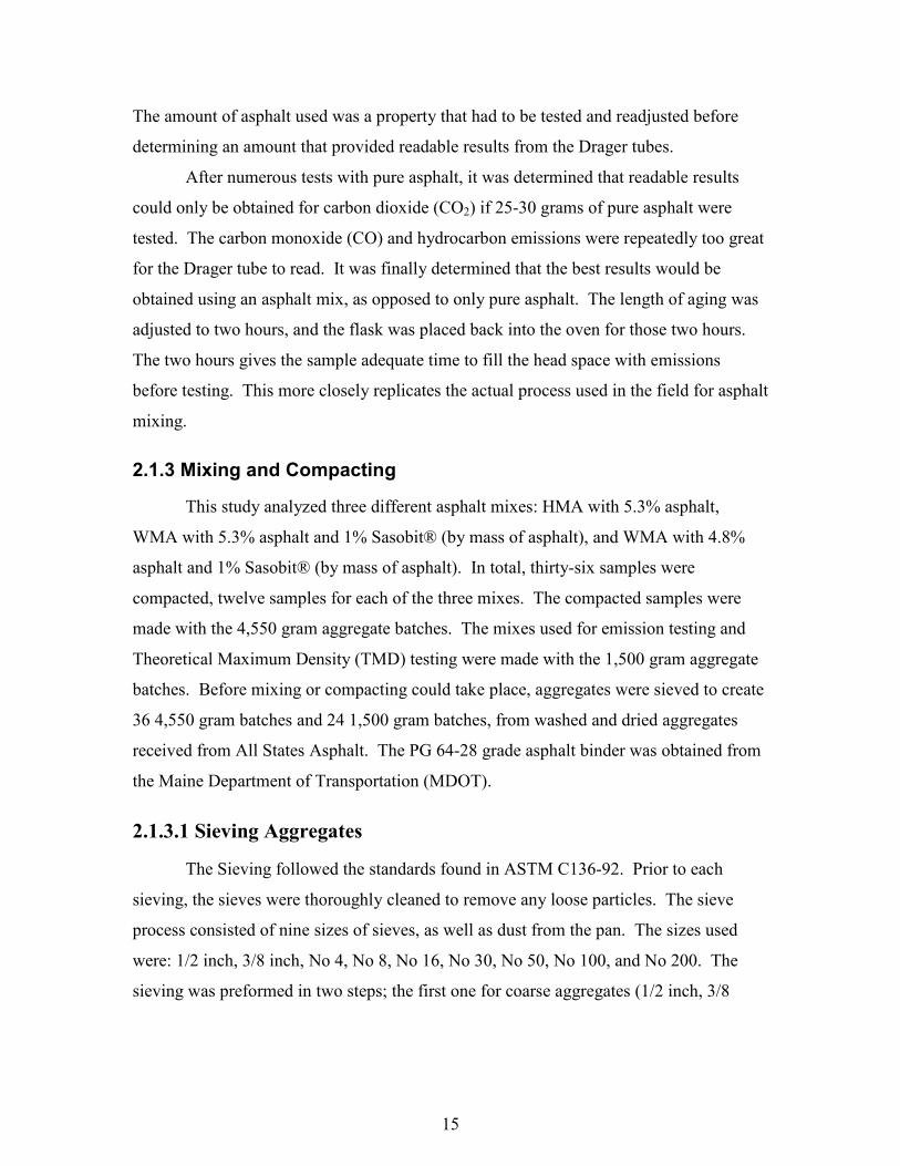
2.1.3.1 Sieving Aggregates

The Sieving followed the standards found in ASTM C136-92. Prior to each

sieving, the sieves were thoroughly cleaned to remove any loose particles. The sieve

process consisted of nine sizes of sieves, as well as dust from the pan. The sizes used

were: 1/2 inch, 3/8 inch, No 4, No 8, No 16, No 30, No 50, No 100, and No 200. The

sieving was preformed in two steps; the first one for coarse aggregates (1/2 inch, 3/8

16

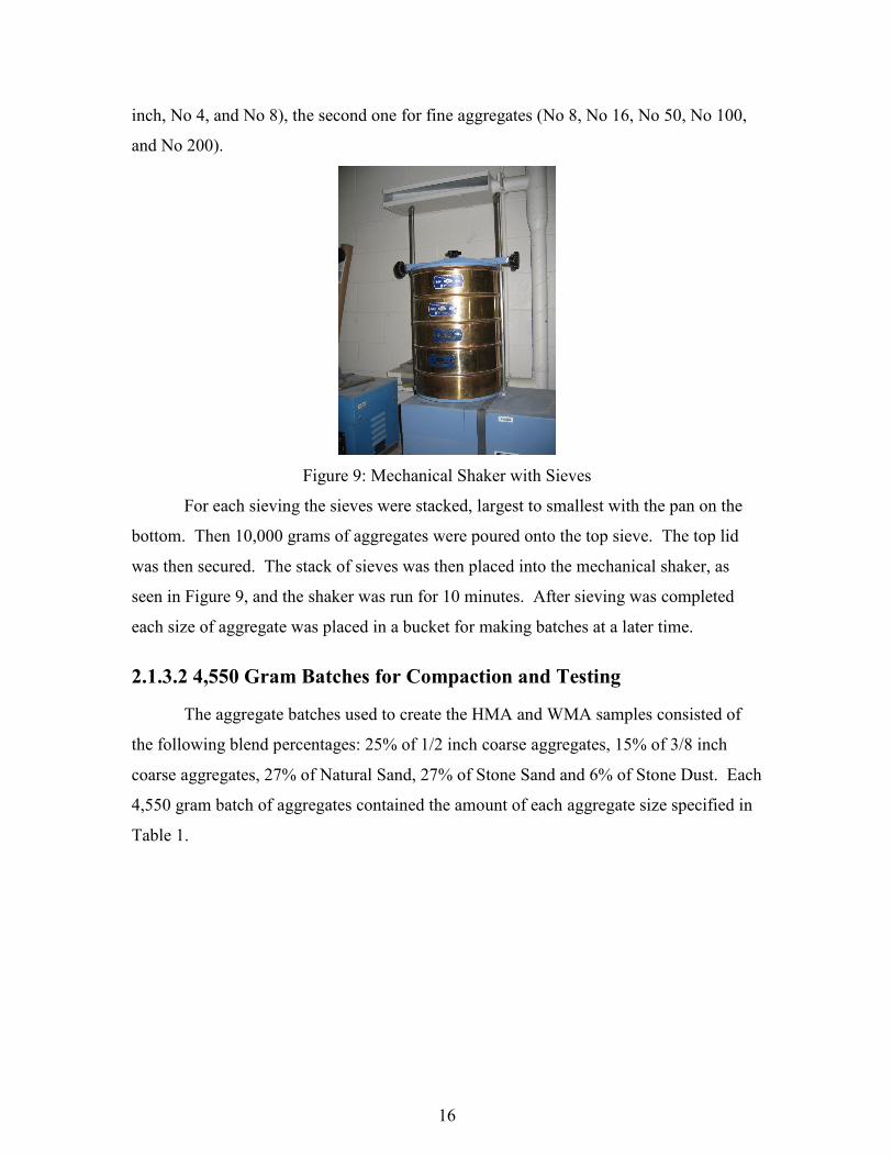
inch, No 4, and No 8), the second one for fine aggregates (No 8, No 16, No 50, No 100,

and No 200).

Figure 9: Mechanical Shaker with Sieves

For each sieving the sieves were stacked, largest to smallest with the pan on the

bottom. Then 10,000 grams of aggregates were poured onto the top sieve. The top lid

was then secured. The stack of sieves was then placed into the mechanical shaker, as

seen in Figure 9, and the shaker was run for 10 minutes. After sieving was completed

each size of aggregate was placed in a bucket for making batches at a later time.

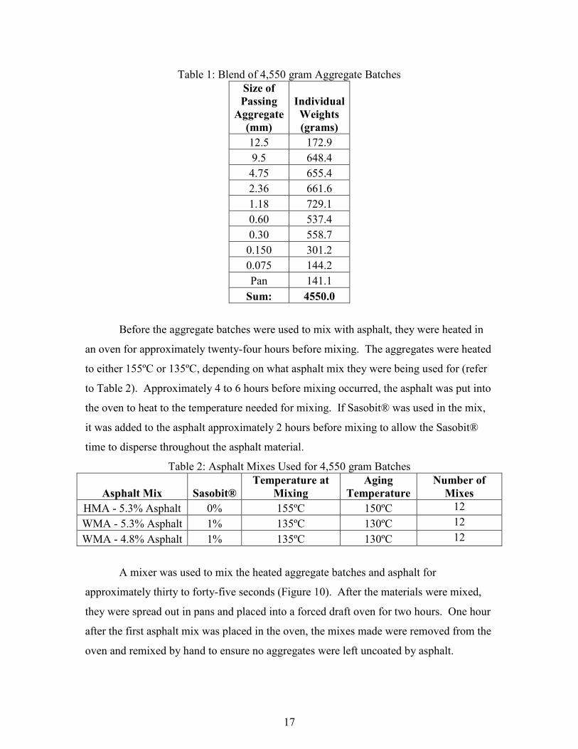
2.1.3.2 4,550 Gram Batches for Compaction and Testing

The aggregate batches used to create the HMA and WMA samples consisted of

the following blend percentages: 25% of 1/2 inch coarse aggregates, 15% of 3/8 inch

coarse aggregates, 27% of Natural Sand, 27% of Stone Sand and 6% of Stone Dust. Each

4,550 gram batch of aggregates contained the amount of each aggregate size specified in

Table 1.

17

Table 1: Blend of 4,550 gram Aggregate Batches

Size of

Passing

Aggregate

(mm)

Individual

Weights

(grams)

12.5 172.9

9.5 648.4

4.75 655.4

2.36 661.6

1.18 729.1

0.60 537.4

0.30 558.7

0.150 301.2

0.075 144.2

Pan 141.1

Sum: 4550.0

Before the aggregate batches were used to mix with asphalt, they were heated in

an oven for approximately twenty-four hours before mixing. The aggregates were heated

to either 155ºC or 135ºC, depending on what asphalt mix they were being used for (refer

to Table 2). Approximately 4 to 6 hours before mixing occurred, the asphalt was put into

the oven to heat to the temperature needed for mixing. If Sasobit® was used in the mix,

it was added to the asphalt approximately 2 hours before mixing to allow the Sasobit®

time to disperse throughout the asphalt material.

Table 2: Asphalt Mixes Used for 4,550 gram Batches

Asphalt Mix Sasobit®

Temperature at

Mixing

Aging

Temperature

Number of

Mixes

HMA - 5.3% Asphalt 0% 155ºC 150ºC 12

WMA - 5.3% Asphalt 1% 135ºC 130ºC 12

WMA - 4.8% Asphalt 1% 135ºC 130ºC 12

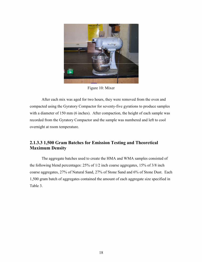
A mixer was used to mix the heated aggregate batches and asphalt for

approximately thirty to forty-five seconds (Figure 10). After the materials were mixed,

they were spread out in pans and placed into a forced draft oven for two hours. One hour

after the first asphalt mix was placed in the oven, the mixes made were removed from the

oven and remixed by hand to ensure no aggregates were left uncoated by asphalt.

18

Figure 10: Mixer

After each mix was aged for two hours, they were removed from the oven and

compacted using the Gyratory Compactor for seventy-five gyrations to produce samples

with a diameter of 150 mm (6 inches). After compaction, the height of each sample was

recorded from the Gyratory Compactor and the sample was numbered and left to cool

overnight at room temperature.

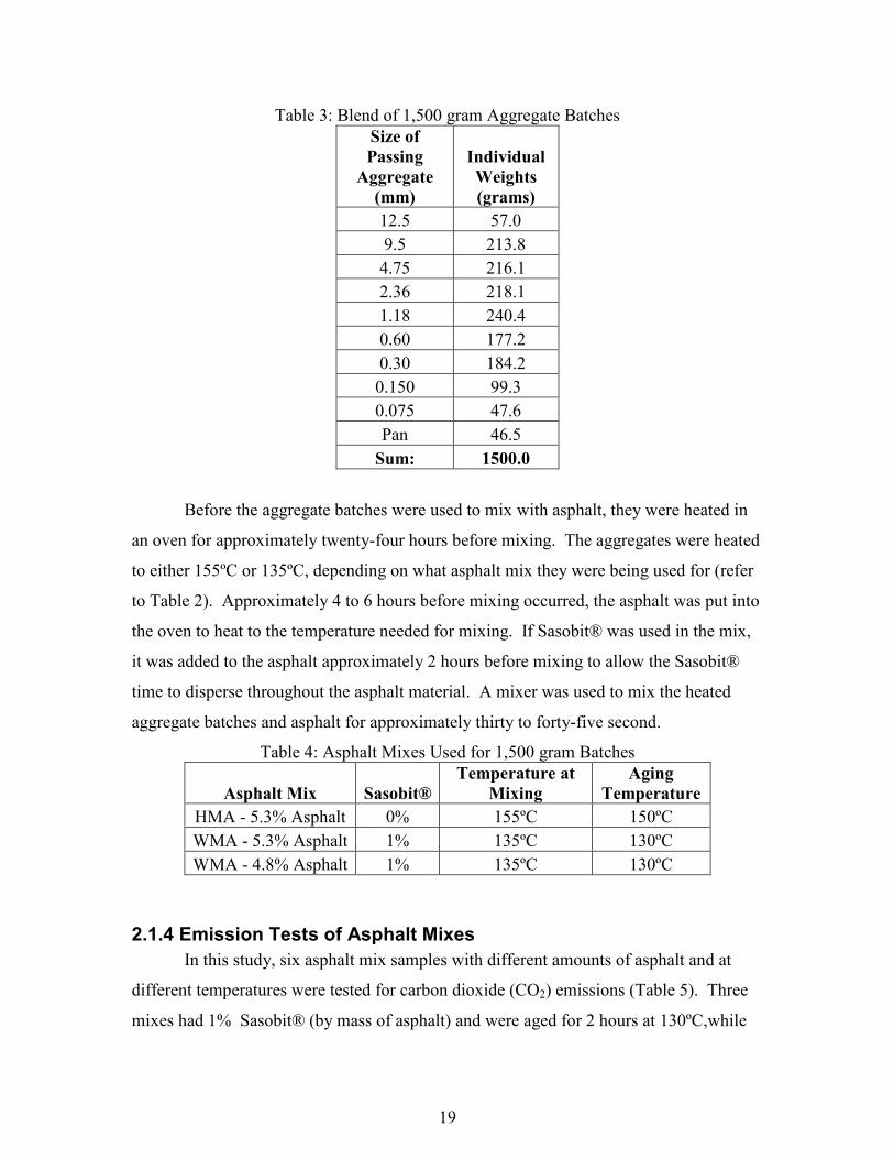
2.1.3.3 1,500 Gram Batches for Emission Testing and Theoretical

Maximum Density

The aggregate batches used to create the HMA and WMA samples consisted of

the following blend percentages: 25% of 1/2 inch coarse aggregates, 15% of 3/8 inch

coarse aggregates, 27% of Natural Sand, 27% of Stone Sand and 6% of Stone Dust. Each

1,500 gram batch of aggregates contained the amount of each aggregate size specified in

Table 3.

19

Table 3: Blend of 1,500 gram Aggregate Batches

Size of

Passing

Aggregate

(mm)

Individual

Weights

(grams)

12.5 57.0

9.5 213.8

4.75 216.1

2.36 218.1

1.18 240.4

0.60 177.2

0.30 184.2

0.150 99.3

0.075 47.6

Pan 46.5

Sum: 1500.0

Before the aggregate batches were used to mix with asphalt, they were heated in

an oven for approximately twenty-four hours before mixing. The aggregates were heated

to either 155ºC or 135ºC, depending on what asphalt mix they were being used for (refer

to Table 2). Approximately 4 to 6 hours before mixing occurred, the asphalt was put into

the oven to heat to the temperature needed for mixing. If Sasobit® was used in the mix,

it was added to the asphalt approximately 2 hours before mixing to allow the Sasobit®

time to disperse throughout the asphalt material. A mixer was used to mix the heated

aggregate batches and asphalt for approximately thirty to forty-five second.

Table 4: Asphalt Mixes Used for 1,500 gram Batches

Asphalt Mix Sasobit®

Temperature at

Mixing

Aging

Temperature

HMA - 5.3% Asphalt 0% 155ºC 150ºC

WMA - 5.3% Asphalt 1% 135ºC 130ºC

WMA - 4.8% Asphalt 1% 135ºC 130ºC

2.1.4 Emission Tests of Asphalt Mixes

In this study, six asphalt mix samples with different amounts of asphalt and at

different temperatures were tested for carbon dioxide (CO2) emissions (Table 5). Three

mixes had 1% Sasobit® (by mass of asphalt) and were aged for 2 hours at 130ºC,while

20

the other three mixes contained no Sasobit® and were aged for 2 hours at 150ºC.

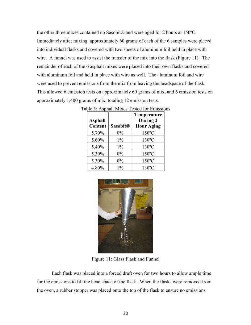
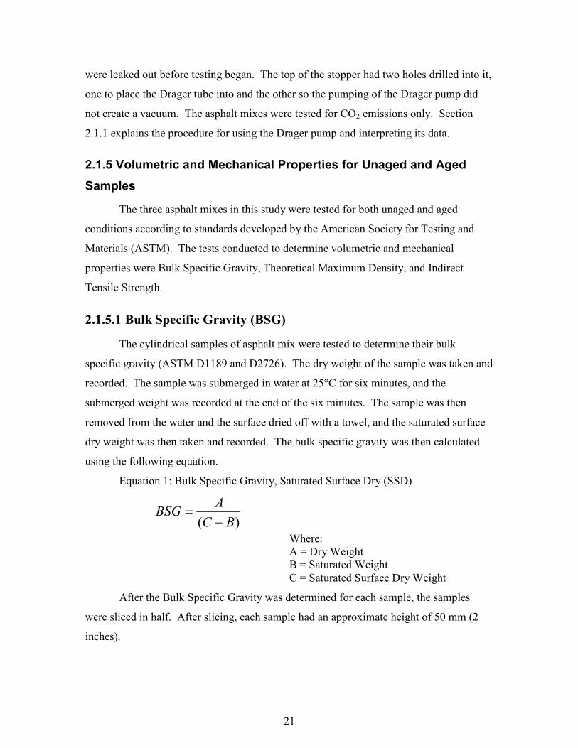
Immediately after mixing, approximately 60 grams of each of the 6 samples were placed

into individual flasks and covered with two sheets of aluminum foil held in place with

wire. A funnel was used to assist the transfer of the mix into the flask (Figure 11). The

remainder of each of the 6 asphalt mixes were placed into their own flasks and covered

with aluminum foil and held in place with wire as well. The aluminum foil and wire

were used to prevent emissions from the mix from leaving the headspace of the flask.

This allowed 6 emission tests on approximately 60 grams of mix, and 6 emission tests on

approximately 1,400 grams of mix, totaling 12 emission tests.

Table 5: Asphalt Mixes Tested for Emissions

Asphalt

Content Sasobit®

Temperature

During 2

Hour Aging

5.70% 0% 150ºC

5.60% 1% 130ºC

5.40% 1% 130ºC

5.30% 0% 150ºC

5.30% 0% 150ºC

4.80% 1% 130ºC

Figure 11: Glass Flask and Funnel

Each flask was placed into a forced draft oven for two hours to allow ample time

for the emissions to fill the head space of the flask. When the flasks were removed from

the oven, a rubber stopper was placed onto the top of the flask to ensure no emissions

21

were leaked out before testing began. The top of the stopper had two holes drilled into it,

one to place the Drager tube into and the other so the pumping of the Drager pump did

not create a vacuum. The asphalt mixes were tested for CO2 emissions only. Section

2.1.1 explains the procedure for using the Drager pump and interpreting its data.

2.1.5 Volumetric and Mechanical Properties for Unaged and Aged

Samples

The three asphalt mixes in this study were tested for both unaged and aged

conditions according to standards developed by the American Society for Testing and

Materials (ASTM). The tests conducted to determine volumetric and mechanical

properties were Bulk Specific Gravity, Theoretical Maximum Density, and Indirect

Tensile Strength.

2.1.5.1 Bulk Specific Gravity (BSG)

The cylindrical samples of asphalt mix were tested to determine their bulk

specific gravity (ASTM D1189 and D2726). The dry weight of the sample was taken and

recorded. The sample was submerged in water at 25°C for six minutes, and the

submerged weight was recorded at the end of the six minutes. The sample was then

removed from the water and the surface dried off with a towel, and the saturated surface

dry weight was then taken and recorded. The bulk specific gravity was then calculated

using the following equation.

Equation 1: Bulk Specific Gravity, Saturated Surface Dry (SSD)

)( BC

ABSG

−=

Where: A = Dry Weight

B = Saturated Weight C = Saturated Surface Dry Weight

After the Bulk Specific Gravity was determined for each sample, the samples

were sliced in half. After slicing, each sample had an approximate height of 50 mm (2

inches).

22

2.1.5.2 Theoretical Maximum Density (TMD)

The Theoretical Maximum Density was measured using ASTM D2041. Samples

of Asphalt Mix were mixed according to the procedure in Section 2.1.2.3 to create 1,500

gram batches. Each mix was broken up while still hot after mixing, separating the

aggregates as much as possible. The separated sample was then spread out into pan and

aged in a forced draft oven for either two, four or six hours at the desired temperature.

The HMA was aged at 150°C and the WMA was aged at 130°C. The different periods of

aging were used to determine the increase in absorption with time of aging, if any.

When the samples were removed from the oven, they were allowed to cool down

to room temperature. At room temperature, an empty bowl was weighed in air and while

submerged in water, and recorded. The separated mix was then placed into the empty

bowl and the weight of the bowl and the mix was recorded in air. The bowl was then

filled with water to a height of approximately one inch above the mix. The bowl was

placed into the Gilson Vibro-Deairator and the lid was secured in place. Then the

vacuum pump was turned on until the air pressure inside the bowl reached 27 Hg. At that

point, the Deairator was turned on and allowed to run for ten minutes. After ten minutes,

the Deairator and vacuum pump were turned off and the valve was slowly released to

remove the pressure inside the bowl. Then without disturbing the mix, the bowl with the

aggregates was submerged into water at 25°C. After ten minutes, the submerged weight

was recorded. The Theoretical Maximum Density of the mix was calculated using the

following equation.

Equation 2: Theoretical Maximum Density, TMD

( )( ) ( )[ ]DBCA

CATMD

−−−−

=

Where: A = Sample weight in Air (with bowl) B = Sample weight in H20 (with bowl) C = Weight of bowl in Air D = Weight of bowl in H20

The BSG and TMD, along with the specific gravities of the aggregates and

asphalt (known), allowed the determination of percentage of asphalt absorbed and the

effective asphalt content in the mix.

23

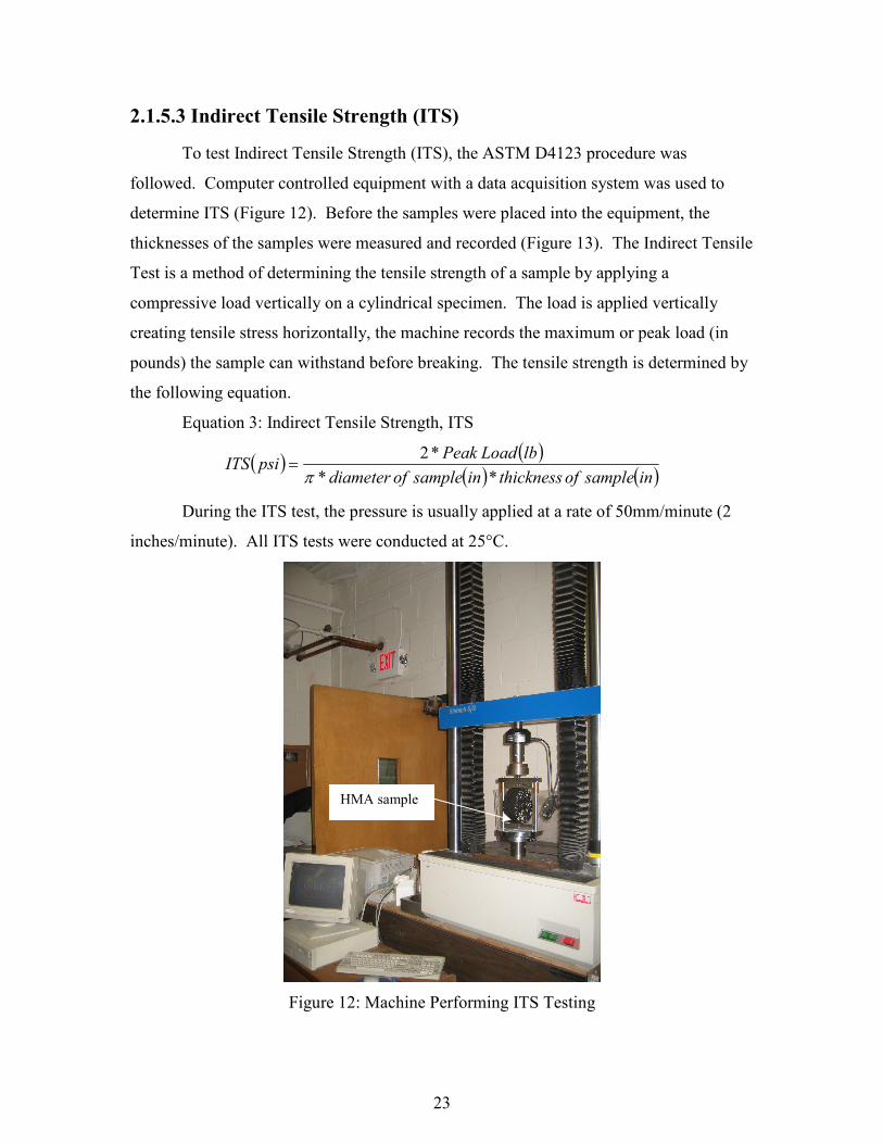
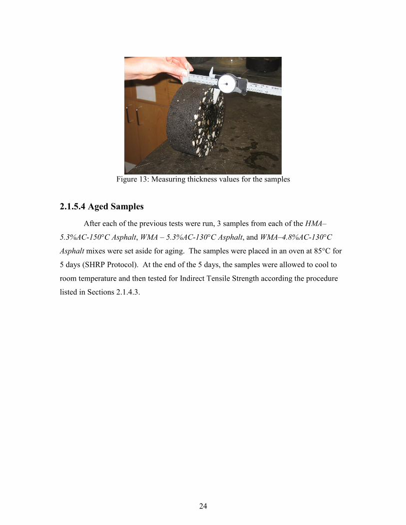
2.1.5.3 Indirect Tensile Strength (ITS)

To test Indirect Tensile Strength (ITS), the ASTM D4123 procedure was

followed. Computer controlled equipment with a data acquisition system was used to

determine ITS (Figure 12). Before the samples were placed into the equipment, the

thicknesses of the samples were measured and recorded (Figure 13). The Indirect Tensile

Test is a method of determining the tensile strength of a sample by applying a

compressive load vertically on a cylindrical specimen. The load is applied vertically

creating tensile stress horizontally, the machine records the maximum or peak load (in

pounds) the sample can withstand before breaking. The tensile strength is determined by

the following equation.

Equation 3: Indirect Tensile Strength, ITS

( ) ( )( ) ( )insampleofthicknessinsampleofdiameter

lbLoadPeakpsiITS

**

*2

π=

During the ITS test, the pressure is usually applied at a rate of 50mm/minute (2

inches/minute). All ITS tests were conducted at 25°C.

Figure 12: Machine Performing ITS Testing

HMA sample

24

Figure 13: Measuring thickness values for the samples

2.1.5.4 Aged Samples

After each of the previous tests were run, 3 samples from each of the HMA–

5.3%AC-150°C Asphalt, WMA – 5.3%AC-130°C Asphalt, and WMA–4.8%AC-130°C

Asphalt mixes were set aside for aging. The samples were placed in an oven at 85°C for

5 days (SHRP Protocol). At the end of the 5 days, the samples were allowed to cool to

room temperature and then tested for Indirect Tensile Strength according the procedure

listed in Sections 2.1.4.3.

25

Chapter 3: Results

The results of this study are organized into three sections: Volumetric Properties,

Emissions and Mechanical Properties. The volumetric property results discuss percent

air voids, absorption and effective asphalt content. The emission results show measured

emissions from both pure asphalt and asphalt mixes. The mechanical property results

discuss Indirect Tensile Strength of both aged and unaged samples.

3.1 Volumetric Properties

The volumetric properties of the three different asphalt mixes calculated were

percent air voids, absorption, and effective asphalt content. With the values of bulk

specific gravity and theoretical maximum density, percent air voids could be calculated.

This allowed the comparison of absorption and effective asphalt content.

3.1.1. Percent Air Voids

The percent Air Voids for each sample are shown in Table 6 below. Each percent

air void was found after calculating the Bulk Specific Gravity and Theoretical Maximum

Density (results in Section 3.1.2). The value for Theoretical Maximum Density used is

the value calculated after being aged for 2 hours, the standard aging time for Theoretical

Maximum Density. The percent Air Voids are calculated by the following equation.

Equation 4: Percent Air Void

−=TMD

BSGVoidAir

*100100%

Where: BSG = Bulk Specific Gravity TMD = Theoretical Maximum Density

26

Table 6: Bulk Specific Gravity & Percent Air Voids

Mix Sample Dry, g Under Water, g SSD, g BSG Gmm/TMD Air voids Density

HMA-5.3%AC-150C 1 4624 2693 4628.5 2.38905 4.9 95.1

HMA-5.3%AC-150C 2 4723 2741 4724.5 2.38114 5.2 94.8

HMA-5.3%AC-150C 3 4745.5 2762 4748.5 2.38887 4.9 95.1

HMA-5.3%AC-150C 4 4774 2776.5 4779 2.38402 5.1 94.9

HMA-5.3%AC-150C 5 4732.5 2747 4742 2.37218 5.6 94.4

HMA-5.3%AC-150C 6 4721 2743.5 4727 2.38014 5.3 94.7

HMA-5.3%AC-150C 7 4615.5 2689 4619.5 2.39083 4.9 95.1

HMA-5.3%AC-150C 8 4653 2704 4658.5 2.38066 5.3 94.7

HMA-5.3%AC-150C 9 4623.5 2681 4628.5 2.37407 5.5 94.5

HMA-5.3%AC-150C 10 4707.5 2736.5 4711 2.38415 5.1 94.9

HMA-5.3%AC-150C 11 4642 2697 4644 2.38418 5.1 94.9

HMA-5.3%AC-150C 12 4748 2757.5 4753 2.37935

2.513

5.3 94.7

Average 5.2 94.8

WMA-5.3%AC-130C 13-5.3% 4758 2773 4760.5 2.39396 2.491 3.9 96.1

WMA-5.3%AC-130C 14-5.3% 4737 2749 4740 2.37921 4.5 95.5

WMA-5.3%AC-130C 15-5.3% 4779 2784 4782.5 2.39129 4.0 96.0

WMA-5.3%AC-130C 16-5.3% 4722 2753.5 4723.5 2.39695 3.8 96.2

WMA-5.3%AC-130C 17-5.3% 4707.5 2737 4711.5 2.38415 4.3 95.7

WMA-5.3%AC-130C 18-5.3% 4703 2733.5 4706.5 2.38368 4.3 95.7

WMA-5.3%AC-130C 19-5.3% 4749.5 2742.5 4723.5 2.39753 3.8 96.2

WMA-5.3%AC-130C 20-5.3% 4779.5 2791 4782.5 2.39995 3.7 96.3

WMA-5.3%AC-130C 21-5.3% 4671.5 2725 4676 2.39441 3.9 96.1

WMA-5.3%AC-130C 22-5.3% 4702 2759 4699 2.42371 2.7 97.3

WMA-5.3%AC-130C 23-5.3% 4732.5 2781.5 4725.5 2.43441 2.3 97.7

WMA-5.3%AC-130C 24-5.3% 4716 2767 4717 2.41846 2.9 97.1

WMA-5.3%AC-130C 1-4.8% 4663.4 2675.5 4670.5 2.33754 6.2 93.8

Average 3.9 96.1

WMA-4.8%AC-130C 2-4.8% 4757.5 2736.1 4765.1 2.34475 2.51 6.6 93.4

WMA-4.8%AC-130C 3-4.8% 4706.5 2699 4713 2.33689 6.9 93.1

WMA-4.8%AC-130C 4-4.8% 4707.5 2702.5 4717.6 2.33611 6.9 93.1

WMA-4.8%AC-130C 5-4.8% 4705.6 2707.5 4715.2 2.34378 6.6 93.4

WMA-4.8%AC-130C 6-4.8% 4647.9 2669.1 4654.4 2.34116 6.7 93.3

WMA-4.8%AC-130C 7-4.8% 4707 2719.2 4712 2.362 5.9 94.1

WMA-4.8%AC-130C 8-4.8% 4632.4 2660.5 4637.7 2.34291 6.7 93.3

WMA-4.8%AC-130C 9-4.8% 4659.1 2684.5 4667.2 2.34988 6.4 93.6

WMA-4.8%AC-130C 10-4.8% 4672.9 2698.1 4682.2 2.35517 6.2 93.8

WMA-4.8%AC-130C 11-4.8% 4650.5 2678.7 4659.8 2.34743 6.5 93.5

WMA-4.8%AC-130C 12-4.8% 4603.7 2650.2 4613.8 2.34452 6.6 93.4

Average 6.5 93.5

27

As is shown in the table and the chart below, the Asphalt Mix with the highest

amount of Air Voids is the WMA-4.8%AC-130ºC. As asphalt content decreases it is

natural for the Percent Air Voids to increase in a sample. This does not mean that using

4.8% asphalt instead of 5.3% asphalt is worse for a given asphalt mix. Instead, the

sample needs to be compacted more to eliminate air voids. Asphalt mixes with a smaller

percent asphalt content need to be compacted more.

However, the more important thing is that the use of Sasobit® at a lower

temperature of 130ºC (20ºC lower than 150ºC) produced a higher density with the same

compaction effort. A higher density in an asphalt mix means that there are less air voids.

This higher density should produce asphalt mixes with better mechanical properties, as

well as lower in-place oxidation and aging.

Percent Air Voids

0

1

2

3

4

5

6

7

HMA-5.3%AC-150C WMA-5.3%AC-130C WMA-4.8%AC-130C

Asphalt Mixes

Average Air Voids (%)

Figure 14: Average Air Voids

3.1.2 Absorption & Effective Asphalt Content

The TMD values were used to find the Effective Specific Gravity as shown in the

equation below.

28

Equation 5: Effective Specific Gravity, Gse

−

=

b

b

s

SE

G

P

TMD

PG

100

Where: Ps = Percent Stone Pb = Percent Binder TMD = Theoretical Maximum Density Gb = Specific Gravity of Binder

(assumed to be 1.03)

Then the Bulk Volume of Stone and Effective Volume of Stone are calculated

using the following equations.

Equation 6: Bulk Volume of Stone, Vsb

( )sb

b

sbG

PV

−=100

Where: Vsb = Bulk Volume of Stone Pb = Percent Binder Gsb = Bulk Specific Gravity = 2.627

Equation 7: Effective Volume of Stone, Vse

( )se

b

seG

PV

−=100

Where: Vsb = Effective Volume of Stone Pb = Percent Binder Gse = Effective Specfic Gravity

Then the Absorbed Asphalt Content can be calculated by subtracting the Effective

Volume of Stone from the Bulk Volume of Stone. Finally, an Effective Asphalt Content

can be calculated by subtracting the Absorbed Asphalt Content from the Total Volume of

Asphalt for a given mix of 100 grams. These results are shown in Table 7.

ContentAsphaltAbosorbedAsphaltofVolumeTotalContentAsphaltEffective −=

29

Table 7: Volume of Effective Asphalt

Mix

Temperature,

Mixing and

Aging, C

Aging

Period,

hours

TMD

Pb

Ps

Gse

Total volume

of asphalt

(Consider

100gm of mix)

Gsb

Vsb,cc Vse,cc Absorbed

AC, cc

Volume

of

Effective

Asphalt,

cc

HMA-5.3%AC-150C

150

2

2.513

5.3 94.7 2.733

5.146

2.627 36.049 34.647

1.401

3.744

HMA-5.3%AC-150C

150

4

2.535

5.3 94.7 2.761

5.146

2.627 36.049 34.302

1.747

3.399

HMA-5.3%AC-150C

150

6

2.519

5.3 94.7 2.741

5.146

2.627 36.049 34.553

1.496

3.650

WMA-5.3%AC-130C

125

2

2.491

5.3 94.7 2.706

5.146

2.627 36.049 34.999

1.050

4.096

WMA-5.3%AC-130C

125

4

2.502

5.3 94.7 2.720

5.146

2.627 36.049 34.822

1.226

3.919

WMA-5.3%AC-130C

125

6

2.505

5.3 94.7 2.723

5.146

2.627 36.049 34.775

1.274

3.871

WMA-4.8%AC-130C

125

2

2.51

4.8 95.2 2.706

4.660

2.627 36.239 35.180

1.059

3.602

WMA-4.8%AC-130C

125

4

2.511

4.8 95.2 2.707

4.660

2.627 36.239 35.165

1.074

3.586

WMA-4.8%AC-130C

125

6

2.515

4.8 95.2 2.712

4.660

2.627 36.239 35.101

1.138

3.522

30

As the table above shows, the Volume of Effective Asphalt was largest for the

WMA – 5.3%AC – 130ºC asphalt mix, and about the same for the other two mixes. Since

the HMA – 5.3% - 150ºC and the WMA – 5.3% - 130ºC both have the same amount of

asphalt; the higher temperature has an effect on the amount of asphalt absorbed by the

stone. This shows that by using the additive Sasobit®, with Warm Mix Asphalt, a lower

absorption and hence a higher effective asphalt content compared to that in the HMA can

be obtained. This high effective asphalt content should mean greater durability of the

mixture.

3.2 Emissions

Greenhouse gas emissions were tested for both pure asphalt and asphalt mixes.

Approximately twenty-five to two hundred grams of pure asphalt was tested for different

lengths of time at different temperatures. The asphalt mixes were tested only for carbon

dioxide with half of the mixes containing Sasobit® and half without, at a range of

temperatures. As testing was completed, the final testing procedure was determined for

this study.

3.2.1 Emissions of Asphalt

There is no standard procedure for measuring emissions produced by asphalt

materials in the laboratory. The procedures used for these tests were found by trial and

error. The mass of asphalt tested and the time allowed for the headspace to fill the

headspace were the most important variables that needed to be determined. Materials

were obtained to measure carbon dioxide (CO2), carbon monoxide (CO) and

hydrocarbons with the Drager pump of the asphalt after a given amount of time.

The first trial (9/27/2006) of emission tests were done after allowing

approximately 199 grams of asphalt to off-gas for 24 hours at 2 temperatures, 130ºC and

160ºC (Table 8). The results for all 3 emissions of the asphalt held at 160ºC were larger

than Drager tubes measured. The CO and hydrocarbon content were also larger than

what Drager tubes could detect for the asphalt held at 130ºC for 24 hours. Although for

the same asphalt at 130 ºC, the CO2 was measured to be 2,500 ppm.

31

Table 8: Pure Asphalt Emissions

The second trial (10/10/2006) of emission tests were done after allowing

approximately 50 grams to off-gas for 24 hours at 120 ºC and 170 ºC (Table 8). The

results for all 3 emissions of the asphalt held at 170ºC were larger than Drager tubes

measured. The emission results for the asphalt held at 120ºC for 24 hours were

obtainable. The CO2 present was measured to be 1,400 ppm, the CO was measured at

200 ppm and the hydrocarbon was found to be 14 mg/L. The lower mass of asphalt, 50

grams instead of 199 grams, was more promising and found results measurable by Drager

products.

The third trial (11/2/2006) of emission tests were done on 23.5 grams of asphalt

after off-gassing for 24 hours at 150ºC. The results for CO2, CO and hydrocarbon were

all immeasurable by Drager products since they were so high. The results for this test

were expected, since the mass of asphalt was decreased by half from approximately 50

grams to 23.5 grams. The higher temperature of 150ºC caused more emissions to be off-

gassed than at 120ºC.

In an attempt to have CO2, CO and hydrocarbon be measurable by the Drager

pump, the time allowed for the asphalt to fill the headspace of the flask was reduced to 2

hours from 24 hours. The fourth trial (11/9/2006) was completed with 30 grams of

Measured Emissions

Hydrocarbons (mg/L)

Date

Asphalt Temperature

(ºC) Time allowed in oven at temperature

Mass of Asphalt (grams)

Carbon Dioxide (ppm)

Carbon Monoxide (ppm)

Number of

strokes mg/L

9/27/2006 130 24 hours 199.1 2500 > 300 4 18.5

9/27/2006 160 24 hours 20 minutes 199 > 3000 > 300 2 > 23

10/10/2006 120 24 hours 50.5 1400 200 5 14

10/10/2006 170 24 hours 20 minutes 50 > 3000 > 300 1 > 23

11/3/2006 150 24 hours 23.5 > 3000 > 300 1 > 23

11/9/2006 150 2 hours 30 800 > 300 1 > 23

11/10/2006 125 2 hours 27.5 600

11/10/2006 150 2 hours 30 800

11/10/2006 170 2 hours 25 1300

Maximum Emissions read by Drager Tube 3000 300 3 23

32

asphalt held at 150ºC for 2 hours. The CO2 present was measured to be 800 ppm, while

the CO and hydrocarbon was still too large for the Drager pump to measure. Because

results for emissions of CO and hydrocarbon could not be measured from asphalt unless

it was at a temperature below 130ºC, the procedure was amended to only measure CO2

emissions. CO2 emissions were most likely to be measured at any temperature ranging

from 120ºC to 150ºC from the tests completed to this point.

The final trial (11/10/2006) measuring CO2 emissions from pure asphalt was done

after holding asphalt at 125ºC, 150ºC and 170ºC for 2 hours. The CO2 measured for 27.5

grams of asphalt at 125ºC was 600 ppm. The CO2 measured for 30 grams of asphalt at

150ºC was found to be 800 ppm and the CO2 measured for 25 grams of asphalt at 170ºC

was 1,300 ppm (Figure 15).

Emissions of Pure Asphalt

0

500

1000

1500

2000

2500

3000

3500

80 90 100 110 120 130 140 150 160 170 180

Temperature of Asphalt during Testing (ºC)

Carbon Dioxide Emissions (ppm)

30g Aged for 2 Hours 200g Aged for 24 Hours 50g Aged for 24 Hours

Figure 15: Carbon Dioxide (CO2) Emissions of Pure Asphalt

From the procedures described on measuring emissions from pure asphalt, the

best combination of mass of asphalt tested and time allowed for the material to off-gas

was chosen. The time chosen for off-gassing was 2 hours, and the desired amount of

pure asphalt to be tested was approximately 30 grams.

33

3.2.2 Emissions of Asphalt Mixes

The procedure developed to test Carbon Dioxide (CO2) emissions from asphalt

mixes was to allow approximately 60 grams of asphalt mix to off-gas for 2 hours. This

was done for 3 mixes with 1% Sasobit® (by mass of asphalt) that off-gassed in an oven

for 2 hours are 130ºC, and 3 mixes without Sasobit® that off-gassed for 2 hours at 150ºC

(Table 9). This asphalt content of the different mixes tested ranged from 4.8% to 5.7%.

Table 9: Carbon Dioxide (CO2) Emissions from Asphalt Mixes

There is a clear difference in the amount of CO2 present in the headspace of the

HMA with Sasobit® at 130ºC and the WMA without Sasobit® at 150ºC. The amount of

CO2 present in the HMA mixes range from 700 ppm to 750 ppm while the amount

present in the WMA range from 450 ppm to 550 ppm.

3.3 Mechanical Properties

The mechanical property of the three different asphalt mixes tested was Indirect

Tensile Strength (ITS). The ITS results showed the most positive impacts of the

Sasobit® additive in the mixes.

3.3.1 Indirect Tensile Strength

The Indirect Tensile Strength values we found are shown in Table 10 below. The

averages for each set of samples were taken and shown in the graph as well. Finally, the

Average change in Tensile Strength after aging was calculated by using the following

equation.

Mix Sasobit®

(%)

Temperature

(ºC) During 2

Hour Aging

Mass of

Mix

(grams)

Asphalt

Content

(%)

Time in

Oven

(hours)

CO2

(ppm)

HMA 0 150 61.2 5.7 2 700

HMA 0 150 59.5 5.3 2 700

HMA 0 150 60.7 5.3 2 750

WMA 1 130 61.3 5.6 2 550

WMA 1 130 62.3 5.4 2 550

WMA 1 130 62.7 4.8 2 450

34

Equation 8: Average Change after Aging

( )StrengthAverageUnaged

StrengthAverageUnagedStrengthAverageAgedAgingAfterChangeAverage

−= *100

Table 10: Indirect Tensile Strength

Mix Condition Sample Thickness,

in Peak Load,

lb

Tensile strength,

psi

Tensile Strength,

kpa

Average change after

aging (+increase)

HMA-5.3%AC-150C Unaged HMA-2a-unaged 2.134 2201.6 343.89 2372.86

HMA-6a-unaged 2.367 3280.7 462.01 3187.84

HMA-8a-unaged 2.207 2496.3 377.03 2601.49

Average 2720.73

Aged HMA-2b-aged 2.134 2999.7 468.56 3233.04

HMA-6a-aged 2.367 3288.2 463.06 3195.12

HMA-8b-aged 2.207 3001.7 453.36 3128.19

Average 3185.45 17.08

WMA-5.3%AC-130C Unaged WMA-22a-unaged 2.06275 2770.9

447.77 3089.60

WMA-24a-unaged 2.056 2775

449.90 3104.33

WMA-15b-unaged 2.20675 2239.2

338.23 2333.82

Average 2842.58

Aged WMA-22a-aged 2.06275 2629.7 424.95 2932.16

WMA-24a-aged 2.056 3280.3 531.83 3669.60

WMA-15b-aged 2.20675 2932.4 442.94 3056.31

Average 3219.36 13.25

WMA-4.8%AC-130C Unaged WMA-3b-unaged 2.40225 2230.9 309.56 2135.94

WMA-5a-unaged 2.2305 2465.9 368.51 2542.73

WMA-6b-unaged 2.2065 1524.9 230.36 1589.52

Average 2089.40

Aged WMA-4a-aged 2.139 3154.5 491.58 3391.94

WMA-7b-aged 2.252 3146.3 465.70 3213.36

WMA-9a-aged 2.213 3047.4 459.01 3167.20

Average 3257.50 55.91

Above, in Table 10, is a summary of the ITS values, density and the average

change in ITS after aging. After analyzing the table, it can be concluded that the most

effective asphalt mix is the WMA-5.3%-AC-130ºC because of the high density and ITS

and the low change after aging. The high density means that the mix will have few air

voids, which make it a more desirable asphalt mix. The mix also has a high tensile

strength unaged and a relatively low change in the strength after aging the sample. This

35

means that in the field the sample will maintain a high strength as the asphalt ages over

time.

36

Chapter 4: Analysis

The Analysis of this study can be separated into three distinct areas: volumetric

properties analysis, asphalt mix emission analysis, and mechanical properties analysis.

The volumetric properties analysis describes the Bulk Specific Gravity (BSG) and

Percent Air Voids in the asphalt mixes. The emissions analysis illustrates the decrease in

carbon dioxide emissions through the use of Sasobit® wax in WMA as opposed to HMA.

Finally, the mechanical properties are analyzed by looking at the strengths and durability

of the WMA and HMA samples measured in the lab.

4.1 Volumetric Properties Analysis

The relationship between asphalt content and percent air voids can be seen in

Figure 16. As is shown in the graph, the samples with the highest asphalt content have

the lowest percentage of air voids. When the samples were mixed, both the HMA-150°C

and the first WMA-130°C had the same percentage of asphalt, 5.3%. However, due to

absorption, the WMA-130°C has a higher effective asphalt content. The other WMA-

130°C sample had 4.8% asphalt content at mixing.

When there is more asphalt in a mix, more of the air voids between aggregates are

filled with the asphalt, creating an overall lower percent air void (8). Effective asphalt

content (EAC) is the amount of asphalt that is left coating the aggregates after absorption.

It is not possible to avoid some absorption of asphalt into the aggregates. On the other

hand there needs to be a sufficient amount of effective asphalt content not absorbed to

bind the aggregates together. For these reasons, determining appropriate effective asphalt

content is complicated. It is desirable to have high enough effective asphalt content, so

the aggregates have a layer of film on them and low air voids, but not too high so that

asphalt is wasted and used in excess. Some states even enforce a minimum film

thickness in all asphalt mix designs.

37

0.0

1.0

2.0

3.0

4.0

5.0

6.0

7.0

8.0

0 2 4 6 8 10 12 14

Sample #

% Air Voids

HMA-150C-3.6%EAC WMA-130C-4.0%EAC WMA-130C-3.5%EAC

Figure 16: Effective Asphalt Content vs. % Air Voids

Low air voids prevent water and excess moisture from getting into the asphalt

mix, as well as decrease the rate of aging of the mix (9). When moisture gets into asphalt

mixes because of high air voids, the mix is susceptible to moisture damage and cracking

during freeze-thaw conditions. As the moisture freezes and thaws, it results in a loss of

adhesion between asphalt and aggregate. The desired air voids percentage is between

3.0% and 5.0% for lab samples (4). The Sasobit® helps in lowering the air void

percentage at the same asphalt content. The WMA-130ºC-4.8% mix had 4.8% asphalt

content and more air voids than the WMA-130ºC-5.3% mix, with 5.3% asphalt content.

Using the Sasobit® in a Warm Mix Asphalt with 5.3% asphalt content leads to the lowest

percentage of air voids, as shown in Figure 16.

Increased density can be achieved by either increasing the asphalt content or by

increasing the gyrations in the lab for compaction, or by both. It is not necessary to

increase the asphalt content, because you can obtain the same desired density by

increasing the compaction effort. In the field, this translates to having the roller compact

the asphalt for a greater time period or using more rollers. This may not be practical

38

because it uses more time, energy, and is more cost prohibiting. Therefore, when using

Sasobit® to create an asphalt mix at a lower temperature, the asphalt content should not

be reduced so that the density of the mix is not compromised. Using the same asphalt

content and compaction effort as HMA, one can expect a higher density for WMA, as

shown in Figure 17.

2.32

2.34

2.36

2.38

2.4

2.42

2.44

0 2 4 6 8 10 12 14

Sample #

Bulk Specific Gravity

HMA-150C-3.6%EAC WMA-130C-4.0%EAC WMA-130C-3.5%EAC

Figure 17: Effective Asphalt Content vs. Bulk Specific Gravity

4.2 Asphalt Mix Emissions Analysis

The emission tests completed on asphalt mixes at 130ºC and 150ºC, with and

without Sasobit® respectively, prove that a mix heated to a lower temperature produces

less greenhouse gas than a mix at a higher temperature with the same amount of asphalt.

While 61.2 grams of HMA with 5.7% asphalt produced 700 ppm of CO2, 61.3 grams of

WMA with 5.6% of asphalt and 1% of Sasobit® (by mass of asphalt) produced only 550

ppm of CO2 (Table 9 shown in Section 3.2.2). This difference is significant, and shows

that asphalt mix heated to a lower temperature emits less harmful greenhouse gas

emissions, especially CO2. The use of Sasobit® in an asphalt mix allows the mix to be

39

produced at a lower temperature and hence helps reduce the amount of CO2 released into

the atmosphere.

Emissions from Asphalt Mixes

700 700750

550 550

450

0

100

200

300

400

500

600

700

800

1 2 3

Samples

Carbon Dioxide Emissions (ppm)

HMA Without Sasobit® WMA With Sasobit®

Figure 18: Carbon Dioxide (CO2) Emission from Asphalt Mixes

4.3 Mechanical Properties Analysis

In an asphalt mix it is desirable to have high effective asphalt content after

absorption. In turn, this high effective asphalt content results in a low percentage of air

voids in the mixture. An HMA with low air voids will age slower than an HMA with

higher air voids. It is not desirable for asphalt mixes to age at a high rate because the

performance deteriorates greatly as a mix ages (5).

A summary of each asphalt mix’s change in mechanical properties after aging is

described in Table 11. As shown, the WMA-5.3%AC-130ºC mix had the highest density

and ITS in its unaged samples. This mix also had the lowest percent increase in ITS after

aging. The mix WMA-5.3%AC-130ºC is the most desirable out of the three mixes since

ITS is the best measurement of aging, and according to the data in this study this mix has

aged the least in a given amount of time. The WMA-5.3%A-10ºC asphalt mix results in

the most desirable mechanical properties.

40

Table 11: Summary of Mix Mechanical Properties Changes after Aging

HMA-5.3%AC-

150ºC

WMA-

5.3%AC-130ºC

WMA-4.8%AC-

130ºC

Unaged Density (% of TMD) 94.8 96.1 93.5

Unaged ITS (kPa) 2720.73 2842.58 2089.40

Average Change after Aging

in ITS (% increase) 17.08 13.25 55.91

The WMA-5.3%AC-130ºC mix has the highest effective asphalt content, 4.0%, of

the three mixes, and this produces a high density. Also, as an effect of the high effective

asphalt content, the sample contains the lowest percentage of air voids. This low air void

percentage is one of the main factors that contribute to the high indirect tensile strength

of the sample. The sample is more densely compacted and the bonds between aggregates

are stronger from the higher effective asphalt content, creating a stronger sample

altogether.

The chart below, Figure 19, shows that the WMA-5.3%A-130ºC has the lowest

change in ITS after aging. A large increase in tensile strength after aging is bad because

it shows the sample is aging at a faster rate, and the mechanical properties are changing

too drastically. The mechanical properties should not differ greatly after aging, because

if the asphalt mix becomes too stiff it can lead to cracking.

Average Change in ITS After Aging

0

10

20

30

40

50

60

HMA-5.3%AC-150C WMA-5.3%AC-130C WMA-4.8%AC-130C

Asphalt Mix

% Increase

Figure 19: Average Change in ITS After Aging

41

Chapter 5: Benefits

After thorough testing and analysis of the three different asphalt mixes, it is

determined that the additive Sasobit® is a beneficial material to be used in WMA. The

changes in material properties result in stronger and longer lasting asphalt mixes as well

as a longer paving season. With the addition of Sasobit® the temperature of HMA

production can be cut down by 20°C and as a result, the carbon dioxide emissions let off

by the asphalt industry could be reduced as much as 43.9% per year. This includes

emissions from the fuel used as well as from the asphalt used to produce the Hot Mix

Asphalt. In addition, the decreased temperature required for Sasobit® asphalt mixes can

save over $69 million in energy costs. Although it is an added cost to use Sasobit® in

HMA mixes, there is still an overall savings, both monetary and ecologically.

5.1 Carbon Dioxide Emissions Reduction from Energy and Materials

Using Sasobit® in asphalt mixes allows the reduction of carbon dioxide (CO2)

emissions since the temperature needed to mix is approximately 20ºC lower, 130ºC

instead of 150ºC, than the conventional temperature. The benefits that the use of

Sasobit® bring to the asphalt industry include reduction in CO2 emissions, reduction in

energy used to heat aggregates for mixing and cost savings in energy costs.

5.1.1 Carbon Dioxide (CO2) Emissions from Energy Needed to Produce HMA

Heat energy required to raise the temperature of mass to a given temperature is

given by the following equation.

Equation 9: Heat Energy

TmcQ ∆= **

Where: Q = Heat Energy (J) c = specific heat (J/kg*K) m = mass (kg)

∆T = temperature change (K)

The heat energy needed to heat the total amount of asphalt mix produced in the

United States each year, 500 million tonnes (500 billion kg), was calculated to be

42

5.75*1016 J. This calculation considered the total mass of 500 million tonnes, the

temperature change of ambient temperature, 25ºC, to 150ºC and the specific heat of

aggregates only, 920 J/kg*K. Since asphalt is required to be kept at very high

temperatures already to maintain workability, the savings in energy for heating asphalt

was not considered for these purposes.

From Table 11.4 (p. 11-5) of the Transportation Energy Data Book: Edition 25,

2006, it was found that 1,666.2 million tonnes (1.67*1012 kg) of CO2 were produced in

the United States for energy needed for industrial activity in 2003. From Table 2.1 (p. 2-

3), it was found that 32.7 quadrillion BTUs (3.45*1019 J) of energy were produced for the

industrial sector in 2003. The ratio of CO2 produced for industry in a year (2003) to

energy produced for industry in a year (2003) multiplied with the heat energy needed for

500 million tonnes of asphalt mix produced, equals the CO2 produced by the asphalt

industry per year, 2.78 million tonnes (Table 12). This was calculated based on 100%

transmission efficiency from the energy source, which is very conservative.

Table 12: Carbon Dioxide (CO2) Emissions Savings per Year Based on Energy Needed

for Asphalt Industry

Q (per year for 500 million tonnes) 5.75E+16 J

U.S. Carbon Dioxide Emissions 1.67E+09 tonnes

1.67E+12 kg

U.S. Total Energy Use 3.27E+16 BTU

3.45E+19 J

CO2 Emissions Per Year (asphalt industry) 2.78E+09 kg

2.78E+06 tonnes

CO2 Emission Prevented Per Year (16%) 4.44E+05 tonnes

The heat energy needed to heat an asphalt mix from ambient temperature, 25ºC, to

130ºC is a 16% savings from the heat energy needed to heat an asphalt mix from ambient

temperature to a conventional temperature of 150ºC (Appendix C).

Equation 10: Percent Savings in Energy

%16%100*125

105125%100*

1

21 =−

=−

=J

JJ

Q

QQenergyinSavings

43

This 16% savings of CO2 emissions is calculated to be 444,000 tonnes per year emitted to

produce the energy needed in the asphalt industry to make 500 million tonnes of asphalt

mix in the United States (Table 12).

5.1.2 Carbon Dioxide (CO2) Emissions from Asphalt Mix Materials

The CO2 emissions measured in this study allowed a calculation of reduction of

emissions released directly from asphalt mix materials. The emissions were measured

from approximately sixty grams of asphalt mix that was assumed to have reached

equilibrium after two hours in a two liter flask. On average, 300 ppm (mg/L) of CO2 is

expected to be found in ambient air. The volume of the flask multiplied by the

concentration of CO2 measured less the ambient CO2 equals the mass of CO2 emitted

(Table 13). This value was determined to be 833 mg for approximately 60 g of asphalt

mix after 2 hours of being held at 150ºC. This mass projected onto the total amount of

asphalt mix produced in a year in the United States, 500 million tonnes, becomes 6.94

million tonnes of CO2 emitted directly from asphalt mix materials.

Table 13: Carbon Dioxide (CO2) Emissions Savings per Year Based on Measured Emissions from Asphalt Mix Materials

Mass of CO2 emitted (based on 60g HMA) 8.33E+02 mg

8.33E-04 kg

CO2 Emissions Released Per Year 6.94E+06 tonnes

CO2 Emissions Prevented Per Year 3.33E+06 tonnes

The average CO2 levels measured from the emission tests in this study are

summarized in Table 14. With these average amounts, the CO2 emissions that have the

potential to be prevented with the use of Sasobit® in asphalt mixes were determined to be

3.33 million tonnes. This was calculated with the use of the following equation, with the

ambient CO2 present considered to be 300 ppm.

Equation 11: CO2 Prevented

( ) ( )( )

releasedCOpreventedCO 22 *30067.716

30067.51630067.716

−−−−

=

44

Table 14: Asphalt Mixes Tested with Average Carbon Dioxide (CO2) levels

Mix Sasobit®

(%)

Temperature

(ºC) During

2 Hour

Aging

Mass of

Mix

(grams)

Asphalt

Content

(%)

CO2

(ppm)

Average

CO2

(ppm)

HMA 0 150 61.2 5.7 700

HMA 0 150 59.5 5.3 700

HMA 0 150 60.7 5.3 750 716.67

WMA 1 130 61.3 5.6 550

WMA 1 130 62.3 5.4 550

WMA 1 130 62.7 4.8 450 516.67

This works out to be a 27.9% reduction in emissions. The amount of CO2 emissions, 3.33

million tonnes, which could be prevented per year from entering the earth’s atmosphere

directly from asphalt mix materials with the use of Sasobit®, is significant.

5.1.3 Total Carbon Dioxide (CO2) Emissions Reduction

CO2 emissions that have the potential to be prevented from entering the earth’s

atmosphere with the use of WMA was calculated based on the average production of 500

million tonnes of asphalt mix per year in the United States. Based on energy used in

2003, 444,000 tons of CO2 emissions can be prevented per year from the amount of

energy needed to heat asphalt mixes to only 130°C instead of 150°C. From the measured

CO2 amounts in this study, 3,330,000 tonnes of CO2 emissions can be prevented per year

directly from asphalt mix materials. Therefore, the total amount of CO2 emissions that

can be prevented per year with the use of WMA is 3,774,000 tonnes, a 43.9% reduction

(Table 15).

Table 15: Total Carbon Dioxide (CO2) Emissions Prevented Per Year with the Use of WMA

Emissions Prevented from Energy Per Year 444,000 tonnes 16%

Emissions Prevented from Materials Per year 3,330,000 tonnes 27.9%

Total Emissions Prevented Per Year 3,774,000 tonnes 43.9%

The benefits associated with CO2 emissions are purely ecological at this point in

time, though they are still significant. Along with the ecological benefits from using

WMA instead of HMA, there are cost benefits that can result from reduced energy and

prolonged pavement life.

45

5.2 Cost Savings

The cost savings that the use of WMA instead of HMA brings to the asphalt

industry are from two distinct areas. There are cost savings that results from using less

energy to heat asphalt mix to 130°C, rather than 150°C. There are also cost savings

associated with the increased pavement life of WMA, which allows a decrease in future

maintenance costs. Both of these cost savings greatly add to the benefits of using WMA

instead of HMA.

5.2.1 Cost Savings from Energy Reduction

This cost saving comes from the energy saved by heating the aggregates used in

the mix to only 130ºC instead of 150ºC, which Sasobit® in WMA allows the asphalt

industry to do. As seen in Table 16, the amount of heat energy needed to heat a year’s

worth of aggregates used in asphalt mixes from ambient temperature to 150ºC is

5.75*1016 J (5.45*108 therms). The amount of heat energy required to heat the same

amount of aggregates from ambient temperature to 130ºC is 4.83*1016 J (4.58*108

therms). It costs 3 therms of natural gas to make a ton of asphalt mix. Natural gas retails

at about $0.80 per therm. At this cost, the asphalt industry can save $69.8 million per

year with the use of Sasobit® in WMA, for an average annual rate of 500 million tonnes

of asphalt mix produced.

Table 16: Summary of Energy Cost Savings

Temperature of Mix 150ºC 130ºC

Heat Energy, Q (per year for 500 million tonnes) 5.75E+16 J 4.83E+16 J

5.45E+08 therms 4.58E+08 therms

$ 4.36E+08 $ 3.66E+08

Monetary Savings in Energy Costs $ 69,800,000

5.2.2 Cost Savings from Increased Pavement Life Using WMA

There are cost savings in using WMA in terms of the pavement life. For example,

to pave a one lane road (width of twelve feet), one mile long, and four inches thick with

traditional HMA would cost about $86,100. When the life of the asphalt mix is taken

into consideration, using Sasobit® in WMA results in an 11% monetary savings.

46

The life of an ordinary HMA asphalt mix is 12 years. The life of a WMA asphalt

mix with Sasobit® was calculated to be 13.5 years. This is based upon the air void

percentages for both the HMA-5.3%AC-150°C and the WMA-5.3%-130°C mixes. For

every 1% the air voids are lowered, another 10% is added onto the pavement life (11).

Since the air voids were lowered on average from 5.2% to 3.9% the percent lowering is

1.3%.

Equation 12: Percent Air Voids Lowered

%3.1%9.3%2.5 =−=LoweredVoidsAirPercent

This percent lowering of 1.3% translates to a 13% increase in the pavement life.

Equation 13: Extension of Pavement Life

yearsyearsLifePavement 56.1313.1*12 ==

The HMA-5.3%AC-150°C mix will have to be replaced every 12 years, while the

WMA-5.3%AC-130°C will have to be replaced 13.5 years. The cost per year of each mix

is calculated in the equations below; showing that without Sasobit®, the cost is about an

extra $880 per year for this 1 lane road, 1 mile long. The total savings from using

Sasobit® results in an 11% savings in cost per year, which can be applied to any amount

of asphalt mix being used on a project. The savings are shown in the Table 17.

Equation 14: Annual Cost without Sasobit®

87.910,7$12

930,94$==YearperCost

Equation 15: Annual Cost with Sasobit®

89.031,7$5.13

930,94$==YearperCost

Equation 16: Percent Annual Savings for Pavement Life

%11.11100*87.7910$

89.7031$87.7910$% =

−=Savings

Table 17: Percent Savings in Cost from Materials on an Annual Basis

Without Sasobit® With Sasobit®

Pavement Life 12 years 13.5 years

Cost $94,930.45 $94,930.45

Cost per year $7,910.87 $7,031.89

% Savings 11.11%

47

Although the addition of Sasobit® to asphalt mixes drastically reduces the energy

costs, it does cost more money to add Sasobit® to asphalt mixes. The current cost of

producing one ton of asphalt mix is $60. The addition of Sasobit® creates a $2 increase

in this cost per ton of asphalt mix; making the total cost $62 per ton of asphalt mix. Even

though initially, the cost is more to make asphalt mix using Sasobit®, over the course of

many years the Sasobit® asphalt mix results in a monetary gain. Additionally, the cost of

Sasobit® is rapidly decreasing, making the monetary gains even greater.

The savings from a gain in pavement life is due to lowering the air voids, hence

an increase in density. Pavements with lower initial air voids last longer. Of the many

things that contribute to this enhanced life, one very important factor is the reduction in

aging of the binder, because of less oxidation, due to the presence of lower amount of air

voids. The WMA mixes did show slower aging, as discusses in the following section.

5.3 Material Property Benefits of Using WMA

The following chart shows the material properties for the three asphalt mixes in

the areas of Density and Change in Indirect Tensile Strength after Aging. As the graph

indicated the WMA-5.3%AC-130°C mix has the highest Density and the lowest change in

ITS after aging. These properties make this mix the most desired mix. The HMA-

5.3%AC-130°C mix is the mix most widely used currently in the asphalt industry. With

the addition of Sasobit® to asphalt mix, the most striking change in mechanical

properties is the decrease in change of the ITS. The values are shown below in Figure

20.

48

Material Properties

94.80 96.15 93.46

17.0813.25

55.91

0.00

20.00

40.00

60.00

80.00

100.00

120.00

HMA-5.3%AC-150°C WMA-5.3%AC-130°C WMA-4.8%AC-130°C

Asphalt Mix

Density (% of TMD) Change in ITS after Aging (%)

Figure 20: Material Properties

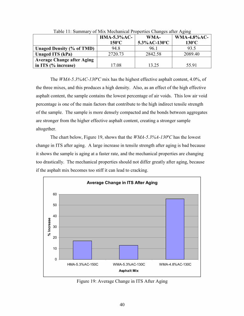
The most beneficial change in mechanical properties with the addition of

Sasobit® is the decrease in changes after aging. This indicates that there is a slower

aging process for the WMA-5.3%AC-130°C mix, which contains Sasobit®. A slower

aging process means that the life of the asphalt mix is much longer, and will last longer

when applied to pave a roadway or driveway. In turn, this saves money because

roadways will have to be re-paved, patched, and have general maintenance done less

often.

5.4 Benefits of Extending the Paving Season

The use of Sasobit® allows the HMA to be produced and compacted at a lower

than conventional temperature. This means, for those areas which have relatively short

paving seasons, for example New England, the use of Sasobit® will help in extending the

paving season. More work will get done in a typical year and hence improvements in

road conditions will be much faster.

49

5.5 Conclusion

The use of Sasobit® in WMA has the potential to reduce the asphalt industry’s

contribution to greenhouse gas emissions as well as save them money. It will reduce CO2

emissions produced both from the material and energy needed to make asphalt mixes. It

can save energy costs since an asphalt mix will not need to be heated to the conventional

temperature of 150°C, it will be able to be heated to a lower temperature, such as 130°C.

On top of all of these ecological and economic benefits, it also produces the same quality,

or better, than conventional HMA.

Not only does Sasobit® not negatively change the material properties, but it

actually produces a stronger and longer lasting asphalt mix. The addition of Sasobit®

allows better compaction of HMA, which produces lower air voids. This decrease in air

voids results in a longer lasting asphalt mix. The asphalt mixes with Sasobit® have

shown a slower aging process than conventional HMA in this study, which will result in

the longer life of a pavement.

Although Sasobit® may not be beneficial for small paving jobs, for large scale

projects it is a necessity. It can save the asphalt industry money and energy. The cost

savings come from energy costs as well as the ability to delay repaving jobs, since the

pavements containing Sasobit® have a longer in-service life.

The ecological impacts that the use of Sasobit® in asphalt mixes can have for the

asphalt industry are significant. The reduction of greenhouse gases from asphalt mix

materials and energy consumed by the asphalt industry can make a difference in the

world we live in and have the potential to improve the earth’s atmosphere. From this

study, it was calculated that 3.774 million tonnes of CO2 could be prevented from being

released into the atmosphere per year from the asphalt mix materials as well as energy

used during production. In 10 years, 37.74 million metric tons of CO2 could be

prevented. It is essential for the asphalt industry to start caring about their effects on the

environment, and the addition of Sasobit® to asphalt mixes would be a great start for

this.

50

Bibliography

1. Hurley, G.C., Prowell, B.D. Evaluation of Sasobit® for Use in Warm Mix

Asphalt. National Center for Asphalt Technology: Auburn University. June 2005. 2. Energy Information Administration. Emissions of Greenhouse Gases in the

United States 2004. U.S. Department of Energy Washington, D.C. December 2005.

3. Trumbore, D.C. Estimates of Air Emissions from Asphalt Storage Tanks and

Truck Loading. Asphalt Technology Laboratory. Owens Corning, Summit, IL.

4. Roberts, F.L., Kandhal, P.S., Brown, E.R., Lee, D., & Kennedy, T.W. Hot Mix

Asphalt Materials, Mixture Design, and Construction, Second Edition. National Asphalt Pavement Association Research and Education Foundation: Lanham, Maryland. 1996.

5. Sutton, C.L. Technical Paper T-143 Blue Smoke Emission Report. Astec:

Chattanooga, TN. 2002.

6. Environmental Protection Agency. Hot Mix Asphalt Plants Emission Assessment

Report. Research Triangle Park, North Carolina. December 2000.

7. Warm Mix Asphalt: A State-of-the-Art Review. Advisory Note 17.Australian Asphalt Pavement Association.

8. Kandhal, Prithvi S. and Sanjoy Chakraborty. Effect of Asphalt Film Thickness on

Short and Long Term Aging of Asphalt Paving Mixtures. National Center for Asphalt Technology: Auburn University. Jan 1996.

9. Hunter, Elizabeth Rae. Evaluating Moisture Susceptibility of Asphalt Mixes.

University of Wyoming. Laramie, WY. 2001.

10. Bell, Chris A. and Dan Sosnovske. Aging: Binder Validation. Strategic Highway Research Program: Corvallis, Oregon. 1994.

11. Linden, Robert N., Joe P. Mahoney, and Newton C. Jackson. Asphalt

Construction, Premature Rutting and Surface Friction Courses - Effect of

Compaction on Asphalt Concrete Performance. National Research Council: Transportation Research Record 1917. Washington, D.C. 1989.

51

Appendix A: Production of Sasobit®

Fisher-Tropsch (FT) Process

Hurley, G.C., Prowell, B.D. Evaluation of Sasobit® for Use in Warm Mix Asphalt.

National Center for Asphalt Technology: Auburn University. June, 2005. Page 6.

“In summary, in the Fischer-Tropsch synthesis, coal or natural gas (methane) is partially

oxidized to carbon monoxide (CO) which is subsequently reacted with hydrogen (H2)

under catalytic conditions producing a mixture of hydrocarbons having molecular chain

lengths of carbon (C)5 to C100 plus carbon atoms. The process beings with the generation

of synthesis gas then reacted with either an iron or cobalt catalyst to form products such

as synthetic naphtha, kerosene, gasoil and waxes. The liquid products are separated and

the FT waxes are recovered or hydrocracked into transportation fuels or chemical

feedstocks. The Sasobit® recovered is in the carbon chain length range of C45 to C100

plus. By comparison, macrocrystalline bituminous paraffin waxes have carbon chain

lengths ranging from C25 to C50. The longer the carbon chains in the FT wax lead to a

higher melting point. The smaller crystalline structure of the FT wax reduces brittleness

as low temperatures as compared to bitumen paraffin waxes.”

52

Appendix B: Testing Flow Charts

53

54

55

Appendix C: Heat Energy Calculations Heat energy required to raise the temperature of a mass, m, through delta (T), where the

mass has a specific heat of c, is given by,

Q = c*m*delta(t)

Q is in Joules

c is in Joules per gram degree C

delta (t) is in C

Consider heat required to raise temperature of aggregates

from ambient, say 25C, to 150C

Q1 c*m* 125 joules

Now consider the case where we use warm mix asphalt

Heat required to raise temperature of aggregates

from 25C to 130C

Q2 c*m* 105 joules

Savings in energy 20 joules

Savings in energy (Q1-Q2)*100/Q1

16 %

If we burn 16 % less fuel (say natural gas)

how much do we cut down CO2 production

from burning of fuel only? (percent wise?)

16 %

Add this 16 % with the cut down in CO2 production from heating HMA

It was 716.67 ppm for 150C

and 516.67 ppm for 130 C.

Hence cut down in CO2 production

27.906847 %

Total reduction in CO2 production

43.906847 percent

Savings ($) by burning less fuel

16 %

Minus cost of additive Sasobit®

added cost $ 2 per ton of mix

One ton of mix costs 60 per ton of mix

added cost 3.33 percent

56