Reform Raises Efficiency of Tea Estates in India -...

Agris on-line Papers in Economics and Informatics

Volume IX Number 2, 2017

Reform Raises Efficiency of Tea Estates in India S. Maity

Department of Economics, Assam University, Silchar, Assam, India

AbstractThis study compares the performance of the tea industry of Assam and West Bengal of India between two time stretches each spanning over six years; one ending in 2006-07 - the pre-reform regime - and the other beginning in the next year- the post-reform regime. The basic question addressed is whether reform policy led to improvement in technical efficiency of the tea industries of these states. The study uses stochastic frontier approach and introduces heterogeneity of tea gardens. Consideration of both Assam and West Bengal tea gardens adds unique flavour to this study. The study the study concludes that rehabilitation package of Indian government in the form of reform has paid off even within the existing framework of the tea gardens.

JEL Classification: C01, Q17, Q19

KeywordsStochastic Production Frontier, Technical Efficiency, Tea Gardens, Panel Data, Farm-heterogeneity.

Maity, S. (2017) “Reform Raises Efficiency of Tea Estates in India", AGRIS on-line Papers in Economics and Informatics, Vol. 9, No. 2, pp. 101 - 116. ISSN 1804-1930. DOI 10.7160/aol.2017.090209.

[101]

IntroductionTea is the most popular of all non alcoholic beverages in the world and two-third of the world population drinks 'Camellia sinensis’ (Tea). The popularity of tea has gained momentum with colonisation. Tea is commercially cultivated in the areas scattered in more than 65 countries. The major tea producing countries are India, China, Kenya, Sri Lanka, Turkey, Viet Nam, Indonesia, Bangladesh, Malawi, Uganda and Tanzania. Total tea production in the world has exceeded over 4.5 billion kgs, in 2012 where India alone contributed more than 1 billion kg of tea in 2012 and was recognised as one of the leaders in world tea production along with China (Table A1, Appendix) (Source: ITC Annual Bulletin Supplement, 2012 & MSS- March, 2013).

Tea may be placed under agriculture and also industry. It is an agricultural crop as it is grown on land and thus it is subjected to agricultural income tax. On the other hand, it is an industry in the sense that, tea is a processed commodity, and it is subjected to excise duty and cess. The tea crop involves both agricultural and industrial operations. A large amount of tea has been sold in the international markets from the very inception of this industry. As tea is placed under agriculture and industry, the concept of production efficiency is important in case

of tea industry. The consequences of the presence of inefficiency in the production process can be observed in four ways, as follows:

1. It reduces the quantity of output for a given set of inputs.

2. Some of the inputs will be either under-utilized or over-utilized.

3. There will be an increase in the cost of production.

4. There will be a loss of profit.

A production frontier gives the maximum possible output from a given set of inputs or represents minimum input bundles required to produce a given level of output given the state of technology and technical efficiency relates to the producer’s behaviour relating to the production of output with a given quantity of inputs (Kumbhakar, and Lovell, 2000). Literature abounds with the application of the measurement of efficiency by the stochastic frontier approach. The pioneering contribution in this context was made by Farrell, (1957). Later on Kalirajan, (1981), Battese, and Coelli, (1988), Ferrier, and Lovell, (1990), extended the research on efficiency estimation by using a cross section time series or panel data. Kumbhakar, et al., (1991), examined the impact of technical and allocative efficiency on the level of profits of US dairy

[102]

Reform Raises Efficiency of Tea Estates in India

farms. Battese, and Coelli, (1992), applied Frontier Production Function to an unbalanced panel data of paddy farmers in India. Battese, and Coelli, (1995), used a stochastic frontier production function for panel data on Indian paddy farms, in which the non-negative technical inefficiency effects were assumed to be a function of firm-specific variables and time.

Aigner, et al., (1977), considered stochastic frontier production functions and Schmidt and Lovell (1979) extended the earlier work by considering the duality between stochastic frontier production and cost functions - under the assumptions of exact cost minimization (considering technical inefficiency only) and of inexact cost minimization (technical as well as allocative inefficiency). Dutta, and Neogi, (2013), used the stochastic frontier approach to analyse heterogeneous panel data. Studies that have concentrated on the investigation of the tea gardens’ efficiency in India or any other tea producing country, however, are very limited. This may be because of the non-availability of reliable panel data. Studies that merit special mention in the area of measurement of technical efficiency of tea industry are by Hazarika, and Subramanian, (1999), Mahesh, et al., (2002), Basnayake, and Gunaratne, (2002) and Ariyawardana, (2003). All these studies applied stochastic frontier analysis for investigating the efficiency status of tea gardens. The first two studies were conducted for the Indian tea industry, focusing Assam tea belt, while the last two were based on the data on tea cultivation in Sri Lanka. The stochastic frontier analysis technique was utilized also to investigate the nature of technical efficiency of organic tea small holding sector in Sri Lanka (Jayasinghe, and Toyoda, 2004). Their results indicated that efficient utilization of the existing technology and labour force itself could increase production up to 55 per cents. Baten, et al. (2009 and 2010) examined the status of technical efficiency of tea-producing industry for panel data in Bangladesh using the stochastic frontier production function, by using technical inefficiency effect model. Again, Maity, (2011), Maity, (2012), examined technical and allocative efficiency by using stochastic frontier approach for the tea gardens of West Bengal and concluded that large tea gardens were relatively more efficient than medium and small tea gardens. Maity, and Neogi, (2014), examined technical efficiency status for Indian tea gardens by using panel data. But not all tea gardens efficiency related study used a parametric approach. Rather, some studies used the non-parametric approach. For example, efficiency of the Indian tea industry, considering

tea gardens of Assam and West Bengal, was investigated by using the non-parametric approach by Bhattacharjee, and Sharma, (2016).

Studies related to tea garden level efficiency measurement have generally revolved around Bangladesh, Sri Lanka and India as tea is one of the main exportable commodities from these countries. In case of India the studies have mainly focused on measuring efficiency of the tea gardens of either Assam, or West Bengal, tea belt. The present study is unique because it is based on both Assam and West Bengal tea gardens taken together. Significantly, it compares the performance of these two major tea producing states of India.

It is noted here that we have developed our model in the line of Battese, and Coelli, (1995), as well as Dutta, and Neogi, (2013). For the measurement of technical efficiency in the production of tea in Assam and West Bengal we used the stochastic production frontier approach, but we avoid using the two step procedure as it has been shown that it gives biased estimates (see Green, 2005; Fried, Lovell, and Schmidt, 2008, page 39). The methodologies used are discussed in the chapter Materials and methods.

Problem background

The present study focuses on estimating the technical efficiency for selected tea gardens of India, considering only gardens located in Assam and West Bengal. Tea is mainly grown in North India, which accounts for about 80percent of the country’s total tea production. Furthermore, even though tea is commercially cultivated in 16 states in India, Assam (52.0 per cents), West Bengal (25.8 per cents), Tamil Nadu (14.5 per cents) and Kerala (5.3 per cents) together account for more than 97.6 per cents of the total tea production. Indeed, Assam and West Bengal together contribute almost 78percent of total tea production (Table A2, in Appendix). Also, the total area under tea production in Assam and West Bengal together accounts for almost 79 per cents of the total area under tea production in India.

The Indian tea industry has a 170 years old history and it has since then contributed importantly through exports to the country’s national income. However, it has seen many ups and down in the last few years. The major problems of the Indian tea industry are: old age of tea bushes, limited availability of land in the traditional areas of tea cultivation for further extension and slower pace of replantation, the rate (0.4 per cent) is much lower than the desired (2 per cents) level, etc.

[103]


In view of these issues, for the reclamation of the tea gardens of Kerala, West Bengal and Assam, the Indian government announced certain rehabilitation packages in 2004. These packages gave the industry some breathing space and helped it to achieve better productivity. Encouraged by those positive results in 2006-07 the government further announced additional relief packages- focusing again mainly the tea gardens of Assam and West Bengal. The relief packages include, special purpose tea fund, Electronic Auction System, Setting up of a separate cell to look into the developmental needs of the small growers, Development of Geographic Information System through remote sensing, Energy conservation in small tea processing units, Organic Tea Development Project, etc.

The primary aim of this study is to compare the performance of the tea industry before and after the implementation of these relief packages. Since the relief packages focused tea gardens of Assam and West Bengal only and also it is true that Indian tea industry is largely dominated by Assam and West Bengal’s tea gardens, this study has focused on comparing the performance of the tea industry of Assam and West Bengal, probing two stretches each spanning over six years; one ending in 2006-07 - the pre-reform regime, and the other beginning in the following year- the post-reform regime. Thus the entire study period 2001-02 to 2012-13 is divided into two regimes, the pre-reform period spanning 2001-02 to 2006-07 and the post-reform period 2007-08 to 20012-13.

Other than this research objective, another objective of this study is to test the relationship between the size of the garden, measured in terms of the land area under production, and technical efficiency. Finally, in this paper author attempts to identify the major inputs or factors that influence the production of tea.

This paper is organized so as to investigate each of these research objectives in turn. The chapter Introduction reviews the literature that covers efficiency measurement leading to the justification of conducting this study. We outline the methodologies adopted, in the chapter Materials and methods. The research objectives are investigated and discused in the chapter Results and discussion. The last chapter concludes the study and suggests the induced policy measures.

Materials and methodsMaterials

This empirical study on the measurement of technical efficiency is entirely based on secondary data. The principal data source is the Tea Diary, published annually by Tea Board of India. But Tea Diary does not publish garden level panel data. Garden level panel data are collected from various garden level files maintained by Tea Board of India, Kolkata. It is to be noted here that the term “tea garden” in its present use in this paper means a collection of several individual tea farms that are producing tea under the same “garden” heading, that is, local garden names used in different areas of Assam and West Bengal. We collected data for different tea gardens from the Department of Record section of Tea Board of India, Kolkata.

The comprehensive scheme envisages the collection of reproductive data on inputs and outputs and estimation of cost of cultivation per hectare of tea for selected tea gardens of Assam and West Bengal. Garden level data were collected for the periods 2001-02 to 2012-13 and for 24 cross sections representing 24 gardens.

Methods: The model to be estimated

We have studied technical efficiency for the tea production of selected tea gardens of India using stochastic frontier approach.

Abbreviating the production function we can write our model to be estimated as:

(1)

Where y is the output, x and β stand for the vector of arguments of the production function and the vector of the coefficients respectively; all the variables being expressed in logarithm. exp(vi) is the random error term and the subscript i refers to the particular cross section.

The most commonly used forms of production functions are Trans-log and Cobb-Douglas models which are given as:

Trans-log:

(2)

[104]


Cobb-Douglas: lnyi = β0 + β1 ln ki + β2 ln li + (vi - ui) (3)

Implementation of the above model requires assumption of the form of the production function. We have implemented both the flexible trans-log form and relatively simple Cobb-Douglas form using panel data on tea production of selected tea gardens of India. A study of possible superiority of the trans-log over the Cobb-Douglas model can be tested using the log-likelihood functions. The value of the generalized likelihood-ratio (L.R.) statistic for testing the null hypothesis that the coefficients of the second order terms of the Trans-log model are jointly insignificant (i.e. βij = 0) is:

(4)

L.R. is here assumed to be asymptotically distributed as χ2 with k degrees of freedom (Coelli et al., 1998, pp.218), where k is the number of restrictions and LC-D, LT-L are maximum likelihood function for Cobb-Douglas (restricted) and Trans-log production function (unrestricted) respectively.

We once again consider equation (6). The firm specific technical efficiency (Kumbhakar, et al., 1991) which is assumed to be random variable may be written as: TEi = exp(-ui). Since , hence

, i.e., this error is one sided. So, we can write (6) as:

(5)

Here the assumptions are that and . Further ui and vi are independent of each other and also independent of xi. So, the underlying model is Normal-Truncated Normal; it was introduced by Stevenson (1980).

Our objectives are to

a) Estimate the vector β of f(xi, β) under a specific assumption on the form of production function, and

b) Estimate the technical efficiency of each producer.

In case of panel data technical efficiency may be assumed either to be time invariant or to be varying with time. If panel is a long one in time the assumption of time invariant may not be defensible unless specifically suggested by data. Battese and Coelli (1992) proposed a model for time varying technical efficiency for stochastic frontier approach with panel data. Technical efficiency effects for N cross-sections observed over T periods are defined by:

(6)

where ui are assumed to be IID truncated random variables as defined above and η, which is the focus of our attention, as it measures the efficiency trend of the tea gardens, is an unknown scale to be estimated.

Maximum-likelihood estimation (MLE) of equation (10) has been obtained by using the FRONTIER-4.1 programme (Coelli, 1996). FRONTIER programme gives the estimate of vector β, as well as well as the scalar ,

where (γ) lies between 0 and 1 depending on the dominance of σ and σu respectively. One deficiency of this programme, however, is that estimates of technical efficiency for different gardens in its present application for each period is given by it by applying the same exponential trend function on the efficiency estimate for the last period; thus only the trend values are observed and garden ranking is invariant.

Specification of variables

In this section our intention is the introduction and specification of the variables used to measure the relative efficiency of the selected tea gardens in Assam and West Bengal. The specification of model is given in the previous section. We provide now the definition of the variables used as follows:

HL = Human Labour (Wage Bill)RWW = Resources spent on Workers’ WelfareBHF = Bush Hygiene Factor PSTCD = PesticidesFERT = FertilizersIRRIG = IrrigationRRPR = Re-Plantation RequisitesCAPST = Machineries or Capital StockLND = Area under production: hectareY = Output (revenue in Rupees

per kilograms)

All the variables (including output) except land are measured in value terms, that is, in rupees lakh per hectare. The dependent variable Total Output (TOUT) is measured in terms of revenue in rupees per Kilograms to address the quality issue of tea. As tea can be of different types, the qualities and varieties can only be addressed by considering the prices paid for different types of tea and thus we consider revenue per kilogram as the output variable. The details descriptions of the variables are presented in Table 1.

[105]


Table A3 in the appendix gives the descriptive statistics of the dependent variables and various independent variables used in the estimation of SPF regression.

Results and discussionIn this section we discuss results related to the objectives of the study.

Area under production of tea in selected tea gardens of India during 2001-02 to 2012-13

The data on each input and output (both in physical and monetary terms) were collected by the full-time field man residing in the tea gardens selected for the study, on the basis of his day-to-day observations. We next consider the presentation of the average area under production for selected tea gardens through Figure 1.

It is clear from the above figure that Kakajan becomes the largest tea garden with an average area under production is 1559.41 hectares and Noweranuddy becomes the smallest tea garden with an average area under production is 236.81 hectares. There are only two tea gardens, namely Hattigor and Powai, whose average area under production are more than 900 hectares. There are altogether four tea gardens (Batabari, Noweranuddy, Nahorkutia, Lamabari and Teok) whose average areas under production are less than 400 hectares. Chubwa, Happy Valley, Dam Dim, Rungamuttee, Kellyden tea gardens have more than 700 hectares, but less than 900 hectares area under cultivation. All this information is graphically presented in Figure 1.

Classification of tea gardens in Assam and West Bengal

There exists a wide variation in the sizes of the gardens with respect to the area under cultivation, which gives us enough opportunity to divide the gardens into three categories, namely, small, medium and large. The gardens with less than 400 hectares area under cultivation are classified as small tea gardens. The gardens with more than 400 hectares but less than 600 hectares area under production is classified as medium tea gardens. Finally, the tea gardens whose area under cultivation is more than 600 hectares are tagged as large tea gardens. The classifications of the gardens are thus made purely on the basis of the areas under production in terms of hectares with the intention of checking the relationship between garden size and efficiency. Table 2 presents the classification of the gardens according to their sizes. Accordingly, we have five small, ten medium and nine large tea gardens - in Assam and West Bengal.

Cobb-Douglas versus Trans-log Model

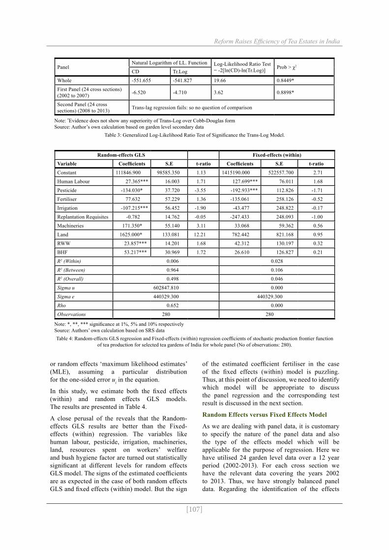
A study of possible superiority of the trans-log over the Cobb-Douglas model may be made using log-likelihood functions. The log-likelihood ration test statistic is given by the relation (4)

The test results for two panels and also for entire panel were obtained STATA-11 and are presented in Table 3.

For the first panel, the test yields insignificant result; so, we cannot prefer trans-log to be in its

Source: Author’s own specificationTable 1: Description of variables used in stochastic production frontier function of tea production for selected tea gardens of India.

Variable name Variable description

Human Labour (wage bill) (HL) Human Labour (wage bill) is measured in value term, that is, rs/hectare and is the total expenses on human labour in order to induce them to work in the tea-garden.

Resources spent on workers’ welfare Measured in value term, rs per hectare and is the sum of workers’ welfare and security and welfare sundries

Bush hygiene factor Measured in value term, rs per hectare and it includes cultivation expenses for matured tea bushes and the development costs of the area under which this cultivation are made.

Pesticides Cost in Rs per hectare. It includes costs of chemical weed control and pests & blights

Fertilizers Indicates per hectare cost of fertilizer in rupees. It includes urea, dolomite, sulphur, special foliar mixture, foliar-mop & urea spraying costs etc.

Irrigation Indicates per hectare cost of irrigation in rupees. It includes pumping, petrol costs etc.

Re-plantation requisites Indicates the factors required for immature cultivation, measured in rs per hectare. Immature cultivation means cultivation expenses required for immature tea bushes.

Machineries or capital stock Indicates per hectare expenditure on machineries. It includes machineries and equipments, machineries and equipment maintenance etc.

Area under production: hectare Indicates area in hectares under tea production.

Total output Revenue in rupees per kilograms to address the quality issue of tea.

[106]


Source: Author’s own division based on secondary dataTable 2: Classification of tea gardens in India (West Bengal and Assam) according to their size in hectares.

Size of Tea Gardens (Hectares) Number and Name of Tea Gardens

Tea gardens with land size below 400 hectares will be called in this study as the small tea gardens

Five tea gardens in West Bengal and Assam belong to this category. They are BATABARI (West Bengal), NOWERANUDDY (West Bengal), NAHORKUTIA (Assam), LAMABARI (Assam) and TEOK (Assam).

Tea gardens with land size above 400 hectares but below 600 hectares will be called in this study as the medium tea gardens

Ten tea gardens in West Bengal and Assam belong to this category. They are THURBO (West Bengal), BADAMTAM (West Bengal), BARNESBEG (West Bengal), MARGARET’S HOPE (West Bengal), SINGBULLI (West Bengal), HATHIKULI (Assam), MAJULI (Assam), NAMROOP (Assam), NONOI (Assam) and SAGMOOTEA (Assam).

Tea gardens with land size above 600 hectares will be called in this study as the large tea gardens

Nine tea gardens in West Bengal and Assam belong to this category. They are DAMDIM (West Bengal), HAPPY VALLEY (West Bengal), MAKAIBARI (West Bengal), RUNGAMUTTEE (West Bengal), HATTIGOR (Assam), KAKAJAN (Assam) , KELLYDEN (Assam), CHUBWA (Assam) and POWAI (Assam).

simpler form. However, this point here is only of academic interest, since both the forms yield positive and statistically significant giving us the same conclusion regarding the trend of efficiency. In all other cases the trans-log regression either fails or yields a smaller value for Log-likelihood Functions; so we reject the trans-log form and work with only Cobb-Douglas form in the subsequent steps.

Random-effects GLS regression and Fixed-effects (within) regression result analysis

As confirmed by the LR test the CD production function is applicable for two as well as whole panel. Thus our specified model may be presented by the following equations:

+

(7)

where, ln is the natural logarithm (i.e., to the base e).

For the purpose of estimation of the model we used FRONTIER 4.1, developed by Coelli, (1996) and STATA-11.

According to Cornwell et al (1990), for repeated observations over time, the model shall be estimated by different methods such as fixed effects ‘within’, or random effects ‘generalized least squares’ (GLS),

Source: own processingFigure 1: Area under Production (Hectare) of Tea in Selected Gardens of India during 2001-02 to 2012-13.

974.

4226

667

933.

2685

730.

0044

167

387.

7540

833

430.

733

447.

3700

833

808.

0995

458.

9669

167

531.

7086

667

413.

2584

167

442.

3916

667

716.

1419

167

1559

.409

917

746.

3506

667

462.

9634

167

544.

4842

5

411.

4134

167

256.

7312

5 737.

7588

333

674.

9647

5

482.

1088

333

296.

7193

333

280.

2355

833

236.

8132

5

0200400600800

10001200140016001800

Area

und

er P

rodu

ctio

n (H

ecta

re)

Selected Tea Gardens of India

Area under Production (Hectare) of Tea in Selected Gardens of India during 2001-02 to 2012-13

[107]


Note: *Evidence does not show any superiority of Trans-Log over Cobb-Douglas formSource: Author’s own calculation based on garden level secondary data

Table 3: Generalized Log-Likelihood Ratio Test of Significance the Trans-Log Model.

PanelNatural Logarithm of LL. Function Log-Likelihood Ratio Test

= -2[ln(CD)-ln(Tr.Log)] Prob > χ2

CD Tr.Log

Whole -551.655 -541.827 19.66 0.8449*

First Panel (24 cross sections) (2002 to 2007) -6.520 -4.710 3.62 0.8898*

Second Panel (24 cross sections) (2008 to 2013) Trans-lag regression fails: so no question of comparison

or random effects ‘maximum likelihood estimates’ (MLE), assuming a particular distribution for the one-sided error ui in the equation.

In this study, we estimate both the fixed effects (within) and random effects GLS models. The results are presented in Table 4.

A close perusal of the reveals that the Random-effects GLS results are better than the Fixed-effects (within) regression. The variables like human labour, pesticide, irrigation, machineries, land, resources spent on workers’ welfare and bush hygiene factor are turned out statistically significant at different levels for random effects GLS model. The signs of the estimated coefficients are as expected in the case of both random effects GLS and fixed effects (within) model. But the sign

of the estimated coefficient fertiliser in the case of the fixed effects (within) model is puzzling. Thus, at this point of discussion, we need to identify which model will be appropriate to discuss the panel regression and the corresponding test result is discussed in the next section.

Random Effects versus Fixed Effects Model

As we are dealing with panel data, it is customary to specify the nature of the panel data and also the type of the effects model which will be applicable for the purpose of regression. Here we have utilised 24 garden level data over a 12 year period (2002-2013). For each cross section we have the relevant data covering the years 2002 to 2013. Thus, we have strongly balanced panel data. Regarding the identification of the effects

Note: *, **, *** significance at 1%, 5% and 10% respectivelySource: Authors’ own calculation based on SRS dataTable 4: Random-effects GLS regression and Fixed-effects (within) regression coefficients of stochastic production frontier function

of tea production for selected tea gardens of India for whole panel (No of observations: 280).

Random-effects GLS Fixed-effects (within)

Variable Coefficients S.E t-ratio Coefficients S.E t-ratio

Constant 111846.900 98585.350 1.13 1415190.000 522557.700 2.71

Human Labour 27.365*** 16.003 1.71 127.699*** 76.011 1.68

Pesticide -134.030* 37.720 -3.55 -192.933*** 112.826 -1.71

Fertiliser 77.632 57.229 1.36 -135.061 258.126 -0.52

Irrigation -107.215*** 56.452 -1.90 -43.477 248.822 -0.17

Replantation Requisites -0.782 14.762 -0.05 -247.433 248.093 -1.00

Machineries 171.350* 55.140 3.11 33.068 59.362 0.56

Land 1625.000* 133.081 12.21 782.442 821.168 0.95

RWW 23.857*** 14.201 1.68 42.312 130.197 0.32

BHF 53.217*** 30.969 1.72 26.610 126.827 0.21

R2 (Within) 0.006 0.028

R2 (Between) 0.964 0.106

R2 (Overall) 0.498 0.046

Sigma u 602847.810 0.000

Sigma e 440329.300 440329.300

Rho 0.652 0.000

Observations 280 280

[108]


Note: *Evidence shows Random Effects model is appropriate Source: Author’s own calculation based on garden level secondary data.

Table 5: Hausman Test to choose between Random Effects and Fixed Effects Model.

VariablesCoefficients

Difference (b-B) S.E χ92 Prob > χ2

Fixed Effect (b) Random Effect(B)

Human Labour -127.699 27.365 -155.065 83.724

22.83 0.118*

Pesticide 192.933 -134.030 326.963 139.053

Fertiliser 135.061 77.632 57.429 251.702

Irrigation -43.477 -107.215 63.738 242.333

Replantation Requisites -247.433 -171.350 -76.083 241.888

Machineries 33.068 0.782 32.286 57.497

Land -782.442 1625.000 -2407.442 810.312

RWW 42.312 -23.857 66.170 126.375

BHF -26.610 53.217 -79.827 122.988

model we conducted the Hausman specification test. The result of this test is obtained by using STATA-11 and is presented in Table 5.

The null hypothesis related to Hausman test is that the Random Effects Model is appropriate. Table 4 shows that the value of χ2 the is 19.39 with degrees of freedom 7 and the corresponding Prob > χ2 value is 0.116. Thus, we accept null hypothesis which indicates Random Effects model will be appropriate in our case.

Analysis of efficiency levels of the teagardens

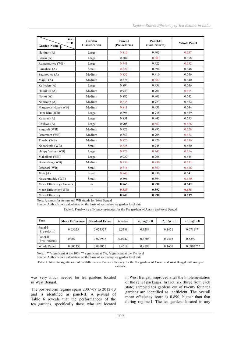
In this section discuss the results on efficiency obtained from the estimation of the model (equation 11) given in the methodology section. The results are presented in Table 6.

With the help of table-6 we will investigate our main objective- the comparison of the performance of tea estates of Assam and West Bengal in pre-reform and post-reform periods, as well as for the entire study period. This table will also help us to investigate the relationship (if any) between the size and efficiency of the tea gardens. Each pre- and post-reform period is spanning over six years; one ending in 2006-07, the pre-reform regime, and the other beginning in the following year, the post-reform regime. Twelve tea gardens from each state are considered for the purpose of comparing the performance in the post and pre-reform period. Assam consists of five large, five medium and two small tea gardens, while West Bengal comprises four large, five medium and three small tea gardens.

The mean efficiency score in the pre-reform regime is 0.847 while that in the post-reform period is 0.890. The panel mean efficiency score for the entire study period is 0.638. This mean

efficiency score is considered as the benchmark of efficiency for each panel as well as for the entire study period. This means that the garden for which efficiency score is above the panel mean efficiency, we will consider that garden is technically efficient than the other and vice-versa.

In the pre-reform period (Panel-I) the lowest efficiency score is obtained for Batabari (WB) (0.716) and the highest efficiency score is obtained for Hathikuli (A) (0.943). Considering mean efficiency of panel-I as the benchmark of comparison, we find twelve tea gardens out of twenty four as efficient. Out of these twelve efficient tea gardens seven gardens are located in Assam and remaining five are located in West Bengal. The highest efficiency score in panel-I is 0.943 for tea gardens located in Assam, obtained for Hathikuli (A) and the corresponding lowest value is 0.810 - obtained for Hattigor (A). Again, the highest and the lowest efficiency score obtained for the tea gardens located in West Bengal are 0.922 and 0.716 respectively, obtained for Singbuli (WB) as well as for Makaibari (WB) and Batabari (WB) respectively. A perusal of the complete table reveals that the performance of the Assam tea gardens in the pre-reform regime (Panel-I) are relatively better than that of the West Bengal tea gardens. In fact mean efficiency score for overall Assam tea gardens is 0.865 compared to that of the West Bengal tea gardens is 0.829. In order to test the significance of such difference we conduct t-test and the test result suggests that Assam tea gardens more efficient than that of West Bengal at 5 percent level of significance (Table 7). According to our specified benchmark for Panel-I tea gardens located in Assam turned out efficient, while that of West Bengal are inefficient. Thus we conclude that reform in the form of relief packages

[109]


Note: : ***significant at the 10%, ** significant at 5%, *significant at the 1% levelSource: Author’s own calculation on the basis of secondary tea garden level dataTable 7: t-test for significance of the differences of mean efficiency for the Tea gardens of Assam and West Bengal with unequal

variance.

Year Mean Difference Standard Error t-value

Panel-I (Pre-reform) 0.03625 0.023557 1.5388 0.9289 0.1421 0.0711**

Panel-II (Post-reform) -0.002 0.026938 -0.0742 0.4708 0.9415 0.5292

Whole Panel 0.007333 0.005051 1.4519 0.9197 0.1607 0.0803***

Note: A stands for Assam and WB stands for West BengalSource: Author’s own calculation on the basis of secondary tea garden level data

Table 6: Panel-wise efficiency estimates for the Tea gardens of Assam and West Bengal.

Year Garden Classification

Panel-I (Pre-reform)

Panel-II (Post-reform) Whole Panel

Garden Name

Hattigor (A) Large 0.810 0.903 0.637

Powai (A) Large 0.884 0.883 0.658

Rungamuttee (WB) Large 0.741 0.925 0.632

Lamabari (A) Small 0.824 0.894 0.648

Sagmootea (A) Medium 0.832 0.910 0.646

Majuli (A) Medium 0.876 0.887 0.640

Kellyden (A) Large 0.894 0.938 0.646

Hathikuli (A) Medium 0.943 0.901 0.615

Nonoi (A) Medium 0.882 0.903 0.642

Namroop (A) Medium 0.835 0.923 0.652

Margaret's Hope (WB) Medium 0.811 0.931 0.644

Dam Dim (WB) Large 0.896 0.938 0.659

Kakajan (A) Large 0.851 0.942 0.655

Chubwa (A) Large 0.908 0.662 0.626

Singbuli (WB) Medium 0.922 0.895 0.629

Batamtam (WB) Medium 0.859 0.905 0.622

Thurbo (WB) Medium 0.825 0.920 0.636

Nahorkutia (WB) Small 0.825 0.945 0.650

Happy Valley (WB) Large 0.772 0.742 0.614

Makaibari (WB) Large 0.922 0.906 0.645

Bernesberg (WB) Medium 0.759 0.836 0.631

Batabari (WB) Small 0.716 0.863 0.626

Teok (A) Small 0.840 0.930 0.641

Noweranuddy (WB) Small 0.896 0.894 0.630

Mean Efficiency (Assam) -- 0.865 0.890 0.642

Mean Efficiency (WB) -- 0.829 0.892 0.635

Mean Efficiency -- 0.847 0.890 0.639

was very much needed for tea gardens located in West Bengal.

The post-reform regime spans 2007-08 to 2012-13 and is identified as panel-II. A perusal of Table 6 reveals that the performances of the tea gardens, specifically those who are located

in West Bengal, improved after the implementation of the relief packages. In fact, six (three from each state) sampled tea gardens out of twenty four tea gardens are identified as inefficient. The overall mean efficiency score is 0.890, higher than that during regime-I. The tea gardens located in any

[110]


state performed more efficiently in the post-reform as reflected by the overall mean efficiency score. The highest and lowest efficiency score for regime-II are 0.945 and 0.742 respectively, obtained for Nahorkutia (WB) and Happy Valley (WB) tea garden respectively. It is to be noted here that both the best and worst performer belong to West Bengal. In the post-reform era tea gardens located in West Bengal are performed more efficiently than that of the Assam. In fact the overall mean efficiency score for the tea gardens located in West Bengal is 0.892, higher than that of Assam 0.890. However, the mean difference between Assam and West Bengal tea gardens turns out statistically insignificant (Table 7). Even after this from Table 5 we infer that the reform packages influence West Bengal tea gardens more positively than that of Assam tea gardens. In the post-reform period the in term of overall efficiency score West Bengal tea gardens may be categorised not only as efficient, but also that they exceed the overall mean efficiency score of Assam tea gardens. Performance wise the efficiency level of panel-II is more impressive than panel-I and it indicates that West Bengal tea gardens became more efficient than Assam tea gardens in post-reform regime. The overall performance of the tea gardens also improved after the implementation of the governmental relief packages in the post-reform regime. Thus we would conclude that the implementation of the governmental post-reform relief packages improved the status of Indian tea industry.

Another point to be noted here is that, in panel-I twelve tea gardens out of twenty four sampled tea gardens turn out inefficient. A perusal of Table 5 reveals that considering overall mean efficiency as the benchmark of efficiency, three large, five medium and four small tea gardens turn out inefficient. Thus, in panel-I 33percent large, 50percent medium and 80 per cents small sampled tea gardens turn out inefficient.

Again, in panel-II out of twenty four tea gardens, only six gardens turn out inefficient if we consider the overall mean efficiency of that panel as the benchmark. Among these inefficient tea gardens three, two and one respectively belong to category of large, medium and small tea gardens. Therefore, 33percent large and 20percent each of medium and small tea gardens are identified as inefficient. Furthermore, it is worth mentioning here that the percentage of small and medium inefficient tea gardens reduced in post-reform period compare to pre-reform period. This means that the reform packages implemented by the government influence more positively

the medium and small tea gardens than the large tea gardens. In fact the inefficiency among the small tea gardens in post-reform regime reduced to 20percent from 80percent in the pre-reform regime. The success rate is also very high in case of medium tea gardens where the inefficiency reduced from 50 per cents to 20 per cents. This again indicates that the small as well as medium tea gardens were inefficient because of structural problem which can be rectified and proper rectification can improve the level of efficiency of the concerned tea gardens.

Finally, the lowest value of efficiency is 0.614 obtained for Happy Valley (WB) and the highest value is 0.659 obtained for Dam Dim (WB) when we consider the entire study period, 2002-03 to 2012-13. Again, by considering the mean efficiency as the benchmark of efficiency, we observe that in aggregate 12 tea gardens, 8 from West Bengal and 4 from Assam turned out technically efficient. Among the technically efficient tea gardens 5, 2 and 5 gardens are classified as large, small and medium respectively. Considering the entire study period Assam tea gardens became more efficient than that of West Bengal. In fact, in terms of overall mean efficiency score, 0.635 (bench mark efficiency score is 0.638), West Bengal tea gardens turn out inefficient but Assam tea gardens remain efficient (0.640). The result of the t-test for the differences in mean efficiency of the Assam and West Bengal tea gardens are found to be significant at 10 percent level and the result is presented in table-7. Again, twelve out of twenty four tea gardens turn out inefficient if we consider entire study period. Out of twelve inefficient tea gardens four, five and three belong to large, medium and small category respectively. This means that when we consider the entire study period, 44 per cents large tea gardens while 50 per cents and 60 per cents medium and small tea gardens respectively turn out inefficient.

Thus, we may conclude that the tea gardens of Assam performed more efficiently in pre-reform period while tea gardens of West Bengal became relatively more efficient after the implementation of the reform packages in the post-reform period. However, by considering the entire study period Assam tea gardens became efficient while West Bengal tea gardens became inefficient.

After discussing the main objective of this study, we now concentrate on investigating whether our study shed light on the relationship between garden size and efficiency. For the purpose of this study, we consider in aggregate twenty-four tea gardens

[111]


and after classifying the tea gardens into three categories, namely, large, medium and small; we have information on five small, ten medium and nine large tea gardens.

As mentioned earlier that in panel-I, 33 per cents large, 50 per cents medium and 80 per cents small sampled tea gardens turn out inefficient and in panel-II 33 percent large and 20 per cents each of medium and small tea gardens are identified as inefficient. Again, by considering the entire study period in a single jargon we get 44 per cents, 50 per cents and 40 per cents large, medium and small tea gardens respectively turn out inefficient. In other words, in panel-I 77 percent, 50 per cents and 20 per cents large, medium and small tea gardens become efficient. But in panel-II situation improved for medium and small tea gardens and in both cases efficiency increased to 80 percent while in case of large tea gardens still 77 percent gardens remain efficient. When we consider entire study period in a single jargon, 66 per cents large, 50 percent medium and only 60 per cents small tea gardens become efficient. In panel-II small and medium tea gardens appear to be performing exceptionally well. But from overall performance what we would infer that large tea gardens are relatively more efficient than that of medium and small. Again, between small and medium tea gardens, with reform, medium tea gardens become relatively more efficient than the small. Thus this study concludes a direct relation between garden size and efficiency. This result supports the earlier finding by Maity, (2011) and Maity, (2012), where author found a direct

relation between garden size and efficiency by considering tea gardens of West Bengal only. The reason may be that the large gardens enjoy more specialization in terms of input utilization, managerial efficiency and at the same time large tea gardens can execute the advantage of economics of large scale production. The same result is also presented in Figure 2.

Analysis of regression result

The stochastic frontier production function in (7) can be viewed as a linearized version of the logarithm of the Cobb-Douglas production function. The inefficiency frontier model (10) accounts time-varying technical change. Maximum likelihood estimates of the parameters of the model are obtained by using a modification of the computer program, FRONTIER 4.1 (see Coelli, 1996). These estimates, together with the estimated standard errors of the Maximum-likelihood estimators, given to three significant digits, for two different panels as well as for considering entire study period are presented in Table 8.

The signs of the coefficients of the stochastic frontier are as expected, with the exception of the negative estimate of the pesticide, irrigation and replantation requisites in both pre and post reform regime as well as for the entire study period. The negative elasticities of the two variables pesticide and irrigation are quite surprising. Regarding pesticide may due to the fact that it is used more extensively as a substitute of other factors of production for getting more proper tea leave. Regarding irrigation we can say that in the tea

Source: own processingFigure 2: Trend of efficiency of selected tea gardens of India for different panel.

0

0.1

0.2

0.3

0.4

0.5

0.6

0.7

0.8

0.9

1

Tech

nica

l Effi

cien

cy

Selected Tea gardens

Panel-I Panel-II All Panel

[112]


Note: ***significant at the 10%, ** significant at 5%, *significant at the 1% level, t-values are in parenthesesSource: Author’s own calculation on the basis of secondary tea garden level data

Table 8: Maximum likelihood estimates of the stochastic production frontier function of tea production for selected tea gardens of India (No. of observations- 280).

VariablePanel-I Panel-II Whole Panel

Coeff (β) S.E. Coeff (β) S.E. Coeff (β) S.E.

Constant 5.734* (6.034) 0.950 6.625*

(9.647) 0.687 8.735* (15.227) 0.574

Human Labour 1.493* (2.966) 0.503 0.214**

(2.124) 0.101 0.587** (2.162) 0.271

Pesticide -0.574* (-2.827) 0.203 -0.007

(-0.023) 0.304 -0.18 (-0.54) 0.33

Fertiliser -0.015 (-0.059) 0.253 -0.159

(-1.010) 0.144 0.070 (0.137) 0.511

Irrigation -0.016 (-0.899) 0.018 -0.048*

(-4.170) 0.011 -0.03 (-1.06) 0.03

Replantation Requisites

-0.148* (-2.643) 0.056 -0.099*

(-2.936) 0.034 -0.020 (-0.153) 0.128

Machineries 0.686** (2.453) 0.280 0.135

(1.063) 0.127 0.717** (2.162) 0.331

RWW 1.175* (10.511) 0.112 0.648**

(2.508) 0.259 0.587* (3.895) 0.151

BHF 0.546 (1.084) 0.503 1.004*

(11.988) 0.084 0.752** (1.983) 0.379

Land 0.446 (1.331) 0.335 0.273**

(1.974) 0.138 0.868* (3.950) 0.220

Diagnostic Statistics

Variance Parameters Panel-I Panel-II Whole Panel

0.061* (5.35) 0.012 0.207***

(1.671) 0.124 2.585* (6.502) 0.398

0.050 (0.752) 0.067 0.961*

(33.504) 0.029 0.798** (2.328) 0.343

μ -0.111 (-1.057) 0.105 -0.893

(-1.612) 0.554 0.489* (2.600) 0.188

η -0.247 (-1.069) 0.231 0.243*

(2.964) 0.082 0.913* (5.633) 0.162

Log(likelihood) -10.286 -69.564 -548.381

LR test 11.799 2.021 6.102

gardens along with plenty water, proper drainage system is also needed. Again the study areas are characterized by high rainfall area. So, for these areas, drainage system rather than irrigation plays very important role for tea plantation. That is why this estimated coefficient is not only negative, but also very low in value.

Finally, the variable Replantation Requisites (RRPR) represents the factor required for immature cultivation. It is measured in value term (Rs/hectare). Immature Cultivation means cultivation expenses required for cultivation of immature tea plants. Most of the tea gardens do not maintain their own immature tea nursery; they purchase immature tea plants from the local nursery. However, they maintain mature tea

nursery alongside the garden. Perhaps because of this we get negative elasticity for this variable and the value of the estimated coefficient is low.

The estimated coefficients for the land and labour variables are 0.446 and 1.493 for panel-I, 0.273 and 0.214 for panel-II and 0.868 and 0.587 for entire study period. These coefficient estimates are highly significant, while that for costs of other inputs are relatively small though significant.

The estimate for the variance parameter, , is close to one for the second regime (panel-II), which indicates that the inefficiency effects are likely to be highly significant in the analysis of the value of output of the gardens. The value of η in Table 7 suggests that in the post-reform

[113]


regime (panel-II) efficiency showed quite an increasing and statistically significant trend. For the whole period also the trend is found to be increasing and statistically significant. However what is an important observation for the question we have posed, for the first panel (panel-I), that is, in the pre-reform regime there is absolutely no trace for efficiency improvement. So, one would suspect the observed rising trend for the whole of twelve years is the handiwork of the definite rising trend of over the later half. This result gives strong support for one to conclude that the performance with regard to technical efficiency during the post-reform regime was superior to that of the earlier period.

Conclusion The inefficiency of the tea estates can be reduced by increasing output, decreasing cost of production, increasing revenue of the tea estates, thus ultimately impacting profit. The negative values of the estimated coefficients for pesticide, irrigation and replantation requisites suggest that the tea estates have enough opportunity to improve the present condition by adopting efficient practices in these areas. Tea gardens are suggested not to use pesticide more extensively as a substitute of other factors of production for getting perfect tea leaves. Moreover, in the same line of Banerjee,

and Banerji, (2008), we would like to comment that gardens are need to use organic pesticides such as turmeric, neem, etc., so that in the international arena (market) Indian tea is not criticised for using pesticides more than the recommended doses. At the same time, by using organic and locally made pesticides, tea gardens can get more production at lower costs and they will become more cost effective as well as profitable. Again, they are recommended to improve the drainage system for the gardens rather than paying more money for irrigation as these areas are characterised by heavy rain fall (Banerjee and Banerji; 2008). By doing this they will be able to utilize their funds optimally. Replantation should be done in time with new and good quality young tea plants and for that all tea gardens are suggested to maintain nurseries for mature as well as immature cultivation. Finally, tea gardens are suggested to maintain their own nurseries for immature cultivation so that they will be able to get better baby tea plants than those purchased from outside.

The high positive values of estimated coefficients of land and labour suggest that by proper utilization of the available land and by giving appropriate training and education to the garden labourer, tea gardens can increase their level of efficiency irrespective of their size.

Corresponding author:Dr. Shrabanti MaityDepartment of Economics, Assam University, Silchar, Assam, India E-mail: [email protected]

References[1] Aigner, D., Lovell, C. A. K. and Schmidt, P. (1977) "Formulation and Estimation

of Stochastic Frontier Production Function Models", Journal of Econometrics, Vol. 6, pp. 21-37. ISSN 0304-4076. DOI 10.1016/0304-4076(77)90052-5.

[2] Ariyawardana, A. (2003) "Sources of competitive advantage and firm performance: The case of Sri-Lankan value-added tea producers", Asia Pacific Journal of Management, Vol. 20, pp. 73-90. E- ISSN 1572-9958, ISSN 0217-4561. DOI 10.1023/A:1022068513210.

[3] Banerjee, G. D. and Banerji, S. (2008B) "Tea Industry: A Road Map Ahead". Abhijeet Publication, Delhi. ISBN 8189886479.

[4] Basnayake, B. M. J. K. and Gunaratne, L. H. P. (2002) "Estimation of Technical Efficiency and It's Determinants in the Tea Small Holding Sector in the Mid Country Wet Zone of Sri Lanka”, Sri Lankan Journal of Agricultural Economics, Vol. 4, No. 1, pp. 137-150. ISSN 1391-7358. DOI 10.4038/sjae.v4i0.3488.

[5] Baten, A., Kamil, A. A. and Haque, M. A. (2009) "Modelling technical inefficiencies effects in a stochastic frontier production function for panel data", African Journal of Agricultural Research, Vol. 4, No. 12, pp. 1374-1382. ISSN 1991-637X.

[114]


[6] Baten, A., Kamil, A. A. and Haque, M. A. (2010) "Productive efficiency of tea industry: A stochastic frontier approach", African Journal of Biotechnology, Vol. 9, No. 25, pp. 3808-3816. ISSN 1684-5315.

[7] Battese, G. E. and Coelli, T. J. (1988) "Prediction of Firm-Level Technical Efficiencies with a Generalised Frontier Production Function and Panel Data", Journal of Econometrics, Vol. 38, pp. 387-399. ISSN 0304-4076.

[8] Battese, G. E. and Coelli, T. J. (1992) "Frontier Production Function, Technical Efficiency and Panel Data: With Application to Paddy Farmers in India", The Journal of Productivity Analysis, Vol. 3, pp. 153-169. E-ISSN 1573-0441, ISSN 0895-562X. DOI 10.1007/BF00158774.

[9] Battese, G. E. and Coelli, T. J. (1995) "A Model for Technical Inefficiency Effects in a Stochastic Frontier Production Function for Panel Data", Empirical Economics, Vol. 20, pp. 325-332. E-ISSN 1435-8921, ISSN 0377-7332. DOI 10.1007/BF01205442.

[10] Bhattacharjee, D. and Sharma, M. J. (2016) "Economic Analysis of Indian Tea Industry Using Non-parametric Model Data Envelopment Analysis", International Journal of Science Technology and Management, Vol. 5, No. 1, pp. 410-419. E-ISSN 2394-1537, ISSN 2394-1529.

[11] Bruno, M. (1978) "Duality, Intermediate Inputs and Value Added", In Fuss, M. and McFadden, D. (Ed.), Production Economics: A Dual Approach to Theory and Applications, Vol. 2, North Holland Publishing Co. Amsterdam. ISBN 9780444850126.

[12] Coelli, T., Rao, D. S. and Battese, G. E. (1998) "An Introduction to Efficiency and Productivity Analysis", Kluwer Academic Publishers, London. E-ISBN 978-0-387-25895-9, ISBN 978-0-387-24265-1.

[13] Coelli, T. J. (1996) "A Guide to FRONTIER Version 4.1: A Computer Programme for Stochastic Frontier production and Cost Function Estimation", CEPA Working Papers. University of North England. ISSN 1327-435X, ISBN 1863894950.

[14] Dutta, M. and Neogi, C. (2013) "Reform Raises Efficiency of Oil Refining Public Sector Enterprises in India", Indian Economic Review, Vol. XLVIII, No. 2, pp. 239-262. ISSN 0019-4670.

[15] Farrell, M. J. (1957) "The Measurement of Productive Efficiency", Journal of the Royal Statistical Society, Vol. 120, No. III, pp. 253-281. E- ISSN 1467-9868.

[16] Ferrier, G. D. and Lovell, K. (1990) "Measuring Cost Efficiency in Banking – Econometric and Linear Programming Evidence", Journal of Econometrics, Vol. 46, pp. 229–245. ISSN 0304-4076.

[17] Fried, H. O., Lovell, C. A. K. and Schmidt, S. S. (2008) "Efficiency and Productivity". [Online]. Available: http://pages.stern.nyu.edu/~wgreene/FrontierModeling/SurveyPapers/Lovell-Fried-Schmidt.pdf. [Accessed 11 Jan 2016].

[18] Government of India (2012) "Outcome Budget 2010-2011", Department of Commerce, Ministry of Commerce & Industry, pp. 1-128.

[19] Greene, W. (2005) "Reconsidering heterogeneity in panel data estimators of the stochastic frontier model", Journal of Econometrics, Vol. 126, pp. 269–303. ISSN 0304-4076.

[20] Hazarika, C. and Subramanian, S. R. (1999) "Estimation of technical efficiency in the stochastic frontier model - An application to the tea industry in Assam", Indian Journal of Agricultural Economics, Vol. 54, No. 2, pp. 201-210. ISSN 00195014.

[21] ITC Annual Bulletin Supplement (2012) and MSS March (2013) [Online]. Available: http://www.teaboard.gov.in/pdf/Global_Tea.pdf. [Accessed 12 Oct 2015].

[22] Jayasinghe, J. M. J. K. and Toyoda, T. (2004) "Technical efficiency of organic tea smallholdings sector in Sri-Lanka: a stochastic frontier analysis", International Journal of Agricultural Resources, Governance and Ecology, Vol. 3, pp. 252–265. E-ISSN 1741-5004, ISSN 1462-4605. DOI 10.1504/IJARGE.2004.006039.

[115]


[23] Kalirajan, K. P. (1981) "The Economic Efficiency of Farmers Growing High Yielding Irrigated Rice in India", American Journal of Agricultural Economics, Vol. 63, pp. 566-570. E-ISSN 1467-8276, ISSN 0002-9092.

[24] Kumbhakar, S. C. and Lovell, C. A. K. (2000) "Stochastic Frontier Analysis", Cambridge University Press, Cambridge, 1-232. ISBN 10 0521481848.

[25] Kumbhakar, S. C., Ghosh, S. and McGuckin, J. T. (1991) "A Generalized Production Frontier Approach for Estimating Determinants of Inefficiency in U.S. Dairy Farms", Journal of Business & Economic Statistics, Vol. 9, No. 3, pp. 287-296. E-ISSN 1537-2707, ISSN 0735-0015.

[26] Mahesh, N., Ajjan, N. and Raveendran, N. (2002) "Measurement of technical efficiency in Indian tea industry", Journal of Plantation Crops, Vol. 30, No. 2. ISSN 0304-5242.

[27] Maity, S. (2011) "A Study of Measurement of Efficiency". VDM Verlag Dr. Müller GmbH & Co. KG, Germany. ISBN-978-3-639-33741-9.

[28] Maity, S. (2012) "Farm size and economic efficiency: a case study of tea production in West Bengal", International Journal of Sustainable Economy, Vol. 4, No. 1, pp. 53-70. E-ISSN 1756-5812, ISSN print: 1756-5804. DOI 10.1504/IJSE.2012.043995.

[29] Maity, S. and Neogi, C. (2014) "Production of Tea in Assam and West Bengal: Technical Inefficiency Effects", Artha Vijnana, Vol. LVI, No. 4, pp. 479-499. ISSN 0971-586X.

[30] Our Bureau (2004) "IBA approves tea package", The Economic Times. February 12, 2004, Kolkata, 2.

[31] PTI (2007) "Government package helps tea gardens reopen", The Economic Times. Sep 16, 2007, New Delhi, 3.

[32] Schmidt, P., and Lovel, C. A. K. (1979) "Estimating Technical and Allocative Inefficiency Relative to Stochastic Production and Cost Functions", Journal of Economics, Vol, 9, No. Feb, pp. 343-366. ISSN 0304-4076.

[33] Stevenson, R. E. (1980) "Likelihood Functions for Generalized Stochastic Frontier Estimation", Journal of Econometrics, Vol. 13, pp. 57-66. ISSN 0304-4076.

[116]


Appendix

Source: Author’s own calculation based on ITC Annual Bulletin Supplement, 2012 & MSS, March, 2013Table A.1: Major tea producers and share in world tea production.

Country2012 2011 2010

Total Production (in m.kg) Percentage Total Production

(in m.kg) Percentage Total Production (In m.kg) Percentage

China 1761.00 38.9 1623.21 36.5 1475.06 35.2

India 1111.76 24.6 1115.72 25.1 966.40 23.1

Kenya 369.56 8.2 377.91 8.5 399.01 9.5

Sri Lanka 326.28 7.2 328.63 7.4 331.43 7.9

Vietnam 158.00 3.5 178.00 4.0 170.00 4.1

Turkey 147.00 3.2 145.00 3.3 148.00 3.5

Indonesia 130.50 2.9 142.34 3.2 151.01 3.6

Bangladesh 62.16 1.4 59.32 1.3 59.27 1.4

Malawi 42.49 0.9 47.06 1.1 51.59 1.2

Uganda 55.08 1.2 54.18 1.2 59.14 1.4

Tanzania 32.28 0.7 32.78 0.7 31.65 0.8

Others 330.87 7.3 345.16 7.8 349.45 8.3

Note: Other North Indian States includes Tripura, Uttarakhand, Bihar, Manipur, Sikkim, Arunachal Pradesh, Himachal Pradesh, Nagaland, Meghalaya, Mizoram and Oriss.Source: Author’s own calculation based on Tea Statistics (2013-14), Tea Board of India, Kolkata

Table A.2: Area under tea production and total production of tea in tea growing states in India in 2013-14.

State Area under tea ( in th. hectares) Percentage Production

(million kg) Percentage

Assam 304.40 54.0 629.05 52.0

West Bengal 140.44 24.9 312.1 25.8

Other North Indian States 12.29 2.2 23.92 2.0

Total North India 457.13 81.1 965.07 79.8

Tamil Nadu 69.62 12.3 174.71 14.5

Kerala 35.01 6.2 63.48 5.3

Karnataka 2.22 0.4 5.52 0.5

Total South India 106.85 18.9 243.71 20.2

India 563.98 100.0 1208.78 100.0

Source: Author’s own calculation based on secondary tea garden level dataTable A.3: Summary of inputs and output for selected tea gardens in India (2002 – 2013).

Variables (Rs. Lakh) Mean Maximum Minimum S.D Skewness Kurtosis C.V

Human Labour (Wage Bill) 9948.71 30349.57 32.79 5710.14 -0.06 3.35 57.40

Workers Welfare (RWW) 8179.38 16903.46 28.31 4352.57 -0.57 2.83 53.21

Bush Hygiene Factor (BHF) 4836.98 16038.87 12.83 2820.97 0.12 3.92 58.32

Pesticides (PSTCD) 3039.76 10006.14 4.98 1958.91 0.38 3.37 64.44

Fertilisers (FERT) 2808.44 7372.40 5.10 1612.59 -0.15 2.95 57.42

Irrigation (IRRIG) 572.10 2979.03 0.00 735.21 1.07 3.06 128.51

Replantation Requisites (RRPR) 879.47 3960.46 2.64 762.20 0.95 4.01 86.67

Capital Stock (CAPST) 11149.16 32017.96 31.76 6480.62 -0.03 3.14 58.13

Area under Production (LAND: hectare) 581.84 1638.68 217.18 289.67 1.59 6.08 49.79

Total Output 1009189.00 2739507.00 36.72 620012.00 0.69 3.23 61.44

Yield per Hectare 2030.44 18836.00 210.00 1086.15 12.87 200.49 53.49

Number of Observations 288 288 288 288 288 288 288

Date post:	05-Jun-2018
Category:	Documents
Upload:	vuongdieu
View:	214 times
Download:	0 times

Reform Raises Efficiency of Tea Estates in India -...

Documents