Regularization, Uncertainty Estimation and Out of Distribution Detection in Convolutional Neural Networks Ujwal Karthik Krothapalli Dissertation submitted to the Faculty of the Virginia Polytechnic Institute and State University in partial fulfillment of the requirements for the degree of Doctor of Philosophy in Computer Engineering A. Lynn Abbott, Chair Pinar Acar Creed Jones III Haibo Zeng Yunhui Zhu August 13, 2020 Blacksburg, Virginia Keywords: Regularization, Uncertainty Estimation, Classifier, Convolutional Neural Network Copyright 2020, Ujwal Karthik Krothapalli
Transcript
Regularization, Uncertainty Estimation and Out of DistributionDetection in Convolutional Neural Networks
Ujwal Karthik Krothapalli
Dissertation submitted to the Faculty of the
Virginia Polytechnic Institute and State University
in partial fulfillment of the requirements for the degree of
4.1 Confidence and accuracy metrics on the validation set of ImageNet with all
the objects removed using bounding box annotation provided by [8]. . . . . 44
4.2 Classification and calibration results with ImageNet. For a detailed explana-
tion of the metrics please refer to the ‘Experimental setup’ section. ‘A.conf’,
‘O.conf’ and ’U.conf’ refer to average confidence, overconfidence, and under-
confidence scores. We provide ECE values for 100 bins and 15 bins mean
scores along with their standard deviation (std). . . . . . . . . . . . . . . . 52
xxiv
4.3 Classification and calibration results with OpenImages. For a detailed expla-
nation of the metrics please refer to the ‘Experimental setup’ section. ‘A.conf’,
‘O.conf’ and ’U.conf’ refer to average confidence, overconfidence, and under-
confidence scores. We provide ECE values for 100 bins and 15 bins mean
scores along with their standard deviation (std). . . . . . . . . . . . . . . . 54
4.4 Fine-tuning on MS-COCO using FRCNN for object detection. For a detailed
explanation of the results please refer to the ‘Experimental setup’ section.
AP refers to average precision and AR refers to average recall at the specified
Intersection over union (IoU) level. We also provide AP values for small,
medium, and large objects using ‘S’, ‘M’, and ‘L’ respectively. . . . . . . . . 55
xxv
Chapter 1
Introduction
Categories are ubiquitous in almost all datasets. Classification can be defined as the problem
of recognizing the category of a given observation. Classification is a well studied statistical
problem with a significant amount of progress made in the past decade. It is the basic
building block of many applications pertaining to the areas of Computer Vision, Speech
Recognition and Natural Language Processing. To train a good classifier, usually a large
number of diverse (independent and identically distributed) samples are needed and it is
important to prevent the classifier from overfitting to the training samples.
The task of classifying/identifying objects in images is very easy for humans with good vision
capabilities however, machines have a difficult problem of relying on millions of pixel values
to produce a probability distribution for the same classification task. The human visual cor-
tex is very advanced compared to the state of the art artificial neural networks. The latest
advances in the field of deep neural networks (DNNs) show that surpassing human capabil-
ity when it comes to certain computer vision tasks is possible. Deep convolutional neural
networks (CNNs) have been used for solving various computer vision problems, especially
image classification [40] with tremendous success using large datasets since 2013 [32, 60]. By
pairing the hierarchical approach of DNNs with cross-correlation operations, CNNs can learn
complex representations required for classification. Overfitting in this context refers to the
phenomenon of simple memorization of the input samples by the CNN (model) rather than
reasoning about the salient features of the samples so the classifier may not generalize to
1
2 Chapter 1. Introduction
unseen samples. With ever increasing size of neural networks [25, 61], there is a need for
vast amount of labeled data [47] and better generalization, as simply increasing the number
of parameters in a neural network will often lead to overfitting of the training data. Model
capacity is defined as the ability of a model to learn complex tasks, and a larger model
usually will be able to approximate and learn to represent more complex data distributions.
Training data and an objective function are some of the first design choices that one must
consider when training a classifier. Modern day CNNs have a large number of parameters
and often suffer from many problems when deployed in the real world. Lack of diverse train-
ing data is one of the problems. A popular class of methods used to improve the diversity
of training data is known as data augmentation.
f( )
x
Dogf(x)
Classifier
Figure 1.1: The general idea of a classifier, x is the input to a learned function f whichoutputs a class label. Future discussions of classifiers in this dissertation will refer to a CNN(f ) that takes an input color image (x) and outputs a class label.
As shown in figure 1.1, a classifier can be understood as a function f that maps a given input
to a class label. To learn f, the classifier is supplied with a finite number of examples from
3
the training dataset. The learnt parameters of a classifier are often referred to as weights. In
the case of CNNs, an input layer is the part of a CNN that takes the raw input and outputs
a representation of the input. In the case of images, the input layer usually consists of simple
image operations like edge detectors that have been learnt.
The output layer of a classification CNN is usually a vector whose length is equal to the
number of classes present in the training data. Any layer that is sandwiched between an
input layer and an output layer of a neural network is referred to as a hidden layer, as shown
in figure 1.2. To solve complex problems, a higher number of hidden layers are used as
this allows the neural network to approximate complex distributions of data. The ability
of a neural network to learn nuanced differences in the data is referred to as the network’s
expressive power. The higher the number of hidden layers the higher the expressive power
of the classifier. In the case of a simple square RGB image with each side equal to 224 pixels
and each pixel having an intensity of 0 to 255, the number of possible images is extremely
large, 2563×224×224 to be precise. The classification CNNs in this dissertation are trained to
detect 1000 different classes of images, as the popular ImageNet 1-K [60] dataset consists
of 1000 classes and is often used by researchers to benchmark new approaches for classifying
data. So in this case, the CNN is taking raw input from a very large space and learning to
represent the input in a much smaller space, 1000 in our case. We also have trained CNNs
on the popular OpenImages dataset, and we identify these experiments separately.
4 Chapter 1. Introduction
1 32
6 28
16 10
1 120
1 84
10
SOFT
Figure 1.2: LeNet-5 [40], a CNN used for high accuracy digit recognition. Yellow coloredlayers are convolutional layers, red colored layers are max-pooling layers and teal coloredlayers are fully connected layers. The layers that are not directly connected to input andoutput (last layer in this figure) are called hidden layers. The output layer is shown inmagenta. Figure plotted using the implementation of [31].
1.1 Background
1.1.1 Regularization
Training large CNNs has been possible with the tremendous compute power available nowa-
days. However, a large model requires a large training dataset and collecting large datasets
is expensive computationally, manually and logistically. In order to generalize well, a clas-
sifier should perform as accurately on unseen examples as it did on seen examples during
training. Regularization of a classifier refers to the idea of improving the classifier’s gen-
1.1. Background 5
eralization performance when a finite number of training samples are present. Since 2013,
numerous data augmentation and regularization methods have been proposed and are a part
of standard training procedure for CNNs [28, 32, 63, 67]. In order to prevent simple memo-
rization of the training data (over-fitting) and to constrain the complexity of the classifier,
strong regularization is needed. Figure 1.3 shows a flowchart of the steps typically followed
in the process of training a classifier. Data augmentation has proven to improve classifier
performance at no additional computational cost at test time and is a very active area of
research. Categorical labels are used for training CNNs. These labels indicate which class
(category) of object is present in a given image. These labels do not have any information
on the location of the object in a given image.
The goal of this work is to show that regularization of existing classifiers can also be done
using labels that are not only categorical but also with labels that localize the relevant object in
a given image. We explore the idea of using the labels that localize the object to train better
classifiers and object detectors as this is a very active area of research [32, 60, 69, 74].
Early stopping of the training scheme to prevent over-fitting, dropout (dropping hidden
layer activations randomly while training) and weight decay (penalizing the norm of the
model’s parameters) fall under the umbrella of explicit regularization methods, whereas
image operations such as randomly cropping a subregion, randomly changing the aspect
ratio and randomly adding a positive or negative value to the pixel intensities of an image
fall under the umbrella of data augmentation methods. Some of the data augmentation
methods can be applied in the feature (hidden) space and these methods are then closer to
explicit regularization methods (for example, [63]).
Dropout [63], when applied to the input layer of a CNN, is a type of data augmentation
commonly known as random noise data augmentation. The neural activations of the hidden
layers of the CNNs are easily confused by texture as opposed to the shape of the object [19].
6 Chapter 1. Introduction
However, when some of the new data augmentation methods are used, the classifier (model)
learns shape specific features of the objects rather than focusing on just their texture. This
is one of the several motivating factors for our work.
Randomly dropping hidden layer activations as proposed in dropout [63] and randomly
dropping part of input pixels as [13, 20, 62, 79] have improved the ability of CNNs to
localize and classify objects in a given image. All the above mentioned data augmentation
methods have a regularization effect and most of the methods can be used in conjunction
with one another after empirical validation, as the theory behind such methods is not fully
understood.
Our regularization method is called CopyPaste and is inspired by the state of the art ap-
proaches described above.
1.1. Background 7
1.1.2 Adaptive Label Smoothing
Examples of random crops and labels generated by adaptive label smoothing during training
H
Sample Our label = 1- α = 𝑤ℎ
𝑊𝐻
0.40
0.60
0.14
0.40
W
w
h
w
h
w
h
w
h
0.270.290.14
0.160.430.25
0.0170.0180.016
Figure 1.4: Random crops of images are often used when training classification CNNs to helpmitigate size, position and scale bias (left half of figure). Unfortunately, some of these cropsmiss the object as they do not have any object location information. Traditional hard labeland smooth label approaches do not account for the proportion of the object being classifiedand use a fixed label of ‘1’ or ‘0.9’ in the case of label smoothing. Our approach (righthalf) smooths the hard labels by taking into account the objectness measure to compute anadaptive smoothing factor. The objectness is computed using bounding box information asshown above. Our approach helps generate accurate labels during training and penalizes low-entropy (high-confidence) predictions for context-only images (the main object is completelyor mostly absent).
We introduce the concept of adaptive label smoothing in this dissertation. Modern CNNs
are overconfident in their predictions [27, 37]. Overconfidence in this context refers to the
problem where a classifier predicts the wrong label with a high confidence. CNNs also suffer
from reliability issues as they are miscalibrated to begin with [23], and miscalibration refers
8 Chapter 1. Introduction
to the gap in accuracy and confidence of a classifier. There is a growing demand for labeled
data [47] to improve generalization performance, as increasing the number of parameters
in a neural network [64, 76] will often lead to overfitting of training data, and obtaining
an exponentially large labeled dataset is very expensive. Safely deploying deep learning
based models has become an immediate challenge [2] as CNNs are being used in a variety
of applications. As a community, apart from obtaining high accuracies, we also need to
provide reliable uncertainty measures of CNNs. By having reliable confidence measures,
we can improve precision (the number of correct predictions divided by all the predictions
pertaining to a class) by not acting with certainty when uncertain predictions are produced,
as in the case of safety-critical systems.
Regularization is key in improving generalization and minimizing overfitting characteristics
of CNNs. Any change to the learning algorithm of a classifier that improves the general-
ization performance but does not reduce the classifier’s training error can be referred to as
regularization in this context. In the case of classification CNNs, ground-truth labels are
typically provided as a one-hot representation of class probabilities. These labels consist of
0s and 1s and if the number of classes are K, the label vector has a single 1 indicating the
pertinent class in a given label vector of length K with K − 1 0s. Recently [66] employed
label smoothing, providing soft labels that are a weighted average of the hard targets and the
uniform distribution over labels during training to improve learning speed and generalization
performance. Usually, in the case of label smoothing, the index corresponding to the rele-
vant label of a given training image has a value of 0.9 and all the other indices in the vector
have a value of 0.1/(K − 1). Soft targets improve the training signal by not providing hard
targets to compute the cross entropy loss but a weighted average with a uniform distribution
over all classes using a fixed smoothing factor [50, 66]. Label smoothing minimizes the gap
between the logits (unnormalized log probabilities output by CNNs) of the classes and shows
1.1. Background 9
improvement in learning speed and generalization; in contrast, hard targets tend to increase
the values of the logits and produce overconfident predictions [50, 66]. We illustrate the
different labels used by CNNs in figure 1.4.
Object detection [21] is a well-studied problem and most approaches need bounding box
information during training. Recently, [16] proposed using novel synthetic images to im-
prove the object detection performance by augmenting training data using object location
information. However, classification CNNs have not exploited bounding box information
to regularize CNNs on large datasets to our knowledge. The concept of ‘Objectness‘ was
first introduced by [1], and the role of objectness has been studied extensively since then.
Quantifying the likelihood an image window contains an object belonging to any class makes
the measure class agnostic.
When training a classifier, cross entropy loss is employed but it does not penalize incorrect
spatial attention, making CNNs often overfit to context or texture rather than the pertinent
object [19], as shown in the left half of figure 1.4. The bottom row displays samples
with negligible amounts of ‘Dog’ pixels and traditional methods would label them as ‘Dog’,
causing CNNs to output incorrect predictions with a high confidence when presented with
images of backgrounds or just context. Adaptive label smoothing (our approach) involves
using bounding box information to smooth the hard labels of a classifier, as displayed to the
right in figure 1.4. Traditional approaches [32, 60, 69, 74] use random resize and random
crop augmentation, and sometimes lose the pertinent object in the training sample. Our
approach adapts label smoothing by deriving the smoothing factor using the objectness
measure. When compared to approaches based on hard labels, sample mixing and label
smoothing, our approach improves object detection and calibration performance.
10 Chapter 1. Introduction
1.2 Challenges
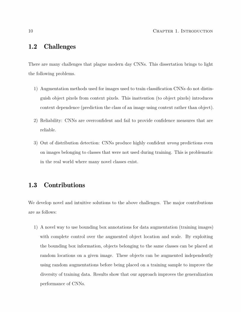
There are many challenges that plague modern day CNNs. This dissertation brings to light
the following problems.
1) Augmentation methods used for images used to train classification CNNs do not distin-
guish object pixels from context pixels. This inattention (to object pixels) introduces
context dependence (prediction the class of an image using context rather than object).
2) Reliability: CNNs are overconfident and fail to provide confidence measures that are
reliable.
3) Out of distribution detection: CNNs produce highly confident wrong predictions even
on images belonging to classes that were not used during training. This is problematic
in the real world where many novel classes exist.
1.3 Contributions
We develop novel and intuitive solutions to the above challenges. The major contributions
are as follows:
1) A novel way to use bounding box annotations for data augmentation (training images)
with complete control over the augmented object location and scale. By exploiting
the bounding box information, objects belonging to the same classes can be placed at
random locations on a given image. These objects can be augmented independently
using random augmentations before being placed on a training sample to improve the
diversity of training data. Results show that our approach improves the generalization
performance of CNNs.
1.4. Outline 11
2) A classifier whose confidence is grounded in object size. We develop a novel way to force
a CNN to produce confidence values that correspond to the relative object proportion
in a given image. We show that this approach improves localization performance and
produces more reliable predictions.
3) Out of object detection by generating high entropy/low confidence predictions on un-
seen data. Using this approach we can neglect predictions whose confidence is below
a certain threshold, thereby improving precision.
1.4 Outline
This dissertation is organized as follows.
1) Chapter 1: Provides an introduction to this dissertation.
2) Chapter 2: Provides an overview and history of CNNs.
5) Chapter 5: Presents our work on Out of Distribution Detection.
6) Chapter 6: We summarize our work and describe exciting new directions for future
work.
12 Chapter 1. Introduction
Begin
Collect data and append class labels to each sample
Regularize
Train a classification model
If (NOT overfitting AND NOT underfitting)
false
true
Split data into train, validation and test datasets
End
Increase/decrease model complexity
Figure 1.3: A typical flow process of training a classifier is shown. The fourth step representsthe theme of the work being pursued.
Chapter 2
Overview
This chapter of dissertation will introduce the history and theory behind deep learning in a
supervised setting and provide motivation for this work. A detailed description of related
work is also provided.
2.1 Deep Learning
The subsections will describe the history behind modern Convolutional Neural Networks
(CNNs) beginning with the idea of a Neuron and then Multi-Layer Perceptrons (MLPs).
2.1.1 Neurons, Perceptrons and Multi-Layer Perceptrons
The idea of an artificial neuron can be traced to 1943 when Warren McCulloch and Walter
Pitts proposed the McCulloch-–Pitts neuron. The authors presented a mathematical basis
to model an artificial neuron with inputs and a binary output. The McCulloch-–Pitts neuron
was modeled to accept multiple binary inputs xi which were multiplied by the weights wi
(represented between -1 and +1). The values wixi were then summed to compute a weighted
sum S. The neuron is said to have fired when the weighted sum S was greater than a
threshold T [48]. The threshold T is also called an activation function. The neuron was
able to perform logical operations like AND, OR and NOT by using appropriate thresholds
13
14 Chapter 2. Overview
and inputs. The activation function of the McCulloch-–Pitts neuron is a step function or a
Heaviside function. Mathematically, the weighted sum S is computed using the equation:
S =n∑
i=1wixi (2.1)
The output y of the McCulloch-–Pitts neuron is a binary variable. The output can be 0 or
1 and is computed using the equation:
y = f(s) =
1 for s ≥ T
0 for s < T(2.2)
Figure 2.1: A simple neuron.
The neuron was improved to a linear classifier called the Perceptron by Frank Rosenblatt in
1958 [59]. The perceptron was essentially a binary classifier. The perceptron added another
parameter to the McCulloch-Pitts neuron called bias. The bias is a constant weight in the
case of the perceptron and can take a value of -1 or +1. The output of the perceptron
could be +1 or -1. The weights of a perceptron can be ‘learnt’ using a technique developed
by Donald Hebb called Hebbian Learning [26]. Adding the bias term to 2.1 changes the
2.1. Deep Learning 15
mathematical representation to:
S =n∑
i=1wixi + b (2.3)
The weight updates can be represented as:
∆wij = ηyjxi (2.4)
Learning the perceptron is made possible by using the wij which is referred to the weight
update. The weight update is equal to the product of learning rate of the perceptron η, the
inputs xi and the output yj.
Figure 2.2: A simple perceptron.
Limitation of the perceptron was the input data had to be linearly separable. Apart from
simple logic gates, non-linearly separable cases like XOR could not be solved using the
perceptron model.
In 1989, George Cybenko published the idea of using a combination of linear perceptrons to
approximate continuous functions [11]. These networks are also called Feed Forward Neural
Networks (FFNNs) as the inputs are fed in the forward direction to layers of perceptrons.
16 Chapter 2. Overview
The architecture of FFNNs is simple, a layer of perceptrons feeds the next layer and this
process connects the input layer with that of the output with multiple hidden layers. To
train FFNNs, backpropagation is employed, this method takes advantage of the chain-rule to
propagate the updates. The weights of the network are updated based on the error measured
at the output layer and propagated all the way back to the input layer in a layer by layer
fashion. When backpropagation is performed in an iterative fashion over all the samples in
a training set, the process is called gradient descent.
2.1.2 Convolutional Neural Networks
The Multi-Layer Perceptrons (MLPs) were extended to work with images. In 1980 Kunihiko
Fukushima proposed the Neocognitron. By using a combination of simple and complex cells
the Neocognitron was able to provide translational invariance for recognition tasks [18].
The term Convolutional Neural Network (CNN) was popularized by LeCun et al. in 1990. It
was used to classify handwritten digits with an accuracy of 99% [41]. The model was called
‘LeNet’, the network was able to classify handwritten digits with variance in position, scale
and appearance.
CNNs evolved with the advent of parallel computing resources like GPUs and the availability
of labeled data. In 2012 a CNN called “AlexNet” by Krizhevsky et al. formally brought the
methods to a wide audience by competing in the 2012 “ImageNet” challenge and surpassing
all classic computer vision baselines. The AlexNet enabled modern CNNs which are being
used every day by consumers all over the world.
Convolutional neural networks have a computational advantage over FFNNs that are fully
connected, the number of parameters are minimized in a CNN because of weight sharing
of neurons. Spatial and shift invariances are a result of the shared parameters and pooling
2.1. Deep Learning 17
1 32
6 28
16 10
1 120
1 84
10
SOFT
Figure 2.3: LeNet-5, a CNN used for high accuracy digit recognition [39].
layers.
Convolution in this case is an operation involving two functions like, f which is the input
and g the kernel. The result of convolution can be represented by h. The function h can
be computed by integrating the overlap of f and g. In a signal processing approach this is
represented as:
h(t) = (f ∗ g)(t) =∫ ∞
−∞f(δt)g(t − δt) dδt (2.5)
The convolution operation is commutative and when the inputs are images, we can discretize
the above equation and can work in the integer space. Also the convolution needs to be per-
18 Chapter 2. Overview
formed over two dimensions in the case of images. The convolution operation with kernel K
over image I is progressed by the sliding window method. The kernel K is slid incrementally
over the input image producing a feature map H. Mathematically:
H(i, j) = (I ∗ K)(i, j) =∑m
∑n
I(m, n)K(i − m, j − n). (2.6)
To suppress the unimportant regions in the feature maps, a pooling operation layer is em-
ployed in the network, this layer also reduces the image dimensions. The common types of
pooling layers are Max pool and Average pool. This layer adds some spatial invariance to
the network as well. Simply composing a network with multiple convolutional and pooling
layers is not enough, to inject non-linearity, a transfer function is employed. A rectified
linear unit or (ReLU) is one of the most commonly used activation or transfer functions.
The output of ReLU differs from that the sigmoid function as ReLU is not limited between
0 and 1. The lower bound of ReLU and sigmoid functions is 0 and their outputs are always
positive. The ReLU’s upper bound is the input itself x.
The final layer of the network is known as the output layer and the output is a vector with
a number of elements equal to the classes in the training data in the classification setting.
To obtain the class probabilities a specific layer known as a softmax layer is used after the
final layer. To train a CNN, a gradient descent approach is used typically. In the context of
this dissertation, all the methods use a modified Stochastic Gradient Descent (SGD) with
Nesterov momentum to minimize the cross entropy loss. For a more thorough understanding
of the various layers and optimization methods used in the training of CNNs please refer to
[22] as a detailed discussion of these methods is out of scope of this document.
Chapter 3
CopyPaste
This chapter is dedicated to our regularization technique called, CopyPaste.
3.1 Datasets
We evaluate our classification approach on the ImageNet-1K dataset [60]. The dataset con-
sists of about 1.28M million training images and 50 thousand validation images with 1000
categories (classes). In addition to class labels, about 38 percent of the training images have
2 dimensional coordinates specifying a rectangular bounding box to enclose the pertaining
object. We use the bounding box annotations for these images in our approach for classifi-
cation. ImageNet pre-trained models are used for many other visual recognition tasks like
object recognition. And to evaluate the object detection performance, we use the MS-COCO
dataset [44]. It has 80 object classes for object detection and there are about 118 thousand
images for training and 5 thousand images for validation. We also evaluate on Pascal VOC
2007 and 2012 [17] trainval data of about 33 thousand images and 20 categories. The
object detection models are then validated on VOC 2007 test data consisting of about 5
thousand images.
19
20 Chapter 3. CopyPaste
x
x1
x2
f( )
Dogf(x)
Classifier
Figure 3.1: In a classification approach, the location of the object is not accounted for whiletraining and the expected outputs (post training) for all the 3 variations of the image shouldindicate Dog. The CNN has to learn to localize the pertinent object (dog in this case) andproduce an output indicating the presence of the object.
3.2 Approach
In the past year, CNNs that have been trained using numerous data augmentation approaches
have shown state of the art performance on standard datasets [69, 74] and our approach
is inspired by them. The standard training of CNNs on images, including the recent data
augmentation approaches are based on the idea that for a classification problem as long as
the object corresponding to the class is present in any location in a given image then the
label of the image is the same as that of the object as shown in figure 3.1. In a given image,
the location of the object is irrelevant to a classification CNN and the CNN has to learn to
localize and suppress the context and other irrelevant objects in the image. This is true for
3.2. Approach 21
+ =
Figure 3.2: Our method uses bounding box information to paste objects belonging to thesame class in a given image. The red bounding box is an example of bounding box annotationand the rest of the image is considered context. The green bounding box shows the objectthat has been pasted from another image of the same class if bounding boxes are available.The bottom two rows are sample images generated on the fly by our approach. The labelsof images in the second row (left to right) are, ‘Goldfish’, ‘Cauldron’, and ‘Alligator lizard’.The labels of images in the third row (left to right) are, ‘Tench’, ‘Snow leopard’, and ‘Robin’.
all strict classification problems.
Our approach involves using bounding box information to augment the training dataset for
a classification task. The location of the object in a given image is specified by a rectangular
bounding box. In the first row of figure 4.1, red dotted lines are used to illustrate a bounding
box. Using bounding box annotations to address object detection is well studied [21], but
it has not been used in classification problems for augmentation to our knowledge on the
ImageNet dataset. Nikita et al. [16] have shown that using the training data to create novel
synthetic images and respecting the context can improve the object detection performance.
22 Chapter 3. CopyPaste
However, even the most recent approaches in the area of classification do not incorporate
bounding box information of the objects present in them. We use bounding box information
when available during training of our classifier by identifying the class of a given image and
pasting an object of the same class on it. Figure 4.1 shows our approach on some of the
training samples. The bottom two rows are samples generated by our approach. We use
objects and paste them anywhere in a given image, the intuition being that objects of the
same class share similar context. Our approach is label preserving because we do not have to
change the labels of our transformed images. We can generate infinitely many combinations
of objects and context at different scales and locations. This is a powerful way to regularize
CNNs. Our approach also improves classification performance, small object detection and
localization in general.
Figure 3.3 shows the differences between our method and the other recent approaches. Cut-
Mix and RICAP change the label of an image based on the proportion of pixels represented
by each class and the ‘mixing’ of samples is random. Our method is label preserving (correct
labels are passed to the classifier during training) as opposed to CutMix and RICAP which
use random crops to mix samples from different classes. Incorrect labels hurt the training of
CNNs, and CutMix and RICAP often use context crops instead of object crops, but supply
the label of the object in the image to the CNN. We argue that this inconsistency can lead
to context dependence as the authors of RICAP [69] point out in their work.
3.3 Contributions
In this chapter, we have contributed to the research of data augmentation approaches for
classification CNNs. The contributions include:
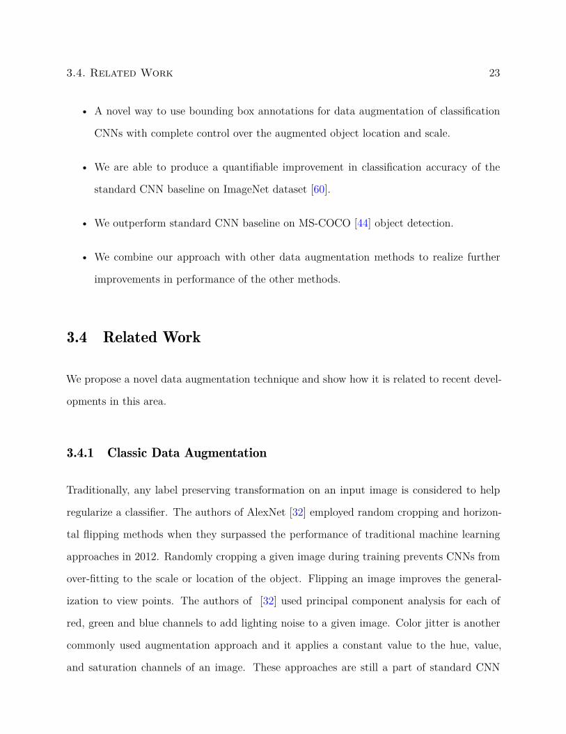
3.4. Related Work 23
• A novel way to use bounding box annotations for data augmentation of classification
CNNs with complete control over the augmented object location and scale.
• We are able to produce a quantifiable improvement in classification accuracy of the
standard CNN baseline on ImageNet dataset [60].
• We outperform standard CNN baseline on MS-COCO [44] object detection.
• We combine our approach with other data augmentation methods to realize further
improvements in performance of the other methods.
3.4 Related Work
We propose a novel data augmentation technique and show how it is related to recent devel-
opments in this area.
3.4.1 Classic Data Augmentation
Traditionally, any label preserving transformation on an input image is considered to help
regularize a classifier. The authors of AlexNet [32] employed random cropping and horizon-
tal flipping methods when they surpassed the performance of traditional machine learning
approaches in 2012. Randomly cropping a given image during training prevents CNNs from
over-fitting to the scale or location of the object. Flipping an image improves the general-
ization to view points. The authors of [32] used principal component analysis for each of
red, green and blue channels to add lighting noise to a given image. Color jitter is another
commonly used augmentation approach and it applies a constant value to the hue, value,
and saturation channels of an image. These approaches are still a part of standard CNN
24 Chapter 3. CopyPaste
training. However, they are not sufficient to reduce the effect of over-fitting on their own,
as newer CNN architectures can have almost 100 million parameters and billions of floating
point operations.
3.4.2 Random Noise
The random noise class of data augmentation methods [13, 79] work by masking random
regions of an input image with zeros. These methods may accidentally erase the pertaining
object in a given image, forcing the CNN to rely purely on context at times to make a
prediction. Relying on context only is not an efficient way to train neural networks. This
approach can also be applied to the inputs of hidden layers (also known as feature space)
as well. The authors of DropBlock [20] have used this technique (applying random noise to
the feature space) to obtain better generalization. The authors of [7, 62]use random noise
based methods to obtain better localization characteristics.
3.4.3 Mixed Sample
In the case of classification CNNs, the ground truth/labels are represented by a one-hot
representation of class probabilities. These labels consist of 0s and 1s, with a single 1
indicating the pertinent class in a given label vector. The latest work in the area of data
augmentation involves using samples from different classes and changing the expected output
of the CNN to output a probability distribution based on the number of pixels/intensity of
pixels represented by each class.
The authors of Mixup [70, 77] use alpha blending (weighted sum of pixels from two different
classes) and apply the blending weights to the corresponding labels. The authors of [74]
show that Mixup is detrimental to the performance as the generated images are not natural
3.5. Object and Context based Data Augmentation 25
as opposed to cut-paste methods like RICAP and CutMix.
Having soft labels (label values in between 0 and 1) is an advantage while training CNNs as
the probabilities output by a CNN are never perfect 0s and 1s and the CNNs usually produce
overconfident results even when their predictions are wrong. The authors of CutMix and
RICAP [69, 74] also use soft labels in their approach. In our case since the samples being
mixed are from the same class, we do not have to change the label. This allows for easy
integration with CutMix and RICAP [69, 74] as well.
3.4.4 AutoAugment
In order to learn the best augmentation strategy dynamically during training, the authors of
AutoAugment [10] use reinforcement learning to learn the best combination of existing data
augmentation methods.
3.5 Object and Context based Data Augmentation
In this section, we describe the data augmentation methods of interest in mathematical
detail.
Consider D = ⟨(xi, zi)⟩Ni=1 to be a dataset consisting of N independent and identically
distributed real-world images belonging to K different classes. Let X represent the set of
images, and let Y denote the set of ground-truth class labels. Sample i consists of the image
xi ∈ X along with its corresponding label zi ∈ Y = {1, 2, ..., K}. Let fθ represent the
CNN classifier with model parameters θ. The predicted class is yi = argmaxy∈Y pi,y, where
pi,y = fθ(y|xi) is the computed probability that the image xi belongs to class y.
Let zi represent the one-hot encoding of label yi.
26 Chapter 3. CopyPaste
In the case of Mixup with two samples, (xi, zi) ∼ D and (xj, zj) ∼ D, the transformed image
and label pair (x, z) are computed as,
x = λxi + (1 − λ)xj (3.1)
z = λzi + (1 − λ)zj (3.2)
where λ ∼ Beta(γ, γ) and γ is a hyperparameter set to 0.3 by default.
In the case of RICAP with 4 samples, (x1, z1) ∼ D, (x2, z2) ∼ D, (x3, z3) ∼ D and (x4, z4) ∼
D. The authors patch the upper left, upper right, lower left, and lower right regions of the
four images to generate a new sample.
Let W and H denote the proportions of the original image.
To crop the four images k following the sizes (wk, hk), the authors generate the coordinates
of the upper left corners of the cropped areas randomly.
The ratio Wi is computed proportional to the area occupied by each patch from one of the
four images. The label z is computed as:
z =∑
k∈{1,2,3,4}Wkzk (3.3)
where Wk = wkhk
WH(3.4)
In the case of CutMix with two samples, the label z is computed as:
z =∑
k∈{1,2}Wkzk (3.5)
3.6. Experiments 27
where Wk = wkhk
WH(3.6)
Our method is called CopyPaste and it is used to generate a new training sample (x, z) by
combining two training samples (xi, zi) and (xj, zj) from the same class.
The training sample (x, z) is used to train the model with the same label as the classes of
both samples are the same. We use the 480K images from the ImageNet dataset that have
bounding box annotations and the label remains unchanged.
z = zi (3.7)
For implementation, we use a network storage as our approach continuously changes the
proportion of original samples and CopyPaste-d samples over the course of training and is
compute intense. We handle our augmentation operation using a dedicated node.
Our approach can be used without any changes to the loss function or the network architec-
ture.
We use traditional data augmentation methods and scale/crop objects before pasting them
on images of the same class. We believe this helps our performance when detecting small
and multiple objects.
3.6 Experiments
We show results using extensive experiments on both classification and object detection
tasks.
28 Chapter 3. CopyPaste
Table 3.1: ImageNet classification accuracies using ResNet-50 architecture. ‘*’ denotes re-sults reported in their paper.
Model # Parameters Top-1Err (%)
Top-5Err (%)
ResNet-50 (Baseline) 25.6 M 23.28 6.92ResNet-50 + RICAP [69] 25.6 M 21.9 6.17ResNet-50 + CutMix [74] 25.6 M 21.60 6.04ResNet-50 + DropBlock* [20] 25.6 M 21.87 5.98ResNet-50 + CutMix [74] + CopyPaste 25.6 M 21.48 5.85ResNet-50 + RICAP [69] + CopyPaste 25.6 M 21.75 6.16ResNet-50 + CopyPaste 25.6 M 22.23 6.376
3.6.1 ImageNet Classification
We train our classifiers on ImageNet-1K dataset [60]. The classification CNNs in this dis-
sertation are trained to detect 1000 different classes of images as the popular ImageNet [60]
dataset consists of 1000 classes and is widely used by researchers to benchmark new ap-
proaches for classifying data and to adapt to secondary tasks such as object detection.
The dataset consists of 1.2M training images and 50K validation images of one thousand
categories. We use the usual data augmentation strategies for all methods. We train all
the CNN models for 300 epochs starting with a learning rate of 0.1 and decayed by 0.1 at
epochs 75, 150, and 225 using a batch size of 256 using ResNet-50 [25] architecture for all
of our experiments for a fair comparison. We use the standard data augmentation used
by [25, 29, 65] for all the methods. We do not use any dropout [63] but employ Batch
Normalization [30] as it is a part of the standard ResNet architecture.
Results for the classification task on ImageNet are provided in table 3.1. Our approach by
itself does not have the best performance as it can be considered as a special case of CutMix.
However, when combined with CutMix we see the best performance 21.488% top-1 error.
In addition to measuring classification accuracy we are also interested in computing the dis-
3.6. Experiments 29
Table 3.2: ImageNet cross entropies and gaps using ResNet-50 architecture.
Model # Parameters Cross EntropyTraining
Cross EntropyValidation
Distribution andGeneralization Gap
ResNet-50 (Baseline) 25.6 M 0.685 0.965 0.280ResNet-50 + CutMix [74] 25.6 M 2.022 0.880 -1.142ResNet-50 + CopyPaste 25.6 M 0.755 0.904 0.149
tribution and generalization gaps of the classifiers. Heavy augmentation like MixUp during
training produces samples that are unnatural compared to the distribution of unaugmented
validation samples. Ideally, the distribution gap between augmented and unaugmented sam-
ple distributions (augmented samples belong to a slightly different distribution compared
to the unaugmented samples) can be measured by computing the mean cross entropy loss
across all training samples. We compute the difference between the mean cross entropy of
augmented training samples and the mean cross entropy of unaugmented validation samples
thereby computing both distribution gap as well as generalization gap together 3.2. Our
approach produces the lowest gap compared to the other baselines.
Our approach is called CopyPaste, but we also refer to it as CutPaste as it involves the same
operation of using bounding box operation to copy or cut the object region and paste it on
top of a target image belonging to the same class. We do not use additional images than
the train set of ImageNet, we cross reference the images that have bounding box annotation
with the images in the train set and only use those images to augment.
Unsurprisingly, we begin to overfit during training as only 38 percent of ImageNet train
set images have bounding boxes. To resolve this problem we employ a cyclic schedule when
augmenting, for some epochs we supply clean ImageNet data and then slowly start increasing
the proportion of CopyPaste-d samples. We repeat the cycle of using clean samples and
CopyPaste-d samples about 15 times during training. We follow this approach when using
our method in conjunction with CutMix or RICAP as well.
30 Chapter 3. CopyPaste
When copying we use the standard data augmentation operations on the object patch before
pasting in on a given image. Figure 3.4 shows the compute plot of our dedicated node
performing augmentation and copying the clean ImageNet samples cyclically. Figure 3.5
shows the validation error of the ImageNet dataset using standard ResNet-50 on CopyPaste-
d data and the clean ImageNet data. Standard ImageNet training starts over-fitting around
epoch 150. However, our approach continues to improve and produces a lower top 1 error
rate.
Figure 3.6 shows that our model produces the lower error and is improving continuously as
our last good error rate drops consistently.
3.6.2 Object Detection using Pretrained Model
We use the implementation of Faster RCNN [58] adapted to use the ResNet-50 backbone.
The ResNet-50 backbone is trained with different augmentation approaches and fine-tuned
on Pascal VOC 2007 and 2012 [17] trainval data. The object detection models are then
validated on VOC 2007 test data using the mAP measure.
We follow the fine-tuning strategy of the original methods [58]. We use the implementation
of [73] to benchmark the backbones trained using different approaches. Results are provided
in table 3.3. Our approach obtained the best mAP (mean average precision) of the two most
important baselines.
We train the models with a batch size of 8 and initial learning rate of 0.01 decayed after
5 epochs and trained for a total of 12 epochs. We report the best mAP out of the last 3
epochs for all the methods. We drop the learning rate at 8 epochs and train for 12 epochs
and report the best mAP out of the last 4 epochs in table 3.4
For MS-COCO, we use the same implementation. but train for 4 epochs and drop the
3.6. Experiments 31
Table 3.3: Object detection mean average precision values using ResNet-50 backbone andFaster-RCNN. We report the best out of last 3 epochs for all methods.
Backbone # Parameters mAPmAP (%)
ResNet-50 (Baseline) 25.6 M 77.63ResNet-50 + CutMix [74] 25.6 M 77.69ResNet-50 + CutMix [74] + CopyPaste 25.6 M 77.69ResNet-50 + CopyPaste 25.6 M 77.90
Table 3.4: Object detection mean average precision values using ResNet-50 backbone andFaster-RCNN. We report the best out of last 4 epochs for all methods.
Backbone # Parameters mAPmAP (%)
ResNet-50 (Baseline) 25.6 M 77.90ResNet-50 + CutMix [74] 25.6 M 77.74ResNet-50 + CutMix [74] + CopyPaste 25.6 M 78.19ResNet-50 + CopyPaste 25.6 M 78.35
learning rate and train for 2 more epochs. We use a batch size of 16 and report the best
numbers out of the last two epochs.
The results show that MS-COCO mAP performance of CutMix is improved when CopyPaste-
d samples are used instead of clean ImageNet samples as shown in table 3.5.
In the case of small objects, as shown in table 3.6, our approach is comparable to CutMix
and provides the best improvement when a backbone trained with CutMix and CopyPaste
is used.
Table 3.5: Object detection mean average precision values using ResNet-50 backbone andFaster-RCNN. We report the best out of last 2 epochs for all methods.
Backbone # Parameters mAP0.50:0.95
ResNet-50 (Baseline) 25.6 M 31.3ResNet-50 + CutMix [74] 25.6 M 31.8ResNet-50 + CutMix [74] + CopyPaste 25.6 M 32.3ResNet-50 + CopyPaste 25.6 M 31.7
32 Chapter 3. CopyPaste
Backbone # Parameters mAP0.50:0.95 (small)
ResNet-50 (Baseline) 25.6 M 12.6ResNet-50 + CutMix [74] 25.6 M 13.3ResNet-50 + CutMix [74] + CopyPaste 25.6 M 13.7ResNet-50 + CopyPaste 25.6 M 13.2
Table 3.6: Object detection mean average precision values using ResNet-50 backbone andFaster-RCNN for small objects in COCO. We report the best out of last 2 epochs for allmethods.
In the next section, we discuss some visualizations that provide more insight into the local-
ization ability of our model.
3.6.3 Qualitative results
We show qualitative results comparing various methods on ‘CopyPaste-d’ samples as well as
regular samples. Our approach shows better localization characteristics, we use implementa-
tion of [80] to compute the class activation maps. These maps show the most discriminating
regions that the classifier relies on to make its predictions. Class activation maps (CAMs)
are extremely useful in debugging CNNs as they show whether the model is simply memo-
rizing the samples or learning to localize pertinent objects and classify properly. As shown
in figures 3.7 and 3.8, our approach pays attention to small objects and covers a greater
extent of the pertinent object(s) compared to other methods.
Figure 3.9 shows that when multiple objects are present in a given image (last row), Copy-
Paste is more attentive compared to standard ImageNet training.
3.7. Conclusion 33
3.7 Conclusion
We show that bounding box annotations provided in the ImageNet dataset even for a subset
of images (480k) can be used to CopyPaste using images of the same class to help improve
classification and object detection performance.
Our approach however has a significant overhead and we use a network storage and separate
node to augment our data on the fly.
Our approach shows promise in using bounding box annotations to train better classifiers.
Our results on ImageNet and PASCAL VOC certainly show that our approach helps in
training more discriminating classifiers.
34 Chapter 3. CopyPaste
Method: ImageNet CutMix Ours RICAP
Label: Cat 1.0 Cat 0.75, Dog 0.25 Cat 1.0 Cat 0.6, Dog 0.2, Ship 0.2, Fish 0.1
Label: Ship 1.0 Ship 0.75, Fish 0.25 Ship 1.0 Ship 0.6, Dog 0.2, Fish 0.2, Dog 0.1
Label: Fish 1.0 Fish 0.75, Ship 0.25 Fish 1.0 Fish 0.6, Ship 0.2, Dog 0.2, Cat 0.1
Figure 3.3: We show the differences in recent augmentation methods and the correspondinglabels for images generated using the different approaches. Because CutMix and RICAP haveno localization information, they are more likely to assign the wrong label to a given crop(red bordered images indicate wrong labels and green bordered images indicate the correctlabels), whereas our approach generates correct labels all the time. ImageNet column showsthe standard images from the dataset without any augmentation so the labels are not changedduring training like the other methods. (Note: The border colors are purely for illustrativepurposes. The CNN does NOT receive the samples with the colored borders.)
3.7. Conclusion 35
Figure 3.4: We use a compute node that is different from our main GPU node to handle thetremendous compute imposed by modifying the train set on the fly. The gaps in betweenthe high CPU use show the times during which we utilize clean ImageNet samples.
Figure 3.5: We plot the validation error during the training of the baseline approach as wellas our approach
36 Chapter 3. CopyPaste
Figure 3.6: We plot the last lowest error (last good performance) during the course of trainingthe baseline model as well as our approach
Figure 3.9: Qualitative results using class activation maps to show the most pertinent regionsused by each method to make the prediction. Our approach also helps CutMix and RICAPlocalize the pertinent objects better.
Chapter 4
Adaptive Label Smoothing
The main contribution of this work is that we have developed a novel way to train clas-
sification CNNs using adaptive label smoothing. To demonstrate improved classification
performance with less likelihood of overconfidence, we trained 20 classifiers and evaluated
them on four popular datasets.
4.1 Related Work
Bias exhibited by machine learning models can be attributed to many underlying statistics
present in datasets and model architectures [5, 78] including context, object texture [19],
size, shape and color in the case of images. Various approaches to mitigate bias have been
proposed [3, 9, 19] in recent years. Our approach produces high entropy predictictions when
context-only images are provided as input during inference, as we aim to learn the size of
the relevant object within the image and classify it, instead of relying on context to produce
a prediction.
Label smoothing was introduced by [66], and a more recent improvement is [15], correla-
tions between the classes observed during training are used to provide a smooth label in an
iterative fashion. This approach however has the problem of encouraging the model to make
a mistake that is closer to the pertinent class. Also, using class similarity based on wordnet
similarity may not always reflect image/feature similarity computed by a CNN. Knowledge
39
40 Chapter 4. Adaptive Label Smoothing
distillation [4] can be used to compute a soft label that is based on visual similarity, however
this still doesn’t mitigate the problem of encouraging class confusion especially for safety-
critical applications. Both adaptive regularization and knowledge distillation involve changes
to the network architecture.
The authors of AlexNet [32] employed random cropping and horizontal flipping methods
when they surpassed the performance of traditional machine learning approaches in 2012.
Traditionally, any label preserving transformation on an input image is considered to help
regularize a CNN. Randomly cropping a given image during training prevents overfitting the
scale or location of the object; flipping an image improves the generalization to view points.
The random noise class of data augmentation methods [13, 79] mask random regions of an
input image with zeros. Random noise based methods may accidentally erase the pertinent
object in a given image and force the CNN to rely purely on context to make a prediction, this
contributes to label noise. The authors of DropBlock [20] have used this technique (applying
random noise to feature space) to obtain better generalization. Authors of AutoAugment [10]
used reinforcement learning dynamically during training to learn the best combination of
existing data augmentation methods.
In contrast to augmentation based approaches that manipulate the input but not the corre-
sponding label, our approach regularizes classification CNNs by computing a label based on
the proportion of the object being classified in a given random crop of the training sample.
The latest work in the area of data augmentation uses samples from different classes and
changes expected outputs to predict a probability distribution based on the number and in-
tensity of pixels represented by each class. The authors of Mixup [70, 77] use alpha blending
(weighted sum of pixels from two different classes), and apply blending weights to corre-
sponding labels.The authors of CutMix and RICAP [69, 74] also use soft labels by cropping
different regions and classes of images and ‘mixing’ the labels in matching proportions to
4.1. Related Work 41
corresponding regions in the final augmented sample. The sample mixing based approaches
above do not rely on object size when ‘mixing’ regions in images and computing the label.
Conversely, our approach uses bounding box information to apply a smoothing factor based
on the object’s size relative to the image size to produce a soft label without mixing the
samples.
Calibration of CNNs is important as predictions need to be equally accurate and confident.
Calibration and uncertainty estimation of predictors has been an ongoing interest to the
machine learning community [12, 43, 52, 56, 75]. Bayesian binning into quantiles(BBQ) [53]
was proposed for binary classification and beta calibration [33] employed logistic calibration
for binary classifiers. In the context of CNNs, [24] proposed a temperature scaling approach
to improve calibration performance of pre-trained models. Calibration has been explored in
multiple directions; popular approaches to calibrate CNNs are to transform outputs of pre-
trained models using approximate bayesian inference [46], or to use a special loss function
to help regularize the model [35, 55] during training. Our approach is loosely related to the
latter class of methods. Our work also relates to label smoothing proposed first by [66],
with its applicability for many tasks explored by [55]; [72] applies dropout-like noise to
the labels. Recently, [50] explored the benefits of label smoothing; apart from having a
Figure 4.1: Hard-label and label-smoothing based approaches (top half of the figure) do nottake into account the proportion of the object being classified. Our approach (bottom half)weights soft labels using the objectness measure to compute an adaptive smoothing factor.
4.2. Method 43
4.2 Method
Consider D = ⟨(xi, yi)⟩Ni=1 to be a dataset consisting of N independent and identically
distributed real-world images belonging to K different classes. Let X represent the set of
images, and let Y denote the set of ground-truth class labels. Sample i consists of the image
xi ∈ X along with its corresponding label yi ∈ Y = {1, 2, ..., K}. Let fθ represent the
CNN classifier with model parameters θ. The predicted class is yi = argmaxy∈Y pi,y, where
pi,y = fθ(y|xi) is the computed probability that the image xi belongs to class y.
Let zi represent the one-hot encoding of label yi. Following [66], the hard label zi can be
converted to soft label zi using,
zi = zi(1 − α) + (1 − zi)α/(K − 1) (4.1)
Where, α ∈ [0, 1] is a fixed hyperparameter. This is the standard procedure known as label
smoothing.
A novelty of our approach is to make α adaptive, calculating the value based on the relative
size of an object within a given training image. Using the bounding box annotations available
for the images in the dataset, we generate object masks. We apply the same augmentation
transform (scale, crop) to the masks and compute the objectness score on the fly for every
training image. Let the image width and height be denoted by (W, H) and the object width
and height be denoted by (w, h). The ratio α is computed as
α = 1 − wh
WH(4.2)
The soft label zi is computed as before.
We also explore a weighted combination of adaptive label smoothing and hard labels. To do
44 Chapter 4. Adaptive Label Smoothing
Table 4.1: Confidence and accuracy metrics on the validation set of ImageNet with all theobjects removed using bounding box annotation provided by [8].
Method # Train(N) AccuracyMean
OverconfidenceMean
UnderconfidenceMean
Average confidenceMean
Hard Label 474 K 0.0633 0.2734 0.3362 0.2982Label Smoothing 474 K 0.0618 0.1851 0.4816 0.2057CutMix [74] 474 K 0.0921 0.1679 0.4696 0.2013A. L. S. (Ours) 474 K 0.0473 0.0121 0.8409 0.0191
this, we introduce parameter β ∈ [0, 1] to determine the degree of adaptive label smoothing
being applied. The setting β = 0 corresponds to the case of classic hard labels. The soft
Figure 4.2: Examples of class activation maps (CAMs). These were obtained using theimplementation of [6]. Two columns on the left show results for baseline CNNs using hardlabels and standard label smoothing. Our approach, adaptive label smoothing (“adaptivel.s.”), is illustrated in the three columns on the right. Our technique produces high-entropypredictions and shows an improved localization performance. The values under each CAMrepresent the top three probabilities, with green indicating the pertinent class and red indi-cating an incorrect prediction.
The first 6 rows of the table employ the standard dataset for training. However, as our
method needs object proportions, we use a subset of the standard ImageNet dataset that
has bounding boxes (0.474M). These results are shown in the next 8 rows of table 4.2. To
generate the ‘mask’ version, we make sure that only one object is present in a given image
and ‘mask’ all other objects replacing them with pixel means. We use this version of the
dataset derived from the 0.474M subset and identify the approach with ‘(mask)’ next to the
method in table 4.2. We end up with about 54K more images as some ImageNet images have
Figure 4.3: Examples of class activation maps (CAMs). These were obtained using the imple-mentation of [6]. The second and third columns from the left show results for baseline CNNsusing hard labels and standard label smoothing. Our approach, adaptive label smoothing(‘Adaptive l.s’), is illustrated in the three rightmost columns. Our technique produces high-entropy predictions and shows an improved localization performance. The values under eachCAM represent the top three probabilities, with green indicating the pertinent class and redindicating an incorrect prediction.
multiple annotated objects. Lastly, we generate another dataset that is devoid of any object
altogether. We sample about 15% of the time from this dataset during training of one of
our approaches, and the label generated for these methods is a vector of uniform probability
distribution across 1000 classes. The idea is that when no objects are present in a sample, a
CNN should produce a high-entropy prediction.
For validation, we use the validation set of [60] (V1) and the newly released ImageNetV2
set [57]. Specifically, we use the more challenging ‘MatchedFrequency’ set of images. The
Figure 4.4: Examples of class activation maps (CAMs). These were obtained using the imple-mentation of [6]. The second and third columns from the left show results for baseline CNNsusing hard labels and standard label smoothing. Our approach, adaptive label smoothing(‘Adaptive l.s’), is illustrated in the three rightmost columns. Our technique produces high-entropy predictions and shows an improved localization performance. The values under eachCAM represent the top three probabilities, with green indicating the pertinent class and redindicating an incorrect prediction.
different validation sets are identified in the ‘Val.’ column of table 4.2.
We also used a portion of the OpenImages [36] dataset. More specifically, we used the object-
detection version of the dataset, consisting of 600 classes and 1.7M images with bounding
boxes. We selected a subset of these images and trained 5 classifiers. For a fair comparison
with our ImageNet-based models, we matched the number of iterations and reduced the total
epochs. We trained all our OpenImages models for 72 epochs starting with a learning rate
of 0.1, and decayed by 0.1 at epochs 18, 36, and 54 using a batch size of 256.
4.4. Experimental setup 49
To measure the transfer-learning ability of the representations learned by our classifiers, we
used the challenging [44] dataset to obtain the results described in-4.4. The dataset consists
of about 230K training images and we use the ‘minival’ validation set of 5K images.
4.4 Experimental setup
4.4.1 Datasets and splits
Our approach to create the different versions of ImageNet [60] to train our models are
described in figure 4.5. We use the pixel means to mask all but one or all the objects using
the same methodology as [3, 9]. We use the standard validation set along with ImageNet
V2 [57] without any changes to the images.
In the case of OpenImages [36], we use the object detection dataset consisting of 600 classes
and 1.7M images with 14M bounding boxes. However, the 600 classes also include many
parent nodes and as this can contribute to label confusion. We remove all parent node
classes and use only the leaf node classes. The dataset has bounding boxes for only a subset
of images for commonly occurring objects and we remove these classes as well. Finally, we
follow the approach of [45] and merge confusing classes. We end up with 480 classes and
approximately 1.2M images. There are about 7 objects per image (average) in this subset
and after applying the ‘mask’ method, we end up with approximately 6.8M images. Of these,
about 1.3M images corresponded to the ‘man’ class and ‘women’ and ‘windows’ classes also
had very high sample counts. We restrict the maximum number of images in a given class
to around 50K and end up with roughly 2.2M images. We apply the same methodology to
the val and test splits but we do not clip the sample counts per class.
Figure 4.6 is a visualization of the sample counts per class in the two datasets used for
50 Chapter 4. Adaptive Label Smoothing
training. Each rectangle represents a class and the size of a rectangle denotes the sample
count for that class. Even after clipping the sample counts, the OpenImages dataset is very
skewed compared to ImageNet as shown in figure 4.6, and we believe this imbalance along
with the presence of about 7 objects per image makes OpenImages unsuitable for training
good classifiers.
4.4.2 Hardware and software
All our experiments were run on ‘Dell C4130’ nodes, equipped with 4 Nvidia V100 cards
each. We used Docker to maintain the same set of libraries across multiple nodes. The host
environment was running ubuntu 18.04 with cuda 10.2 installed. The docker environment
used ubuntu 16.04 with cuda 9.0 and PyTorch 1.1 and Anaconda python 4.3. We will release
all our code and pretrained models before the conference.
4.4.3 Runtimes
Our adaptive label smoothing approach using the ‘mask’ version of ImageNet took approx-
imately 74 hours and the hard label version took approximately 48 hours for 300 epochs.
The object detection experiments took approximately 34 hours for 10 epochs.
4.4. Experimental setup 51
Image with bounding box annotation and its corresponding object mask.
The `mask’ version of our approach uses images with a single object.
The `context’ version of our approach uses images with all the objects masked out about 15% of the time during training. The label vector for such images (context only) is a vector of uniform distribution.
Figure 4.5: The first row of images in the left half of the figure are an example of theImageNet dataset (N=0.474M) that have bounding box annotations. We match the imagesfrom the training set of ImageNet-1K dataset with the corresponding ‘.xml’ files included inthe ImageNet object detection dataset. We then create object masks for each of the images.When applying any scaling and cropping operation to training samples, we apply the sametransformation to the corresponding object masks as well. By counting the number of whitepixels, we can determine the object proportion post transformation. We describe the twoother approaches in the figure, the ‘mask’ version of our approach has a single object (forimages with multiple bounding box annotations) and this version has 0.528M samples. Ourapproach helps generate accurate labels during training and penalizes low-entropy (high-confidence) predictions for context-only images like the example on the right half of thefigure.
52C
hapter4.
Adaptive
Label
Smoothing
Table 4.2: Classification and calibration results with ImageNet. For a detailed explanation of the metrics please referto the ‘Experimental setup’ section. ‘A.conf’, ‘O.conf’ and ’U.conf’ refer to average confidence, overconfidence, andunderconfidence scores. We provide ECE values for 100 bins and 15 bins mean scores along with their standard deviation(std).
Visualization of the count per each of the 1000 classes in the `mask’ version of ImageNet used by our approach.
Visualization of the count per each of the 480 classes in the `mask’ version of OpenImages used by our approach. Class `256 ’ for example, has 40k images.
Figure 4.6: Top half of the figure shows the count per class for the ImageNet dataset, the highest number of images ina given class is ‘1349’ and the lowest count is ‘190’. The distribution in this case is not as skewed as the OpenImages(bottom half) dataset. About 60 classes in our subset of the OpenImages dataset account for half the dataset. Themaximum and minimum counts are 55K and 28K respectively.
54C
hapter4.
Adaptive
Label
Smoothing
Table 4.3: Classification and calibration results with OpenImages. For a detailed explanation of the metrics pleaserefer to the ‘Experimental setup’ section. ‘A.conf’, ‘O.conf’ and ’U.conf’ refer to average confidence, overconfidence, andunderconfidence scores. We provide ECE values for 100 bins and 15 bins mean scores along with their standard deviation(std).
Table 4.4: Fine-tuning on MS-COCO using FRCNN for object detection. For a detailed explanation of the results pleaserefer to the ‘Experimental setup’ section. AP refers to average precision and AR refers to average recall at the specifiedIntersection over union (IoU) level. We also provide AP values for small, medium, and large objects using ‘S’, ‘M’, and‘L’ respectively.
Figure 4.7: Reliability diagrams help understand the calibration performance [12, 54] ofclassifiers. We compute ECE1 using the implementation of [71] on the validation set ofImageNet. The deviation from the dashed line (shown in gray), weighted by the histogramof confidence values, is equal to Expected Calibration Error [71]. The top half of the figureshows classifiers trained using the same dataset (N=0.528M), but with different values of β.The leftmost reliability diagram is the classic hard label setting and the rightmost reliabilitydiagram is the adaptive label setting. The bottom half of the figure compares classifierstrained on the complete ImageNet (leftmost) with 3 classifiers trained on the subset ofImageNet with bounding box labels using different values of the α hyperparameter.
58 Chapter 4. Adaptive Label Smoothing
4.4.6 Ablation studies
We compare our approach with standard baselines and provide results in an ablative manner
to understand the benefits and limitations of applying adaptive label smoothing to classifi-
cation and transfer learning for object detection tasks. As shown in figure 4.7, increasing
the value of β helps reduce model overconfidence and produces predictions that are less
‘peaky’ compared to label smoothing and hard label settings. Another interesting trend can
be observed by changing the value of the β hyperparameter. As β decreases in value, the
overconfidence rate goes up along with it as shown in table 4.2. Average confidence of a
model describes the mean confidence of a model. As our model predictions are grounded in
the spatial size of the object, our average confidence values on ‘V1’ and ‘V2’ are 0.48 and
0.39, respectively; in the case of hard labels the values are 0.77 and 0.69, respectively.
In case of transfer learning, we observe that decreasing β causes the object localization
performance to drop. Using implicit object size information helps CNNs localize and detect
objects for downstream tasks as well.
4.5 Conclusion
This work has addressed the problems of contextual bias and calibration using a novel ap-
proach called adaptive label smoothing. We believe that our approach addresses significant
problems that are associated with current training techniques. In particular, random crop-
ping of images is a common augmentation technique during training of ResNet, but occa-
sionally the crop misses the object entirely. In such a case, the equivalent of a one-hot label
is typically provided, with the result that the system is steered toward increased dependence
on background (context) portions of the image. We argue that one-hot representations
4.5. Conclusion 59
are too limiting, and our adaptive approach to label smoothing makes it possible for the
classifier to avoid overconfidence in many cases. In particular, our approach accomplishes
the following: 1) Our labels not only indicate the presence of an object but also tell the
classifier the gross proportion of the object in a given image. This implicit regularization
guides the classifiers to avoid producing high confidence values when the object pixels are
lower in proportion. On the other hand, if a random crop contains mostly object pixels,
then the classifier will be encouraged to produce higher-confidence predictions. 2) A tradi-
tional classifier will tend to generate decisions with high confidence values even when images
containing only background (no objects) are presented. Formally, classifiers often produce
overconfident predictions. Overconfidence is particularly a problem for safety critical appli-
cations. With our approach, the system is trained to produce lower confidence predictions
with out-of-distribution samples or background-only images are presented. Low confidence
predictions from our approach are meaningful for rejecting false positives. High confidence
approaches are hard to threshold as most predictions have high confidence even when they
are wrong. 3) Traditional classifiers “cheat” by relying heavily on context (see RICAP Fig-
ure 9 row 1). Although context helps increase computed accuracy for a given dataset, such
reliance is not viable for real-world applications. During training, we assume that every class
is equiprobable when only background is provided. We show that bounding box information
pertaining to objects can be used to compute a smoothing factor adaptively during training
to improve the localization and calibration performance of CNNs. We use bounding box
information for a portion of ImageNet [60] and OpenImages datasets to train 20 different
classifiers. We show that our approach can be combined with traditional label smoothing ap-
proaches to train CNNs that are calibrated and have better localization performance on the
challenging MS-COCO [44] dataset after fine-tuning, compared to approaches that use hard
labels or traditional label smoothing approaches. Our labels capture the object proportion
in an implicit manner during training, a significantly more challenging task when compared
60 Chapter 4. Adaptive Label Smoothing
to training with hard labels. Although our methods do not improve upon the accuracy of
traditional label smoothing for the classification task, we show better regularization and
calibration performance on the newly released ImageNetV2 [57] dataset.
Chapter 5
Out of Distribution Detection
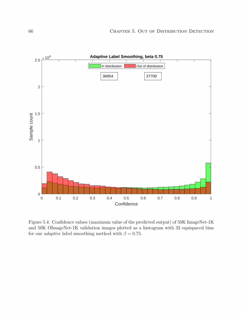
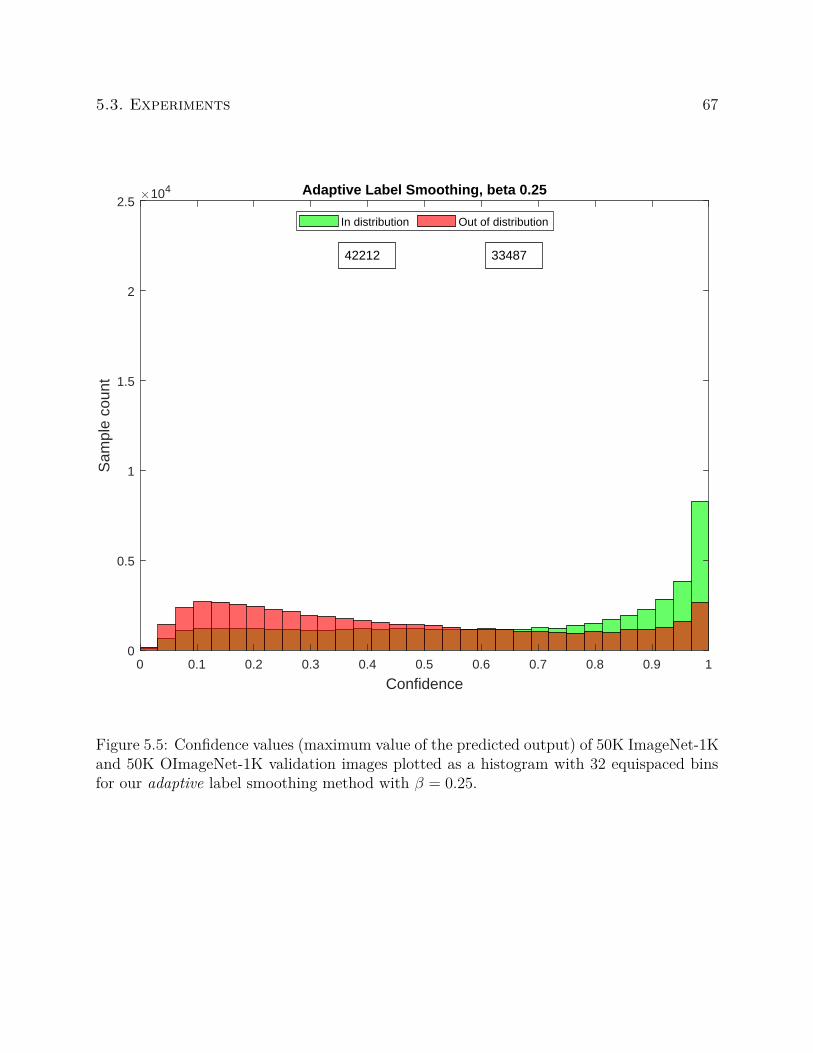
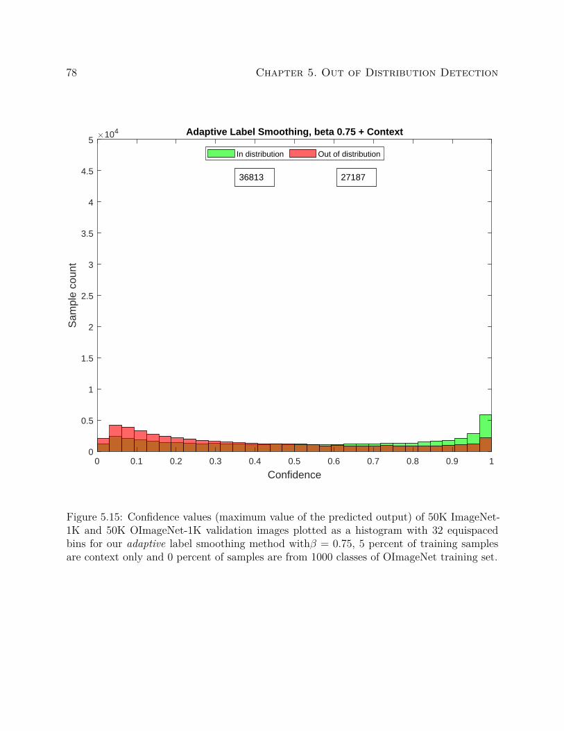
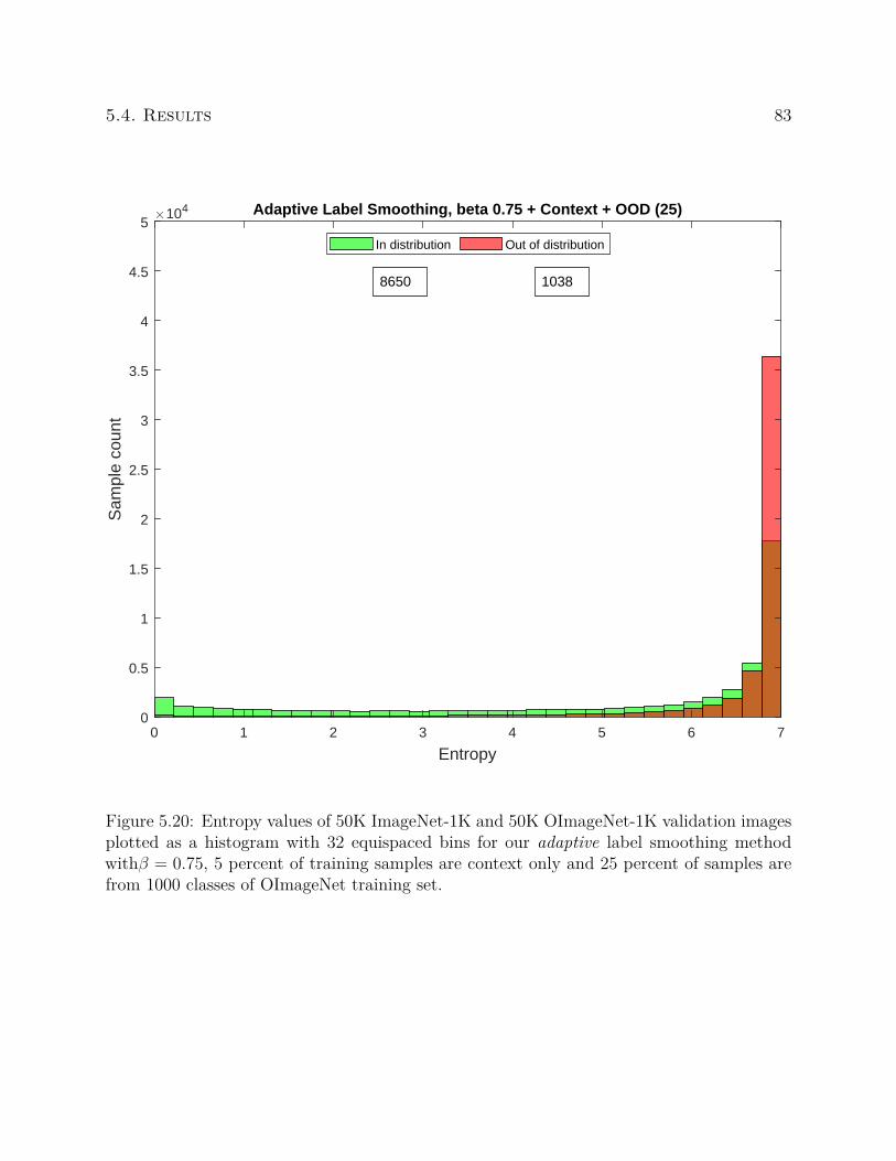
The main contribution of this chapter is that we have developed a novel way to adapt adaptive
label smoothing that was described in the previous chapter for out of distribution detection.
To demonstrate improved out of distribution detection we have trained 14 classifiers and plot
the confidence and entropy histograms over the validation samples.
5.1 Related Work
Classification convolutional neural networks always output in the space of the learnt classes
while predicting the class of a given image regardless of what the image consists of. For
example an ImageNet 1-K trained CNN can not say if the given image has no objects that
it was trained on if it is provided with an image of a dinosaur (not an ImageNet category)
or if the image has the main object cut out of it (context only). To build robustness, many
approaches have been proposed [14, 42, 68]. Our goal is to train with images belonging to
out of distribution and context using soft labels (a uniform distribution of probability over
the set of target classes) for such images. This is a novel way to use soft labels as it allows
the model to learn better confidence bounds.
61
62 Chapter 5. Out of Distribution Detection
5.2 Method
We train classifiers as before in chapter 4, however we validate on novel classes. A good clas-
sifier would produce a low confidence/high entropy prediction when presented with images
from novel (unseen during training) classes. We use the wordnet embeddings to create an
alternative to ImageNet-1K from the larger ImageNet-22K dataset and refer to this dataset
as OImageNet-1K. OImageNet-1K consists of about 800K images in training and 50K images
in validation sets. We refer to the validation set of ImageNet-1K as ‘In distribution’ and the
validation set of OImageNet-1K as ‘Out of distribution’.
We compute entropy based on the information theory definition. Entropy can be used to
measure the uncertainty of the output probability distribution. For a dataset consisting of
K classes and output probability distribution denoted by pi, we can compute entropy per
sample xi using the equation below.
H(xi) = −K∑
i=1pi ln pi (5.1)
5.3 Experiments
We show the confidence histogram plots for each of the models as this is one the standard
approaches for plotting in distribution vs. out of distribution predictions. For the confidence
plots, we compute the bincounts for samples having a confidence value greater than 0.25 and
for the entropy plots we compute bin counts having entropy under 2 natural units (NATs).
5.3. Experiments 63
Hard Label
0 0.1 0.2 0.3 0.4 0.5 0.6 0.7 0.8 0.9 1
Confidence
0
0.5
1
1.5
2
2.5
Sam
ple
coun
t
104
In distribution Out of distribution
47408 42748
Figure 5.1: Confidence values (maximum value of the predicted output) of 50K ImageNet-1Kand 50K OImageNet-1K validation images plotted as a histogram with 32 equispaced bins forthe hard label case. Clearly, there is no distinct way to threshold the different distributionsas they severely overlap with one another.
64 Chapter 5. Out of Distribution Detection
Label Smoothing
0 0.1 0.2 0.3 0.4 0.5 0.6 0.7 0.8 0.9 1
Confidence
0
0.5
1
1.5
2
2.5
Sam
ple
coun
t
104
In distribution Out of distribution
42784 33077
Figure 5.2: Confidence values (maximum value of the predicted output) of 50K ImageNet-1Kand 50K OImageNet-1K validation images plotted as a histogram with 32 equispaced binsfor the standard uniform label smoothing case. The separation is better than the hard labelcase, but there is plenty of overlap.
5.3. Experiments 65
Adaptive Label Smoothing
0 0.1 0.2 0.3 0.4 0.5 0.6 0.7 0.8 0.9 1
Confidence
0
0.5
1
1.5
2
2.5
Sam
ple
coun
t
104
In distribution Out of distribution
31726 23111
Figure 5.3: Confidence values (maximum value of the predicted output) of 50K ImageNet-1Kand 50K OImageNet-1K validation images plotted as a histogram with 32 equispaced binsfor our adaptive label smoothing method. The separation is better than the hard label andlabel smoothing cases, as we produce low confidence scores for a much larger number of outof distribution samples.
66 Chapter 5. Out of Distribution Detection
Adaptive Label Smoothing, beta 0.75
0 0.1 0.2 0.3 0.4 0.5 0.6 0.7 0.8 0.9 1
Confidence
0
0.5
1
1.5
2
2.5
Sam
ple
coun
t
104
In distribution Out of distribution
36954 27700
Figure 5.4: Confidence values (maximum value of the predicted output) of 50K ImageNet-1Kand 50K OImageNet-1K validation images plotted as a histogram with 32 equispaced binsfor our adaptive label smoothing method with β = 0.75.
5.3. Experiments 67
Adaptive Label Smoothing, beta 0.25
0 0.1 0.2 0.3 0.4 0.5 0.6 0.7 0.8 0.9 1
Confidence
0
0.5
1
1.5
2
2.5
Sam
ple
coun
t
104
In distribution Out of distribution
42212 33487
Figure 5.5: Confidence values (maximum value of the predicted output) of 50K ImageNet-1Kand 50K OImageNet-1K validation images plotted as a histogram with 32 equispaced binsfor our adaptive label smoothing method with β = 0.25.
68 Chapter 5. Out of Distribution Detection
Adaptive Label Smoothing + Context + half OOD (5)
0 0.1 0.2 0.3 0.4 0.5 0.6 0.7 0.8 0.9 1
Confidence
0
0.5
1
1.5
2
2.5
Sam
ple
coun
t
104
In distribution Out of distribution
30301 12984
Figure 5.6: Confidence values (maximum value of the predicted output) of 50K ImageNet-1Kand 50K OImageNet-1K validation images plotted as a histogram with 32 equispaced binsfor our adaptive label smoothing method with 5 percent of training samples are context onlyand 5 percent of samples are from 500 classes of OImageNet training set.
5.3. Experiments 69
Adaptive Label Smoothing+ Context + OOD (5)
0 0.1 0.2 0.3 0.4 0.5 0.6 0.7 0.8 0.9 1
Confidence
0
0.5
1
1.5
2
2.5
Sam
ple
coun
t
104
In distribution Out of distribution
30212 11716
Figure 5.7: Confidence values (maximum value of the predicted output) of 50K ImageNet-1Kand 50K OImageNet-1K validation images plotted as a histogram with 32 equispaced binsfor our adaptive label smoothing method with 5 percent of training samples are context onlyand 5 percent of samples are from 1000 classes of OImageNet training set.
As shown in the confidence histogram plots 5.1, 5.2, 5.3, 5.4, 5.5 , 5.6 and 5.7 adaptive
label smoothing helps identify novel classes even though they were never presented during
training. Predictions under a certain threshold can be discarded or communicated to the
70 Chapter 5. Out of Distribution Detection
end user or a safety critical system using our approach. This helps improve precision for real
world applications. We also show similar results with our entropy plots 5.8, 5.9, 5.10, 5.11,
5.12 , 5.13 and 5.14.
Hard Label
0 1 2 3 4 5 6 7
Entropy
0
0.5
1
1.5
2
2.5
Sam
ple
coun
t
104
In distribution Out of distribution
42080 31196
Figure 5.8: Entropy values of 50K ImageNet-1K and 50K OImageNet-1K validation imagesplotted as a histogram with 32 equispaced bins for the hard label case. Clearly, there isno distinct way to threshold the different distributions as they severely overlap with oneanother.
5.3. Experiments 71
Label Smoothing
0 1 2 3 4 5 6 7
Entropy
0
0.5
1
1.5
2
2.5
Sam
ple
coun
t
104
In distribution Out of distribution
30170 15280
Figure 5.9: Entropy values of 50K ImageNet-1K and 50K OImageNet-1K validation imagesplotted as a histogram with 32 equispaced bins for the standard uniform label smoothingcase. The separation is better than the hard label case, but there is plenty of overlap.
72 Chapter 5. Out of Distribution Detection
Adaptive Label Smoothing
0 1 2 3 4 5 6 7
Entropy
0
0.5
1
1.5
2
2.5
Sam
ple
coun
t
104
In distribution Out of distribution
17529 9932
Figure 5.10: Entropy values of 50K ImageNet-1K and 50K OImageNet-1K validation imagesplotted as a histogram with 32 equispaced bins for our adaptive label smoothing method.The separation is better than the hard label and label smoothing cases, as we produce lowEntropy scores for a much larger number of out of distribution samples.
5.3. Experiments 73
Adaptive Label Smoothing, beta 0.75
0 1 2 3 4 5 6 7
Entropy
0
0.5
1
1.5
2
2.5
Sam
ple
coun
t
104
In distribution Out of distribution
21081 11984
Figure 5.11: Entropy values of 50K ImageNet-1K and 50K OImageNet-1K validation imagesplotted as a histogram with 32 equispaced bins for our adaptive label smoothing methodwith β = 0.75.
74 Chapter 5. Out of Distribution Detection
Adaptive Label Smoothing, beta 0.25
0 1 2 3 4 5 6 7
Entropy
0
0.5
1
1.5
2
2.5
Sam
ple
coun
t
104
In distribution Out of distribution
30297 17387
Figure 5.12: Entropy values of 50K ImageNet-1K and 50K OImageNet-1K validation imagesplotted as a histogram with 32 equispaced bins for our adaptive label smoothing methodwith β = 0.25.
5.3. Experiments 75
Adaptive Label Smoothing + Context + half OOD (5)
0 1 2 3 4 5 6 7
Entropy
0
0.5
1
1.5
2
2.5
Sam
ple
coun
t
104
In distribution Out of distribution
16795 4675
Figure 5.13: Entropy values of 50K ImageNet-1K and 50K OImageNet-1K validation imagesplotted as a histogram with 32 equispaced bins for our adaptive label smoothing methodwith 5 percent of training samples are context only and 5 percent of samples are from 500classes of OImageNet training set.
76 Chapter 5. Out of Distribution Detection
Adaptive Label Smoothing+ Context + OOD (5)
0 1 2 3 4 5 6 7
Entropy
0
0.5
1
1.5
2
2.5
Sam
ple
coun
t
104
In distribution Out of distribution
16660 3833
Figure 5.14: Entropy values of 50K ImageNet-1K and 50K OImageNet-1K validation imagesplotted as a histogram with 32 equispaced bins for our adaptive label smoothing methodwith 5 percent of training samples are context only and 5 percent of samples are from 1000classes of OImageNet training set.
5.4. Results 77
5.4 Results
To further understand the effect of increasing the fraction(5 percent being used in 5.6 and
5.7) of out of distribution samples (with uniform smooth labels) we train classifiers with
β = 0.75 with different amounts of out of distribution samples supplied per training epoch.
For the confidence plots, we compute the bincounts for samples having a confidence value
greater than 0.25 and for the entropy plots we compute bin counts having entropy under 2
natural units (NATs).
78 Chapter 5. Out of Distribution Detection
Adaptive Label Smoothing, beta 0.75 + Context
0 0.1 0.2 0.3 0.4 0.5 0.6 0.7 0.8 0.9 1
Confidence
0
0.5
1
1.5
2
2.5
3
3.5
4
4.5
5
Sam
ple
coun
t
104
In distribution Out of distribution
36813 27187
Figure 5.15: Confidence values (maximum value of the predicted output) of 50K ImageNet-1K and 50K OImageNet-1K validation images plotted as a histogram with 32 equispacedbins for our adaptive label smoothing method withβ = 0.75, 5 percent of training samplesare context only and 0 percent of samples are from 1000 classes of OImageNet training set.
5.4. Results 79
Adaptive Label Smoothing, beta 0.75 + Context
0 1 2 3 4 5 6 7
Entropy
0
0.5
1
1.5
2
2.5
3
3.5
4
4.5
5
Sam
ple
coun
t
104
In distribution Out of distribution
21101 11835
Figure 5.16: Entropy values of 50K ImageNet-1K and 50K OImageNet-1K validation imagesplotted as a histogram with 32 equispaced bins for our adaptive label smoothing methodwithβ = 0.75, 5 percent of training samples are context only and 0 percent of samples arefrom 1000 classes of OImageNet training set.
Figure 5.17: Confidence values (maximum value of the predicted output) of 50K ImageNet-1K and 50K OImageNet-1K validation images plotted as a histogram with 32 equispacedbins for our adaptive label smoothing method withβ = 0.75, 5 percent of training samplesare context only and 5 percent of samples are from 1000 classes of OImageNet training set.
Figure 5.18: Entropy values of 50K ImageNet-1K and 50K OImageNet-1K validation imagesplotted as a histogram with 32 equispaced bins for our adaptive label smoothing methodwithβ = 0.75, 5 percent of training samples are context only and 5 percent of samples arefrom 1000 classes of OImageNet training set.
Figure 5.19: Confidence values (maximum value of the predicted output) of 50K ImageNet-1K and 50K OImageNet-1K validation images plotted as a histogram with 32 equispacedbins for our adaptive label smoothing method withβ = 0.75, 5 percent of training samplesare context only and 25 percent of samples are from 1000 classes of OImageNet training set.
Figure 5.20: Entropy values of 50K ImageNet-1K and 50K OImageNet-1K validation imagesplotted as a histogram with 32 equispaced bins for our adaptive label smoothing methodwithβ = 0.75, 5 percent of training samples are context only and 25 percent of samples arefrom 1000 classes of OImageNet training set.
Figure 5.21: Confidence values (maximum value of the predicted output) of 50K ImageNet-1K and 50K OImageNet-1K validation images plotted as a histogram with 32 equispacedbins for our adaptive label smoothing method withβ = 0.75, 5 percent of training samplesare context only and 5 percent of samples are from 500 classes of OImageNet training set.
Figure 5.22: Entropy values of 50K ImageNet-1K and 50K OImageNet-1K validation imagesplotted as a histogram with 32 equispaced bins for our adaptive label smoothing methodwithβ = 0.75, 5 percent of training samples are context only and 5 percent of samples arefrom 500 classes of OImageNet training set.
Figure 5.23: Confidence values (maximum value of the predicted output) of 50K ImageNet-1K and 50K OImageNet-1K validation images plotted as a histogram with 32 equispacedbins for our adaptive label smoothing method withβ = 0.75, 5 percent of training samplesare context only and 25 percent of samples are from 500 classes of OImageNet training set.
Figure 5.24: Entropy values of 50K ImageNet-1K and 50K OImageNet-1K validation imagesplotted as a histogram with 32 equispaced bins for our adaptive label smoothing methodwithβ = 0.75, 5 percent of training samples are context only and 25 percent of samples arefrom 500 classes of OImageNet training set.
Figure 5.25: Confidence values (maximum value of the predicted output) of 50K ImageNet-1K and 50K OImageNet-1K validation images plotted as a histogram with 32 equispacedbins for our adaptive label smoothing method withβ = 0.75, 5 percent of training samplesare context only and 50 percent of samples are from 500 classes of OImageNet training set.
Figure 5.26: Entropy values of 50K ImageNet-1K and 50K OImageNet-1K validation imagesplotted as a histogram with 32 equispaced bins for our adaptive label smoothing methodwithβ = 0.75, 5 percent of training samples are context only and 50 percent of samples arefrom 500 classes of OImageNet training set.
Figure 5.27: Confidence values (maximum value of the predicted output) of 50K ImageNet-1K and 50K OImageNet-1K validation images plotted as a histogram with 32 equispacedbins for our adaptive label smoothing method withβ = 0.75, 5 percent of training samplesare context only and 75 percent of samples are from 500 classes of OImageNet training set.
Figure 5.28: Entropy values of 50K ImageNet-1K and 50K OImageNet-1K validation imagesplotted as a histogram with 32 equispaced bins for our adaptive label smoothing methodwithβ = 0.75, 5 percent of training samples are context only and 75 percent of samples arefrom 500 classes of OImageNet training set.
As we show in figures 5.15, 5.16, 5.17, 5.18, 5.19, 5.20, 5.21, 5.22, 5.23, 5.24, 5.25, 5.26, 5.27
and 5.28 the increase in the fraction of out of distribution samples supplied during training
increases the proportion of in distribution samples after thresholding. However, the overall
92 Chapter 5. Out of Distribution Detection
number of samples drops drastically, this also results in an accuracy drop on the target
dataset (in distribution). In the case of figure 5.15 the mean accuracy on the in distribution
dataset is 68.1 percent, for figure 5.17 the accuracy is 67.7 percent and for figure 5.19 the
accuracy is 62 percent. In the case of figure 5.27, the mean accuracy dropped to 47 percent.
5.5 Conclusion
This work has addressed the problems of out of distribution detection using a novel approach
called adaptive label smoothing. Our approach helps train classifiers that pay attention to
the more discriminative regions and learn to recognize out of distribution images better than
standard hard label or label smoothing approaches. Our approach can be used to produce
high entropy predictions when context-only or out of distribution images are provided as
input to the classifier.
Chapter 6
Conclusions
The tremendous growth in the field of machine learning in the past two decades can be
attributed to high accuracies and widespread real-world deployment of the models trained
using large public datasets like ImageNet. Even though the modern day machine learning
models have shown great improvement in performance, they suffer from a myriad of problems.
Some of the problems commonly seen are poor generalization, overconfidence and poor out
of distribution performance. These problems can be attributed to the datasets being used,
algorithms being used to train and the model architectures as well. In this dissertation we
developed approaches to mitigate some of the problems pertaining to bias, overconfidence
and out of distribution detection.
Specifically, in Chapter 3 we developed an augmentation approach that is able to use bound-
ing box information and augment data on the fly. This approach provides control over
scale, size and position over multiple objects and maintains the class context at the same
time. This is the first approach that ever utilized bounding box information to augment
classifiers trained on ImageNet 1-K. In tests with ImageNet 1-K dataset, our approach when
combined with CutMix using the ResNet-50 architecture outperforms the standard baseline
by 1.8 percent. After fine tuning on the challenging MS-COCO, using Faster R-CNN with
a ResNet-50 backbone, our approach when combined with CutMix yielded a performance of
32.3 mAP, which is an improvement of 0.5 mAP when just CutMix was used for the classifier
regularization.
93
94 Chapter 6. Conclusions
Chapter 4 addresses the algorithmic deficiencies in modern day image classifiers using a novel
approach called adaptive label smoothing. We produce class probabilities that are grounded
in the spatial footprint of the object being classified. This approach is novel and has a posi-
tive impact in improving the localization ability of the classifiers. Our approach also results
in better interpretability of the outputs produced by the CNNs and reduces the overconfi-
dence score. That is, we encourage our model to produce high entropy predictions on images
that barely contain any relevant objects. When compared to other baseline approaches on
ImageNet 1-K, our approaches produce the lowest overconfidence scores. After fine tuning on
the challenging MS-COCO, using Faster R-CNN with a ResNet-50 backbone, our approach
matches the performance of CutMix in terms of mAP. Our approach provides lower overcon-
fidence scores and improved localization at the same time. Our confidences/predictions are
based on the size of an object and we are over the diagonal because of this (under the diag-
onal is undesirable). We are more accurate than we are confident compared to all baselines
as we show using reliability charts in figure 4.7. The average objectness of images in the
validation set of ImageNet is 0.49 and the mean confidence of our approach is 0.60 compared
to the mean confidence of 0.86 using the hard label approach. The mean deviation computed
as the mean of the absolute difference between confidence and objectness for the hard label
case is 0.42 and for our approach is 0.24. Using these metrics we show that our confidences
are explainable as they closely match the objectness statistics much better, our predictions
are explainable and we ground our labels/confidences in the object size as opposed to making
correct predictions using contextual information only as shown in table 4.1.
Lastly, Chapter 5 extends the techniques developed in Chapter 4 to improve the out of
distribution of CNNs. We supply images belonging to novel unseen classes during training,
but provide a vector with a uniform probability distribution over all classes as the label
for all of them. That is, we encourage our model to produce high entropy predictions on
95
unseen categories. Using bin counts we show that our approach is better and rejecting out of
distribution samples when the confidence is thresholded at values over 0.25 and the entropy
is thresholded under 2.
Bibliography
[1] Bogdan Alexe, Thomas Deselaers, and Vittorio Ferrari. Measuring the objectness of
image windows. IEEE Transactions on Pattern Analysis and Machine Intelligence
(TPAMI), 34(11):2189–2202, 2012.
[2] Dario Amodei, Chris Olah, Jacob Steinhardt, Paul F. Christiano, John Schulman, and
Dan Mané. Concrete problems in AI safety. arXiv preprint arXiv:1606.06565, 2016.
[3] Lisa Anne Hendricks, Kaylee Burns, Kate Saenko, Trevor Darrell, and Anna Rohrbach.
Women also snowboard: Overcoming bias in captioning models. In Proceedings of the
European Conference on Computer Vision (ECCV), pages 771–787, 2018.
[4] Jimmy Ba and Rich Caruana. Do deep nets really need to be deep? In Advances in
Neural Information Processing Systems, pages 2654–2662, 2014.
[5] Peter W Battaglia, Jessica B Hamrick, Victor Bapst, Alvaro Sanchez-Gonzalez, Vinicius
Zambaldi, Mateusz Malinowski, Andrea Tacchetti, David Raposo, Adam Santoro, Ryan
Faulkner, et al. Relational inductive biases, deep learning, and graph networks. arXiv
preprint arXiv:1806.01261, 2018.
[6] Aditya Chattopadhay, Anirban Sarkar, Prantik Howlader, and Vineeth N Balasubra-
manian. Grad-cam++: Generalized gradient-based visual explanations for deep con-
volutional networks. In 2018 IEEE Winter Conference on Applications of Computer
Vision (WACV), pages 839–847. IEEE, 2018.
[7] Junsuk Choe and Hyunjung Shim. Attention-based dropout layer for weakly supervised
96
BIBLIOGRAPHY 97
object localization. In Proceedings of the IEEE Conference on Computer Vision and