Wayne State University Digital Commons@Wayne State University Wayne State University Dissertations 1-1-2012 Reliability and effect of partially restrained wood shear walls John Joseph Gruber Wayne State University, [email protected]is Open Access Dissertation is brought to you for free and open access by Digital Commons@Wayne State University. It has been accepted for inclusion in Wayne State University Dissertations by an authorized administrator of Digital Commons@Wayne State University. For more information, please contact [email protected]. Recommended Citation Gruber, John Joseph, "Reliability and effect of partially restrained wood shear walls" (2012). Wayne State University Dissertations. Paper 442. hp://digitalcommons.wayne.edu/oa_dissertations/442
Transcript
Wayne State UniversityDigital Commons@Wayne State University
Wayne State University Dissertations
1-1-2012
Reliability and effect of partially restrained woodshear wallsJohn Joseph GruberWayne State University, [email protected]
This Open Access Dissertation is brought to you for free and open access by Digital Commons@Wayne State University. It has been accepted forinclusion in Wayne State University Dissertations by an authorized administrator of Digital Commons@Wayne State University. For more information,please contact [email protected].
Recommended CitationGruber, John Joseph, "Reliability and effect of partially restrained wood shear walls" (2012). Wayne State University Dissertations. Paper442.http://digitalcommons.wayne.edu/oa_dissertations/442
Figure 26: Data Acquisition Software Graphics Display ............................................. 158
Figure 27: Actuator Control Software Load Steps ...................................................... 159
xiii
LIST OF GRAPHS
Graph 1: Effect of Uplift Restraint on the Lateral Load Capacity of a Shear Wall Based on Mechanics-Based Approach (Ni and Karacabeyli 2000) .......................... 24
Graph 2: Effect of Uplift Restraint on the Lateral Load Capacity of a Shear Wall Based on Empirical Approach (Ni and Karacabeyli 2000) ........................................ 25
Graph 3: Nail Deformation Model................................................................................. 42
Graph 4: Probability Density Function of Shear Wall Load........................................... 44
Graph 5: Failure Region of PDF of Shear Wall Load.................................................... 45
Graph 6: Reliability Index, β, on the Standard Normal Distribution............................... 46
Graph 7: Hysteresis Curve for Wall A1......................................................................... 57
Graph 8: Summary of Wall Tests ................................................................................. 58
Graph 9: 8d Common Nail Curves from Wall Group A.................................................. 59
Graph 10: 8d Common Nail Curve Model .................................................................... 60
Graph 11: Hold down Stiffness from Test Results........................................................ 62
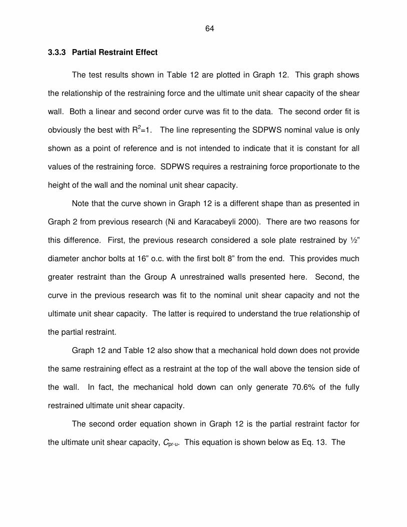
Graph 12: Partial Restraint Effect on Strength ............................................................. 65
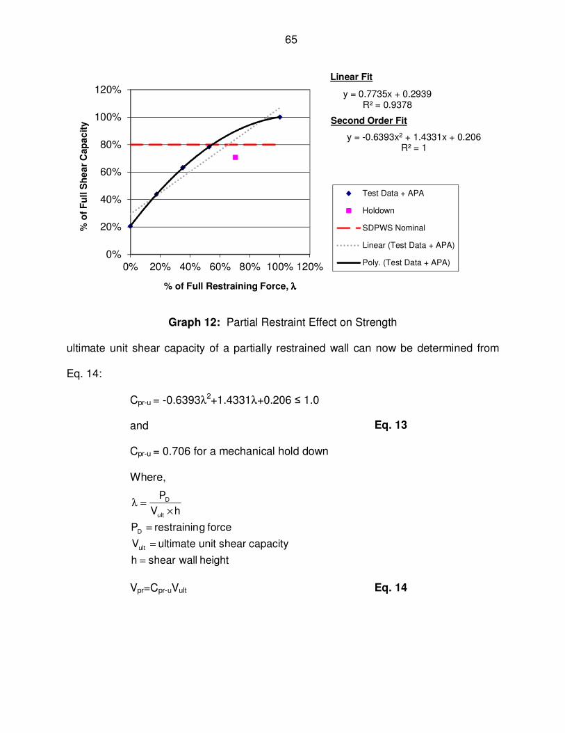
Graph 13: Unit Shear Capacity of Wall A on Normal Probability Paper........................ 66
Graph 14: Unit Shear Capacity of Wall A on Log-Normal Probability Paper ................ 67
Graph 15: Correlation of Wall Strength to Specific Gravity........................................... 70
Graph 16: Sheathing Nail Data for ABAQUS ............................................................... 80
Graph 17: 16d Stud Withdrawal Nail Data for ABAQUS............................................... 82
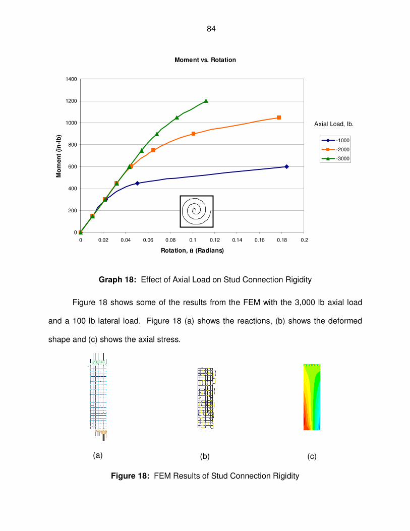
Graph 18: Effect of Axial Load on Stud Connection Rigidity ........................................ 84
Graph 19: Hold Down Stiffness for ABAQUS ............................................................... 86
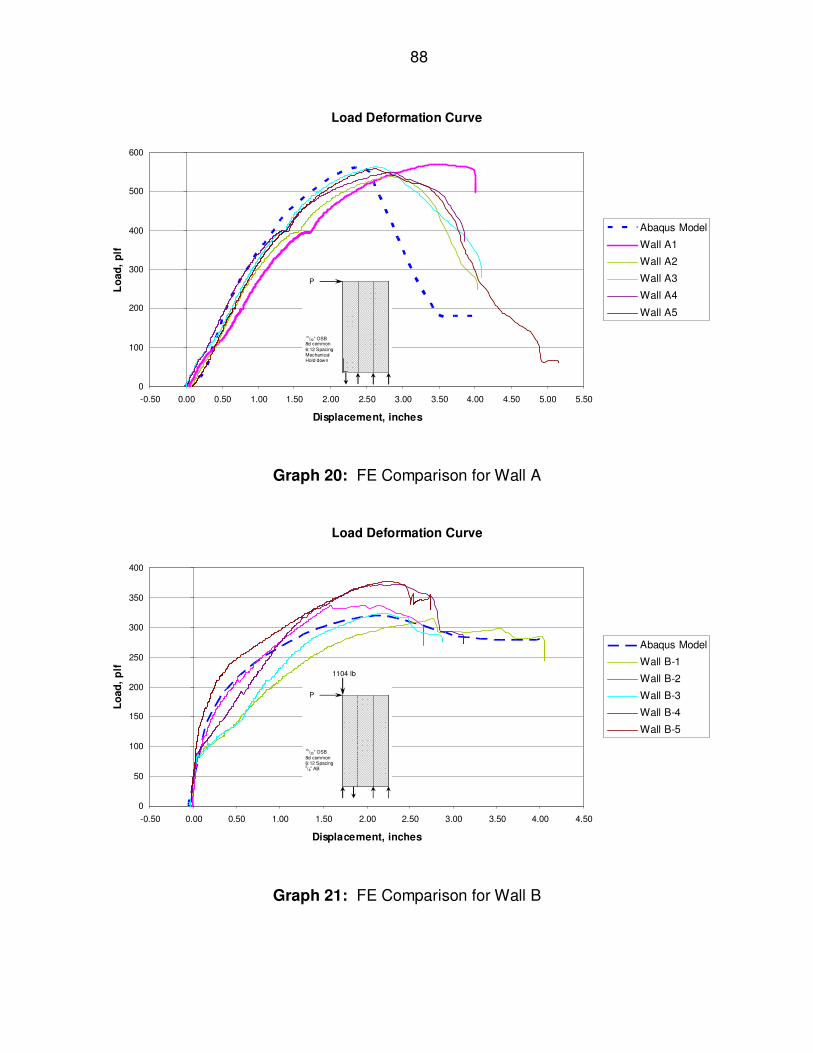
Graph 20: FE Comparison for Wall A........................................................................... 88
Graph 21: FE Comparison for Wall B........................................................................... 88
xiv
Graph 22: FE Comparison for Wall C........................................................................... 89
Graph 23: FE Comparison for Wall D........................................................................... 89
Graph 24: FE Comparison for Wall E........................................................................... 90
Graph 25: FE Model of Fully Restrained wall Compared to FE Model of Walls A-E .... 90
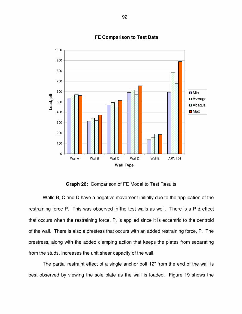
Graph 26: Comparison of FE Model to Test Results.................................................... 92
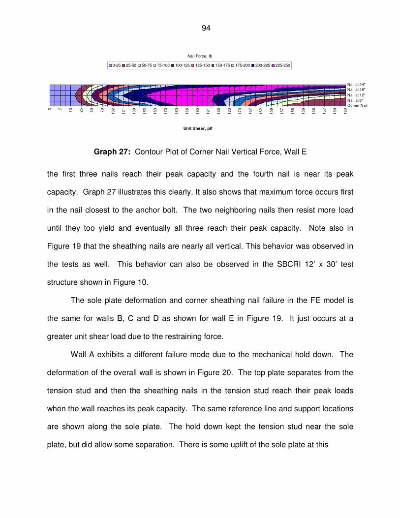
Graph 27: Contour Plot of Corner Nail Vertical Force, Wall E...................................... 94
Graph 28: Calibration of Unrestrained Shear Wall ..................................................... 106
Graph 29: Partial Restraint Effect on Strength - Calibrated......................................... 107
Graph 30: Comparison of Calibrated Partial Restraint Effect ..................................... 108
Graph 31: Partial Restraint Effect, ASD, without Specific Gravity .............................. 121
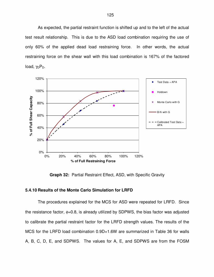
Graph 32: Partial Restraint Effect, ASD, with Specific Gravity ................................... 125
Graph 33: Partial Restraint Effect, LRFD, without Specific Gravity ............................ 127
Graph 34: Partial Restraint Effect, LRFD, with Specific Gravity ................................. 130
Graph 35: Comparison of Partial Restraint................................................................. 136
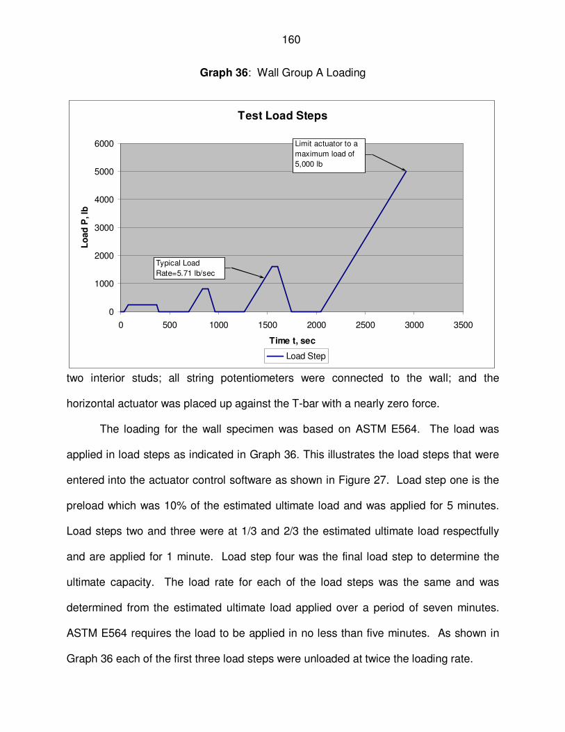
Graph 36: Wall Group A Loading ............................................................................... 160
Graph 37: Distribution of the Specific Gravity for SPF-S Studs.................................. 165
Graph 38: Distribution of the Specific Gravity for OSB Sheathing.............................. 166
xv
LIST OF TABLES
Table 1: Historic House Data (HUD 2001) ..................................................................... 5
Table 2: Current Construction Methods (HUD 2001)...................................................... 6
Table 41: Test Equipment ........................................................................................... 156
Table 42: Chi-Square Test for Specific Gravity Probability Distribution for Studs ...... 165
Table 43: Specific Gravity of Members in Wall Group A............................................. 167
Table 44: Specific Gravity of Members in Wall Group B............................................. 167
xvii
Table 45: Specific Gravity of Members in Wall Group C ............................................ 168
Table 46: Specific Gravity of Members in Wall Group D ............................................ 168
Table 47: Specific Gravity of Members in Wall Group E............................................. 169
1
CHAPTER 1
INTRODUCTION
The purpose of this research is to examine the reliability levels of the prescriptive
wall bracing requirements of the 2009 International Residential Code (IRC) and the
engineered shear wall requirements of the 2009 International Building Code (IBC) along
with the 2005 Special Design Provisions for Wind and Seismic (AF&PA SDPWS). This
research encompasses structures constructed in 90 m.p.h. wind areas with exposure B.
In order to understand the focus of the proposed research, it is necessary to
understand the history of housing, housing construction practices, and wall bracing.
Based upon the ASCE 7 wind speed map shown in Figure 1, this research affects the
majority of the housing in the continental United States since it applies to structures in
low wind speed and low seismic areas. Currently, a prescriptive design method is
dominant for the design of lateral bracing for single family houses. When the limits of
the prescriptive design are exceeded, then an engineered alternative is necessary.
Based on the information available today, the reliability levels of these two design
methods are not equivalent. It is desirable to understand the reliability levels of these
two systems and compare them.
The reliability analysis is useful for several reasons. First, it provides a
comparison of the two design philosophies in a way that is independent of the design
methods by using the second-moment reliability index β. This “provides a relative
Figure 1: Continental US Shaded Wind Speed Map (WBDG 2010)
90 MPH or Less
Reprinted with permission from the Whole Building Design Guide National Institute of Builidng Sciences.
2
3
measure of the safety of a structural component or system and serves as the
cornerstone of code calibration studies” (van de Lindt and Rosowsky 2005). Second,
the study is useful to calibrate resistance factors to unify the two design methods with
respect to structural safety. This is beneficial for alternate building materials and
systems that could provide economic, energy or sustainability benefits.
This research provides the following items:
1. The reliability index of the unit shear capacity for 15/32” Wood Structural
Panels (WSP) in SDPWS (2005)
2. The appropriateness of ASTM E72 for walls anchored with mechanical
hold downs and partially restrained IRC (2009) prescriptive walls.
3. Verification for the resistance factor used by the SDPWS.
4. Recommended codified nominal unit shear design values for wind load
for unrestrained shear walls constructed in accordance with the 2009
IRC using 15/32” WSP.
5. Recommended codified nominal unit shear design values for wind load
for fully restrained shear walls constructed in accordance with the 2009
IRC using 15/32” WSP.
6. Proposed requirement for unrestrained shear wall tests for WSP
manufacturers in the Voluntary Product Standard PS 2-04 titled
Performance Standards for Wood-Based Structural-Use Panels (NIST
2004) for WSP.
4
7. Recommended IRC utilization of the unrestrained shear wall nominal
unit shear design values or definition of some minimum restraining
force to be known present.
The above results will create an equitable design methodology between the IRC
prescriptive method and the SDPWS. When implemented and utilized in the IRC,
alternate products and engineered alternatives can be provided without the appearance
of over-conservatism.
1.1 History
1.1.1 Historic House Data
The total load resistance of wall bracing in houses is not only dependent upon
the material, but also the spacing of brace wall lines and aspect ratios of brace walls.
The spacing of the brace wall lines obviously affects the tributary wind area of each
brace wall line. The aspect ratios typically affect the strength and certainly affect the
stiffness of the brace walls. Therefore, the number of openings in a wall as well as the
height of a wall can affect the load resistance of the lateral load resisting system. These
geometric features have been changing during the past century, creating a greater
demand on lateral bracing systems.
Beyond the structural history of brace walls, the economic value of homes is also
of concern. As the value of homes increase, the financial risk due to wind damage also
increases.
5
Table 1 shows a comparison of house construction over the 20th century. The
average size of houses more than doubled in this period of time, while the number of
bedrooms remained about the same. Today’s homes include more large open spaces
than homes built in the early 1900s. Over the same time period, housing costs have
increased by a factor of 100. The inflation-adjusted housing cost in the early 1900s was
about $35.00/sq. ft. The cost in 2000 was about $100.00/sq. ft.
Table 1: Historic House Data (HUD 2001)
Early 1900’s Mid 1900’s Late 1900’s
Population 76 Million (40% urban, 60% rural)
150 Million (64 % urban, 36% rural)
270 Million (76% urban, 24% rural)
Median Family Income $490 $3,319 $45,000 New Home Price Average Unknown
1 $11,000 $200,000
Type of Purchase Typically Cash FHA Mortgage, 4.25% (few options)
8% (many options)
Ownership Rate 46 % 55% 67% Total Housing Units 16 Million 43 Million 107 Million (approx. 50%
single-family) Number of annual housing starts
189,000 (65% single-family)
1.95 Million (85% single-family)
1.54 Million (approx. 50% single family)
Average Size (starts) < 1,000 sq. ft. 1,000 sq. ft. 2,000 sq. ft. or more Stories 1 to 2 1 (86%); 2 or more
(14%) 1 (48%); 1½ or 2 (49%)
Bedrooms 2 to 3 2 (66%); 3 (33%) 2 or less (12%); 3 (54%); 4 or more (34%)
Bathrooms 0 or 1 1½ or less (96%) 1½ or less (7%); 2 (40%); 2½ + (53%)
Garage 1 car (41%); 0 (53%) 2 car (65%)
Table 1 also indicates that there has been a large movement to urban settings
from rural. The shift from rural to urban settings indicates that wind exposure is
decreasing as the exposure category is B for urban locations and typically C for rural
locations (ASCE 7-05).
1 Based on “Housing at the Millennium: Facts, Figures, and Trends,” the average new home cost was less
than $5,000. However, this estimate is potentially skewed in that many people could not afford a “house” of the nature considered in the study. Based on Sears, Roebuck, and Co. catalogue prices at the turn of the century, a typical house may have ranged from $1,000 to $2,000, including land.
6
Construction methods for housing have also changed throughout the 20th
century. A summary of the current construction methods for 2001 is presented in Table
2. Of interest for this research are the foundation type, wall sheathing and wall framing.
The dominant foundation type is a slab on grade system. This system includes
perimeter footings, typically to frost depth; interior footings at interior-bearing locations;
and a floor slab constructed on grade. The dominant wall sheathing is oriented strand
board (OSB) with foam panels used in 24% of the construction. The foam panels are
typically non-structural sheathing. The dominant wall framing is 2x4 studs at 16” o.c.
This research considers slab on grade construction, OSB intermittent sheathing, and
2x4 stud wall framing at 16” o.c.
Table 2: Current Construction Methods (HUD 2001)
Foundation Type Basement (34%); Crawlspace (11%); Slab (54%) Floor Framing Type: Lumber (62%); Wood Trusses (9%); Wood I-joists (28%)
Size of Lumber: 2x8 (8%); 2x10 (70%); 2x12 (21%) Type of Lumber: SYP (39%); DF (23%); other (37%)
area on average) Roof Sheathing Plywood (27.6%); OSB (71%) Roof Framing Rafters (6%); I-joists (29%); Wood Trusses (65%) Roof Pitch 4/12 or less (7%); 5/12 to 6/12 (63%); 7/12 or greater (30%) Roof Shape Gable (63%); Hip (36%) Note: Percentages for floor, wall, and roof sheathing and framing are based on total aggregated floor and wall area for housing starts. Other values are given as a percentage of housing starts.
1.1.2 Historic Wall Bracing
Wall bracing in houses to provide lateral stability has evolved over the past
century as framing methods changed from balloon to platform framing and as materials
other than sawn boards and plaster became available. Bracing methods in the early
1900s consisted of no bracing, 1x4 let-in bracing, or horizontal or diagonal wood
7
sheathing (HUD 2001). The method of no bracing apparently relied on the interior wood
lath and plaster for the bracing system.
As early as 1929 the Forest Products Laboratory began comparison testing of
various bracing methods (HUD 2001). The walls tested were 9’ x 14’ and
7’-4” x 12’ with enough vertical restraint to prevent over-turning. These walls were
either solid, had one window opening, or had one window and one door opening. The
results of the tests are presented in (HUD 2001).
1.1.3 Prescriptive Code History
Plywood was introduced in the mid 1900s. This renewed the interest in bracing
methods. Plywood is typically manufactured in 4’ x 8’ sheets and is installed either
continuously over the exterior walls or intermittently. Until the early 2000s, with the
introduction of the International Codes (a combination of the BOCA, UBC, and SBC),
the primary bracing methods in the late 1900s were metal T-bracing, wood structural
panels (plywood or OSB), or gypsum.
Table 1 shows that houses are larger, but don’t have more rooms, therefore
houses have larger rooms today than they did a century ago. This, coupled with larger
window and door openings, has led to less lateral resistance in houses. Although
typically discounted, interior partitions provide additional strength and stiffness to the
lateral resisting system of houses. The percentage of interior partitions in comparison
to floor area has decreased with the increased house size and especially with the large
open spaces enjoyed in the later part of the 1900s. Table 3 summarizes the change in
the amount of interior walls from early last century to late last century. Note that there is
8
a 1.1% and 1.7% reduction in interior walls, as a percent of floor area, for the second
and first floor of two-story houses respectively.
Table 3: Interior Wall Amounts (HUD 2001) (Lineal feet as a percent of floor area of story)
OLDER HOMES (early 1900s)1 MODERN HOMES (late 1900s)2
1 Story 9% ± 1% 1st Floor of 1 to 2 Story 4.3% ± 1% 1st Floor of 2 Story 6% ± 1% 2nd Floor of 2 Story 7.9% ± 1%
2nd Floor of 2 Story 9% ± 1.5% Notes: 1Values based on a small sample of traditional house plans in Sears Catalogues (1910-1926) including
affordable and more expensive construction of 1 and 2 stories. 2Values based on a small sample of representative modern home plans (1990s) including economy
and move-up construction (no luxury homes).
By the late 1900s, Hurricane Andrew and the Northridge Earthquake had
highlighted the importance of lateral bracing in houses. This timing, along with the
development of the International Codes, changed the bracing methods used in
prescriptive design. Much research of wood shear walls and bracing methods focused
on seismic design and cyclic testing. As a result, the codes began prescribing more
lateral bracing.
The current IRC (IRC 2009) uses more of a rational design method to prescribe
wall bracing to resist wind loads than previous editions but varies greatly from the
typical rational (engineered) design method using the ASCE 7-05 and the SDPWS. The
current IRC (IRC 2009) has also made an attempt to utilize both partial wall restraint
and a whole house effect. It is the goal of this research to compare the reliability of the
prescriptive design with the rational design using SDPWS.
9
1.2 Reliability Analysis
1.2.1 Testing
As part of this research, (25) 4’ x 8’ brace walls were monotonically load tested.
These walls varied from full restraint (a mechanical hold down device) to unrestrained
(only a single anchor bolt). The testing was performed at the Structural Building
Components Research Institute located in Madison, WI. The goal of the testing was to
understand the load-deflection behavior and ultimate strength of the varying restraint
conditions and the variability of the ultimate strength.
1.2.2 Verification of Empirical Partial Restraint Factor
The test data was used to verify the empirical partial restraint factor previously
developed by Ni and Karacabeyli (2000). This factor is intended to predict the capacity
of an unrestrained or partially restrained shear wall using the nominal unit shear
strength of a fully restrained wall. Differences between the IRC prescriptive sole plate
anchorage and the anchorage used to develop the empirical partial restraint factor
necessitate a verification of this factor for the IRC wall.
1.2.3 Reliability Model
Using the test results from the 25 tests, ultimate strengths and variability were
used in a first order second moment reliability model (FOSM) and Monte Carlo
Simulation (MCS) to determine the reliability index, β, for the current SDPWS nominal
unit shear strength and the nominal unit shear strength used in the 2009 IRC. The tests
results were also used to identify the random variables used in the reliability model.
10
The reliability analysis used both numerical analysis and Monte Carlo simulation to
evaluate the model.
Once the model was constructed for the varying wall restraint conditions, two
items were varied to provide a target value for β (3.25) for each of these conditions
which is similar to the current reliability index of 3.27 for the SDPWS nominal values.
These items included the resistance factor, φ, and the nominal tabulated unit shear
values for the varying cases.
1.3 Recommendations for Code Revisions
The conclusions of this research include recommendations for code revisions for
unrestrained, partially restrained, and fully restrained shear walls constructed with WSP
with 8d common nails and recommendations for finite element models. These are
based on a 4’x8’ WSP shear wall. The following is a list of these conclusions.
1. The reliability index of the SDPWS nominal unit shear value for 15/32” WSP
was determined using the allowable stress design (ASD) reduction factor and
resistance factor, φ, and APA Research Report 154 (APA 2004).
2. The use of ASTM E72 is inappropriate to determine nominal unit shear design
values.
3. Present nominal unit shear values published in SDPWS cannot be achieved
with a mechanical hold down at the base of the wall.
4. Using reliability analysis for calibration, partial restraint modification factors
are determined for both mechanical hold downs and a dead load restraining
force. These modification factors will be used to modify the nominal unit
11
shear capacity values in SDPWS. These modification factors are presented
for both allowable stress design (ASD) and load and resistance factored
design (LRFD) methods.
5. For equitable designs providing the same level of safety, the IRC 2009 should
publish the required dead load restraining force to achieve the unit shear
design value used. This restraining force should be clearly stated as a design
requirement for the use of the prescriptive method.
6. Finite element models should always include the effect of the boundary
conditions, restraining force, and the connection behavior of the studs-to-
top/sole-plate connections.
1.4 Organization of Thesis
Chapter 2 provides a literature review of codes and standards applicable to this
thesis; previous research regarding partially restrained wood shear walls; finite element
modeling; and reliability studies. The background of the prescriptive wall bracing
methods, design philosophy, and engineered alternate design methods are reviewed to
provide the reader with a basis for this thesis. Finite element modeling methods, nail
strength and load deformation modeling, as well as the nail yield limit theory are
reviewed. A reliability analysis of wood shear walls with wind loads conducted by van
de Lindt is also presented.
In Chapter 3 a summary of the wood shear wall testing conducted is presented.
This includes a brief overview of both ASTM E72 and E564. Summary of data obtained
from the test program that is used for both the finite element modeling and the reliability
study is presented here.
12
In Chapter 4 a finite element model is presented. This model includes a non-
linear finite element model created to simulate the behavior of partially restrained wood
shear walls and shear walls restrained with a mechanical hold down. This model
utilizes nonlinear orthogonal spring pairs using data obtained from the tests conducted.
Results from the finite element model are presented at the end of CHAPTER 4.
In Chapter 5, a systematic reliability analysis is presented. This analysis
concludes with a Monte Carlo simulation including four random variables: wind load,
dead load, wall unit shear capacity, and specific gravity. A partial restraint factor was
developed by calibrating the bias factor with the M-C simulation so that a constant
reliability index of 3.25 is obtained for all restraint conditions for the 4’x 8’ wood shear
wall.
A discussion regarding the intent and use of both ASTM E72 and E564 is
presented in Chapter 6. This describes the limitations of ASTM E72 and the
appropriateness of its use for determining design values.
Conclusions of this thesis are presented in Chapter 7. A brief summary of this
thesis is included here as well as suggestions for future research. The calibrated partial
restraint factors for both allowable stress design (ASD) and load and resistance factored
design (LRFD) are summarized.
13
CHAPTER 2
LITERATURE REVIEW
In this chapter a general introduction is given to the current design requirements
for intermittent brace walls in residential construction, a review of previous reliability
studies, a review of previous finite element modeling methods, and a review of recent
IRC wall testing. Specifically, the prescriptive requirements of the 2009 International
Residential Code (IRC) is discussed as well as requirements for an alternate
engineered design utilizing the 2009 International Building Code (IBC); Minimum Design
Loads for Buildings and Other Structures (ASCE 7-05); and the 2005 Special Design
Provisions for and Seismic (SDPWS) (AF&PA SDPWS).
2.2 2009 IRC Requirements
2.2.1 Development of the 2009 IRC Requirements
The 2009 IRC is the result of years of empirical methods. “The art and science
behind accurately understanding conventional wall bracing is still considered to be in its
infancy and subject to disparate interpretations, even though it has been studied at
various times since the early 1900s and especially in recent years,” (Crandell 2007).
The development of the 2009 IRC wind load provisions occurred under the
direction of an Ad Hoc Committee-Wall Bracing (AHC-WB). The AHC-WB was created
by the International Code Council (ICC). The AHC-WB committee had the support of a
second group led by Dan Dolan, PhD, which was supported by The Building Seismic
Safety Council (BSSC) (Crandell and Martin 2009).
14
The 2009 IRC wind bracing provisions attempt to equate historic construction
methods and performance with an engineered design. The historic construction method
dictated that the brace panels do not require mechanical hold downs in addition to the
prescribed connections. Therefore, the committee agreed to develop a net brace wall
capacity based on a fully restrained wall capacity using the following equation (Crandell
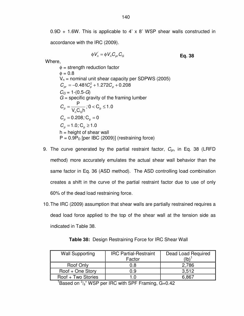
Roof Only 0.8 1.5 1.2 Roof + One Story 0.9 1.33 1.2
Roof + Two Stories 1.0 1.2 1.2 1. These factors are limited to residential construction in accordance with the 2009 IRC and
bracing methods that have a nominal shear strength “capped” at about 700 plf.
Therefore, a PRSW has a 20% advantage to a fully restrained shear wall that
does not include the whole building factor. The committee placed a further limit on the
brace wall requirements. This limit is that the net uplift at the top of the brace wall shall
not exceed 100 plf. If this is exceeded, then an additional connection at the base of the
wall is required.
2.2.2 2009 IRC Requirements
The IRC has several options for providing lateral bracing to a residential
structure. The lateral forces on the structure are resisted by braced wall panels. The
16
braced wall panels can be constructed with either continuous sheathing methods or
intermittent bracing methods. Intermittent braced wall panels can include diagonal let-in
bracing, diagonal sheathing, horizontal siding, or portals. The option which is the focus
of this thesis is intermittent braced wall panel construction, as shown in Figure 2,
utilizing the Wood Structural Panel (WSP) bracing option. The WSP option can be
thought of as a shear wall but is constructed differently than traditional engineered wood
shear walls, i.e. they may not have a special hold down connector.
Figure 2: IRC Braced Wall Panel Location (IRC)
The IRC provides a prescriptive method of lateral bracing for residential
structures. The bracing requirements are dependent upon both wind loads and seismic
loads. For each lateral load condition, the IRC tabulates the total length of braced wall
panels per braced wall line as well as braced wall line spacing. A braced wall line is a
wall selected by the designer to contain braced wall panels. The designer then selects
the braced wall panel type. The braced wall panels must then be located within the
Figure 602.10.1.4(2) Excerpted from the 2009 International Residential Code, Copyright 2009. Washington, D.C.: International Code Council. Reproduced with permission. All rights reserved. www.ICCSAFE.org
17
braced wall lines as specified in the IRC. For WSP, the minimum panel width for the
intermittent brace panel method is 48” and the minimum panel thickness is 3/8”. This
thesis will be limited to wind loading and not seismic loading.
Figure 3: IRC Braced Wall Panel Length
The IRC tabulates the braced wall panels by basic wind speed varying from
85 m.p.h. to 110 m.p.h. A series of adjustment factors are then applied to the tabulated
length of brace wall panels. These factors include: exposure and building height
adjustment; roof to eave height adjustment; number of braced wall line adjustment (to
account for increased shear on braced wall lines from continuous diaphragms, see
discussion below); and an adjustment factor if gypsum or equivalent is not installed on
the interior face of the wall panel. An example of a required length of a braced wall line
is given in Figure 3.
The IRC also specifies all of the connections required for the braced wall panels
as well as the connections of the structure to the wall panels. This includes the
sheathing fastening to the studs, the studs to the plates, the sole plate to the floor or
8'Say L ←=××××= '94.74.19.07.00.19'
Wind Speed = 90 mph → 9’ Braced Panel Length Required Exposure B, 1 Story, 8 ft walls → Multiply x1 Roof Eave-to-Ridge Height <6’ → Multiply by 0.7 and 0.9 No gypsum on interior → Multiply by 1.4 Required Braced Panel Length including all factors:
From IRC Section R602.10.1.2 and Table R602.10.1.2(1)
18
foundation, and the roof or floor to the wall top plate. The sheathing fastening is typical
for a braced wall panel and ordinary sheathing.
The IRC bracing method distributes the lateral loads equally amongst brace wall
panels. This is because it is assumed that the braced wall lines have the minimum
lengths of brace wall panels and therefore are of equal stiffness. Whole building tests
have shown that roof systems behave more like rigid diaphragms than flexible
diaphragms (Crandell and Kochkin 2003). Therefore, the IRC includes an adjustment
factor to increase the length of the braced wall when two or more brace wall lines exist.
This factor is 1.3 for 3 braced wall lines, 1.45 for 4 braced wall lines, and 1.6 for 5 or
more braced wall lines.
Aside from the combined partial restraint and whole building factor of 1.2
discussed earlier, the IRC uses a rational approach. For WSP, the nominal brace wall
capacity used is 700 plf which includes 200 plf capacity for ½” gypsum applied to the
interior face (Crandell and Martin 2009). Using allowable stress design (ASD), a factor
of safety of 2 was applied to the nominal value. This is in accordance with the 2005
Special Design Provisions for and Seismic (AF&PA SDPWS).
2.3 Differences between Prescriptive and Engineered Solutions
The major difference between the prescriptive design of the 2009 IRC and a
rational design using SDPWS is that the IRC applies a combined partial restraint and
whole building factor of 1.2 discussed earlier. An engineered design typically neglects
any applied dead load to the wall and requires a special hold down connector. This is
illustrated in Figure 4.
19
Figure 4: Engineered Shear Wall Restraint Methods
In order to resist the uplift force in a WSP shear wall, one of three methods must
be present for equilibrium. These are a special hold down connector, a dead load force
applied at the tension chord, or some other dead load applied along the wall. It is
common engineering practice to provide a special hold down connector neglecting any
dead loads. This assures that there is a proper load path to resist the overturning of
the wall. If a dead load occurs directly over the tension chord, this could be used to
restrain or partially restrain the wall, but it has a major limitation for an engineered
approach. This limitation is the load combination that requires using only 60% of the
dead load to resist wind overturning forces (ASCE 7). This 40% reduction can have a
huge impact on the uplift resistance. For the last option, special fastening of the wall
sheathing is required. From a mechanics analysis of the wall, the sheathing resists the
V
T C
V
V
P
C
V
HOLD DOWNCONNECTOR
a) Restrained With Hold Downs b) Restrained With Dead Load
20
shear and therefore the sheathing must be resisted from overturning. Therefore, it is
necessary to transmit, for example, a uniform dead load applied to the top of the wall
from the wall studs to the sheathing. This may require closer fastener spacing along the
studs near the end of the wall than would otherwise be specified if a mechanical
restraint was applied directly to the tension chord.
These differences in design approaches make a huge difference when trying to
add a braced wall line or a complete bracing design based on SDPWS to a residential
structure that doesn’t meet the criteria to use the prescriptive method. Although the
whole building factor may be different for a building that meets the prescriptive criteria
than for a building that may have larger wall openings or otherwise doesn’t meet the
prescriptive criteria, there should be some whole building factor that applies to a design
based on SDPWS as well. Also, what effect does the 40% reduction in dead load to
resist overturning per the code imposed load combinations have on the reliability of the
prescriptive system without hold downs?
2.4 Actual Wind Load on a Shear Wall
There are several factors that determine the actual wind load on a shear wall.
The first main factor is on the load side of the design equation. There are several
variables to consider in determining the wind load using ASCE 7. The second main
factor is the load path. A simple analysis may consider flexible diaphragms, while a
more complex analysis may consider a rigid diaphragm.
To determine the wind load on a structure, the location must be known as well as
site conditions. ASCE 7 provides a wind speed map for the United States for the
building designer to determine the nominal 3 second wind gust at a height of 33 feet
21
above the ground for an exposure C terrain category with a 2% probability of
occurrence. ASCE 7 provides two methods to calculate the design wind pressure, the
simplified procedure and the analytical procedure. Either procedure relies upon the
following factors to adjust wind for specific site conditions:
Of the adjustments noted, only the exposure, topographic, and height would vary
from building to building for a residential structure. Of course, the wind speed can vary
as well depending upon the location. However, more than 90 percent of conventional
building stock is located in an Exposure B category based on experimentally controlled
building assessments (Crandell and Kochkin 2003). Additionally, high wind regions
typically require additional bracing and detailing to prevent cladding breaches.
Therefore, the limit of this thesis will be for a nominal wind speed of 90 mph and an
Exposure B category.
ASCE 7 further adds a requirement to design wind pressures, that the minimum
wind pressure shall be 10 psf acting normal to the projected area of the structure in the
direction of the wind, as an additional load case. According to the spreadsheet
calculations available to support the 2009 IRC code change (RB148), the required
10 psf minimum wind load was not used for the prescriptive method in the IRC (FSC).
22
This can make an appreciable difference in the total wind load for this type of structure
with this exposure category.
Residential structures typically don’t have ideally constructed diaphragms
(Crandell and Kochkin 2003) nor are they simple rectangular diaphragms. For more
contemporary homes, it is not uncommon to have a break in the diaphragm such as at a
bridge or two story room. For these reasons, actual wall shear forces may vary
considerably for an actual structure compared to the idealized structures of the IRC
prescriptive design. Therefore, there may be appreciable differences in the actual load
on a braced wall panel when a structure-specific engineering analysis is performed then
the simplified analysis used for the prescriptive method of the IRC.
2.5 Partially and Unrestrained Shear Walls
A great deal of shear wall testing has been performed since as early as 1929
(Crandell and Kochkin 2003). So much testing and studying has occurred since 1983
that John van de Lindt, PhD prepared a paper titled Evolution of Wood Shear Wall
Testing, Modeling, and Reliability Analysis: Bibliography (van de Lindt 2004) This
document tabulates much of the research that was performed, but is not intended to be
inclusive of all work.
The beginning of the acceptance of an unrestrained shear wall in the United
States seems to stem from the perforated shear wall (PSW) method that the American
Forest & Paper Association/American Wood Council (AF&PA/AWC) discovered from
Japan (Crandell 2007). Although the PSW method did require hold downs at each end,
the method allowed for full height openings within the shear wall. Previous to this
23
method, the shear wall was considered a series of shorter shear walls, called a
segmented wall, with each segment requiring hold downs.
The PSW method still didn’t correlate with conventional construction practices of
not providing hold downs. Thus research began to develop a design method to
construct shear walls without hold downs (Crandell 2007). This included using corners
as restraint (Dolan and Heine 1997) and PRSW (Ni and Karacabeyli 2000). Walls with
IRC prescribed anchorage compared to full restraint (mechanical hold down) and partial
restraint by an applied load was conducted to compare the difference between
monotonic and cyclic loading (Seaders 2004). The PRSW method (Ni and Karacabeyli
2000) is of interest since it presents both a mechanics-based method and an empirical
method to determine the capacity of the wall under partial restraint. Also of interest is
the IRC prescribed anchorage monotonic and cyclic comparison study.
Many factors can affect the shear capacity of a PRSW (Crandell and Martin
2009). These conditions include:
• Length of wall extending beyond either end of the bracing element • Wall components or opening conditions adjacent to a bracing element • Support conditions (framing assembly stiffness and dead load above the
bracing element) • Strength of bracing method relative to strength of conventional framing
and connections providing restraint to a given brace panel at its boundaries.
• Contribution of non-structural components and non-compliant bracing elements in a whole house test.
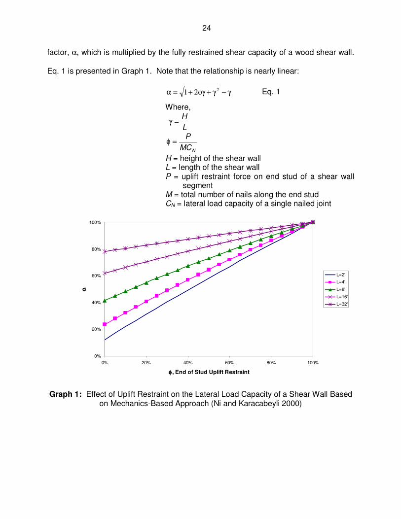
The mechanics-based method derived in Ni and Karacabeyli (2000) assumes
that some of the boundary fasteners in the sole plate are used only for the uplift
resistance while the remaining fasteners resist the shear. The result is the reduction
24
factor, α, which is multiplied by the fully restrained shear capacity of a wood shear wall.
Eq. 1 is presented in Graph 1. Note that the relationship is nearly linear:
γ−γ+φγ+=α 221
Eq. 1
Where,
L
H=γ
NMC
P=φ
H = height of the shear wall L = length of the shear wall P = uplift restraint force on end stud of a shear wall
segment M = total number of nails along the end stud CN = lateral load capacity of a single nailed joint
0%
20%
40%
60%
80%
100%
0% 20% 40% 60% 80% 100%
φφφφ , End of Stud Uplift Restraint
αα αα
L=2'
L=4'
L=8'
L=16'
L=32'
Graph 1: Effect of Uplift Restraint on the Lateral Load Capacity of a Shear Wall Based on Mechanics-Based Approach (Ni and Karacabeyli 2000)
25
Using the results of both monotonic and cyclic testing, the ratio of the lateral load
capacity of a wall with no restraint to a wall with full restraint, α, the following empirical
relationship was determined (Ni and Karacabeyli 2000).
3)1(1
1
φ−γ+=α
Eq. 2
This equation is presented graphically in Graph 2.
Although Graph 2 seems to indicate that there is no uplift restraint, i.e. φ=0, the
test method used to develop Eq. 2 used ½” diameter anchor bolts at 16” o.c. with the
first bolt 8” from the end of the wall, providing some uplift resistance.
0%
20%
40%
60%
80%
100%
0% 20% 40% 60% 80% 100%
φφφφ , End of Stud Uplift Restraint
αα αα
L=2'
L=4'
L=8'
L=16'
L=32'
Graph 2: Effect of Uplift Restraint on the Lateral Load Capacity of a Shear Wall Based on Empirical Approach (Ni and Karacabeyli 2000)
The SDPWS also provides a method for designing PSW, but still requires hold
downs at the very ends of the wall. This method allows for unrestrained segments
within the length of the wall.
26
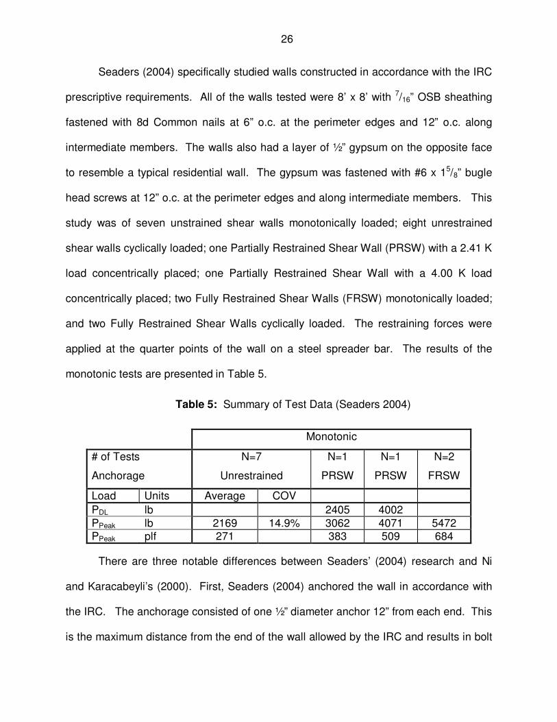
Seaders (2004) specifically studied walls constructed in accordance with the IRC
prescriptive requirements. All of the walls tested were 8’ x 8’ with 7/16” OSB sheathing
fastened with 8d Common nails at 6” o.c. at the perimeter edges and 12” o.c. along
intermediate members. The walls also had a layer of ½” gypsum on the opposite face
to resemble a typical residential wall. The gypsum was fastened with #6 x 15/8” bugle
head screws at 12” o.c. at the perimeter edges and along intermediate members. This
study was of seven unstrained shear walls monotonically loaded; eight unrestrained
shear walls cyclically loaded; one Partially Restrained Shear Wall (PRSW) with a 2.41 K
load concentrically placed; one Partially Restrained Shear Wall with a 4.00 K load
concentrically placed; two Fully Restrained Shear Walls (FRSW) monotonically loaded;
and two Fully Restrained Shear Walls cyclically loaded. The restraining forces were
applied at the quarter points of the wall on a steel spreader bar. The results of the
There are three notable differences between Seaders’ (2004) research and Ni
and Karacabeyli’s (2000). First, Seaders (2004) anchored the wall in accordance with
the IRC. The anchorage consisted of one ½” diameter anchor 12” from each end. This
is the maximum distance from the end of the wall allowed by the IRC and results in bolt
27
spacing of 6’, the maximum spacing allowed by the IRC. Second, Seaders (2004) used
gypsum on the opposite face of the wall than the WSP. The intent was to apply the
dead load of the gypsum rather than add additional stiffness from the gypsum. It is
important to note that the fastener spacing in the gypsum was 12” o.c. throughout
compared with 7” o.c. specified in the IRC. Third, Seaders (2004) compared the
variability of monotonic testing with the variability of cyclic testing while Ni and
Karacabeyli (2000) proposed a method of determining the capacity of an unrestrained
wall.
It is very important to point out that both Seaders (2004) and Ni and
Karacabeyli’s (2000) work considered the full restraint capacity as the capacity of the
shear wall with a mechanical hold down at the base of the wall. Therefore, Ni and
Karacabeyli’s (2000) partial restraint factor, Eq. 2, is derived from the capacity of the
wall when a mechanical hold down is used at the base of the wall.
2.6 Special Design Provisions for Wind and Seismic (2005)
The SDPWS (2005) provides design methodologies for wood diaphragms and
shear walls and contains nominal ultimate unit shear capacities for shear walls
constructed with WSPs. These capacities are tabulated for various thickness sheathing
and fastener spacing for both wind and seismic. The values in these tables are 2.8
times the values given in APA Research Report 154 (2004), the source of the
capacities. APA Research Report 154 (2004) will be discussed later. SDPWS (2005) is
also the source of the semi-rational design values for the 2009 IRC.
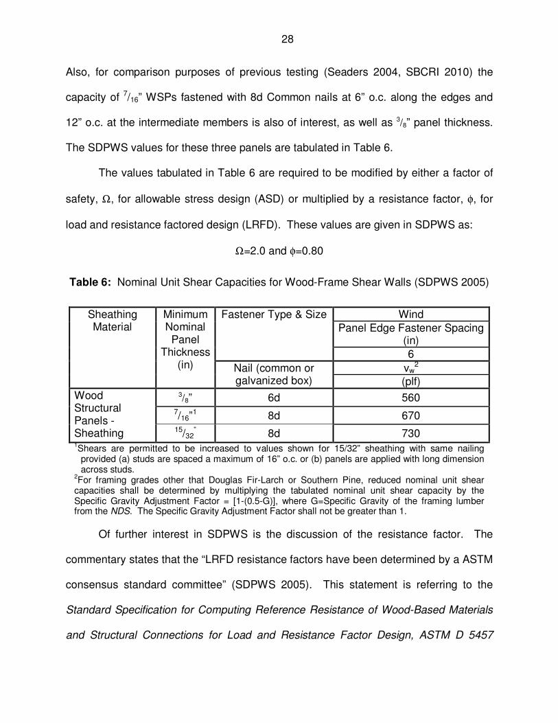
Of interest to this research is the capacity of the 15/32” WSP fastened with 8d
Common nails at 6” o.c. along the edges and 12” o.c. at the intermediate members.
28
Also, for comparison purposes of previous testing (Seaders 2004, SBCRI 2010) the
capacity of 7/16” WSPs fastened with 8d Common nails at 6” o.c. along the edges and
12” o.c. at the intermediate members is also of interest, as well as 3/8” panel thickness.
The SDPWS values for these three panels are tabulated in Table 6.
The values tabulated in Table 6 are required to be modified by either a factor of
safety, Ω, for allowable stress design (ASD) or multiplied by a resistance factor, φ, for
load and resistance factored design (LRFD). These values are given in SDPWS as:
Ω=2.0 and φ=0.80
Table 6: Nominal Unit Shear Capacities for Wood-Frame Shear Walls (SDPWS 2005)
Wind
Panel Edge Fastener Spacing (in)
Fastener Type & Size
6
vw2
Sheathing Material
Minimum Nominal
Panel Thickness
(in) Nail (common or galvanized box) (plf)
3/8” 6d 560 7/16”
1 8d 670
Wood Structural Panels -Sheathing 15/32
” 8d 730 1Shears are permitted to be increased to values shown for 15/32” sheathing with same nailing provided (a) studs are spaced a maximum of 16” o.c. or (b) panels are applied with long dimension across studs.
2For framing grades other that Douglas Fir-Larch or Southern Pine, reduced nominal unit shear
capacities shall be determined by multiplying the tabulated nominal unit shear capacity by the Specific Gravity Adjustment Factor = [1-(0.5-G)], where G=Specific Gravity of the framing lumber from the NDS. The Specific Gravity Adjustment Factor shall not be greater than 1.
Of further interest in SDPWS is the discussion of the resistance factor. The
commentary states that the “LRFD resistance factors have been determined by a ASTM
consensus standard committee” (SDPWS 2005). This statement is referring to the
Standard Specification for Computing Reference Resistance of Wood-Based Materials
and Structural Connections for Load and Resistance Factor Design, ASTM D 5457
29
(ASTM D 5457). The resistance factors were reportedly “derived to achieve a target
reliability index, β, of 2.4 for a reference design condition” (SDPWS 2005).
SDPWS also has a method for determining the capacity of intermittent bracing
known as the Perforated Shear Wall (PSW) as mentioned earlier. The 2009 IRC used
the PSW method to approximate the partial restraint factor. The PSW method in the
SDPWS differs from Ni and Karacabeyli’s (2000) method to determine the capacity of a
PRSW.
SDPWS uses a shear capacity adjustment factor, Co, to modify the nominal
shear capacities of the full height sheathed wall segment which is a function of the wall
openings and the length of the wall. For intermittent shear walls, Co is determined
assuming that all openings are full height. It is tabulated in SDPWS as a function of the
percent of full-height sheathing. The tabulated values of Co are calculated as shown in
Eq. 3.
height wall
openings of area total
ratio area sheathing
1
1
23
sheathing height-full of widththe of sumL
wallshear of length total
Sheathing Height-Full of %FH %
where,
FH %
F
i
0
=
=
=
+
=
−=
=
=
=
=
∑
∑
h
A
r
LhA
r
r
rF
L
C
o
i
o
Eq. 3
30
The IRC originally used a modified version of Eq. 3 to estimate the partial
restraint factors indicated in Table 4. The modified version used F=r/(2-r) deemed to be
more accurate and less conservative (Crandell 2007). The lowest value of Co tabulated
in SDPWS is for 10% full-height sheathing and is equal to 0.36, which for 4’ shear walls
equates to a 5% restraining force using Ni and Karacabeyli’s (2000) method. For Co to
equal 0.8 as used in the IRC, 88% of the brace wall line would have to be sheathed at
full height.
The PSW requires restraints at the very ends of the walls, as does a fully
restrained wall. These restraints can be mechanical hold downs or dead load.
Additionally, the sole plate of each full height segment must be anchored to the
foundation for a uniform uplift force equal to the unit shear (SDPWS). This is not a
requirement of the 2009 IRC.
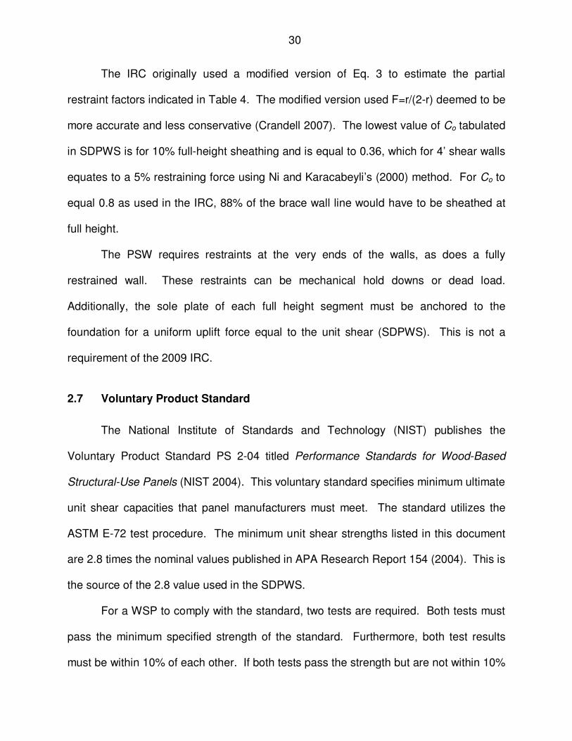
2.7 Voluntary Product Standard
The National Institute of Standards and Technology (NIST) publishes the
Voluntary Product Standard PS 2-04 titled Performance Standards for Wood-Based
Structural-Use Panels (NIST 2004). This voluntary standard specifies minimum ultimate
unit shear capacities that panel manufacturers must meet. The standard utilizes the
ASTM E-72 test procedure. The minimum unit shear strengths listed in this document
are 2.8 times the nominal values published in APA Research Report 154 (2004). This is
the source of the 2.8 value used in the SDPWS.
For a WSP to comply with the standard, two tests are required. Both tests must
pass the minimum specified strength of the standard. Furthermore, both test results
must be within 10% of each other. If both tests pass the strength but are not within 10%
31
of each other, then a third test may be performed. The lowest two of the three tests
must then exceed the strength requirement and must be within 10% of each other. The
standard does not have values for all nail spacings used in the SDPWS.
2.8 APA Research Report 154
APA-The Engineered Wood Association publishes APA Research Report 154
titled Wood Structural Panel Shear Walls (APA 2004). The source for the SDPWS
tabulated nominal ultimate unit shear values is from the base values in the APA
Research Report 154 (2004). The APA Research Report 154 (2004) values match the
tabulated nominal ultimate unit seismic shear values in the SDPWS. The wind values
tabulated in the SDPWS are 40% greater than APA Research Report 154 (2004)
values.
The nominal unit shear values tabulated in APA Research Report 154 (2004) are
historic values from the 1958 to 1964 Uniform Building Codes. APA Research Report
154 (2004) provides a comparison of the nominal unit shear values to previous tests
and is shown here in Table 7. The target design shear is the nominal unit shear values
tabulated in APA Research Report 154 (2004) or 1/2.8 the tabulated nominal ultimate
unit shear values for wind tabulated in SDPWS and the nominal minimum ultimate unit
shear values tabulated in PS-2 (2004).
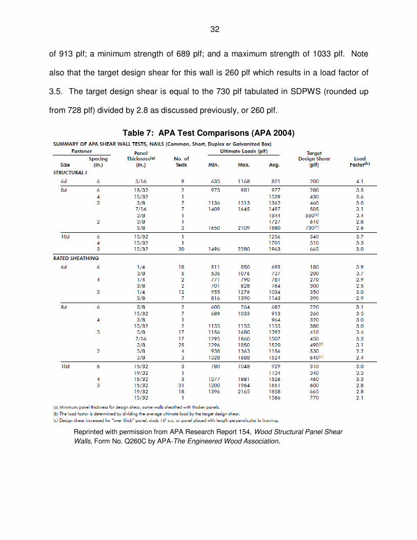
The comparison in Table 7, noted as the load factor, is between the average test
results and the target design shear and ranges from 2.1 to 4.1. Table 7 also indicates
the number of tests used for the comparison as well as the minimum, maximum, and
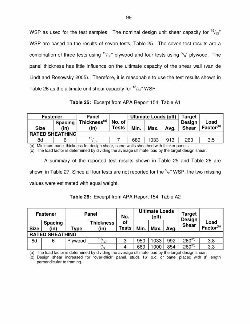
average ultimate load. Of interest is the 15/32” rated sheathing with 8d nails spaced at
6” o.c. The table provides the results of seven tests with an average ultimate strength
32
of 913 plf; a minimum strength of 689 plf; and a maximum strength of 1033 plf. Note
also that the target design shear for this wall is 260 plf which results in a load factor of
3.5. The target design shear is equal to the 730 plf tabulated in SDPWS (rounded up
from 728 plf) divided by 2.8 as discussed previously, or 260 plf.
Table 7: APA Test Comparisons (APA 2004)
Reprinted with permission from APA Research Report 154, Wood Structural Panel Shear
Walls, Form No. Q260C by APA-The Engineered Wood Association.
33
2.9 Shear Wall Strength and Computer Modeling
Shear wall strength can be either calculated (mechanistic) or determined from
testing (hysteresis). A mechanistic model is provided in APA Research Report 154
(2004) for determining the capacity of a fully restrained shear wall. This model is based
on the nail capacities in the NDS (2005). The mechanistic model simply resolves the
applied shear along the sole plate and the uplift force into the tension stud through the
fasteners in a unidirectional shear in the direction of the sole plate and tension chord
respectively. Cyclic testing is used to determine the nonlinear load-deformation
response of a shear wall. From this testing the hysteresis curves are produced. The
backbone curve, also referred to as the envelope curve, is formed from the peaks of the
hysteresis curves. The backbone curve, shown in Figure 5, closely approximates the
nonlinear load deformation curve produced from a monotonic test (van de Lindt 2003).
Figure 5: Hysteresis Curve Example
0.0
0.0
Backbone Curve
34
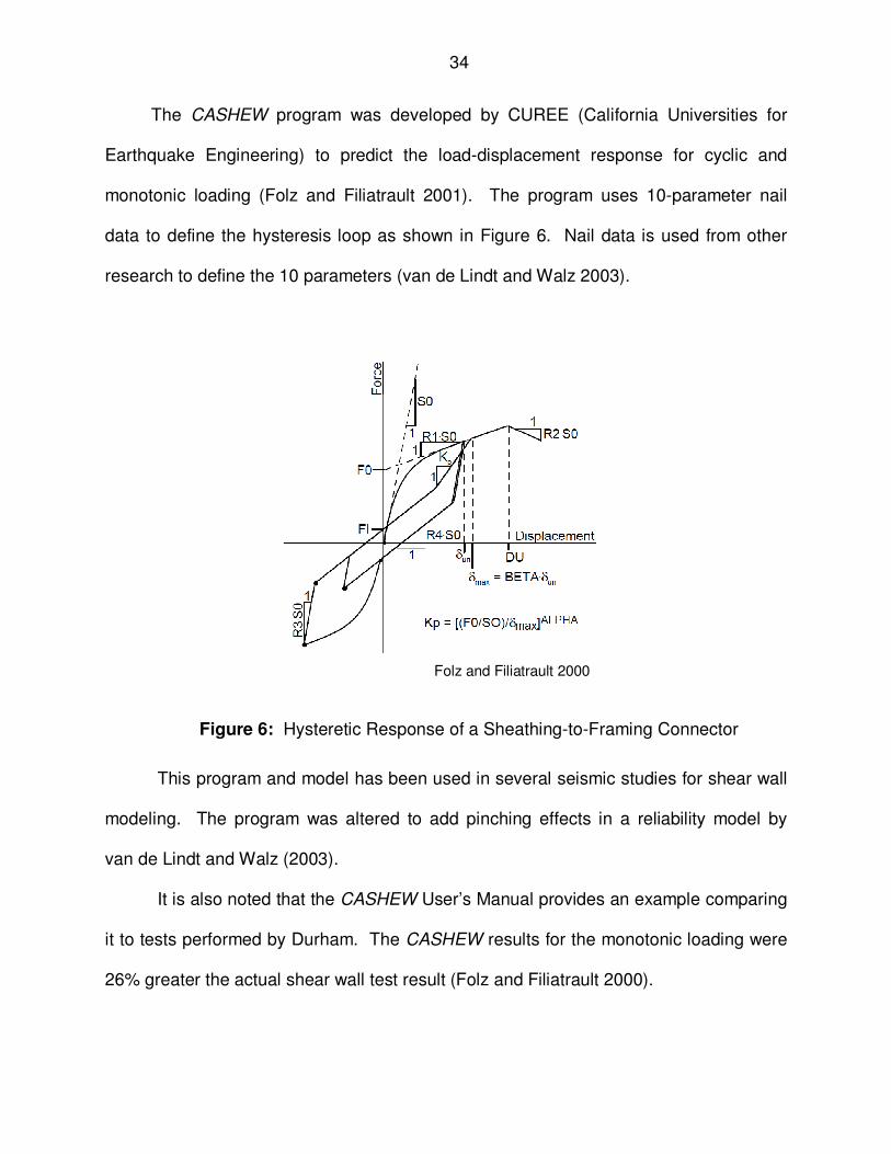
The CASHEW program was developed by CUREE (California Universities for
Earthquake Engineering) to predict the load-displacement response for cyclic and
monotonic loading (Folz and Filiatrault 2001). The program uses 10-parameter nail
data to define the hysteresis loop as shown in Figure 6. Nail data is used from other
research to define the 10 parameters (van de Lindt and Walz 2003).
Figure 6: Hysteretic Response of a Sheathing-to-Framing Connector
This program and model has been used in several seismic studies for shear wall
modeling. The program was altered to add pinching effects in a reliability model by
van de Lindt and Walz (2003).
It is also noted that the CASHEW User’s Manual provides an example comparing
it to tests performed by Durham. The CASHEW results for the monotonic loading were
26% greater the actual shear wall test result (Folz and Filiatrault 2000).
Folz and Filiatrault 2000
35
2.9.1 Finite Element Modeling
Several studies have been done using finite element
modeling (FEM) of wood shear walls. These studies have
evolved over the years and can be rather simplistic models
or more complex models that account for every connection
in the wall. The programs used for the finite element
include commercial programs such as ABAQUS and ANSYS. Others have developed
programs as well, such as SHWALL and CASHEW.
This work is best summarized by Cassidy (2002) and Judd (2005). The most
common models include beam elements for framing members, four and eight node
plane stress elements for sheathing, and two orthogonal nonlinear springs (or spring
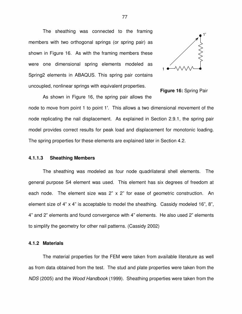
pair), Figure 7, to model the connections from the sheathing to the framing members
(e.g. Dolan and Foschi 1991; Folz and Filiatrault 2001; Cassidy 2002; Judd 2005).
Of the referenced examples, Judd, using ABAQUS, created an oriented spring
pair as a user element. Judd recognized that for nonlinear springs, the bilinear spring
isn’t equivalent to a single one dimensional spring. For monotonic loading, the peak
load and displacement can be accurately calculated with a bilinear spring element.
However, the total energy absorbed by the system is not accurate with the bilinear
spring, since the load deformation curve does not completely represent the behavior of
the actual wall (Cassidy 2002). The increased resultant stiffness overestimates the total
energy absorbed.
The most common method of modeling the framing connections is with pinned
joints (e.g. Judd 2005, CASHEW). The results of these models reasonably match the
1
1’
Figure 7: Spring Pair
36
test walls that they were developed for, but this type of model doesn’t accurately
capture the actual behavior of the wall. Cassidy (2002) used another spring pair to
model the behavior of the stud to plate connection. The spring pair had differing
stiffness for the load direction.
Using a typical stud-to-plate connection of two 16d Common nails, Cassidy
(2002) used a lateral stiffness of 12,000 lb/in which corresponds to results published by
Dolan et. al. (1995). Cassidy (2002) found that this parameter had “very little effect on
the overall load-displacement response of the wall.” Cassidy (2002) used a nonlinear
vertical stiffness. For compression, a vertical stiffness of 41,000 lb/in was used which
corresponds to his reported test results for the crushing of the wood sole plate. Cassidy
then used a tension stiffness of 100 lb/in. This was an assumption by Cassidy. The
vertical tension stiffness of course relates to nails installed in the end grain of the stud
loaded in withdrawal. According to the NDS Commentary (AF&PA 2005), there can be
up to a 50% reduction in nail withdrawal strength into end grain, and coupling this with
seasoning, the values are deemed too unreliable and are prohibited. However, there is
definitely some resistance and stiffness in this connection; although not reported to the
author’s knowledge.
2.9.2 Sheathing Nail Modeling
Sheathing nail modeling is considered in two ways. The first is considering the
yield limit equations from the NDS (AF&PA 2005). The second is considering the load
deformation relationship of the fasteners. The latter is of interest for finite element
modeling while the former is helpful in the understanding of allowable nail capacities
published in the NDS.
37
2.9.2.1 NDS Yield Limit Equations
The yield limit equations in the NDS (AF&PA 2005) provide a method to calculate
nail connection strength based on limit states or modes of failure. The yield limit
equations are a mechanics based method. Technical Report 12 (AF&PA 1999)
expands on the yield limit equations used in the NDS (AF&PA 2005). The modes of
failure of a dowel-type connection are “uniform bearing under the fastener, rotation of
the fastener in the joint without bending, and development of one or more plastic hinges
in the fastener.” (AF&PA 1991). Technical Report 12 (AF&PA 1999) provides the basis
for calculating the ultimate nail capacity for each mode of failure by considering the
specific gravity of the material, the thickness of each member, any gap that may exist
between the members, and the yield strength of the fastener. This is not the failure
load, but is rather the ultimate load. The failure load occurs after the ultimate load is
reached.
For single shear, there are four modes of failure to consider, Figure 8. These
modes are briefly described and explained here. They are based on no gap between
the members. Additionally, Technical Report 12 (AF&PA 1999) provides methods for
calculating the failure load at the proportional limit, the 5% offset limit, and the ultimate
limit. Only the ultimate limit is presented here.
38
Reprinted with permission from Technical Report 12, General Dowel Equations for
Calculating Lateral Connections by the American Wood Council, Leesburg, VA
Figure 8: Connection Yield Modes
39
2.9.2.1.1 Mode Im and Is
The limit state for failure mode I is either wood bearing in the main member (Im)
or wood bearing in the side member (Is) with no rotation or yielding of the fastener.
Mode I strength is:
Im mm lqP = Eq. 4
Is ss lqP = Eq. 5
2.9.2.1.2 Mode II
The limit state for failure mode II is side and main member wood bearing with
rigid rotation of the fastener, but no yielding of the fastener. Mode II strength is:
II A
ACBBP
2
42 −+−= Eq. 6
where,
ms qqA
4
1
4
1+=
22ms ll
B += 44
22
mmss lqlqC −−=
2.9.2.1.3 Mode IIIm and IIIs
The limit state for failure mode III is either main member bearing and yielding of
the fastener in the side member (IIIm) or side member bearing and yielding of the
fastener in the main member (IIIs). Mode IIIm and IIIs strength is defined by Eq. 6 where,
IIIm ms qq
A4
1
2
1+=
2mlB =
4
2
mms
lqMC −−=
IIIs ms qq
A2
1
4
1+=
2slB =
mss M
lqC −−=
4
2
40
2.9.2.1.4 Mode IV
The limit state for failure mode IV is yielding of the fastener in both the side and
the main member. Mode IV strength is defined by Eq. 6 where,
IV ms qq
A2
1
2
1+= 0=B ms MMC −−=
For all modes, the following definitions are used,
P = nominal lateral connection value, lb ls = side member dowel bearing length, in lm = main member dowel bearing length, in qs = side member dowel bearing resistance = FesD, lb/in qm = side member dowel bearing resistance = FemD, lb/in Fes = side member dowel bearing strength, psi Fem = main member dowel bearing strength, psi D = dowel shank diameter, in Fb = dowel bending strength, psi Ds = dowel diameter at max. stress in side member, in Dm = dowel diameter at max. stress in main member, in Ms = side member dowel moment resistance = Fb(Ds
3/6) Mm = main member dowel moment resistance = Fb(Dm
3/6) Fe = 0.8 x 11735G1.07/D0.17, psi (parallel to grain) G = specific gravity Fb = Fb, ult, psi
All of the limit states must be checked to determine the failure load of the
fastener. The failure load is then the least of modes Im, Is, II, IIIm, IIIs, and IV.
2.9.2.2 Load Deformation of Nails
Several methods for modeling the load deformation have been developed over
the years. According to Judd (2005), these range from power curve (Mack 1977; APA),
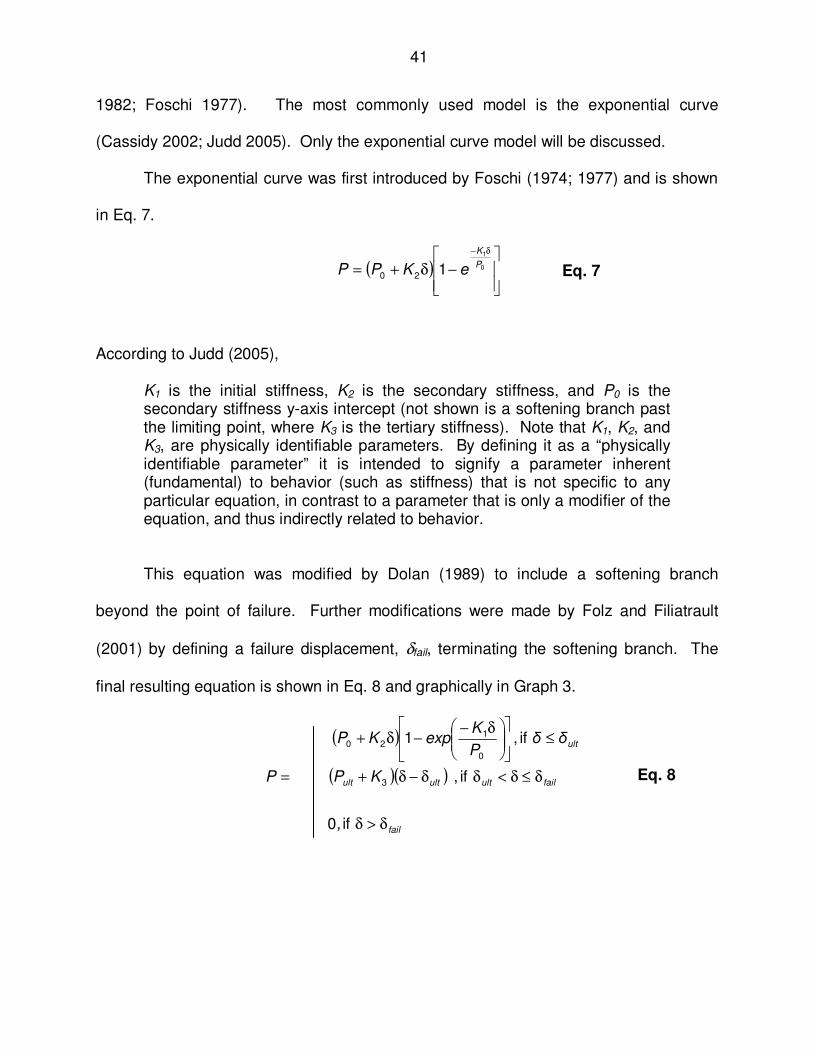
1982; Foschi 1977). The most commonly used model is the exponential curve
(Cassidy 2002; Judd 2005). Only the exponential curve model will be discussed.
The exponential curve was first introduced by Foschi (1974; 1977) and is shown
in Eq. 7.
( )
−δ+=
δ−
0
1
120P
K
eKPP Eq. 7
According to Judd (2005),
K1 is the initial stiffness, K2 is the secondary stiffness, and P0 is the secondary stiffness y-axis intercept (not shown is a softening branch past the limiting point, where K3 is the tertiary stiffness). Note that K1, K2, and K3, are physically identifiable parameters. By defining it as a “physically identifiable parameter” it is intended to signify a parameter inherent (fundamental) to behavior (such as stiffness) that is not specific to any particular equation, in contrast to a parameter that is only a modifier of the equation, and thus indirectly related to behavior.
This equation was modified by Dolan (1989) to include a softening branch
beyond the point of failure. Further modifications were made by Folz and Filiatrault
(2001) by defining a failure displacement, δfail, terminating the softening branch. The
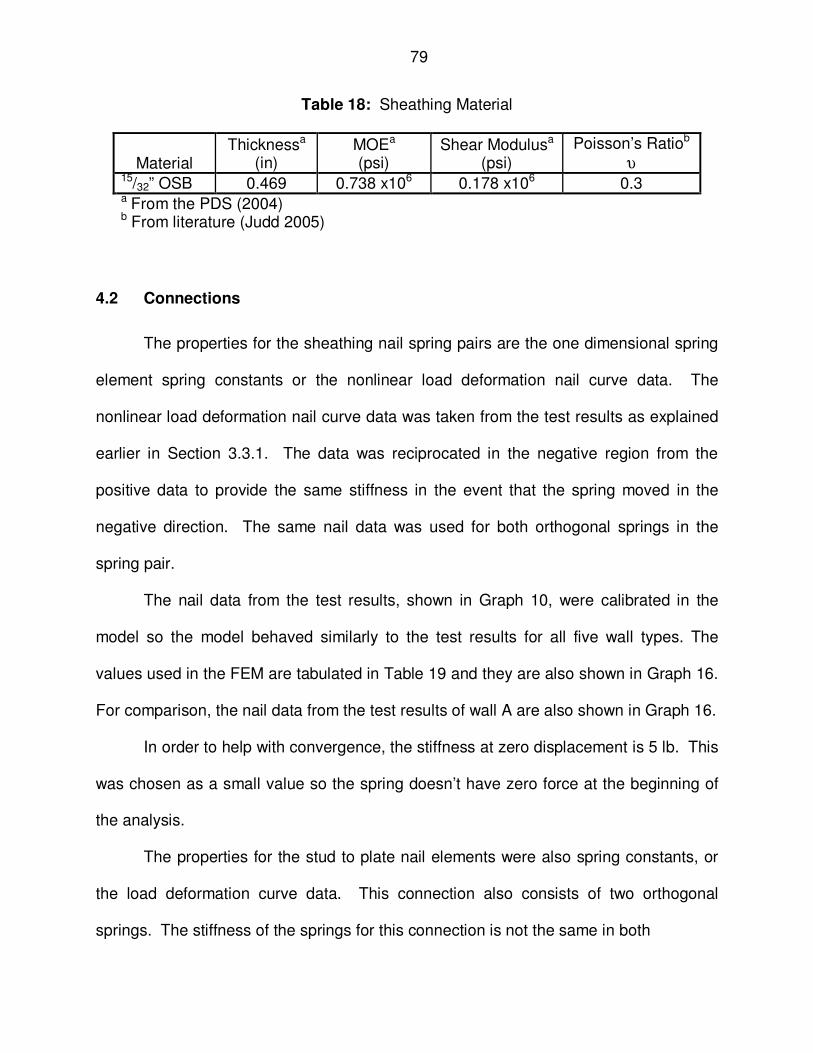
final resulting equation is shown in Eq. 8 and graphically in Graph 3.
( )
( )( )
fail
failultultult
ult
,
KPP
δδP
KexpKP
δ>δ
δ≤δ<δδ−δ+=
≤
δ−−δ+
if 0
if ,
if , 1
3
0
120
Eq. 8
42
Graph 3: Nail Deformation Model
Displacement, in
Lo
ad
, lb
δδ ult
P
P o
K 1
1
K 2
1
K 3
1
δ fail
2.10 Reliability Studies
Reliability studies have been conducted of wood shear walls for both seismic
(van de Lindt 2004) and wind loads (van de Lindt and Rosowsky 2005). Of interest to
this research is the wind load reliability.
The reliability analysis by (van de Lindt and Rosowsky 2005) used shear wall
construction methods specified in the “Standard for Load and Resistance Factor Design
(LRFD) for Engineered Wood Construction” AF&PA/ASCE 16-95 and used a static-
pushover analysis using the computer program CASHEW (Folz and Filiatrault 2001) to
determine the monotonic load-deflection behavior (van de Lindt and Rosowsky 2005).
The reliability index, β, was found to range from 3.0 to 3.5 with a mean of 3.17 and a
COV = 0.05 (van de Lindt 2005).
43
Wind velocity is modeled as a Gumbel distribution or Type I (Ellingwood et al,
1980). This distribution is an extreme value distribution which is asymptotic with a
Cumulative Distribution Function (CDF) given as the double exponential function shown
in Eq. 9 (Ang and Tang 1975):
( ) ( )( )[ ] ∞<<∞−−α−−= xuxexpexpxFX Eq. 9
Although the wind velocity has a Type I distribution, this doesn’t necessarily mean that
the wind load has a Type I distribution since the wind load is a function of the velocity
squared. However, this relationship was studied considering the other random
variables (pressure coefficients, exposure factor and gust factor) that influence the wind
load and it was determined that the probability distribution of wind load is also a Type I
distribution (Ellingwood et al, 1980)
Van de Lindt used the model suggested by Ellingwood (1999). For this model,
the 50-year maximum wind load is modeled as a Type I random variable, shown in
Graph 4. The bias factor (mean-to-nominal value), including directionality effects, is
given by:
80.W
W
N
= Eq. 10
where, W = mean wind load WN = nominal (code-specified) wind load
The coefficient of variation is 0.35 (van de Lindt and Rosowsky 2005). Van de Lindt’s
model considered the capacity of the shear wall given in SDPWS multiplied by the
strength reduction factor, φ, (the load with a Type I distribution) as the random variable.
This was the only random variable used, since the resistance, computed as the ultimate
44
wall strength from CASHEW, was assumed to be deterministic as shown as the vertical
line in Graph 5.
Graph 4: Probability Density Function of Shear Wall Load
Van de Lindt used the limit state in its simplest form to calculate the second-
moment reliability index, β. This limit state is shown here as:
g(x) = R-S Eq. 11
where g(x) is the limit state function, R is the structural resistance, and S is the load
effect. R could be a random variable and S could be a random variable, or they could
be a function of several random variables. As noted earlier, van de Lindt chose to only
use S as a random variable and R as a constant (van de Lindt and Rosowsky 2005).
0 2 4 6 8 10 120
0.1
0.2
0.3
0.4
0.5
0
F x( )
45
For the limit state shown above, failure occurs when g(x) < 0. As shown in the shaded
portion of Graph 5, probability of failure, pf, is the probability that g(x) < 0.
Graph 5: Failure Region of PDF of Shear Wall Load
The reliability index, β, is the inverse of the standard normal distribution function
and is determined by:
( )fp−Φ=β − 11 Eq. 12
β, shown graphically on the standard normal distribution in Graph 6 is a scale of the
standard deviation, σ, to the probability of failure. This allows a measure of structural
safety for any limit state, material, or load.
Probability of Failure, pf g(x)
46
Graph 6: Reliability Index, β, on the Standard Normal Distribution
2.11 IRC Brace wall Testing - SBC Research Institute
The SBC Research Institute tested a 12’ x 30’ structure, Figure 9 and
Figure 10, with IRC prescriptive intermittent walls in early 2010. The test results are
currently available in the SBCRI Tech Note titled 2009 International Residential Code
The inaccuracy of the partial restraint factor, α, is most likely due to the anchor
bolt locations. Recall that the IRC wall is anchored with ½” diameter anchor bolts a
maximum of 12” from the end and 6’ o.c. while Ni and Karacabeyli’s wall tests utilized
½” diameter anchor bolts at 16” o.c. and 8” from the ends. Therefore, some
modification of Eq. 2 is necessary for IRC anchored walls.
The capacity of an unrestrained 3/8” WSP shear wall constructed and anchored
according to the IRC is unknown at this time. If there is a correlation between the 7/16”
and the 3/8” WSP unrestrained, then the unrestrained value of the 3/8” WSP would be
40% of the SDPWS value or one half of the assumed 80% value that the IRC uses.
Therefore, for a lightly loaded wall, the reliability would be much less for the IRC brace
wall than the SDPWS fully restrained wall.
51
CHAPTER 3
TESTING OF SHEAR WALLS
This chapter summarizes the test procedure, test results and numerical data from
the testing of 25 wood shear walls. The 25 shear walls were divided into five groups of
five walls each. The restraint of the shear walls was set differently for all five sets to
understand the effect of partial restraint and full restraint on the shear wall unit shear
capacity.
3.1 Current ASTM Test Procedures
Two ASTM standards exist for shear wall testing. The first is the “Standard Test
Methods of Conducting Strength Tests of Panels for Building Construction” (ASTM
E72-10). The second is the “Standard Practice for Static Load Test for Shear
Resistance of Framed Walls for Buildings” (ASTM E564-00).
The purpose of ASTM E72 is to evaluate different types of sheathing on a
standard wood frame. Since the standard wood frame is the same for all sheathing
materials, the relative difference in performance of the sheathing materials is the test
objective (ASTM E72). Three tests are required by this standard. ASTM E72 employs
an 8’ x 8’ panel (two sheets of WSPs). The frame is constructed with 2x4 studs spaced
at 16” on center with a single 2x4 sole plate and a double 2x4 top plate. Spaced corner
posts are used at each end with fastening to the outside post only. All framing material
is No. 1 Douglas Fir or Southern Pine. Fastening of the WSPs shall follow the
manufacturer’s recommendations. The standard emphasizes the importance of placing
the fasteners exactly in the required location maintaining the correct edge distance and
52
angle (typically perpendicular to the WSP). Figure 11 shows the frame required by
ASTM E72.
Reprinted, with permission, from ASTM E72-10 “Standard Test Methods of Conducting Strength Tests of Panels for Building Construction”, copyright ASTM International, 100 Barr Harbor Drive, West Conshohocken, PA 49428.
Figure 11: Standard Wood Frame (ASTM E72)
ASTM E72 also specifies the loading point, the load rate, a hold down device,
and the points of measurement. The load point is at the end of a timber member bolted
to the double top plate. The hold down device consists of two steel rods extending
53
through a bearing plate with rollers above the corner post at the end where the load is
applied. The rods are installed such that one is located on each side of the frame. The
load rate specifies application of a uniform rate of motion to three steps: 790, 1570, and
2360 lb. The load shall be applied at the same rate for all three steps, but the first step
must be loaded in no more than two minutes. Upon reaching the first load step,
measurements are made at each measurement point and then the wall is unloaded.
Measurements are again made after unloading to determine any permanent
deformation. This process is repeated for the next two load steps. Three points of
measurement are required for this test. They are all horizontal measurements. One
point is located at the end of the double top plate and the remaining two are located at
each end of the sole plate. The displacement measurements must be recorded to the
nearest 0.01”
The purpose of ASTM E564 is to evaluate the shear capacity of any type of light
framed wall supported on a rigid foundation and to determine the shear stiffness and
strength of the wall (ASTM E564). The standard does not dictate a particular hold down
device, but rather specifies the use of the same anchorage and applied axial loads
expected in the service condition. Similarly, the framing members and fastening shall
be the same size, grade and construction as anticipated in actual use.
ASTM E564 also specifies loading requirements. Although similar to ASTM
E72, there are some slight differences between the standards. ASTM E564 requires an
initial load equal to 10% of the anticipated ultimate load to be applied for five minutes to
seat all connections. The initial load is removed and after five minutes the initial
readings of displacement are recorded. The next sequence of loading is then applied in
54
intervals, or load steps, of 1/3, 2/3, and finally, the ultimate load. All of the load steps
are applied at the same rate which is equal to reaching the anticipated ultimate load in
no less than five minutes. At each of these intervals the load step is applied up to the
specified load and held for one minute. The displacements are then recorded, and then
the specimen is unloaded. After five minutes of unloading, the displacements are again
recorded. The process is then repeated until the last load step and ultimate failure is
reached. Ultimate failure may be a displacement limit rather than a load limit.
ASTM E564 provides a method for reporting both the global shear stiffness of the
wall and the internal shear stiffness of the wall as well as the ultimate strength. The
internal shear stiffness of the wall does not include uplift, or rotation, of the entire wall,
but rather only the distortion of the wall itself. The ultimate strength is reported as an
ultimate unit shear strength which is simply the ultimate load divided by the wall width.
ASTM E564 requires testing a minimum of two wall assemblies. If after testing
two assemblies either the shear stiffness or the ultimate strength are not within 15% of
each other, then a third test is required. The strength and stiffness values reported are
then the average of the two weakest specimen values.
3.2 Wall Testing
The following summarizes the test procedure and results of the 25 wood shear
walls used for the reliability analysis. The shear wall testing was conducted at the
Structural Building Components Research institute in Madison, WI in March 2011. The
tests were performed in accordance with ASTM E564. Details of the testing are
presented in Appendix A.
55
3.2.1 Test Facility
The SBCRI test facility has an ACLASS accreditation, Appendix B. ACLASS is
one of two brands of the ANSI-ASQ National Accreditation Board. The accreditation is
for testing full scale construction assemblies and is accredited to ISO/IEC 14025:2005.
Of particular interest, the accreditation specifically encompasses ASTM E564 and
ASTM E72 testing.
The SBCRI test facility is capable of testing both single components and entire
structures up to 30’ wide x 32’ tall x 90’ long. Completely adjustable frames allow for a
large variation of test configurations.
3.2.2 Wall Construction
3.2.2.1 Wall Matrix
The 25 shear walls were constructed identically, except for the anchorage, and
tested identically. The shear walls were grouped in five groups of five walls each for the
testing. See Table 11 for a summary of walls tested. Illustrations of the test setups are
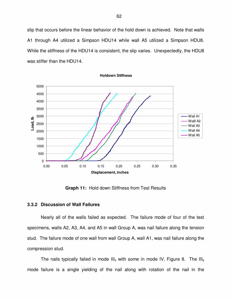
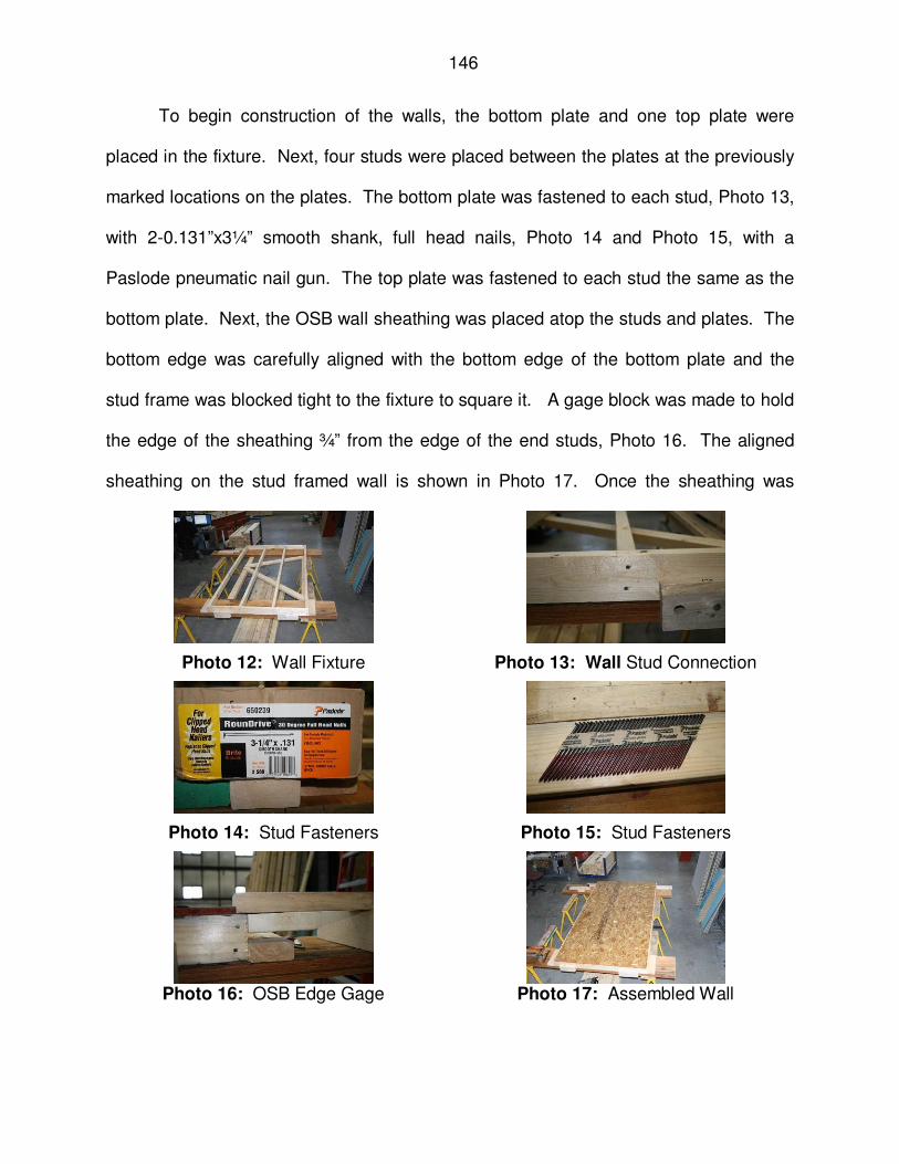
shown in Figure 12, Figure 13, and Figure 14 at the end of this chapter.
Group A walls were tested first to determine the hold down force. The average
hold down force was used to calculate the restraining force for Groups B to D. More
details of the test program are presented in Appendix A.
Graph 15: Correlation of Wall Strength to Specific Gravity
0
100
200
300
400
500
600
700
0.340 0.350 0.360 0.370 0.380 0.390
Average Specific Gravity of Wall Studs and Plates, G
Wall
Str
en
gth
, p
lf
Wall A Test Values
Adjusted APA 154
+σ
−σ
Figure 12: Test Assembly Wall A
71
Figure 13: Test Assembly Walls B, C and D
72
Figure 14: Test Assembly Wall E
73
74
CHAPTER 4
FINITE ELEMENT MODELING
A finite element model was created to offer a better understanding of the
behavior of the walls with varying restraint conditions. The model includes a nonlinear
finite element analysis. The load deformation curves are compared to the test results
for accuracy of the model.
4.1 Finite Element Model
The finite element model (FEM) was constructed in HYPERMESH and analyzed
in ABAQUS, a commercial finite element solver. The model was constructed to
replicate as much detail as possible of the walls tested. The model used:
• Beam elements for the framing members • Four node quadrilateral shell elements • Two orthogonal springs connecting framing members, one linear and one
nonlinear • Two uncoupled orthogonal nonlinear springs (or spring pair) connecting
the sheathing to the framing elements • Compression-only beam elements at the supports that cannot resist
tension • And a nonlinear spring for the hold down.
Initially, the model was constructed with a single 1D nonlinear spring element
that was free to rotate (a SpringA element in ABAQUS). However, this element created
difficulties solving. It was extremely difficult to obtain convergence in the early steps of
the analysis. ABAQUS had difficulty in these early steps as the springs rotated to their
initial displacement path. The uncoupled nonlinear spring pair overcame this difficulty
and created a model that was easier to converge during the initial steps.
75
The uncoupled nonlinear spring pair is a common model that is commonly found
in other literature (Cassidy 2002, Dolan and Foschi 1991, and Folz and Filiatrault 2001).
As stated in Chapter 2, the uncoupled nonlinear spring pair is sufficient for determining
the ultimate load and displacement for monotonic loading.
4.1.1 Elements
Figure 15: Finite Element Model
The FEM model is shown in Figure 15. A description of the actual elements used
in the ABAQUS software model follows. For more information regarding these
elements, please refer to the “ABAQUS Analysis User’s Manual” (ABAQUS 2010).
Nail element, 6:12 spacing.
V
P
2x2 shell element for sheathing, typ.
Compression only support beam element with pinned support, type.
Beam elements for studs
76
4.1.1.1 Framing Members
The framing members, studs and plates were modeled as type B31 two node
three-dimensional beam elements. This element uses linear interpolation. B31
elements have six degrees of freedom at each end. These elements can be defined by
different geometric shapes. For this model, a rectangular shape was used to model a
2x4 framing member.
The second top plate of the wall was fastened only to the first top plate of the
wall. This was deemed insignificant to the strength and stiffness of the wall since it was
not fastened to the sheathing. It is common for models in the literature (Cassidy 2002,
Judd 2005) to use both plates as one member of equal dimension. This would create
additional stiffness that does not exist for the walls tested in this research.
Material properties for the B31 element are defined in the material properties
card. The material properties used are explained in the Materials section of this chapter.
The length of the elements for the studs was 6” and the length of the elements
for the sole and top plate was 2”. These lengths worked well for the nail and framing
geometry and for the behavior of the wall as well.
4.1.1.2 Nails
The framing members were connected with two orthogonal springs (or spring
pair), one linear and one nonlinear, as shown in Figure 16. As noted earlier, these
springs are each one dimensional spring elements. These springs are modeled as
Spring2 elements in ABAQUS. The spring used for lateral movement, or shear, was a
linear spring while the spring used for end grain withdrawal was a nonlinear spring.
77
The sheathing was connected to the framing
members with two orthogonal springs (or spring pair) as
shown in Figure 16. As with the framing members these
were one dimensional spring elements modeled as
Spring2 elements in ABAQUS. This spring pair contains
uncoupled, nonlinear springs with equivalent properties.
As shown in Figure 16, the spring pair allows the
node to move from point 1 to point 1′. This allows a two dimensional movement of the
node replicating the nail displacement. As explained in Section 2.9.1, the spring pair
model provides correct results for peak load and displacement for monotonic loading.
The spring properties for these elements are explained later in Section 4.2.
4.1.1.3 Sheathing Members
The sheathing was modeled as four node quadrilateral shell elements. The
general purpose S4 element was used. This element has six degrees of freedom at
each node. The element size was 2” x 2” for ease of geometric construction. An
element size of 4” x 4” is acceptable to model the sheathing. Cassidy modeled 16”, 8”,
4” and 2” elements and found convergence with 4” elements. He also used 2” elements
to simplify the geometry for other nail patterns. (Cassidy 2002)
4.1.2 Materials
The material properties for the FEM were taken from available literature as well
as from data obtained from the test. The stud and plate properties were taken from the
NDS (2005) and the Wood Handbook (1999). Sheathing properties were taken from the
1
1′
Figure 16: Spring Pair
78
Plywood Design Specification (2004). Sheathing nail data and hold down data was
obtained from the test results for the Group A walls. Stud to framing nail data was taken
from the literature (Cassidy 2002).
Although wood is an orthotropic material, it is typically modeled as an isotropic
material for wood shear walls (Judd 2005, Cassidy 2002). For the elements used, the
modulus of elasticity and Poisson’s ratio were required. The following values were used
for the analysis:
Table 17: Framing Material
Material Sizea (in)
MOEa (psi)
Poisson’s Ratiob υ
Studs – SPF-S 1.5 x 3.5 1 x10⁶ 0.3
Plates – SPF-N 1.5 x 3.5 1.4 x 10⁶ 0.3 a From the NDS (2005) b Estimated from orthotropic properties (Wood Handbook 1999)
For compression only support members, the material properties for the studs
were used, but without tension. ABAQUS allows a “no tension” command to be added
to a material property. This command does not allow tension stresses to occur in that
material. Convergence of the model using this method worked better than using springs
to model these supports.
The OSB sheathing material properties were taken from the Plywood Design
Specification (2004). The following values were used for the analysis:
79
Table 18: Sheathing Material
Material Thicknessa
(in) MOEa
(psi) Shear Modulusa
(psi) Poisson’s Ratiob
υ 15/32” OSB 0.469 0.738 x10⁶ 0.178 x10⁶ 0.3 a From the PDS (2004) b From literature (Judd 2005)
4.2 Connections
The properties for the sheathing nail spring pairs are the one dimensional spring
element spring constants or the nonlinear load deformation nail curve data. The
nonlinear load deformation nail curve data was taken from the test results as explained
earlier in Section 3.3.1. The data was reciprocated in the negative region from the
positive data to provide the same stiffness in the event that the spring moved in the
negative direction. The same nail data was used for both orthogonal springs in the
spring pair.
The nail data from the test results, shown in Graph 10, were calibrated in the
model so the model behaved similarly to the test results for all five wall types. The
values used in the FEM are tabulated in Table 19 and they are also shown in Graph 16.
For comparison, the nail data from the test results of wall A are also shown in Graph 16.
In order to help with convergence, the stiffness at zero displacement is 5 lb. This
was chosen as a small value so the spring doesn’t have zero force at the beginning of
the analysis.
The properties for the stud to plate nail elements were also spring constants, or
the load deformation curve data. This connection also consists of two orthogonal
springs. The stiffness of the springs for this connection is not the same in both
80
Table 19: Sheathing Nail Data
Displacement (in)
Load (lb)
-1.500 -37
-1.000 -148
-0.720 -213 -0.540 -250
-0.369 -240
-0.180 -200 -0.042 -100
0.000 5
0.042 100 0.180 200
0.369 240
0.540 250 0.720 213
1.0 148
1.5 37
Nail Load Deformation Model
-300
-200
-100
0
100
200
300
-2.00 -1.50 -1.00 -0.50 0.00 0.50 1.00 1.50 2.00
Displacement, in
Lo
ad
, lb
Nail Data for Abaqus
Nail Data from Wall A Tests
Graph 16: Sheathing Nail Data for ABAQUS
81
directions. The two directions considered are perpendicular to the stud in the plane of
the wall and parallel to the stud in the plane of the wall. The latter is a withdrawal load
from the end grain of the stud. For the direction perpendicular to the stud, a linear
spring stiffness of 12,000 lb/in was used, which was used by Cassidy (2002) and
published by Dolan et. al. (1995). For the direction parallel to grain, a nonlinear spring
stiffness was used. The nonlinear spring stiffness was modified from the values used
by Cassidy (2002). The modification was made on the tension value due to
observations made during testing and dismantling the walls. It was observed that nail
withdrawal from the end grain of the stud was not linear. The connection remained
intact and then abruptly withdrew. The exact magnitude of this response is not known.
A parametric study was conducted with the FE model until the load deformation curve
reasonably met the test results. Recall that Cassidy (2002) used an arbitrary tension
stiffness of 100 lb/in. As noted above, the compression stiffness was not altered and a
value of 41,000 lb/in was used as modeled by Cassidy (2002). The values used in the
FEM are tabulated in Table 20 and they are also shown in Graph 17.
Table 20: Stud to Plate Vertical Nail Data
Displacement (in)
Load (lb)
-1.0 -41,000
0.0 5
0.094 200 3.0 450
In order to obtain convergence of the model, the spring pairs for the framing
member connections were used for the two studs closest to the leading edge only
(where tension will result). The other two studs were simply connected to the plate
5.2 Reliability of SDPWS Nominal Unit Shear Capacities
It is necessary to understand the reliability of the current unit shear capacities in
order to calibrate the partially restrained shear wall unit shear capacities. To
accomplish this, the origination of the SDPWS values was researched. The values in
SDPWS originate from APA Research Report 154.
The test results, shown in Table 12, indicate that a mechanical hold down device
at the bottom tension corner is not sufficient to achieve the fully restrained shear wall
capacity. Therefore, to determine the capacity of a fully restrained shear wall, the
values published in APA Report 154 were used and are indicated here for the 15/32”
99
WSP as used for the test samples. The nominal design unit shear capacity for 15/32”
WSP are based on the results of seven tests, Table 25. The seven test results are a
combination of three tests using 19/32” plywood and four tests using 5/8” plywood. The
panel thickness has little influence on the ultimate capacity of the shear wall (van de
Lindt and Rosowsky 2005). Therefore, it is reasonable to use the test results shown in
Table 26 as the ultimate unit shear capacity for 15/32” WSP.
Table 25: Excerpt from APA Report 154, Table A1
Fastener Ultimate Loads (plf)
Size Spacing
(in)
Panel Thickness(a)
(in)
No. of Tests Min. Max. Avg.
Target Design Shear
Load Factor(b)
RATED SHEATHING 8d 6 15/32 7 689 1033 913 260 3.5
(a) Minimum panel thickness for design shear, some walls sheathed with thicker panels. (b) The load factor is determined by dividing the average ultimate load by the target design shear.
A summary of the reported test results shown in Table 25 and Table 26 are
shown in Table 27. Since all four tests are not reported for the 5/8” WSP, the two missing
(a) The load factor is determined by dividing the average ultimate load by the target design shear. (b) Design shear increased for “over-thick” panel, studs 16” o.c. or panel placed with 8’ length
perpendicular to framing.
100
Table 27: Summary of APA Report 154
950992
1033689
1000863.5 1
863.5 1
Average 913Standard Deviation 119COV 0.131Estimated from data in APA Report 154.
Ultimate Capacity
(plf)
19/32
Panel Thickness (in)
5/8
The standard deviation and distribution of the APA wall tests are needed to
calculate the reliability of SDPWS. Table 27 includes one of these two parameters.
The distribution is expected to be lognormal as found with the test results reported in
Section 3.3.4. To verify the accuracy of the COV in Table 27, it was compared with the
5% lower exclusion value for the data from APA Report 154. Table 28 shows that the
calculated standard deviation is very close to the 5% lower exclusion value. Since the
5% lower exclusion value is commonly used for timber design values, the actual
standard deviation of ultimate unit shear capacity from the APA test data is more
accurately 112 plf.
101
Table 28: Comparison of SDPWS Nominal Unit Shear to the 5th Percentile
Average 913 913COV 0.130 0.123Standard Deviation 119 112
5th Percentile 718 728
APA Data + 2 Estimated
Points
Values to Match
SDPWS
5.2.1 Reliability Model
The reliability model begins with the limit state equation. A basic limit state
equation is given in Eq. 11 which is repeated here. Failure occurs when g(x) <0. This
results in the basic design equation shown in Eq. 15. The load factors are given in
ASCE 7 (2005).
g(x) = R-S Eq. 11
Eq. 15
Where,
Rn = Nominal Strength for a Given
Failure Mode
Qn = Nominal Design Load
φ = Resistance Factor
γ = Load Factor
Since R and S are random variables, or multiple random variables, statistical
parameters must be known for each. The distribution function must be known. For the
distributions used in this thesis, two statistical parameters, the mean and the standard
∑=
γ≥φm
1iniin QR
102
deviation, are needed. Additionally the random variables must be identified. The wind
load, the shear wall strength, the dead load restraining force, and the specific gravity of
the framing lumber have been identified as random variables. Of these four random
variables, the parameters are known for wind load (van de Lindt and Rosowsky 2005),
the dead load (Ellingwood, et al 1980), and the specific gravity (ASTM D2555). The
parameters for the shear wall unit shear strength were determined from the wall testing
presented in this thesis. Table 29 summarizes the parameters known thus far.
Table 29: Summary of Distributions
Item nXX
vx (cov) DF Dead Load 1.05 0.1 Normal
Wind Load 0.8 0.35 Type 1 Specific Gravity, G 1.0 0.11 Lognormal2
Shear Wall Capacity Unknown Varies3 Lognormal3 1From ASTM D 2555 2From specific gravity test of lumber from samples
3From shear wall test results
The formation of the limit state function, g(x), then includes the unit shear
strength of the shear wall, V, the specific gravity of the framing lumber, G, the wind load,
VW, and the dead load, P. For the limit state of shear:
103
Eq. 16
Eq. 17
Eq. 18
Eq. 18 shows the relationship of the average shear load to the bias factor,
resistance factor, load factor, and the nominal unit shear strength.
5.2.2 Reliability Analysis Results
Since the SDPWS shear wall is considered as fully restrained, only two of the
four random variables are considered to determine the reliability of the SDPWS unit
shear capacity. The two random variables are the wall shear strength and the wind
load. These two random variables were applied to Eq. 11. Using the first order second
moment, FOSM, reliability method the reliability index β was determined to be 3.27 for
the 15/32” shear wall tabulated in SDPWS for a fully restrained condition. Recall from
Section 2.6 that the SDPWS values are 2.8 times the APA Report 154 target design
shear. Therefore, as determined by the quotient of the average ultimate load, 913 plf, in
)).(( G501VV tabn −−=
un VV ≥φ
nWWu VVV φ=γ=
W
nW
VV
γ
φ=
W
n1W1W
VaVaV
γ
φ==
load shear V
windto due load shear UnfactoredV
factor bias load a
gravitySpecific
values shear unit SDPWS
Where,
W
W
1
Average
Wind
G
Vtab
=
=
=
=
=
104
Table 25 and the nominal unit shear capacity, 730 plf, in SDPWS, Table 6, the bias
factor used in SDPWS is 1.25. The calculations are shown in Appendix D.
The target reliability index, β, for the calibration of the partially restrained shear
walls tested will be 3.25 since the SDPWS nominal unit shear capacity has a reliability
index of 3.27. This is reasonable based on other literature (van de Lindt and Rosowsky
2005).
5.3 Base Calibration of Partially Restrained Unit Shear Capacities
The reliability index of the unit shear capacity of the unrestrained shear wall was
calculated next. Using the mean unit shear capacity of wall E, 162 plf, from Table 12,
the reliability index was calculated using the FOSM method. The calculations are
shown in Appendix E for a bias factor of 1. With a bias factor of 1, the reliability index,
β, was determined to be 2.59, Table 30. The calculations were iterated changing the
bias factor, Table 30, and the results were plotted in Graph 28. The calibrated bias
factor was determined from the graph and verified again with calculation. A summary of
the results is shown in Table 30.
This procedure was repeated for the remaining partially restrained walls A, B, C,
and D. A summary of the results are shown in Table 31. Note that the calibrated
values shown in Table 31 simply calibrate all of the partial restraint conditions from the
tests and the SDPWS (APA) values to the target reliability index, β=3.25. This is
appropriate for the ASD load combination D+W with a safety factor, Ω=2.0. For the
mechanical hold down, Group A walls, the unrestrained Group E walls, and the SDPWS
105
(APA) fully restrained wall, this is also appropriate for the LRFD load combination
1.2D+1.6W with a resistance factor, φ=0.8.
Table 30: Nominal Unit Shear Calibration for Unrestrained Wall E
V(Strength) Vw(Load)
uVN aV uV σV uVwN aVw uVw σVw
plf plf Plf plf plf plf
β
162.0 1.00 162 23.5 81.0 0.8 64.8 22.7 2.59
154.3 1.05 162 23.5 77.1 0.8 61.7 21.6 2.72
147.3 1.10 162 23.5 73.6 0.8 58.9 20.6 2.84
140.9 1.15 162 23.5 70.4 0.8 56.3 19.7 2.96
135.0 1.20 162 23.5 67.5 0.8 54.0 18.9 3.07
129.6 1.25 162 23.5 64.8 0.8 51.8 18.1 3.19
126.6 1.28 162 23.5 63.3 0.8 50.6 17.7 3.25
124.6 1.30 162 23.5 62.3 0.8 49.8 17.4 3.3
120.0 1.35 162 23.5 60.0 0.8 48.0 16.8 3.39
115.7 1.40 162 23.5 57.9 0.8 46.3 16.2 3.49
111.7 1.45 162 23.5 55.9 0.8 44.7 15.6 3.59
108.0 1.50 162 23.5 54.0 0.8 43.2 15.1 3.69
104.5 1.55 162 23.5 52.3 0.8 41.8 14.6 3.78
The reason that the nominal unit shear values shown in Table 31 are appropriate
for the ASD and LRFD load combinations stated is that the dead load will not affect the
wall strength in these load combinations. There are additional load combinations (Table
24) which require a reduced load factor for the dead load. This insures that dead load
will not be a limiting factor and these combinations are addressed in section 5.4.
Therefore, the unit shear capacity of the wall is the only random variable on the strength
side considered for this step.
To illustrate the relationship between partial restraint and nominal unit shear
strength, the results shown in Table 31 are graphed in Graph 29. Note that the shape
of the graph is similar to Graph 12. The difference between these two graphs is shown
in Graph 30. Note that the fully restrained wall has 100% unit shear capacity in both the
106
0
20
40
60
80
100
120
140
160
180
2.5 2.75 3 3.25 3.5 3.75 4 4.25 4.5
No
min
al U
nit
Sh
ear
Str
en
gth
, p
lf
Reliability Index, ββββ
Wall E - Unrestrained
Graph 28: Calibration of Unrestrained Shear Wall
nominal, calibrated, the ultimate and test result. They are the same due to the
normalization. The unrestrained wall is nearly the same as well. The larger difference
occurs for walls B, C, and D. This difference is due to the shift in the percent of full
restraint. The mechanical hold down cannot achieve the same unit shear capacity as a
wall restrained from the top. This was discussed in Section 3.3.3. The difference in the
two points in Graph 30 is from the calibration as well as the percent of full restraint
Graph 29: Partial Restraint Effect on Strength - Calibrated
108
0%
20%
40%
60%
80%
100%
120%
0% 20% 40% 60% 80% 100% 120%
% o
f F
ull S
he
ar
Ca
pa
cit
y
% of Full Restraining Force
Test Data + APA
Holdown
Pure test results(uncalibrated)
Pure Test(uncalibrated)
Poly. (Test Data + APA)
Poly. (Pure test results(uncalibrated))
Graph 30: Comparison of Calibrated Partial Restraint Effect
5.4 Extended Calibration of Partially Restrained Unit Shear Capacities
5.4.1 Calibration with Reduced Dead Load Combinations
Next, the unit shear capacities were calibrated for the ASD and LRFD load
combinations that have a dead load factor, γD, less than 1. This is a critical part of the
calibration to consider since the partially restrained shear walls use a dead load applied
to the top of the wall to resist the lateral wind load.
5.4.2 Calibration without a Variation in the Specific Gravity
First, the calibration was performed without considering the specific gravity of the
framing lumber as a random variable. The random variables for this calibration are the
109
unit shear capacity, V, the wind load, VW, and the dead load, P. These random
variables are defined in Table 29.
The shear wall ultimate unit shear capacity is a function of the restraining force.
As shown in Eq. 14, the ultimate unit shear capacity of a partially restrained shear wall
is related to the fully restrained shear wall unit shear capacity by the partial restraint
factor, Cpr-u. This relationship was used for the second calibration. Since the restraining
force, PD, is a random variable, then Cpr-u varies. However, Cpr-u cannot be greater than
1. This limit cannot be accounted for in a FOSM model. Therefore, for the second
calibration, a Monte Carlo simulation was used.
The Monte Carlo simulation was conducted in Excel 2010. To adequately capture
the target reliability index, β, of 3.25 (pf = 5.77e-4), four million simulations were used.
This was done by repeating 100,000 simulations 40 times for each increment of bias
factor studied. The calibration consisted of varying the bias factor to achieve the target
reliability index, β=3.25; similar to what was done with the first calibration with the test
data. The results were graphed to determine the calibrated bias factor similar to Graph
28. The value from the graph was then confirmed with 4 million simulations. The Monte
Carlo simulation is described below.
5.4.3 Random Variables used for Calibration
The nominal shear capacity of the wall is:
110
or,
Since V is a random variable, Vn is a random variable as well. For this step, the
specific gravity, G, is considered a constant.
Recall from Eq. 14 that the partially restrained unit shear capacity is the fully
restrained unit shear capacity modified by the partial restraint factor (Eq. 13) which is
repeated here:
Cpr-u = -0.6393λ2+1.4331λ+0.206 ≤ 1.0 Eq. 13
height wallshearh
capacity shear unit ultimate averageV
variable) (random force grestraininP
hV
P
ult
D
ult
D
=
=
=
×=λ
Therefore,
Eq. 19
2
n
aV
V=
factor biasCapacity Sheara
Where,
2 =
2
na
VV =
( )( )
2
na
G501VV
−−=
.
( )( )
2
upr
na
G501VCV
−−=
− .
111
The mean dead load restraining force applied to the wall is:
Adding the load factor:
Eq. 20
The nominal wind load is taken as the nominal capacity of the shear wall.
Therefore, the nominal wind load is calculated as shown here:
Eq. 21
or,
Eq. 22
3
n
Da
P
P=
factor load Dead
factor bias load Deada
Where,
D
3
=γ
=
D3D PaP =
D
D3D
PaP
γ=
W
nnW
VV
γ
φ=
nWW VaV 1=
W
n1W
VaV
γ
φ=
factor load Wind
factor resistance
factor bias load Winda
variable) (random shear unit load windmeanV
variable) (random shear unit load windminalnoV
Where,
W
1
W
Wn
=γ
=φ
=
=
=
112
And, for a partially restrained shear wall, the limit state equation is:
Eq. 23
5.4.4 Random Variable Distributions
Although Eq. 23 only indicates two random variables, keep in mind that there is a
third random variable, PD, included in the partial restraint factor, Cpr-u. Table 34
summarizes the three random variables necessary for Eq. 23 and the Monte Carlo
simulation. The bias factor for V is indicated as “unknown” because this is what is being
determined by the calibration.
Table 32: Summary of Distributions
Random Variable Item nX
X vx (cov) DF
PD Dead Load 1.05 0.1 Normal
VW Wind Load 0.8 0.35 Type 1
V Shear Wall Capacity
Unknown 0.123 Lognormal4
1From ASTM D 2555 2From specific gravity test of lumber from samples 3From Table 28 4From shear wall test results
5.4.5 Steps used for Monte Carlo Simulation
The Monte Carlo simulation was conducted with the following steps:
1. Begin with the restraining force. This is the restraining force from walls B, C, and
D; 1104 lb, 2208 lb, and 3312 lb respectfully.
a. Calculate the mean dead load restraining force, DP , using Eq. 20 and its
bias factor shown in Table 32.
( ) WW VVVVg −=,
wallthe ofcapacity shear unit V
shear unit load windV
Where,
W
=
=
113
2. Calculate the partial restraining factor, Cpr-u, Eq. 13 using the restraining force
from step 1.
3. Determine the mean ultimate unit shear strength, V , from APA Report 154, and
its statistical properties.
4. Start with a trial bias factor, a2=0.8.
5. Calculate the nominal unit shear strength, Vn, using Eq. 19, with the specific
gravity of the wall framing members, G=0.36 for SPF –S.
6. Calculate the nominal wind load, VWn, using Eq. 21.
7. Calculate the mean wind load, WV , using Eq. 22 and its statistical properties.
8. Monte Carlo Simulation
a. Use a random number generator to generate a random probability
between 0 and 1 and calculate the inverse of the CDF (normal distribution)
for the dead load, PD, at the random probability.
b. Using the result of step 8.a, calculate Cpr-u using Eq. 13.
c. Use a random number generator to generate a random probability
between 0 and 1 and calculate the inverse of the CDF (lognormal
distribution) for the unit shear capacity, V, at the random probability.
d. Calculate the partially restrained unit shear capacity of the wall by
modifying the unit shear capacity, V, from step 8.c by the partial restraint
factor, Cpr-u, from step 8.b.
e. Use a random number generator to generate a random probability
between 0 and 1 and calculate the inverse of the CDF (Type I extreme
value distribution) for the wind load, VW, at the random probability.
f. Using Eq. 23 calculate the survival of the function (g(x)>0 for survival).
Set a flag equal to zero for survival or one for failure.
g. Repeat steps 8.a to 8.f 100,000 times, and add the number of failures in
step 8.f.
9. Repeat step 8 forty times and sum the total number of failures from step 8.g.
Calculate the reliability of the 4,000,000 samples and then calculate the reliability
index, β as shown:
114
)R(
R
pR f
−Φ=β
−=
−=
− 1
4,000,000
failures of #1
1
1
10. Plot the bias factor, a2, and the reliability index, β, from step 9.
11. Increase the bias factor, a2, increment (0.1 was used) and repeat steps 5 to 11
until 253.≥β .
12. Using the graph from step 10, determine the correct bias factor, a2, to obtain the
target reliability index β=3.25.
13. Repeat steps 5 to 9 to validate the bias factor, a2, determined in step 12.
14. Make correction to the bias factor a2 if necessary and repeat steps 5 to 9.
15. Repeat entire procedure for next wall set (restraining load).
An illustration of the Excel spreadsheet used for the Monte Carlo simulation is
shown in Appendix F.
5.4.6 Calculations for Monte Carlo Simulation
The known distributions of each random variable were used in the MCS to
generate random values to evaluate Eq. 11. As shown in Table 32 and again in Table
34, three distributions were used, Normal, Log-Normal, and Type I. The cumulative
distribution function, CDF, for each of these was used along with a random number
generator to generate values of the random variables. The random number generator is
used to generate a probability which can then be evaluated with the CDF to determine
the random variable value at the generated probability.
115
For normal distribution, denoted as N(µ, σ), the PDF is given as:
Where, µ=mean of the variate σ=standard deviation of the variate
The CDF is then given as the integral of the PDF and is commonly referred to as
FX(x). The CDF, FX(x), is given as:
Where, FX(x)=the probablity that -∞ < X ≤ x µ=mean of the variate X σ=standard deviation of the variate X
For the standard normal distribution, denoted as N(0,1), the CDF is commonly
noted as FS(s) = Φ(s). And the value of a standard normal variate at a cumulative
probability, p, is Φ−1(s). Φ(s) and Φ−1(s) are commonly tabulated. With the use of the
table of Φ(s), probabilities can be easily determined for any normal distribution by
substituting:
As described above for a standard normal variate, for a given probability, any
normal variate can be determined using:
σ
µ−−
πσ=
2
2
1
2
1 xexp)X(fX ∞<<∞− x
( ) dx∫
∞−
σ
µ−−
πσ=
x
X
xexpxF
2
2
1
2
1
σ
µ−=
xs
)x(x 1−Φ=
σ
µ−
116
Therefore, for any given probability, Φ(x), the value of x can by calculated. A
random number generator is used to generate the probability Φ(x) for which a given
value for the random variate X is calculated using Φ-1 (x). Therefore, if p is a random
probability, Φ(x), the value of the random variate is calculated as:
Where, p= probability that -∞ < X ≤ x, and is randomly generated µ=mean of the variate X σ=standard deviation of the variate X
The use of this for the MCS is illustrated in Appendix F.
For lognormal distribution, the PDF is given as:
Where,
The parameters λ and ζ are related to the mean µ and the standard deviation σ
of the variate as (Ang and Tang, 1975):
ζ
λ−−
ζπσ=
2
X
x
2
1
x2
1xf
lnexp)( ∞<≤ x 0
)(ln
)(ln
XVar
XE
=ζ
=λ
µ
σ+=ζ
ζ−µ=λ
2
22
2
1
2
1
ln
ln
µ+σ=
=Φ
Φ=
=≤<−∞
−
sx
on,distributi normal standard
the for tabulated is CDF the Since
1 x)p(
)x(p
p)xX(P
117
If σ/µ is ≤ 0.30, then,
The CDF is then given as the integral of the PDF and is given as:
Where, P=the probability that X is between a and b λ=mean of the lognormal of the variate X ζ=standard deviation of the lognormal of the variate X
The lognormal distribution of a random variable X is a normal distribution of the
natural logarithm of X. Therefore, the commonly tabulated values of Φ(s) and Φ−1(s) for
standard normal distribution can be used similarly to the description earlier where:
And also similar to the explanation above for normal distribution, for a given
probability, the normal variate can be determined using:
Therefore, for any given probability, Φ(x), the value of x can by calculated. A
random number generator is used to generate the probability Φ(x) for which a given
value for the random variate X is calculated using Φ-1 (x). Therefore, if p is a random
probability, Φ(x), the value of the random variate is calculated as:
µ
σ≈ζ
dx∫
ζ
λ−−
ζπσ=≤<
b
a
2x
2
1
x2
1bXaP
lnexp)(
ζ
λ−=
xs
ln
)x(xln 1−Φ=
ζ
λ−
118
Where, p= probability that -∞ < X ≤ x, and is randomly generated λ=mean of the lognormal of the variate X ζ=standard deviation of the lognormal of the variate X
The use of this for the MCS is illustrated in Appendix F.
For the Gumbel Type I distribution, the CDF is given as Eq. 9 and is repeated
here:
( ) ( )( )[ ] ∞<<∞−−α−−= xuxexpexpxF nXn Eq. 9
Where, un = location parameter αn = scale parameter
The location and scale parameters are related to the mean and standard
deviation of the random variable X as:
n
xn
x
n
u
6
α
γ−µ=
σ
π=α
Where,
αn = scale parameter un = location parameter σx = standard deviation of random variable X
µx = mean of random variable X γ = Euler’s Constant = 0.577216
( )λ+ζΦ=
=Φ
Φ=
=≤<−∞
−
−
)x(exp
x)p(
)x(p
p)xX(P
1
1
x
on,distributi normal standard
the for tabulated is CDF the Since
119
Since the CDF is given directly in Eq. 9, the probability that -∞ < X ≤ x is FXn(x).
Eq. 9 can be rearranged, Eq. 24, to solve for the value of x at a random probability:
( )( )[ ] 1xFlnlnux
nX
n
n −α
−= Eq. 24
Where, un = location parameter αn = scale parameter FXn
(x) = probability of Xn, and is randomly generated
The use of this for the MCS is illustrated in Appendix F.
5.4.7 Results of the Monte Carlo Simulation for ASD
The results of the MCS for the ASD load combination 0.6D+W are summarized in
Table 33 for wall Groups A, B, C, D, E, and SDPWS. The values for A, E, and SDPWS
are from the FOSM analysis summarized in Table 31. For these walls, the restraining
force was not the limit state of failure and was not modeled in the MCS. The ASD load
combination will assure there is enough dead load for these conditions.
Table 33 summarizes the restraining force, the average unit shear capacity from
the test results and SDPWS, the bias factor from the calibration, and the resulting
nominal unit shear capacity. The nominal unit shear capacity was then normalized to
the SDPWS nominal unit shear capacity. Similarly, the ratio of the restraining force to
the SDPWS restraining force was also tabulated to achieve the nominal unit shear
capacity.
120
Table 33: Summary of MCS for ASD without Specific Gravity
The results are only slightly different from the curve shown in Graph 33 without
the added random variable, G. An additional second order curve was fit for comparison
to the B-N fit. The resulting curve has an R2 value of 0.9999. The equation for the
second order curve is simpler than that of the B-N curve and is presented in Eq. 33.
130
Since the LRFD calibration curve shown in Graph 34 resembles the actual
behavior of the actual test walls and since Eq. 33 is simpler than Eq. 32, LRFD is the
preferred method for design. The partial restraint factor in LRFD will make more sense
to the building designer. The calculation of the partial restraint factor is also easier for
the building designer.
y = -0.4807x2 + 1.2716x + 0.2081R² = 0.9999
0%
20%
40%
60%
80%
100%
120%
0% 20% 40% 60% 80% 100% 120%
% o
f F
ull S
hea
r C
ap
acit
y
% of Full Restraining Force
Holdown
Monte Carlo w/ G
B-N w/ G
2nd Order Fit
Second Order Fit
Graph 34: Partial Restraint Effect, LRFD, with Specific Gravity
Partial Restraint Factor for 0 ≤ λ’ ≤ 1,
208027214810 2 ...C 'npr +λ+λ−=−
For λ’>1,
Cpn-n = 1.0
Eq. 33
131
CHAPTER 6
DISCUSSION OF NOMINAL UNIT SHEAR VALUES
This chapter addresses some of the conflicts that exist with current methods of
determining unit shear values for wood structural panels. These conflicts directly relate
to the capacity of a partially restrained shear wall as prescribed in the IRC (2009).
6.1 Difference in Method to Determine Unit Shear Values
6.1.1 SDPWS Values for Anchoring Device
The SDPWS (2005) unit shear values, based on APA Research Report 154
(APA 2004) cannot be achieved with a conventional mechanical hold down only. The
values are reportedly based upon ASTM E72. The test frame from ASTM E72 is shown
in Figure 22. The clamping action of the test fixture is not equivalent to applying a
conventional hold down on the tension stud as explained earlier.
APA Research Report 154 (APA 2004) indicates that a timber was used over the
top of the wall and a double tie rod hold down was used to restrain the tension side of
the wall. The double tie rod system over the top of the wall provides a clamping force
keeping the wall plates in contact with the wall stud. This action keeps the plates and
stud from separating, thus reducing the force on the corner nails at the tension side.
Additionally, the second stud at each end adds additional strength and stiffness even
though the sheathing is not directly attached to it.
The conventional mechanical hold down attached to the tension stud does not
offer the same restraint as the clamping mechanism required by ASTM E72. The
elongation of the mechanical hold down allows the tension stud to separate from the
132
bottom plate and there is nothing to keep the top plate from separating from the tension
stud unless additional building framing exists. The result is the capacity of the wall is
reduced. This was observed in the test specimens and was also observed in the FE
model.
Reprinted, with permission, from ASTM E72-10 Standard Test Methods of Conducting Strength Tests of Panels for Building Construction, copyright ASTM International, 100 Barr Harbor Drive, West Conshohocken, PA 49428.
Figure 22: ASTM E72 Test Fixture
SDPWS (2005) requires either a dead load stabilizing moment or an anchoring
device at the end of the shear wall. No difference is given to either restraining device.
There is a difference between the two; the resulting unit shear strength based on the
test results shown in Table 12 with an anchoring device is 13% less or 87% of the
133
tabulated nominal unit shear value published in SDPWS (2005). Therefore, SDPWS
(2005) should at least provide an anchoring device factor, Ca, as given in Eq. 34. This
value should not be confused with the value determined in Chapter 5 which was
calibrated for design. The latter is preferred since it was calibrated to ASCE 7-05 and
the IBC (2009) load combinations to provide a reliability index, β, of 3.25.
Ca = 0.87
Eq. 34
6.1.2 Use of ASTM E72
One of the intentions of ASTM E72 is to provide a test method and a test frame
that can be used to compare different sheathing materials for use as shear walls to
resist lateral forces, such as wind loads. The standard states that it intends to function
as a shear wall that would typically be used in a building. The purpose of the standard
is to provide a relative comparison of sheathing materials.
While the stated intent of the standard is good and useful, the standard does not
capture the behavior of partially restrained shear walls that are prescribed in the 2009
IRC. It has been explained earlier that there is a large difference between a fully
restrained shear wall and a wall only restrained in accordance with the 2009 IRC.
These differences are not tested and the resulting behavior is not captured in ASTM
E72.
Due to the increased forces in the corner nails in a partially restrained shear wall,
as well as shear walls having no dead load along the top of the wall restrained with a
hold down, wall sheathing intended as shear wall material should be tested to capture
134
this behavior. This will provide a relative comparison of different materials. The
behavior of the sheathing material at the edges can be crucial to the strength of the wall
and in fact was the focus of the research conducted by Cassidy (2002).
ASTM E72 recognizes that a prestress force can greatly influence the results of
the racking test and restricts the prestress in the hold down rods to 20 lb. However,
there is no requirement to report the initial hold down force or the hold down force
throughout the test. Reporting of this data should be made so that the entire test
method to determine the resulting unit shear values is completely transparent if these
values will be used in design standards. This too will allow for a comparison of different
sheathing materials.
6.1.3 Use of ASTM E564
ASTM E564 states that its use is not intended for classifying sheathing shear
capacity. Thus, to this author’s knowledge, it is not used in the design standards. In
contrast to ASTM E72, ASTM E564 allows for walls to be constructed in dimensions
intended for use and with the boundary conditions and restraining forces of the intended
use. This results in data that reflects the actual construction of the wall and doesn’t
attempt to only make a relative comparison of sheathing material shear capacity as
ASTM E72 does.
Since the failure of wood shear walls is highly dependent on the capacity and
response of the fasteners as well as the initial boundary conditions, it makes sense to
use ASTM E564 for codified design standards for partially restrained wood shear walls.
This standard was used as the basis of the testing for this thesis as well. This would
135
also provide a relative comparison of sheathing material performance where edge
breakout or failure is the limit state.
6.1.4 Partial Restraint Factors
It is obvious that the peak capacity of wood shear walls in a fully restrained
condition is greater than the peak capacity of a wood shear wall with a mechanical hold
down at the base of the wall. Therefore, when a wall is partially restrained from the top,
the partially restrained capacity must be a function of the fully restrained condition (i.e.
the APA Research Report 154 ultimate capacity) rather than the nominal (SDPWS –
unless it is calibrated) capacity, or the mechanical hold down restrained capacity. This
is best shown in Graph 35 where the partial restraint effect from this research is
compared with Ni and Karacabeyli’s (2000).
As explained earlier in Chapter 2, Ni and Karacabeyli (2000) assumed that a wall
with a mechanical hold down at the base of the wall was fully restrained. As shown in
Graph 35, there is a noticeable difference when using this assumption. The light scale
represents Ni and Karacabeyli’s (2000) partial restraint factor and partial restraint force.
Their curve was scaled to the hold down capacity from this research to make the
comparison.
Another problem with using the unit shear capacity developed with a mechanical
hold down as the fully restrained unit shear capacity is that this capacity is unknown
unless testing is conducted or unless a partial restraint factor for a mechanical hold
down is used as proposed in this research. Therefore, a correlation must always be
made to between the unit shear capacity with a mechanical hold down and the nominal
value in SDPWS (2005).
136
0%
20%
40%
60%
80%
100%
120%
0% 20% 40% 60% 80% 100%
% o
f F
ull S
hear
Cap
ac
ity
% of Full Restraining Force, λλλλ
Partial Restraint Effect on Strength
Test Data + APA
Holdown
SDPWS Nominal
Ni and Karacabyli
Poly. (Test Data + APA)
20% 40% 60% 80% 100%
20%
40%
60%
80%
100%
Graph 35: Comparison of Partial Restraint
137
CHAPTER 7
SUMMARY, CONCLUSION, AND RECOMMENDATIONS FOR FUTURE RESEARCH
7.1 Summary
The unit shear capacity of partially restrained WSP shear walls constructed in
accordance with the 2009 IRC was studied in this thesis. A nonlinear finite element
model was developed to understand and describe the behavior of these walls.
Additionally, as a focus of this thesis, a reliability analysis was conducted to develop
modification factors to fully restrained unit shear capacities. These modification factors
were calibrated to provide a uniform reliability index of 3.25.
7.2 Conclusions
The following conclusions are made from this research effort:
1. The SDPWS (2005) nominal unit shear capacity, 730 plf, for 15/32” WSP with
8d common nails at 6” o.c. at the perimeter and 12” o.c. at the intermediate
members provides a reliability index, β=3.25, for wind load using the ASD
reduction factor of 2 per SDPWS (2005) and using the LRFD resistance factor
of 0.8. This was used as the target reliability index for the calibration.
2. The derivation of design values for use in SDPWS with ASTM E72 is not
appropriate for walls anchored with mechanical hold downs or partially
restrained IRC (2009) prescriptive walls. The ASTM E72 test frame provides
a clamping action not present in partially restrained shear walls. ASTM E564
is appropriate for shear walls with these types of restraint.
138
3. ASTM E72 should add a requirement to record the initial and resulting hold
down force for a racking test. Though it has a limit of a maximum 20 lb of
initial hold down force, it does not have to be measured for the test.
4. The SDPWS (2005) nominal unit shear capacities, based on APA Research
Report 154 (APA 2004), cannot be achieved with a conventional mechanical
hold down at the base of the wall for a 4’ x 8’ WSP shear wall.
5. For the ASD design methodology, partially restrained shear walls have an
allowable nominal unit shear capacity to resist wind load, V’n, as shown in
Eq. 35. This is applicable to 4’ x 8’ WSP shear walls constructed in
accordance with the IRC (2009) using a mechanical hold down device (i.e.
Simpson HUD14) at the base of the wall.
ASD
Gan'
nC
CCVV =
Where,
Vn = nominal unit shear capacity per SDPWS (2005) Ca = anchor reduction factor Ca = 0.77 CG = 1-(0.5-G) G = specific gravity of the framing lumber CASD = 2
Eq. 35
6. For the ASD design methodology, wood shear walls partially restrained by a
dead load restraining force, P, have a nominal unit shear capacity to resist
wind load, V’n, as shown in Eq. 36. The controlling IBC (2009) load
combination is 0.6D+W. This is applicable to 4’ x 8’ WSP shear walls
constructed in accordance with the IRC (2009).
139
ASD
Gprn'
nC
CCVV =
Where, Vn = nominal unit shear capacity per SDPWS (2005)
2070163064210 09709257.)C..(C ..
ppr ++= −−
CG = 1-(0.5-G) G = specific gravity of the framing lumber
01C 01
0C 2070
01C0 hCV
P
p
p
p
Gn
.;.C
;.C
.;C
p
p
p
≥=
==
≤<=
h = height of shear wall P = 0.6PD [per IBC (2009)] (restraining force) CASD = 2
Eq. 36
7. For the LRFD design methodology, partially restrained shear walls have an
allowable nominal unit shear capacity to resist wind load, φV’n, as shown in
Eq. 37. This is applicable to 4’ x 8’ WSP shear walls constructed in
accordance with the IRC (2009) using a mechanical hold down device (i.e.
Simpson HDU14) at the base of the wall.
Gan
'
n CCVV φ=φ
Where,
φ = strength reduction factor φ = 0.8 Vn = nominal unit shear capacity per SDPWS (2005) Ca = anchor reduction factor Ca = 0.77 CG = 1-(0.5-G) G = specific gravity of the framing lumber
Eq. 37
8. For the LRFD design methodology, wood shear walls partially restrained by a
dead load restraining force, P, the nominal unit shear capacity, φV’n, as
shown in Eq. 38. The controlling IBC (2009) load combination is
140
0.9D + 1.6W. This is applicable to 4’ x 8’ WSP shear walls constructed in
accordance with the IRC (2009).
Gprn'n CCVV φ=φ
Where, φ = strength reduction factor φ = 0.8 Vn = nominal unit shear capacity per SDPWS (2005)
208027214810 2 .C.C.C pppr ++−=
CG = 1-(0.5-G) G = specific gravity of the framing lumber
01C 01
0C 2080
01C0 hCV
P
p
p
p
Gn
.;.C
;.C
.;C
p
p
p
≥=
==
≤<=
h = height of shear wall P = 0.9PD [per IBC (2009)] (restraining force)
Eq. 38
9. The curve generated by the partial restraint factor, Cpr, in Eq. 38 (LRFD
method) more accurately emulates the actual shear wall behavior than the
same factor in Eq. 36 (ASD method). The ASD controlling load combination
creates a shift in the curve of the partial restraint factor due to use of only
60% of the dead load restraining force.
10. The IRC (2009) assumption that shear walls are partially restrained requires a
dead load force applied to the top of the shear wall at the tension side as
indicated in Table 38.
Table 38: Design Restraining Force for IRC Shear Wall
Wall Supporting IRC Partial-Restraint Factor
Dead Load Required (lb)1
Roof Only 0.8 2,786 Roof + One Story 0.9 3,512
Roof + Two Stories 1.0 6,867 1Based on 3/8” WSP per IRC with SPF Framing, G=0.42
141
11. The clamping force in shear walls constrained from the top with either
external mechanical methods or dead loads allows a substantial horizontal
load to transfer through the studs to the plate (220 plf for this research). For
this reason, the nails in the vertical end studs always failed first for these
types of shear walls. This behavior is not realized without the clamping
action.
12. Finite element analysis should model the behavior of wood shear walls. It
should always include the effect of the boundary conditions and should model
the connection behavior of the studs to the plates. The separation of the
studs from the plate can greatly reduce the unit shear capacity of the wall.
7.3 Recommendations for Future Research
Future research could extend in a number of directions. Since the coefficient of
variation for wind load is so large, this is an area that could use further research.
Additional research could be conducted on the effect of wall length on partially
restrained walls. This could be included as a parameter to the partial restraint
modification factor if it is found to be significant. Finite element modeling could be
improved with further research on connections within the shear wall. Particularly the
interaction of nail withdrawal and shear resistance of the framing nails. Upon improving
the connection behavior in FEM, comparisons of whole building tests utilizing partial
restraints can be made and the FEM can be further calibrated.
142
APPENDIX A
WALL TESTS
A1 Wall Testing
This appendix details further the testing procedure conducted for the 25 wood
shear wall tests.
A2 Wall Materials
The material was delivered to the lab on March 11, 2011. The following material
G 0.57 0.64 0.60 0.61 0.55t, in 0.547 0.531 0.515 0.527 0.516
Set "E" with no Restraint
Member
Wall
OSB
170
APPENDIX B
SBCRI ACCREDITATION CERTIFICATE
171
172
APPENDIX C
STRING POTENTIOMETER AND LOAD CELL SPECIFICATIONS
173
174
175
176
APPENDIX D
FOSM RELIABILITY OF SDPWS
177
178
179
180
181
182
APPENDIX E
FOSM RELIABILITY OF WALL
183
184
185
186
187
APPENDIX F
MONTE CARLO SIMULATION
18
8
189
APPENDIX G
EXAMPLE CALCULATIONS OF UNIT SHEAR
This appendix illustrates the use of the proposed partial restraint factor. Also, a
comparison of both ASD and LRFD methods are provided as examples and
comparison.
Examples of Proposed Design Method-
Consider a wall partially restrained with a dead load. The following design information
is provided. What is the wall unit shear capacity?
Given: P=2,000 lb H=8’ L=4’ SPF-S Framing Members, G=0.36 15/32” OSB Sheathing 8d Common nails with 6:12 nail pattern ½” Anchor bolt 12” from leading edge
ASD- Solution-
From SDPWS (2005), Table A.4.3A, plf 628360501730 =−−×= ))..((Vn
Load Combination 1: D+W
plf 2012
6390628
639019903980309139805090
39808628
2000
2
==
=++−=
=×
=
).('V
..).(.).(.C
.C
n
pr
p
Load Combination 2: 0.6D+W
190
Governs plf 1902
6040628
604020702390163064210
23908628
200060
09709257
←==
=++=
=×
=
−−
).('V
..)).(..(C
.)(.
C
n
..
pr
p
ASD Unit Shear Capacity is 190 plf
LRFD-
Solution-
From SDPWS (2005), Table A.4.3A, plf 628360501730 =−−×= ))..((Vn