Resources Needed A process engineer with some understanding of thermal radiation effects could use BLEVE models quite easily. A half-day calculation period should be allowed unless the procedure is computerized, in which case much more rapid calculation and exploration of sensitivities is possible. Spreadsheets can be readily applied. Available Computer Codes Several integrated analysis packages contain BLEVE and fireball modeling. These include: ARCHIE (Environmental Protection Agency, Washington, DC) EFFECTS-2 (TNO, Apeldoorn, The Netherlands) PHAST (DNV 3 Houston, TX) QRAWorks (PrimaTech, Columbus, OH) SUPERCHEMS (Arthur D. Little, Cambridge, MA) TRACE (Safer Systems, Westlake Village, CA) 2.2.5. Confined Explosions 2.2.5.1. BACKGROUND Purpose Confined explosions in the context of this section (see Figure 2.46) include deflagra- tions or other sources of rapid chemical reaction which are constrained within vessels and buildings. Dust explosions and vapor explosions within low strength vessels and buildings are one major category of confined explosion that is discussed in this chapter. Combustion reactions, thermal decompositions, or runaway reactions within process vessels and equipment are the other major category of confined explosions. In general, a deflagration occurring within a building or low strength structure such as a silo is less likely to impact the surrounding community and is more of an in-plant threat because of the relatively small quantities of fuel and energy involved. Shock waves and projec- tiles are the major threats from confined explosions. Philosophy The design of process vessels subject to internal pressure is treated by codes such as the UnfiredPressure Vessel Code (ASME, 1986). Vessels can be designed to contain internal deflagrations. Recommendations to accomplish this are contained in NFPA 69 (1986) and Noronha et al. (1982). The design of relief systems for both low strength enclo- sures and process vessels, commonly referred to as "Explosion Venting," is covered by Guide for Venting Deflagrations (NFPA 68, 1994). As of this writing both NFPA 68 and NFPA 69 are under revision, with major changes to include updated information from the German standard VDI 3673 (VDI, 1995). Details on the new VDI update are contained in Siwek (1994). Applications There are few published CPQRAs that consider the risk implications of these effects; however the Canvey Study (Health & Safety Executive, 1978) considered missile damage effects on process vessels. Previous Page
Transcript
Resources NeededA process engineer with some understanding of thermal radiation effects could useBLEVE models quite easily. A half-day calculation period should be allowed unless theprocedure is computerized, in which case much more rapid calculation and explorationof sensitivities is possible. Spreadsheets can be readily applied.
Available Computer CodesSeveral integrated analysis packages contain BLEVE and fireball modeling. Theseinclude:
ARCHIE (Environmental Protection Agency, Washington, DC)EFFECTS-2 (TNO, Apeldoorn, The Netherlands)PHAST (DNV3 Houston, TX)QRAWorks (PrimaTech, Columbus, OH)SUPERCHEMS (Arthur D. Little, Cambridge, MA)TRACE (Safer Systems, Westlake Village, CA)
2.2.5. Confined Explosions
2.2.5.1. BACKGROUND
PurposeConfined explosions in the context of this section (see Figure 2.46) include deflagra-tions or other sources of rapid chemical reaction which are constrained within vesselsand buildings. Dust explosions and vapor explosions within low strength vessels andbuildings are one major category of confined explosion that is discussed in this chapter.Combustion reactions, thermal decompositions, or runaway reactions within processvessels and equipment are the other major category of confined explosions. In general,a deflagration occurring within a building or low strength structure such as a silo is lesslikely to impact the surrounding community and is more of an in-plant threat becauseof the relatively small quantities of fuel and energy involved. Shock waves and projec-tiles are the major threats from confined explosions.
PhilosophyThe design of process vessels subject to internal pressure is treated by codes such as theUnfiredPressure Vessel Code (ASME, 1986). Vessels can be designed to contain internaldeflagrations. Recommendations to accomplish this are contained in NFPA 69 (1986)and Noronha et al. (1982). The design of relief systems for both low strength enclo-sures and process vessels, commonly referred to as "Explosion Venting," is covered byGuide for Venting Deflagrations (NFPA 68, 1994). As of this writing both NFPA 68and NFPA 69 are under revision, with major changes to include updated informationfrom the German standard VDI 3673 (VDI, 1995). Details on the new VDI updateare contained in Siwek (1994).
ApplicationsThere are few published CPQRAs that consider the risk implications of these effects;however the Canvey Study (Health & Safety Executive, 1978) considered missiledamage effects on process vessels.
Previous Page
2.2.5.2. DESCRIPTION
Description of the TechniqueThe technique is based on the determination of the peak pressure. Where this is suffi-cient to cause vessel failure, the consequences can be determined.
For most pressure vessels designed to the ASME Code, the minimum burstingpressure is at least four times the "stamped" maximum allowable working pressure(MAWP). For a number of reasons (e.g., initial corrosion allowance, use of next avail-able plate thicknesses), vessel ultimate strengths can greatly exceed this value. TNO(1979) uses a lower value of 2.5 times MAWP, as European vessels can have a lowerfactor of safety. It is possible to be more precise if plate thickness, vessel diameter, andmaterial of construction are known. A burst pressure can be estimated using the ulti-mate strength of the material and 100% weld efficiency in a hoop stress calculation.Specialist help is desirable for those calculations. Treatments of the bursting and frag-mentation of vessels is given in Section 2.2.3.
The explosion of a flammable mixture in a process vessel or pipework may be a def-lagration or a detonation. Detonation is the more violent form of combustion, inwhich the flame front is linked to a shock wave and moves at a speed greater than thespeed of sound in the unreacted gases. Well known examples of gas-air mixtures whichcan detonate are hydrogen, acetylene, ethylene and ethylene oxide. A deflagration is alower speed combustion process, with speeds less than the speed of sound in theunreacted medium, but it may undergo a transition to detonation. This transitionoccurs in pipelines but is unlikely in vessels or in the open.
Deflagrations can be vented because the rate of pressure increase is low enoughthat the opening of a vent will result in a lower maximum pressure. Detonations, how-ever, cannot be vented since the pressure increases so rapidly that the vent opening willhave limited impact on the maximum pressure.
A dust explosion is usually a deflagration. Some of the more destructive explosionsin coal mines and grain elevators give strong indications that detonation wasapproached but efforts to duplicate those results have not been verified experimentally.Certain factors in the combustion of combustible dust are unique and as a result theyare modeled separately from gases.
Deflagrations. For flammable gas mixtures, Lees (1986) summarizes the work ofZabetakis (1965) of the U.S. Bureau of Mines for the maximum pressure rise as a resultof a change in the number of moles and temperature.
^nax _»2^2 _ M1T2
~pT~^rT~M^ (2-2-49)where
Pmax is the maximum absolute pressure (force/area)P1 is the initial absolute pressure (force/area)n is the number of moles in the gas phaseT is the absolute temperature of the gas phaseM is the molecular weight of the gas
1 is the initial state2 is the final state
Equation (2.2.49) will provide an exact answer if the final temperature and molec-ular weight are known and the gas obeys the ideal gas law. If the final temperature isnot known, then the adiabatic flame temperature can be used to provide a theoreticalupper limit to the maximum pressure. Equation (2.2.49) predicts a maximum pressureusually much higher than the actual pressure—experimental determination is alwaysrecommended.
NFPA 68 (NFPA5 1994) also gives a cubic law relating rate of pressure rise tovessel volume in the form
^G or KS(=V1'3 (^) (2.2.50)\^ /max
where K0 is the characteristic deflagration constant for gases and KSt is the characteristicventing constant for dusts. The "St" subscript derives from the German word for dust,or Staub. The deflagration constant is not an inherent physical property of the material,but simply an observed artifact of the experimental procedure. Thus, different experi-mental approaches, particularly for dusts, will result in different values, depending onthe composition, mixing, ignition energy, and volume, to name a few. Furthermore,the result is dependent on the characteristics of the dust particles (i.e., size, size distri-bution, shape, surface character, moisture content, etc.).
The (dP/dt)m^ value is the maximum slope in the pressure versus time dataobtained from the experimental procedure. ASTM procedures are available (ASTM,1992).
Senecal and Beaulieu (1997) provide extensive experimental values for K0 andPmax. Correlations OfK0 with flame speed, stoichiometry and fuel autoignition temper-ature are provided.
The experimental approach is to produce nomographs and equations for calculat-ing vent area to relieve a given overpressure. The NFPA 68 guide (NFPA, 1994) alsolists tables of experimental data for gases, liquids, and dusts that showPmax anddP/rf£.The experimental data used must be representative of the specific material and processconditions, whenever possible.
From these experimental data and from the relations given by Zabetakis, the maxi-mum pressure rise for most deflagrations is typically
P2TP1 = 8 for hydrocarbon-air mixtures
P2TP1 = 16 for hydrocarbon-oxygen mixtures
where P2 is the final absolute pressure and P1 is the initial absolute pressure. Some riskanalysts use conservative values of 10 and 20, respectively, for these pressures.
Detonation. Lewis and von Elbe (1987) describe the theory of detonation, whichcan be used to predict the peak pressure and the shock wave properties (e.g., velocityand impulse pressure). Lees (1986) says the peak pressure for a detonation in a con-tainment initially at atmospheric pressure may be about 20 bar (a 20-fold increase).This pressure can be many times larger if there is reflection against solid surfaces.
Dust Explosions. Bartknecht (1989), Lees (1986), and NFPA 68 (1994) contain aconsiderable amount of dust explosion test data. The nomographs in NFPA 68 can beused to estimate the pressure within a vessel, provided the related functions of vent size,
class of dust (St-I, 2, or 3), or KSt, vessel size, and vent release pressure are known.Nomographs for three dust classes
St-I for KSt < 200 bar m/s
St-2 for 200 < KSt < 300 bar m/s
St-3 for ICSt > 300 bar m/s
are available. In addition, nomographs are provided for specific ICSt values for the rangeof 50-600 bar m/s. Empirical equations are also provided that allow the problem to besolved algebraically.
In the case of low strength containers, similar estimates can be made using theequations outlined by Swift and Epstein (1987).
If the values of peak pressure calculated exceed the burst pressure of the vessel, thenthe consequences of the resulting explosion should be determined. As in Sections 2.2.3and 2.2.4, the resulting effects are a shock wave, fragments, and a burning cloud.Although the pressure at which the vessel may burst may be well below the maximumpressure that could have developed, it is frequently conservatively assumed that thestored energy released as a shock wave is based on the maximum pressure that couldhave developed.
In chemical decompositions and detonations it is also frequently assumed that theavailable chemical stored energy is converted to a TNT equivalent.
The phenomenon of pressure piling is an important potential hazard in systems withinterconnected spaces. The pressure developed by an explosion in Space A can causepressure/temperature rise in connected Space B. This enhanced pressure is now the start-ing point for further increase in explosion pressure. This phenomenon has also been seenfrequently in electrical equipment installed in areas using flammable materials.
A small primary dust explosion may have major consequences if additional com-bustible dust is present. The shock of the initial dust explosion can disperse additionaldust and cause an explosion of considerably greater violence. It is not unusual to see achain reaction with devastating results.
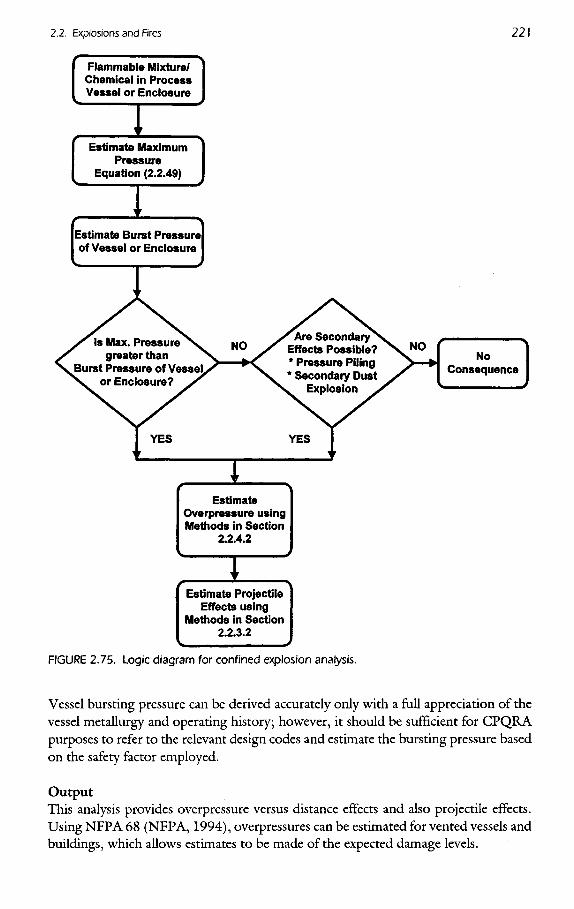
Logic DiagramThe logic of confined explosion modeling showing the stepwise procedure is providedin Figure 2.75.
Theoretical FoundationsAlthough the fundamentals of combustion and explosion theory have been evolvedover the last 100 years, the detailed application to most gases has been more recent. Forsimple molecules, the theoretical foundation is sound. For more complex species, par-ticularly dust and mists, the treatment is more empirical. Nevertheless, good experi-mental data have been pooled by the U.S. Bureau of Mines (Zabetakis, 1965; Kuchta,1973), NFPA 68 (NFPA, 1994), VDI3673 (VDI, 1995), andBartknecht (1989). Analternate approach is used in the UK and other parts of Europe as described bySchofield(1984).
Input Requirements and AvailabilityThe technology requires data on container strengths and combustion parameters. Thelatter are usually readily available; data on containment behavior are more difficult.
FIGURE 2.75. Logic diagram for confined explosion analysis.
Vessel bursting pressure can be derived accurately only with a full appreciation of thevessel metallurgy and operating history; however, it should be sufficient for CPQRApurposes to refer to the relevant design codes and estimate the bursting pressure basedon the safety factor employed.
OutputThis analysis provides overpressure versus distance effects and also projectile effects.Using NFPA 68 (NFPA51994), overpressures can be estimated for vented vessels andbuildings, which allows estimates to be made of the expected damage levels.
Flammable Mixture/Chemical in ProcessVessel or Enclosure
Estimate MaximumPressure
Equation (2.2.49)
Estimate Burst Pressureof Vessel or Enclosure
Is Max. Pressuregreater than
Burst Pressure of Vesselor Enclosure?
Are SecondaryEffects Possible?* Pressure Piling* Secondary Dust
Explosion
NoConsequence
EstimateOverpressure usingMethods in Section
2.2.4.2
Estimate ProjectileEffects using
Methods in Section2.2.3.2
Simplified ApproachesThe peak pressures achieved in confined explosions can be estimated as follows: defla-gration is eight times the initial absolute pressure, and detonation 20 times, for hydro-carbon-air mixtures. It can be assumed that pressure vessels fail at about four times thedesign working pressure. In the cases of dust explosions, the NFPA nomographs canbe used for relatively strong vessels and the modified Swift-Epstein equations indicatedin NFPA 68 (NFPA, 1994; see also Swift and Epstein, 1987) for low strength struc-tures (such as buildings).
2.2.5.3. EXAMPLE PROBLEM
Example 2.29: Overpressure from a Combustion in a Vessel. A im 3 vessel rated at1 barg contains a stoichiometric quantity of acetylene (C2H2) and air at atmosphericpressure and 250C. Estimate the energy released upon combustion and calculate thedistance at which a shock wave overpressure of 21 kPa can be obtained. Assume anenergy of combustion for acetylene of 301 kcal/gm-mole.
Solution: The stoichiometric combustion of acetylene at atmospheric pressureinside a vessel designed for 1 barg will produce pressures that will exceed the expectedburst pressure of the vessel.
The stoichiometric combustion of acetylene requires 2.5 mole of O2 per mole ofacetylene:
C2H2 + 2.5O2 -*• 2CO2 + H2O
1 mole of air contains 3.76 mole N2 and 1.0 mol O2. The starting composition isC2H2 + 2.5O2 + (2.5)(3.76)N2, resulting in the following initial gas mixture,
Compound Moles Mole fraction
C2H2 1.0 0.078
O2 2.5 0.194
N2 9.4 0.728
Total 12.9 1.000
A 1-m3 vessel at 250C contains
, /273KVl gm-mole^(Im3) — r =40.90gm- molev ;(298K^0.0224m3 j b
The amount of acetylene in this volume that could combust is
Since 1 kg of TNT is equivalent to 1120 kcal, then the TNT mass equivalent =960/1120 = 0.86 kg TNT. This represents the upper bound of the energy. The vessel
will probably begin to fail at about 5 barg. However, the rate of pressure rise during thecombustion may exceed the rate at which the vessel actually comes apart. The effectivefailure pressure, therefore, is somewhere between the pressure at which the vesselbegins to fail and the maximum pressure obtainable from combustion inside a closedvessel. As in physical explosions (Section 2.2.3) some fraction of the energy goes intoshock wave formation.
The most conservative assumption is to assume all of the combustion energy goesinto the shock wave. Thus, from Figure 2.48 for P5 = 21 kPa, Z = 7.83. Then from Eq.(2.2.7)
R^ =ZWl/* =(7.83m/kg1/3)(0.86kgTNT)1/3 =7.44m
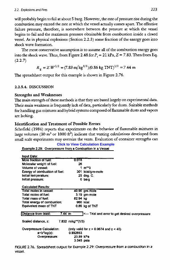
The spreadsheet output for this example is shown in Figure 2.76.
2.2.5.4. DISCUSSION
Strengths and WeaknessesThe main strength of these methods is that they are based largely on experimental data.Their main weakness is frequently lack of data, particularly for dusts. Suitable methodsfor handling gas mixtures and hybrid systems composed of flammable dusts and vaporsare lacking.
Identification and Treatment of Possible ErrorsSchofield (1984) reports that experiments on the behavior of flammable mixtures inlarge volumes (30 m3 or 1000 ft3) indicate that venting calculations developed fromsmall scale experiments may oversize the vents. Evaluation of container strengths can
Example 2.29: Overpressure from a Combustion in a Vessel
Input Data:Mole fraction of fuel: 0.078Molecular weight of fuel: 26Volume of vessel: 1 m**3Energy of combustion of fuel: 301 kcal/gm-moleInitial temperature: 25 deg. C.Initial pressure: O barg
Calculated Results:Total moles in vessel: 40.90 gm-moleTotal moles of fuel: 3.19 gm-moleTotal mass of fuel: 82.94 kgTotal energy of combustion: 960 kcalEquivalent mass of TNT 0.86 kg of TNT
!Distance from blast: 7.44 m ~|<— Trial and error to get desired overpressure
Scaled distance, z: 7.832 m/kg**(1/3)
Overpressure Calculation: (only valid for z > 0.0674 and z < 40)a+b*log(z): 0.992653Overpressure: 20.99 kPa
3.045 psia
FIGURE 2.76. Spreadsheet output for Example 2.29: Overpressure from a combustion in avessel.
be a main source of error. Vessels are often stronger than safety factors assume and thisfactor may be conservative in terms of the frequency or probability of vessel rupture,but conversely, not conservative in terms of calculating the consequences of rupture.
UtilityThe techniques discussed here are straightforward to apply and the data are readilyavailable (provided a simplistic estimate of bursting pressure is acceptable).
ResourcesA process engineer should be able to perform each type of calculation in an hour.
Available Computer CodesWin Vent (Pred Engineering, Inc., Palm City, FL)
2.2.6. Pool Fires
2.2.6.1. BACKGROUND
PurposePool fires tend to be localized in effect and are mainly of concern in establishing thepotential for domino effects and employee safety zones, rather than for communityrisk. The primary effects of such fires are due to thermal radiation from the flamesource. Issues of intertank and interplant spacing, thermal insulation, fire wall specifi-cation, etc., can be addressed on the basis of specific consequence analyses for a range ofpossible pool fire scenarios.
Drainage is an important consideration in the prevention of pool fires—if thematerial is drained to a safe location, a pool fire is not possible. See NFPA 30 (NFPA,1987a) for additional information. The important considerations are that (1) the liquidmust be drained to a safe area, (2) the liquid must be covered to minimize vaporization,(3) the drainage area must be far enough away from thermal radiation fire sources, (4)adequate fire protection must be provided, (5) consideration must be provided forcontainment and drainage of fire water and (6) leak detection must be provided.
PhilosophyPool fire modeling is well developed. Detailed reviews and suggested formulas are pro-vided in Bagster (1986), Considine (1984), Crocker and Napier (1986), Institute ofPetroleum (1987), Mudan (1984), Mudan and Croce (1988), and TNO (1979).
A pool fire may result via a number of scenarios. It begins typically with the releaseof flammable material from process equipment. If the material is liquid, stored at atemperature below its normal boiling point, the liquid will collect in a pool. The geom-etry of the pool is dictated by the surroundings (i.e., diking), but an unconstrained poolin an open, flat area is possible (see Section 2.1.2), particularly if the liquid quantityspilled is inadequate to completely fill the diked area. If the liquid is stored under pres-sure above its normal boiling point, then a fraction of the liquid will flash into vapor,with unflashed liquid remaining to form a pool in the vicinity of the release.
The analysis must also consider spill travel. Where can the liquid go and how farcan it travel?
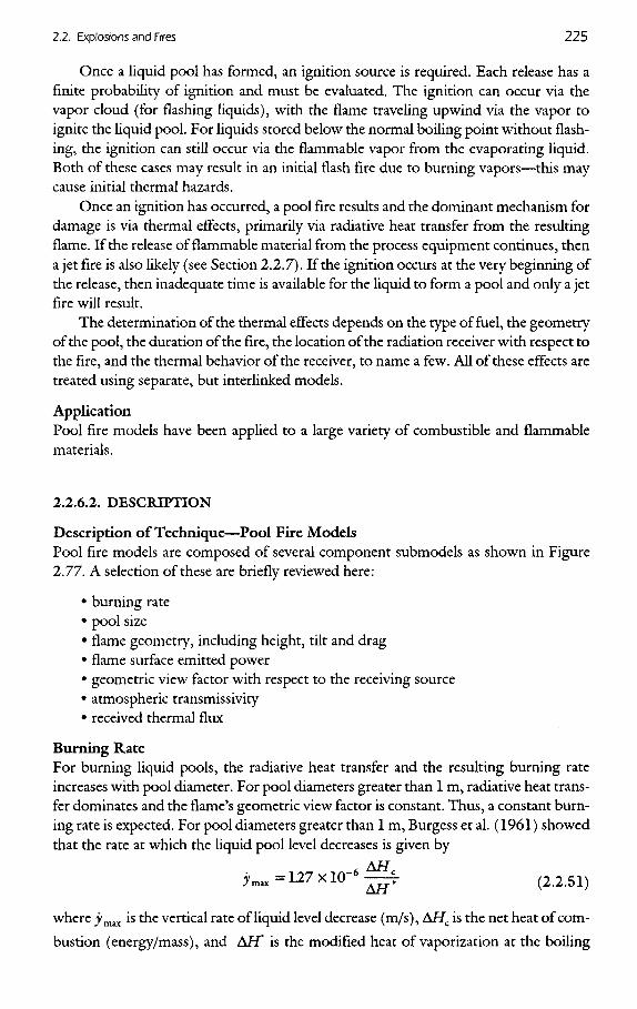
Once a liquid pool has formed, an ignition source is required. Each release has afinite probability of ignition and must be evaluated. The ignition can occur via thevapor cloud (for flashing liquids), with the flame traveling upwind via the vapor toignite the liquid pool. For liquids stored below the normal boiling point without flash-ing, the ignition can still occur via the flammable vapor from the evaporating liquid.Both of these cases may result in an initial flash fire due to burning vapors—this maycause initial thermal hazards.
Once an ignition has occurred, a pool fire results and the dominant mechanism fordamage is via thermal effects, primarily via radiative heat transfer from the resultingflame. If the release of flammable material from the process equipment continues, thena jet fire is also likely (see Section 2.2.7). If the ignition occurs at the very beginning ofthe release, then inadequate time is available for the liquid to form a pool and only a jetfire will result.
The determination of the thermal effects depends on the type of fuel, the geometryof the pool, the duration of the fire, the location of the radiation receiver with respect tothe fire, and the thermal behavior of the receiver, to name a few. All of these effects aretreated using separate, but interlinked models.
ApplicationPool fire models have been applied to a large variety of combustible and flammablematerials.
2.2.6.2. DESCRIPTION
Description of Technique—Pool Fire ModelsPool fire models are composed of several component submodels as shown in Figure2.77. A selection of these are briefly reviewed here:
• burning rate• pool size• flame geometry, including height, tilt and drag• flame surface emitted power• geometric view factor with respect to the receiving source• atmospheric transmissivity• received thermal flux
Burning RateFor burning liquid pools, the radiative heat transfer and the resulting burning rateincreases with pool diameter. For pool diameters greater than 1 m, radiative heat trans-fer dominates and the flame's geometric view factor is constant. Thus, a constant burn-ing rate is expected. For pool diameters greater than 1 m, Burgess et al. (1961) showedthat the rate at which the liquid pool level decreases is given by
ymax= 127 X 10-6^ (2.2.51)
where jymax is the vertical rate of liquid level decrease (m/s), AH0 is the net heat of com-
bustion (energy/mass), and AH* is the modified heat of vaporization at the boiling
FIGURE 2.77. Logic diagram for calculation of pool fire radiation effects.
point of the liquid given by Eq. (2.2.52) (energy/mass). Typical vertical rates are0.7 x IO"4 m/s (gasoline) to 2 X 1(T4
m/s (LPG).The modified heat of vaporization includes the heat of vaporization, plus an adjust-
ment for heating the liquid from the ambient temperature, Ta, to the boiling pointtemperature of the liquid, TBP.
AH*=AHV+£B P CpdT (2.2.52)
where A/fv is the heat of vaporization of the liquid at the ambient temperature(energy/mass) and Cp is the heat capacity of the liquid (energy/mass-deg).
Equation (2.2.52) can be modified for mixtures, or for liquids such as gasolinewhich are composed of a number of materials (Mudan and Croce, 1988).
The mass burning rate is determined by mutiplying the vertical burning rate by theliquid density. If density data are not available, the mass burning rate of the pool is esti-mated by
-a &Hm B = IX 1(T3-^- (2.2.53)
where mE is the mass burning rate (kg/m2 s).Equation (2.2.51) fits the experimental data better than Eq. (2.2.53), so the proce-
dure using the vertical burning rate and the liquid density is preferred. Typical valuesfor the mass burning rate for hydrocarbons are in the range of 0.05 kg/m2s (gasoline)to 0.12 kg/m2 s (LPG). Additional tabulations for the vertical and mass burning ratesare provided by Burgess and Zabetakis (1962), Lees (1986), Mudan and Croce (1988)and TNO (1979).
Equations (2.2.51) to (2.2.53) apply to liquid pool fires on land. For pool fires onwater, the equations are applicable if the burning liquid has a normal boiling point wellabove ambient temperature. For liquids with boiling points below ambient, heat trans-
Solid Plume RadiationModel
Estimate SurfaceEmitted Power
Equation (2.2.59)
Estimate GeometricView Factor
Equations (2.2.46),(2.2.47)
Estimate TrasmissivityEquation (2.2.42)
Estimate IncidentRadiation Flux
Equation (2.2.62)
Estimate RadiantFraction
Table 2.27
Estimate Point SourceLocation from Flame
Height
Estimate Point SourceView Factor
Equation (2.2.60)
(Estimate TransmissivityEquation (2.2.42)
Estimate IncidentRadiant Flux
Equation (2.2.61)
Point Source RadiationModel
FIGURE 2.77a. Logic diagram for the solidplume radiation model.
FIGURE 2.77b. Logic diagram for the pointsource radiation model.
fer between the liquid and the water will result in a burning rate nearly three times theburning rate on land (Mudan and Croce, 1988).
Pool SizeIn most cases, pool size is fixed by the size of the release and by local physical barriers(e.g., dikes, sloped drainage areas). For a continuous leak, on an infinite flat plane, themaximum diameter is reached when the product of burning rate and surface area equalsthe leakage rate.
D = 2 1 — (2.2.54)max \ny V ^
where Dmax is the equilibrium diameter of the pool (length), VL is the volumetric liquidspill rate (volume/time), and y is the liquid burning rate (length/time).
Equation (2.2.54) assumes that the burning rate is constant and that the dominantheat transfer is from the flame. More detailed pool burning geometry models are avail-able (Mudan and Croce, 1988).
Circular pools are normally assumed; where dikes lead to square or rectangularshapes, an equivalent diameter may be used. Special cases include spills of cryogenicliquids onto water (greater heat transfer) and instantaneous unbounded spills (Raj andKalelkar, 1974).
Flame HeightMany observations of pool fires show that there is an approximate ratio of flame heightto diameter. The best known correlation for this ratio is given by Thomas (1963) forcircular pool fires.
10.61
-^ (2.2.55)PaV^D
whereH is the visible flame height (m)D is the equivalent pool diameter (m)mE is the mass burning rate (kg/m2 s)pa is the air density (1.2 kg/m3 at 2O0C and 1 atm.)g is the acceleration of gravity (9.81 m/s2)Bagster (1986) summarizes rules of thumb forH/D ratios: Parker (1973) suggests
a value of 3 and Lees (1994) lists a value of 2.Moorhouse (1982) provides a correlation for the flame height based on large-scale
LNG tests. This correlation includes the effect of wind on the flame length:r -10.254
^=6.2 _^= M'-°-044 (2.2.56)D [p, VgD J 10
where U10* is a nondimensional wind speed determined using
*;°= K**JJ)/Pv r (2-2-57)
where uw is the measured wind speed at a 10m height (m/s) andpv is the vapor densityat the boiling point of the liquid (kg/m3).
Flame Tilt and DragPool fires are often tilted by the wind, and under stronger winds, the base of a pool firecan be dragged downwind. These effects alter the radiation received at surroundinglocations. A number of correlations have been published to describe these two factors.The correlation of Welker and Sliepcevich (1966) for flame tilt is frequently quoted,but the American Gas Association (AGA) (1974) andMudan (1984) note poor resultsfor LNG fires. The AGA paper proposes the following correlation for flame tilt:
cos 0 = 1 for u < 1
1 r . , (2.2.58)cosO=—= for u >1 '
Vu*
where u is the nondimensional wind speed given by Eq. (2.2.57) at a height of 1.6 mand 6 is the flame tilt angle (degrees or radians).
Flame drag occurs when wind pushes the base of the flame downwind from thepool, with the upwind edge of the flame and flame width remaining unchanged. Forsquare and rectangular fires the base dimension is increased in the direction of thewind. The thermal radiation downwind increases because the distance to a receiverdownwind is reduced. For circular flames, the flame shape changes from circular toelliptical, resulting in a change in view factor and a change in the radiative effects.Detailed flame drag correlations are provided by Mudan and Croce (1988).
Risk analyses can include or ignore tilt and drag effects. Flame tilt is more impor-tant; flame drag is an advanced topic, and many pool fire models do not include thiseffect. A vertical (untilted) pool fire is often assumed, as this radiates heat equally in alldirections. If a particularly vulnerable structure is located nearby and flame tilt couldaffect it, the CPQRA should consider tilt effects (both toward and away from the vul-nerable object) and combine these with appropriate frequencies allowing for the direc-tion of tilt.
Surface Emitted PowerThe surface emitted power or radiated heat flux may be computed from theStefan-Boltzmann equation. This is very sensitive to the assumed flame temperature,as radiation varies with temperature to the fourth power (Perry and Green, 1984). Fur-ther, the obscuring effect of smoke substantially reduces the total emitted radiationintegrated over the whole flame surface.
Two approaches are available for estimating the surface emitted power: the pointsource and solid plume radiation models. The point source is based on the total com-bustion energy release rate while the solid plume radiation model uses measured ther-mal fluxes from pool fires of various materials (compiled in TNO, 1979). Both thesemethods include smoke absorption of radiated energy (that process converts radiationinto convection). Typical measured surface emitted fluxes from pool fires are given byRaj (1977), Mudan (1984), and Considine (1984). LPG and LNG fires radiate up to250 kW/m2 (79,000 Btu/hr-ft2 ). Upper values for other hydrocarbon pool fires lie in
the range 110-170 kW/m2 (35,000-54,000 Btu/hr-ft2), but smoke obscuration oftenreduces this to 20-60 kW/m2 ( 6300-19,000 Btu/hr-ft2 ).
For the point source model, the surface emitted power per unit area is estimatedusing the radiation fraction method as follows:
1. Calculate total combustion power (based on burning rate and total pool area).2. Multiply by the radiation fraction to determine total power radiated.3. Determine flame surface area (commonly use only the cylinder side area).4. Divide radiated power by flame surface area.
The radiation fraction of total combustion power is often quoted in the range0.15-0.35 (Mudan, 1984; TNO, 1979). See Table 2.27.
While the point source model provides simplicity, the wide variability in the radia-tion fraction and the inability to predict it fundamentally detracts considerably fromthis approach.
The solid plume radiation model assumes that the entire visible volume of theflame emits thermal radiation and the nonvisible gases do not (Mudan and Croce,1988). The problem with this approach is that for large hydrocarbon fires, largeamounts of soot are generated, obscuring the radiating flame from the surroundings,and absorbing much of the radiation. Thus, as the diameter of the pool fire increases,the emitted flux decreases. Typical values for gasoline are 120 kW/m2 for a 1-m pool to20 kW/m2 for a 50-m diameter pool. To further complicate matters, the high turbu-lence of the flame causes the smoke layer to open up occasionally, exposing the hotflame and increasing the radiative flux emitted to the surroundings. Mudan and Croce(1988) suggest the following model for sooty pool fires of high molecular weighthydrocarbons to account for this effect,
E>v=Eme-SD+Es(I-e-SD) (2.2.59)where
£av is the average emissive power (kW/m2)Em is the maximum emissive power of the luminous spots (approximately
140 kW/m2)E5 is the emissive power of smoke (approximately 20 kW/m2)S is an experimental parameter (0.12 m"1)
D is the diameter of the pool (m)
TABLE 2.27. The Fraction of TotalEnergy Converted to Radiation forHydrocarbons (Mudan andCroce, 1988)
Fuel Fraction
Hydrogen 0.20
Methane 0.20
Ethylene 0.25
Propane 0.30
Butane 0.30
C5 and higher 0.40
Equation (2.2.59) produces an emissive power of 56 kW/m2 for a 10-m pool and20 kW/m2 for a 100-m pool. This matches experimental data for gasoline, kerosene andJP-4 fires reasonably well (Mudan and Croce, 1988).
Propane, ethane, LNG, and other low molecular weight materials do not produce
sooty flames.
Geometric View FactorThe view factor depends on whether the point source or solid plume radiation models
are used.For the point source model, the view factor is given by
PP=^ (2.2.60)
wherePp is the point source view factor (length"2) and* is the distance from the pointsource to the target (length).
Equation (2.2.60) assumes that all radiation arises from a single point and isreceived by an object perpendicular to this. This view factor must only be applied to thetotal heat output, not to the flux. Other view factors based on specific shapes (i.e., cyl-inders) require the use of thermal flux and are dimensionless. The point source viewfactor provides a reasonable estimate of received flux at distances far from the flame. Atcloser distances, more rigorous formulas or tables are given by Hamilton and Morgan(1952), Crocker and Napier (1986), and TNO (1979).
For the solid plume radiation model, the view factors^are provided in Figure 2.78for untilted flames and Figure 2.79 for tilted flames. Figure 2.78 requires an estimate ofthe flame height to diameter, while Figure 2.79 requires an estimate of the flame tilt.The complete equations for these figures are provided by Mudan and Croce (1988).Both figures provide view factors for a ground level receiver from a radiation source
Max
imum
Vie
w F
acto
r at G
roun
d Le
vel,
F 21
Dimensionless Distance from Flame Axis= Distance from Flame Axis / Pool Radius
FIGURE 2.78. Maximum view factors for a ground-level receptor from a right circular cylinder(Mudan and Croce, 1988).
Dlmensionless Distance from Flame Axis
= Distance from Flame Axis / Pool RadiusFIGURE 2.79. Maximum view factors for a ground-level receptor from a tilted circular cylinder(Mudan and Croce, 1988).
represented by a right circular cylinder. Note that near the source the view factor isalmost independent of the flame height since the observer is exposed to the maximumradiation.
Received Thermal FluxThe computation of the received thermal flux is dependent on the radiation modelselected.
If the point source model is selected, then the received thermal flux is determinedfrom the total energy rate from the combustion process:
Et = ̂ QrFf =r^ms^HcAFp (2.2.61)
If the solid plume radiation model is selected, the received flux is based on correla-tions of the surface emitted flux:
£r =raAHcf21 (2.2.62)
whereEr is the thermal flux received at the target (energy/area)ra is the atmospheric transmissivity, provided by Eq. (2.2.42) (unitless)Qx is the total energy rate from the combustion (energy/time)F is the point source view factor (length"2)
T] is the fraction of the combustion energy radiated, typically 0.15 to 0.35mE is the mass burning rate, provided by Eq. (2.2.53) (mass/area-time)
AHC is the heat of combustion for the burning liquid (energy/mass)A is the total area of the pool (length2)P21 is the solid plume view factor, provided by Eqs. (2.2.46) and (2.2.47)Values for the fraction of the combustion energy radiated, rj, are given in Table
2.27.
Max
imum
Vie
w F
acto
r at G
roun
d Le
vel,
F 21
Theoretical FoundationBurning rate, flame height, flame tilt, surface emissive power, and atmospherictransmissivity are all empirical, but well established, factors. The geometric view factoris soundly based in theory, but simpler equations or summary tables are oftenemployed. The Stefan-Boltzmann equation is frequently used to estimate the flamesurface flux and is soundly based in theory. However, it is not easily used, as the flametemperature is rarely known.
Input Requirements and AvailabilityThe pool size must be defined, either based on local containment systems or on somemodel for a flat surface. Burning rates can be obtained from tabulations or may be esti-mated from fuel physical properties. Surface emitted flux measurements are availablefor many common fuels or are calculated using empirical radiation fractions or solidflame radiation models. An estimate for atmospheric humidity is necessary fortransmissivity. All other parameters can be calculated.
OutputThe primary output of thermal radiation models is the received thermal radiation atvarious target locations. Fire durations should also be estimated as these affect thermaleffects (Section 2.3.2).
Simplified ApproachesCrocker and Napier (1986) provide tables of thermal impact zones from common situ-ations of tank roof and ground pool fires. From these tables, safe separation distancesfor people from pool fires can be estimated to be 3 to 5 pool diameters (based on a"safe" thermal impact of 4.7 kW/m2).
2.2.6.3. EXAMPLE PROBLEM
Example 2.30: Radiation from a Burning Pool. A high molecular weight hydrocar-bon liquid escapes from a pipe leak at a volumetric rate of 0.1 m3/s. A circular dike witha 25 m diameter contains the leak. If the liquid catches on fire, estimate the thermal fluxat a receiver 50 m away from the edge of the diked area. Assume a windless day with50% relative humidity. Estimate the thermal flux using the point source and the solidplume radiation models.
Additional Data:Heat of combustion of the liquid: 43,700 kj/kgHeat of vaporization of the liquid: 300 kj/kgBoiling point of the liquid: 363 KAmbient temperature: 298 KLiquid density: 730 kg/m3
Heat capacity of liquid (constant): 2.5 kJ/kg-K
Solution: Since the fuel is a high molecular weight material, a sooty flame isexpected. Equations (2.2.51) and (2.2.53) are used to determine the vertical burning
rates and the mass burning rates, respectively. These equations require the modifiedheat of vaporization, which can be calculated using Eq. (2.2.52):
The mass burning rate is determined by multiplying the vertical burning rate bythe density of the liquid:
^B =P>max = (730 kg/m3)(1.20 XlO"4 m/s) =0.0876 kg/m2 s
The maximum, steady state pool diameter is given by Eq. (2.2.54),
fr>T I (0.10 m3/s)Anax =2,-^- =2J '—. =32.6 m
\*y V (3.14)(1.20x KT4 m/s)
Since this is larger than the diameter of the diked area, the pool will be constrainedby the dike with a diameter of 25 m. The area of the pool is
,J-JgI-'"4"*-"'-491m'4 4
The flame height is given by Eq. (2.2.55),
n*i r ~i°-61
H ( mn } (0.0876 kg/m2 s)— = 42 ^= =42 i , 6/ ; = =1.59D IPaVSDj [(1.2 kg/m3)7(9.81 m/s2)(25 m)
Thus, H= (1.59)(25m) = 39.7m
Point Source Model. This approach is based on representing the total heat release asa point source. The received thermal flux for the point source model is given by Eq.(2.2.61). The calculation requires values for the atmospheric transmissivity and theview factor. The view factor is given by Eq. (2.2.60), based on the geometry shown inFigure 2.80. The point source is located at the center of the pool, at a height equal tohalf the height of the flame. This height is (39.7 m)/2 = 19.9 m. From the right trian-gle formed,
x2 = (19.9 m)2 + (25 + 50 m)2 = 6020 m2
x = 77.6 m
This represents the beam length from the point source to the receiver. The viewfactor is determined using Eq. (2.2.60)
Figure 2.78 is used to determine the geometric view factor. This requires theheight to pool radius ratio and the dimensionless distance. Since H/D = 1.59, H/R =2(1.59) = 3.18. The dimensionless distance to the receiver is X/R, where R is theradius of the pool and X is the distance from the flame axis to the receiver, that is,50 m + 25/2 m = 62.5 m. Thus, ̂ R = 62.5 m/12.5 m = 5 and from Figure 2.78,F21 = 0.068.
The atmospheric transmissivity is given by Eq. (2.2.42)
ra =2.02(PwXs)"a°9 =(2.02) [(158O Pa) (SOm)]-0-09 =0.732
The radiant flux at the receiver is determined from Eq. (2.2.45)
Er =r a AHCP21 =(0.732)(26.0kW/m2)(0.068)=1.3kJ/m2s = 1.3kW/m2
The result from the solid plume radiation model is smaller than the point sourcemodel. This is most likely due to consideration of the radiation obscuration by the
Fire
Receptor
Pool
flame soot, a feature not treated directly by the point source model. The differencesbetween the two models might be greater at closer distance to the pool fire.
The spreadsheet output for this example is shown in Figure 2.81.
Example 2.30: Radiation from a Burning Pool
Input Data:Tfquid leakage rate: 0.1 m**3/sHeat of combustion of liquid: 43700 kJ/kgHeat of vaporization of liquid: 300 kJ/kgBoiling point of liquid: 363 KAmbient temperature: 298 KLiquid density: 730 kg/m**3Constant heat capacity of liquid: 2.5 kJ/kg-KDike diameter: 25 mReceptor distance from pool: 50 mRelative humidity: 50 %Radiation efficiency for point source mode 0.35
Calculated Results:Modified heat of vaporization: 462.5 kJ/kgVertical burning rate: 1.20E-04 m/sMass burning rate: 0.087598 kg/m**2-sMaximum pool diameter: 32.57 mDiameter used in calculation: 25 mArea of pool: 490.87 m**2Flame H/D: 1.59Flame height: 39.72 mPartial pressure of water vapor: 1579.95 Pa
Point Source Model:Point source height: 19.86mDistance to receptor: 77.58 mView factor: 1.3E-05 m**(-2)Transmissivity: 0.70!Thermal flux at receptor. 6.12 kW/m**2 |
Solid Plume Radiation Model:Source emissive power: 25.97Distance from flame axis to receptor: 62.5Flame radius: 12.5Flame H/R ratio: 3.18Dimensionless distance from flame axis: 5.00
Strengths and WeaknessesPool fires have been studied for many years and the empirical equations used in thesubmodels are well validated. The treatment of smoky flames is still difficult. A weak-ness with the pool models is that flame impingement effects are not considered; theygive substantially higher heat fluxes than predicted by thermal radiation models.
Identification and Treatment of Possible ErrorsThe largest potential error in pool fire modeling is introduced by the estimate for sur-face emitted flux. Where predictive formulas are used (especially Stefan-Boltzmanntypes) simple checks on ratios of radiated energy to overall combustion energy shouldbe carried out. Pool size estimates are important, and the potential for dikes or othercontainment to be overtopped by fluid momentum effects or by foaming should beconsidered.
UtilityPool fire models are relatively straightforward to use.
Resources NecessaryA trained process engineer will require several hours to complete a pool fire scenario byhand if all necessary thermodynamic data, view factor formulas, and humidity data areavailable.
Available Computer CodesDAMAGE (TNO, Apeldoorn, The Netherlands)PHAST (DNV, Houston, TX)QRAWorks (PrimaTech, Columbus, OH)TRACE (Safer Systems, Westlake Village, CA)SUPERCHEMS (Arthur D. Little, Cambridge, MA)
2.2.7. Jet Fires
2.2.7.1. BACKGROUND
PurposeJet fires typically result from the combustion of a material as it is being released from apressurized process unit. The main concern, similar to pool fires, is in local radiationeffects.
ApplicationThe most common application of jet fire models is the specification of exclusion zonesaround flares.
2.2.7.2. DESCRIPTION
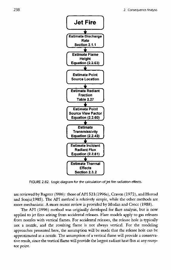
Description of TechniqueJet fire modeling is not as well developed as for pool fires, but several reviews have beenpublished. Jet fire modeling incorporates many mechanisms, similar to those consid-ered for pool fires, as is shown on the logic diagram in Figure 2.82. Three approaches
FIGURE 2.82. Logic diagram for the calculation of jet fire radiation effects.
are reviewed by Bagster (1986): those of API 521(1996a), Craven (1972), andHustadand Sonju(1985). The API method is relatively simple, while the other methods aremore mechanistic. A more recent review is provided by Mudan and Croce (1988).
The API (1996) method was originally developed for flare analysis, but is nowapplied to jet fires arising from accidental releases. Flare models apply to gas releasesfrom nozzles with vertical flames. For accidental releases, the release hole is typicallynot a nozzle, and the resulting flame is not always vertical. For the modelingapproaches presented here, the assumption will be made that the release hole can beapproximated as a nozzle. The assumption of a vertical flame will provide a conserva-tive result, since the vertical flame will provide the largest radiant heat flux at any recep-tor point.
Jet Fire
Estimate DischargeRate
Section 2.1.1
Estimate FlameHeight
Equation (2.2.63)
Estimate PointSource Location
Estimate RadiantFraction
Table 2.27
Estimate PointSource View Factor
Equation (2.2.60)
EstimateTransmissivity
Equation (2.2.42)
Estimate IncidentRadiant Flux
Equation (2.2.61)
Estimate ThermalEffects
Section 2.3.2
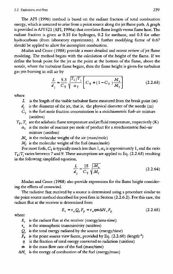
The API (1996) method is based on the radiant fraction of total combustionenergy, which is assumed to arise from a point source along the jet flame path. A graphis provided in API 521 (API, 1996a) that correlates flame length versus flame heat. Theradiant fraction is given as 0.15 for hydrogen, 0.2 for methane, and 0.3 for otherhydrocarbons (from laboratory experiments). A further modifying factor of 0.67should be applied to allow for incomplete combustion.
Mudan and Croce (1988) provide a more detailed and recent review of jet flamemodeling. The method begins with the calculation of the height of the flame. If wedefine the break point for the jet as the point at the bottom of the flame, above thenozzle, where the turbulent flame begins, then the flame height is given for turbulentgas jets burning in still air by
L 5'3 |Tf/ri L , n r x^.l n->M\— = — — cT+(1-C7)- (2.2.63)A.} C7 y «T L Mf ]
whereL is the length of the visible turbulent flame measured from the break point (m)
A- is the diameter of the jet, that is, the physical diameter of the nozzle (m)C7 is the fuel mole fraction concentration in a stoichiometric fuel-air mixture
(unitless)Tp, TJ are the adiabatic flame temperature and jet fluid temperature, respectively (K)
aT is the moles of reactant per mole of product for a stoichiometric fuel-airmixture (unitless)
Ma is the molecular weight of the air (mass/mole)Mf is the molecular weight of the fuel (mass/mole)For most fuels, C7 is typically much less than 1, aT is approximately 1, and the ratio
Tp/Ty varies between 7 and 9. These assumptions are applied to Eq. (2.2.63) resultingin the following simplified equation,
L 15 [M~T^\W( <2-2-64>
Mudan and Croce (1988) also provide expressions for the flame height consider-ing the effects of crosswind.
The radiative flux received by a source is determined using a procedure similar tothe point source method described for pool fires in Section (2.2.6.2). For this case, theradiant flux at the receiver is determined from
E1 = r1QIFp =r,r,mAHcFf (2.2.65)where
Er is the radiant flux at the receiver (energy/area-time)ra is the atmospheric transmissivity (unitless)Q1. is the total energy radiated by the source (energy/time)Fp is the point source view factor, provided by Eq. (2.2.60) (length"2)
rj is the fraction of total energy converted to radiation (unitless)m is the mass flow rate of the fuel (mass/time)
AH0 is the energy of combustion of the fuel (energy/mass)
For this model, the point source is located at the center of the flame, that is, halfwayalong the flame centerline from the break point to the tip of the flame, as determined byEqs. (2.2.63) or (2.2.64). It is assumed that the distance from the nozzle to the breakpoint is negligible with respect to the total flame height. The fraction of the energy con-verted to radiative energy is estimated using the values provided in Table 2.27.
None of the above methods consider flame impingement. In assessing the poten-tial for domino effects on adjacent hazardous vessels, the dimensions of the jet flamecan be used to determine whether flame impingement is likely. If so, heat transfereffects will exceed the radiative fraction noted above, and a higher heat fraction couldbe transferred to the impinged vessel.
Theoretical FoundationsThe models to predict the jet flame height are empirical, but well accepted and docu-mented in the literature. The point source radiation model only applies to a receiver at adistance from the source. The models only describe jet flames produced by flammablegases in quiescent air—jet flames produced by flammable liquids or two-phase flowscannot be treated. The empirically based radiant energy fraction is also a source of error.
Input RequirementsThe jet flame models require an estimate of the flame height, which is determined froman empirical equation based on reaction stoichiometry and molecular weights. Thepoint source radiant flux model requires an estimate of the total energy generation ratewhich is determined from the mass flow rate of combustible material. The fraction ofenergy converted to radiant energy is determined empirically based on limited experi-mental data. The view factors and atmospheric transmissivity are determined usingpublished correlations.
Simplified ApproachesConsidine and Grint (1984) give a simplified power law correlation for LPG jet firehazard zones. The dimensions of the torch flame, which is assumed to be conical, aregiven by
L = 9.1m05 (2.2.66)
W=0.25L (2.2.67)
rs>50 = 1.9t°AmQA7 (2.2.68)
whereL is the length of torch flame (m)W is the jet flame conical half-width at flame tip (m)m is the LPG release rate subject to 1 < m < 3000 kg/s (kg/s)rs 50 is the side-on hazard range to 50% lethality, subject to r > W (m)
t is the exposure time, subject to 10 < t < 300 s (s)
2.2.7.3. EXAMPLE PROBLEM
Example 2.31: Radiant Flux from a Jet Fire. A 25-mm hole occurs in a large pipe-line resulting in a leak of pure methane gas and a flame. The methane is at a pressure of
100 bar gauge. The leak occurs 2-m off the ground. Determine the radiant heat flux at apoint on the ground 15 m from the resulting flame. The ambient temperature is 298 Kand the humidity is 50% RH.
Additional Data:Heat capacity ratio, £, for methane: 1.32Heat of combustion for methane: 50,000 kj/kgFlame temperature for methane: 2200 K
Solution: Assume a vertical flame for a conservative result and that the release holeis represented by a nozzle. The height of the flame is calculated first to determine thelocation of the point source radiator. This is computed using Eq. (2.2.63)
_ L _ _ 5 3 F±B\C + l_c }M74. ~CT ^l «T [ T ( TX_
The combustion reaction in air is
CH4 + 2O2 + 7.52N2 -* CO2 + 2H2O + 7.52N2
Thus, Cx = 1/(1 + 2 + 7.52) = 0.095, Tf/T- = 2200/298 = 7.4 andaT = 1.0. Themolecular weight of air is 29 and for methane 16. Substituting into Eq. (2.2.63),
^^jissh95^-0-095'!]=200
Note that Eq. (2.2.64) yields a value of 212, which is close to the value of 200 pro-duced using the more detailed approach. Since the diameter of the issuing jet is 25 mm,the flame length is (200)(25 mm) = 5.00 m.
Figure 2.83 shows the geometry of the jet flame. Since the flame base is 2 m off theground, the point source of radiation is located at 2 m + (5.00 m)/2 = 4.50 m abovethe ground.
The discharge rate of the methane is determined using Eq. (2.1.17) for chokedflow of gas through a hole. For this case,
Jet Flame
Receptor
FIGURE 2.83. Geometry for Example 2.31: Radiant flux from a jet fire.
(for choked flow through a hole)
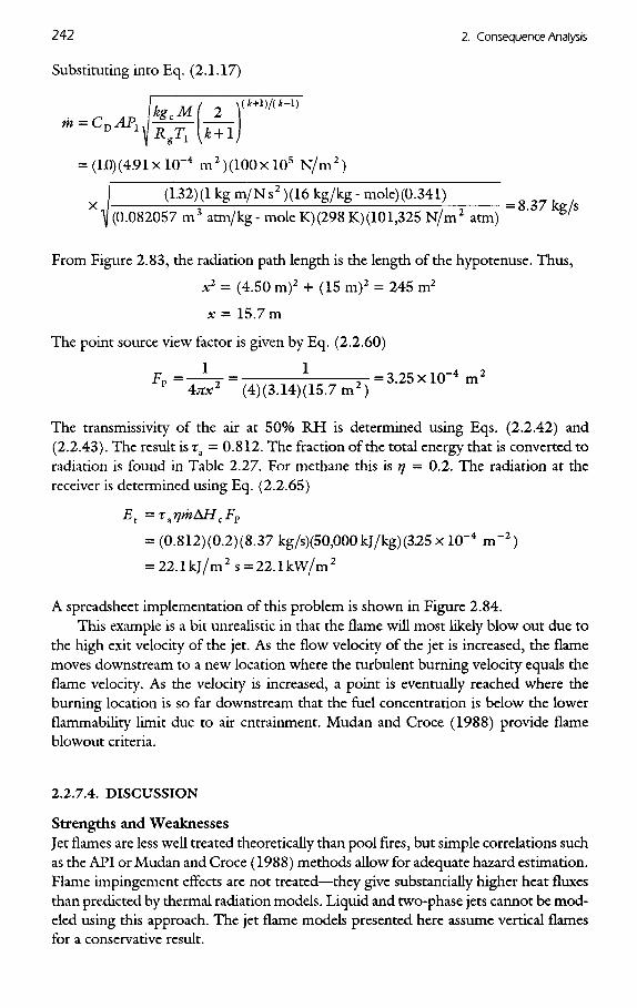
Substituting into Eq. (2.1.17)
Ike M( 2 V4+W*-1'
*-c»^ J^lifiJ= (1.0)(4.91 XlO'4 m2)(100XlO5 N/m2)
x I (132X1 kg °VNs2)(16 kg/kg - mole)(0.341)1J (0.082057 m3 atm/kg - mole K)(298 K)(101,325 N/m2 atm) ' S/§
From Figure 2.83, the radiation path length is the length of the hypotenuse. Thus,
x2 = (4.50 m)2 + (15 m)2 = 245 m2
x = 15.7 m
The point source view factor is given by Eq. (2.2.60)
Fp=4^r = (4)(3.14)(15.7m2)=3-25Xl°"4m2
The transmissivity of the air at 50% RH is determined using Eqs. (2.2.42) and(2.2.43). The result is ra = 0.812. The fraction of the total energy that is converted toradiation is found in Table 2.27. For methane this is r\ = 0.2. The radiation at thereceiver is determined using Eq. (2.2.65)
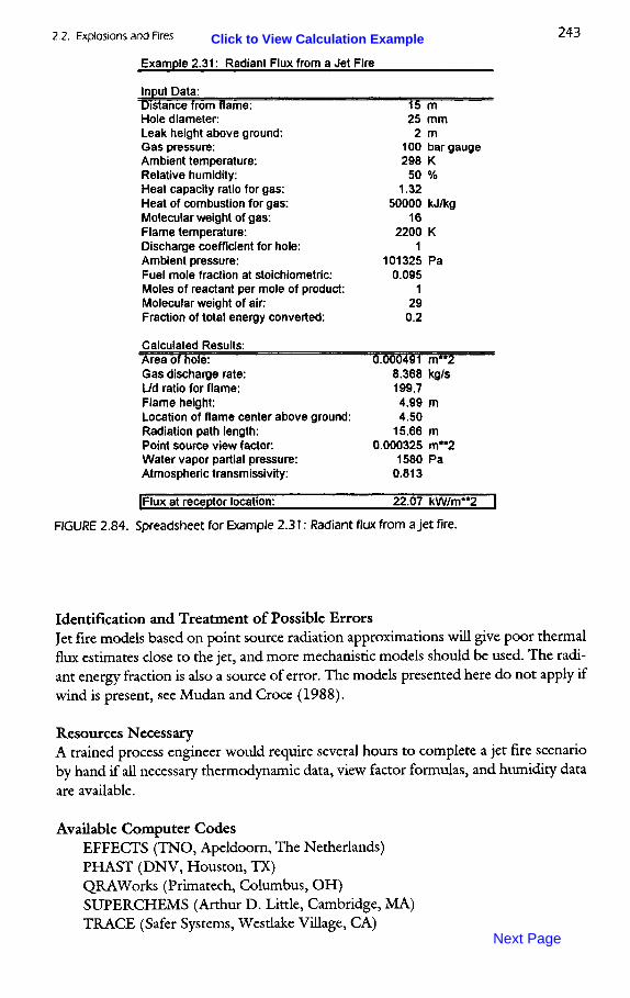
A spreadsheet implementation of this problem is shown in Figure 2.84.This example is a bit unrealistic in that the flame will most likely blow out due to
the high exit velocity of the jet. As the flow velocity of the jet is increased, the flamemoves downstream to a new location where the turbulent burning velocity equals theflame velocity. As the velocity is increased, a point is eventually reached where theburning location is so far downstream that the fuel concentration is below the lowerflammability limit due to air entrainment. Mudan and Croce (1988) provide flameblowout criteria.
2.2.7.4. DISCUSSION
Strengths and WeaknessesJet flames are less well treated theoretically than pool fires, but simple correlations suchas the API or Mudan and Croce (1988) methods allow for adequate hazard estimation.Flame impingement effects are not treated—they give substantially higher heat fluxesthan predicted by thermal radiation models. Liquid and two-phase jets cannot be mod-eled using this approach. The jet flame models presented here assume vertical flamesfor a conservative result.
Example 2.31: Radiant Flux from a Jet Fire
Input Data:Distance from flame: 1 5 mHole diameter: 25 mmLeak height above ground: 2 mGas pressure: 100 bar gaugeAmbient temperature: 298 KRelative humidity: 50 %Heat capacity ratio for gas: 1.32Heat of combustion for gas: 50000 kJ/kgMolecular weight of gas: 16Flame temperature: 2200 KDischarge coefficient for hole: 1Ambient pressure: 101325 PaFuel mole fraction at stoichiometric: 0.095Moles of reactant per mole of product: 1Molecular weight of air: 29Fraction of total energy converted: 0.2
Calculated Results:Area of hole: 0.000491 m**2Gas discharge rate: 8.368 kg/sUd ratio for flame: 199.7Flame height: 4.99 mLocation of flame center above ground: 4.50Radiation path length: 15.66 mPoint source view factor: 0.000325 m**2Water vapor partial pressure: 1580 PaAtmospheric transmissivity: 0.813
[Flux at receptor location: 22.07 kW/m**2 |
FIGURE 2.84. Spreadsheet for Example 2.31: Radiant flux from a jet fire.
Identification and Treatment of Possible ErrorsJet fire models based on point source radiation approximations will give poor thermalflux estimates close to the jet, and more mechanistic models should be used. The radi-ant energy fraction is also a source of error. The models presented here do not apply ifwind is present, see Mudan and Croce (1988).
Resources NecessaryA trained process engineer would require several hours to complete a jet fire scenarioby hand if all necessary thermodynamic data, view factor formulas, and humidity dataare available.
Available Computer CodesEFFECTS (TNO, Apeldoorn, The Netherlands)PHAST (DNV, Houston, TX)QRAWorks (Primatech, Columbus, OH)SUPERCHEMS (Arthur D. Little, Cambridge, MA)TRACE (Safer Systems, Westlake Village, CA)