Eleanor KrauseRichard V. ReevesSeptember 2017

Rural dreams: Upward mobility in America's countryside

2RURAL DREAMS: UPWARD MOBILITY IN AMERICA'S COUNTRYSIDE

Executive SummaryOne of the defining features of the “American Dream” is the ability to succeed despite being born in disadvantaged circumstances. But upward mobility, in the sense of doing better than your parents, appears to be on the wane. There is however a great deal of variation across the nation in rates of upward mobility, and some of the greatest variation lies in the nation’s rural heartland. While some rural counties exhibit the nation’s lowest rates of upward mobility, others can still lay claim to being “lands of opportunity,” ensuring that young residents are prepared to take on adulthood and work their way up the socioeconomic ladder. Why is the American Dream still alive and well in some areas, but not others? What factors are most associated with upward mobility in these rural communities?

To answer these questions, in this paper we merge county-level socioeconomic data with mobility datasets from the Equality of Opportunity Project, a research project led by Raj Chetty, John Friedman, and Nathaniel Hendren. These scholars and their team have pioneered modern mobility research, which is a growing field of scholarship. But so far, little attention has been paid upward mobility in rural communities.

We consider the factors associated with upward mobility in counties that are only home to about 4 percent of the nation’s population, living in the most economically isolated and sparsely populated counties in the country. These rural residents often face unique barriers to opportunity compared to their urban counterparts, who can more readily take advantage of the economic activity, educational opportunities, and diversity of metropolitan areas. So, what explains the dramatic variation in upward mobility in America’s rural areas?

• Our own analysis confirms the findings of Chetty et al. (2014) that high-mobility areas have higher quality K-12 education, improved measures of family stability, greater social capital, lower income inequality, and less residential segregation. When we restrict our analysis to only the most rural counties, these relationships remain strong, though proxies for segregation and inequality appear less correlated with upward mobility in rural counties than in all counties. • One of the most striking differences between high- and low-mobility rural counties is the rate of net migration. Counties with the highest rates of absolute mobility also have the most negative rates of net migration in the 2000-2010 period, particularly among those ages 15-24. The mobility statistics are anchored to where the individual lived at age 16, so these counties appear to be providing young residents with some beneficial combination of factors that improve their outcomes later on.• Some of the most influential factors considered by Chetty et al. (2014) appear more associated with upward mobility in rural counties. Variables such as school expenditures per student, student-teacher ratios, the fraction of children with single mothers, and teen birth rates were highly associated with upward mobility in rural counties. The teen birth rate in the lowest-

3 CENTER ON CHILDREN AND FAMILIES AT BROOKINGSKRAUSE, REEVES

performing quartile of rural counties was nearly twice that of the highest-mobility rural counties.• Unsurprisingly, the strength of the local economy is also associated with upward mobility. Rural counties with the highest rates of upward mobility also had higher labor force participation rates and lower poverty rates than those with very low rates of upward mobility. Of particular note was the difference between teen labor force participation rates – the highest-performing quartile of rural counties had an average teen labor force participation rate of 64 percent, compared to 35 percent in the lowest-performing group. This is likely a sign of a stronger local economy, but also suggests that teens in these high-mobility counties are gaining valuable work experience in their early years that might benefit their labor market opportunities down the road.

What do these findings mean for policymakers? A sweeping set of policy prescription for rural America is beyond the scope of this paper. But there are three arenas that seem particularly promising for bolstering opportunity in rural America. First, invest in human capital development; improving K-12 quality in distressed areas will improve young residents’ preparedness for adulthood and life prospects. Second, ensure that these communities are equipped with basic 21st century infrastructure, like broadband, that will enable them to better connect to distant economies and opportunities. Finally, invest in family planning. Rural residents are less likely to have access to affordable and quality health care, which makes intentional parenthood more difficult.

So: upward mobility is being realized in some rural counties. Moving away to places with greater opportunities is part of the story; but it is not the whole one. Investing in skills, stability and connectedness can fuel upward mobility both for those who leave and those who choose to stay.

4RURAL DREAMS: UPWARD MOBILITY IN AMERICA'S COUNTRYSIDE

The American Dream in America’s heartland The opportunity to rise up the income ladder – from “rags to riches” – is a quintessential element of the American Dream. But there are huge differences in the odds of upward mobility between different parts of the U.S., as work by Raj Chetty and colleagues has shown. Growing up to be better off than one’s parents – upward “absolute intergenerational mobility” – looks to be far more difficult in some corners of this country than others. Some communities have proven successful at providing economic opportunity to children across the income spectrum. Others appear to be “mobility traps,” where children born to disadvantaged circumstances are extremely unlikely to get ahead. Most of the research on geographical variations in mobility has focused on cities. This is understandable: after all, 85 percent of the population lives in counties designated as metropolitan. The danger, however, is that those who live in rural areas receive less attention from policymakers. In this paper, we analyze intergenerational mobility rates in nearly 750 of the most rural counties in the United States. Even though these counties account for a fairly small slice of the population, around 4 percent, they face specific and in many cases deepening challenges. By many measures, rural residents appear to be worse-off than urban ones, with lower incomes, lower levels of educational attainment, lower life expectancies, and limited access to health insurance and health care providers. Rural areas are, by definition, often relatively isolated from the economic activity, educational opportunities, and labor market diversity of urban metropolises, so rural residents may face different obstacles to upward mobility than their urban counterparts. Many are dominated by a single industry and are thus more exposed to labor market shocks than more diversified economies. Rural counties are more likely to be persistently poor, with at least a 20 percent poverty rate persisting for at least 30 years. As Janet Adamy and Paul Overberg report in the Wall Street Journal, “In terms of poverty, college attainment, teenage births, divorce, death rates from heart disease and cancer, reliance on federal disability insurance and male labor-force participation, rural counties now rank the worst.”

Urban counties witnessed steady population gains over the 21st century, while 2010-2016 marked the first period in which non-metro counties as a whole witnessed net population decline. This is owing, in part, to out-migration. But it also reflects the recent, startling increase in mid-life mortality rates among white men and women that has occurred alongside declining health and an opioid epidemic in rural and small-town America. Premature death rates are consistently higher in rural counties than in urban ones. Anne Case and Angus Deaton labelled the collective influence of drug overdoses, alcohol poisonings, and suicides “deaths of despair,” and they hypothesize that the recent uptick in these deaths of despair among the white working class might be attributable to

5 CENTER ON CHILDREN AND FAMILIES AT BROOKINGSKRAUSE, REEVES

declining labor market prospects and other economic factors.

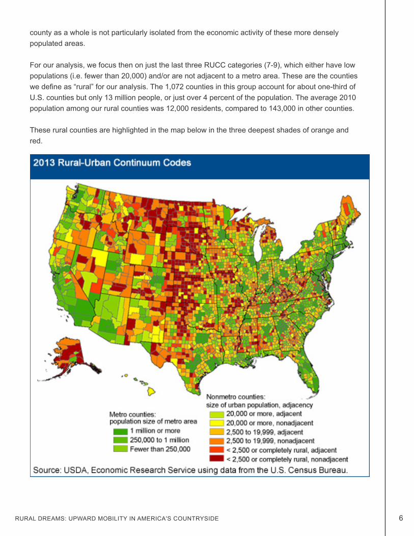
What counts as rural? Before assessing mobility rates in rural counties, we have to decide what counts as “rural.” This is not a straightforward question: different agencies use slightly different criteria for defining “rural.” The U.S. Census Bureau defines rural as essentially any place that is not urban or “metropolitan.” In this paper, we use the U.S. Department of Agriculture Economic Research Service’s Rural-Urban Continuum Codes (RUCC). Every county in America is classified in the RUUC as either “metro” or “non-metro,” but within these categories lies extensive variation. The RUCC classification consists of three metro and six non-metro categories:

In total, as of July 2015, non-metro counties represented about two-thirds of all counties, 14 percent of the population, and 72 percent of the nation’s land area. But many of these counties are adjacent to a metro area, and with reasonably large populations. Take Franklin County, Kentucky for example, with a population of about 49 thousand and home to that state capital, Frankfort. Residents can drive to either Louisville or Lexington in about an hour. While some residents of Franklin County certainly live in the outskirts of town and would consider themselves “rural,” the

2013 Rural-Urban Continuum CodesNumber of counties in sample

Avg. population in 2010

Counties in metro areas of 1 million population or more

Counties in metro areas of 250,000 to 1 million population

Counties in metro areas of fewer than 250,000 population

431

379

356

Description 2010 population

390,877

173,113

79,546

168,468,073

65,609,941

28,318,216

Code

1.

2.

3.

Metro counties 1,166 225,040 262,396,290

Non-metro counties 1,976 23,480 46,395,946

Urban population of 20,000 or more, adjacent to a metro area

Urban population of 20,000 or more, not adjacent to a metro area

Urban population of 2,500 to 19,999, adjacent to a metro area

Urban population of 2,5000 to 19,999, not adjacent to a metro area

Completely rural or less than 2,500 urban population, adjacent to a metro area

Completely rural or less than 2,500 urban population, not adjacent to a metro area

4.

5.

6.

7.

8.

9.

214

92

593

433

220

419

63,263

53,846

24,933

19,050

9,807

6,194

13,538,323

4,953,810

14,784,978

8,248,676

2,157,448

2,595,315

U.S. total 3,137 98,398 308,674,777

6RURAL DREAMS: UPWARD MOBILITY IN AMERICA'S COUNTRYSIDE

county as a whole is not particularly isolated from the economic activity of these more densely populated areas.

For our analysis, we focus then on just the last three RUCC categories (7-9), which either have low populations (i.e. fewer than 20,000) and/or are not adjacent to a metro area. These are the counties we define as “rural” for our analysis. The 1,072 counties in this group account for about one-third of U.S. counties but only 13 million people, or just over 4 percent of the population. The average 2010 population among our rural counties was 12,000 residents, compared to 143,000 in other counties.

These rural counties are highlighted in the map below in the three deepest shades of orange and red.

7 CENTER ON CHILDREN AND FAMILIES AT BROOKINGSKRAUSE, REEVES

Measuring upward mobility in the rural heartland: our approach In “Where is the Land of Opportunity? The Geography of Intergenerational Mobility in the United States,” Raj Chetty, Nathaniel Hendren, Patrick Kline, and Emmanuel Saez examine the factors most strongly associated with upward mobility in America’s largest commuting zones (CZs). Chetty et al. (2014) summarize their results as showing that “the spatial differences in mobility are driven by factors that affect children while they are growing up rather than after they enter labor market” (p. 3).

We use county-level estimates of upward mobility generated by Chetty and his colleagues at the Equality of Opportunity Project to extend the researchers’ original analysis to consider mobility in America’s most rural counties. Their estimates are available for 741 of these 1,072 rural counties. Missing counties are primarily the result of very small populations, from which mobility statistics could not be calculated. Specifically, we use the author’s preferred estimate for absolute upward mobility: the expected mean income rank of children (in the national child income distribution) with parents at the 25th percentile of the national parent income distribution.1 Parental income is the average parents’ pre-tax family income at the household level over the five years from 1996 to 2000 (when the child is around 16 years old); children’s adult income was measured when they were in their early 30’s in 2011 and 2012, and compared to their parents’ incomes at the same age. So a person who grows up in Nashville, Tennessee until the age of 18, attends college at the University of Tennessee in Knoxville, and goes on to work in Durham, North Carolina would be considered in the mobility statistics for Nashville.

We also examine a series of county-level independent social and economic variables. Many of these (e.g. school expenditures per student, labor force participation rate, etc.) were also retrieved from the Equality of Opportunity Project – in this case from Chetty and Hendren (2017). The full list of independent variables and their relationship with absolute mobility is in the Appendix.2

In addition to the independent variables retrieved from Chetty and Hendren (2017), we include in our analysis two measures of net migration – the balance of in-migrants minus out-migrants – over the 2000-2010 decade from Winkler et al. (2013).3 The first measure is for net migration across all age groups; the second is for 15-24 year olds.

Correlates for these variables were determined with absolute upward mobility as the dependent

1 Chetty et al. (2014) find a nearly linear relationship between mean child and parent ranks within commuting zones. Thus, they summarize the conditional expectation of a child’s rank given a parent’s rank using the slope and intercept from a regression of child rank and parent rank. They term “absolute upward mobility” the “mean rank (in the national child income distribution) of children whose parents are at the 25th percentile of the national parent income distribution.” They contend that when this statistic is tied to relatively small areas in the U.S. (i.e. a county), “a child’s rank in the national income distribution is effectively an absolute outcome because incomes in a given area have little impact on the national distribution” (p. 7).2 More detailed variable descriptions and sources can also be found in Chetty and Hendren (2017) “Online appendix table XV.”3 Winkler et al. (2013) developed these estimates from U.S. Census counts and birth and death records.

8RURAL DREAMS: UPWARD MOBILITY IN AMERICA'S COUNTRYSIDE

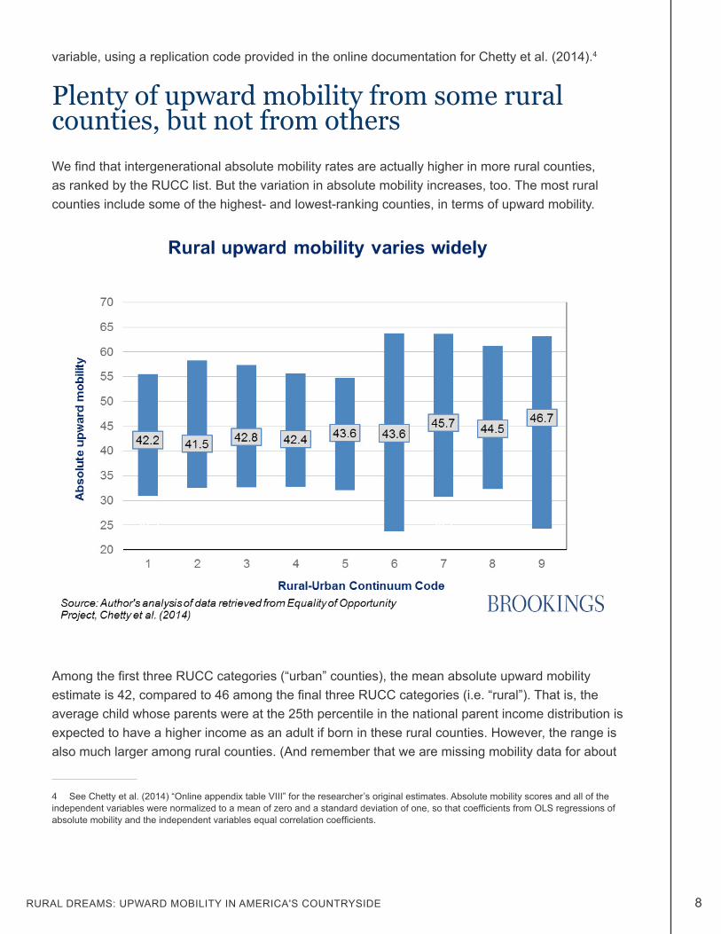
variable, using a replication code provided in the online documentation for Chetty et al. (2014).4

Plenty of upward mobility from some rural counties, but not from othersWe find that intergenerational absolute mobility rates are actually higher in more rural counties, as ranked by the RUCC list. But the variation in absolute mobility increases, too. The most rural counties include some of the highest- and lowest-ranking counties, in terms of upward mobility.

Among the first three RUCC categories (“urban” counties), the mean absolute upward mobility estimate is 42, compared to 46 among the final three RUCC categories (i.e. “rural”). That is, the average child whose parents were at the 25th percentile in the national parent income distribution is expected to have a higher income as an adult if born in these rural counties. However, the range is also much larger among rural counties. (And remember that we are missing mobility data for about

4 See Chetty et al. (2014) “Online appendix table VIII” for the researcher’s original estimates. Absolute mobility scores and all of the independent variables were normalized to a mean of zero and a standard deviation of one, so that coefficients from OLS regressions of absolute mobility and the independent variables equal correlation coefficients.

9 CENTER ON CHILDREN AND FAMILIES AT BROOKINGSKRAUSE, REEVES

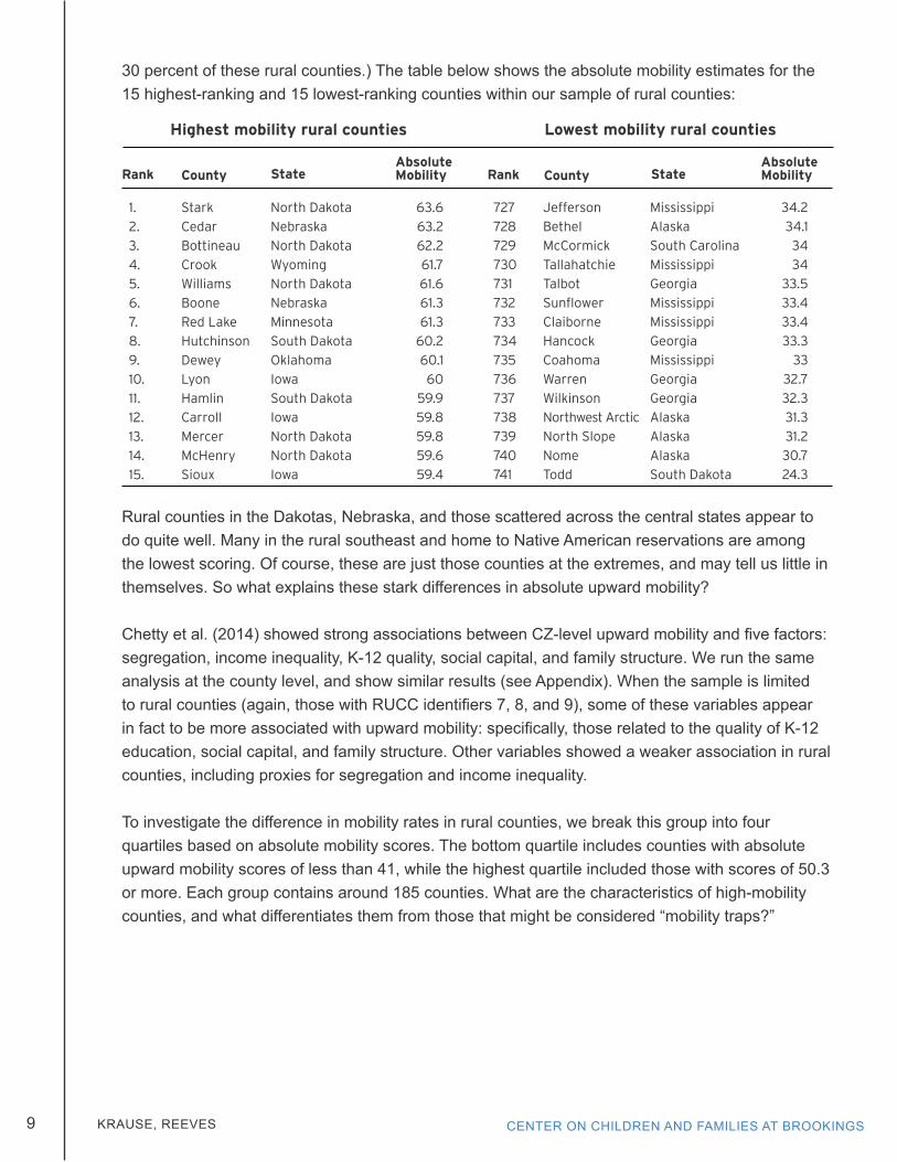
30 percent of these rural counties.) The table below shows the absolute mobility estimates for the 15 highest-ranking and 15 lowest-ranking counties within our sample of rural counties:

Rural counties in the Dakotas, Nebraska, and those scattered across the central states appear to do quite well. Many in the rural southeast and home to Native American reservations are among the lowest scoring. Of course, these are just those counties at the extremes, and may tell us little in themselves. So what explains these stark differences in absolute upward mobility?

Chetty et al. (2014) showed strong associations between CZ-level upward mobility and five factors: segregation, income inequality, K-12 quality, social capital, and family structure. We run the same analysis at the county level, and show similar results (see Appendix). When the sample is limited to rural counties (again, those with RUCC identifiers 7, 8, and 9), some of these variables appear in fact to be more associated with upward mobility: specifically, those related to the quality of K-12 education, social capital, and family structure. Other variables showed a weaker association in rural counties, including proxies for segregation and income inequality. To investigate the difference in mobility rates in rural counties, we break this group into four quartiles based on absolute mobility scores. The bottom quartile includes counties with absolute upward mobility scores of less than 41, while the highest quartile included those with scores of 50.3 or more. Each group contains around 185 counties. What are the characteristics of high-mobility counties, and what differentiates them from those that might be considered “mobility traps?”

CountyRank

1.

2.

3.

4.

5.

6.

7.

8.

9.

10.

11.

12.

13.

14.

15.

StateAbsolute Mobility CountyRank State

Absolute Mobility

Stark

Cedar

Bottineau

Crook

Williams

Boone

Red Lake

Hutchinson

Dewey

Lyon

Hamlin

Carroll

Mercer

McHenry

Sioux

North Dakota

Nebraska

North Dakota

Wyoming

North Dakota

Nebraska

Minnesota

South Dakota

Oklahoma

Iowa

South Dakota

Iowa

North Dakota

North Dakota

Iowa

63.6

63.2

62.2

61.7

61.6

61.3

61.3

60.2

60.1

60

59.9

59.8

59.8

59.6

59.4

727

728

729

730

731

732

733

734

735

736

737

738

739

740

741

Jefferson

Bethel

McCormick

Tallahatchie

Talbot

Sunflower

Claiborne

Hancock

Coahoma

Warren

Wilkinson

Northwest Arctic

North Slope

Nome

Todd

Mississippi

Alaska

South Carolina

Mississippi

Georgia

Mississippi

Mississippi

Georgia

Mississippi

Georgia

Georgia

Alaska

Alaska

Alaska

South Dakota

34.2

34.1

34

34

33.5

33.4

33.4

33.3

33

32.7

32.3

31.3

31.2

30.7

24.3

Highest mobility rural counties Lowest mobility rural counties

10RURAL DREAMS: UPWARD MOBILITY IN AMERICA'S COUNTRYSIDE

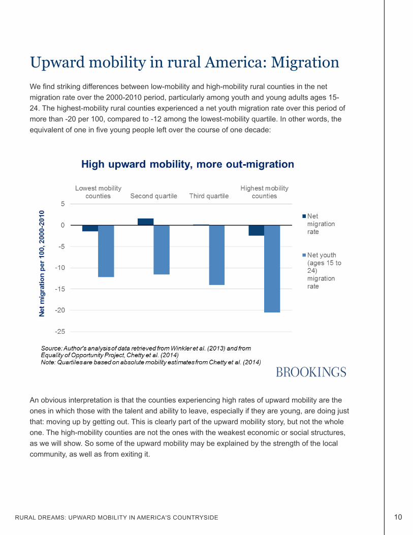
Upward mobility in rural America: MigrationWe find striking differences between low-mobility and high-mobility rural counties in the net migration rate over the 2000-2010 period, particularly among youth and young adults ages 15-24. The highest-mobility rural counties experienced a net youth migration rate over this period of more than -20 per 100, compared to -12 among the lowest-mobility quartile. In other words, the equivalent of one in five young people left over the course of one decade:

An obvious interpretation is that the counties experiencing high rates of upward mobility are the ones in which those with the talent and ability to leave, especially if they are young, are doing just that: moving up by getting out. This is clearly part of the upward mobility story, but not the whole one. The high-mobility counties are not the ones with the weakest economic or social structures, as we will show. So some of the upward mobility may be explained by the strength of the local community, as well as from exiting it.

11 CENTER ON CHILDREN AND FAMILIES AT BROOKINGSKRAUSE, REEVES

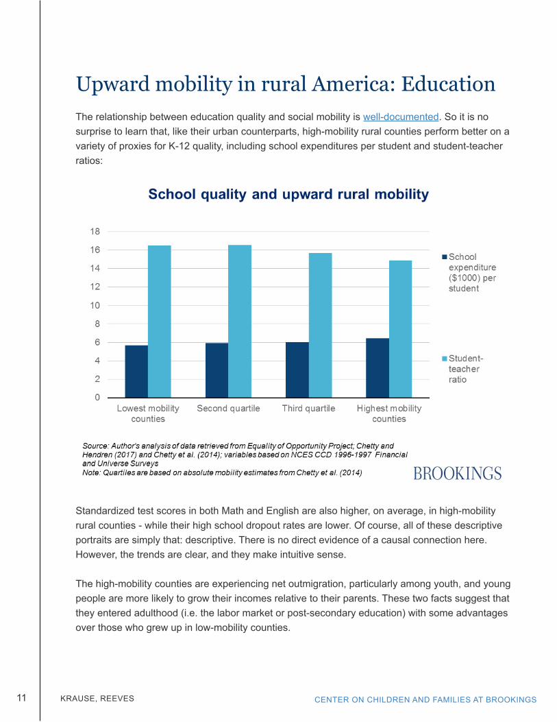
Upward mobility in rural America: Education The relationship between education quality and social mobility is well-documented. So it is no surprise to learn that, like their urban counterparts, high-mobility rural counties perform better on a variety of proxies for K-12 quality, including school expenditures per student and student-teacher ratios:

Standardized test scores in both Math and English are also higher, on average, in high-mobility rural counties - while their high school dropout rates are lower. Of course, all of these descriptive portraits are simply that: descriptive. There is no direct evidence of a causal connection here. However, the trends are clear, and they make intuitive sense. The high-mobility counties are experiencing net outmigration, particularly among youth, and young people are more likely to grow their incomes relative to their parents. These two facts suggest that they entered adulthood (i.e. the labor market or post-secondary education) with some advantages over those who grew up in low-mobility counties.

12RURAL DREAMS: UPWARD MOBILITY IN AMERICA'S COUNTRYSIDE

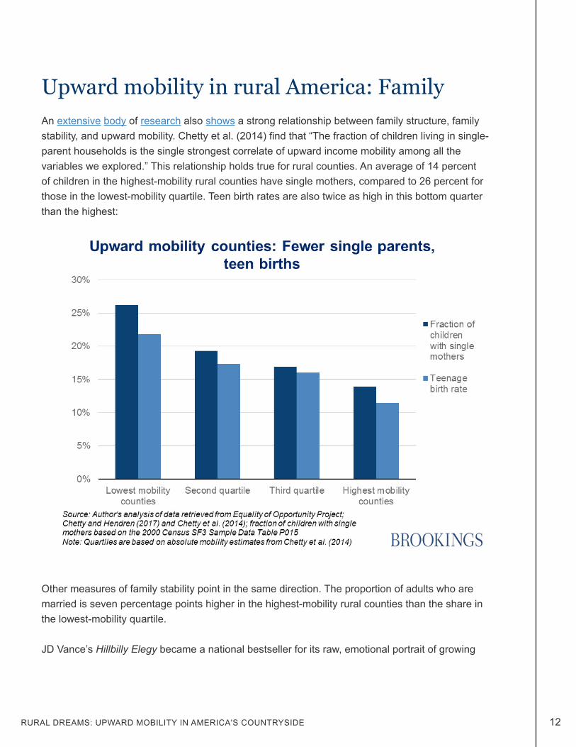
Upward mobility in rural America: FamilyAn extensive body of research also shows a strong relationship between family structure, family stability, and upward mobility. Chetty et al. (2014) find that “The fraction of children living in single-parent households is the single strongest correlate of upward income mobility among all the variables we explored.” This relationship holds true for rural counties. An average of 14 percent of children in the highest-mobility rural counties have single mothers, compared to 26 percent for those in the lowest-mobility quartile. Teen birth rates are also twice as high in this bottom quarter than the highest:

Other measures of family stability point in the same direction. The proportion of adults who are married is seven percentage points higher in the highest-mobility rural counties than the share in the lowest-mobility quartile.

JD Vance’s Hillbilly Elegy became a national bestseller for its raw, emotional portrait of growing

13 CENTER ON CHILDREN AND FAMILIES AT BROOKINGSKRAUSE, REEVES

up in and eventually out of a poor, rural community riddled by drug addiction and instability. Vance became the posterchild for upward mobility out of rural America – eventually graduating from Yale Law School and becoming a principal at a leading Silicon Valley investment firm. Vance attributes his ability to transcend the poor economic prospects of his childhood predominantly to his grandmother (“Mamaw”), who offered him stability. While his mother cycled in in and out of relationships and rehab, Mamaw provided a consistent source of encouragement and a dependable home environment. He writes,

“Now consider the sum of my life after I moved in with Mamaw permanently. At the end of tenth grade, I lived with Mamaw, in her house, with no one else. At the end of eleventh grade, I lived with Mamaw, in her house, with no one else. At the end of twelfth grade, I lived with Mamaw, in her house, with no one else…What I remember most is that I was happy—I no longer feared the school bell at the end of the day, I knew where I’d be living the next month, and no one’s romantic decisions affected my life. And out of that came the opportunities I’ve had for the past twelve years.”

Vance’s story is of course anecdotal (n=1), but it is telling. Family stability looks to be an ingredient for upward mobility. Of all of the variables considered in our own analysis, the “fraction of children with single mothers” produces the largest correlation coefficient (-0.703). If anything, this looks to be even more important in rural counties than in more urban areas: for all counties the coefficient was -0.683.

Upward mobility in rural America: Social capital, segregation, and inequalityChetty et al. (2014) find that proxies for social capital, segregation, and inequality are all highly correlated with mobility. Our analysis confirms that rural counties with lower levels of segregation and inequality and greater levels of social capital also tend to show higher upward mobility: though the association is somewhat weaker than for all counties for certain variables.

One proxy for social capital used by Chetty et al. (2014) is the social capital index developed by Rupasingha and Goetz (2008). This combines a range of indicators from voter turnout rates to participation in community organizations. We find that the average index among the highest-mobility rural counties is 1.48, compared to -0.67 among the lowest-mobility quartile. Other proxies for social capital include the fraction of the population that is religious, and the share of religious adherents is about 24 percentage points higher in high-mobility rural counties (71 percent) than the lowest quartile (47 percent):

14RURAL DREAMS: UPWARD MOBILITY IN AMERICA'S COUNTRYSIDE

Chetty and Hendren (2017) also present county-level indicators for segregation, from proxies for racial and income segregation to the share of the population with a commute of less than 15 minutes. These proxies for segregation are lower in higher-mobility rural counties, though again the association is weaker than among all counties. The “commute” variable is the exception. About 57 percent of the population in the highest-mobility rural counties have a commute of less than 15 minutes, compared to 38 percent of the lowest-mobility quartile: likely a reflection of the strength of the local economy.

Levels of inequality are also higher in low-mobility rural counties. The highest-mobility rural counties have an average Gini coefficient of 0.31, compared to 0.42 for the lowest-mobility quartile.5 Other proxies for inequality show similar trends. The fraction of highest-mobility rural counties classified as “middle class” (between the 25th and 75th percentiles of the national income distribution) is 65 percent, compared to 47 percent in the lowest-mobility counties.

5 The Gini coefficient is a measure of the variation or inequality in incomes, where a lower coefficient implies more equality.

15 CENTER ON CHILDREN AND FAMILIES AT BROOKINGSKRAUSE, REEVES

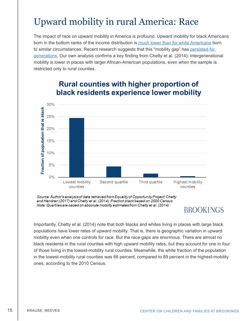
Upward mobility in rural America: RaceThe impact of race on upward mobility in America is profound. Upward mobility for black Americans born in the bottom ranks of the income distribution is much lower than for white Americans born to similar circumstances. Recent research suggests that this “mobility gap” has persisted for generations. Our own analysis confirms a key finding from Chetty et al. (2014): intergenerational mobility is lower in places with larger African-American populations, even when the sample is restricted only to rural counties.

Importantly, Chetty et al. (2014) note that both blacks and whites living in places with large black populations have lower rates of upward mobility. That is, there is geographic variation in upward mobility even when one controls for race. But the race gaps are enormous. There are almost no black residents in the rural counties with high upward mobility rates, but they account for one in four of those living in the lowest-mobility rural counties. Meanwhile, the white fraction of the population in the lowest-mobility rural counties was 66 percent, compared to 89 percent in the highest-mobility ones, according to the 2010 Census.

16RURAL DREAMS: UPWARD MOBILITY IN AMERICA'S COUNTRYSIDE

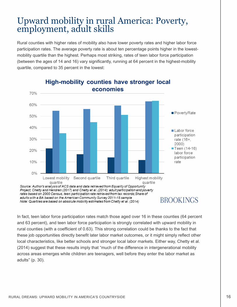
Upward mobility in rural America: Poverty, employment, adult skills Rural counties with higher rates of mobility also have lower poverty rates and higher labor force participation rates. The average poverty rate is about ten percentage points higher in the lowest-mobility quartile than the highest. Perhaps most striking, rates of teen labor force participation (between the ages of 14 and 16) vary significantly, running at 64 percent in the highest-mobility quartile, compared to 35 percent in the lowest:

In fact, teen labor force participation rates match those aged over 16 in these counties (64 percent and 63 percent), and teen labor force participation is strongly correlated with upward mobility in rural counties (with a coefficient of 0.63). This strong correlation could be thanks to the fact that these job opportunities directly benefit later labor market outcomes, or it might simply reflect other local characteristics, like better schools and stronger local labor markets. Either way, Chetty et al. (2014) suggest that these results imply that “much of the difference in intergenerational mobility across areas emerges while children are teenagers, well before they enter the labor market as adults” (p. 30).

17 CENTER ON CHILDREN AND FAMILIES AT BROOKINGSKRAUSE, REEVES

Upward mobility in rural America: Lessons for policyWhat are the policy implications here? If we are serious about improving social mobility, it is clear that we cannot neglect rural areas. Understanding the wide variation in mobility patterns in rural counties may also help to illuminate the policy debate, even in more urban areas. The broad lesson of our findings is that in counties where children are able to prepare well for adult life, they do well: even if, in many cases, this means moving elsewhere. Country boys and girls from modest backgrounds can go on to succeed every bit as much as their city cousins.

We find that growing up in a stable family, attending a good school, and getting some work experience are all more likely for those in the counties showing the higher upward mobility rates. Few surprises here, of course.

We do not propose to set out a comprehensive policy agenda here. And the needs of different places will vary, suggesting the need for a tailored approach. But there are likely to be three key elements of a pro-mobility agenda for rural counties: good schools, broadband access, and access to family planning. These are three “preparedness” approaches - building skills, access, and family stability. There is also a strong case for continuing to support rural areas through community development foundations.

SchoolsSchools matter; and if anything they matter even more in rural than urban areas.6 But as Andy Smarick of the American Enterprise Institute writes, “In many ways, rural schools are fundamentally a mystery to a large segment of K-12 experts.” Smarick points however to a number of successful initiatives underway to improve school quality in rural areas, including philanthropic efforts to increase the number of Advanced Placement (AP) courses and improve career and college counseling. While almost all (97 percent) of urban school districts offer AP courses, barely half of rural districts do. While donor-supported charter-school initiatives have improved options for many poorer families, only about 100 of the 7,000 charter schools open today are in remote rural communities.7 Rural charter schools that operate under rigorous performance-based oversight might be better equipped to tailor resources and curricula to the needs of the local community. Poorer rural areas might struggle to adequately fund their schools. But these are likely to be the areas where improving education is the central ingredient for greater upward mobility. This might be particularly true for areas with larger non-white populations, where investments in human capital have not kept up with the spending in wealthier school districts.

6 The definition of “rural” throughout this section is broader than that used in our analysis (which was limited to counties with RUCC identifiers of 7, 8, and 9). Unless otherwise specified, it generally refers to any area not defined as “urban” or “metropolitan.”7 Here, “remote rural” communities are Census-defined rural territories more than 25 miles from an urbanized area and also more than 10 miles from an urban cluster.

18RURAL DREAMS: UPWARD MOBILITY IN AMERICA'S COUNTRYSIDE

BroadbandSkills and learning are vital: but so is connection. As Darrell West and Jack Karsten explain, “The rural/urban ‘digital divide’ in access severely limits rural populations from taking advantage of a critical component of modern life.” This digital divide also makes it much more challenging for students to get 21st century educations. As West and Karsten go on:

“Rural schools lack access to high-speed fiber and pay more than twice as much for bandwidth. In a growing world of personalized online curricula, internet-based research, and online testing, this severely restricts rural students from educational opportunities their urban counterparts may enjoy.”

Four in ten rural Americans lacked access to the FCC’s benchmark broadband service, compared to only 4 percent of the urban population, according to the Federal Communications Commission (FCC)’s 2016 Broadband Progress Report.

Just as President Roosevelt’s Rural Electrification Administration delivered electricity to rural America in the 1930s and, with it, the “economic benefits provided by power,” so too could President Trump’s administration seek to eliminate the digital divide to ensure the economic benefits provided by connection. The promised federal infrastructure plan offers a good opportunity to bring broadband to unserved areas, and a bipartisan group of 71 members of Congress have signed a letter to President Trump urging him to include investments in rural broadband connectivity in his infrastructure proposal.8

Family planningThe strong link between family structure and upward mobility in rural America should come as no surprise - the relationship between family instability and poor educational and labor market outcomes is well-documented. Family stability results from a wide range of factors, of course, including economic security, financial resources, social norms, and workplace flexibility. But one factor that very clearly contributes to instability, and which can be addressed through policy, is unplanned pregnancy. We find a strong association between teen birth rates and upward mobility in rural counties. The impressive decline in teen pregnancy over the past several decades is largely thanks to the improved use of contraceptives, particularly long-acting reversible contraceptives (LARCs) like IUDs and implants. But while the teen birth rate fell 50 percent in large urban counties between 2007 and 2015, it only fell 37 percent in rural counties during this time frame. As of 2015, the teen birth rate per 1,000 girls ages 15 to 19 was 31 in rural counties, compared to 22 for the entire country. Rural

8 As they write: “Simply put, rural communities cannot attract and retain businesses and human resources if they are insufficiently connected. Broadband allows rural Americans to communicate with friends and families and access entertainment. It provides businesses access to global customers to reach and drive economic development. It facilitates agricultural efficiency for farmers, supplies students and teachers with unlimited access to educational materials, and ensures a timely response to health and safety emergencies by first responders.”

19 CENTER ON CHILDREN AND FAMILIES AT BROOKINGSKRAUSE, REEVES

Americans face unique obstacles to receiving health care compared to those living in urban areas. The National Campaign to Prevent Teen and Unplanned Pregnancy points to the problem of access to health services and health insurance in rural areas. Efforts to reduce these disparities are likely to include the protection or expansion of health coverage (particularly publicly-funded health insurance for low-income families), supporting publicly funded clinics, and promoting the availability of the full range of contraceptive options, including LARCS. School-based health centers and online programs could also help to reduce transportation barriers in more isolated areas. (Of course, online platforms will only prove effective if complemented by expanded access to broadband in some regions.)

ConclusionOur findings show that on average, rural counties have mobility rates as high as their urban counterparts, but that there is much more variation, too. America’s rural counties exhibit some of the highest rates of upward absolute mobility in the country, as well as some of the lowest. There are some clear differences between high-mobility counties and those that might be considered “mobility traps,” in terms of education, work experience, family stability, and out-migration. Rural counties in the Southeast tend to have much lower intergenerational mobility scores than those in the Great Plains, which generally perform quite well. These regional differences might be explained by disparities in things like investments in primary education and patterns of family structure we witness at the county level.

The striking link to out-migration suggests that, at least to some extent, upward mobility does require mobility of the geographical kind, too. There is a long-running debate in policy circles between “place-based” and “people-based” approaches. Generally, economists lean against attempts to prop up places that are in economic decline, for example through subsidies to businesses. Better to equip individuals with the skills they need to thrive, and perhaps assist them in moving on to a new, opportunity-rich, city. Many of our findings support this people-centric as opposed to place-oriented approach. Alongside the investments in education, internet access, and family planning discussed above, there is a case for providing some assistance to those who wish to leave rural areas for greater opportunities elsewhere. As Patrick Kline and Enrico Moretti explain, credit constraints may prevent some individuals from relocating. Some individuals with no access to credit may be forced to remain in distressed areas or working in low-wage jobs even when it would likely be better, at least in economic terms, for them to seek employment elsewhere. In certain situations, mobility vouchers could help overcome these credit constraints. But the “people vs. place” contrast should not be overstated. It is easier for individuals to acquire the skills, credentials, and experience needed for upward mobility in a place with a stronger

20RURAL DREAMS: UPWARD MOBILITY IN AMERICA'S COUNTRYSIDE

economy and social fabric. While migration is an important part of the mobility story, it cannot be the whole story. When Chetty et al. (2014) ranked the largest 50 commuting zones by intergenerational mobility, nobody recommended that we move all of the residents of Charlotte and Atlanta (the bottom scorers) to Pittsburgh and Salt Lake City (the highest scorers). Instead, community leaders in Charlotte created a “citywide task force aimed at increasing opportunities for poor children.” This kind of local-centric response will also be critical to bolstering opportunity in rural America: for those who choose to leave, but also for those who prefer to stay.

21 CENTER ON CHILDREN AND FAMILIES AT BROOKINGSKRAUSE, REEVES

AppendixThe following table depicts the results of the OLS regressions run using a code based on that used for Chetty et al. (2014), “Online Appendix Table IIIV.” The dependent variable (absolute upward mobility) is the same as that used in Chetty et al. (2014). The independent variables (with the exception of net migration rates) were retrieved from the online data tables available for Chetty and Hendren (2017). See Chetty and Hendren (2017), “Online appendix table XV: Commuting zone and county characteristics: Definitions and data sources” for a more detailed explanation of variable definitions and sources. Net migration rates were retrieved from Winkler et al. (2013).

22RURAL DREAMS: UPWARD MOBILITY IN AMERICA'S COUNTRYSIDE

Chetty et al. (2014) note, “Each cell reports estimates from OLS regressions of a measure of mobility on the variable listed in each row, normalizing both the dependent and independent variables to have mean 0 and standard deviation 1 in the estimation sample, so that univariate regression coefficients equal correlation coefficients.” The first column of coefficients shows the results from a regression run for all counties, while the second column is the result of one run only for counties with RUCC identifiers 7, 8, and 9. We also ran the same regressions controlling for state fixed effects and with population weights, though the coefficients from those OLS regressions are omitted here. They are available upon request.

23 CENTER ON CHILDREN AND FAMILIES AT BROOKINGSKRAUSE, REEVES

ReferencesChetty, Raj and Nathaniel Hendren, “The impacts of neighborhoods on intergenerational mobility II: County-level estimates,” The Equality of Opportunity Project, May 2017, http://www.equality-of-op-portunity.org/assets/documents/movers_paper2.pdf.

Chetty, Raj, Nathaniel Hendren, Patrick Kline, and Emmanuel Saez, “Where is the land of opportu-nity? The geography of intergenerational mobility in the United States,” The Equality of Opportunity Project, June 2014, http://www.equality-of-opportunity.org/assets/documents/mobility_geo.pdf.

Rupasingha, Anil and Stephen J. Goetz, “US County-Level Social Capital Data, 1990-2005.” The Northeast Regional Center for Rural Development, Penn State University, University Park, PA, 2008.

Winkler, Richelle, Kenneth M. Johnson, Cheng Cheng, Jim Beaudoin, Paul R. Voss, and Katherine J. Curtis, “Age-Specific Net Migration Estimates for US Counties, 1950-2010,” Applied Population Laboratory, University of Wisconsin- Madison, 2013, accessed July 2, 2017 from http://www.netmi-gration.wisc.edu/.