171
SAMPLING VEGETATION ATTRIBUTES INTERAGENCY TECHNICAL REFERENCE
| Date post: | 02-Jan-2017 |
| Category: |
Documents |
| Upload: | phungtuong |
| View: | 231 times |
| Download: | 2 times |
SAMPLING VEGETATIONATTRIBUTES
INTERAGENCY TECHNICAL REFERENCE

Supersedes BLM Technical Reference 4400-4, Trend Studies, dated May 1985
Edited, designed, and produced by the Bureau of Land Management’sNational Applied Resource Sciences Center
BLM/RS/ST-96/002+1730
Sampling Vegetation AttributesInteragency Technical Reference
Cooperative Extension Service
U.S. Department of Agriculture— Forest Service —
Natural Resource Conservation Service,Grazing Land Technology Institute
U.S. Department of the Interior— Bureau of Land Management —
1996Revised in 1997, and 1999

TABLE OF CONTENTS
SAMPLING VEGETATION ATTRIBUTESInteragency Technical Reference
By (In alphabetical order)
Technical Reference 1734-4copies available from
Bureau of Land ManagementNational Business Center
BC-650BP.O. Box 25047
Denver, Colorado 80225-0047
Bill CoulloudonRangeland Management Spec.Bureau of Land ManagementPhoenix, Arizona
Kris Eshelman (deceased)Rangeland Management Spec.Bureau of Land ManagementReno, Nevada
James GianolaWildhorse and Burro Spec.Bureau of Land ManagementCarson City, Nevada
Ned HabichRangeland Management Spec.Bureau of Land ManagementDenver Colorado
Lee HughesEcologistBureau of Land ManagementSt. George, Utah
Curt JohnsonRangeland Management Spec.Forest Service Region 4Ogden Utah
Mike PellantRangeland EcologistBureau of Land ManagementBoise, Idaho
Paul PodbornyWildlife BiologistBureau of Land ManagementEly, Nevada
Allen RasmussenRangeland Management Spec.Cooperative Extension ServiceUtah State UniversityLogan, UT
Ben RoblesWildlife BiologistBureau of Land ManagementSafford, Arizona
Pat ShaverNatural Resource Conservation ServiceRangeland Management Spec.Corvallis, Oregon
John SpeharRangeland Management Spec.Bureau of Land ManagementRawlins, Wyoming
John WilloughbyState BiologistBureau of Land ManagementSacramento, California

TABLE OF CONTENTS
TABLE OF CONTENTSPage
I. PREFACE ..................................................................................................................i
II. INTRODUCTION ...................................................................................................1A. Terms and Concepts ...........................................................................................1B. Techniques Not Addressed ..................................................................................2C. Guidelines ...........................................................................................................3D. Location of Study Sites .......................................................................................3E. Key Species ........................................................................................................ 4F. General Observations ..........................................................................................5G. Coordination .......................................................................................................6H. Electronic Data Recorders ..................................................................................6I. Reference Areas ..................................................................................................6
III. STUDY DESIGN AND ANALYSIS..........................................................................7A. Planning the Study ..............................................................................................8B. Statistical Considerations ..................................................................................12C. Other Important Considerations .......................................................................22
IV. ATTRIBUTES .........................................................................................................23A. Frequency .........................................................................................................23B. Cover ..............................................................................................................25C. Density .............................................................................................................26D. Production ........................................................................................................27E. Structure ...........................................................................................................28F. Composition .....................................................................................................28
V. METHODS ........................................................................................................... 31A. Photographs ......................................................................................................31B. Frequency Methods ...........................................................................................37C. Dry Weight Rank Method .................................................................................50D. Daubenmire Method ........................................................................................55E. Line Intercept Method ......................................................................................64F. Step-Point Method ............................................................................................70G. Point-Intercept Method ....................................................................................78H. Cover Board Method ........................................................................................86I. Density Method ................................................................................................94J. Double-Weight Sampling ................................................................................102K. Harvest Method ..............................................................................................112L. Comparative Yield Method .............................................................................116M. Visual Obstruction Method - Robel Pole ........................................................123N. Other Methods ...............................................................................................130
VI. GLOSSARY OF TERMS ......................................................................................131
VII. REFERENCES ......................................................................................................139
APPENDIXES ...............................................................................................................149Appendix A Study Location and Documentation Data Form........................................149Appendix B Study and Photograph Identification .........................................................153Appendix C Photo Identification Label .........................................................................157Appendix D Selecting Random Samples (Using Random Number Tables) ....................161

TABLE OF CONTENTS
TABLE OF CONTENTS (continued)Illustration Title PageNumber
1 ........ Photo Plot - 3 X 3 Plot Frame Diagram .........................................................342 ........ Photo Plot - 5 X 5 Plot Frame Diagram .........................................................353 ........ Permanent Photo Plot Location......................................................................364 ........ Frequency Form ....................................................................................... 44-455 ........ Nested Frequency Form ........................................................................... 46-476 ........ Frequency Frame ............................................................................................487 ........ Nested Plot Frame..........................................................................................498 ........ Dry Weight Rank Form ............................................................................ 53-549 ........ Daubenmire Form.................................................................................... 59-6010 ...... Daubenmire Summary Form ................................................................... 61-6211 ...... Daubenmire Frame ........................................................................................6312 ...... Line Intercept Form ................................................................................. 68-6913 ...... Cover Data Form ..................................................................................... 75-7614 ...... Sample Units (Hits) and Recording Procedures .............................................7715 ...... Examples of Sighting Devices ........................................................................8316 ...... Examples of Pin Frames .................................................................................8417 ...... Example of a Point Frame ..............................................................................8518 ...... Cover Board Method: Density Board Form ............................................. 89-9019 ...... Cover Board Method: Profile Board Form ............................................... 91-9220 ...... Examples of Cover Boards .............................................................................9321 ...... Density Form ....................................................................................... 100-10122 ...... Production Form .................................................................................. 109-11023 ...... Weight Estimate Quadrat.............................................................................11124 ...... Comparative Yield Form ...................................................................... 121-12225 ...... Robel Pole Form................................................................................... 127-12826 ...... Robel Pole ....................................................................................................129

i
PREFACE
DEDICATIONThis publication is dedicated to the memory of Kristen R. Eshelman, who
contributed tremendously to its development and preparation. Through-
out his career, Kris was instrumental in producing numerous technical
references outlining procedures for rangeland inventory, monitoring, and
the evaluation of rangeland data. Through his efforts, resource specialists
were provided with the tools to improve the public rangelands for the
benefit of rangeland users and the American public.
DEDICATION
iii
PREFACE
I. PREFACEThe intent of this interagency monitoring guide is to provide the basis for consistent,uniform, and standard vegetation attribute sampling that is economical, repeatable,statistically reliable, and technically adequate. While this guide is not all inclusive, it doesinclude the primary sampling methods used across the West. An omission of a particularsampling method does not mean that the method is not valid in specific locations; it simplymeans that it is not widely used or recognized throughout the western states. (See SectionV.N, Other Methods.)
Proper use and management of our rangeland resources has created a demand for uniformityand consistency in rangeland health measurement methods. As a result of this interest, theUSDI Bureau of Land Management (BLM) and USDA Forest Service met in late 1992 andagreed to establish an interagency technical team to jointly oversee the development andpublishing of vegetation sampling field guides.
The 13-member team currently includes representatives from the Forest Service, BLM, theGrazing Land Technology Institute of the Natural Resource Conservation Service (NRCS),and the Cooperative Extension Service.
The interagency technical team first met in January 1994 to evaluate the existing rangelandmonitoring techniques described in BLM’s Trend Studies, Technical Reference TR 4400-4. Theteam spent 2 years reviewing, modifying, adding to, and eliminating techniques for thisinteragency Sampling Vegetation Attributes technical reference. Feedback from numerousreviewers, including field personnel, resulted in further refinements.

1
INTRODUCTION
II. INTRODUCTIONIdentifying the appropriate sampling technique first requires the identification of the propervegetation characteristic or attribute to measure. To do this the examiner must considerobjectives, life form (grass, forb, shrub, or tree), distribution patterns of individuals of aspecies, distribution patterns between species (community mosaic pattern), efficiency of datacollection from an economic standpoint, and accuracy and precision of the data.
Permittees, lessees, other rangeland users, and interested publics should be consulted andencouraged to participate in the collection and analysis of monitoring data. Those individualsor groups interested in helping to collect data should be trained in the technique used in thespecific management unit.
This document deals with the collection of vegetation data. The interpretation of that datawill be addressed in other documents. This document does not address interpreting vegeta-tion data for adjusting livestock numbers or making other management decisions.
A. Terms and Concepts The following terms require an expanded discussionbeyond the scope of the Glossary of Terms:
1. Inventory Inventory is the systematic acquisition and analysis of informationneeded to describe, characterize, or quantify vegetation. As might be expected,data for many different vegetation attributes can be collected. Inventories can beused not only for mapping and describing ecological sites, but also for determiningecological status, assessing the distribution and abundance of species, and establish-ing baseline data for monitoring studies.
2. Population A population (used here in the statistical, not the biological, sense)is a complete collection of objects (usually called units) about which one wishes tomake statistical inferences. Population units can be individual plants, points, plots,quadrats, or transects.
3. Sampling Unit A sampling unit is one of a set of objects in a sample that isdrawn to make inferences about a population of those same objects. A collectionof sampling units is a sample. Sampling units can be individual plants, points,plots, quadrats, or transects.
4. Sample A sample is a set of units selected from a population used to estimatesomething about the population (statisticians call this making inference about thepopulation). In order to properly make inferences about the population, the unitsmust be selected using some random procedure (see Technical Reference, Measuring& Monitoring Plant Populations). The units selected are called sampling units.
5. Sampling Sampling is a means by which inferences about a plant communitycan be made based on information from an examination of a small proportion ofthat community. The most complete way to determine the characteristics of apopulation is to conduct a complete enumeration or census. In a census, eachindividual unit in the population is sampled to provide the data for the aggregate.This process is both time-consuming and costly. It may also result in inaccurate

INTRODUCTION
2
values when individual sampling units are difficult to identify. Therefore, the bestway to collect vegetation data is to sample a small subset of the population. If thepopulation is uniform, sampling can be conducted anywhere in the population.However, most vegetation populations are not uniform. It is important that databe collected so that the sample represents the entire population. Sample design isan important consideration in collecting representative data. (See Section III.)
6. Shrub Characterization Shrub characterization is addressed here since it isnot covered in most of the techniques in this technical reference. Shrub character-ization is the collection of data on the shrub and tree component of a vegetationcommunity. Attributes that could be important for shrub characterization areheight, volume, foliage density, crown diameter, form class, age class, and totalnumber of plants by species (density). Another important feature of shrub charac-terization is the collection of data on a vertical as well as a horizontal plane.Canopy layering is also important. The occurrence of individual species and theextent of canopy cover of each species is recorded in layers. The number of layerschosen should represent the herbaceous layer, the shrub layer, and the tree layer,though additional layers can be added if needed.
7. Trend Trend refers to the direction of change. Vegetation data are collected atdifferent points in time on the same site and the results are then compared to detecta change. Trend is described as moving “towards meeting objectives,” “away frommeeting objectives,” “not apparent,” or “static.” Trend data are important in deter-mining the effectiveness of on-the-ground management actions. Trend data indicatewhether the rangeland is moving towards or away from specific objectives. Thetrend of a rangeland area may be judged by noting changes in vegetation attributessuch as species composition, density, cover, production, and frequency. Trend data,along with actual use, authorized use, estimated use, utilization, climate, and otherrelevant data, are considered in evaluating activity plans.
8. Vegetation Attributes Vegetation attributes are quantitative features or charac-teristics of vegetation that describe how many, how much, or what kind of plantspecies are present. The most commonly used attributes are:
Frequency ProductionCover StructureDensity Species Composition
B. Techniques Not Addressed The following are not included in this document:
• Riparian Monitoring
• Monitoring Using Aerial Photography
• Special Status Plant Monitoring
• Weight Estimate and Ocular Reconnaissance Methods
• Soil Vegetation Inventory Method
• Community Structure Analysis Method
• Photo Plot Method
3
INTRODUCTION
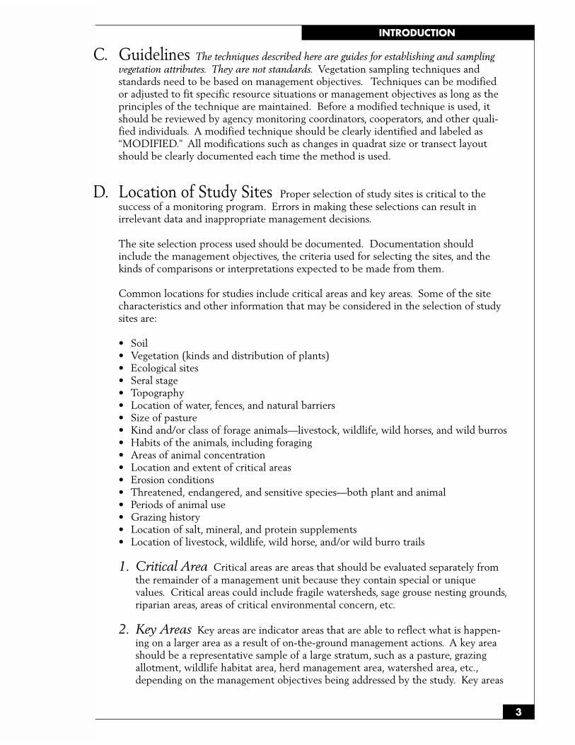
C. Guidelines The techniques described here are guides for establishing and samplingvegetation attributes. They are not standards. Vegetation sampling techniques andstandards need to be based on management objectives. Techniques can be modifiedor adjusted to fit specific resource situations or management objectives as long as theprinciples of the technique are maintained. Before a modified technique is used, itshould be reviewed by agency monitoring coordinators, cooperators, and other quali-fied individuals. A modified technique should be clearly identified and labeled as“MODIFIED.” All modifications such as changes in quadrat size or transect layoutshould be clearly documented each time the method is used.
D. Location of Study Sites Proper selection of study sites is critical to thesuccess of a monitoring program. Errors in making these selections can result inirrelevant data and inappropriate management decisions.
The site selection process used should be documented. Documentation shouldinclude the management objectives, the criteria used for selecting the sites, and thekinds of comparisons or interpretations expected to be made from them.
Common locations for studies include critical areas and key areas. Some of the sitecharacteristics and other information that may be considered in the selection of studysites are:
• Soil• Vegetation (kinds and distribution of plants)• Ecological sites• Seral stage• Topography• Location of water, fences, and natural barriers• Size of pasture• Kind and/or class of forage animals—livestock, wildlife, wild horses, and wild burros• Habits of the animals, including foraging• Areas of animal concentration• Location and extent of critical areas• Erosion conditions• Threatened, endangered, and sensitive species—both plant and animal• Periods of animal use• Grazing history• Location of salt, mineral, and protein supplements• Location of livestock, wildlife, wild horse, and/or wild burro trails
1. Critical Area Critical areas are areas that should be evaluated separately fromthe remainder of a management unit because they contain special or uniquevalues. Critical areas could include fragile watersheds, sage grouse nesting grounds,riparian areas, areas of critical environmental concern, etc.
2. Key Areas Key areas are indicator areas that are able to reflect what is happen-ing on a larger area as a result of on-the-ground management actions. A key areashould be a representative sample of a large stratum, such as a pasture, grazingallotment, wildlife habitat area, herd management area, watershed area, etc.,depending on the management objectives being addressed by the study. Key areas

INTRODUCTION
4
represent the “pulse” of the rangeland. Proper selection of key areas requiresappropriate stratification. Statistical inference can only be applied to the stratifica-tion unit.
a Selecting Key Areas The most important factors to consider when selectingkey areas are the management objectives found in land use plans, coordinatedresource management plans, and/or activity plans. An interdisciplinary teamshould be used to select these areas. In addition, permittees, lessees, and otherinterested publics should be invited to participate, as appropriate, in selectingkey areas. Poor information resulting from improper selection of key areas leadsto misguided decisions and improper management.
b Criteria for Selecting Key Areas The following are some criteria that shouldbe considered in selecting key areas. A key area:
• Should be representative of the stratum in which it is located.
• Should be located within a single ecological site and plant community.
• Should contain the key species where the key species concept is used.
• Should be capable of and likely to show a response to management actions.This response should be indicative of the response that is occurring on thestratum.
c Number of Key Areas The number of key areas selected to represent a stratumideally depends on the size of the stratum and on data needs. However, thenumber of areas may ultimately be limited by funding and personnel constraints.
d Objectives Objectives should be developed so that they are specific to the keyarea. Monitoring studies can then be designed to determine if these objectives arebeing met.
e Mapping Key Areas Key areas should be accurately delineated on aerialphotos and/or maps. Mapping of key areas will provide a permanent record oftheir location.
E. Key Species Key species are generally an important component of a plantcommunity. Key species serve as indicators of change and may or may not be foragespecies. More than one key species may be selected for a stratum, depending onobjectives and data needs. In some cases, problem plants (poisonous, etc.) may beselected as key species. Key species may change from season to season.
The process used to select key species should be documented. Documentation shouldinclude the management objectives, the criteria used for selecting species, and the kindsof comparisons or interpretations expected to be made from them.
a Selecting Key Species Selection of key species should be tied directly toobjectives in land-use plans, coordinated resource management plans, andactivity plans. This selection depends upon the plant species in the presentplant community, the present ecological status, and the potential natural com-munities for the specific sites. An interdisciplinary team should be used in

5
INTRODUCTION
selecting key species to ensure that data needs of the various resources are met.In addition, interested publics should be invited to participate, as appropriate, inselecting these species (see Section II.G).
b Considerations in Selecting Key Species The following points should beconsidered in selecting key species:
• Changes in density, frequency, reproduction, etc., of key species on key areasare assumed to reflect changes in these species on the entire stratum.
• The forage value of key species may be of secondary or no importance. Forexample, watershed protection may require selection of plants as key specieswhich protect the watershed but are not the best forage species. In somecases, threatened, endangered, or sensitive species that have no particularforage value may be selected as key species.
• Any foraging use of the key species on key areas is assumed to reflect forag-ing use of that species on the entire stratum.
• Depending on the selected management strategy and/or periods of use, keyspecies may be foraged during the growing period, after maturity, or both.
• In areas of yearlong grazing use and in areas where there is more than oneuse period, several key species may be selected to sample. For example, onan area with both spring and summer grazing use, a cool season plant may bethe key species during the spring, while a warm season plant may be the keyspecies during the summer.
• Selection of several key species may be desirable when adjustments in livestockgrazing use are anticipated. This is especially true if more than one plant speciescontributes a major portion of the forage base of the animals using the area(Smith 1965).
c. Key Species on Depleted Rangelands The key species selected should bepresent on each key area on which monitoring studies are conducted; however,on depleted rangelands these species may be sparse or absent. In this situationit may be necessary to conduct monitoring studies on other species. Datagathered on non-key species must be interpreted on the basis of effects on theestablishment and subsequent response of the key species. It should also beverified that the site is ecologically capable of producing the key species.
F. General Observations General observations can be important when con-ducting evaluations of grazing allotments, wildlife habitat areas, wild horse and burroherd management areas, watershed areas, or other designated management areas.Such factors as rodent use, insect infestations, animal concentrations, fire, vandalism,and other uses of the sites can have considerable impact on vegetation and soil re-sources. This information is recorded on the reverse side of the study method forms oron separate pages, as necessary.
INTRODUCTION
6
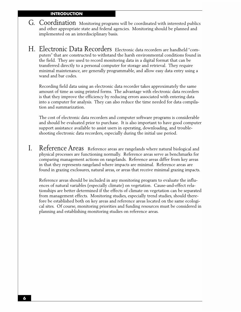
G. Coordination Monitoring programs will be coordinated with interested publicsand other appropriate state and federal agencies. Monitoring should be planned andimplemented on an interdisciplinary basis.
H. Electronic Data Recorders Electronic data recorders are handheld “com-puters” that are constructed to withstand the harsh environmental conditions found inthe field. They are used to record monitoring data in a digital format that can betransferred directly to a personal computer for storage and retrieval. They requireminimal maintenance, are generally programmable, and allow easy data entry using awand and bar codes.
Recording field data using an electronic data recorder takes approximately the sameamount of time as using printed forms. The advantage with electronic data recordersis that they improve the efficiency by reducing errors associated with entering datainto a computer for analysis. They can also reduce the time needed for data compila-tion and summarization.
The cost of electronic data recorders and computer software programs is considerableand should be evaluated prior to purchase. It is also important to have good computersupport assistance available to assist users in operating, downloading, and trouble-shooting electronic data recorders, especially during the initial use period.
I. Reference Areas Reference areas are rangelands where natural biological andphysical processes are functioning normally. Reference areas serve as benchmarks forcomparing management actions on rangelands. Reference areas differ from key areasin that they represents rangeland where impacts are minimal. Reference areas arefound in grazing exclosures, natural areas, or areas that receive minimal grazing impacts.
Reference areas should be included in any monitoring program to evaluate the influ-ences of natural variables (especially climate) on vegetation. Cause-and-effect rela-tionships are better determined if the effects of climate on vegetation can be separatedfrom management effects. Monitoring studies, especially trend studies, should there-fore be established both on key areas and reference areas located on the same ecologi-cal sites. Of course, monitoring priorities and funding resources must be considered inplanning and establishing monitoring studies on reference areas.
7
STUDY DESIGN AND ANALYSIS
III. STUDY DESIGN AND ANALYSIS
The rangeland monitoring methods described in Section V have a number of commonelements. Those that relate to permanently marking and documenting the study locationare described in detail below.
Also discussed in this section are statistical considerations (target populations, randomsampling, systematic sampling, confidence intervals, etc.) and other important factors (prop-erly identifying plant species and training people so they follow the correct procedures).
It is important to read this chapter before referring to the specific methods described inSection V, since the material covered here will not be repeated for each of them.
Permanently Marking the Study Location Permanently mark the location of each studyby means of a reference post (steel post) placed about 100 feet from the actual studylocation. Record the bearing and distance from the post to the study location. An alter-native is to select a reference point, such as a prominent natural or man-made feature, andrecord the bearing and distance from that point to the study location. If a post is used, itshould be tagged to indicate that it marks the location of a monitoring study and shouldnot be disturbed.
Permanently mark the study location itself by driving angle iron stakes into the ground atrandomly selected starting points. The baseline technique requires that both ends of thebaseline be permanently staked. With the macroplot technique, a minimum of threecorners need to be permanently staked. If the linear technique is used, only the beginningpoint of the study needs to be permanently staked. Establish the study according to thedirections found in Section III.A.2 beginning on page 8.
Paint the transect location stake with brightly colored permanent spray paint (yellow ororange) to aid in relocation. Repaint this stake when subsequent readings are made.
Study Documentation Document the study and transect locations, number of transects,starting points, bearings, length, distance between transects, number of quadrats, samplinginterval, quadrat frame size, size of plots in a nested plot frame technique, number ofcover points per quadrat frame, and other pertinent information concerning a study on theStudy Location and Documentation Data form (see Appendix A). For studies that use abaseline technique, record the location of each transect along the baseline and the direc-tion (left or right).
Be sure to document the exact location of the study site and the directions for relocatingit. For example: 1.2 miles from the allotment boundary fence on the Old County Line Road.The reference post is on the south side of the road, 50 feet from the road.
Plot the precise location of the study on detailed maps and/or aerial photos.
STUDY DESIGN AND ANALYSIS
8
A. Planning the Study Proper planning is by far the most important part of amonitoring study. Much wasted time and effort can be avoided by proper planning.A few important considerations are discussed below. The reader should refer toTechnical Reference, Measuring & Monitoring Plant Populations, for a more completediscussion of these important steps.
1. Identify Objectives Based on land use and activity plans, identify objectivesappropriate for the area to be monitored. The intent is to evaluate the effects ofmanagement actions on achieving objectives by sampling specific vegetationattributes.
2. Design the Study The number of quadrats, points, or transects (sample size)needed depends on the objectives and the efficiency of the sampling design. It shouldbe known before beginning the study how the data will be analyzed. The frequency ofdata collection (e.g., every year, every other year, etc.) and data sheet design should bedetermined before studies are implemented. The sample data sheets included witheach method (following the narrative) are only examples of data forms. Fieldoffices have the option to modify these forms or develop their own.
All of the methods described in this document can be established using the followingtechniques:
a Baseline A baseline is established by stretching a tape measure of any desiredlength between two stakes (figure 1). For an extremely long baseline, interme-diate stakes can be used to ensure proper alignment. It is recommended thatmetric measurement be used. Individual transects are then run perpendicular tothe baseline at random locations along the tape. The location of quadrats alongthese transects can be either measured or paced. Transects can all be run in thesame direction, in which case the baseline forms one of the outer boundaries ofthe sampled area, or in two directions, in which case the baseline runs throughthe center of the sampled area. If transects are run in two directions, the direc-tion for each individual transect should be determined randomly. (Directionsfor randomly selecting the location of transects to be run off of a baseline usinga random numbers table are given in Appendix D). Quadrats or observationpoints are spaced at specified distances along the transect. This study design isintended to randomly sample a specified area. The area to be sampled can beexpanded as necessary by lengthening the baseline and/or increasing the lengthbetween quadrats or sampling points.
This design may need to be modified for riparian areas or other areas where thearea to be sampled is long and narrow. For these areas, a single linear transectmay be more appropriate.
b Macroplot The concept with this type of design is to allow every area withinthe study site or sample area to have an equal chance to be sampled. Amacroplot is a large square or rectangular study site. The size of the macroplotwill depend on the size of the study site. The macroplot should encompassmost of the study site. From the standpoint of statistical inference, it is best,once the macroplot boundaries have been determined, to redefine the study siteto equal the macroplot. Examples of macroplot sizes are 50 m x 100 m, 100 mx 100 m, and 100 m x 200 m, but much larger macroplots can be used to coverlarger study sites. Macroplot size and shape should be tailored to each situation.

9
STUDY DESIGN AND ANALYSIS
Transect 1
Transect 2
Transect 3
∆∆
Baseline End Point Stake
100-Meter Baseline Tape
Study Layout
Photo plots may be
permanently located
anywhere along the
baseline tape.
Figure 1. Study layout for the baseline technique.
∆
∆ Study Location Stake
Baseline Beginning Point Stake

STUDY DESIGN AND ANALYSIS
10
Macroplot size also depends on the size and shape of the quadrats that will beused to sample it. The sides of the macroplot should be of dimensions that aremultiples of the sides of the quadrats.
(1) Macroplot layout Pick one corner of the macroplot to serve as the beginningfor sampling purposes. Drive an angle iron location stake into the groundat this corner. Determine the bearing of the macroplot side that will serveas the x-axis, run a tape in that direction and put an angle iron stake at theselected distance. This serves as another corner of the macroplot. Leavethe x-axis tape in place for sampling purposes. Return to the origin anddetermine the bearing of the y-axis, which will be perpendicular to the x-axis. Run a second tape along the y-axis and put an angle iron stake in theground at the selected distance. This serves as the third corner of themacroplot. If desired, a fourth stake may be placed at the remainingcorner, but this is not necessary for sampling since sampling will be doneusing the two tapes serving as the x- and y-axes. See Figure 2 for an ex-ample. Leave the tapes in place until the first year’s sampling is completed.
Be sure to document the directions of the x- and y-axes so that themacroplot can be reconstructed if one of the angle iron stakes is missing.
(2) Quadrat locations Quadrats are located in the macroplot using a coordi-nate system to identify the lower left-hand corner of each quadrat.
(a) For example it has been determined from the pilot study that 40samples are needed using a 1 m by 16 m quadrat. The quadrats are tobe positioned so that the long side is parallel to the x-axis. On a 40 mx 80 m study site (see Figure 3), the x-axis would be the 80 m side.The total number of quadrats (N) that could be placed in that 40 m x80 m rectangle without overlap comprises the sampled population. Inthis case, N is equal to 200 quadrats.
(b) Along the x-axis there are 5 possible starting points (which always occurat the lower left-hand corner of each quadrat) for each 1 m x 16 mquadrat (at points 0 m, 16 m, 32 m, 48 m, and 64 m). Number thesepoints 0 to 4 (in whole numbers) accordingly. Along the y-axis there are40 possible starting points for each quadrat (at points 0 m, 1 m, 2 m, 3 m,4 m, and so on until point 39 m). Number these points 0 to 39 accord-ingly (again in whole numbers)
50 m
0 m0 m 100 m
angle iron
Figure 2. The two sides of a 50 m x 100 m macroplot, delineated by two tape measures. Both tapes beginwith their 0 point at the beginning. Note placement of angle irons at three of the corners.
11
STUDY DESIGN AND ANALYSIS
0
10
20
30
39
Yaxis
Beginning Point Stake
Xaxis
16m 32m 48m 64m 80m
10 2 3 4 5
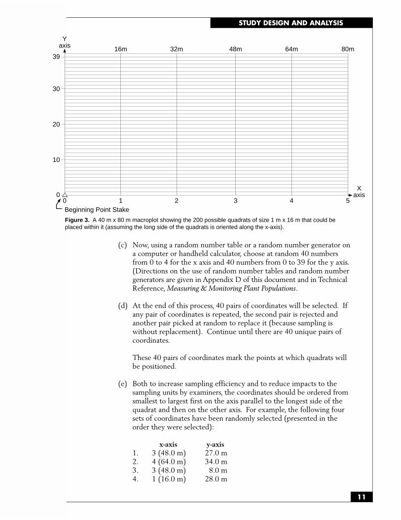
Figure 3. A 40 m x 80 m macroplot showing the 200 possible quadrats of size 1 m x 16 m that could beplaced within it (assuming the long side of the quadrats is oriented along the x-axis).
(c) Now, using a random number table or a random number generator ona computer or handheld calculator, choose at random 40 numbersfrom 0 to 4 for the x axis and 40 numbers from 0 to 39 for the y axis.(Directions on the use of random number tables and random numbergenerators are given in Appendix D of this document and in TechnicalReference, Measuring & Monitoring Plant Populations.
(d) At the end of this process, 40 pairs of coordinates will be selected. Ifany pair of coordinates is repeated, the second pair is rejected andanother pair picked at random to replace it (because sampling iswithout replacement). Continue until there are 40 unique pairs ofcoordinates.
These 40 pairs of coordinates mark the points at which quadrats willbe positioned.
(e) Both to increase sampling efficiency and to reduce impacts to thesampling units by examiners, the coordinates should be ordered fromsmallest to largest first on the axis parallel to the longest side of thequadrat and then on the other axis. For example, the following foursets of coordinates have been randomly selected (presented in theorder they were selected):
x-axis y-axis1. 3 (48.0 m) 27.0 m2. 4 (64.0 m) 34.0 m3. 3 (48.0 m) 8.0 m4. 1 (16.0 m) 28.0 m
STUDY DESIGN AND ANALYSIS
12
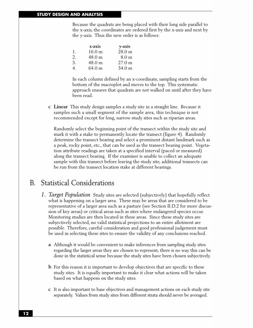
Because the quadrats are being placed with their long side parallel tothe x-axis, the coordinates are ordered first by the x-axis and next bythe y-axis. Thus the new order is as follows:
x-axis y-axis1. 16.0 m 28.0 m2. 48.0 m 8.0 m3. 48.0 m 27.0 m4. 64.0 m 34.0 m
In each column defined by an x-coordinate, sampling starts from thebottom of the macroplot and moves to the top. This systematicapproach ensures that quadrats are not walked on until after they havebeen read.
c Linear This study design samples a study site in a straight line. Because itsamples such a small segment of the sample area, this technique is notrecommended except for long, narrow study sites such as riparian areas.
Randomly select the beginning point of the transect within the study site andmark it with a stake to permanently locate the transect (figure 4). Randomlydetermine the transect bearing and select a prominent distant landmark such asa peak, rocky point, etc., that can be used as the transect bearing point. Vegeta-tion attribute readings are taken at a specified interval (paced or measured)along the transect bearing. If the examiner is unable to collect an adequatesample with this transect before leaving the study site, additional transects canbe run from the transect location stake at different bearings.
B. Statistical Considerations
1. Target Population Study sites are selected (subjectively) that hopefully reflectwhat is happening on a larger area. These may be areas that are considered to berepresentative of a larger area such as a pasture (see Section II.D.2 for more discus-sion of key areas) or critical areas such as sites where endangered species occur.Monitoring studies are then located in these areas. Since these study sites aresubjectively selected, no valid statistical projections to an entire allotment arepossible. Therefore, careful consideration and good professional judgement mustbe used in selecting these sites to ensure the validity of any conclusions reached.
a Although it would be convenient to make inferences from sampling study sitesregarding the larger areas they are chosen to represent, there is no way this can bedone in the statistical sense because the study sites have been chosen subjectively.
b For this reason it is important to develop objectives that are specific to thesestudy sites. It is equally important to make it clear what actions will be takenbased on what happens on the study sites.
c It is also important to base objectives and management actions on each study siteseparately. Values from study sites from different strata should never be averaged.

13
STUDY DESIGN AND ANALYSIS
Figure 4. Study layout for the linear technique.
Transect Bearing Stake
Study Location Stake
End Point of Transect
100-Meter Tape
Midpoint of Transect
Beginning Point of Transect
Quadrats

STUDY DESIGN AND ANALYSIS
14
d From a sampling perspective, it is the study site that constitutes the targetpopulation. The collection of all possible sampling units that could be placed inthe study site is the target population.
2. Random Sampling Critical to valid monitoring study design is that the samplebe drawn randomly from the population of interest. There are several methods ofrandom sampling, many of which are discussed briefly below, but the importantpoint is that all of the statistical analysis techniques available are based on knowingthe probability of selecting a particular sampling unit. If some type of randomselection of sampling units is not incorporated into the study design, the probabil-ity of selection cannot be determined and no statistical inferences can be madeabout the population. (Directions for randomly selecting the location of transectsto be run off of a baseline using random number tables are given in Appendix D).
3. Systematic Sampling Systematic sampling is very common in samplingvegetation. The placement of quadrats along a transect is an example of systematicsampling. To illustrate, let’s say we decide to place ten 1-square-meter quadrats at5-meter (or 5-pace) intervals along a 50-meter transect. We randomly select anumber between 0 and 4 to represent the starting point for the first quadrat alongthe transect and place the remaining 9 quadrats at 5-meter intervals from thisstarting point. Thus, if 10 observations are to be made at 5-meter intervals and therandomly selected number between 0 and 4 is 2, then the first observation is madeat 2 meters and the remaining observations will be placed at 7, 12, 17, 22, 27, 32,37, 42, and 47 meters along the transect. The selection of the starting point forsystematic sampling must be random.
Strictly speaking, systematic sampling is analogous to simple random sampling onlywhen the population being sampled is in random order (for example, see Williams1978). Many natural populations exhibit an aggregated (also called clumped)spatial distribution pattern. This means that nearby units tend to be similar to(correlated with) each other. If, in a systematic sample, the sampling units arespaced far enough apart to reduce this correlation, the systematic sample will tendto furnish a better average and smaller standard error than is the case with arandom sample, because with a completely random sample one is more likely toend up with at least some sampling units close together (see Milne 1959 and thediscussion of sampling an ordered population in Scheaffer et al. 1979).
4. Sampling vs. Nonsampling Errors In any monitoring study, it pays to keepthe error rate as low as possible. Errors can be separated into sampling errors andnonsampling errors.
a Sampling Errors Sampling errors arise from chance variation; they do notresult from “mistakes” such as misidentifying a species. They occur when thesample does not reflect the true population. The magnitude of sampling errorscan be measured.
b Nonsampling Errors Nonsampling errors are “mistakes” that cannot be mea-sured.
15
STUDY DESIGN AND ANALYSIS
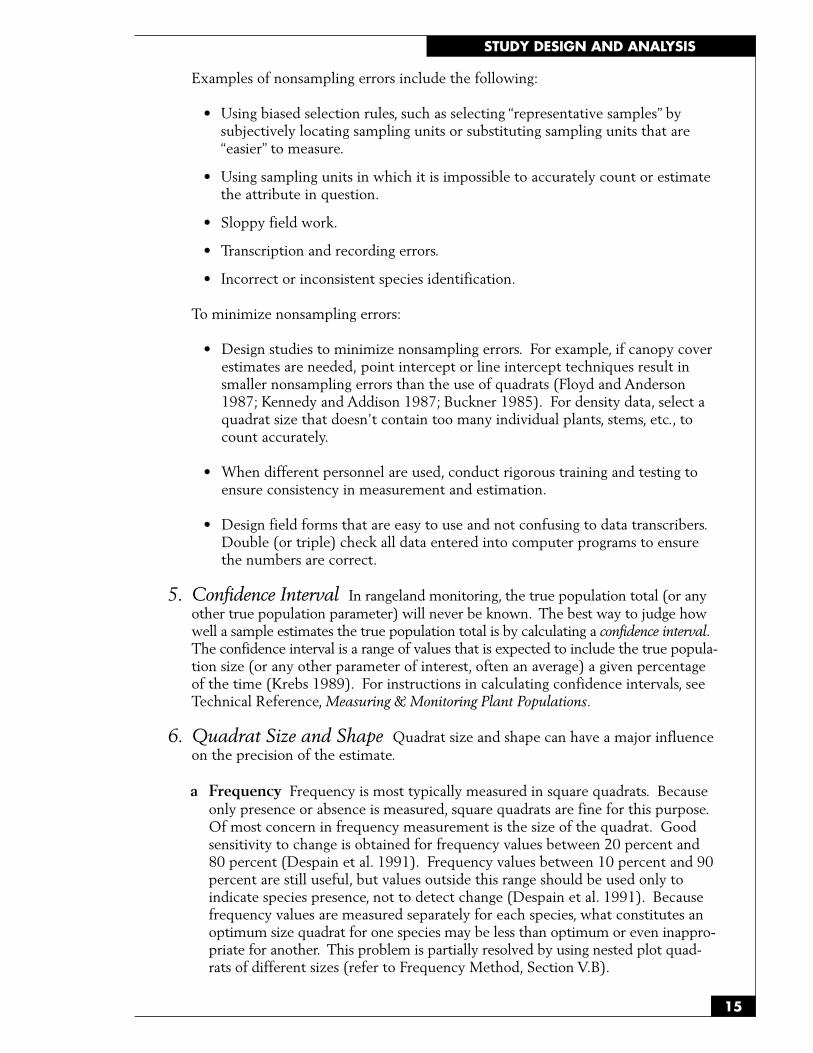
Examples of nonsampling errors include the following:
• Using biased selection rules, such as selecting “representative samples” bysubjectively locating sampling units or substituting sampling units that are“easier” to measure.
• Using sampling units in which it is impossible to accurately count or estimatethe attribute in question.
• Sloppy field work.
• Transcription and recording errors.
• Incorrect or inconsistent species identification.
To minimize nonsampling errors:
• Design studies to minimize nonsampling errors. For example, if canopy coverestimates are needed, point intercept or line intercept techniques result insmaller nonsampling errors than the use of quadrats (Floyd and Anderson1987; Kennedy and Addison 1987; Buckner 1985). For density data, select aquadrat size that doesn’t contain too many individual plants, stems, etc., tocount accurately.
• When different personnel are used, conduct rigorous training and testing toensure consistency in measurement and estimation.
• Design field forms that are easy to use and not confusing to data transcribers.Double (or triple) check all data entered into computer programs to ensurethe numbers are correct.
5. Confidence Interval In rangeland monitoring, the true population total (or anyother true population parameter) will never be known. The best way to judge howwell a sample estimates the true population total is by calculating a confidence interval.The confidence interval is a range of values that is expected to include the true popula-tion size (or any other parameter of interest, often an average) a given percentageof the time (Krebs 1989). For instructions in calculating confidence intervals, seeTechnical Reference, Measuring & Monitoring Plant Populations.
6. Quadrat Size and Shape Quadrat size and shape can have a major influenceon the precision of the estimate.
a Frequency Frequency is most typically measured in square quadrats. Becauseonly presence or absence is measured, square quadrats are fine for this purpose.Of most concern in frequency measurement is the size of the quadrat. Goodsensitivity to change is obtained for frequency values between 20 percent and80 percent (Despain et al. 1991). Frequency values between 10 percent and 90percent are still useful, but values outside this range should be used only toindicate species presence, not to detect change (Despain et al. 1991). Becausefrequency values are measured separately for each species, what constitutes anoptimum size quadrat for one species may be less than optimum or even inappro-priate for another. This problem is partially resolved by using nested plot quad-rats of different sizes (refer to Frequency Method, Section V.B).
STUDY DESIGN AND ANALYSIS
16
b Cover In general, quadrats are not recommended for estimating cover (Floydand Anderson 1987; Kennedy and Addison 1987). Where they are used, thesame types of considerations given below for density apply: long, thin quadratswill likely be better than circular, square, or shorter and wider rectangularquadrats (Krebs 1989). Each situation, however, should be analyzed separately.The amount of area in the quadrat is a concern with cover estimation. Thelarger the area, the more difficult it is to accurately estimate cover.
c Density Long, thin quadrats are better (often very much better) than circles,squares, or shorter and wider quadrats. How narrow the quadrats can be de-pends upon consideration of problems of edge effect, although problems of edgeeffect can be largely eliminated by developing consistent rules for determiningwhether to include or exclude plants that fall directly under quadrat edges.One recommendation is to count plants that are rooted directly under the topand left sides of the quadrat but not those directly rooted under the bottom andright quadrat sides. The amount of area within the quadrat is limited by thedegree of accuracy with which one can count all the plants within each quadrat.
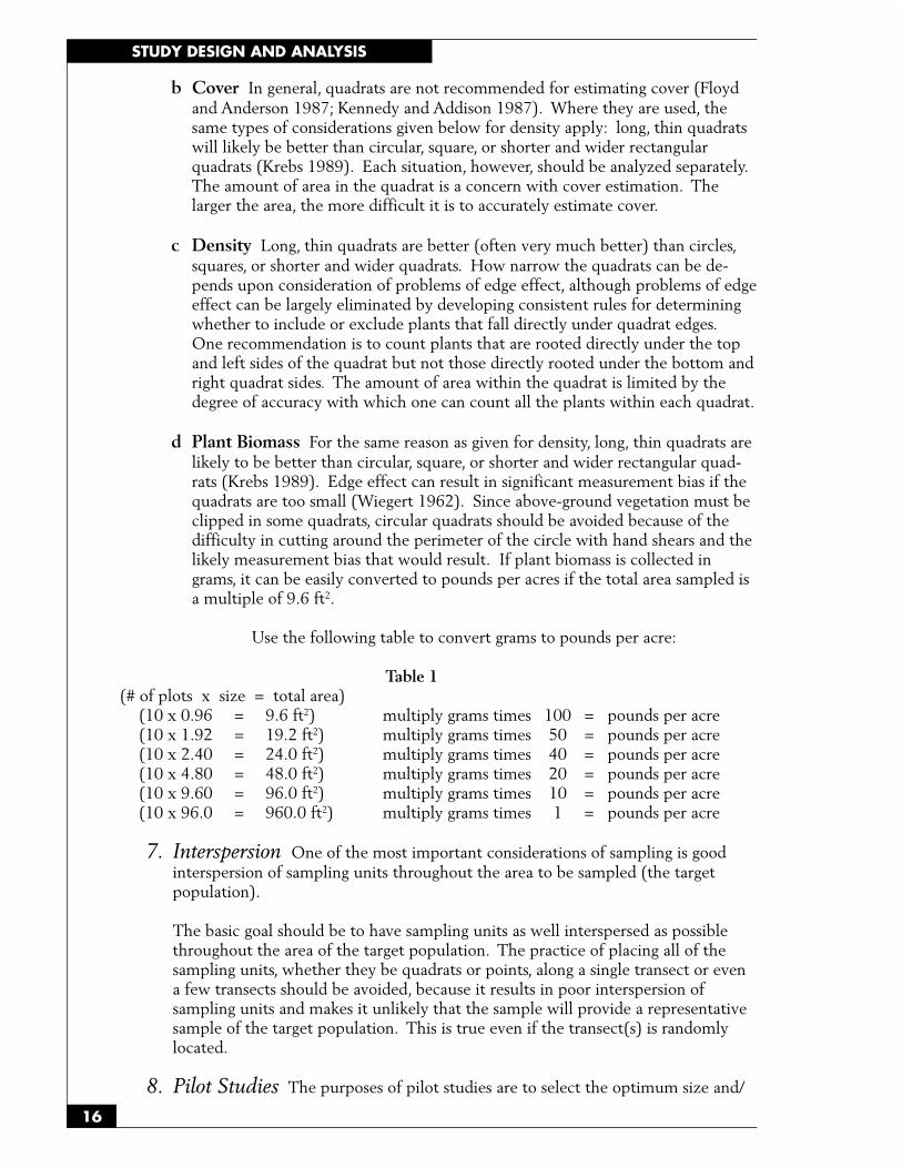
d Plant Biomass For the same reason as given for density, long, thin quadrats arelikely to be better than circular, square, or shorter and wider rectangular quad-rats (Krebs 1989). Edge effect can result in significant measurement bias if thequadrats are too small (Wiegert 1962). Since above-ground vegetation must beclipped in some quadrats, circular quadrats should be avoided because of thedifficulty in cutting around the perimeter of the circle with hand shears and thelikely measurement bias that would result. If plant biomass is collected ingrams, it can be easily converted to pounds per acres if the total area sampled isa multiple of 9.6 ft2.
Use the following table to convert grams to pounds per acre:
Table 1 (# of plots x size = total area)
(10 x 0.96 = 9.6 ft2) multiply grams times 100 = pounds per acre(10 x 1.92 = 19.2 ft2) multiply grams times 50 = pounds per acre(10 x 2.40 = 24.0 ft2) multiply grams times 40 = pounds per acre(10 x 4.80 = 48.0 ft2) multiply grams times 20 = pounds per acre(10 x 9.60 = 96.0 ft2) multiply grams times 10 = pounds per acre(10 x 96.0 = 960.0 ft2) multiply grams times 1 = pounds per acre
7. Interspersion One of the most important considerations of sampling is goodinterspersion of sampling units throughout the area to be sampled (the targetpopulation).
The basic goal should be to have sampling units as well interspersed as possiblethroughout the area of the target population. The practice of placing all of thesampling units, whether they be quadrats or points, along a single transect or evena few transects should be avoided, because it results in poor interspersion ofsampling units and makes it unlikely that the sample will provide a representativesample of the target population. This is true even if the transect(s) is randomlylocated.
8. Pilot Studies The purposes of pilot studies are to select the optimum size and/
17
STUDY DESIGN AND ANALYSIS
or shape of the sampling unit for the study and to determine how much variabilityexists in the population being sampled. The latter information is necessary todetermine the sample size necessary to meet specific management and monitoringobjectives.
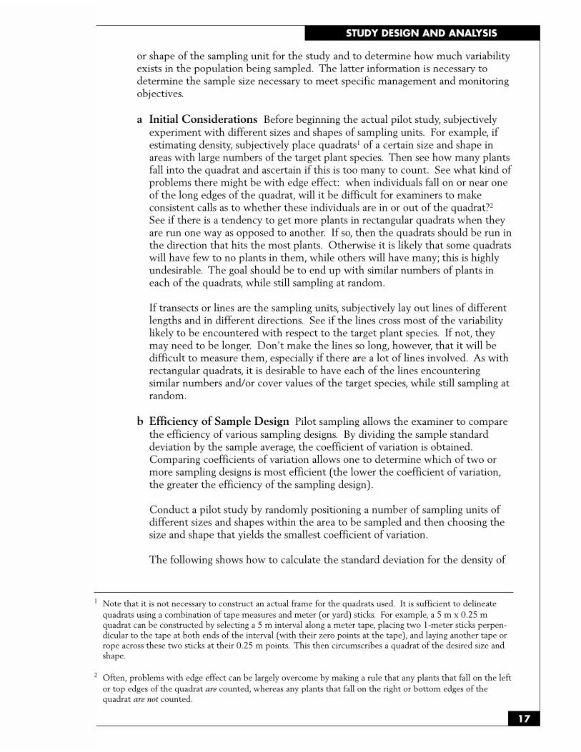
a Initial Considerations Before beginning the actual pilot study, subjectivelyexperiment with different sizes and shapes of sampling units. For example, ifestimating density, subjectively place quadrats1 of a certain size and shape inareas with large numbers of the target plant species. Then see how many plantsfall into the quadrat and ascertain if this is too many to count. See what kind ofproblems there might be with edge effect: when individuals fall on or near oneof the long edges of the quadrat, will it be difficult for examiners to makeconsistent calls as to whether these individuals are in or out of the quadrat?2
See if there is a tendency to get more plants in rectangular quadrats when theyare run one way as opposed to another. If so, then the quadrats should be run inthe direction that hits the most plants. Otherwise it is likely that some quadratswill have few to no plants in them, while others will have many; this is highlyundesirable. The goal should be to end up with similar numbers of plants ineach of the quadrats, while still sampling at random.
If transects or lines are the sampling units, subjectively lay out lines of differentlengths and in different directions. See if the lines cross most of the variabilitylikely to be encountered with respect to the target plant species. If not, theymay need to be longer. Don’t make the lines so long, however, that it will bedifficult to measure them, especially if there are a lot of lines involved. As withrectangular quadrats, it is desirable to have each of the lines encounteringsimilar numbers and/or cover values of the target species, while still sampling atrandom.
b Efficiency of Sample Design Pilot sampling allows the examiner to comparethe efficiency of various sampling designs. By dividing the sample standarddeviation by the sample average, the coefficient of variation is obtained.Comparing coefficients of variation allows one to determine which of two ormore sampling designs is most efficient (the lower the coefficient of variation,the greater the efficiency of the sampling design).
Conduct a pilot study by randomly positioning a number of sampling units ofdifferent sizes and shapes within the area to be sampled and then choosing thesize and shape that yields the smallest coefficient of variation.
The following shows how to calculate the standard deviation for the density of
1 Note that it is not necessary to construct an actual frame for the quadrats used. It is sufficient to delineatequadrats using a combination of tape measures and meter (or yard) sticks. For example, a 5 m x 0.25 mquadrat can be constructed by selecting a 5 m interval along a meter tape, placing two 1-meter sticks perpen-dicular to the tape at both ends of the interval (with their zero points at the tape), and laying another tape orrope across these two sticks at their 0.25 m points. This then circumscribes a quadrat of the desired size andshape.
2 Often, problems with edge effect can be largely overcome by making a rule that any plants that fall on the leftor top edges of the quadrat are counted, whereas any plants that fall on the right or bottom edges of thequadrat are not counted.
STUDY DESIGN AND ANALYSIS
18
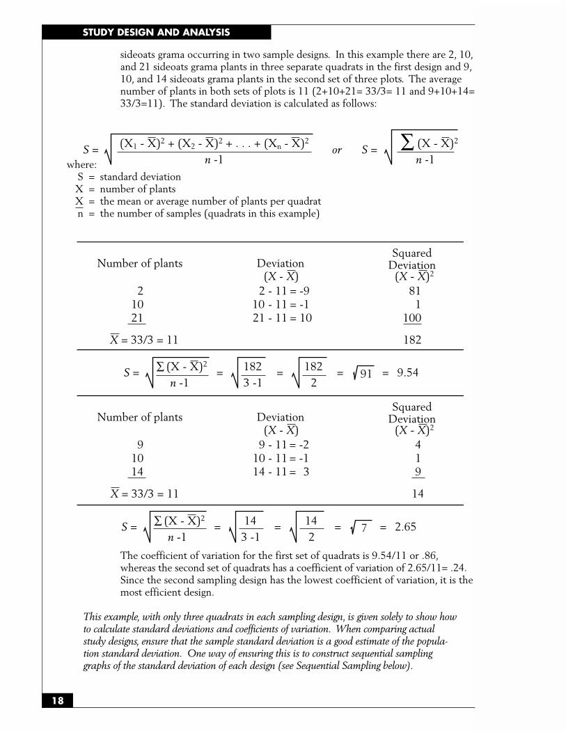
sideoats grama occurring in two sample designs. In this example there are 2, 10,and 21 sideoats grama plants in three separate quadrats in the first design and 9,10, and 14 sideoats grama plants in the second set of three plots. The averagenumber of plants in both sets of plots is 11 (2+10+21= 33/3= 11 and 9+10+14=33/3=11). The standard deviation is calculated as follows:
where:S = standard deviationX = number of plantsX = the mean or average number of plants per quadratn = the number of samples (quadrats in this example)
The coefficient of variation for the first set of quadrats is 9.54/11 or .86,whereas the second set of quadrats has a coefficient of variation of 2.65/11= .24.Since the second sampling design has the lowest coefficient of variation, it is themost efficient design.
This example, with only three quadrats in each sampling design, is given solely to show howto calculate standard deviations and coefficients of variation. When comparing actualstudy designs, ensure that the sample standard deviation is a good estimate of the popula-tion standard deviation. One way of ensuring this is to construct sequential samplinggraphs of the standard deviation of each design (see Sequential Sampling below).
(X - X)2
n -1S = = = = = 9.54
Number of plants
21021
2 - 1110 - 1121 - 11
= -9= -1= 10
(X - X)
X = 33/3 = 11 182
DeviationSquared
Deviation
1823 -1
18291
2
(X - X)2
n -1S = = = = = 2.6514
3 -114
72
811
100
(X - X)2
Number of plants
91014
9 - 1110 - 1114 - 11
= -2= -1= 3
(X - X)
X = 33/3 = 11 14
DeviationSquared
Deviation
419
(X - X)2
(X1 - X)2 + (X2 - X)2 + . . . + (Xn - X)2 (X - X)2
n -1S = S =or
n -1

19
STUDY DESIGN AND ANALYSIS
Wiegert (1962), summarized in Krebs (1989:67-72), gives a quantitativemethod for determining optimal quadrat size and/or shape. The method con-siders the costs involved in locating and measuring quadrats and the standarddeviation (or its square, the variance) that results from samples of that size andshape. Refer to Krebs’ book for details (and an example).
c Sequential Sampling The estimate of the standard deviation derived throughpilot sampling is one of the values used to calculate sample size, whether oneuses the formulas given in Technical Reference, Measuring & Monitoring PlantPopulations, or uses a computer program.
When conducting the pilot sampling, employ sequential sampling. Sequentialsampling helps determine whether the examiner has taken a large enough pilotsample to properly evaluate different sampling designs and/or to use the stan-dard deviation from the pilot sample to calculate sample size. The process isaccomplished as follows:
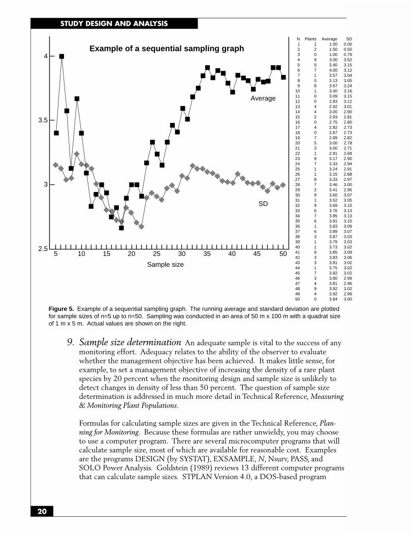
Gather pilot sampling data using some arbitrarily selected sample size. Calculatethe average and standard deviation for the first two quadrats, calculate it againafter putting in the next quadrat value, and continue these iterative calculationsafter the addition of each quadrat value to the sample. This will generate arunning average and standard deviation. Look at the four columns of numbers onthe right of Figure 5 for an example of how to carry out this procedure.
Plot on graph paper (or use a computer program) the sample size versus theaverage and standard deviation. Look for curves smoothing out. In the exampleshown in Figure 5, the curves smooth out after n = 30-35. The decision to stopsampling is a subjective one. There are no hard and fast rules.
A computer is valuable for creating sequential sampling graphs. Spreadsheetprograms such as Lotus 1-2-3 allow for entering the data in a form that can laterbe analyzed while at the same time creating a sequential sampling graph of therunning average and standard deviation. This further allows the examiner tolook at several random sequences of the data before deciding on the number ofsampling units to measure.
Use the sequential sampling method to determine what sample size not to use(don’t use a sample size below the point where the running average andstandard deviation have not stabilized). Plug the final average and standarddeviation information into the appropriate sample size equation to actuallydetermine the necessary sample size.
STUDY DESIGN AND ANALYSIS
20
Figure 5. Example of a sequential sampling graph. The running average and standard deviation are plottedfor sample sizes of n=5 up to n=50. Sampling was conducted in an area of 50 m x 100 m with a quadrat sizeof 1 m x 5 m. Actual values are shown on the right.
Sample size
SD
50454035302520151052.5
3
Average
N123456789
1011121314151617181920212223242526272829303132333435363738394041424344454647484950
Plants12095710810044204075319711872919676163119331734940
Average1.001.501.003.003.404.003.573.133.673.403.092.832.923.002.932.752.822.672.893.003.002.913.173.333.243.153.333.463.413.603.523.693.763.853.913.833.893.873.793.733.853.833.813.753.823.803.813.923.923.84
SD0.000.500.793.523.153.123.043.053.243.163.153.123.012.902.812.802.732.732.822.782.712.682.902.942.912.882.973.002.953.073.053.153.133.133.103.093.073.033.033.023.093.063.023.023.022.992.963.022.993.00
Example of a sequential sampling graph
3.5
4
9. Sample size determination An adequate sample is vital to the success of anymonitoring effort. Adequacy relates to the ability of the observer to evaluatewhether the management objective has been achieved. It makes little sense, forexample, to set a management objective of increasing the density of a rare plantspecies by 20 percent when the monitoring design and sample size is unlikely todetect changes in density of less than 50 percent. The question of sample sizedetermination is addressed in much more detail in Technical Reference, Measuring& Monitoring Plant Populations.
Formulas for calculating sample sizes are given in the Technical Reference, Plan-ning for Monitoring. Because these formulas are rather unwieldy, you may chooseto use a computer program. There are several microcomputer programs that willcalculate sample size, most of which are available for reasonable cost. Examplesare the programs DESIGN (by SYSTAT), EXSAMPLE, N, Nsurv, PASS, andSOLO Power Analysis. Goldstein (1989) reviews 13 different computer programsthat can calculate sample sizes. STPLAN Version 4.0, a DOS-based program
21
STUDY DESIGN AND ANALYSIS
developed by Brown et al. (1993), is available as freeware from the followingInternet ftp (file transfer protocol) site: odin.mda.uth.tmc.edu. Documentation isincluded with the program. The program calculates sample sizes needed for all ofthe types of significance testing but does not calculate those required for estimat-ing a single population average, total, or proportion. PC-SIZE: CONSULTANT is ashareware program that will calculate sample sizes for estimating an average (butnot a proportion) and for all the types of significance tests. It was developed in1990 by Gerard E. Dallal, who also developed the commercial program DESIGNdiscussed above. PC-SIZE: CONSULTANT appears to contain all of the algo-rithms included in DESIGN but at a fraction of the cost (the author asks for a feeof $15.00 if the user finds the program to be useful). The program is available viathe World Wide Web at the following address:
http://www.coast.net/SimTel/SimTel/
Once at the homepage, change to the directory msdos/statstic/ and download thefile st-size.zip. Unzip the file using the shareware program PKUNZIP. Executablefiles and documentation are included.
Alternatively, tables can be used to calculate sample size. For detecting change inaverages, proportions, or totals between two time periods, the tables found inCohen (1988) are highly recommended.
10. Graphical Display of Data The use of graphs, both to initially explore thequality of the monitoring data collected and to display the results of the dataanalysis, is important to designing and implementing monitoring studies. SeeTechnical Reference, Measuring & Monitoring Plant Populations, for descriptions ofthese graphs, along with examples.
a Graphs to Examine Study Data Prior to Analysis The best of these graphsplot each data point. These graphs can help determine whether the data meetthe assumptions of parametric statistics, or whether the data set contains outliers(data with values much lower or much higher than most of the rest of the data—asmight occur if one made a mistake in measuring or recording). Normal probabil-ity plots and box plots are two of the most useful types for this purpose. Graphscan also assist in determining appropriate quadrat size. For more information, seeTechnical Reference, Measuring & Monitoring Plant Populations.
b Graphs to Display the Results of Data Analysis Rather than displayingeach data point, these graphs display summary statistics (i.e., averages, totals, orproportions). When these summary statistics are graphed, error bars must beused to display the precision of estimates. Because it is the true parameter(average, median, total, or proportion) that is of interest, confidence intervalsshould be used as error bars. Types of graphs include:
• Bar charts with confidence intervals.
• Graphs of summary statistics plotted as points, with error bars.
• Box plots with “notches” for error bars.

STUDY DESIGN AND ANALYSIS
22
C. Other Important Considerations
1. Sampling All Species Although the key species concept is important in ana-lyzing and evaluating management actions, other species should also be consideredfor sampling. Whenever possible, all species should be sampled, especially on theinitial sampling. It is also important to record sampling data by individual speciesrather than by genera, form class, or other grouping. These data can be lumpedlater during the analysis if appropriate. Both of these approaches will providegreater flexibility in data analysis if objectives or key species change in the future.
2. Plant Species Identification The plant species must be properly identified inorder for the data to be useful in grazing allotment, wildlife habitat area, herdmanagement area, watershed area, or other designated management area evalua-tions. In some cases, it may be helpful to include pressed plant specimens, photo-graphs, or other aids used for species identification in the study file. If data arecollected prior to positive species identification, examiners should collect plantspecimens for later verification.
3. Training The purpose of training is to provide resource specialists with thenecessary skills for implementing studies and collecting reliable, unbiased, andconsistent data. Examiners should understand data collection, documentation,analysis, interpretation, and evaluation procedures, including the need foruniformity, accuracy, and reliable monitoring data.
Training should occur in the field by qualified personnel to ensure that examiners arefamiliar with the equipment and supplies and that detailed procedural instructionsare thoroughly demonstrated and understood.
As a follow-up to the training, data collected should be examined early in thestudy effort to ensure that the data are properly collected and recorded.
Periodic review and/or recalibration during the field season may be necessary formaintaining consistency among examiners because of progressive phenologicalchanges. Review and recalibration during each field season are especially importantwhere data collection methods require estimates rather than direct measurements.

23
ATTRIBUTES
IV. ATTRIBUTES
The following is a matrix of monitoring techniques and vegetation attributes that are de-scribed in this reference. The X indicates that this is the primary attribute that the tech-nique collects. Some techniques have the capability of collecting other attributes; the •indicates the secondary attribute that can be collected or calculated.
Method Frequency Cover Density Production Structure Composition
Frequency X •
Dry-weight-Rank • • X3
Daubenmire • X •
Line Intercept X •
Step Point X •
Point Intercept X •
Density X •
Double WeightSampling X •
Harvest X •
ComparativeYield X •
Cover Board X X
Robel Pole • X
A. Frequency
1. Description Frequency is one of the easiest and fastest methods available formonitoring vegetation. It describes the abundance and distribution of species andis useful to detect changes in a plant community over time.
Frequency has been used to determine rangeland condition but only limited workhas been done in most communities. This makes the interpretation difficult. Theliterature has discussed the relationship between density and frequency but thisrelationship is only consistent with randomly distributed plants (Greig-Smith 1983).
3 Species composition is calculated using production data. Frequency data should not be used to calculatespecies composition.

ATTRIBUTES
24
Frequency is the number of times a species is present in a given number of samplingunits. It is usually expressed as a percentage.
2. Advantages and Limitations
a Frequency is highly influenced by the size and shape of the quadrats used.Quadrats or nested quadrats are the most common measurement used; how-ever, point sampling and step point methods have also been used to estimatefrequency. The size and shape of a quadrat needed to adequately determinefrequency depends on the distribution, number, and size of the plant species.
b To determine change, the frequency of a species must generally be at least 20%and no greater than 80%. Frequency comparisons must be made with quadratsof the same size and shape. While change can be detected with frequency, theextent to which the vegetation community has changed cannot be determined.
c High repeatability is obtainable.
d Frequency is highly sensitive to changes resulting from seedling establishment.Seedlings present one year may not be persistent the following year. Thissituation is problematic if data is collected only every few years. It is less of aproblem if seedlings are recorded separately.
e Frequency is also very sensitive to changes in pattern of distribution in thesampled area.
f Rooted frequency data is less sensitive to fluctuations in climatic and bioticinfluences.
g Interpretation of changes in frequency is difficult because of the inability todetermine the vegetation attribute that changed. Frequency cannot tell whichof three parameters has changed: canopy cover, density, or pattern of distribution.
3. Appropriate Use of Frequency for Rangeland Monitoring If the pri-mary reason for collecting frequency data is to demonstrate that a change invegetation has occurred, then on most sites the frequency method is capable ofaccomplishing the task with statistical evidence more rapidly and at less cost thanany other method that is currently available (Hironaka 1985).
Frequency should not be the only data collected if time and money are available.Additional information on ground cover, plant cover, and other vegetation and sitedata would contribute to a better understanding of the changes that have occurred(Hironaka 1985).
West (1985) noted the following limitations: “Because of the greater risk ofmisjudging a downward than upward trend, frequency may provide the easiestearly warning of undesirable changes in key or indicator species. However, becausefrequency data are so dependent on quadrat size and sensitive to non-randomdispersion patterns that prevail on rangelands, managers are fooling themselves ifthey calculate percentage composition from frequency data and try to comparedifferent sites at the same time or the same site over time in terms of total species

25
ATTRIBUTES
composition. This is because the numbers derived for frequency sampling areunique to the choice of sample size, shape, number, and placement. For variablesof cover and weight, accuracy is mostly what is affected by these choices and thevariable can be conceived independently of the sampling protocol.”
B. Cover
1. Description Cover is an important vegetation and hydrologic characteristic. Itcan be used in various ways to determine the contribution of each species to aplant community. Cover is also important in determining the proper hydrologicfunction of a site. This characteristic is very sensitive to biotic and edaphic forces.For watershed stability, some have tried to use a standard soil cover, but researchhas shown each edaphic site has its own potential cover.
Cover is generally referred to as the percentage of ground surface covered byvegetation. However, numerous definitions exist. It can be expressed in absoluteterms (square meters/hectares) but is most often expressed as a percentage. Theobjective being measured will determine the definition and type of cover measured.
a Vegetation cover is the total cover of vegetation on a site.
b Foliar cover is the area of ground covered by the vertical projection of the aerialportions of the plants. Small openings in the canopy and intraspecific overlapare excluded (Figure 6).
c Canopy cover is the area of ground covered by the vertical projection of theoutermost perimeter of the natural spread of foliage of plants. Small openingswithin the canopy are included. It may exceed 100% (Figure 7).
d Basal cover is the area of ground surface occupied by the basal portion of theplants.
e Ground cover is the cover of plants, litter, rocks, and gravel on a site.
Figure 6. Foliar cover. Figure 7. Canopy cover.

ATTRIBUTES
26
2. Advantages and Limitations
a Ground cover is most often used to determine the watershed stability of thesite, but comparisons between sites are difficult to interpret because of thedifferent potentials associated with each ecological site.
b Vegetation cover is a component of ground cover and is often sensitive toclimatic fluctuations that can cause errors in interpretation. Canopy cover andfoliar cover are components of vegetation cover and are the most sensitive toclimatic and biotic factors. This is particularly true with herbaceous vegetation.
c Overlapping canopy cover often creates problems, particularly in mixed com-munities. If species composition is to be determined, the canopy of each spe-cies is counted regardless of any overlap with other species. If watershedcharacteristics are the objective, only the uppermost canopy is generallycounted.
d For trend comparisons in herbaceous plant communities, basal cover is generallyconsidered to be the most stable. It does not vary as much due to climaticfluctuations or current-year grazing.
C. Density
1. Description Density has been used to describe characteristics of plant communi-ties. However, comparisons can only be based on similar life-form and size. This iswhy density is rarely used as a measurement by itself when describing plant com-munities. For example, the importance of a particular species to a community isvery different if there are 1,000 annual plants per acre versus 1,000 shrubs peracre. It should be pointed out that density was synonymous with cover in theearlier literature.
Density is basically the number of individuals per unit area. The term refers to thecloseness of individual plants to one another.
2. Advantages and Limitations
a Density is useful in monitoring threatened and endangered species or otherspecial status plants because it samples the number of individuals per unit area.
b Density is useful when comparing similar life-forms (annuals to annuals, shrubsto shrubs) that are approximately the same size. For trend measurements, thisparameter is used to determine if the number of individuals of a specific speciesis increasing or decreasing.
c The problem with using density is being able to identify individuals and com-paring individuals of different sizes. It is often hard to identify individuals ofplants that are capable of vegetative reproduction (e.g., rhizomatous plants likewestern wheatgrass or Gambles oak). Comparisons of bunchgrass plants torhizomatous plants are often meaningless because of these problems. Similarproblems occur when looking at the density of shrubs of different growth forms

27
ATTRIBUTES
or comparing seedlings to mature plants. Density on rhizomatous or stolonifer-ous plants is determined by counting the number of stems instead of the num-ber of individuals. Seedling density is directly related to environmental condi-tions and can often be interpreted erroneously as a positive or negative trendmeasurement. Because of these limitations, density has generally been usedwith shrubs and not herbaceous vegetation. Seedlings and mature plants shouldbe recorded separately.
If the individuals can be identified, density measurements are repeatable overtime because there is small observer error. The type of vegetation and distribu-tion will dictate the technique used to obtain the density measurements. Inhomogenous plant communities, which are rare, square quadrats have beenrecommended, while heterogenous communities should be sampled withrectangular or line strip quadrats. Plotless methods have also been developedfor widely dispersed plants.
D. Production
1. Description Many believe that the relative production of different species in aplant community is the best measure of these species’ roles in the ecosystem.
The terminology associated with vegetation biomass is normally related toproduction.
a Gross primary production is the total amount of organic material produced,both above ground and below ground.
b Biomass is the total weight of living organisms in the ecosystem, includingplants and animals.
c Standing crop is the amount of plant biomass present above ground at any givenpoint.
d Peak standing crop is the greatest amount of plant biomass above groundpresent during a given year.
e Total forage is the total herbaceous and woody palatable plant biomass availableto herbivores.
f Allocated forage is the difference of desired amount of residual material subtractedfrom the total forage.
g Browse is the portion of woody plant biomass accessible to herbivores.
2. Advantages and Limitations
a Biomass and gross primary production are rarely used in rangeland trend studiesbecause it is impractical to obtain the measurements below ground. In addition,the animal portion of biomass is rarely obtainable.
ATTRIBUTES
28
b Standing crop and peak standing crop are the measurements most often used intrend studies. Peak standing crop is generally measured at the end of the growingseason. However, different species reach their peak standing crop at differenttimes. This can be a significant problem in mixed plant communities.
c Often, the greater the diversity of plant species or growth patterns, the largerthe error if only one measurement is made.
d Other problems associated with the use of plant biomass are that fluctuations inclimate and biotic influences can alter the estimates. When dealing with largeungulates, exclosures are generally required to measure this parameter. Severalauthors have suggested that approximately 25% of the peak standing crop isconsumed by insects or trampled; this is rarely discussed in most trend studies.
e Collecting production data also tends to be time and labor intensive. Cover andfrequency have been used to estimate plant biomass in some species.
E. Structure
1. Description Structure of vegetation primarily looks at how the vegetation isarranged in a three-dimensional space. The primary use for structure measure-ments is to help evaluate a vegetation community’s value in providing habitat forassociated wildlife species.
Vegetation is measured in layers on vertical planes. Measurements generally lookat the vertical distribution by either estimating the cover of each layer or bymeasuring the height of the vegetation.
2. Advantages and Limitations Structure data provide information that isuseful in describing the suitability of the sites for screening and escape cover,which are important for wildlife. Methods used to collect these data are quick,allowing for numerous samples to be obtained over relatively large areas. Methodsthat use visual obstruction techniques to evaluate vegetation height have littleobserver bias. Those techniques that estimate cover require more training toreduce observer bias. Structure is rarely used by itself when describing trend.
F. Composition
1. Description Composition is a calculated attribute rather than one that is directlycollected in the field. It is the proportion of various plant species in relation to thetotal of a given area. It may be expressed in terms of relative cover, relative density,relative weight, etc.
Composition has been used extensively to describe ecological sites and to evaluaterangeland condition.
To calculate composition, the individual value (weight, density, percent cover) fora species or group of species is divided by the total value of the entire population.
29
ATTRIBUTES
2. Advantages and Limitations
a Quadrats, point sampling, and step point methods can all be used to calculatecomposition.
b The repeatability of determining composition depends on the attribute col-lected and the method used.
c Sensitivity to change is dependent on the attribute used to calculate composition.For instance, if plant biomass is used to calculate composition, the values canvary with climatic conditions and the timing of climatic events (precipitation,frost-free period, etc.). Composition based on basal cover, on the other hand,would be relatively stable.
d Composition allows the comparison of vegetation communities at variouslocations within the same ecological sites.

ATTRIBUTES
30
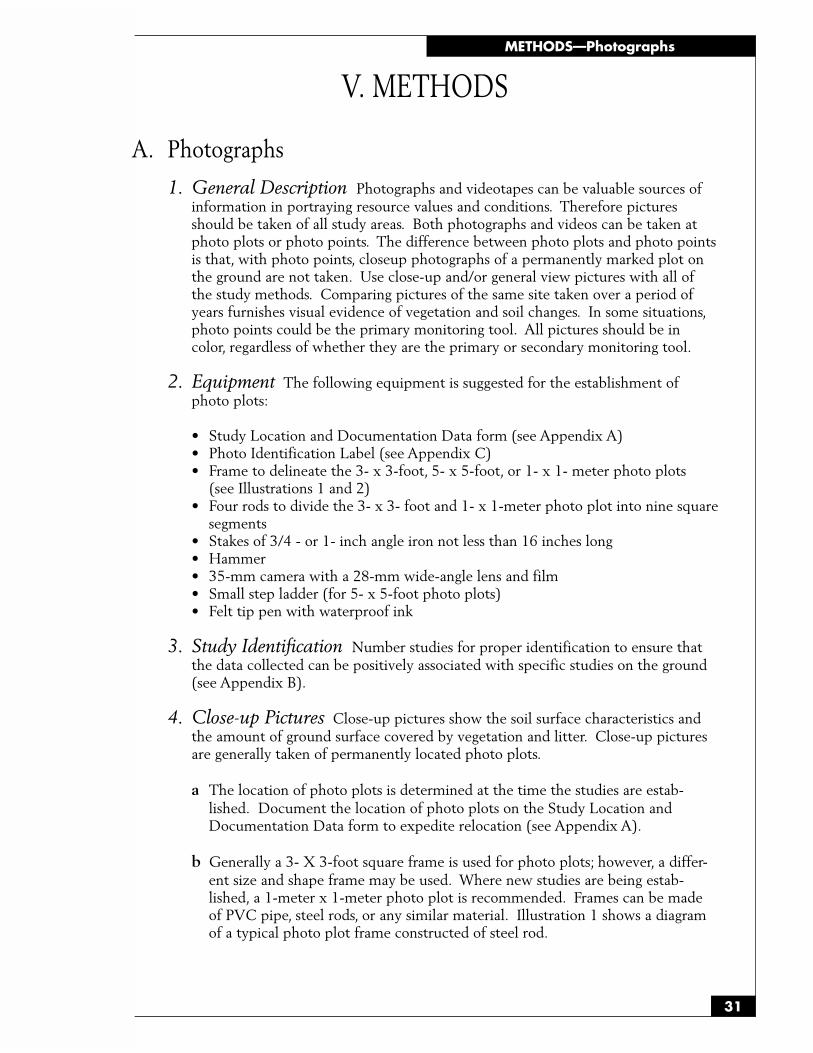
31
METHODS—Photographs
V. METHODS
A. Photographs
1. General Description Photographs and videotapes can be valuable sources ofinformation in portraying resource values and conditions. Therefore picturesshould be taken of all study areas. Both photographs and videos can be taken atphoto plots or photo points. The difference between photo plots and photo pointsis that, with photo points, closeup photographs of a permanently marked plot onthe ground are not taken. Use close-up and/or general view pictures with all ofthe study methods. Comparing pictures of the same site taken over a period ofyears furnishes visual evidence of vegetation and soil changes. In some situations,photo points could be the primary monitoring tool. All pictures should be incolor, regardless of whether they are the primary or secondary monitoring tool.
2. Equipment The following equipment is suggested for the establishment ofphoto plots:
• Study Location and Documentation Data form (see Appendix A)• Photo Identification Label (see Appendix C)• Frame to delineate the 3- x 3-foot, 5- x 5-foot, or 1- x 1- meter photo plots
(see Illustrations 1 and 2)• Four rods to divide the 3- x 3- foot and 1- x 1-meter photo plot into nine square
segments• Stakes of 3/4 - or 1- inch angle iron not less than 16 inches long• Hammer• 35-mm camera with a 28-mm wide-angle lens and film• Small step ladder (for 5- x 5-foot photo plots)• Felt tip pen with waterproof ink
3. Study Identification Number studies for proper identification to ensure thatthe data collected can be positively associated with specific studies on the ground(see Appendix B).
4. Close-up Pictures Close-up pictures show the soil surface characteristics andthe amount of ground surface covered by vegetation and litter. Close-up picturesare generally taken of permanently located photo plots.
a The location of photo plots is determined at the time the studies are estab-lished. Document the location of photo plots on the Study Location andDocumentation Data form to expedite relocation (see Appendix A).
b Generally a 3- X 3-foot square frame is used for photo plots; however, a differ-ent size and shape frame may be used. Where new studies are being estab-lished, a 1-meter x 1-meter photo plot is recommended. Frames can be madeof PVC pipe, steel rods, or any similar material. Illustration 1 shows a diagramof a typical photo plot frame constructed of steel rod.
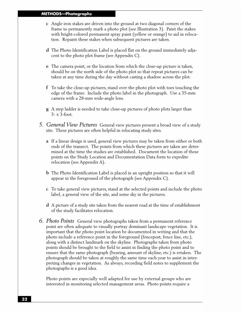
METHODS—Photographs
32
c Angle iron stakes are driven into the ground at two diagonal corners of theframe to permanently mark a photo plot (see Illustration 3). Paint the stakeswith bright-colored permanent spray paint (yellow or orange) to aid in reloca-tion. Repaint these stakes when subsequent pictures are taken.
d The Photo Identification Label is placed flat on the ground immediately adja-cent to the photo plot frame (see Appendix C).
e The camera point, or the location from which the close-up picture is taken,should be on the north side of the photo plot so that repeat pictures can betaken at any time during the day without casting a shadow across the plot.
f To take the close-up pictures, stand over the photo plot with toes touching theedge of the frame. Include the photo label in the photograph. Use a 35-mmcamera with a 28-mm wide-angle lens.
g A step ladder is needed to take close-up pictures of photo plots larger than3- x 3-foot.
5. General View Pictures General view pictures present a broad view of a studysite. These pictures are often helpful in relocating study sites.
a If a linear design is used, general view pictures may be taken from either or bothends of the transect. The points from which these pictures are taken are deter-mined at the time the studies are established. Document the location of thesepoints on the Study Location and Documentation Data form to expediterelocation (see Appendix A).
b The Photo Identification Label is placed in an upright position so that it willappear in the foreground of the photograph (see Appendix C).
c To take general view pictures, stand at the selected points and include the photolabel, a general view of the site, and some sky in the pictures.
d A picture of a study site taken from the nearest road at the time of establishmentof the study facilitates relocation.
6. Photo Points General view photographs taken from a permanent referencepoint are often adequate to visually portray dominant landscape vegetation. It isimportant that the photo point location be documented in writing and that thephoto include a reference point in the foreground (fencepost, fence line, etc.),along with a distinct landmark on the skyline. Photographs taken from photopoints should be brought to the field to assist in finding the photo point and toensure that the same photograph (bearing, amount of skyline, etc.) is retaken. Thephotograph should be taken at roughly the same time each year to assist in inter-preting changes in vegetation. As always, recording field notes to supplement thephotographs is a good idea.
Photo points are especially well adapted for use by external groups who areinterested in monitoring selected management areas. Photo points require a
33
METHODS—Photographs
camera, film, and local knowledge of photo point location; given these, they areeasy to set up and retake. Agencies can encourage participation by external groupsor permittees by providing the photographer with film and development. Doubleprints allow the agency and photographer to keep copies of photographs for theirfiles. Negatives should generally be kept and filed at the agency office.
7. Video Images Video cameras, i.e., camcorders, are now available and are able torecord multiple images of landscapes for monitoring. While video images providenew ways to record landscape images, limitations in their use should also beconsidered. Video tapes, especially the quality of the image, may begin to deterio-rate within 5 years. These images can be protected by conversion to digital com-puter images (expensive) or rerecording the original tape onto a new blank tape.
Comparing repeat video images is difficult, especially if the same landscape se-quences are not repeated in the same way on subsequent video recordings. Videocameras are also more susceptible to dust and heat damage and cost considerablymore than 35-mm cameras. Advantages and disadvantages of video camerasshould be carefully considered prior to implementing a video monitoring system.
8. Repeat Pictures When repeat pictures are taken, follow the same process usedin taking the initial pictures. Include the same area and landmarks in the repeatgeneral view pictures that were included in the initial pictures. Take repeat picturesat approximately the same time of year as the original pictures.
9. General Observations General observations concerning the sites on whichphotographs are taken can be important in interpreting the photos. Such factors asrodent use, insect infestation, animal concentration, fire, vandalism, and other siteuses can have considerable impact on vegetation and soil resources. This informa-tion can be recorded on note paper or on study method forms themselves if thephotographs are taken while collecting other monitoring data.
10. References
USDI, Bureau of Land Management. 1985. Rangeland monitoring - Trendstudies TR4400-4.
USDA, Forest Service. 1994. Rangeland Analysis and Management TrainingGuide, Rocky Mountain Region USDA Forest Service Denver, CO.
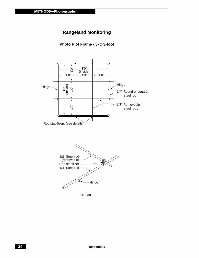
METHODS—Photographs
34 Illustration 1
HingeHinge
1/4" Round or squaresteel rod
1/8" Removablesteel rods
Rod stabilizers (see detail)
1/8" Steel rod(removable)
Rod stabilizer1/4" Steel rod
Hinge
DETAIL
Photo Plot Frame - 3- x 3-foot
Rangeland Monitoring
3'0"(inside)
1'0" 1'0"1'0"1'
0"1'
0"
3'0"
(insi
de)
1'0"

35
METHODS—Photographs
Illustration 2
18" DETAIL
20"
2"
Set screws
Telescoping legs(see detail)
3/4 Light tubingHinge
Hinge
Photo Plot Frame—5- x 5-foot
Rangeland Monitoring
5'0"(inside)5'0"
(inside)

METHODS—Photographs
36 Illustration 3
Paint the stakes with bright-colored permanent spray paint(yellow or orange) to aid in relocation. Repaint these stakeswhen subsequent photographs are taken.
(3- x 3-foot, 5- x 5-foot, or 1- x 1-meter outline)
Camera Point—Permanent Stake(locate on north side of plot)
angle ironstake
angle ironstake
Rangeland Monitoring
Permanent Photo Plot Location

37
METHODS—Frequency
B. Frequency Methods - Pace Frequency, QuadratFrequency, and Nested Frequency Methods
1. General Description All three methods consist of observing quadrats alongtransects, with quadrats systematically located at specified intervals along eachtransect. The only differences in these technique are the size and configuration ofthe quadrat frames and the layout of the transect. The following vegetation at-tributes are monitored with this method:
• Frequency
• Basal cover and general cover categories (including litter)
• Reproduction of key species (if seedling data are collected)
It is important to establish a photo plot (see Section V.A) and take both close-upand general view photographs. This allows the portrayal of resource values andconditions and furnishes visual evidence of vegetation and soil changes over time.
2. Areas of Use This method is applicable to a wide variety of vegetation typesand is suited for use with grasses, forbs, and shrubs.
3. Advantages and Limitations
a Frequency sampling is highly objective, repeatable, rapid, and simple to perform,and it involves a minimum number of decisions. Decisions are limited toidentifying species and determining whether or not species are rooted withinthe quadrats (presence or absence).
b Frequency data can be collected in different-sized quadrats with the use of thenested frame. When a plant of a particular species occurs within a plot, it alsooccurs in all of the successively larger plots. Frequency of occurrence for varioussize plots can be analyzed even though frequency is recorded for only one sizeplot. This eliminates problems with comparing frequency data from differentplot sizes. Use of the nested plot configuration improves the chance of selectinga proper size plot for frequency sampling.
c Cover data can also be collected at the same time frequency data is gathered.However, cover data collected in this manner will greatly overestimate cover;unless the tines are honed to a fine point, observer bias will come into play.Another limitation is that the use of one size quadrat will likely result in valuesfalling outside the optimum frequency range (greater than 20 percent to lessthan 80 percent) for some of the species of interest.
4. Equipment The following equipment is needed (see also the equipment list inSection V.A, page 31, for the establishment of the photo plot):
• Study Location and Documentation Data form (see Appendix A)• Frequency form (see Illustration 4)• Nested Frequency form (see Illustration 5)• Permanent yellow or orange spray paint• Frequency frames (see Illustrations 6 and 7)
METHODS—Frequency
38
• One transect location stake: 3/4 - or 1-inch angle iron not less than 16 incheslong
• Hammer• Tally counter (optional)• Compass• Steel post and driver• Tape: 50-, 100-, or 200-foot delineated in tenths and hundreds or a metric tape
of the desired length.
5. Training A minimum amount of training is needed for this method. Examinersmust be able to identify the plant species and be able to tell whether or not aspecies occurs, according to study specifications, within a quadrat. Examiners mustbe familiar with the cover categories and how to collect cover data using the tineson the quadrat frame.
6. Establishing Studies Careful establishment of studies is a critical element inobtaining meaningful data (see Section III).
a Site Selection The most important factor in obtaining usable data is selectingrepresentative areas (critical or key areas) in which to run the study (see Sec-tions II.D). Study sites should be located within a single plant communitywithin a single ecological site. Transects and sampling points need to be randomlylocated within the critical or key areas (see Section III).
b Pilot Studies Collect data on several pilot studies to determine the number ofsamples (transects or observation points) and the number and size of quadratsneeded to collect a statistically valid sample (see Section III.B.8).
c Selecting Quadrat Size The selection of quadrat size is important and de-pends on the characteristics of the vegetation to be sampled (see Section III.B.6).
(1) As a rule of thumb, it is expected that all frequency percentages for impor-tant species should fall between 10 and 90 percent or, if possible, between20 and 80 percent. This will provide the greatest possible chance fordetecting an important trend for a species when the study is read again.Use a frame size that will produce frequencies falling in this range for thegreatest number of species possible.
(2) To build a sample frame, see Illustration 6, which shows an example of afrequency frame.
(3) Use the same size quadrat throughout a study and for rereading the study.If frequencies for a specific species approach the extremes of either 0 or100 percent, it may be necessary to use a different sized quadrat for thatspecies. The nested plot concept would be suitable in this instance.
d Nested Plot Technique The use of one size plot is usually not adequate tocollect frequency data on all the important species within a community. Foreach species occurring on a site, there is a limited range of plot sizes capable ofproducing frequency percentages between 20 and 80 percent. A plot sizeappropriate for one species may not be appropriate for another. The nested plot
39
METHODS—Frequency
concept is a simple approach to collecting data on two or more different sizedplots at one time. Several different sized plots are placed inside each other in asmallest to largest sequence (see Illustration 7).
e Number of Studies Establish at least one frequency study on each study site;establish more if needed (see Sections II.D and III.B).
f Study Layout Frequency data can be collected using either the baseline,macroplot, or linear study designs described in Section III.A.2 beginning onpage 8. The baseline technique is the one most often used.
Align a tape (100-, or 200-foot, or metric equivalent) in a straight line bystretching it between the baseline beginning stake and the baseline end pointstake (see Figure 4 on page 13.) A pin may also be driven into the ground atthe midpoint of the transect. Do not allow vegetation to deflect the alignmentof the tape. A spring and pulley may be useful to help maintain a straight line.
With the baseline technique, any number of transects can be run perpendicu-larly to the baseline, depending on the intensity of the sample needed (seeFigure 1 on page 9). Each transect originates at a randomly selected mark alongthe baseline. The randomization is restricted so that half of the transects arerandomized on each side of the halfway mark. (Directions for randomly select-ing the location of transects to be run off of a baseline using random numbertables are given in Appendix D.)
The starting point for each transect off the base line and the distance betweeneach quadrat should not be any closer than the width of the quadrat being usedto avoid the possibility that any two quadrats might overlap.
g Reference Post or Point Permanently mark the location of each study with areference post and study location stake (see beginning of Section III).
h Study Identification Number studies for proper identification to ensure thatthe data collected can be positively associated with specific studies on theground (see Appendix B).
i Study Documentation Document pertinent information concerning the studyon the Study Location and Documentation Data form (see beginning of Section IIIand Appendix A).
7. Taking Photographs The directions for establishing photo plots and for takingclose-up and general view photographs are given in Section V.A.
8. Sampling Process In addition to collecting the specific study data, generalobservations should be made of the study sites (see Section II.F).
a Running the Transect Study data are collected along several transects. Thelocation of each transect (distance along the baseline) and the direction (to leftor right from the baseline) are randomly determined for each study site. Aquadrat is read at the specified interval until all quadrats have been read. Theinterval between quadrats can be either paced or measured. To widen the area

METHODS—Frequency
40
transected, add additional paces or distance (20 paces, 50 feet) between quadrats.Additional transects can be added to obtain an adequate sample.
(1) Start each transect by placing the rear corner of the quadrat frame at thestarting point along the baseline tape.
(2) Place the quadrat frame at the designated interval along a transect perpen-dicular to the baseline until the specified number of quadrats have beenread. The interval between quadrats can be measured or estimated bypacing.
(3) When a transect is completed, move to the next starting point on thebaseline tape and run the next transect.
b Collecting Cover Data Record, by dot count tally, the cover category at eachof the four corners and at the tip of any tines on the frame. Enter this data inthe Cover Summary section of the Frequency and Nested Frequency forms (seeIllustrations 4 and 5). The cover categories are bare ground (gravel less than1/12 inch in diameter is tallied as bare ground), litter, and gravel (1/12 inch andlarger). Additional cover categories can be added as needed. Vegetation isrecorded as basal hits or canopy layers in the bottom portion of the form. Up tothree canopy layers can be recorded. For additional information on collectingvegetation cover data, see Section V.F.8.b on page 72. Cover data can also berecorded on the Cover Data form, Illustration 13, page 75.
Read the same points on the frame and the same number of points at eachplacement of the frame throughout a study and when rereading that study.
c Collecting Frequency Data Collect frequency data for all plant species.Record the data by species within each quadrat using the Frequency form(Illustration 4). Only one record is made for each species per quadrat, regard-less of the number of individual plants of a species that occurs within thequadrat.
(1) Herbaceous plants (grasses and forbs) must be rooted in the quadrat to becounted.
(2) On many occasions, rooted frequency on trees and shrubs (including halfshrubs) does not provide an adequate sample (occurring within 20% of theplots). To increase the sample size on trees and shrubs, the canopy over-hanging the quadrat can be counted.
(3) Annual plants are counted whether green or dried.
(4) Specimens of the plants that are unknown should be collected and markedfor later identification.
(5) Frequency occurrence of seedlings by plant species should be talliedseparately from mature plants.

41
METHODS—Frequency
d Nested Plot Method Collect frequency data for all plant species. Foruniformity in recording data, the four nested plots in a quadrat are numberedfrom 1 through 4, with the largest plot size corresponding with the highernumber. Each time the quadrat frame is placed on the ground, determine thesmallest size plot each species occurs in and record the plot number for thatquadrat on the Nested Frequency form (Illustration 5).
9. Calculations Make the calculations and record the results in the appropriatecolumns on the Frequency form (see Illustration 4).
a Cover Calculate the percent cover for each cover category by dividing thenumber of hits for each category by the total number of hits for all categories,including hits on vegetation, and multiplying the value by 100. The total of thepercent cover for all cover categories equals 100 percent. Additional informa-tion on calculating ground cover, canopy cover, and basal cover can be found inSection F.9 on page 73.
b Frequency: Single Plot On the Frequency form, Illustration 4, total thefrequency hits by species. Calculate the percent frequency for each plantspecies by dividing the total number of hits for that species by the total numberof quadrats sampled along the transect and multiplying the value by 100.Record the percent frequency on the form.
c Frequency: Nested Plot Percent frequency by species can be calculated foreach transect and/or for the total of all transects.
(1) Compiling data Determine the number of occurrences for each species foreach plot size.
(a) Count the number of occurrences of a species in plot 1 and record thevalue in the Hits portion of column 1 in the Frequency Summaryportion of the Nested Frequency form (see Illustration 5).
(b) Count the number of occurrences of the same species in plot 2 andadd this number to the number recorded for plot 1. Record this totalin the Hits portion of column 2.
(c) Count the number of occurrences of the same species in plot 3 andadd this number to the number recorded for plot 2. Record this totalin the Hits portion of column 3.
(d) Count the number of occurrences of the same species in plot 4 andadd this number to the number recorded for plot 3. Record this totalin the Hits portion of column 4.
(2) Frequency for each transect Calculate the percent frequency of a plantspecies by plot size for a transect by dividing the number of occurrences bythe number of quadrats sampled and multiplying the value by 100. Recordin the “% Freq” section of the Frequency Summary portion.

METHODS—Frequency
42
(3) Total frequency for all transects Calculate the percent frequency of aplant species by plot size for the total of all transects by adding the occur-rences of a species by plot size on all transects, dividing the total by thetotal number of quadrats sampled for the study, and multiplying the valueby 100. Record the percent frequency in the appropriate plot size on aseparate form.
10. Data Analysis To determine if the change between sampling periods issignificant, a Chi Square contingency table analysis should be used. Frequencymust be analyzed separately for each species. Chi Square (See TechnicalReference, Measuring & Monitoring Plant Populations) can also be used to detectchanges in cover classes between sampling periods.
11. References
Bonham, C.D. 1989. Measurements for Terrestrial Vegetation, John Wiley andSons, 338 p.
Despain, D.W., P.R. Ogden, and E.L. Smith. 1991. Plant frequency sampling formonitoring rangelands. Some methods for monitoring rangelands and othernatural area vegetation. Extension Report 9043. University of Arizona, Tucson,AZ.
Eckert, Richard E., Jr. and John S. Spencer. 1986. Vegetation response on allot-ments grazed under rest rotation management. Soc. for Range Manage. 39 (2):166-173.
Francis, Richard E., Richard S. Driscoll, and Jack N. Reppert. 1972. Loop-fre-quency as related to plant cover, herbage production, and plant density. U.S.Dept. of Agr., For. Ser., Rocky Mtn. For. and Range Exp. Sta., Ft. Collins, CO.Research Paper MA-94. 15 p.
Hironaka, M. 1985. Frequency approaches to monitor rangeland vegetation.Symp. on use of frequency and for rangeland monitoring. William C. Krueger,Chairman. Proc., 38th Annual Meeting, Soc. for Range Manag. Feb. 1985. SaltLake City, UT. Soc. for Range Manage. 84-86.
Hyder, D.N., C.E. Conrad, P.T. Tueller, L.D. Calvin, C.E. Poulton, and F.A. Sneva.1963. Frequency sampling of sagebrush-bunchgrass vegetation. Ecology44:740-746.
Hyder, D.N., R.E. Bement, E.E. Remmenga, and C. Terwilliger, Jr. 1965. Frequencysampling of blue grama range. J. Range Manage. 18:94-98.
Hyder, D.N., R.E. Bement, and C. Terwilliger. 1966. Vegetation-soils and vegeta-tion-grazing relations from frequency data. J. Range Manage. 19:11-17.
Nevada Range Studies Task Group. 1984. Nevada Rangeland Monitoring Hand-book. Bureau of Land Management Nevada State Office, Reno, NV. 50 p.

43
METHODS—Frequency
Tueller, Paul T., Garwin Lorain, Karl Kipping, and Charles Wilkie. 1972. Methodsfor measuring vegetation changes on Nevada rangelands. Agr. Exp. Sta., Univ.of Nevada, Reno, NV. T16. 55 p.
USDI, Bureau of Land Management. 1985. Rangeland monitoring - Trend studiesTR4400-4.
West, N.E. 1985. Shortcomings of plant frequency-based methods for rangecondition and trend. William C. Krueger, Chairman. Proc., 38th Annual Meet-ing Soc. for Range Manage. Feb. 1985. Salt Lake City. Soc. for Range Manage.87-90.
Whysong, G.L. and W.W. Brady, 1987. Frequency Sampling and Type II Errors, J.Range Manage. 40:172-174.

METHODS—Frequency
44
Q u
a d
r a
t N
u m
b e
r
Stu
dy N
umbe
rD
ate
Exa
min
erA
llotm
ent N
ame
& N
umbe
rP
astu
re
Tota
l
Fre
qu
ency
100
90
80
70
60
0
10
20
30
40
50
Not
es (
use
othe
r si
de o
r an
othe
r pa
ge)
Pla
ntS
peci
es
Pag
e
o
f
Tran
sect
Loc
atio
nN
umbe
r of
Qua
drat
sQ
uadr
at S
ize
%Co
ver
%Co
ver
%Co
ver
%Co
ver
%Co
ver
%Co
ver
Cov
er S
umm
ary
Veg
etat
ion
(Bas
al)
Veg
etat
ion
(Can
opy)
Litte
rB
are
Gro
und
Gra
vel/S
tone
Hits
Hits
Hits
Hits
Hits
Hits
Illustration 4
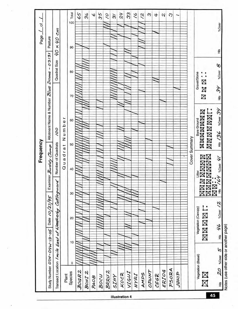

METHODS—Frequency
46 Illustration 5
Nes
ted
Fre
qu
ency
20
Qua
drat
sC
over
Sum
mar
y
Veg
etat
ion
(Bas
al)
% F
req
12
34
% F
req
Hits
Hits
% F
req
Hits
% F
req
Hits
Freq
uenc
y S
umm
ary
by P
lot S
ize
Pag
e
o
f
1918
1716
1513
129
87
65
42
1P
lant
Spe
cies
Tran
sect
Loc
atio
nN
umbe
r of
Qua
drat
sQ
uadr
at S
ize
Stu
dy N
umbe
rD
ate
Exa
min
erA
llotm
ent N
ame
& N
umbe
rP
astu
re
Obs
erva
tions
/Com
men
ts
Not
es (
Use
oth
er s
ide
or a
noth
er p
age)
Hits
%Co
ver
Cry
ptog
amic
cru
st
Hits
%Co
ver
Gra
vel/S
tone
Hits
%Co
ver
Bar
e G
roun
d
Hits
%Co
ver
Litte
r
Veg
etat
ion
(Can
opy)
Hits
%Co
ver
Hits
%Co
ver
Can
opy*
Don
t rec
ord
grou
nd c
over
und
er c
anop
y hi
ts o
f shr
ubs
unde
r 10
ft in
hei
ght
143
1011
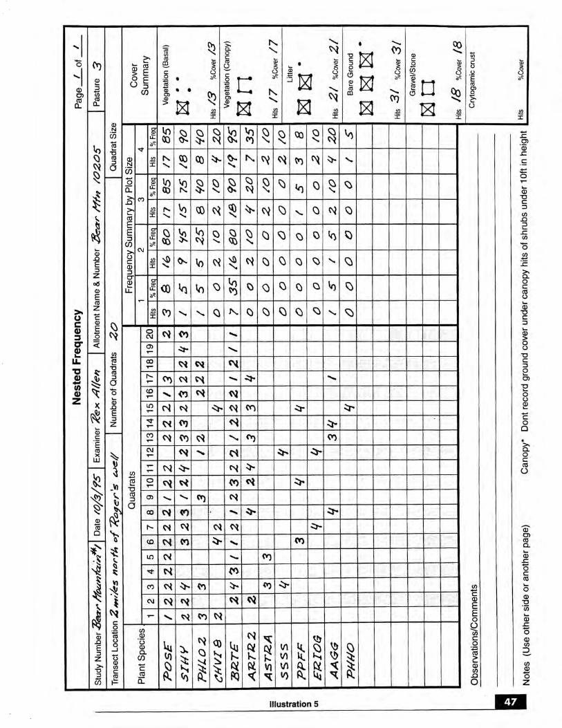
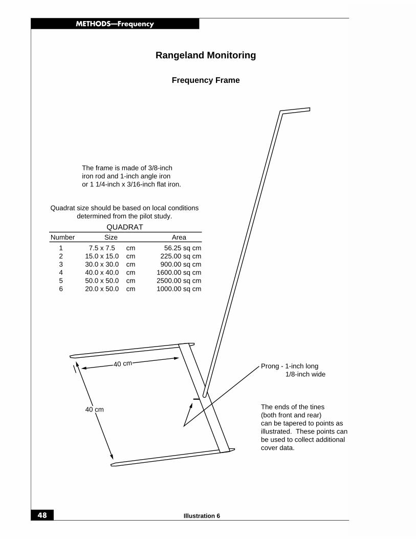
METHODS—Frequency
48 Illustration 6
The frame is made of 3/8-inchiron rod and 1-inch angle ironor 1 1/4-inch x 3/16-inch flat iron.
Prong - 1-inch long1/8-inch wide
The ends of the tines(both front and rear)can be tapered to points asillustrated. These points canbe used to collect additionalcover data.
Frequency Frame
Rangeland Monitoring
40 cm
40 cm
Quadrat size should be based on local conditionsdetermined from the pilot study.
1 7.5 x 7.5 cm 56.25 sq cm2 15.0 x 15.0 cm 225.00 sq cm3 30.0 x 30.0 cm 900.00 sq cm4 40.0 x 40.0 cm 1600.00 sq cm5 50.0 x 50.0 cm 2500.00 sq cm6 20.0 x 50.0 cm 1000.00 sq cm
Number Size
QUADRATArea

49
METHODS—Frequency
Illustration 7
The frames are made of 3/8-inchiron rod and 1-inch angle ironor 1 1/4-inch x 3/16-inch flat iron.Place tines at the proper intervalsalong the rear of the frame andparallel to the sides to create quadratsof smaller sizes.
It is convenient to have a 30-, 20-,15-, 12-, 10-, 6-, and 3-inch quadratavailable. These different size quadratscan be combined in three frames.
The 30-inch and 15-inch quadrats canbe combined in one frame.
The 20-inch and 10-inch quadrats canbe combined in one frame.
The 12-inch, 6-inch, and 3-inch quadratscan be combined in one frame.
The ends of the tines(both front and rear)are tapered to pointsas illustrated. Thesepoints are used to collectcover data.
Rangeland Monitoring
12 in.
6 in.
3 in.
6 in.
3 in.
12 in.
Nested Plot Frame
METHODS—Dry Weight Rank
50
C. Dry Weight Rank Method
1. General Description The Dry Weight Rank method is used to determinespecies composition. It consists of observing various quadrats and ranking thethree species which contribute the most weight in the quadrat.
It is important to establish a photo plot (see Section V.A) and take both close-upand general view photographs. This allows the portrayal of resource values andconditions and furnishes visual evidence of vegetation and soil changes over time.
2. Areas of Use This method has been tested in a wide variety of vegetation typesand is generally considered suitable for grassland/small shrubs types or understorycommunities of large shrub or tree communities. It does not work well on largeshrubs and trees.
3. Advantages and Limitations
a One advantage of the Dry Weight Rank Method is that a large number ofsamples can be obtained very quickly. Another advantage is that it deals withestimates of production, which allows for better interpretation of the data tomake management decisions. It can be done in conjunction with frequency,canopy cover, or comparative yield methods. Because it is easier to rank the topthree species in a quadrat, there is less observer bias.
b The limitation with this technique is that, by itself, it will not give a reliableestimate of plant standing crop, and it assumes there are few empty quadrats.In many large shrub or sparse desert communities, a high percentage of quadratsare empty or have only one species present. The quadrat size required toaddress these concerns is often impractical.
4. Equipment The following equipment is needed (see also the equipment listed inSection V.A, page 31, for the establishment of the photo plot):
• Study Location and Documentation Data form (see Appendix A)• Dry Weight Rank form (see Illustration 8)• Quadrat frame• Hammer• Permanent yellow or orange spray paint• One stake: 3/4 - or 1-inch angle iron not less than 16 inches long• Compass• Steel post and driver
5. Training Examiners must be able to identify the plants. Experience in weightestimate is desirable, but those with experience must break the habit of assigningpercentages and just rank the species, as well as not debating over the close calls.The large number of sampling units tends to reduce the problems with close calls.
6. Establishing Studies
a Site Selection The most important factor in obtaining usable data is select-ing representative areas (critical or key areas) in which to run the study

51
METHODS—Dry Weight Rank
(see Section II.D). Study sites should be located within a single plant communitywithin a single ecological site. Transects and sampling points need to be randomlylocated within the critical or key areas (see Section III).
b Pilot Studies Collect data on several pilot studies to determine the number ofsamples (transects or observation points) and the number and size of quadratsneeded to collect a statistically valid sample (see Section III.B.8).
c Selecting Quadrat Size Adapt the size and shape of quadrats to the vegetationcommunity to be sampled.
(1) Select a plot size on the premise that most plots should contain threespecies.
(2) Determine the proper size quadrat to use by doing preliminary samplingwith different size frames (see Illustration 6).
(3) Use the same size quadrat throughout a study and for rereading the study.If frequencies approach the extremes of either 0 or 100 percent, it may benecessary to change the quadrat size.
d Number of Studies At least one Dry Weight Rank study should be establishedon each study site, depending on the objectives; establish more if needed (seeSections II.D and III.B). Evaluate the rangeland plant communities wherestudies will be located and determine the number of transects and quadratsneeded. The purpose is to collect the best possible sample for the greatestnumber of species in any plant community.
e Study Layout The Dry Weight Rank data can be collected using the baseline,macroplot, or linear study designs described in Section III.A.2 beginning onpage 8. The linear technique is the one most often used.
f Reference Post or Point Permanently mark the location of each study with areference post and a study location stake (see beginning of Section III).
g Study Identification Number studies for proper identification to ensure thatthe data collected can be positively associated with specific sites on the ground(see Appendix B).
h Study Documentation Document pertinent information concerning the studyon the Study Location and Documentation Data form (see beginning of SectionIII and Appendix A).
7. Taking Photographs The directions for establishing photo plots and for takingclose-up and general view photographs are given in Section V.A.
8. Sampling Process In addition to collecting the specific study data, generalobservations should be made of the study sites (see Section II.F).
Determine the transect bearing and select a prominent distant landmark such as apeak, rocky point, etc., that can be used as the transect bearing point.

METHODS—Dry Weight Rank
52
After the quadrat location has been determined, the observer decides which threespecies in the quadrat have the greatest yield of current year’s growth on a drymatter basis. The species with the highest yield is given a rank of 1, the next 2,and the third highest a 3. Data are record by quadrat on the Dry Weight Rankform, Illustration 8. All other species present are ignored. If there are not threespecies present in the quadrat, a multiple rank is assigned.
The Dry Weight Rank method assumes that a rank of 1 corresponds to 70%composition, rank 2 to 20%, and rank 3 to 10%. If only one species is found in aquadrat, it would be ranked 1, 2 and 3 (100%). If two species are found, one maybe given ranks of 1 and 2 (90%), ranks 1 and 3 (80%), or ranks 2 and 3 (30%),depending on the relative weight for the two species (see Illustration 8). For eachspecies, record the number of 1, 2, or 3 ranks received in the sample.
Data can also be collected and recorded for each quadrat for use in conjunctionwith the Comparative Yield Method.
9. Calculations
a For each species multiply the number of ranks of 1, 2, and 3 by 7, 2, and 1,respectively, and record under the appropriate weight column. Add theamounts in the weight columns of each species and record in the weightedcolumn.
b Total the weighted column for all species. The total of this column will alwaysbe ten times the number of quadrats.
c Divide the value recorded for each species in the weighted column by the totalof the weighted column to get percent composition for each species. Percentcomposition, by definition, should total 100 percent.
10. Data Analysis Chi Square analysis can be used to determine if the frequencyof each species in each rank tally group (1,2, or 3) has changed from one samplingperiod to another. Each species must be analyzed separately.
11. References
Despain, D.W., P.R. Ogden, and E.L. Smith. 1991. Plant frequency sampling formonitoring rangelands. In: G.B. Ruyle, ed. Some Methods for MonitoringRangelands and other Natural Area Vegetation. Extension Report 9043,University of Arizona, College of Agriculture, Tucson, AZ.

53
METHODS—Dry Weight Rank
Illustration 8
Spe
cies
Qua
drat
12
34
56
78
910
1112
1314
1516
1718
1920
1
Ran
k Ta
lly
23
Wei
ghte
d%
Com
p.
Stu
dy N
umbe
rD
ate
Exa
min
erA
llotm
ent N
ame
& N
umbe
rP
astu
re
Tran
sect
Loc
atio
nN
umbe
r of
Qua
drat
sQ
uadr
at S
ize
Obs
erva
tions
/Com
men
ts
Dry
Wei
gh
t R
ank
Pag
e
o
f
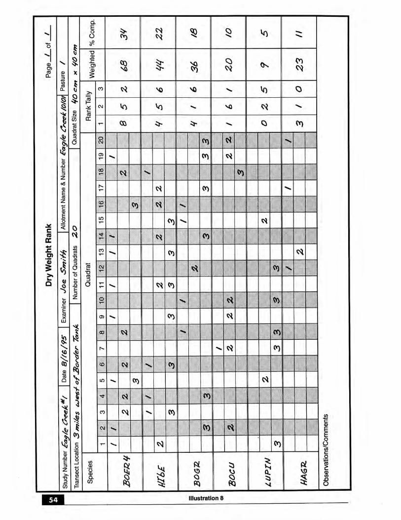

55
METHODS—Daubenmire
D. Daubenmire Method
1. General Description The Daubenmire method consists of systematicallyplacing a 20- x 50-cm quadrat frame along a tape on permanently located transects(see Figure 4 on page 13). The following vegetation attributes are monitored usingthe Daubenmire method:
• Canopy cover• Frequency• Composition by canopy cover
It is important to establish a photo plot (see Section V.A) and take both close-upand general view photographs. This allows the portrayal of resource values andconditions and furnishes visual evidence of vegetation and soil changes over time.
2. Areas of Use This method is applicable to a wide, variety of vegetation types aslong as the plants do not exceed waist height.
3. Advantages and Limitations This method is relatively simple and rapid touse. A limitation is that there can be large changes in canopy cover of herbaceousspecies between years because of climatic conditions, with no relationship to theeffects of management. In general, quadrats are not recommended for estimatingcover (Floyd and Anderson 1987; Kennedy and Addision 1987). This methodcannot be used to calculate rooted frequency.
4. Equipment The following equipment is needed (see also the equipment listedin Section V.A, page 31, for the establishment of the photo plot):
• Study Location and Documentation Data form Appendix A)• Daubenmire forms (see Illustration 9 and 10)• Hammer• Permanent yellow or orange spray paint• Two stakes: 3/4 - or 1-inch angle iron not less than 16 inches long• Tape: 100- or 200-foot, delineated in tenths and hundreds, or a metric tape of
the desired length.• Steel pins (reinforcement bar) for marking zero, mid, and end points of the transect• Frame to delineate the 20- x 50-cm quadrats (see Illustration 11)• Compass• Steel post and driver
5. Training The accuracy of data depends on the training and ability of theexaminers. Examiners must be able to identify the plant species. They mustreceive adequate and consistent training in laying out transects and makingcanopy coverage estimates using the frame.
6. Establishing Studies Careful establishment of studies is a critical element inobtaining meaningful data (see Section III).
a Site Selection The most important factor in obtaining usable data is selectingrepresentative areas (critical or key areas) in which to run the study (see SectionII.D). Study sites should be located within a single plant community within a

METHODS—Daubenmire
56
single ecological site. Transects and sampling points need to be randomlylocated within the critical or key areas (see Section III).
b Pilot Studies Collect data on several pilot studies to determine the number ofsamples (transects or observation points) and the number and size of quadratsneeded to collect a statistically valid sample (see Section III.B.8).
c Number of Studies Establish a minimum of one study on each study site;establish more if needed (see Section II.D and III.B).
d Study Layout Data can be collected using the baseline, macroplot, or linearstudy designs described in Section III.A.2 beginning on page 8. The lineartechnique is the one most often used.
(1) Align a tape (100-, or 200-foot, or metric equivalent) in a straight line bystretching it between the transect location and the transect bearing stakes.Do not allow vegetation to deflect the alignment of the tape. A spring andpulley may be useful to maintain a straight line. The tape should bealigned as close to the ground as possible.
(2) Drive steel pins almost to the ground surface at the zero point on the tapeand at the end of the transect. A pin may also be driven into the ground atthe midpoint of the transect. (see Figure 4 on page 13)
e Reference Post or Point Permanently mark the location of each study with areference post and a study location stake (see beginning of Section III).
f Study Identification Number studies for proper identification to ensure thatthe data collected can be positively associated with specific sites on the ground(See Appendix B).
g Study Documentation Document pertinent information concerning the studyon the Study Location and Documentation Data form (see beginning of Section IIIand Appendix A).
7. Taking Photographs The directions for establishing photo plots and for takingclose-up and general view photographs are given in Section V.A.
8. Sampling Process In addition to collecting the specific studies data, generalobservations should be made of the study sites (see Section II.F).
a Cover Classes This method uses six separate cover classes (Daubenmire 1959).The cover classes are:
Cover Class Range of Coverage Midpoint of Range1 0 - 5% 2.5%2 5 - 25% 15.0%3 25 - 50% 37.5%4 50 - 75% 62.5%5 75 - 95% 85.0%6 95 - 100% 97.5%

57
METHODS—Daubenmire
b Ten Cover Classes Where narrower and more numerous classes are preferred,a ten-cover class system can be used.
c Collecting Cover Data As the quadrat frame is placed along the tape at thespecified intervals, estimate the canopy coverage of each plant species. Recordthe data by quadrat, by species, and by cover class on the Daubenmire form (seeIllustration 9). Canopy coverage estimates can be made for both perennial andannual plant species.
(1) Observe the quadrat frame from directly above and estimate the coverclass for all individuals of a plant species in the quadrat as a unit. All otherkinds of plants are ignored as each plant species is considered separately.
(2) Imagine a line drawn about the leaf tips of the undisturbed canopies (ignor-ing inflorescence) and project these polygonal images onto the ground. Thisprojection is considered “canopy coverage.” Decide which of the classes thecanopy coverage of the species falls into and record on the form.
(3) Canopies extending over the quadrat are estimated even if the plants arenot rooted in the quadrat.
(4) Collect the data at a time of maximum growth of the key species.
(5) For tiny annuals, it is helpful to estimate the number of individuals thatwould be required to fill 5% of the frame (the 71- x 71-mm area). A quickestimate of the numbers of individuals in each frame will then provide anestimate as to whether the aggregate coverage falls in Class 1 or 2, etc.
(6) Overlapping canopy cover is included in the cover estimates by species;therefore, total cover may exceed 100 percent. Total cover may not reflectactual ground cover.
9. Calculations Make the calculations and record the results in the appropriatecolumns on the Daubenmire form (see Illustrations 9 and 10).
a Canopy Cover Calculate the percent canopy cover by species as follows:
(1) On the Daubenmire form (Illustration 9) count the number of quadrats ineach of the six cover class (by species) and record in the Number columnon the Daubenmire Summary form (Illustration 10).
(2) Multiply this value times the midpoint of the appropriate cover class(Illustration 10).
(3) Total the products for all cover classes by species.
(4) Divide the sum by the total number of quadrats sampled on the transect.
(5) Record the percent cover by species on the form.
METHODS—Daubenmire
58
b Frequency Calculate the percent frequency for each plant species by dividingthe number of occurrences of a plant species (the number of quadrats in whicha plant species was observed) by the total number of quadrats sampled alongthe transect. Multiply the resulting value by 100. Record the percent fre-quency on the form (Illustration 10).
c Species Composition With this method, species composition is based oncanopy cover of the various species. It is determined by dividing the percentcanopy cover of each plant species by the total canopy cover of all plant species.Record the percent composition on the form (Illustration 10).
10. Data Analysis Tests should be directed at detecting changes in cover of thespecies and/or in major ground cover classes. Tests for changes in minor specieswill have low power to detect change. If quadrats are spaced far enough apart oneach transect so as to be considered independent, the quadrat can be analyzed asthe sampling unit. Otherwise, the transects should be considered the samplingunits. If the transects are treated as the sampling unit, and given that the transectsare permanent, either the paired t-test or the nonparametric Wilcoxon signed ranktest should be used to test for change between two years. Repeated measuresANOVA can be used to test for differences between 3 or more years. If thequadrats are treated as the sampling units, care must be taken to ensure they arepositioned the same along each transect in each year of measurement. A pairedt-test, Wilcoxon signed rank test, or ANOVA is then used as described above fortransects.
11. References
Daubenmire, Rexford. 1959. A Canopy-coverage method of vegetational analysis.Northwest Science 33:43-64.
——— 1968. Plant communities: a textbook of plant synecology. Harper andRow, New York. 300 p.
USDI, Bureau of Land Management. 1985. Rangeland monitoring - Trend StudiesTR4400-4.

59
METHODS—Daubenmire
Illustration 9
Qua
drat
Pag
e
o
fD
aub
enm
ire
15P
lant
Spe
cies
Tran
sect
Num
ber
and
Loca
tion
Num
ber
of Q
uadr
ats
Stu
dy N
umbe
rD
ate
Exa
min
erA
llotm
ent N
ame
& N
umbe
rP
astu
re
2627
2829
3031
3233
3436
3738
3539
4142
4340
4446
4748
4550
49
1416
1317
1819
2021
2223
2425
1211
109
87
65
43
21
Qua
drat
Pla
ntS
peci
es


61
METHODS—Daubenmire
Illustration 10
1-5%
5-25
%
26-5
0%
51-7
5%
76-9
5%
96-1
00%
Dau
ben
mir
e S
um
mar
y
1 2 3 4 5 6
Cov
erC
lass
Stu
dy L
ocat
ion
Num
ber
of Q
uadr
ats
Tota
l can
opy
Num
ber
of S
ampl
es
% c
anop
y co
ver
Spe
cies
com
posi
tion
Freq
uenc
y
Mid
-P
oint
N u m b e r
2.5
15 37.5
62.5
85 97.5
Stu
dy N
umbe
rD
ate
Exa
min
erA
llotm
ent N
ame
& N
umbe
rP
astu
re
P r o d u c t
N u m b e r
P r o d u c t
N u m b e r
P r o d u c t
N u m b e r
P r o d u c t
N u m b e r
P r o d u c t
N u m b e r
P r o d u c t
N u m b e r
P r o d u c t
N u m b e r
P r o d u c t
N u m b e r
P r o d u c t
N u m b e r
P r o d u c t
N u m b e r
P r o d u c t
Spe
cies
Spe
cies
Spe
cies
Pag
e
o
f
Spe
cies
Spe
cies
Spe
cies
Spe
cies
Spe
cies
Spe
cies
Spe
cies
Spe
cies
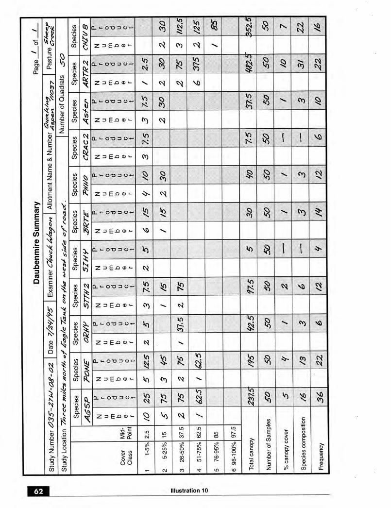
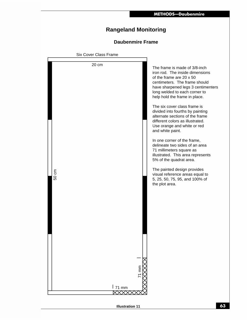
63
METHODS—Daubenmire
Illustration 11
The frame is made of 3/8-inchiron rod. The inside dimensionsof the frame are 20 x 50centimeters. The frame shouldhave sharpened legs 3 centimenterslong welded to each corner tohelp hold the frame in place.
The six cover class frame isdivided into fourths by paintingalternate sections of the framedifferent colors as illustrated.Use orange and white or redand white paint.
In one corner of the frame,delineate two sides of an area71 millimeters square asillustrated. This area represents5% of the quadrat area.
The painted design providesvisual reference areas equal to5, 25, 50, 75, 95, and 100% ofthe plot area.
Six Cover Class Frame
20 cm
50 c
m
71 m
m
71 mm
Daubenmire Frame
Rangeland Monitoring
METHODS—Line Intercept
64
E. Line Intercept Method
1. General Description The Line Intercept method consists of horizontal, linearmeasurements of plant intercepts along the course of a line (tape). It is designedfor measuring grass or grass-like plants, forbs, shrubs, and trees. The followingvegetation attributes are monitored with this method:
• Foliar and basal cover• Composition (by cover)
It is important to establish a photo plot (see Section V.A) and take both close-upand general view photographs. This allows the portrayal of resource values andconditions and furnishes visual evidence of vegetation and soil changes over time.
2. Areas of Use This method is ideally suited for semiarid bunchgrass-shrubvegetation types.
3. Advantages and Limitations The Line Intercept method is best suitedwhere the boundaries of plant growth are relatively easy to determine. It can beadapted to sampling varying densities and types of vegetation. It is not welladapted, however, for estimating cover on single-stemmed species, dense grasslandsituations, litter, or gravel less than 1/2 inch in diameter. It is best suited to esti-mating cover on shrubs.
4. Equipment The following equipment is needed (see also the equipment listed inSection V.A, page 31, for the establishment of the photo plot):
• Study Location and Documentation Data form (see Appendix A)• Line Intercept form (see Illustration 12)• Hammer• Permanent yellow or orange spray paint• Two stakes: 3/4 - or 1-inch angle iron not less than 16 inches long.• Two tapes: 100- or 200-foot, delineated in tenths and hundredths, or a metric
tape of the desired length• Compass• Steel post and driver
5. Training A minimum of training is needed to make sure the examiners under-stand how to lay out baselines and transects and how to make the measurements.The examiner must also be able to identify the plant species.
6. Establishing Studies Careful establishment of studies is a critical element inobtaining meaningful data (see Section III).
a Site Selection The most important factor in obtaining usable data is selectingrepresentative areas (critical or key areas) in which to run the study (seeSection II.D). Study sites should be located within a single plant communitywithin a single ecological site. Transects and sampling points need to be randomlylocated within the critical or key areas (see Section III).
65
METHODS—Line Intercept
b Pilot Studies Collect data on several pilot studies to determine the number ofsamples (transects or observation points) and the number and size of quadratsneeded to collect a statistically valid sample (see Section III.B.8).
c Number of Transects Establish the minimum number of transects to achievethe desired level of precision for the key species in each study site (see Section III.B).
d Length of Transect The length of a transect is based on the density andhomogeneity of the vegetation. If the vegetation is sparse, a longer transect isneeded. Transects may be any length (eg. 100 feet, 200 feet, or even longer).
e Study Layout Line Intercept data can be collected using either the baseline orlinear study design described in Section III.A.2 beginning on page 8. Thebaseline technique is the recommended study design.
(1) The study location stake is placed at the beginning of the baseline. Afterdetermining the bearing of the study, a stake is placed at the end of thebaseline. Transects are run perpendicular to and at random distances alongthe baseline. Transect location stakes are placed at the beginning and endof each transect. The distance between the stakes dependents on the lengthof the transect. The height of the stakes depends on the height of thevegetation. (Directions for randomly selecting the location of transects to berun off of a baseline using random number tables are given in Appendix D).
Transect location stakes may be left in place as permanent markers orremoved at the conclusion of the study. Permanently marking transectswill result in greater power to detect change.
(2) Stretch the transect tapes between stakes as close to the ground as possible,with the zero point of the tape aligned on the baseline (the beginning pointof the transect). Do not allow vegetation to deflect the alignment of the tape.
f Reference Post or Point Permanently mark the location of each study with areference post and a study location stake (see beginning of Section III).
g Study Identification Number studies for proper identification to ensure thatthe data collected can be positively associated with specific sites on the ground.(see Appendix B).
h Study Documentation Document pertinent information concerning the studyon the Study Location and Documentation Data form (see beginning of SectionIII and Appendix A).
7. Taking Photographs The directions for establishing photo plots and for takingclose-up and general view photographs are given in Section V.A.
8. Sampling Process In addition to collecting the specific studies data, generalobservations should be made of the study sites (see Section II.F).
Proceed down the tape stretched along the transect line and measure the horizontallinear length of each plant that intercepts the line. Measure grasses and grass-like
METHODS—Line Intercept
66
plants, along with rosette-forming plants, at ground level. For forbs, shrubs, andtrees, measure the vertical projection of the foliar cover intercepting one side ofthe tape. Be sure not to inadvertently move the tape to include or exclude certainplants. If the measurements are made in 10ths and 100ths of feet, the totals areeasily converted to percentages. The measurements are recorded by species on theLine Intercept form (Illustration 12).
9. Calculations Make the calculations and record the results on the Line Interceptform (see Illustration 12).
a Cover
(1) Calculate the percent cover of each plant species by totaling the interceptmeasurements for all individuals of that species along the transect line andconvert this total to a percent.
(2) Where the measurements are made in 10ths and 100ths of feet along a100-foot transect, the totals for each species are the cover percentages.
(3) Calculate the total cover measured on the transect by adding the coverpercentages for all the species. This total could exceed 100% if the inter-cepts of overlapping canopies are recorded.
b Composition With this method, species composition is based on the percentcover of each species. Calculate percent composition by dividing the percentcover for each plant species by the total cover for all plant species.
10. Data Analysis It is important to realize that each transect is a single samplingunit. For trend analysis permanent sampling units are suggested. If permanenttransects are monitored, use the appropriate paired analysis technique. Use eithera paired t-test or the nonparametric Wilcoxon signed rank test when testing forchange between years. When comparing more than two sampling periods, userepeated measures ANOVA. If the transects are not permanently marked, use theappropriate nonpaired test.
11. References
Brun, Jorge M. and Thadis W. Box. 1963. Comparison of line intercepts andrandom point frames for sampling desert shrub vegetation. J. Range Manage.16:21-25.
Buckner, D.L. 1985. Point-Intercept Sampling in Revegetation Studies: MaximizingObjectivity and Repeatability. Paper presented at American Society for SurfaceMining and Reclamation Meeting, Denver, CO. 1985.
Canfield, R.H. 1941. Application of the line interception method in samplingrange vegetation. J. Forestry 39:388-394.
Canfield, R.H. 1944. Measurement of grazing use by the line intercept Method.Jour. For. 42(3):192-194

67
METHODS—Line Intercept
Hanley, Thomas A. 1978. A comparison of the line-interception and quadratestimation methods of determining shrub canopy coverage. J. Range Manage.31:60-62.
Kinsinger, Floyd E., Richard E. Eckert, and Pat 0. Currie. 1960. A comparison ofthe line-interception, variable-plot, and loop methods as used to measureshrub-crown cover. J. Range Manage. 13:17-21.
USDI, Bureau of Land Management. 1985. Rangeland monitoring - Trend studiesTR4400-4.

METHODS—Line Intercept
68 Illustration 12
Lin
e In
terc
ept
Pag
e
o
f
Line
Len
gth
Tran
sect
Loc
atio
n
Tota
ls
% C
over
% C
omp
Stu
dy N
umbe
rD
ate
Exa
min
erA
llotm
ent N
ame
& N
umbe
rP
astu
re
NO
TE
S(U
se o
ther
sid
e or
anot
her
page
, if n
eces
sary
)
Gra
ss S
peci
esFo
rb S
peci
esS
hrub
Spe
cies
NO
TE
S
Tota
ls
100%


METHODS—Step Point
70
F. Step-Point Method
1. General Description The Step-Point Method involves making observationsalong a transect at specified intervals, using a pin to record cover “hits.” It mea-sures cover for individual species, total cover, and species composition by cover.
It is important to establish a photo plot (see Section V.A) and take both close-upand general view photographs. This allows the portrayal of resource values andconditions and furnishes visual evidence of vegetation and soil changes over time.
2. Areas of Use This method is best suited for use with grasses and forbs, as wellas low shrubs. The greater the structure to the community, the more difficult itbecomes to determine “hits” due to parallax, observer bias, wind, etc. This methodis good for an initial overview of an area not yet subjected to intensive monitoring.
3. Advantages and Limitations This method is relatively simple and easy touse as long as careful consideration is given to the vegetation type to which it isapplied. It is suitable for measuring major characteristics of the ground and veg-etation cover of an area. Large areas can easily be sampled, particularly if thecover is reasonably uniform. It is possible to collect a fairly large number ofsamples within a relatively short time.
A limitation of this method is that there can be extreme variation in the datacollected among examiners when sample sizes are small. Tall or armored vegeta-tion reduces the ability to pace in a straight line, and the offset for obstructionsdescribed in the procedures adds bias to the data collection by avoiding certaincomponents of the community. Another limitation is that less predominant plantspecies may not be hit on the transects and therefore do not show up in the studyrecords. The literature contains numerous studies utilizing point interceptprocedures that required point densities ranging from 300 to 39,000 in order toadequately sample for minor species. One major consideration in the use of thismethod is to assure that a sharpened pin is used and that only the point is used torecord “hits.” Pins have finite diameters and therefore overestimate cover (Goodall1952). Another limitation of this method is that statistical analysis of the data issuspect unless two and preferably more transects are run per site (see Section III -Study Design and Analysis).
4. Equipment The following equipment is needed (see also the equipment listed inSection V.A, page 31, for the establishment of the photo plot):
• Study Location and Documentation Data form (see Appendix A)• Cover Data form (see Illustration 13)• Permanent yellow or orange spray paint• Tally counter (optional)• One stake: 3/4- or 1-inch angle iron not less than 16 inches long• 3-foot long, 3/16th-inch diameter sharpened pin• Compass• Steel post and driver
5. Training A minimum amount of training is needed for this method. Examinersmust be able to identify the plant species, be familiar with the ground-level cover
71
METHODS—Step Point
categories, know how to collect canopy or foliar cover data, and know how tocollect cover data using a pin and notch in the boot.
6. Establishing Studies Careful establishment of studies is a critical element inobtaining meaningful data.
a Site Selection The most important factor in obtaining usable data is selectingrepresentative areas (critical or key areas) in which to run the study (see SectionII.D). Study sites should be located within a single plant community within asingle ecological site. Transects and sampling points need to be randomlylocated within the critical or key areas. (see Section III).
b Pilot Studies Collect data on several pilot studies to determine the number ofsamples (transects or observation points) and the number and size of quadratsneeded to collect a statistically valid sample (see Section III.B.8).
c Number of Transects Establish the minimum number of transects to achievethe desired level of precision (see Section III.B).
d Study Layout Data can be collected using either the baseline or linear studydesigns described in Section III.A.2 beginning on page 8. The linear techniqueis the one most often used.
e Reference Post or Point Permanently mark the location of each study with areference post and a study location stake (see beginning of Section III).
f Study Identification Number studies for proper identification to ensure thatthe data collected can be positively associated with specific sites on the ground(see Appendix B).
g Study Documentation Document pertinent information concerning the studyon the Study Location and Documentation Data form (see beginning of Section IIIand Appendix A).
7. Taking Photographs The directions for establishing photo plots and for takingclose-up and general view photographs are given in Section V.A.
8. Sampling Process In addition to collecting the specific studies data, generalobservations should be made of the study sites (see Section II.F).
a Running a Transect Determine the transect bearing and select a prominentdistant landmark such as a peak, rocky point, etc., that can be used as thetransect bearing point.
(1) Start a transect by randomly selecting a point along the transect bearingand reading the first hit (observation point).
(2) Read hits at specified intervals by placing the heel of the boot on theground with the sole of the boot at a 30-degree angle to the ground. Placethe pin into the 3/16th inch wide by 1/8th inch deep notch in the toe of
METHODS—Step Point
72
the boot and vertically lower the pin until it either intersects an herbaceousplant or the ground for the specified number of hits. It is recommendedthat the interval be a minimum of 5 paces. To lengthen the transect,increase the distance between hits (10 paces, 20 paces, etc.).
(3) When obstructions such as juniper trees, cholla cactus, or ledge rock, etc.,are encountered, sidestep at 90˚ from the transect line and continue pacingparallel to the transect to avoid the obstructions. Return to the originaltransect line as soon as possible by sidestepping at 90˚ in the oppositedirection. Continue pacing along the transect bearing. If the obstruction(juniper tree, cholla cactus, or ledge rock) is determined to be a highlyimportant component of the community, this information can be recordedqualitatively on the back of the form.
(4) In most cases, do not count hits along portions of a transect that have beenunnaturally disturbed, such as roads or trails. When such areas areencountered, proceed three paces past the disturbance before resuming thereading of hits along the transect line.
b Collecting Cover Data At each observation point, identify the ground levelor basal hit with the point of the pin and record the data by dot count tally bycategory and/or plant species code in the appropriate section of the Cover Dataform (see Illustrations 13 and 14). If there is a vegetation canopy layer, lowerthe pin through the vegetation until a basal or ground level hit is determined.Record the basal or ground level hit and any subsequent vegetation layers thatintersect the pin. For vegetation structure above 3-feet (length of pin), a visualobservation of plant intercepts above the notch in the boot can be made andrecorded as additional canopy or foliar level hits on the data form.
(1) Ground-level or basal hits
(a) Ground-level hits (excluding basal vegetation hits) will fall into fourcover categories. They can be redefined and/or additional categoriesadded, depending on the data needed. The four categories are:
L - Litter
B - Bare ground
G - Gravel (particle sizes between 1/12 inch and 10 inches)
S - Stone (greater than 10 inches)
(b) Record the ground-level hits by dot count tally by ground-level covercategory in the Ground-Level Cover section of the form, except wherethere are ground-level and, basal or canopy cover hit combinations. Inthis situation, use the Basal and Canopy/Foliar Cover section of the form.
(c) Basal hits on live vegetation are identified by species (includes mossesand lichens more than 1/16 inch thick). To count as a basal hit on livevegetation, the plant crown at or below a l-inch height above theground MUST be intercepted by the pin.
73
METHODS—Step Point
(d) Enter the appropriate plant species code in the Basal or Ground-LevelColumn in the Basal and Canopy/Foliar Cover section of the form.
(e) Enter a dot count tally for each basal hit on a species in the Dot CountColumn in the Basal and Canopy/Foliar Cover section of the formwhen the plant species code is first entered on the form. Enter anadditional dot count tally each time there is a basal hit on that specieson the transect, except where there are basal and canopy/foliar coverhit combinations.
(2) Ground-level or basal and canopy/foliar cover hit combinations
(a) Identify the ground-level or basal hit, as well as any canopy coverhit(s) below 3 feet in height, intercepted at each point by the pin. Forcanopy cover above 3 feet, use line-of-sight observations directlyperpendicular to the notch in the boot.
(b) Enter the appropriate ground-level cover category code and/or plantspecies code for each level of hit (up to four levels) in the appropriatecolumns in the Basal and Canopy/Foliar Cover section of the form (seeIllustration 13).
(c) Enter a dot count tally for each ground-level or basal and canopy/foliarcover hit combination when it is first entered on the form and eachtime this same combination is encountered on the transect.
(d) Enclose plant species codes for vegetation cover hits more than 20 feetabove ground level in brackets [ ].
9. Calculations Calculate the percent cover for each cover category by dividingthe number of hits for each category by the total number of hits for all categories,including hits on vegetation.
a Ground Cover Ground cover is determined by dividing the total number ofhits for all categories except bare ground by the total number of hits (includingbare ground).
b Canopy/Foliar Cover Canopy/Foliar cover is determined by dividing the totalnumber of hits on vegetation (includes all basal and canopy/foliar hits) by thetotal number of hits.
c Basal Cover Basal cover is determined by dividing the number of basal hits bythe total number of hits.
10. Data Analysis
a When transects are the sampling units: For trend analysis, permanent samplingunits are suggested. If permanent transects are monitored, use the appropriatepaired analysis technique to compare change in average cover by species andcover class. When comparing more than two sampling periods, use repeated
METHODS—Step Point
74
measures ANOVA. If the transects are not permanently marked, use theappropriate nonpaired test.
b When points are the sampling units: To determine if the change betweensampling periods is significant, use Chi Square analysis of variance for cover data.
11. References
Bonham, C.D. 1989. Measurements for Terrestrial Vegetation, John Wiley andSons, New York, NY. 338 p.
Evans, Raymond A. and R. Merton Love. 1957. The step-point method of sam-pling—a practical tool in range research. J. Range Manage. 10:208-212.
Goodall, D.W. 1952. Some considerations in the use of point quadrats for theanalysis of vegetation. Aust. J. Sci. Res., Series B 5:1-41
Mueller-Dombois, Dieter and Heinz Ellenberg. 1974. Aims and methods ofvegetation ecology. John Wiley & Sons, New York, NY. 547 p.
USDI, Bureau of Land Management. 1985. Rangeland monitoring - Trend studiesTR4400-4.

75
METHODS—Step Point
Illustration 13
B L G SGround-Level Cover
DotCount
TotalHits
% Cover
Category
Basal and Canopy/Foliar Cover
Bsl or Grnd-Lev Level 1 Level 2 Level 3 Dot Count Total Hits
Litter Vegetation TotalBare Gravel StoneGround (2mm-10") (>10")
Notes (use other side or another page)
Total
Cover Data
Study Number Date Examiner Pasture
Allotment Name & Number Study Location Number of Points
Page of

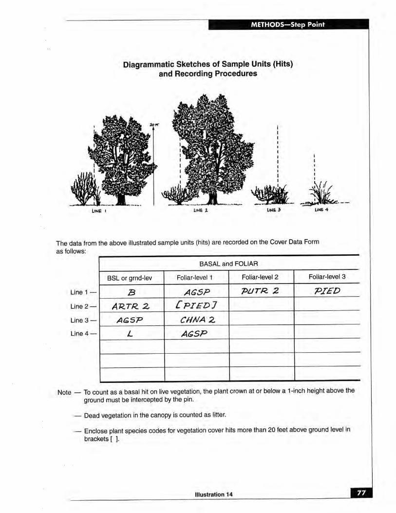

METHODS—Point Intercept
78
G. Point-Intercept Method - Sighting Devices, Pin Frames,and Point Frames
1. General Description The Point-Intercept method consists of employing a sightingdevice or pin/point frame along a set of transects to arrive at an estimate of cover. Itmeasures cover for individual species, total cover, and species composition by cover.
It is important to establish a photo plot (see Section V.A) and take both close-upand general view photographs. This allows the portrayal of resource values andconditions and furnishes visual evidence of vegetation and soil changes over time.
2. Areas of Use This method is suited to all vegetation types less than about 1.5meters in height. This is because sighting devices and pin/point frames require theobserver to look down on the vegetation from above in a vertical line with theground. If the sighting device allows upward viewing, the method can also be usedto estimate the canopy cover of large shrubs and trees.
3. Advantages and Limitations Point interception measurements are highlyrepeatable and lead to more precise measurements than cover estimates usingquadrats. The method is more efficient than line intercept techniques, at least forherbaceous vegetation, and it is the best method of determining ground cover andthe cover of the more dominant species. Given the choice between sightingdevices and pin/point frames, the optical sighting device is preferable.
A limitation of point-intercept sampling is the difficulty in picking up the minor species inthe community without using a very large number of points. In addition, wind will increasethe time required to complete a study because of the need to view a stationary plant.
One limitation that is specific to the use of point frames is that a given number ofpoints grouped in frames gives less precise estimates of cover than the same number ofpoints distributed individually (Goodall 1952; Greig-Smith 1983). In fact, single-pinmeasurements require only one-third as many points as when point frames are used(Bonham 1989). Another problem with frames is that they overestimate the cover oflarge or clumped plants because the same plant is intercepted by different points onthe same frame (Bonham 1989). This problem is overcome with the methoddescribed here by treating the frames as the sampling units (rather than using theindividual points as sampling units). However, this approach doesn’t change thefact that more points must be read than when the points are independent.
Use of a pin frame device (as opposed to a grid frame made of crossing strings) willresult in overestimation of cover because the pins have finite diameter. The use ofa sharpened pin will greatly reduce overestimation when only the point of the pinis used to record a hit or a miss.
4. Equipment The following equipment is needed (see also the equipment listed inSection V.A, page 31, for the establishment of the photo plot):
• Study Location and Documentation Data form (see Appendix A)• Cover Data form (see Illustration 13 on page 75)• Sighting device (see Illustration 15)4
4 A sighting device is available commercially from ESCO, P.O. Box 18775, Boulder, Colorado 80308.

79
METHODS—Point Intercept
• Tripod for mounting sighting device• Panhead for tripod (makes possible rapid positioning of sighting device)• Pin or point frame. This can be a pin frame (see Illustration 16), usually with
10 pins (Bonham 1989; Pieper 1973) or a point frame (see Illustration 17),consisting of two superimposed string grids mounted one above the other onthree adjustable legs (Floyd and Anderson 1983). The design of Floyd andAnderson (1983) produces a sighting grid of 36 points per frame.
• Hammer• Permanent yellow or orange spray paint• Tally counter (optional)• Two stakes: 3/4 - or 1-inch angle iron not less than 16 inches long• Compass• Steel post and driver• Tape: 50-, 100-, or 200-foot delineated in tenths and hundreds or a metric tape
of the desired length.
5. Training A minimum of training is needed to make sure the examiners under-stand how to lay out baselines and transects and position and read the specificsighting device or pin/point frame being employed. The examiners must also beable to identify the plant species.
6. Establishing Studies Careful establishment of studies is a critical element inobtaining meaningful data.
a Site Selection The most important factor in obtaining usable data is selectingrepresentative areas (critical or key areas) in which to run the study (see SectionII.D). Study sites should be located within a single plant community within asingle ecological site. Transects and sampling points need to be randomlylocated within the critical or key areas (see Section III).
b Pilot Studies Collect data on several pilot studies to determine the number ofsamples (transects or observation points) and the number and size of quadratsneeded to collect a statistically valid sample (see Section III.B.8).
c Study Layout Data can be collected using either the baseline or linear studydesigns described in Section III.A.2 beginning on page 8. The baselinetechnique is the recommended procedure.
d Reference Post or Point Permanently mark the location of each study with areference post and a study location stake (see beginning of Section III).
e Study Identification Number studies for proper identification to ensure thatthe data collected can be positively associated with specific sites on the ground(see Appendix B).
f Study Documentation Document pertinent information concerning the studyon the Study Location and Documentation Data form (see beginning of Section IIIand Appendix A).
7. Taking Photographs The directions for establishing photo plots and for takingclose-up and general view photographs are given in Section V.A.
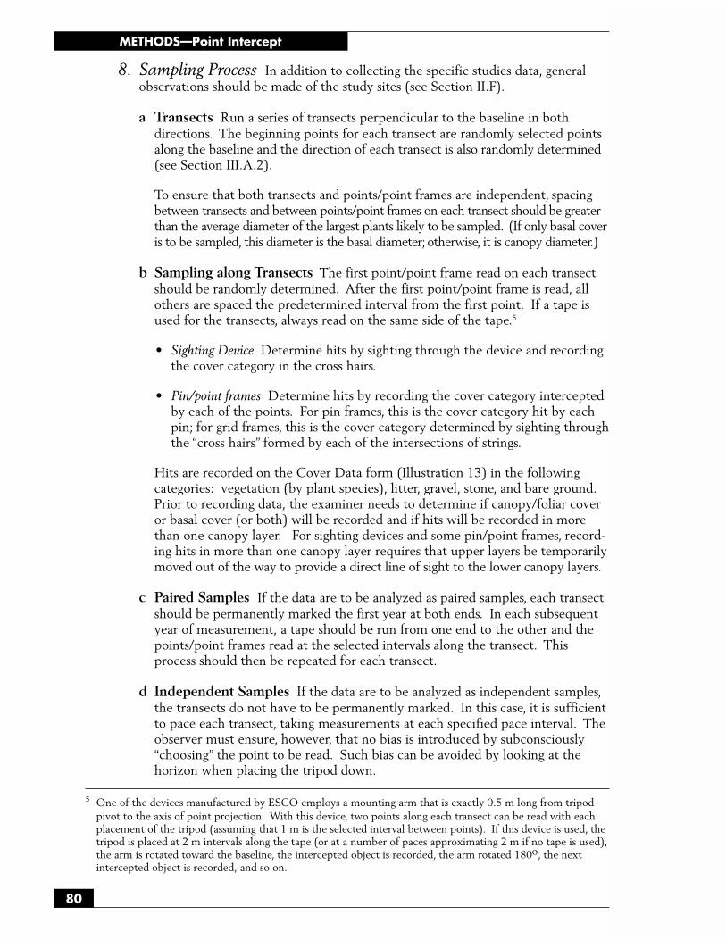
METHODS—Point Intercept
80
8. Sampling Process In addition to collecting the specific studies data, generalobservations should be made of the study sites (see Section II.F).
a Transects Run a series of transects perpendicular to the baseline in bothdirections. The beginning points for each transect are randomly selected pointsalong the baseline and the direction of each transect is also randomly determined(see Section III.A.2).
To ensure that both transects and points/point frames are independent, spacingbetween transects and between points/point frames on each transect should be greaterthan the average diameter of the largest plants likely to be sampled. (If only basal coveris to be sampled, this diameter is the basal diameter; otherwise, it is canopy diameter.)
b Sampling along Transects The first point/point frame read on each transectshould be randomly determined. After the first point/point frame is read, allothers are spaced the predetermined interval from the first point. If a tape isused for the transects, always read on the same side of the tape.5
• Sighting Device Determine hits by sighting through the device and recordingthe cover category in the cross hairs.
• Pin/point frames Determine hits by recording the cover category interceptedby each of the points. For pin frames, this is the cover category hit by eachpin; for grid frames, this is the cover category determined by sighting throughthe “cross hairs” formed by each of the intersections of strings.
Hits are recorded on the Cover Data form (Illustration 13) in the followingcategories: vegetation (by plant species), litter, gravel, stone, and bare ground.Prior to recording data, the examiner needs to determine if canopy/foliar coveror basal cover (or both) will be recorded and if hits will be recorded in morethan one canopy layer. For sighting devices and some pin/point frames, record-ing hits in more than one canopy layer requires that upper layers be temporarilymoved out of the way to provide a direct line of sight to the lower canopy layers.
c Paired Samples If the data are to be analyzed as paired samples, each transectshould be permanently marked the first year at both ends. In each subsequentyear of measurement, a tape should be run from one end to the other and thepoints/point frames read at the selected intervals along the transect. Thisprocess should then be repeated for each transect.
d Independent Samples If the data are to be analyzed as independent samples,the transects do not have to be permanently marked. In this case, it is sufficientto pace each transect, taking measurements at each specified pace interval. Theobserver must ensure, however, that no bias is introduced by subconsciously“choosing” the point to be read. Such bias can be avoided by looking at thehorizon when placing the tripod down.
5 One of the devices manufactured by ESCO employs a mounting arm that is exactly 0.5 m long from tripodpivot to the axis of point projection. With this device, two points along each transect can be read with eachplacement of the tripod (assuming that 1 m is the selected interval between points). If this device is used, thetripod is placed at 2 m intervals along the tape (or at a number of paces approximating 2 m if no tape is used),the arm is rotated toward the baseline, the intercepted object is recorded, the arm rotated 180o, the nextintercepted object is recorded, and so on.

81
METHODS—Point Intercept
9. Calculations Make the calculations and record the results on the Cover Dataform (see Illustration 13, page 75).
a Cover of Individual Plants, Litter, Gravel, Stone, and Bare Ground
(1) Paired samples Calculate the percent cover of each species along eachtransect by totaling all of the “hits” for that species along the transect,dividing the hits by the total number of points along the transect, andmultiplying by 100. Calculate the total percent cover for the species in thesampled area by adding together all the transect cover values for thespecies and dividing by the number of transects. Do the same for litter,gravel, stone, and bare ground.
When point frames are used, the point frames themselves can be analyzedas sampling units. In this case, percent cover of each species is calculatedfor each point frame. Percent cover is calculated by totaling all of the “hits”for that species in one frame, dividing the hits by the total number ofpoints in that frame, and multiplying by 100. In this situation, cover datafor each frame must be recorded separately on one form or on separate forms.
(2) Independent samples: Sighting device and pin frames Calculate thepercent cover of each species in the study area as a whole by totaling allthe “hits” for that species along all of the transects, dividing by the totalnumber of points in the study, and multiplying by 100. Do the same forlitter, gravel, stone, and bare ground.
(3) Independent samples: Point frames For independent samples, the framesthemselves can be considered the sampling units. Calculate the percentcover of each species in each point frame by totaling all the “hits” for thatspecies in the frame, dividing the hits by the total number of points in theframe, and multiplying by 100. Calculate the total percent cover for thespecies in the sampled area by adding together all of the point frame covervalues for the species and dividing by the number of point frames. Do thesame for litter, gravel, stone, and bare ground.
(4) Total vegetation cover Calculate total vegetation cover by adding thestudy area cover percentages for all plant species. This total could exceed100 percent if multiple hits (overlapping canopies) were recorded at eachpoint along the transect.
b Species Composition Species composition is based on the percent cover ofthe various species. Calculate percent composition by dividing the percentcover for each plant species by the total cover for all plant species.
10. Data Analysis The method of data analysis depends upon whether or not thetransects are permanent.
a Permanent Transects If the transects are permanent, the transects or pointframes are the sampling units. Either a paired t test or the nonparametric Wilcoxonsigned rank test is used to test for significant change in average cover between twosampling periods. Repeated measures analysis of variance is used to test forsignificant change in average cover between three or more sampling periods.

METHODS—Point Intercept
82
b Transects Not Permanent If the transects are not permanent, that is, if theyare randomly located in each sampling period, then the samples are indepen-dent and the points can be treated as the sampling units.
Sighting Devices: Analysis consists of a Chi Square contingency table analysisto test for significant change between years in numbers of “hits” on the keyspecies, other plant species, or cover classes.
Point Frames: Analysis consists of testing for significant changes in averagecover between sampling periods using the independent sample t test or thenonparametric Mann Whitney U test. Independent sample analysis of varianceor the nonparametric Kruskal-Wallis test is used to test for significant changes inaverage cover between three or more years.
11. References
Bonham, C.D. 1989. Measurements for Terrestrial Vegetation, John Wiley andSons, 338 p.
Brown, Dorothy. 1954. Methods of surveying and measuring vegetation. Common-wealth Bureau of Pastures and Field Crops. Bulletin No. 42. Commonw. Agr.Bur., Farmham Royal, Bucks, England. 223 p.
Brun, Jorge M. and Thadis W. Box. 1963. Comparison of line intercepts andrandom point frames for sampling desert shrub vegetation. J. RangeManagement. 16:21-25.
Buckner, D.L. 1985. Point-intercept sampling in revegetation studies; maximizingobjectivity and repeatability. Proceedings of the American Society of SurfaceMining and Reclamation. 1985 Annual Meeting, Denver, CO.
Goodall, D.W. 1952. Some considerations in the use of point quadrats for theanalysis of vegetation. Aust. J. Sci. Res., Series B 5:1-41
Greig-Smith, P. 1983. Quantitative plant ecology. 3rd Ed. University of CaliforniaPress Berkeley and Los Angeles.
Floyd, D.A., and J.E. Anderson. 1983. A new point interception frame for estimatingcover of vegetation. Idaho National Engineering Laboratory Radioecology andEcology Programs 1983 Progress Report, pp.107-113
Levy, E.B. and E.A. Madden. 1933. The Point method for Pasture Analysis. NewZealand J. Agric. 46: 267-279.
Mueller-Dombois, Dieter and Heinz Ellenberg. 1974. Aims and methods ofvegetation ecology. John Wiley & Sons, New York. 547 p.
Stanton, F.W. 1960. Ocular Point Frame. J. Range Manage. 13:153.
Winkworth, R.E. and D.W. Goodall. 1962. A Crosswire Sighting Tube for Point-Quadrat Analysis. Ecology 43:342-343.
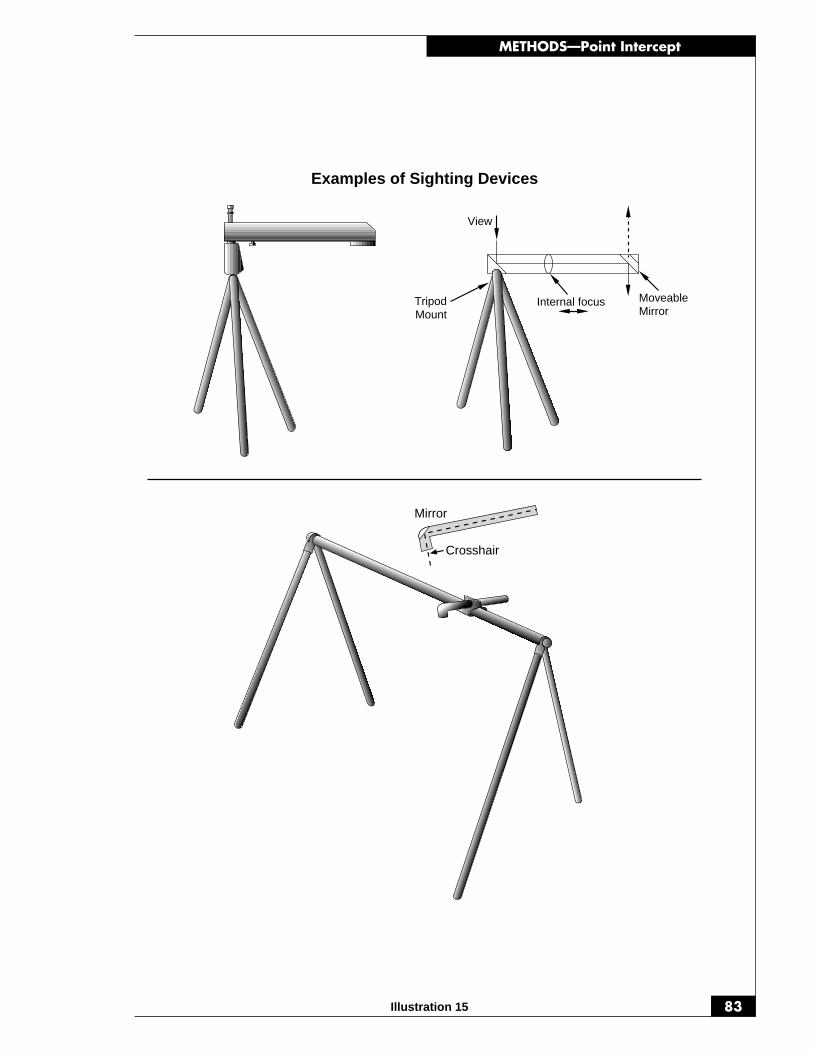
83
METHODS—Point Intercept
Illustration 15
Mirror
Crosshair
Internal focus MoveableMirror
TripodMount
View
Examples of Sighting Devices

METHODS—Point Intercept
84 Illustration 16
Examples of Pin Frames
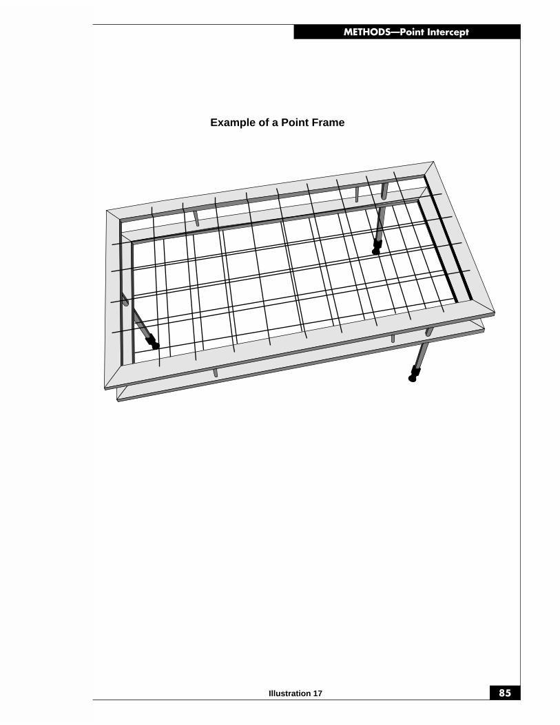
85
METHODS—Point Intercept
Illustration 17
Example of a Point Frame

METHODS—Cover Board
86
H. Cover Board Method
1. General Description The Cover Board method uses a profile board or density boardto estimate the vertical area of a board covered by vegetation from a specified distanceaway. This technique is designed to evaluate changes in the vegetation structure overtime. Quantifying the vegetation structure for statistical comparison was described byNudds (1977). The following vegetation attributes are monitored using this method:
• Vertical cover• Structure
It is important to establish a photo plot (see Section V.A) and take both close-upand general view photographs. This allows the portrayal of resource values andconditions and furnishes visual evidence of vegetation and soil changes over time.
2. Areas of Use This method is applicable to a wide variety of vegetation types. It shouldbe used with those that show potential for changes, such as woody riparian vegetation.
3. Advantages and Limitations The Cover Board technique is a fast and easily dupli-cated procedure. The size of the board can be modified to meet the purpose of the study.
4. Equipment The following equipment is needed (see also the equipment listed inSection V.A, page 31, for the establishment of the photo plot):
• Study Location and Documentation Data form (Appendix A)• Cover Board Method forms (see Illustrations 18 and 19)• Cover board (see Illustration 20)• One stake: 3/4- or 1-inch angle iron not less than 16 inches long• Hammer• Permanent yellow or orange spray paint• Compass• Steel post and driver
5. Training The accuracy of the data depends on the training and ability of theexaminers. They must receive adequate and consistent training in laying outtransects. A minimum of training is needed to make sure the examiners under-stand how to position the cover board and estimate percent cover. Examinersmust also be able to identify plant species if estimates are to be made be species.
6. Establishing Studies Careful establishment of studies is a critical element inobtaining meaningful data (see Section III).
a Site Selection The most important factor in obtaining usable data is selectingrepresentative areas (critical or key areas) in which to run the study (see SectionII.D). Study sites should be located within a single plant community within asingle ecological site. Transects and sampling points need to be randomlylocated within the critical or key areas (see Section III).
b Pilot Studies Collect data on several pilot studies to determine the number ofsamples (transects or observation points) and the number and size of quadratsneeded to collect a statistically valid sample (see Section III.B.8).

87
METHODS—Cover Board
c Number of Transects Establish the minimum number of transects to achieve thedesired level of precision for the key species in each study site (see Section III.B).
d Study Layout Data can be collected using either the baseline or linear studydesigns described in Section III.A.2 beginning on page 8. The linear techniqueis the most often used procedure.
(1) Linear transect
(a) Determine the transect bearing and select a prominent distant land-mark such as a peak, rocky point, etc., that can be used as the transectbearing point.
(b) Randomly select an observation point along the transect. The coverboard will be placed 15 feet from this observation point in a randomdirection. One way to select a random direction is by using the secondhand on a standard watch. Look at the watch and note the directionthe second hand is pointing. Another way is to randomly select a threedigit number between 0 and 360 from a random number table torepresent the degrees on a compass (see Appendix D for directionsand a table of random digits). After taking the initial reading, remainat the observation point on the transect and take three additionalreadings at 90-degree angles from the original bearing and at the samedistance (15 feet). Additional observation points can be established atspecified intervals from the initial observation point along the transectbearing. A piece of angle iron or rebar should be placed at eachobservation point for easy relocation.
(c) Be sure to record the bearing from the observation point to each coverboard location on the Cover Board form (see Illustrations 18 and 19).
(2) Center location
(a) An alternative method of establishing a transect is to randomly select acenter point within an area to be sampled. Set angle iron or rebar atfour randomly selected points 15 feet from the center point. Place thecover board at each rebar, facing the center post. Take readings andphotographs of the cover board from the center point. Additionalcenter points can be established as needed.
(b) Be sure to record the bearing and distance to each center pointlocation from the reference post on the Cover Board form (seeIllustrations 18 and 19).
e Reference Post or Point Permanently mark the location of each study with areference post and a study location stake (see beginning of Section III).
f Study Identification Number studies for proper identification to ensure thatthe data collected can be positively associated with specific sites on the ground(see Appendix B).
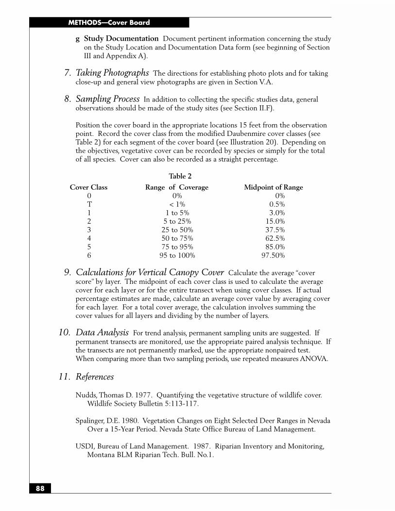
METHODS—Cover Board
88
g Study Documentation Document pertinent information concerning the studyon the Study Location and Documentation Data form (see beginning of SectionIII and Appendix A).
7. Taking Photographs The directions for establishing photo plots and for takingclose-up and general view photographs are given in Section V.A.
8. Sampling Process In addition to collecting the specific studies data, generalobservations should be made of the study sites (see Section II.F).
Position the cover board in the appropriate locations 15 feet from the observationpoint. Record the cover class from the modified Daubenmire cover classes (seeTable 2) for each segment of the cover board (see Illustration 20). Depending onthe objectives, vegetative cover can be recorded by species or simply for the totalof all species. Cover can also be recorded as a straight percentage.
Table 2
Cover Class Range of Coverage Midpoint of Range0 0% 0%T < 1% 0.5%1 1 to 5% 3.0%2 5 to 25% 15.0%3 25 to 50% 37.5%4 50 to 75% 62.5%5 75 to 95% 85.0%6 95 to 100% 97.50%
9. Calculations for Vertical Canopy Cover Calculate the average “coverscore” by layer. The midpoint of each cover class is used to calculate the averagecover for each layer or for the entire transect when using cover classes. If actualpercentage estimates are made, calculate an average cover value by averaging coverfor each layer. For a total cover average, the calculation involves summing thecover values for all layers and dividing by the number of layers.
10. Data Analysis For trend analysis, permanent sampling units are suggested. Ifpermanent transects are monitored, use the appropriate paired analysis technique. Ifthe transects are not permanently marked, use the appropriate nonpaired test.When comparing more than two sampling periods, use repeated measures ANOVA.
11. References
Nudds, Thomas D. 1977. Quantifying the vegetative structure of wildlife cover.Wildlife Society Bulletin 5:113-117.
Spalinger, D.E. 1980. Vegetation Changes on Eight Selected Deer Ranges in NevadaOver a 15-Year Period. Nevada State Office Bureau of Land Management.
USDI, Bureau of Land Management. 1987. Riparian Inventory and Monitoring,Montana BLM Riparian Tech. Bull. No.1.

89
METHODS—Cover Board
Illustration 18
Density Board Location -
Total Average Cover-
Percent Cover
Plot 1 Plot 2 Plot 3 Plot 4 Avg. Cover
5
4
3
2
1
Allotment Name & Number Pasture
Study Number Date Examiner
Page of
Cover Board MethodDensity Board
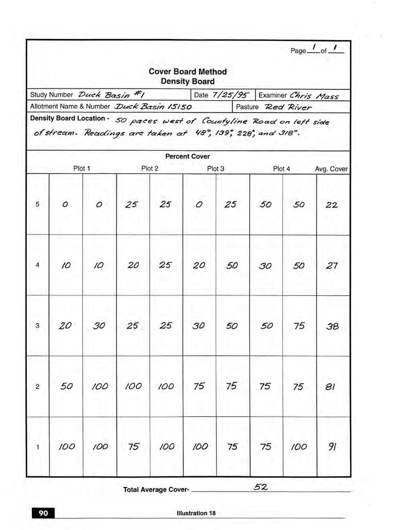

91
METHODS—Cover Board
Illustration 19
Bea
ring
& D
ista
nce
Stu
dy L
ocat
ion
Stu
dy N
umbe
rD
ate
Exa
min
erA
llotm
ent N
ame
& N
umbe
rP
astu
re
Co
ver
Bo
ard
Met
ho
dP
rofi
le B
oar
d
Pag
e
o
f
Cov
er R
eadi
ngs—
Dau
benm
ire C
lass
es1
or P
erce
ntag
es
Spe
cies
Bearing
Total
0.0
- 0.
5m0.
5 -
1.0m
1.0
- 1.
5m1.
5 -
2.0m
Cov
erB
oard
Hei
ghts
ObservationPoints
Com
men
ts:
Bearing
Total
Bearing
Total
Bearing
Total
Ave
rage
1D
aube
nmire
Cla
sses
: 0=
0; 1
=1-
5; 2
=5-
25; 3
=25
-50;
4=
50-7
5; 5
=75
-95;
6=
95-1
00
0.0
- 0.
5m0.
5 -
1.0m
1.0
- 1.
5m1.
5 -
2.0m
0.0
- 0.
5m0.
5 -
1.0m
1.0
- 1.
5m1.
5 -
2.0m
0.0
- 0.
5m0.
5 -
1.0m
1.0
- 1.
5m1.
5 -
2.0m
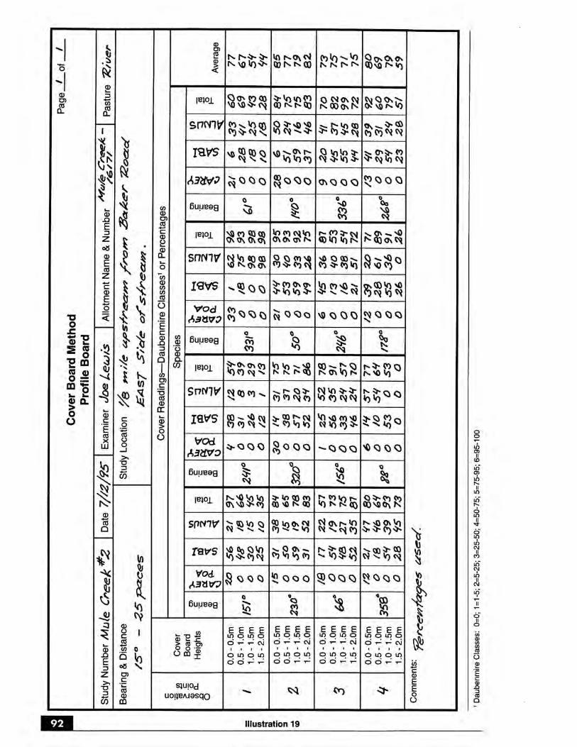

93
METHODS—Cover Board
Illustration 20
hinged inside
hinged
wing nuts
Profile Board Density Board
removablespikes
2'-0"30.48cm
5'-0"2 1/2 m
2'-6"2'-10"
>2
1.5
0.5
2.0
1.0
Examples of Cover Boards
METHODS—Density
94
I. Density Method
1. General Description Density is the number of individuals of a species in agiven unit of area. For rhizomatous and other species for which the delineation ofseparate individual plants is difficult, density can also mean the number of stems,inflorescences, culm groups, or other plant parts per unit area.
2. Areas of Use This method has wide applicability and is suited for use withgrasses, forbs, shrubs, and trees.
3. Advantages and Limitations
a Generally, the density of mature perennial plants is not affected as much byannual variations in precipitation as are other vegetation attributes such ascanopy cover or herbage production.
b Density is a quantifiable and absolute attribute.
c Density is sensitive to changes in the adult population caused by long-termclimatic conditions or resource uses.
d Density provides useful information on seedling emergence, survival, and mortality.
e Sampling is often quick and easy with certain life forms (e.g., trees, shrubs,bunchgrasses).
f Plant communities on the same ecological sites can be compared using densityestimates on specific species or lifeforms.
g Density can be useful in estimating plant responses to management actions.
h It can often be difficult to delineate an individual, especially when sampling sodforming plants (stoloniferous, or rhizomatous plants) and multi-stemmed grassesor closely spaced shrubs. Although in these cases a surrogate plant part (e.g.,upright stems, inflorescences, culm groups) can be counted, the usefulness of suchestimates is limited to the biological significance of changes in these surrogates.
i Sampling may be slow and tedious in dense populations; this also raises the riskof non-sampling errors.
j There is no single quadrat size and shape that will efficiently and adequatelysample all species and life forms. For this reason, density estimations are usuallylimited to one or a few key species.
4. Equipment The following equipment is needed (see also the equipment listed inSection V.A, page 31, for the establishment of the photo plot):
• Study Location and Documentation Data form (see Appendix A)• Density form (see Illustration 21)• Tapes: 50-, 100-, 150-, or 200-meter delineated in centimeters. (Tapes in

95
METHODS—Density
English measurements can be substituted but metric tapes are preferred.) Atleast three tapes are required (one, to be used for constructing quadrats, needonly be as long as the long side of the quadrat; a rope of the desired length canbe substituted for this tape); four are better.
• Meter sticks (or yard sticks if using English measurements). Two are required.• Four stakes: 3/4- or 1-inch angle iron not less than 16 inches long• Hammer• Permanent yellow or orange spray paint• Tally counter (optional)• Compass• Steel post and driver
5. Training As with any monitoring method, adequate training is essential tominimize nonsampling errors.
a Examiners must be able to identify the target plant species.
b For sod-forming grasses and other species for which individual plants might behard to distinguish, written guidelines should be provided on what constitutesan individual unit to be counted.6 This will help to ensure consistency amongexaminers. To assess consistency prior to the study, several examiners should beasked to independently count these units in the same set of quadrats and theresults compared. If relatively consistent results cannot be achieved a differentspecies should be chosen for estimation or a different method selected.
6. Establishing Studies Careful establishment of studies is a critical element inobtaining meaningful data.
a Site Selection The most important factor in obtaining usable data is selectingrepresentative areas (critical or key areas) in which to run the study (see SectionII.D). Study sites should be located within a single plant community within asingle ecological site. Transects and sampling points need to be randomly lo-cated within the critical or key areas (see Section III).
b Pilot Studies Collect data on several pilot studies to determine the number ofsamples (transects or observation points) and the number and size of quadratsneeded to collect a statistically valid sample (see Section III.B.8).
(1) Quadrat size and shape It is vital to choose the quadrat size and shapethat will give the highest statistical precision for the area and key speciesbeing sampled. As a general rule of thumb long, thin quadrats are better
6 Determination of what constitutes a unit to be counted is somewhat arbitrary. For rhizomatous grasses such aswestern wheatgrass (Pascopyrum smithii), each culm group can be visualized as an actual or potential plantunit, as can rooted stoloniferous units of such species as vine mesquite (Panicum obtusum). Mat or sod-forming plants such as blue grama (Bouteloua gracilis) or alkali sacaton (Sporobolus airoides) usually startgrowth as small, distinct clumps, but may spread to plants a meter or more in diameter. As this occurs theytend to fragment into more-or-less separate units, and it is these separate units that should be counted asactual or potential individuals. For rhizomatous or mat-forming forbs, flowering stems may be the unitscounted. The examiner should ensure, however, that a change in the unit chosen is of biological significance,i.e., reflects a real change in the vegetation community. If it has no such significance, then another unit or adifferent species should be chosen. (Alternatively, an attribute other than density can be selected for monitoring.)

METHODS—Density
96
(often very much better) than circles, squares, or shorter and wider quad-rats (Krebs 1989). How narrow the quadrats can be depends upon consid-eration of measurement errors due to edge effect, but these problems canbe largely overcome by incorporating rules for determining whether a plantfalls inside or outside a quadrat (discussed in more detail under SamplingProcess below).
(a) Subjectively place quadrats7 of a certain size and shape in areas withlarge numbers of the target plant species. See how many plants fall intothe quadrat and ask if this is too many to count. See what kind ofproblems there might be with edge effect: when individuals fall on ornear one of the long edges of the quadrat, will it be difficult for examin-ers to make consistent calls as to whether these individuals are in or outof the quadrat? See if there is a tendency to get more plants in rectan-gular quadrats when they are run one way as opposed to another.
(b) Determine the standard deviations of those quadrat sizes and shapesdeemed to be practical from the subjective examination describedabove (see Section III.B.8.b).
(c) Choose the quadrat size and shape with the smallest standard deviation.
(2) Direction of quadrats Determine if there is an environmental gradientaffecting the density of the target species in the key area. Examples of suchgradients are elevation and moisture. If there is a gradient, the studyshould be set up so that the long side of each quadrat is placed perpendicu-lar to this gradient. This ensures that there is more variability within eachquadrat than there is between quadrats.
Subjectively placing quadrats in different directions as described under6.b.(1)(a) above can assist in making this determination. For example, ifquadrats laid out with the long side going north-south tend to have no orfewer plants of the key species than quadrats with the long side going east-west, the east-west position should be selected.
c Study Layout Data can be collected using the baseline, macroplot or linearstudy designs described in Section III.A.2 beginning on page 8. The macroplottechnique is the recommended procedure.
d Reference Post or Point Permanently mark the location of each study with areference post and a study location stake (see beginning of Section III).
e Study Identification Number macroplots for proper identification to ensure
7 Note that it is not necessary to construct an actual frame for the quadrats used. It is sufficient to delineatequadrats using a combination of tape measures and meter (or yard) sticks. For example, a 5 m x 0.25 mquadrat can be constructed by selecting a 5 m interval along a meter tape, placing two 1-meter sticks perpen-dicular to the tape at both ends of the interval (with their zero points at the tape), and laying another tape orrope across these two sticks at their 0.25 m points. This then circumscribes a quadrat of the desired size andshape. Alternately place a meter stick perpendicular to the tape at one end of the interval. The meter stick isthen moved slowly up the interval and all plants of the species occurring within the first 0.25 m of the meterstick recorded until the end of the interval is reached.
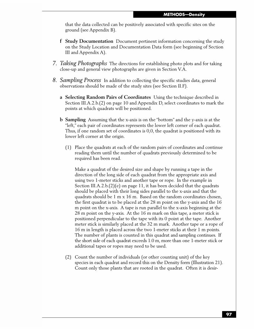
97
METHODS—Density
that the data collected can be positively associated with specific sites on theground (see Appendix B).
f Study Documentation Document pertinent information concerning the studyon the Study Location and Documentation Data form (see beginning of SectionIII and Appendix A).
7. Taking Photographs The directions for establishing photo plots and for takingclose-up and general view photographs are given in Section V.A.
8. Sampling Process In addition to collecting the specific studies data, generalobservations should be made of the study sites (see Section II.F).
a Selecting Random Pairs of Coordinates Using the technique described inSection III.A.2.b.(2) on page 10 and Appendix D, select coordinates to mark thepoints at which quadrats will be positioned.
b Sampling Assuming that the x-axis is on the “bottom” and the y-axis is at the“left,” each pair of coordinates represents the lower left corner of each quadrat.Thus, if one random set of coordinates is 0,0, the quadrat is positioned with itslower left corner at the origin.
(1) Place the quadrats at each of the random pairs of coordinates and continuereading them until the number of quadrats previously determined to berequired has been read.
Make a quadrat of the desired size and shape by running a tape in thedirection of the long side of each quadrat from the appropriate axis andusing two 1-meter sticks and another tape or rope. In the example inSection III.A.2.b.(2)(e) on page 11, it has been decided that the quadratsshould be placed with their long sides parallel to the x-axis and that thequadrats should be 1 m x 16 m. Based on the random coordinates chosen,the first quadrat is to be placed at the 28 m point on the y-axis and the 16m point on the x-axis. A tape is run parallel to the x-axis beginning at the28 m point on the y-axis. At the 16 m mark on this tape, a meter stick ispositioned perpendicular to the tape with its 0 point at the tape. Anothermeter stick is similarly placed at the 32 m mark. Another tape or a rope of16 m in length is placed across the two 1-meter sticks at their 1 m points.The number of plants is counted in this quadrat and sampling continues. Ifthe short side of each quadrat exceeds 1.0 m, more than one 1-meter stick oradditional tapes or ropes may need to be used.
(2) Count the number of individuals (or other counting unit) of the keyspecies in each quadrat and record this on the Density form (Illustration 21).Count only those plants that are rooted in the quadrat. Often it is desir-

METHODS—Density
98
able to make separate counts for different size or age classes of the keyspecies. This is particularly true for seedlings, many of which may notsurvive to the next sampling period.
(a) To eliminate measurement error due to edge effects, it is helpful tohave rules for determining whether an individual plant that fallsexactly on the edge of a quadrat is considered inside or outside thequadrat.
(b) A good rule to follow is to count those individuals falling on the leftand top edges of the quadrat as being inside the quadrat and thoseindividuals falling on the right and bottom edges of the quadrat asbeing outside the quadrat. Make sure that all observers follow thesame set of rules.
9. Calculations Make the calculations and record the results on the Density form(see Illustration 21).
a Average Density per Quadrat Calculate the estimated average density perquadrat for each size/age class by dividing the total number of plants counted inthe sample for each size/age class by the number of quadrats in the sample. Ifmore than one key species is counted, this process is done separately for eachspecies. For example, a sample of 40 quadrats yields a total of 177 individualmature plants of key species Y. The estimated average density of mature plantsper quadrat is therefore 177/40 = 4.4 plants/quadrat.
b Total Density of Macroplot Calculate the estimated total density of themacroplot by multiplying the average density per quadrat by the total numberof possible quadrats in the macroplot. If more than one key species is counted,this process is done separately for each key species. Say the macroplot in theexample given in 9.a above is 40 m x 80 m and the quadrat size is 1.0 m x 16 m.There are 200 possible nonoverlapping quadrat placements in a macroplot ofthis size (40/1 = 40 along one axis and 80/16 = 5 along the other; 40 x 5 = 200possible quadrats). The estimate of the total density of the macroplot is there-fore 4.4 mature plants/quadrat x 200 quadrats = 880 mature plants.
10. Data Analysis and Interpretation Data analysis is straightforward. Confi-dence intervals should be constructed around each of the estimates of averagedensity per quadrat (hereafter referred to simply as “average”) and total macroplotdensity for each year. The averages of two years should be compared by using a ttest (for independent samples). Averages of three or more years can be comparedby an analysis of variance. See Technical Reference, Measuring & Monitoring PlantPopulations.
11. References
Krebs, C.J. 1989. Ecological methodology. Harper & Row, New York. This bookdiscusses the superiority of long, thin quadrats over circular and square quadrats,as well as the potential problems of edge effect.

99
METHODS—Density
Salzer, D. 1994. An introduction to sampling and sampling design for vegetationmonitoring. Unpublished papers prepared for Bureau of Land ManagementTraining Course 1730-5. BLM Training Center, Phoenix, Arizona. These papers,together with material prepared for a class exercise, present the basic conceptsof the Density Method. The Density Method is in rather widespread use inThe Nature Conservancy and, increasingly, by the Bureau of Land Manage-ment and the Forest Service, particularly as a means of estimating numbers ofspecial status plant species.

METHODS—Density
100 Illustration 21
Stu
dy N
umbe
rD
ate
Exa
min
erA
llotm
ent N
ame
& N
umbe
rP
astu
reP
lot S
ize
Den
sity
Pag
e
o
f
Plo
t1
23
45
67
89
10To
tal
Stu
dy L
ocat
ion
See
dlin
gS
eedl
ing
Mat
ure
See
dlin
gM
atur
eS
eedl
ing
Mat
ure
See
dlin
gM
atur
eS
eedl
ing
Mat
ure
See
dlin
gM
atur
eM
atur
eS
eedl
ing
See
dlin
gM
atur
eM
atur
eS
eedl
ing
Mat
ure
See
dlin
gP
lant
Spe
cies
Coo
rdin
ates
Mat
ure

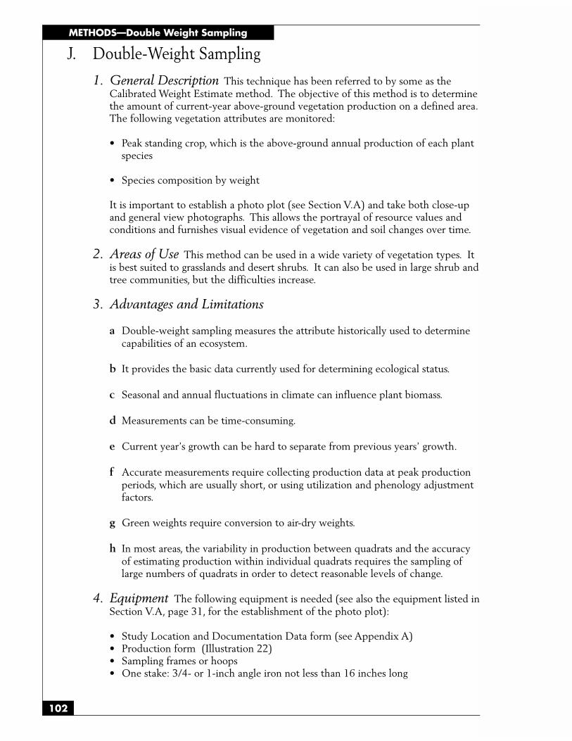
METHODS—Double Weight Sampling
102
J. Double-Weight Sampling
1. General Description This technique has been referred to by some as theCalibrated Weight Estimate method. The objective of this method is to determinethe amount of current-year above-ground vegetation production on a defined area.The following vegetation attributes are monitored:
• Peak standing crop, which is the above-ground annual production of each plantspecies
• Species composition by weight
It is important to establish a photo plot (see Section V.A) and take both close-upand general view photographs. This allows the portrayal of resource values andconditions and furnishes visual evidence of vegetation and soil changes over time.
2. Areas of Use This method can be used in a wide variety of vegetation types. Itis best suited to grasslands and desert shrubs. It can also be used in large shrub andtree communities, but the difficulties increase.
3. Advantages and Limitations
a Double-weight sampling measures the attribute historically used to determinecapabilities of an ecosystem.
b It provides the basic data currently used for determining ecological status.
c Seasonal and annual fluctuations in climate can influence plant biomass.
d Measurements can be time-consuming.
e Current year’s growth can be hard to separate from previous years’ growth.
f Accurate measurements require collecting production data at peak productionperiods, which are usually short, or using utilization and phenology adjustmentfactors.
g Green weights require conversion to air-dry weights.
h In most areas, the variability in production between quadrats and the accuracyof estimating production within individual quadrats requires the sampling oflarge numbers of quadrats in order to detect reasonable levels of change.
4. Equipment The following equipment is needed (see also the equipment listed inSection V.A, page 31, for the establishment of the photo plot):
• Study Location and Documentation Data form (see Appendix A)• Production form (Illustration 22)• Sampling frames or hoops• One stake: 3/4- or 1-inch angle iron not less than 16 inches long

103
METHODS—Double Weight Sampling
• Herbage Yield Tables for Trees by Height, DBH, or Canopy• Clippers• Paper bags• Kilogram and gram spring-loaded scales with clip• Tree diameter measuring tape• Steel post & driver• Oven for drying vegetation• Air-dry weight conversion tables• Rubber bands• Pin flags• Compass
5. Training The accuracy of the data depends on the training and ability of theexaminers. Examiners must be able to identify plant species and determine currentyear’s growth.
6. Establishing Studies Careful establishment of studies is a critical element inobtaining meaningful data (see Section III).
a Site Selection The most important factor in obtaining usable data is selectingrepresentative areas (critical or key areas) in which to run the study (see SectionII.D). Study sites should be located within a single plant community within asingle ecological site. Transects and sampling points need to be randomlylocated within the critical or key areas (see Section III).
(1) The number of quadrats selected depends on the purpose for which theestimates are to be used, uniformity of the vegetation, and other factors(see Section III.B for Statistical Considerations).
(2) The size and shape of quadrats must be adapted to the vegetationcommunity to be sampled (see Section III.B.6).
b Pilot Studies Collect data on several pilot studies to determine the number ofsamples (transects or observation points) and the number and size of quadratsneeded to collect a statistically valid sample (see Section III.B.8).
c Study Layout Production data can be collected using either the baseline,macroplot or linear study designs described in Section III.A.2 beginning onpage 8. The linear technique is the one most often used.
d Number of Transects Establish the minimum number of transects to achieve thedesired level of precision for the key species in each study site (see Section III.B).
e Reference Post or Point Permanently mark the location of each study with areference post and a study location stake (see beginning of Section III).
f Study Identification Number studies for proper identification to ensure thatthe data collected can be positively associated with specific sites on the ground(see Appendix B).

METHODS—Double Weight Sampling
104
g Study and Documentation Document pertinent information concerning thestudy on the Study Location and Documentation Data form (see beginning ofSection III and Appendix A).
7. Taking Photographs The directions for establishing photo plots and for takingclose-up and general view photographs are given in Section V.A.
8. Weight Units Double sampling requires the establishment of a weight unit foreach species occurring in the area to be sampled. All weight units are based oncurrent year’s growth.
a Procedures For Establishing Weight Units:
(1) Decide on a weight unit that is appropriate for each species. A weight unitcould be an entire plant, a group of plants, or an easily identifiable portionof a plant, and can be measured in either pounds or grams.
(2) Visually select a representative weight unit.
(3) Harvest and weigh the plant material to determine the actual weight of theweight unit.
(4) Maintain proficiency in estimating by periodically harvesting and weighingto check estimates of production.
b Estimating Production of a Single Quadrat:
(1) Estimate production by counting the weight units of each species in thequadrat.
(2) Convert weight units for each species to grams or pounds.
(3) Harvest and weigh each species to check estimate of production.
(4) Repeat the process until proficiency is attained.
(5) Periodically repeat the process to maintain proficiency in estimating.
(6) Keep the harvested material, when necessary, for air-drying and weighing toconvert from green weights to air-dry weights.
c Alternate Method of Establishing Weight Units:
(1) Decide on a weight unit that is appropriate for each species. A weight unitcould be an entire plant, a group of plants, or an easily identifiable portionof a plant, and can be measured in either pounds or grams.
(2) Visually select a representative weight unit.
(3) Instead of weighing the material, save it by securing it with rubber bands soportions are not lost.
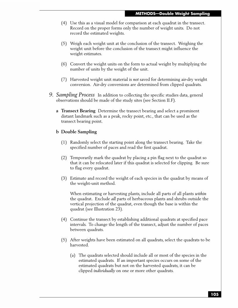
105
METHODS—Double Weight Sampling
(4) Use this as a visual model for comparison at each quadrat in the transect.Record on the proper forms only the number of weight units. Do notrecord the estimated weights.
(5) Weigh each weight unit at the conclusion of the transect. Weighing theweight unit before the conclusion of the transect might influence theweight estimates.
(6) Convert the weight units on the form to actual weight by multiplying thenumber of units by the weight of the unit.
(7) Harvested weight unit material is not saved for determining air-dry weightconversion. Air-dry conversions are determined from clipped quadrats.
9. Sampling Process In addition to collecting the specific studies data, generalobservations should be made of the study sites (see Section II.F).
a Transect Bearing Determine the transect bearing and select a prominentdistant landmark such as a peak, rocky point, etc., that can be used as thetransect bearing point.
b Double Sampling
(1) Randomly select the starting point along the transect bearing. Take thespecified number of paces and read the first quadrat.
(2) Temporarily mark the quadrat by placing a pin flag next to the quadrat sothat it can be relocated later if this quadrat is selected for clipping. Be sureto flag every quadrat.
(3) Estimate and record the weight of each species in the quadrat by means ofthe weight-unit method.
When estimating or harvesting plants, include all parts of all plants withinthe quadrat. Exclude all parts of herbaceous plants and shrubs outside thevertical projection of the quadrat, even though the base is within thequadrat (see Illustration 23).
(4) Continue the transect by establishing additional quadrats at specified paceintervals. To change the length of the transect, adjust the number of pacesbetween quadrats.
(5) After weights have been estimated on all quadrats, select the quadrats to beharvested.
(a) The quadrats selected should include all or most of the species in theestimated quadrats. If an important species occurs on some of theestimated quadrats but not on the harvested quadrats, it can beclipped individually on one or more other quadrats.

METHODS—Double Weight Sampling
106
(b) The number of quadrats harvested depends on the number estimated.At least one quadrat should be harvested for each seven estimated toadequately correct the estimates (see table 3).
Table 3
Number of quadrats Minimum Number ofEstimated Quadrats to be Weighed
1 - 7 18 - 14 2
14 - 21 322 - 28 429 - 35 536 - 42 6
(6) Harvest, weigh, and record the weight of each species in the quadratsselected for harvesting. Harvest all herbaceous plants originating in thequadrat at ground level. On rangeland, harvest all of the current leaf, twig,and fruit production of woody plants located in the quadrats. On nativepasture and grazable woodland, harvest the current leaf, twig, and fruitproduction of woody plants within the plot up to a height of 4 1/2 feetabove the ground. For further clarification see Illustration 23.
(7) Correct estimated weights by dividing the harvested weight of each speciesby the estimated weight for the corresponding species on the harvestedquadrats. This factor is used to correct the estimates for that species ineach quadrat. A factor of more than 1.0 indicates that the estimate is toolow. A factor lower than 1.0 indicates that the estimate is too high.
After quadrats are estimated and harvested and correction factors forestimates are computed, air-dry percentages are determined by air-dryingthe harvested materials or by selecting the appropriate factor from an air-dry percentage table. Values for each species are then converted to air-drypound per acre or kilograms per hectare for all quadrats. Average weightand percentage composition can then be computed for the sample area.
10. Calculations The weights collected for each species per quadrat placement arerecorded on the Production form (see Illustration 22).
a Record estimated weights for each species occurring in each quadrat in theappropriate column (Estimated or Clipped Weight sections of the form.)
b Quadrats that were harvested are circled. The estimate weights for thesequadrats are totaled and shown in column 4. The total harvested weights areshown in column 5. Harvested weights for each quadrat for each species arenot shown on the form, only the total for each species.
c Column 6 is the actual dry weight for each species from the quadrats that wereclipped.
107
METHODS—Double Weight Sampling
d The Quadrat Correction Factor (QCF)column 7 is calculated by dividingcolumn 5 by column 4.
f Column 8 is determined by dividing the dry weight by the green weight. In theexample shown on Illustration 22, the clipped weights were not air dried; thepercent dry weights shown in column 8 were taken from the dry weight conver-sion table.
g The total estimated weights for each species for the entire transect are shown incolumn 9.
h The average yield (column 10) is determined by multiplying the Total Esti-mated Weight of each species (column 9) times the Quadrat Correction Factor(column 7) to adjust for the error in estimating weights and then multiplyingthat times the percent dry weight (column 8) to determine the adjusted dryweight or the Average Yield (column 10).
i The Average Yield for each species (column 10) is totaled at the bottom of theform for the composition totals.
j Percent Composition (column 11) is calculated by dividing the average yield foreach species (column 10) by the composition totals.
k If peak standing crop is collected in grams, it can be easily converted to poundsper acres if the total area sampled is a multiple of 9.6 ft2.
Use table 4 to convert grams to pounds per acre:
Table 4 (# of plots x size = total area)
(10 x 0.96 = 9.6 ft2) multiply grams times 10.0 = pounds per acre(10 x 1.92 = 19.2 ft2) multiply grams times 5.0 = pounds per acre(10 x 2.40 = 24.0 ft2) multiply grams times 4.0 = pounds per acre(10 x 4.80 = 48.0 ft2) multiply grams times 2.0 = pounds per acre(10 x 9.60 = 96.0 ft2) multiply grams times 1.0 = pounds per acre(10 x 96.0 = 960.0 ft2) multiply grams times 0.1 = pounds per acre
11. Data Analysis This technique involves destructive sampling (clipped plots), sopermanent transects or quadrats are not recommended. Since the transects are notpermanently marked, use the appropriate nonpaired test. When comparing morethan two sampling periods, use ANOVA.
12. References
Cook, C. Wayne and James Stubbendieck, 1986. Range Research: Basic Problemsand Techniques. Society for Range Management. Denver, CO.
Laycock, W.A. 1987. Setting Objectives and Picking Appropriate Methods forMonitoring Vegetation on Rangelands. Rangeland Monitoring WorkshopProceedings. U.S. Department of Interior. Bureau of Land Management.Golden, CO.
Revised 2/97

METHODS—Double Weight Sampling
108
Pechanec, J.F. and G.D. Pickford. 1937. A weight-estimate method for the deter-mination of range or pasture production. J. Amer. Soc. Agron. 29:894-904.
Riser, Paul G. 1984. Methods for Inventory and Monitoring of Vegetation, Litter,and Soil Surface Condition. Developing Strategies for Rangeland Monitoring.National Research Council National Academy of Sciences.
USDA, Soil Conservation Service. 1976. National Range Handbook. 154 p.
USDI, Bureau of Land Management. 1984 (rev. 1990). National Range Handbook4410-1. Washington, D. C.
Van Dyne, George M., W.G. Vogel, and H.G. Fisser. 1963. Influence of small plotsize and shape on range herbage production estimates. Ecology 44:746-759.

109
METHODS—Double Weight Sampling
Illustration 22
Pla
ntE
stim
ated
or
Clip
ped
Wei
ght P
er S
peci
esW
t Clip
ped
Plo
tsQ
CF
%D
ryW
t All
Avg
Pct
Pla
nt N
ame
Sym
bol
(Circ
le P
lots
that
are
Clip
ped)
(3)
Est
Clip
Dry
Wt
Plo
tsY
ield
Com
p
(1)
(2)
P-1
P-2
P-3
P-4
P-5
P-6
P-7
P-8
P-9
P-1
0(4
)(5
)(6
)(7
)(8
)(9
)(1
0)(1
1)
Pag
e
o
f
Stu
dy N
umbe
rD
ate
Exa
min
erA
llotm
ent N
ame
& N
umbe
rP
astu
re
Pro
du
ctio
n
Tran
sect
Loc
atio
nQ
uadr
at S
ize
Tran
sect
Bea
ring
Not
es (
use
othe
r si
de o
r an
othe
r pa
ge)
Tota
ls
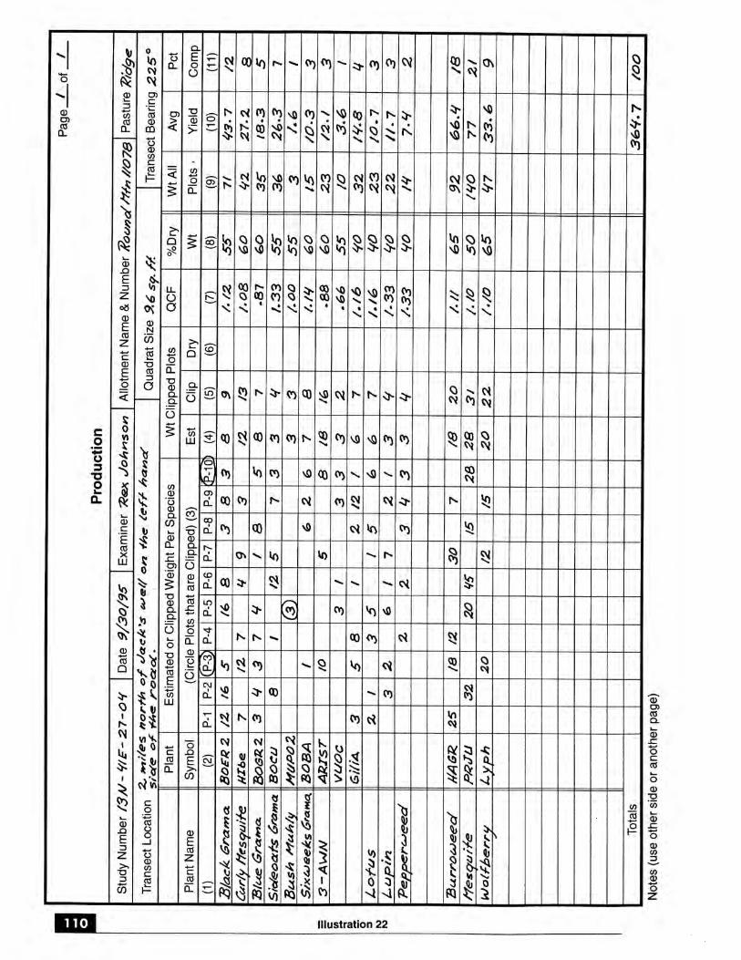

111
METHODS—Double Weight Sampling
Illustration 23
Record weightsof all plants withinthe vertical projectionof the quadrateven though thebase is not withinthe quadrat.
Do not record weights of portions of plants outside the verticalprojection of the quadrat even though the base is within the quadrat
Weight Estimate Quadrat

METHODS—Harvest
112
K. Harvest Method
1. General Description The concept of this method is to determine the amountof current-year above-ground vegetation production on a defined area. Thefollowing vegetation attributes are monitored:
• Peak standing crop, which is the above-ground annual production of each plantspecies
• Species composition by weight
It is important to establish a photo plot (see Section V.A) and take both close-upand general view photographs. This allows the portrayal of resource values andconditions and furnishes visual evidence of vegetation and soil changes over time.
2. Areas of Use This method can be used in a wide variety of vegetation types. Itis best suited for grasslands and desert shrubs. It is not well suited to large shruband tree communities.
3. Advantages and Limitations
a The harvest method measures the attribute historically used to determine thecapabilities of an ecosystem.
b It provides the basic data currently used for determining ecological status.
c Seasonal and annual fluctuations in climate can influence plant biomass.
d Measurements can be time-consuming.
e Current year’s growth can be hard to separate from previous years’ growth.
f Accurate measurements require collecting production data at peak productionperiods which, are usually short, or using utilization and phenology adjustmentfactors.
g Green weights require conversion to air-dry weights.
h In most areas, the variability in production between quadrats requires thesampling of large numbers of quadrats in order to detect reasonable levels ofchange.
4. Equipment The following equipment is needed (see also the equipment listed inSection V.A, page 31, for the establishment of the photo plot):
• Study Location and Documentation Data form (see Appendix A)• Production form (Illustration 22, page 109)• Sampling frames or hoops• One stake: 3/4- or 1-inch angle iron not less than 16 inches long• Herbage Yield Tables for Trees by Height, DBH, or Canopy

113
METHODS—Harvest
• Clippers• Paper bags• Kilogram and gram spring-loaded scales with clip• Tree diameter measuring tape• Steel post and driver• Oven for drying vegetation• Air-dry weight conversion tables• Rubber bands• Compass
5. Training The accuracy of the measurement depends on the training and abilityof the examiners. Examiners must be able to identify plant species and determinecurrent year’s growth.
6. Establishing Studies Careful establishment of studies is a critical element inobtaining meaningful data (see Section III).
a Site Selection The most important factor in obtaining usable data is selectingrepresentative areas (critical or key areas) in which to run the study (see SectionII.D). Study sites should be located within a single plant community within asingle ecological site. Transects and sampling points need to be randomlylocated within the critical or key areas (see Section III).
(1) Select transects at random (see Section III.B. 2).
(2) The number of quadrats selected depends on the purpose for which theestimates are to be used, uniformity of the vegetation, and other factors(see Section III.B for Statistical considerations.)
(3) Adapt the size and shape of quadrats to the vegetation community to besampled (see Section III.B.6).
b Pilot Studies Collect data on several pilot studies to determine the number ofsamples (transects or observation points) and the number and size of quadratsneeded to collect a statistically valid sample (see Section III.B.8).
c Study Layout Production data can be collected using either the baseline,macroplot, or linear study designs described in Section III.A.2 beginning onpage 8. The linear technique is the one most often used.
d Reference Post or Point Permanently mark the location of each study with areference post and a study location stake (see beginning of Section III).
e Study Identification Number studies for proper identification to ensure thatthe data collected can be positively associated with specific sites on the ground(Appendix B).
f Study Documentation Document pertinent information concerning the studyon the Study Location and Documentation Data form (see beginning of SectionIII and Appendix A).
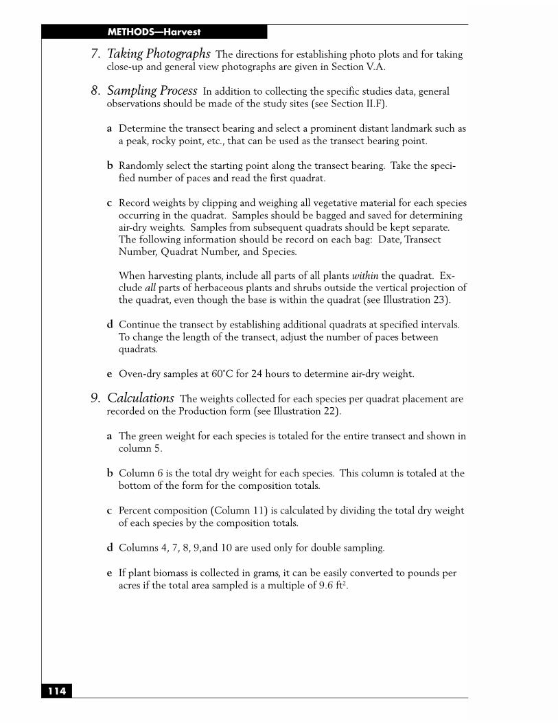
METHODS—Harvest
114
7. Taking Photographs The directions for establishing photo plots and for takingclose-up and general view photographs are given in Section V.A.
8. Sampling Process In addition to collecting the specific studies data, generalobservations should be made of the study sites (see Section II.F).
a Determine the transect bearing and select a prominent distant landmark such asa peak, rocky point, etc., that can be used as the transect bearing point.
b Randomly select the starting point along the transect bearing. Take the speci-fied number of paces and read the first quadrat.
c Record weights by clipping and weighing all vegetative material for each speciesoccurring in the quadrat. Samples should be bagged and saved for determiningair-dry weights. Samples from subsequent quadrats should be kept separate.The following information should be record on each bag: Date, TransectNumber, Quadrat Number, and Species.
When harvesting plants, include all parts of all plants within the quadrat. Ex-clude all parts of herbaceous plants and shrubs outside the vertical projection ofthe quadrat, even though the base is within the quadrat (see Illustration 23).
d Continue the transect by establishing additional quadrats at specified intervals.To change the length of the transect, adjust the number of paces betweenquadrats.
e Oven-dry samples at 60˚C for 24 hours to determine air-dry weight.
9. Calculations The weights collected for each species per quadrat placement arerecorded on the Production form (see Illustration 22).
a The green weight for each species is totaled for the entire transect and shown incolumn 5.
b Column 6 is the total dry weight for each species. This column is totaled at thebottom of the form for the composition totals.
c Percent composition (Column 11) is calculated by dividing the total dry weightof each species by the composition totals.
d Columns 4, 7, 8, 9,and 10 are used only for double sampling.
e If plant biomass is collected in grams, it can be easily converted to pounds peracres if the total area sampled is a multiple of 9.6 ft2.

115
METHODS—Harvest
Use the following table to convert grams to pounds per acre:
Table 5 (# of plots x size = total area)
(10 x 0.96 = 9.6 ft2) multiply grams times 10.0 = pounds per acre(10 x 1.92 = 19.2 ft2) multiply grams times 5.0 = pounds per acre(10 x 2.40 = 24.0 ft2) multiply grams times 4.0 = pounds per acre(10 x 4.80 = 48.0 ft2) multiply grams times 2.0 = pounds per acre(10 x 9.60 = 96.0 ft2) multiply grams times 1.0 = pounds per acre(10 x 96.0 = 960.0 ft2) multiply grams times 0.1 = pounds per acre
10. Data Analysis This technique involves destructive sampling (clipped plots), sopermanent transects or quadrats are not recommended. Since the transects are notpermanently marked, use the appropriate nonpaired test. When comparing morethan two sampling periods, use ANOVA.
11. References
Cook, C. Wayne and James Stubbendieck, 1986. Range Research: Basic Problemsand Techniques. Society for Range Management. Denver, CO.
Laycock, W.A. 1987. Setting Objectives and Picking Appropriate Methods forMonitoring Vegetation on Rangelands. Rangeland Monitoring WorkshopProceedings. U.S. Department of Interior. Bureau of Land Management.Golden, CO.
Pechanec, J.F. and G.D. Pickford. 1937. A weight-estimate method for the deter-mination of range or pasture production. J. Amer. Soc. Agron. 29:894-904.
Riser, Paul G. 1984. Methods for Inventory and Monitoring of Vegetation, Litter,and Soil Surface Condition. Developing Strategies for Rangeland Monitoring.National Research Council National Academy of Sciences.
USDA, Soil Conservation Service. 1976. National Range Handbook. 154 p.
USDI, Bureau of Land Management. 1984 (rev. 1990). National Range Handbook4410-1. Washington D. C.
Van Dyne, George M., W.G. Vogel, and H.G. Fisser. 1963. Influence of small plotsize and shape on range herbage production estimates. Ecology 44:746-759.
Revised 2/97
METHODS—Comparative Yield
116
L. Comparative Yield Method
1. General Description This method is used to estimate total standing crop orproduction of a site. The total production in a sample quadrat is compared to oneof five reference quadrats; relative ranks are recorded rather than estimating theweight directly.
It is important to establish a photo plot (see Section V.A) and take both close-upand general view photographs. This allows the portrayal of resource values andconditions and furnishes visual evidence of vegetation and soil changes over time.
2. Areas of Use This method works best for herbaceous vegetation but can also beused successfully with small shrubs and half-shrubs. As with most productionestimates, the comparative yield method can be used to compare relative produc-tion between different sites.
3. Advantages and Limitations The advantage of the comparative yieldmethod is that a large sample can be obtained quickly. Total production is evalu-ated, so clipping calibration on a species basis is not needed. The process of develop-ing reference quadrats for ranking purposes reduces both sampling and training time.This technique can be done in conjunction with the frequency, canopy cover, or dryweight rank methods. Identification of individual species is not required.
Large shrub communities are not well suited for this technique. If used in con-junction with other techniques (frequency and dry weight rank), the quadrat sizemay need to be different. This technique can detect only large changes inproduction.
4. Equipment The following equipment is needed (see also the equipment listed inSection V.A, page 31, for the establishment of the photo plot):
• Study Location and Documentation Data form (see Appendix A)• Comparative Yield form (Illustration 24)• Five sampling quadrat frames• Clippers• Paper bags• Kilogram and gram spring-loaded scale with clip• One stake: 3/4- or 1-inch angle iron not less than 16 inches long• Tally counter (optional)• Hammer• Permanent yellow or orange spray paint• Compass• Steel post and driver
5. Training Examiners must calibrate their estimates when sampling situationschange (i.e., different sites, time of day, or season).
6. Establishing Studies Careful establishment of studies is a critical element inobtaining meaningful data. Depending on the objectives, comparative yield datacan be collected on permanent transects or in a random or systematic design.
117
METHODS—Comparative Yield
a Site Selection The most important factor in obtaining usable data is selectingrepresentative areas (critical or key areas) in which to run the study (see SectionII.D). Study sites should be located within a single plant community within asingle ecological site. Transects and sampling points need to be randomlylocated within the critical or key areas (see Section III).
b Pilot Studies Collect data on several pilot studies to determine the number ofsamples (transects or observation points) and the number and size of quadratsneeded to collect a statistically valid sample (see Section III.B.8).
c Selecting Quadrat Size The criteria for selecting the proper size quadrat isthe same as any weight estimate procedure (see Section III.B.6.d).
(1) Determine the proper size quadrat(s) to use by doing preliminary samplingwith different size frames.
(2) Use the same size quadrat throughout a study and for rereading the study.
d Number of Transects Establish one transect on each study site; establish moreif needed.
e Study Layout Production data can be collected using the baseline, macroplot,or linear study designs described in Section III.A.2 beginning on page 8. Thelinear technique is the one most often used.
f Reference Post or Point Permanently mark the location of each study with areference post and a study location stake (see beginning of Section III).
g Study Identification Number studies for proper identification to ensure thatthe data collected can be positively associated with specific sites on the ground(see Appendix B).
h Study Documentation Document pertinent information concerning the studyon the Study Location and Documentation Data form (see beginning of SectionIII and Appendix A).
7. Taking Photographs The directions for establishing photo plots and for takingclose-up and general view photographs are given in Section V.A.
8. Sampling Process In addition to collecting the specific study data, generalobservations should be made of the study sites (see Section II.F).
a A set of reference quadrats must be established. The sample quadrats will becompared and rated back to these reference quadrats. The reference quadratsrepresent the range in dry weight of standing crop that will be commonly foundduring sampling.
METHODS—Comparative Yield
118
(1) Five reference quadrats are subjectively located. References 1 and 5 arelocated first. The first quadrat (reference 1) is placed in a low-yielding areawhich represents the low-yielding situations commonly encountered on thesite (avoid bare or nearly bare quadrats). Reference 5 is determined byplacing a quadrat on a high-yielding area, excluding unusually densepatches of vegetation which would have a rare chance of being sampled.The examiner should make a mental note of the amount of production ineach of the reference quadrats. These references are then clipped andweighed. If the clipped weight in reference 5 is more than five times theweight found in reference 1, then two new sites should be selected asreferences 1 and 5. In establishing the initial reference quadrats, theweight in reference 5 is usually too high and the weight in reference 1 istoo low. Make sure reference 5 does not represent a rare situation. Whenreferences 1 and 5 have been selected, reference 3 is located by placing aframe in an area considered to have a yield halfway between references 1and 5. References 2 and 4 are located the same way by selecting the mid-point yield between references 1 and 3 and references 3 and 5, respectively.
(2) All five reference quadrats are clipped and weighed to compare the refer-ence quadrats to a linear distribution of quadrat weights. This process isrepeated by clipping additional quadrats until the weights of the fivereference quadrats are approximately linear and observers are confident intheir ability to rank quadrats relative to one of the five references. If therankings are not linear, the precision of the method will be reduced. Ifmore than five percent of the quadrats have no production, then a largerquadrat frame should be used.
(3) In areas with less than 500 lb/ac, small quadrats are difficult to evaluate. Inthese situations, larger quadrats should be used or three reference quadratsshould be established instead of five.
b Collecting the Data
(1) Start a transect by randomly locating the first quadrat along the transectbearing.
(2) Read additional quadrats at specified intervals. To change the length of thetransect, increase the number of paces between quadrats.
(3) For each quadrat, compare the total yield in the quadrat to the referencesand record the appropriate rank by dot count tally. It is appropriate toassign intermediate ranks if the yield is at the midpoint between tworeferences. For example, if a quadrat has a yield between references 1 and 2,assign a rank of 1.5. If a quadrat yield greatly exceeds the yield of refer-ence 5, then a higher rank may be estimated. For example, if a quadrat is50% greater than reference 5, a rank of 7 could be recorded. If more thanfive percent of the quadrats are ranked above 5, the references were notproperly selected.
(4) To calibrate the ranks, several quadrats representing each reference shouldbe clipped and weighed independently of the transect. The total yield in

119
METHODS—Comparative Yield
each quadrat is determined without regard to species. Be sure to save allclipped material. The reference quadrats can be used as part of theseclipped quadrats. The more quadrats clipped, the better the calibration.Each distinct sampling period should have a separate calibration. Bags canbe weighed in the field to determine green weight and then saved anddried to determine dry weight (see Section V.J.9.b.(6)). These weights arethen used to determine average weight per reference.
9. Calculations The number of quadrats tallied for each ranking is totaled(Illustration 7, column 2) and multiplied by the ranking (column 1).
Rank x Tally = Weighted ranking
These weighted rankings (column 3) are summed and divided by the number oftotal quadrats. This indicates the average ranking for the site.
___________Total rank___________ = Average ranking for the siteTotal number of quadrats sampled
The average yield may be estimated with a ratio estimate (described below) or aleast-squares regression technique. The ratio estimate is good for quick fieldcalculations, but the least-squares regression should be used for final data analysis.
To use the ratio estimate technique, calculate the average rank and average clippedweight of the harvested quadrats by dividing the total of the clipped rankings and thetotal clipped weight by the number of harvested (clipped) quadrats (column 4 and 5).
____Total of clipped rankings____ = Average rank of clipped quadratsTotal number of clipped quadrats
______Total clipped weight______ = Average weight of clipped quadratsTotal number of clipped quadrats
The average clipped weight is then divided by the average rank to determine theaverage rank interval.
Average weight of clipped quadrats = Average rank interval (ARI)Average rank of clipped quadrats
The average ranking for the site—which is based on the estimated, not clipped,quadrats—is then multiplied by the average rank interval to estimate the averageyield per quadrat for the site.
Average ranking for the site x Average rank interval = Average yield/Quadrat.
The average yield in grams per quadrat obtained above can be converted to eitherpounds/acre or kilograms/hectare.
Use the following table to convert grams to pounds per acre if the total areasampled is a multiple of 9.6 ft2.

METHODS—Comparative Yield
120
Table 6 (# of plots x size = total area)
(10 x 0.96 = 9.6 ft2) multiply grams times 10.0 = pounds per acre(10 x 1.92 = 19.2 ft2) multiply grams times 5.0 = pounds per acre(10 x 2.40 = 24.0 ft2) multiply grams times 4.0 = pounds per acre(10 x 4.80 = 48.0 ft2) multiply grams times 2.0 = pounds per acre(10 x 9.60 = 96.0 ft2) multiply grams times 1.0 = pounds per acre(10 x 96.0 = 960.0 ft2) multiply grams times 0.1 = pounds per acre
To convert to kilograms per hectare, first determine the number of quadrats in ahectare by dividing the number of square meters in a hectare (10,000m2) by thetotal area (in square meters) of the quadrat. Then divide the number of quadratsin a hectare by 1,000 to arrive at the conversion factor used to convert grams perquadrat into kilograms per hectare.
For example, if the quadrat size is 40 X 40 centimeters (0.4 X 0.4 meters), thenthe quadrat area would be 0.4 multiplied by 0.4, or .16m2. The number of quad-rats in a hectare is calculated by dividing 10,000 by .16, which works out to62,500 quadrats per acre. Dividing this number by 1,000 results in the conversionfactor, which is 62.5. The final step is to multiply the average yield per quadratobtained from the final equation above by 62.5 to arrive at kilograms per hectare.
10. Data Analysis For trend analysis, permanent sampling units are suggested. Ifpermanent transects are monitored, use the appropriate paired analysis technique.If the transects are not permanently marked, use the appropriate nonpaired test.When comparing more than two sampling periods, use repeated measures ANOVA.
11. References
Despain, D.W., P.R. Ogden, and E.L. Smith. 1991. Plant frequency sampling formonitoring rangelands. In: G.B. Ruyle, ed. Some Methods for MonitoringRangelands and other Natural Area Vegetation. Extension Report 9043,University of Arizona, College of Agriculture, Tucson, AZ.
Revised 2/97

121
METHODS—Comparative Yield
Illustration 24
Study Location
Notes
Sampled Quadrats Harvested Quadrat
Rank (1) Tally (2) Rank x Tally (3) Clip Rank (4) Clip Weight (5)
0
.5
1
1.5
2
2.5
3
3.5
4
4.5
5
Total
Average
Page of
Comparative Yield
Allotment Name & Number Number of Quadrats Quadrat Size
Study Number Date Examiner Pasture
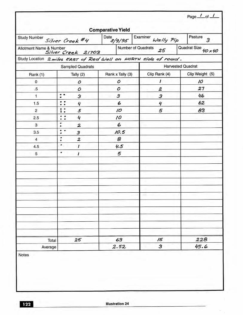
123
METHODS—Visual Obstruction—Robel Pole
M. Visual Obstruction Method - Robel Pole
1. General Description This method is used for determining standing plantbiomass on an area. It has primarily been used to determine the quality of nestingcover for birds on the Great Plains and is commonly referred to as the Robel PoleMethod. This method is applicable to other ecosystems throughout the westernU.S. where height and vertical obstruction of cover are important. The followingvegetation attributes are monitored using this method:
• Vertical cover• Production• Structure
It is important to establish a photo plot (see Section V.A) and take both close-upand general view photographs. This allows the portrayal of resource values andconditions and furnishes visual evidence of vegetation and soil changes over time.
2. Areas of Use The Robel Pole Method is most effective in upland and riparianareas where perennial grasses, forbs, and shrubs less than 4 feet tall are the pre-dominant species.
3. Advantages and Disadvantages Robel Pole measurements are simple,quick, and accurate. This method can be used to monitor height and density ofstanding vegetation over large areas quickly. Statistical reliability improves becausenumerous measurements can be taken in a relatively short time. Limitations of themethod may stem from infrequent application in a variety of rangeland ecosys-tems. While the Robel Pole Method has been used with great success on the GreatPlains, there needs to be more research in a variety of plant communities.
4. Equipment The following equipment is needed (see also the equipment listed inSection V.A, page 31, for the establishment of the photo plot):
• Study Location and Documentation Data form (see Appendix A)• Robel Pole form (Illustration 25)• Cover classes for the area or plant community• Robel pole (Illustration 26)• One stake: 3/4- or 1-inch angle iron not less than 16 inches long• Hammer• Permanent yellow or orange spray paint• Compass• Steel post and driver
5. Training The accuracy of the data depends on the training and ability of theexaminers. They must receive adequate and consistent training in laying outtransects, determining cover classes, and reading the Robel pole.
6. Establishing Studies Careful establishment of studies is a critical element inobtaining meaningful data. Select study sites that are representative of muchlarger areas in terms of similar cover levels.

METHODS—Visual Obstruction—Robel Pole
124
a Site Selection The most important factor in obtaining usable data is selectingrepresentative areas (critical or key areas) in which to run the study (see SectionII.D). Study sites should be located within a single plant community within asingle ecological site. Transects and sampling points need to be randomlylocated within the critical or key areas (see Section III).
b Pilot Studies Collect data on several pilot studies to determine the number ofsamples (transects or observation points) and the number and size of quadratsneeded to collect a statistically valid sample (see Section III.B.8).
c Vertical Cover Classes Establish the number of vertical cover classes andheight limits for each class based on objectives. These cover classes must bedeveloped locally for each ecological site or plant community. The following isan example of cover classes established for upland bird nesting cover on the FortPierre National Grasslands:
Cover Classes Visual Obstruction Height
1 0.0 - 1.92 2.0 - 2.93 3.0 - 3.94 4.0 +
d Number of Transects Establish the minimum number of transects to achieve thedesired level of precision for the key species in each study site (see Section III.B).
e Number of Observation Points The number of observation points willdepend on the objectives, level of precision required, etc.; however, it is recom-mended that a minimum of 50 be read per transect. Additional observationpoints should be read, depending on the pilot study.
f Study Layout Data can be collected using the baseline, macroplot, or linearstudy designs described in Section III.A.2 beginning on page 8. The lineartechnique is the one most often used.
g Reference Post or Point Permanently mark the location of each study with areference post and a study location stake (see beginning of Section III).
h Study Identification Number studies for proper identification to ensure thatthe data collected can be positively associated with specific sites on the ground(see Appendix B).
i Study Documentation Document pertinent information concerning the studyon the Study Location and Documentation Data form (see beginning of SectionIII and Appendix A).
7. Taking Photographs The directions for establishing photo plots and for takingclose-up and general view photographs are given in Section V.A.
125
METHODS—Visual Obstruction—Robel Pole
8. Sampling Process In addition to collecting the specific studies data, generalobservations should be made of the study sites (see Section II.F).
This technique is most effectively accomplished with two individuals.
a Determine the transect bearing and select a prominent distant landmark such asa peak, rocky point, etc., that can be used as the transect bearing point.
b Start a transect by randomly selecting a point along the transect. Two VisualObstruction (VO) measurements are taken at each observation point fromopposite directions along the contour. One examiner holds the Robel pole atthe observation point, while the second examiner holds the end of the cordperpendicular to the transect. The Visual Observation (VO) measurement ismade by determining the highest 1-inch band totally or partially visible andrecording the height on the Robel Pole form (Illustration 25).
c Continue the transect by taking readings at specified intervals along the transectbearing until the transect is complete. The distance between observation pointscan be increased to expand the area sampled.
9. Calculations
a Total the visual obstruction measurements on the Robel Pole form (Illustration 25)for both readings at each observation point and record at the bottom of theform. Add these two totals and divide by the total number of readings. Thiswill yield the average visual obstruction.
b The average height or visual obstruction value can be used to determine thecover class.
10. Production Data from the Robel pole method can be correlated to forageproduction or standing crop. This correlation can be established by clipping andweighing the standing crop within a specified quadrat frame directly in front of theRobel pole after the readings are made. Depending on the vegetation communityapproximately 25 quadrat frames need to be clipped to get a good correlationbetween visual obstruction readings and standing crop. Note that this will be anestimate of standing plant biomass. It will include not only this year’s production,but also herbage remaining from prior years. After the correlation is made be-tween the pole readings and production, the pole can then be used to quicklyestimate production across the entire plant community.
11. Data Interpretation The average Visual Obstruction value can be used todetermine success at meeting objectives. The average Visual Obstruction valuedetermined from the Robel Method form is compared with the cover classes andthe residue levels to determine if overall objectives have been meet.
12. Data Analysis This technique involves destructive sampling (clipped plots), sopermanent transects or quadrats are not recommended. Since the transects are notpermanently marked, use the appropriate nonpaired test. When comparing morethan two sampling periods, use ANOVA.
METHODS—Visual Obstruction—Robel Pole
126
13. References
Robel, R.J., J.N. Briggs, A.D. Dayton, and L.C. Hulbert. 1970. RelationshipsBetween Visual Obstruction Measurements and Weight of Grassland Vegetation,J. Range Manage. 23:295.
Robel, R.J. 1970. Possible Role of Behavior in Regulating Greater PrairieChicken’s Populations, J. Wildlife Manage. Vol 34:306-312.
Snyder, W.D. 1991. Wheat stubble as nesting cover for ring necked pheasants innorthern Colorado. Wildlife Soc. bulletin vol 19(4).
USDA, Forest Service. 1994. Rangeland Analysis and Management TrainingGuide, Rocky Mountain Region USDA Forest Service Denver, Colorado.

127
METHODS—Visual Obstruction—Robel Pole
Illustration 25
1
2
3
4
5
6
7
8
9
10
11
12
13
14
15
16
17
18
19
20
21
22
23
24
25
Total
Grand
Total
Average
Transect #- 1 #- #- #-
Station VO VO VO VO VO VO VO VO
Sampling Interval Study Location
Allotment Name & Number Pasture
Study Number Date Examiner
Robel Pole
Page of
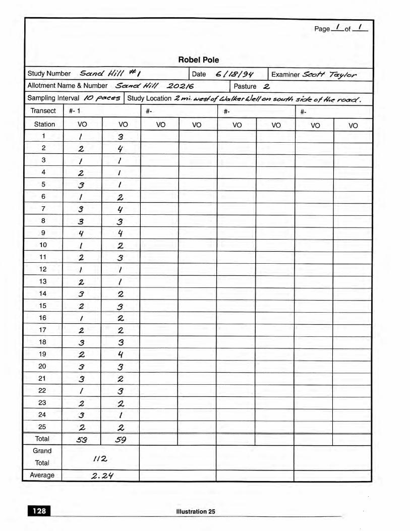
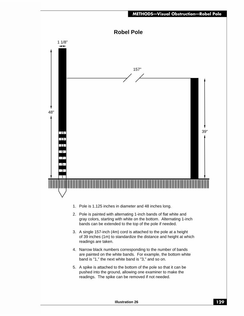
129
METHODS—Visual Obstruction—Robel Pole
Illustration 26
39"15
13
11
9
7
5
3
1
48"
1 1/8"
157"
Robel Pole
Pole is 1.125 inches in diameter and 48 inches long.
Pole is painted with alternating 1-inch bands of flat white and gray colors, starting with white on the bottom. Alternating 1-inchbands can be extended to the top of the pole if needed.
A single 157-inch (4m) cord is attached to the pole at a heightof 39 inches (1m) to standardize the distance and height at whichreadings are taken.
Narrow black numbers corresponding to the number of bandsare painted on the white bands. For example, the bottom white band is "1," the next white band is "3," and so on.
A spike is attached to the bottom of the pole so that it can bepushed into the ground, allowing one examiner to make thereadings. The spike can be removed if not needed.
1.
2.
3.
4.
5.

METHODS—Other
130
N. Other Methods
1. Weight Estimate and Ocular Reconnaissance Methods Both of thesemethods were commonly used to determine forage production prior to the imple-mentation of the Ecological Site Inventory Method. They both involved determin-ing the production on all species, which could then be used to calculate speciescomposition and total production. Although they are no longer widely usedtechniques, written description for completing each can be found in BLM’s Range-land Inventory and Monitoring Supplemental Studies, Technical Reference 4400-5.
2. Community Structure Analysis Method This technique is used by veryfew field offices. It will be moved to BLM’s Technical Reference 4400-5 in afuture revision.
3. Photo Plot Method This technique requires many quadrats for each study sitein order to provide statistically reliable data. Since this technique is very timeconsuming, it is no longer used in most field offices. It will be moved to BLM’sTechnical Reference 4400-5 in a future revision.
131
GLOSSARY
VI. GLOSSARY OF TERMSA
actual use: a report of the actual livestock grazing use certified to be accurate by the per-mittee or lessee. Actual use may be expressed in terms of animal unit months or animalmonths.
allotment: an area of land designated and managed for grazing by livestock. Such an areamay include intermingled private, state, or federal lands used for grazing in conjunctionwith the public lands.
allotment management plan (AMP): a documented program which applies to livestockgrazing on the public lands, prepared by consulting, cooperating, and coordinating withthe permittee(s), lessee(s), or other interested publics.
analysis: (1) a detailed examination of anything complex in order to understand its natureor determine its essential features; or (2) a separating or breaking up of any whole into itscomponent parts for the purpose of examining their nature, function, relationship, etc. Arangeland analysis includes an examination of both biotic (plants, animals, etc.) and abiotic(soils, topography, etc.) attributes of the rangeland.
annual plant: a plant that completes its life cycle and dies in 1 year or less.
animal month: a month’s tenure upon the rangeland by one animal. Animal month is notsynonymous with animal unit month.
animal unit: considered to be one mature cow of approximately 1,000 pounds, either dry orwith calf up to six months of age, or their equivalent, based on a standardized amount offorage consumed.
animal unit month (AUM): the amount of dry forage required by one animal unit for onemonth, based on a forage allowance of 26 pounds per day.
apparent trend: an assessment, using professional judgement, based on a one-time observa-tion. It includes consideration of such factors as plant vigor, abundance of seedlings andyoung plants, accumulation or lack of plant residues on the soil surface, and soil surfacecharacteristics (i.e., crusting, gravel pavement, pedicled plants, and sheet or rill erosion.
available forage: that portion of the forage production that is accessible for use by a speci-fied kind or class of grazing animal.
Bbasal cover (area): the cross-sectional area of the stem or stems of a plant, or all plants in a
stand. Herbaceous and small woody plants are measured at or near the ground level;larger woody plants are measured at breast or other designated height.
biomass: the total amount of living plants and animals above and below ground in an areaat a given time.

GLOSSARY
132
browse: (1) the part of shrubs, half shrubs, woody vines, and trees available for animalconsumption; or (2) to search for or consume browse.
browse plant or browse species: a shrub, half shrub, woody vine, or tree capable of produc-ing shoot, twig, and leaf growth suitable for animal consumption.
Ccanopy cover: the percentage of ground covered by a vertical projection of the outermost
perimeter of the natural spread of foliage of plants. Small openings within the canopy areincluded. Canopy cover is synonymous with crown cover.
class of livestock: the age and/or sex groups of a kind of livestock.
community: an assemblage of populations of plants and/or animals in a common spatialarrangement.
composition: the proportions of various plant species in relation to the total on a given area.It may be expressed in terms of relative cover, relative density, relative weight, etc.
cool season species: plants whose major growth occurs during the late fall, winter and earlyspring.
crown cover: (See canopy cover.)
critical area: an area which should be treated with special consideration because of inherentsite factors, size, location, condition, values, or significant potential conflicts among uses.
D
density: numbers of individuals or stems per unit area (does not equate to any kind of covermeasurement).
Eecological site: a kind of rangeland with a specific potential natural community and specific
physical site characteristics, differing from other kinds of rangeland in its ability to pro-duce vegetation and to respond to management. Ecological sites are defined and de-scribed with soil, species composition, and production emphasis. Ecological site is synony-mous with range site and ecological type (FS).
ecological status: the present state of vegetation of an ecological site in relation to thepotential natural community for the site. Ecological status is independent of use. It is anexpression of the relative degree to which the kinds, proportions, and amounts of plants ina community resemble that of the potential natural community. The four ecologicalstatus classes correspond to 0-25, 26-50, 51-75, or 76-100 percent similarity to the poten-tial natural community and are called early-seral, mid-seral, late-seral, and potential naturalcommunity, respectively.
estimated use: the use made of forage on an area by wildlife, wild horses, wild burros, and/or livestock where actual use data are not available. Estimated use may be expressed interms of animal unit months or animal months.
133
GLOSSARY
evaluation: (1) an examination and judgment concerning the worth, quality, significance,amount, degree, or condition of something; or (2) the systematic process for determiningthe effectiveness of on-the-ground management actions and assessing progress towardmeeting objectives.
Ffoliar cover: the percentage of ground covered by a downward vertical projection of the
aerial portion of plant foliage, excluding small openings in the canopy, Foliar cover isalways less than canopy cover. Total foliar cover of all species may exceed 100 percent.
forage: (1) browse and herbage which is available and can provide food for animals or beharvested for feeding; or (2) to search for or consume forage.
forage production: the weight of forage that is produced within a designated period of timeor a given area. Production may be expressed as green, air dry, or oven dry weight. Theterm may also be modified as to time of production such as annual, current year, orseasonal forage production.
forb: (1) any herbaceous plant other than those in the Gramineae (true grasses),Cyperaceae (sedges), and Juncaceae (rushes) families—i.e., any nongrass-like plant havinglittle or no woody material on it; or (2) a broadleaved flowering plant whose above-ground stem does not become woody and persistent.
forestland: land on which the vegetation is dominated by trees. Lands are classified forest-land if the trees now present will provide 25 percent or greater canopy cover at maturity.Lands not presently forestland that were originally or could become forested throughnatural succession may be classified as potential natural forestland.
frequency: a quantitative expression of the presence or absence of individuals of a species ina population. It is defined as the percentage of occurrence of a species in a series ofsamples of uniform size.
Ggoal: the desired state or condition that a resource management policy or program is de-
signed to achieve. A goal is usually not quantifiable and may not have a specific date bywhich it is to be completed. Goals are the base from which objectives are developed.(See objective.)
grass: any plant of the family Gramineae.
grassland: land on which the vegetation is dominated by grasses, grasslike plants, and/orforbs. Non-forested lands are classified as grassland if herbaceous vegetation provides atleast 80 percent of the canopy cover excluding trees. Lands not presently grassland thatwere originally or could become grassland through natural succession may be classified aspotential natural grassland.
grasslike plant: a plant of the Cyperaceae or Juncaceae families which vegetatively re-sembles a true grass of the Gramineae family.
GLOSSARY
134
grazable woodland: forestland on which the understory includes, as an integral part of theforest plant community, plants that can be grazed without detrimental impact to otherforest values.
ground cover: The percentage of material, other than bare ground covering the land sur-face. It may include live and standing dead vegetation, litter cobble, gravel, stones, andbedrock. Ground cover plus bare ground would total 100 percent.
Hhalf shrub: a plant with a woody base whose annually produced stems die each year.
herbaceous: vegetation growth with little or no woody component; nonwoody vegetationsuch as graminoids and forbs.
hedging: (1) the appearance of browse plants that have been browsed so as to appearartificially clipped; or (2) consistent browsing of terminal buds of browse species thatresults in excessive lateral branching and a reduction in upward and outward growth.
herbage: the above-ground material of any herbaceous plant (grasses and forbs).
Iinterpretation: explaining or telling the meaning of something and presenting it in under-
standable terms.
inventory: the systematic acquisition and analysis of information needed to describe, charac-terize, or quantify resources for land-use planning and management of the public lands.
Kkey area: a relatively small portion of a range selected because of its location, use or grazing
value as a monitoring point for grazing use. It is assumed that key areas, if properlyselected, will reflect the overall acceptability of current grazing management over therange.
key species: (1) forage species whose use serves as an indicator to the degree of use ofassociated species. (2) those species which must, because of their importance, beconsidered in the management program.
kind of livestock: species of domestic livestock—cattle, sheep, horses, burros, and goats.
Llife-form: characteristic form or appearance of a species at maturity, e.g., tree, shrub, herb, etc.
Mmonitoring: the orderly collection, analysis, and interpretation of resource data to evaluate
progress toward meeting objectives.

135
GLOSSARY
Nnative pasture: land on which native vegetation (climax or natural potential plant commu-
nity) is forest but which is used and managed primarily for production of native plants forforage. Native pasture includes cutover forest land and forested areas that were clearedand used as cropland.
0objective: planned results to be achieved within a stated time period. Objectives are
subordinate to goals, are narrower in scope and shorter in range, and have increasedpossibility of attainment. The time periods for completion, and the outputs or achieve-ments that are measurable and quantifiable, are specified. (See goal.)
overstory: the upper canopy or canopies of plant, usually referring to trees, shrubs, and vines.
Ppasture: a grazing area enclosed and separated from other areas by a fence or natural barrier.
potential natural community (PNC): the biotic community that would become establishedif all successional sequences were completed without interference by human beings underthe present environmental conditions. Natural disturbances are inherent in development.PNCs can include naturalized non-native species.
proper use: (1) a degree of utilization of current year’s growth which, if continued, willachieve objectives and maintain or improve the long-term productivity of the site; or (2)the percentage of a plant that is utilized when the rangeland as a whole is properly uti-lized. Proper use varies with time and systems of grazing. Proper use is synonymous withproper utilization.
public lands: any land and interest in land outside of Alaska owned by the United Statesand administered by the Secretary of the Interior through the Bureau of Land Management(see 43 CFR 4100.0-5).
Rrangeland: a kind of land on which the native vegetation is predominantly grasses, grass-like
plants, forbs, or shrubs. Includes lands revegetated naturally or artificially when routinemanagement of that vegetation is through manipulation of grazing. Rangelands includenatural grasslands, savannas, shrublands, most deserts, tundra, alpine communities, coastalmarshes, and wet meadows.
range site: (See ecological site.)
riparian zone: the banks and adjacent areas of water bodies, water courses, seeps, and springswhose waters provide soil moisture sufficiently in excess of that otherwise available locallyso as to provide a more moist habitat than that of contiguous flood plains and uplands.
rock fragment: an individual fragment of solid mineral material which occurs naturally onthe earth’s crust and ranges in size from gravel to boulder.

GLOSSARY
136
Ssample: a set of sampling units, as opposed to a single measurement.
sampling unit: units on which observations are made. They could be a finite point, plots orquadrats, distance measures, a weight unit, or a transect.
savanna: a grassland with scattered trees, whether as individuals or clumps; often atransitional type between true grassland and forest.
seral community: one of a series of biotic communities that follow one another in time onany given area. Seral community is synonymous with successional community.
seral stage: the developmental stages of an ecological succession; synonymous withsuccessional stage.
shrub: a plant that has persistent woody stems and a relatively low growth habit, and thatgenerally produces several basal shoots instead of a single bole. It differs from a tree by itslow stature—less than 5 meters (16 feet)—and nonarborescent form.
shrubland: land on which the vegetation is dominated by shrubs. Nonforested lands areclassified as shrubland if shrubs provide more than 20 percent of the canopy cover, ex-cluding trees. Lands not presently shrubland that were originally or could becomeshrubland through natural succession may be classified as potential natural shrubland.
special status plant: a species that is either Federally listed as threatened or endangered,officially proposed (or a candidate) for Federal listing as threatened or endangered, Statelisted as threatened or endangered, or listed by a BLM State Director as sensitive.
stone: descriptive term applied to rock fragment ground cover where the longest dimensionis greater than 10 inches.
stratification: subdividing an area into units which are, more or less, internally homogeneouswith respect to the (those) characteristic(s) of interest.
succession: the orderly process of community change; it is the sequence of communitiesthat replace one another in a given area.
successional community: (See seral community.)
successional stage: (See seral stage.)
Ttree: a woody perennial, usually single-stemmed plant that has a definite crown shape and
characteristically reaches a mature height of at least 5 meters (16 feet). Some plants, suchas oaks (Quercus spp.), may grow as either trees or shrubs.
trend: the direction of change in ecological status or in resource value ratings observed overtime. Trend in ecological status is described as “toward” or “away from” the potentialnatural community or as “not apparent.” Appropriate terms are used to describe trends in
137
GLOSSARY
resource value ratings. Trends in resource value ratings for several uses on the same site ata given time may be in different directions, and there is no necessary correlation betweentrends in resource value ratings and the trend in ecological status.
Uunderstory: plants growing beneath the canopy of other plants; usually refers to grasses,
forbs, and low shrubs under a tree or shrub canopy.
unsuitable rangeland: rangeland which has no potential value for, or which should not beused for, a specific use because of permanent physical or biological restrictions. Whenunsuitable rangeland is identified, the identification must specify what use or uses areunsuitable (e.g., “unsuitable for cattle grazing”).
useable forage: that portion of forage that can be grazed without damage to the basicresources; may vary with season of use, species, and associated species.
utilization: the proportion or degree of the current year’s forage production by weight thatis consumed or destroyed by animals (including insects). The term may refer either to asingle plant species, a group of species, or the vegetation community as a whole.Utilization is synonymous with use.
Vvegetation: plants in general, or the sum total of the plant life above and below ground in
an area.
vegetation hit: a point on vegetation, either basal or canopy, where the tip of the pin or thecrosshairs in a sighting device intersect a leaf, stem, or other portion of the plant. Lichensand mosses must exceed 1/16 of an inch in thickness to qualify as a vegetation hit. Li-chens and mosses less than 1/16-inch in thickness growing on rock are considered as rock;if they are growing on bare ground, they are considered as persistent litter.
vegetation type: a kind of existing plant community with distinguishable characteristicsdescribed in terms of the present vegetation that dominates the aspect or physiognomy ofthe area.
vigor: relates to the relative robustness of a plant in comparison to other individuals of thesame species. It is reflected primarily by the size of a plant and its parts in relation to itsage and the environment in which it is growing.
Wwarm season species: plants whose major growth occurs during the spring, summer, or fall
and that are usually dormant in winter.
wet meadow: a meadow where the surface remains wet or moist throughout the summer,usually characterized by sedges and rushes.

GLOSSARY
138

139
REFERENCES
VII. REFERENCESBarrett, James P. and Mary E. Nutt. 1979. Survey sampling in the environmental sciences: a
computer approach. COMPress, Inc., Wentworth, NH. 319 p.
Biswell, H.H. 1956. Ecology of California grasslands. J. Range Manage. 9:19-24.
Blaisdell, James P. 1958. Seasonal development and yield of native plants on the upperSnake River plains and their relation to certain climatic factors. U.S. Dept. of Agr., For.Ser., Tech. Bul. No. 1190. 68 p.
Bonham, C.D. 1989. Measurements for Terrestrial Vegetation, John Wiley and Sons, 338 p.
Brown, Dorothy. 1954. Methods of surveying and measuring vegetation. CommonwealthBureau of Pastures and Field Crops. Bulletin No. 42. Commonw. Agr. Bur., FarmhamRoyal, Bucks, England. 223 p.
Brown, B.W., C. Brauner, A. Chan, D. Gutierrez, J. Herson, J. Lovato, and J. Polsley. 1993.STPLAN, Version 4.0. University of Texas, M.D. Anderson Cancer Center, Departmentof Biomathematics, Houston, TX.
Brun, Jorge M. and Thadis W. Box. 1963. Comparison of line intercepts and random pointframes for sampling desert shrub vegetation. J. Range Management. 16:21-25.
Buckner, D.L. 1985. Point-intercept sampling in revegetation studies; maximizing objectivityand repeatability. Proceedings of the American Society of Surface Mining and Reclamation.1985 Annual Meeting, Denver, CO.
Call, Mayo W. 1981. Terrestrial wildlife inventories - some methods and concepts. U.S.Dept. of the Interior, BLM Tech. Note No. 349. 171 p.
Canfield, R.H. 1941. Application of the line interception method in sampling rangevegetation. J. Forestry 39:388-394.
———. 1944. Measurement of grazing use by the line intercept Method. Jour. For.42(3):192-194.
Chambers Jeanne C., Ray W. Brown. 1983. Methods for Vegetation and Analysis onRevegetated Mined Lands. USDA, Forest Service General Technical Note INT-151. 57 p.
Clark, Ronnie. 1980. Erosion condition classification system. U.S. Dept. of the Interior,BLM Tech. Note No. 346. 47 p.
Cochran, William G. 1977. Sampling Techniques. John Wiley & Sons, Inc. New York, NY.
Cohen, J. 1988. Statistical power analysis for the behavioral sciences. Lawrence ErlbaumAssociates, Hillsdale, NJ.
Cook, C. Wayne and James Stubbendieck. 1986. Range Research: Basic Problems andTechniques. Society for Range Management. Denver, CO.
REFERENCES
140
Crocker, R.L. and N.S. Tiver. 1948. Survey methods in grassland ecology. Journal of theBritish Grassland Society 3: 1-26.
Cuplin, Paul. 1978. The use of large scale color infrared photography for stream habitatinventory. U.S. Dept. of the Interior, BLM Tech. Note No. 325. 11 p.
Daubenmire, Rexford. 1959. A Canopy-coverage method of vegetational analysis. North-west Science 33:43-64.
———. 1968. Plant communities: a textbook of plant synecology. Harper and Row, NewYork. 300 p.
Dawson, Bruce E. 1981. Relative effectiveness of true-color, color infrared, black and whiteinfrared and red-band sensitive films in identification of plant species. M.S. Thesis.Humboldt St. Univ., Arcata, CA. 101 p.
Dayton, W.A. 1950. Glossary of Botanical Terms Commonly Used in Range Research,USDA Miscellaneous Publication No 110, 40 p.
Despain, D.W., P.R. Ogden, and E.L. Smith. 1991. Plant frequency sampling for monitoringrangelands. In: G.B. Ruyle, ed. Some Methods for Monitoring Rangelands and otherNatural Area Vegetation. Extension Report 9043, University of Arizona, College ofAgriculture, Tucson, AZ.
DeVries, P.G. 1979. Line intersect sampling-statistical theory, applications, and suggestionsfor extended use in ecological inventory. In: R.M. Cormack, G.P. Patil and D.S. Robson,eds., Sampling Biological Populations, Vol. 5: Statistical Ecology, pp. 1-70. InternationalCooperative Publishing House, Fairland, MD.
Dixon, W.J., and F.J. Massey, Jr. 1983. Introduction to statistical analysis, 4th ed. McGraw-Hill, New York, NY.
Duncan, Don A. and Robert G. Woodmansee. 1975. Forecasting forage yield fromprecipitation in California’s annual rangeland. J. Range Manage. 28:327-329.
Eckert, Richard E., Jr. and John S. Spencer. 1986. Vegetation response on allotments grazedunder rest rotation management. Soc. for Range Manage. 39 (2): 166-173.
Ellison, Lincoln, A.R. Croft, and Reed W. Bailey. 1951. Indicators of condition and trend onhigh range-watersheds of the Intermountain Region. U.S. Dept. of Agr., For. Ser., Agr.Handbook No. 19. 66 p.
Evans, Raymond A. and R. Merton Love. 1957. The step-point method of sampling apractical tool in range research. J. Range Manage. 10:208-212.
Everitt, J.H., A.H. Gerbermann, N.A. Alaniz, and R.L. Bowen. 1980. Using 70-mm aerialphotography to identify rangeland sites. Photogrammetric Engineering and RemoteSensing 46:1339-1348.
Fisser, H.G. and G.M. Van Dyne. 1966. Influence of number and spacing of points onaccuracy and precision of basal cover estimates. J. Range Manage. 19:205-211.
141
REFERENCES
Floyd, D.A. and J.E. Anderson. 1983. A new point interception frame for estimating coverof vegetation. Idaho National Engineering Laboratory Radioecology and Ecology Pro-grams 1983 Progress Report, pp. 107-113.
———. 1987. A comparison of three methods for estimating plant cover. Journal ofEcology 75: 229-245.
Francis, Richard E., Richard S. Driscoll, and Jack N. Reppert. 1972. Loop-frequency asrelated to plant cover, herbage production, and plant density. U.S. Dept. of Agr., For.Ser., Rocky Mtn. For. and Range Exp. Sta., Ft. Collins, CO. Research Paper MA-94. 15 p.
Freese, Frank. 1962. Elementary forest sampling. U.S. Dept. of Agr., For. Ser., Agr. Hand-book No. 232. 91 p.
———. 1967. Elementary statistical methods for foresters. U.S. Dept. of Agr., For. Ser.,Agr. Handbook No. 317. 87 p.
Goldstein, R. 1989. Power and sample size via MS/PC-DOS computers. AmericanStatistician 43:253-260.
Goodall, D.W. 1952. Some considerations in the use of point quadrats for the analysis ofvegetation. Aust. J. Sci. Res., Series B 5:1-41.
Greig-Smith, P. 1983. Quantitative plant ecology. 3rd Ed. University of California Press,Berkeley and Los Angeles, CA.
Hanley, Thomas A. 1978. A comparison of the line-interception and quadrat estimationmethods of determining shrub canopy coverage. J. Range Manage. 31:60-62.
Hansen, Herbert C. 1962. Dictionary of ecology. Bonanza Books, Crown Publishers, Inc.,New York. 382 p.
Harniss, Roy 0. and Robert B. Murray. 1976. Reducing bias in dry leaf weight estimates ofbig sagebrush. Jr. Range Manage. 29:430-432.
Hart, R.H. 1980. Determining a proper stocking rate for a grazing system. In: Proceedings,Grazing Management Systems for South West Rangelands Symposium, RangeImprovement Task Force, New Mexico State Univ., Las Cruces, NM, pp.49-64.
Heady, Harold F. 1961. Continuous vs. specialized grazing systems: a review and applicationto the California annual type. J. Range Manage. 14:182-193.
Heintz, T.W., J.K. Lewis, and S.S. Waller. 1979. Low-level aerial photography as a managementand research tool for range inventory. J. Range Manage. 32:247-249.
Hewitt, George B., Ellis W. Huddleston, Robert J. Lavigne, Darrell N. Ueckert, and J. GordonWatts. 1974. Rangeland entomology. Society for Range Management, Range ScienceSeries No. 2. 127 p.
REFERENCES
142
Hironaka, M. 1985. Frequency approaches to monitor rangeland vegetation. Symp. on useof frequency and for rangeland monitoring. William C. Krueger, Chairman. Proc., 38thAnnual Meeting, Soc. for Range Manag. Feb. 1985. Salt Lake City, UT. Soc. for RangeManage. 84-86.
Hyder, D.N., C.E. Conrad, P.T. Tueller, L.D. Calvin, C.E. Poulton, and F.A. Sneva. 1963.Frequency sampling of sagebrush-bunchgrass vegetation. Ecology 44:740-746.
Hyder, D.N., R.E. Bement, E.E. Remmenga, and C. Terwilliger, Jr. 1965. Frequency samplingof blue grama range. J. Range Manage. 18:94-98.
Hyder, D.N., R.E. Bement, and C. Terwilliger. 1966. Vegetation-soils and vegetation-grazing relations from frequency data. J. Range Manage. 19:11-17.
Jardine, J.T. and Forsling, C.L. 1922. Range and cattle management during drought. USDABul. 1031, 84 p.
Jasmer, Gerald E. and Jerry Holechek. 1984. Determining Grazing Intensity on Rangelands.Journal of Soil and Water Conservation. 39(1):32-35.
Jones, M.B. and R.A. Evans. 1959. Modification of the step-point method for evaluatingspecies yield changes in fertilizer trials on annual grasslands. Agron. J. 51:467-470.
Kennedy, K.A. and P.A. Addison. 1987. Some considerations for the use of visual estimatesof plant cover in biomonitoring. J. Ecology 75: 151-157.
Kinsinger, Floyd E., Richard E. Eckert, and Pat 0. Currie. 1960. A comparison of the line-interception, variable-plot, and loop methods as used to measure shrub-crown cover. J.Range Manage. 13:17-21.
Krebs, C.J. 1989. Ecological methodology. Harper & Row, New York, NY.
Lapin, Lawrence L. 1993. Statistics for Modern Business Decisions. 6th Ed. Dryden Press,Orlando, FL. 1265p.
Laycock, W.A. 1987. Setting Objectives and Picking Appropriate Methods for MonitoringVegetation on Rangelands. Rangeland Monitoring Workshop Proceedings. U.S.Department of Interior. Bureau of Land Management. Golden, CO.
Levy, E.B. and E.A. Madden. 1933. The Point Method for Pasture Analysis. New ZealandJ. Agric. 46: 267-279.
Lillesand, Thomas M. and Ralph Kiefer. 1979. Remote sensing and image interpretation.John Wiley and Sons, New York, NY. 612 p.
Lucas, H.A. and G.A.F. Seber. 1977. Estimating coverage and particle density using theline intercept method. Biometricka 64:618-622.
Lund, H. Gyde and Elise McNutt. 1979. Integrating inventories: an annotated bibliography.U.S. Dept. of the Interior, BLM Tech Note No. 333. 183 p.
143
REFERENCES
Mack, R. and D.A. Pyke. 1979. Mapping individual plants with a field portable digitizer.Ecology 60:459-461.
McDougald, Neil K. and Richard C. Platt. 1976. A method of determining utilization forwet mountain meadows on the Summit Allotment, Sequoia National Forest, California.J. Range Manage. 29:497-501.
McQuisten, Richard and Karl A. Gebhardt. 1983. Analytical reliability in the decisionmaking process—the numbers game. J. Range Manage. 36:126-128.
Meyer, Merle, Fred Batson, and Duane Whitmer. 1982. Helicopter-borne 35mm aerialphotography applications to range and riparian studies. IAFHE RSL Res. Rep. 82-1, Coll.of Forestry and Agricultural Experiment Station, Univ. of Minn., St. Paul, MN. 80 p.
Meyer, Merle and Phillip Grumstrup. 1978. Operating manual for the 35mm aerialphotography system, 2nd Rev. IAFHE RSL Res. Rep. 78-1, Coll. of Forestry, Univ. ofMinn., St. Paul, MN. 62 p.
Milne, A. 1959. The centric systematic area-sample treated as a random sample. Biometrics15:270-297.
Morris, Meredith J. 1973. Estimating understory plant cover with rated microplots. U.S.Dept. of Agr., For. Ser., Rocky Mtn. For. and Range Exp. Sta., Ft. Collins, CO., ResearchPaper RM-104. 12 p.
Morrison, R.G. and G.A. Yarranton. 1970. An instrument for Rapid and Precise Point-sampling of Vegetation. Can. J. Bot. 48: 293-297.
Mueggler, W.F. 1976. Number of plots required for measuring productivity of mountaingrasslands in Montana. U.S. Dept. of Agr., For. Ser., Res. Note INT-207. IntermountainFor. and Range Exp. Sta., Ogden, UT. 6 p.
Mueller-Dombois, Dieter and Heinz Ellenberg. 1974. Aims and methods of vegetationecology. John Wiley & Sons, New York, NY. 547p.
Murphy, Alfred H. 1970. Predicted forage yield based on fall precipitation in Californiaannual grasslands. J. Range Manage. 23:363-365.
Myers, Wayne L. and Ronald L. Shelton. 1980. Survey methods for ecosystem management.A Wiley-Interscience Publication, John Wiley & Sons, New York, NY. 403 p.
National Academy of Sciences/National Research Council. 1962. Basic problems andtechniques in range research. NAS/NRC Publ. 890. 341 p.
National Wildlife Federation. 1978. Application of remote sensing data to wildlifemanagement. Sioux Falls, S.D., Pecora IV, Proceedings of the Symposium, NationalWildlife Federation Scientific and Tech. Series 3. 397 p.
Nevada Range Studies Task Group. 1984. Nevada Rangeland Monitoring Handbook. Bureauof Land Management Nevada State Office, Reno, NV. 50p.

REFERENCES
144
Nie, Norman H., C. Hadlai Hull, Jean G. Jenkins, Karin Steinbrenner, and Dale H. Bent.1975. Statistical package for the social sciences, SPSS. 2nd Ed. McGraw-Hill Book Co.,New York, NY. 675 p.
Nudds, Thomas D. 1977. Quantifying the vegetative structure of wildlife cover. WildlifeSociety Bulletin 5:113-117.
Odum, Eugene P. 1971. Fundamentals of ecology. 3rd Ed. W.B. Saunders Co., Philadelphia,PA. 547 p.
Oosting, Henry J. 1956. The study of plant communities - an introduction to plant ecology.2nd Ed. W.H. Freeman and Co., San Francisco, CA. 440 p.
Parker, Kenneth. 1954. Application of ecology in the determination of range condition andtrend. J. Range Manage. 7:14-24.
Payne, G.F. 1974. Cover-weight relationships. J. Range Manage. 27:403-404.
Pechanec, J.F. and G.D. Pickford. 1937. A weight-estimate method for the determination ofrange or pasture production. J. Amer. Soc. Agron. 29:894-904.
Pechanec, J.F. and George Stewart. 1949. Grazing spring-fall sheep ranges of southernIdaho. U.S. Dept. of Agr., Circular No. 808. 34 p.
Phillips, E.A. 1959. Methods of vegetation study. Holt, Rinehart, and Winston, Inc., NewYork, NY. 107 p.
Pieper, Rex D. 1973. Measurement techniques for herbaceous and shrubby vegetation.Dept. of Animal and Range Sciences, New Mexico State Univ., Las Cruces, NM. 149 p.
Pierce, W.R. and L.E. Eddleman. 1970. A field stereographic technique for range analysis. J.Range Manage. 23:218-220.
Pitt, Michael D. and Harold F. Heady. 1979. The effects of grazing intensity on annualvegetation. J. Range Manage. 32:109-114.
Reppert, Jack N. and Richard E. Francis. 1973. Interpretation of trend in range conditionfrom 3-step data. U.S. Dept. of Agr., For. Ser., Rocky Mtn. For. and Range Exp. Sta., Ft.Collins, CO., Research Paper RM-103. 15 p.
Richardson, Arlo E. 1981. Report on the feasibility of using phenoclimatography models topredict range development and production on BLM winter ranges. BLM Contract No.UT-910-CTO-003. 73 p.
Richardson, Arlo E. and Stephen G. Leonard. 1981. Climatic modeling of winter rangelandsin Utah. In: Ext. Abstract 15th Conf. on Agr. and For. Meteorology and 5th Conf. onbiometeorology, Anaheim, CA. p. 182-185.
Riser, Paul G. 1984. Methods for Inventory and Monitoring of Vegetation, Litter, and SoilSurface Condition. Developing Strategies for Rangeland Monitoring. National ResearchCouncil National Academy of Sciences.

145
REFERENCES
Robel, R.J., J.N. Briggs, A.D. Dayton, and L.C. Hulbert. 1970. Relationships BetweenVisual Obstruction Measurements and Weight of Grassland Vegetation, J. RangeManage. 23:295.
Robel, R.J. 1970. Possible Role of Behavior in Regulating Greater Prairie Chickens’ Populations,J. Wildlife Manage. Vol 34:306-312.
Rossiter, R.C. 1966. Ecology of the Mediterranean annual-type pasture. Advances inAgronomy 18:1-56.
Salzer, D. 1994. An introduction to sampling and sampling design for vegetationmonitoring. Unpublished papers prepared for Bureau of Land Management TrainingCourse 1730-5. BLM Training Center, Phoenix, AZ.
Sampson, Arthur W. 1952. Range management - principles and practices. John Wiley andSons, New York, NY. 570 p.
Schaeffer, R.L., W. Mendenhall, and L. Ott. 1979. Elementary survey sampling. DuxburyPress, North Scituate, MA.
Schmutz, Ervin M. 1978. Let’s put manage in range management. Rangeman’s Journal5:185-188.
Schultz, Arnold M., Robert P. Gibbens, and Leonard DeBano. 1961. Artificial populationsfor teaching and testing range techniques. J. Range Manage. 14:236-242.
Schwartz, Chas. C., Edward C. Thor, and Gary H. Elsner. 1976. Wildlands planning glossary.U.S. Dept. of Agr., For. Ser., Pacific Southwest For. and Range Exp. Sta., Berkeley,Calif., Gen. Tech. Rept. PSW-13. 252 p.
Seher, J. Scott and Paul T. Tueller. 1973. Color aerial photos for marshland. PhotogrammetricEngineering 39:489-499.
Smith, A.D. 1944. A study of the reliability of range vegetation estimates. Ecology25:441-448.
———. 1965. Determining common use grazing capacities by application of the keyspecies concept. J. Range Manage. 18:196-201.
Smith, J.G. 1959. Additional modifications of the point frame. J. Range Manage.12:204-205.
Smith, Stuart D. 1982. Evaluation of the frequency plot method as an improved techniquefor measuring successional trend. M.S. Thesis. Univ. of Idaho, Moscow, ID. 95 p.
Snedecor, George W. and William C. Cochran. 1974. Statistical methods. Iowa StateUniversity Press, Ames, IA. 573 p.
Snyder, W.D. 1991. Wheat stubble as nesting cover for ring necked pheasants in northernColorado. Wildlife Soc. Bulletin vol 19:4.
REFERENCES
146
Society for Range Management. 1974. A glossary of terms used in range management. 2ndEd. M.M. Kothmann (ed.), SN4 Publ. 36 p.
———. 1975. Rangeland reference areas. William A. Laycock (ed.), SN4 Publ , RangeScience Series, No. 3. 66 p.
———. 1983. Guidelines and terminology for range inventories and monitoring. Report ofthe Range Inventory Standardization Committee. 13 p.
———. 1985. Proceedings of Special Symposium - Rangeland Monitoring.
Spalinger, D.E. 1980. Vegetation Changes on Eight Selected Deer Ranges in Nevada Over a15-Year Period. Nevada State Office Bureau of Land Management.
Stanton, F.W. 1960. Ocular Point Frame. J. Range Manage. 13:153.
Steel, Robert G.D. and James H. Torrie. 1980. 2nd Ed. Principles and procedures of statistics.McGraw-Hill Book Co., New York, NY. 633 p.
Stoddart, Laurence A., Arthur D. Smith, and Thadis W. Box. 1975. Range management. 3rdEd. McGraw-Hill Book Co., New York. 532 p.
Tueller, Paul T. 1977. Large scale 70mm photography for range resources analysis in thewestern United States. In: Proc. 11th Int’l. Symp. on Remote Sensing, Ann Arbor, MI.pp. 1507-1514.
———. 1979. Some aspects of the use of dichotomous keys to aid in the interpretation ofcolor aerial photographs for vegetation mapping. In: Proc. ASP 7th Annual Workshopon Color Aerial Photography in the Plant Sciences, Davis, CA. pp. 189-200.
———. 1988. Vegetation Science Applications for Rangeland Analysis and Management.Kluwer Academic Publishers, Boston, MA. 642 p.
Tueller, Paul T., Garwin Lorain, Karl Kipping, and Charles Wilkie. 1972. Methods formeasuring vegetation changes on Nevada rangelands. Agr. Exp. Sta., Univ. of Nevada,Reno, NV. T16. 55 p.
Tueller, Paul T. and D. Terry Booth. 1974. Photographic remote sensing techniques forerosion on wildlands. BLM Contract 08550-CTS-2, Coll. of Agr., Univ. of Nevada,Reno, NV. 97 p.
Uresk, D.W., R.O. Gilbert, and W.H. Rickard. 1977. Sampling big sagebrush for phytomass.J. Range Manage. 30:311-314.
USDA, Forest Service. 1959. Techniques and methods of measuring understory vegetation.Proc. of Symp. at Tifton, Georgia, Oct. 1958. U.S. Dept. of Agr., For. Ser., Southern For.Exp. Sta. and Southeastern For. Exp. Sta. 174 p.
———. 1963. Range research methods. Proc. of Symp., Denver, CO, May 1962. U.S.Dept. of Agr., Misc. Publ. No. 940. 172 p.
147
REFERENCES
———. 1981. Arid land resource inventories: developing cost-efficient methods. U.S.Dept. of Agr., For. Ser., Gen. Tech. Rep. WO-28. 620 p.
———. 1962. Range Research Methods - a Symposium. USDA Forest Service, Misc Publ.940, Denver, CO.
———. 1994. Rangeland Analysis and Management Training Guide, Rocky MountainRegion USDA Forest Service Denver, CO.
USDA, Soil Conservation Service. 1976. National Range Handbook. 154 p.
U.S. Department of Interior, Bureau of Land Management, Vegetation Attributes ReferenceCard. BLM Phoenix Training Center.
———. 1982. Big Game Studies, BLM Manual 6630.
———. 1983. Inventory and Monitoring Coordination, BLM Manual 1734.
———. 1984 (rev. 1990). National Range Handbook 4410-1. Washington, D.C.
———. 1984. Rangeland Monitoring: Planning for Monitoring, TR4400-1.
———. 1985. Rangeland Monitoring - Trend Studies, TR4400-4.
———. 1987. Riparian Inventory and Monitoring, Montana BLM Riparian Tech. Bull. No.1.
———. 1993. Rangeland Monitoring - Supplemental Studies, TR4400-5.
USDI, Fish & Wildlife Service. 1981. Estimating wildlife habitat variables. FWS/OBS -81/47. 111 p.
Van Dyne, George M. 1960. A procedure for rapid collection, processing, and analysis ofline intercept data. J. Range Manage. 13:247-251.
Van Dyne, George M., W.G. Vogel, and H.G. Fisser. 1963. Influence of small plot size andshape on range herbage production estimates. Ecology 44:746-759.
Waller, S.S., J.K. Lewis, M.A. Brown, T.W. Heintz, R.I. Butterfield, and F.R. Gartner. 1978.Use of 35mm aerial photography in vegetation sampling. In: Proceedings, FirstInternational Rangeland Congress. Hyder, D.N. (ed), Soc. for Range Manage., Denver,CO. pp. 517-520.
Wells, K.F. 1971. Measuring vegetation changes on fixed quadrats by vertical groundstereophotography. J. Range Manage. 24:233-236.
West, N.E. 1985. Shortcomings of plant frequency-based methods for range condition andtrend. William C. Krueger, Chairman. Proc., 38th Annual Meeting Soc. for RangeManage. Feb. 1985. Salt Lake City. Soc. for Range Manage. 87-90.

REFERENCES
148
Whitman, W.C. and E.I. Siggeirsson. 1954. Comparison of line interception and pointcontact methods in the analysis of mixed range vegetation. Ecology 35:431-436.
Whysong, G.L. and W.W. Brady, 1987. Frequency Sampling and Type II Errors, J. RangeManage. 40:172-174.
Wiegert, R.G. 1962. The selection of an optimum quadrat size for sampling the standingcrop of grasses and forbs. Ecology 43:125-129.
Williams, B. 1978. A sampler on sampling. John Wiley & Sons, New York, NY.
Willoughby, John W. 1993. Sampling and analysis problems associated with Bureau of LandManagement Technical Reference 4400-4 (Trend Studies), Personal Information Memo-randum.
Wilm, H.G., D.F. Costello, and G.E. Klipple. 1944. Estimating forage yield by the double-sampling method. Amer. Soc. Agron. J. 36:194-203.
Winkworth, R.E., R.A. Perry, and C.V. Rossetti. 1962. A comparison of methods of esti-mating plant cover in an arid grassland community. J. Range Manage. 15:194-196.
Winkworth, R.E. and D.W. Goodall. 1962. A Crosswire Sighting Tube for Point-QuadratAnalysis. Ecology 43:342-343.
Wright, Henry A. 1967. Contrasting responses of squirreltail and needle-and-thread toherbage removal. J. Range Manage. 20:398-400.
Zar, Jerrold H. 1984. Biostatistical analysis, 2nd Ed. Prentice-Hall, Inc., Englewood Cliffs,NJ. 718 p.

149
APPENDIX A
APPENDIX A
Study Location and Documentation Data Form

APPENDIX A
150
Location
Elevation Slope Exposure Aerial Photo Reference
Date Established Established by (Name) Map Reference
Ecological Site Plant Community
District Resource Area
Allotment Name & Number Pasture
Study Method Study Number
Study Location & Documentation Data
Page of
Range SectionTownship 1/4 1/4 1/4
Scale: ____ inchesequals one mile
Key Species
Distance and bearing between location stake and bearing stake
Transect Bearing Vertical Distance Between Ground & Aligned Tape
Length of Transect Plot/Frame Size
Sampling Interval Total Number of Samples
Notes (Description of study location, diagram of transect/plot layout, description of photo points, etc. If morespace is needed, use reverse side or another page.)
Distance and bearing between reference post or reference point and the transectlocation stake, beginning of transect, or plot
1 2 3
Note: Depending on the study method, fill in the blocks that apply when a study is established. Thisdocumentation enables the examiners to conduct follow-up studies in a consistant manner to providecomparable data for analysis, interpretation, and evaluation.


APPENDIX A
152

153
APPENDIX B
APPENDIX B—STUDY AND PHOTOGRAPHIDENTIFICATION
A. Numbering Studies Studies should be numbered to assure positive identifi-cation. These numbers can also be used to identify photographs. Following are threealternative schemes for numbering studies:
1. Numbering Scheme 1. Consecutive numbers may be assigned to studies withinan allotment. For example, Mooncreek #1 and Mooncreek #2 would be studiesNumber 1 and 2 within the Mooncreek Allotment. A disadvantage to using the namesof allotments in a numbering scheme is that these names can, and often do, change.
2. Numbering Scheme 2. Studies may be numbered based on their locationwithin a township, range, and section. A 10-character number can be assigned inthe following manner:
a The first three characters are the township (03S), the second three are the range(27W), the next two are the section (08), and the last two are simply a series number(01) assigned to a study based on the number of studies located within a section.
b The numbers for studies located in Section 8 would be 03S-27W-08-01, 03S-27W-08-02, and so forth.
c Depending on the local situation, this scheme can be modified by adding charactersto the code where there are fractional townships or ranges, where there are morethan 99 sections/tracts within a township, and/or where there is more than onepublic land survey principal meridian and baseline within the area of jurisdiction.
3. Numbering Scheme 3. Studies may be numbered based on their locationrelative to the initial point of survey (principal meridian and baseline governingpublic land survey).
a Under this scheme, the first character is a letter assigned to a principal meridianand baseline quadrant. Using the initial point of the survey as the center point,the northeast quadrant (townships located to the north and east of the initialpoint) is coded “A”. The northwest, southwest, and southeast quadrants arecoded “B”, “C”, and “D”, respectively. For example:
A
Salt Lake Meridian(initial point)
B
C D
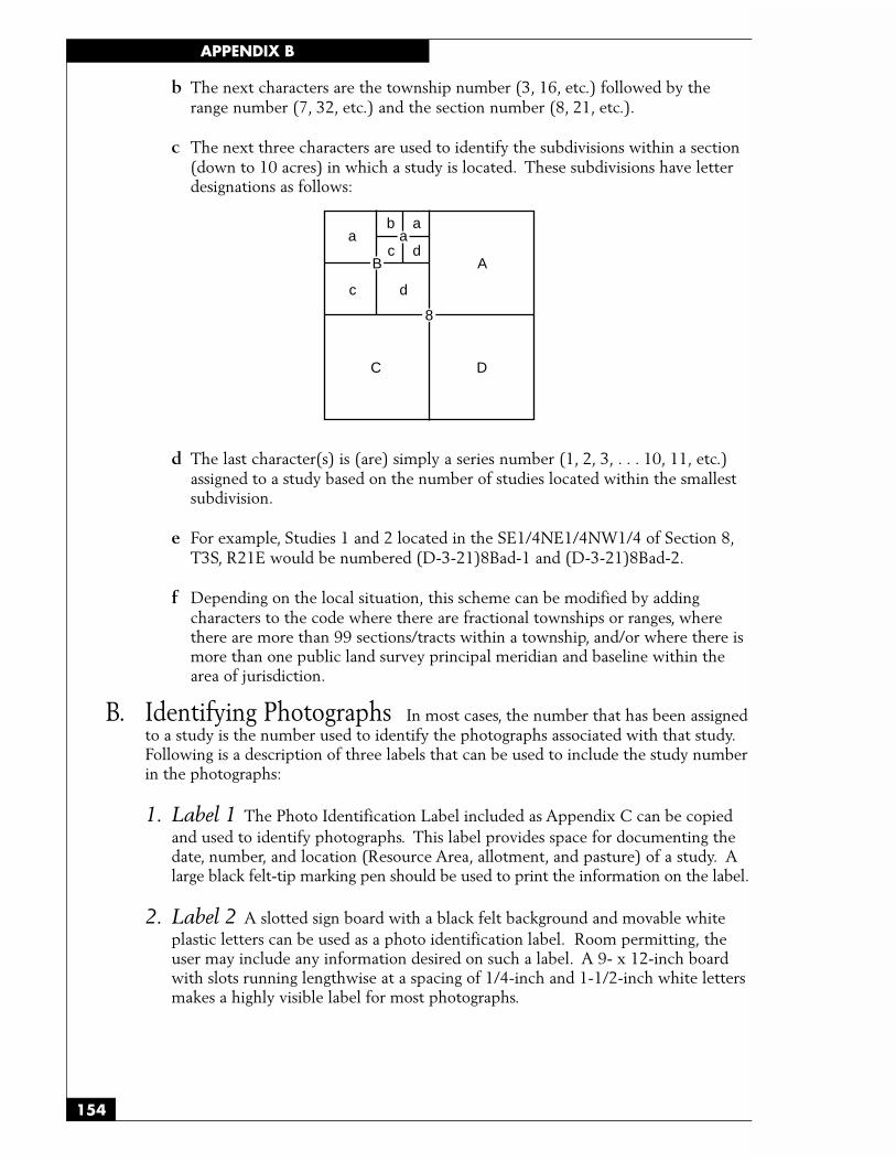
APPENDIX B
154
b The next characters are the township number (3, 16, etc.) followed by therange number (7, 32, etc.) and the section number (8, 21, etc.).
c The next three characters are used to identify the subdivisions within a section(down to 10 acres) in which a study is located. These subdivisions have letterdesignations as follows:
d The last character(s) is (are) simply a series number (1, 2, 3, . . . 10, 11, etc.)assigned to a study based on the number of studies located within the smallestsubdivision.
e For example, Studies 1 and 2 located in the SE1/4NE1/4NW1/4 of Section 8,T3S, R21E would be numbered (D-3-21)8Bad-1 and (D-3-21)8Bad-2.
f Depending on the local situation, this scheme can be modified by addingcharacters to the code where there are fractional townships or ranges, wherethere are more than 99 sections/tracts within a township, and/or where there ismore than one public land survey principal meridian and baseline within thearea of jurisdiction.
B. Identifying Photographs In most cases, the number that has been assignedto a study is the number used to identify the photographs associated with that study.Following is a description of three labels that can be used to include the study numberin the photographs:
1. Label 1 The Photo Identification Label included as Appendix C can be copiedand used to identify photographs. This label provides space for documenting thedate, number, and location (Resource Area, allotment, and pasture) of a study. Alarge black felt-tip marking pen should be used to print the information on the label.
2. Label 2 A slotted sign board with a black felt background and movable whiteplastic letters can be used as a photo identification label. Room permitting, theuser may include any information desired on such a label. A 9- x 12-inch boardwith slots running lengthwise at a spacing of 1/4-inch and 1-1/2-inch white lettersmakes a highly visible label for most photographs.
C D
A
a
d
b
ca
dc
a
B
8

155
APPENDIX B
3. Label 3 A placard on which identifying characteristics can be entered can bedeveloped to meet local field needs. The placard can be constructed of heavywhite cardboard on which such things as Date, “T” (township), “R” (range), Sec-tion Number, etc., are preprinted. A heavy mylar film can be placed over thepreprinted placard. The specific identifying information can be handprinted onthe mylar with a heavy grease pencil or other readily removable, highly visible,marking material. After taking the desired photographs, the mylar can be wipedclean and the placard reused for other photographs. A more permanent placardcan be constructed of plywood and painted enamel white. The grease pencilmarkings can be wiped from the enameled surface and the placard reused for otherphotographs. Caution must be exercised in the placement of the placard toprevent glare from the mylar or enameled surface.
NOTE - Labels can be placed flat on the ground immediately adjacent to photo plots forclose-up photographs.
- Labels can be placed in an upright position in the foreground of general viewphotographs.

APPENDIX B
156

157
APPENDIX C
APPENDIX C
Photo Identification Label
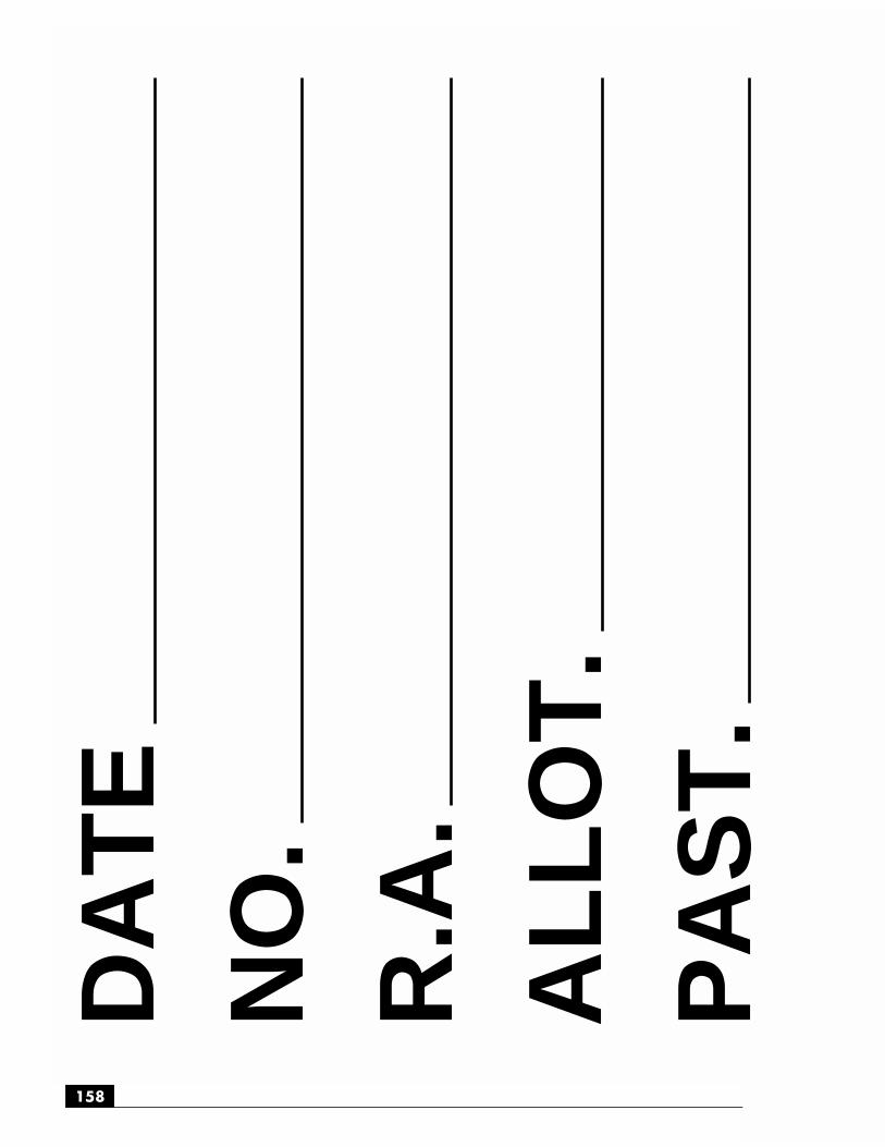
APPENDIX C
158
DA
TE
NO
.R
.A.
AL
LO
T.
PA
ST
.

APPENDIX C
160
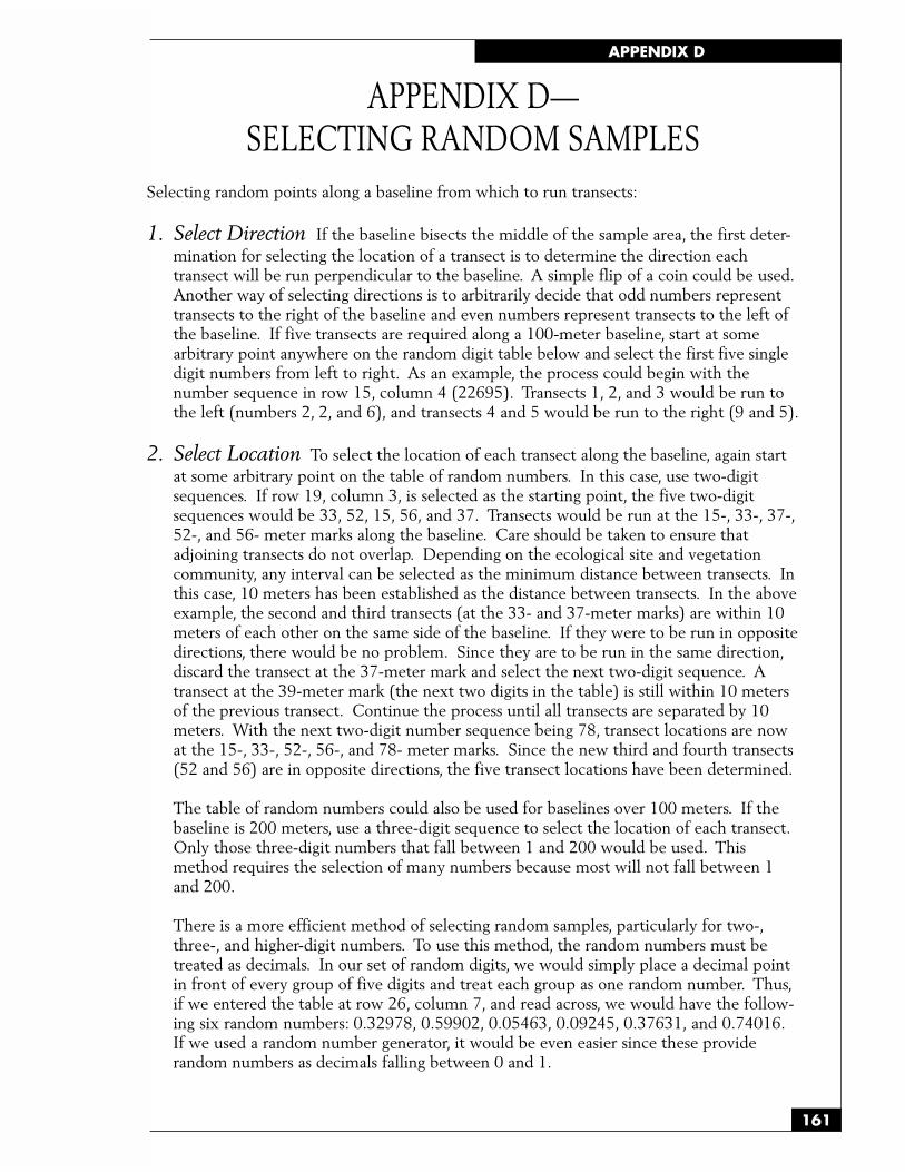
161
APPENDIX D
APPENDIX D—SELECTING RANDOM SAMPLES
Selecting random points along a baseline from which to run transects:
1. Select Direction If the baseline bisects the middle of the sample area, the first deter-mination for selecting the location of a transect is to determine the direction eachtransect will be run perpendicular to the baseline. A simple flip of a coin could be used.Another way of selecting directions is to arbitrarily decide that odd numbers representtransects to the right of the baseline and even numbers represent transects to the left ofthe baseline. If five transects are required along a 100-meter baseline, start at somearbitrary point anywhere on the random digit table below and select the first five singledigit numbers from left to right. As an example, the process could begin with thenumber sequence in row 15, column 4 (22695). Transects 1, 2, and 3 would be run tothe left (numbers 2, 2, and 6), and transects 4 and 5 would be run to the right (9 and 5).
2. Select Location To select the location of each transect along the baseline, again startat some arbitrary point on the table of random numbers. In this case, use two-digitsequences. If row 19, column 3, is selected as the starting point, the five two-digitsequences would be 33, 52, 15, 56, and 37. Transects would be run at the 15-, 33-, 37-,52-, and 56- meter marks along the baseline. Care should be taken to ensure thatadjoining transects do not overlap. Depending on the ecological site and vegetationcommunity, any interval can be selected as the minimum distance between transects. Inthis case, 10 meters has been established as the distance between transects. In the aboveexample, the second and third transects (at the 33- and 37-meter marks) are within 10meters of each other on the same side of the baseline. If they were to be run in oppositedirections, there would be no problem. Since they are to be run in the same direction,discard the transect at the 37-meter mark and select the next two-digit sequence. Atransect at the 39-meter mark (the next two digits in the table) is still within 10 metersof the previous transect. Continue the process until all transects are separated by 10meters. With the next two-digit number sequence being 78, transect locations are nowat the 15-, 33-, 52-, 56-, and 78- meter marks. Since the new third and fourth transects(52 and 56) are in opposite directions, the five transect locations have been determined.
The table of random numbers could also be used for baselines over 100 meters. If thebaseline is 200 meters, use a three-digit sequence to select the location of each transect.Only those three-digit numbers that fall between 1 and 200 would be used. Thismethod requires the selection of many numbers because most will not fall between 1and 200.
There is a more efficient method of selecting random samples, particularly for two-,three-, and higher-digit numbers. To use this method, the random numbers must betreated as decimals. In our set of random digits, we would simply place a decimal pointin front of every group of five digits and treat each group as one random number. Thus,if we entered the table at row 26, column 7, and read across, we would have the follow-ing six random numbers: 0.32978, 0.59902, 0.05463, 0.09245, 0.37631, and 0.74016.If we used a random number generator, it would be even easier since these providerandom numbers as decimals falling between 0 and 1.
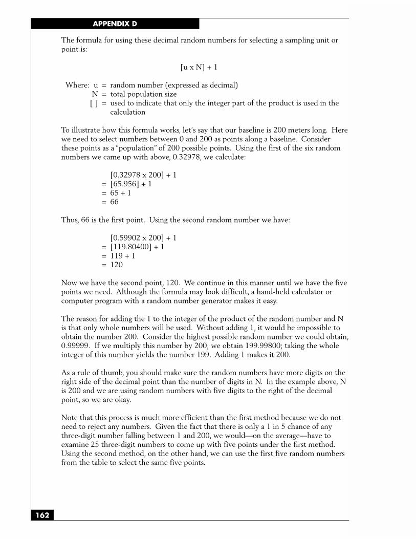
APPENDIX D
162
The formula for using these decimal random numbers for selecting a sampling unit orpoint is:
[u x N] + 1
Where: u = random number (expressed as decimal)N = total population size
[ ] = used to indicate that only the integer part of the product is used in thecalculation
To illustrate how this formula works, let’s say that our baseline is 200 meters long. Herewe need to select numbers between 0 and 200 as points along a baseline. Considerthese points as a “population” of 200 possible points. Using the first of the six randomnumbers we came up with above, 0.32978, we calculate:
[0.32978 x 200] + 1= [65.956] + 1= 65 + 1= 66
Thus, 66 is the first point. Using the second random number we have:
[0.59902 x 200] + 1= [119.80400] + 1= 119 + 1= 120
Now we have the second point, 120. We continue in this manner until we have the fivepoints we need. Although the formula may look difficult, a hand-held calculator orcomputer program with a random number generator makes it easy.
The reason for adding the 1 to the integer of the product of the random number and Nis that only whole numbers will be used. Without adding 1, it would be impossible toobtain the number 200. Consider the highest possible random number we could obtain,0.99999. If we multiply this number by 200, we obtain 199.99800; taking the wholeinteger of this number yields the number 199. Adding 1 makes it 200.
As a rule of thumb, you should make sure the random numbers have more digits on theright side of the decimal point than the number of digits in N. In the example above, Nis 200 and we are using random numbers with five digits to the right of the decimalpoint, so we are okay.
Note that this process is much more efficient than the first method because we do notneed to reject any numbers. Given the fact that there is only a 1 in 5 chance of anythree-digit number falling between 1 and 200, we would—on the average—have toexamine 25 three-digit numbers to come up with five points under the first method.Using the second method, on the other hand, we can use the first five random numbersfrom the table to select the same five points.
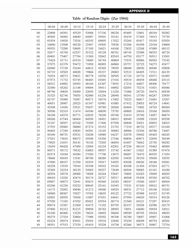
163
APPENDIX D
Table of Random Digits (Zar 1984)
00-04 05-09 10-14 15-19 20-24 25-29 30-34 35-39 40-44 45-49
00 22808 04391 45529 53968 57136 98228 85485 13801 68194 5638201 49305 36965 44849 64987 59501 35141 50159 57369 76913 7573902 81934 19920 73316 69243 69605 17022 53264 83417 55193 9292903 10840 13508 48120 22467 54505 70536 91206 81038 22418 3480004 99555 73289 59605 37105 24621 44100 72832 12268 97089 6811205 32677 45709 62337 35132 45128 96761 08745 53388 98353 4672406 09401 75407 27704 11569 52842 83543 44750 03177 50511 1530107 73424 31711 65519 74069 56744 40864 75315 89066 96563 7514208 37075 81378 59472 71858 86903 66860 03757 32723 54273 4547709 02060 37158 55244 44812 45369 78939 08048 28036 40946 0389810 94719 43565 40028 79866 43137 28063 52513 66405 71511 6613511 70234 48272 59621 88778 16536 36505 41724 24776 63971 0168512 07972 71752 92745 86465 01845 27416 50519 48458 68460 6311313 58521 64882 26993 48104 61307 73933 17214 44827 88306 7817714 32580 45202 21148 09684 39411 04892 02055 75276 51831 8568615 88796 30829 35009 22695 23694 11220 71006 26720 39476 6053816 31525 82746 78935 82980 61236 28940 96341 13790 66247 3383917 02747 35989 70387 89571 34570 17002 79223 96817 31681 1520718 46651 28987 20525 61347 63981 41085 67412 29053 00724 1484119 43598 14436 33521 55637 39789 26560 66404 71802 18763 8056020 30596 92319 11474 64546 60030 73795 60809 24016 29166 3605921 56198 64370 85771 62633 78240 05766 32419 35769 14057 8067422 68266 67544 06464 84956 18431 04015 89049 15098 12018 8933823 31107 28597 65102 75599 17496 87590 68848 33021 69855 5401524 37555 05069 38680 87274 55152 21792 77219 48732 03377 0116025 90463 27249 43845 94391 12145 36882 48906 52336 00780 7440726 99189 88731 93531 52638 54989 04237 32978 59902 05463 0924527 37631 74016 89072 59598 55356 27346 80856 80875 52850 3654828 73829 21651 50141 76142 72303 06694 61697 76662 23745 9628229 15634 89428 47090 12094 42134 62301 87236 90110 53463 4696930 00571 45172 78532 63863 98597 15742 41967 11821 91389 0747631 83374 10184 56384 27050 77700 13875 96607 76479 80535 1745432 78666 85645 13181 08700 08289 62956 54439 39150 95690 1855533 47890 88197 21358 65254 35917 54035 83028 84636 38186 5058134 56238 13559 79344 83198 94542 35165 40188 21456 67024 6277135 35369 32234 38129 59963 99237 72648 66504 99065 61161 1618636 42934 34578 28968 74028 42164 55647 76805 61023 33099 4829337 09010 15226 43474 30174 26727 39317 48508 55438 85336 4076238 83897 90073 72941 85613 85569 24183 08247 15946 02957 6850439 82206 01230 93252 89045 25141 91943 75531 87420 99012 8075140 14175 32992 49046 41272 94040 44929 98531 27712 05106 3524241 58968 88367 70927 74765 18635 85122 27722 95388 61523 9174542 62601 04595 76926 11007 67631 64641 07994 04639 39314 8312643 97030 71165 47032 85021 65554 66774 21560 04121 57297 8541544 89074 31587 21360 41673 71192 85795 82157 52928 62586 0217945 07806 81312 81215 99858 26762 28993 74951 64680 50934 3201146 91540 86466 13229 76624 44092 96604 08590 89705 03424 4803347 99279 27334 33804 77988 93592 90708 56780 70097 39907 5100648 63224 05074 83941 25034 43516 22840 35230 66048 80754 4630249 98351 97513 27529 65419 35328 19738 82366 38573 50967 72754

Form ApprovedOMB No. 0704-0188
Public reporting burden for this collection of information is estimated to average 1 hour per response, including the time for reviewing instructions, searching existing data sources, gathering andmaintaining the data needed, and completing and reviewing the collection of information. Send comments regarding this burden estimate or any other aspect of this collection of information,including suggestions for reducing this burden, to Washington Headquarters Services, Directorate for Information Operations and Reports, 1215 Jefferson Davis Highway, Suite 1204, Arlington,VA 22202-4302, and to the Office of Management and Budget, Paperwork Reduction Project (0704-0188), Washington, DC 20503.
5. FUNDING NUMBERS
12b. DISTRIBUTION CODE
18. SECURITY CLASSIFICATIONOF THIS PAGE
20. LIMITATION OF ABSTRACT
Standard Form 298 (Rev. 2-89)Prescribed by ANSI Std. Z39-18
298-102
NSN 7540-01-280-5500
REPORT DOCUMENTATION PAGE
4. TITLE AND SUBTITLE
1. AGENCY USE ONLY (Leave blank) 2. REPORT DATE 3. REPORT TYPE AND DATES COVERED
6. AUTHOR(S)
7. PERFORMING ORGANIZATION NAME(S) AND ADDRESS(ES) 8. PERFORMING ORGANIZATIONREPORT NUMBER
9. SPONSORING/MONITORING AGENCY NAME(S) AND ADDRESS(ES) 10. SPONSORING/MONITORINGAGENCY REPORT NUMBER
11. SUPPLEMENTARY NOTES
12a. DISTRIBUTION/AVAILABILITY STATEMENT
13. ABSTRACT (Maximum 200 words)
14. SUBJECT TERMS 15. NUMBER OF PAGES
16. PRICE CODE
17. SECURITY CLASSIFICATIONOF REPORT
19. SECURITY CLASSIFICATIONOF ABSTRACT
Sampling Vegetation Attributes
Interagency Technical Team
U.S. Department of the InteriorBureau of Land Management - National Applied Resource Sciences CenterP.O. Box 25047Denver, CO 80225-0047
BLM/RS/ST-96/002+1730
• Rangeland inventory • Vegetation attributes• Rangeland monitoring • Vegetation sampling• Rangeland evaluation
Unclassified Unclassified
June 1996 Final
Unclassified UL
This interagency technical reference provides the basis for consistent, uniform, andstandard vegetation attribute sampling that is economical, repeatable, statisticallyreliable, and technically adequate. While not all inclusive, this reference does includethe primary vegetation sampling methods used across the West (frequency methods, dryweight rank method, Daubenmire, line intercept, density method, comparative yield,etc.).
176, including covers


