The Effect of Population Density on Housing Prices: A Cross State Analysis Senior Thesis Department of Economics May 2016 By: Andrew Souders Advisors: Dr. Francesco Renna & Dr. Amanda Weinstein
Transcript
The Effect of Population Density on Housing Prices: A Cross State Analysis
Senior Thesis
Department of Economics
May 2016
By: Andrew Souders
Advisors: Dr. Francesco Renna & Dr. Amanda Weinstein
1
Abstract:
This paper examines how various factors affect the price we pay for a house. I examine if
what are considered to be amenities do indeed have a positive effect on the value of the house
and disamenities have a negative effect on the value of the house. My study covers various states
across the United States, these states are then compared to one another to see the effect of the
bundle of amenities across these states, my main variable of interest is population density. I use a
quadratic hedonic pricing model on my data. I then compare the results across states to determine
if variables are valued the same on a state to state basis. I find the population density to have a
both a positive and negative impact on housing prices. This indicates that households view
population density differently depending on the state and the level of population density.
2
Table of Contents
I. Abstract………………………………………………………....…………………………1
II. Introduction…………………………………………………………………………….….3
II. Literature Review………………………………………………………………………....5
III. Theoretical Model……………………………………………………………....……...….9
IV. Econometric Model & Data……………………………………………………………...11
V. Results……………………………………………………………………………...…….14
VI. Conclusion………………………………………………………………………....…….18
VII. Appendix………….……………………………………………..……....…………...….21
VIII. References…………………………………………………………………….………….28
3
I. Introduction
Hedonic pricing is a useful tool because it can elicit how much value individuals place on
certain amenities. It is especially useful for pricing amenities for which it is hard to put an exact
price tag on. For example when you are asked if you would rather live in an area with more or
less pollution, you are going to answer the area with less pollution. If that question were
rephrased into how much are you willing to pay to live in an area with less pollution, it is hard to
put an exact dollar amount on the value of less pollution. The benefit of the hedonic method is
that it does not rely on survey respondents to answer questions, rather it is a revealed preference
method of assessing how people value an amenity. The revealed preference method is a method
where the preferences of individuals are shown through their purchasing history. In the case of
housing, the preferences are revealed through how much people pay for houses with certain
characteristics. Policymakers can use this pricing method if they want to determine how much
money to spend on reducing pollution by building a park for they can measure how much people
living in an area near the park will benefit due to the change in pollution levels. The policy
makers will then be able to calculate the net benefit to the residents based on prior research
which has shown the effects of pollution on housing prices.
In my research I will be examining the value of individual houses across states. My
research will provide a view of how households across states values population density as either
an amenity or disamenity. There is an ongoing debate between whether or not population density
is an amenity or disamenity. This debate stems from two pertinent arguments regarding the
nature of density. Those in favor of density argue that density is desirable because it brings
people together and knowledge will be shared among people. This sharing of knowledge is
4
formerly known as knowledge spillover. Agglomeration is also a product of density,
agglomeration is where firms and people are located near each other resulting in an economies of
scale effect. This economies of scale effect based on agglomeration is good because firms will
become more efficient and workers more productive.
The argument against density is based on the negative externalities of density. These
externalities include congestion, pollution and crime rates. Typically people value these factors
as economic bads. This means that people would expect to be compensated for having to
experience these resources, think of them as the opposite of an economic good which you have
to pay for.
Based on the highlights both for and against density, it appears that the actual effects of
density on housing prices depend on which factors dominate the other in the eyes of the
consumer. The effects of these variables are ambiguous, in my study I am going to attempt to
answer how consumers generally regard density through their revealed preferences.
My research will build off of prior hedonic pricing research that has been completed by
my forbearers. My research will add to the field by offering a cross state comparison, with a
focus on whether density is an amenity or disamenity and determine whether the housing market
is homogeneous. Research has been done that has concluded that the U.S. housing market is not
heterogeneous, conflicting research has been done that has determined that there are differences
between cities. Previously, research has collected data at the Metropolitan Statistical Area
(MSA) level or in certain neighborhoods of cities. Instead, I examine the relationship at the
Public Use Microdata Areas (PUMA) level. I am using population density and climatic data
gathered at the PUMA level. I am using the PUMA level because this includes rural areas and
not just urban areas. I believe that rural areas need to be included in my analysis because I want
5
to fully represent each state and the inclusion of both rural and urban areas will allow me to do
so. All household and individual data is gathered from the American Community Survey (ACS)
2013. Climatic data is gathered from PRISM Climate Group (1981-2010) 30 year Climate
Normals. Population density data was obtained from 2012 ESRI Demographic Data. Population
density is measured in, population/mi2.
II. Literature Review
Roback (1982) examined how much residents are willing to pay to for various amenities.
Roback found the density variable positively impacted land prices with an increase in population
density by 100 people/square leading to an increase in land price of $6.30. Roback used SMSAs
(Standard Metropolitan Statistical Areas) for her unit of measure in calculating density.
Blomquist et al. (1988) used individual housing data instead of using groups of housing,
which is what Roback previously did. Blomquist et al. ran two different regressions, the first
regression included only physical housing attributes. The second regression included a variety of
amenities ranging from weather related amenities such as precipitation and sunshine to other
community related variables, such as violent crime rates and teacher-pupil ratio. To model for
density in their study they used a proxy for density which was a dummy variable for whether or
not the resident lived in the central city. They found that a person who lived in a central city
location would pay $40.75 per year to do so. This indicates that central city location is an
amenity in this paper because people are willing to pay to be there rather than being subsidized
for living in the central city location.
Sirmans et al. (2006), run a meta regression analysis of the nine most used housing
characteristics in hedonic house price regressors, which are square footage, lot size, age,
bedrooms, bathrooms, garage, swimming pool, fireplace, and air conditioning. What they are
6
looking for specifically is how the coefficients vary in terms of geographical location, time, data
source, median income, the number of regressors in the hedonic price equation, and the use of
control variables. What they found was that most variation between the coefficients was due to
the geographical location of the house especially for the characteristics of square footage, lot
size, age, bathrooms, swimming pool, and air conditioning. This paper shows that different
hedonic estimates do experience some significant variation, but not as much as is traditionally
believed. This is important because it means that to some extent most hedonic methods for
calculating housing prices although different in many cases have generally the same results,
which is important for the sake of consistency and reliability of the hedonic method.
Linneman (1978) reviews the standard estimation procedures for fitting hedonic functions
along with the evaluation in the difference in the national housing market among cities. In this
paper he compares Los Angeles and Chicago with the national average in an attempt to see if the
housing market is homogeneous. A homogeneous housing market is one in which people value
amenities the same across the whole market and preferences are not assumed to vary. He notes
the potential biases that face the hedonic pricing method. These biases include functional form
owner-renter selection sample bias as well as the omitted variable bias. He confronts those
various biases in his paper through his research of comparing Chicago and Los Angeles with one
another and national averages in housing prices and amenity variables. In his analysis he
considers both physical household characteristics along with a variety of neighborhood traits
such as if the neighborhood is considered bad or if the school quality is considered bad. He uses
Chicago because he defined it as an older city and Los Angeles as a newer city to see if there is a
difference between the two areas and how they compared to the national average.
7
Linneman runs a hedonic pricing method which comprised of two parts. First was the
housing structural vector, which comprised of the physical characteristics of the house. The
second part was the non-structural vector, which comprises of neighborhood amenities not
directly related to the house. These vectors comprised of an agglomeration of the different
physical housing characteristics along with an agglomeration of the various neighborhood traits.
In his analysis he attempts to see if the two areas differed from the national average in pricing of
amenities, but he found that with 95% confidence that he could not reject the null hypothesis
which was, the functional specification (difference in cities) was the same as the national model.
This supports the claim that the nation as a whole is a homogeneous housing market, which
means that preferences are generally the same across cities. For example somebody in New York
values sunlight as much as somebody in Oregon. However, Dunse et al. (2013) argue against this
conclusion.
Dunse et al. (2013) examine the effect of density on housing prices in five different cities
throughout England. They decide on the five cities based on the variation in terms of housing
density, geographic location economic prosperity of the city and the size of the metropolitan
area. Dunse et al. (2013) then construct a hedonic pricing model to include attributes that
represented the physical aspects of the housing units, the location, neighborhood externalities,
and dwelling type, mix and density. They decide to test their main variable of density in the
hedonic model non-linearly. They hadn’t found any suggestions in economic theory that the
relationship between housing prices and density should be either linear or nonlinear. Dunse et al.
(2013) decide that the nonlinear quadratic relationship between housing prices and density fit
their data best. I will be testing a nonlinear method in my paper as well. In their estimation, they
8
model density through the actual dwelling density which is defined as: The dwelling density for
the census output area of each house in their data.
What they find in their results is that dwelling density is statistically significant across all
areas. Density is found to have differing effects on the price of the house depending on where it
is located. For example the relationship between dwellings per hectare is convex in some areas.
Meaning that at a certain point as housing prices decrease with increasing density a point of
inflection is reached and the housing prices then increase with increases in density. This
relationship is similar to that of a u-shape. In London the opposite is found to be true. The
relationship between housing prices and density is concave. Meaning that as density increases
housing prices increase, until a point of inflection is reached where increases in density are met
with decreases in housing prices. This forms an upside down u-shape. These contrasting
relationships between density and housing prices highlight the ambiguity with the relationship
between these two factors. The paper concludes that each city must be taken into account
individually when implementing policy changes to the housing market.
This previous literature builds the base off of which my paper stands. My main focus will
be on the impact of density on the value of a house examining how households value population
density and whether there is a nonlinear relationship in how they value density. Density is a
factor that has been previously studied and many researchers disagree on the effects that density
has on the price of housing and whether to consider it an amenity or disamenity. The literature
also disagrees on whether the value of this amenity, along with others varies across space. I add
to the literature by addressing these disagreements I previously stated between the literature.
9
III. Theoretical Model
The idea of the hedonic housing price model is rooted in the theory of supply and
demand. The housing market is comprised of buyers and sellers. On one side, there is the
demand, the buyer, and on the other side, is the supply, the seller. A house is sold at the point
where the buyer and seller agree on a fair price to pay for the house. This housing value they
agree upon is based on the physical characteristics of the house along with other characteristics
of the surrounding environment such as the school district and crime rate. When buying a house
the buyer considers all of these factors when determining how much to offer for the house. The
seller is also going through this calculation and deciding what price to sell the house for, trying
to get a sense for what the demand will be for his house. The agreed upon price would indicate
how much the buyer values the environment the house is located in as well as the actual physical
components of the house.
The hedonic pricing model attempts to quantify the exact amount that each characteristic
is worth based on the current value of a property. This is referred to as the revealed preferences
method of estimating value because the preferences for certain amenities are revealed through
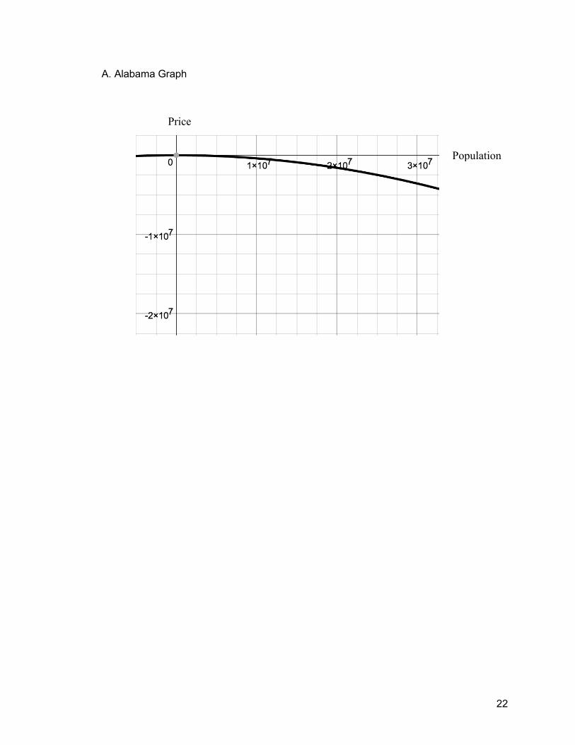
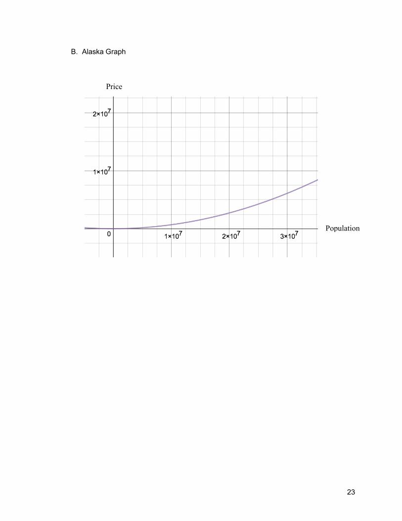
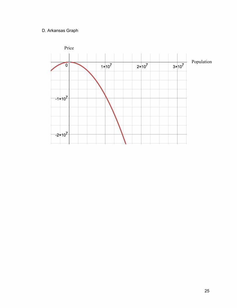
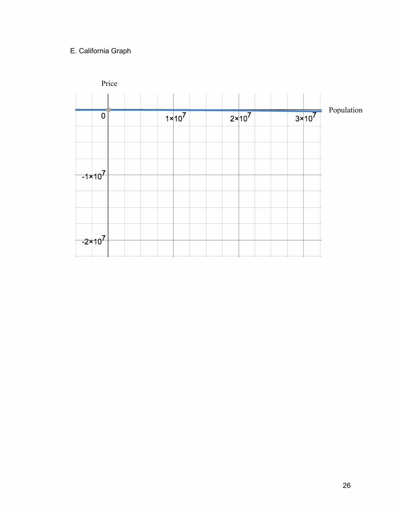
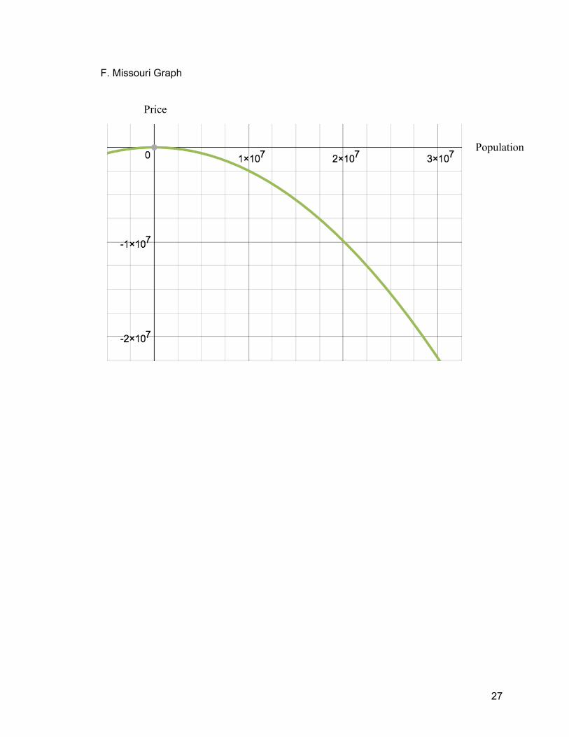
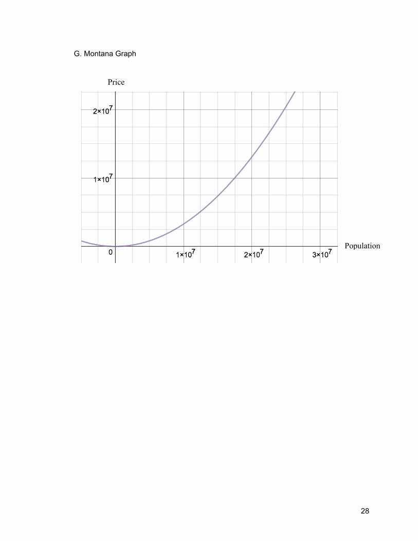
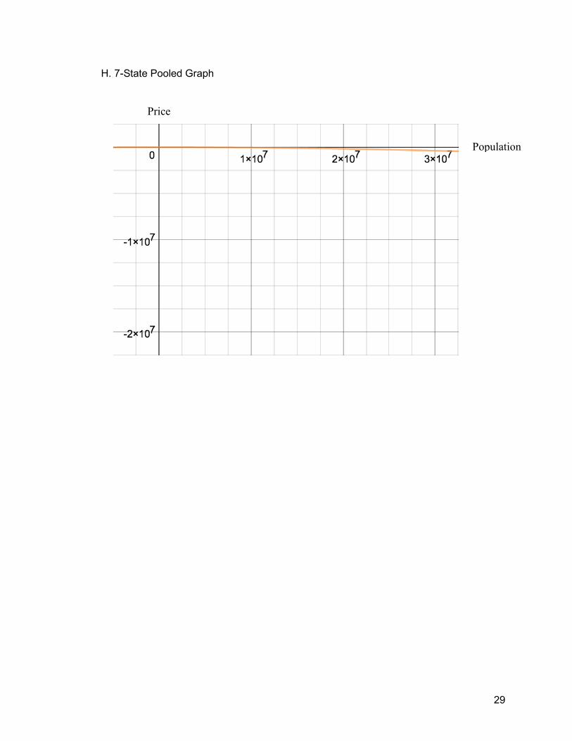
the agreed upon price. The below graphs illustrate the relationship between population density
and housing prices. If population density is an amenity then housing prices will increase with
increases in density, this is illustrated in Graph 1. If increases in population density result in
lower prices population density is considered a disamenity, this is illustrated in Graph 2.
10
Figure(1) Figure(2)
When purchasing a house individuals are attempting to maximize their own utility subject
to a budget constraint. This means that given a certain income individuals choose the optimal
combination of both housing and consumption of other goods and services. This relates to the
idea of individuals are willing to pay to live in better school district and low crime rates
neighborhood. To consume these amenities the individual must give up some housing to stay on
the same level of utility. Figure (1) below illustrates this concept. The concept of utility
maximization is important because it follows the idea that the housing value directly represents
the utility of living in a given housing unit in a given geographical region with certain
surrounding amenities.
Figure (3)
(Economics Help, 2012)
11
My study in particular will examine how residents value certain amenities. The revealed
value of these amenities will be compared between 7 states to see if there are differences in value
placed on certain amenities, with a specific focus on the density variable. I will determine the
value they place on these amenities based on how much they are paying for housing. I
hypothesize that an increase in the level of population density will result in a quadratic
relationship to housing prices and this relationship may differ or be constant from state to state.
This hypothesis is derived from the economic concept of housing being considered a normal
good, as well as density being shown to have both positive and negative effects on housing
prices. The conflicting literature between whether density should differ between areas makes it
hard for me to know which one will be right and I will proceed in attempt to see which way my
results follow.
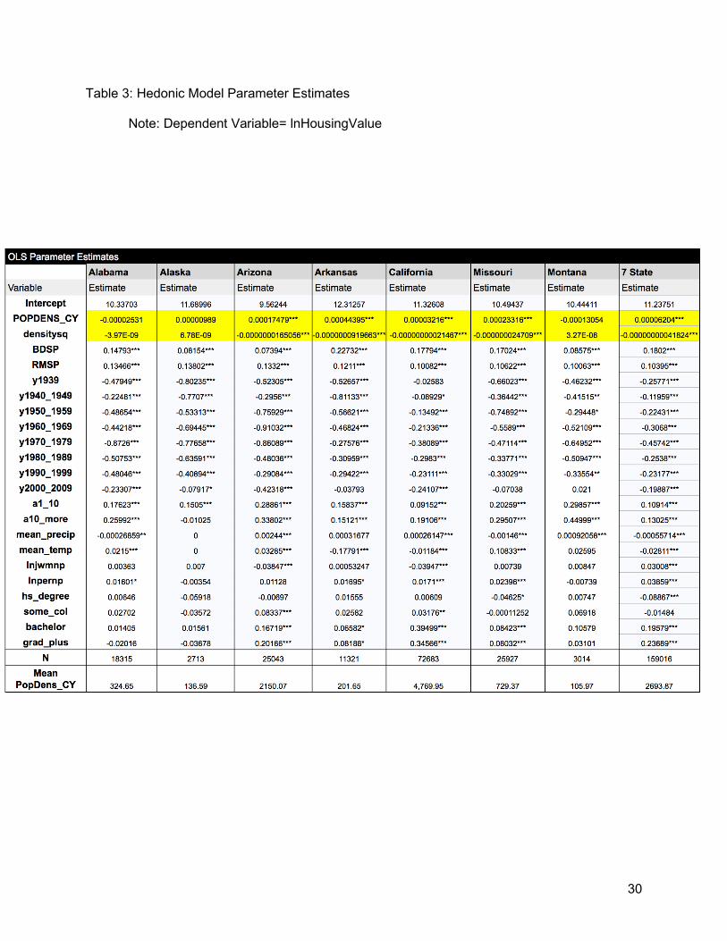
IV. Econometric Model & Data
I have decided to use the quadratic form to model population density. The use of this
model allows population density to increase and decrease depending on the amount of population
density. The quadratic modeling of density is important because it denotes how people value
density compared to housing prices and allows for the relationship to change. I have decided to
include a quadratic equation because based on Dunse et al. (2013) paper, they showed that
density may not always have a strictly linear relationship with housing prices.
Other amenities are necessary to give a complete estimate of the price of a house, I have
included variables to represent the physical component of the house, the community aspect of a
house and weather related variables. According to economic theory, housing prices should
increase as amenities increase. Amenities will have a positive effect on the household because
people naturally want more of them. As incomes increase people will want to consume both
12
more physical housing and other neighborhood amenities, such as a safer environment or an area
with more educated people.
Throughout this paper a pair of underlying assumptions must be noted. First of all
housing prices may not be the only factor that are affected by various amenities. For example
somebody may be willing to not only pay more to live in an area that is educated, they may be
willing to accept lower wages to live in that area. This would mean that by solely focusing on the
housing prices that the real effect of education on the value of an area is being underrepresented.
This means that my research will serve as a lower bound for how we value certain amenities.
Another concept that must be noted is that the housing market for the United States is
considered homogeneous as in Linneman (1978). This means that amenities and other variables
should have similar impacts throughout the United States since the market is considered
homogeneous. To put this in direct terms with my research, density according to Linneman is
valued equally by everyone across the 7 states I will be studying, from a person living in an
apartment complex in California, to a farmer living in Arkansas. This idea is contrary to Dunse et
al. (2013) paper. I will be expanding on this idea to see if the market truly is homogeneous, or if
preferences need to be taken on state by state basis as suggested by Dunse et al. (2013).
Where my research will differ from prior research is that I will be evaluating individual
households, but grouping characteristics such as precipitation, temperature and density which are
normally gathered at the county level to the smaller defined PUMA level. I will then categorize
my data based on the corresponding state of the data observation. My research will also offer a
comparison of amenities across states, while at the same time determining if density is valued the
same across states.
13
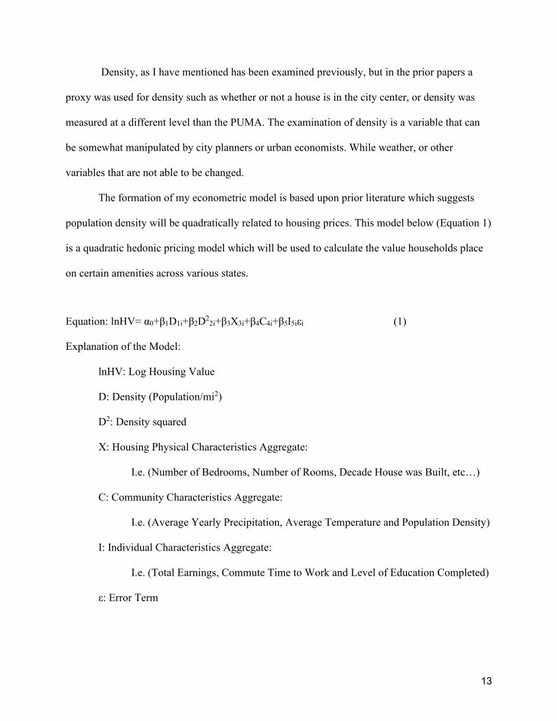
Density, as I have mentioned has been examined previously, but in the prior papers a
proxy was used for density such as whether or not a house is in the city center, or density was
measured at a different level than the PUMA. The examination of density is a variable that can
be somewhat manipulated by city planners or urban economists. While weather, or other
variables that are not able to be changed.
The formation of my econometric model is based upon prior literature which suggests
population density will be quadratically related to housing prices. This model below (Equation 1)
is a quadratic hedonic pricing model which will be used to calculate the value households place