307
Sergiu Vacaru and Panayiotis Stavrinos SPINORS and SPACE–TIME ANISOTROPY University of Athens ————————————————— c Sergiu Vacaru and Panyiotis Stavrinos

Sergiu Vacaru and Panayiotis Stavrinos
SPINORSand
SPACE–TIME ANISOTROPY
University of Athens
—————————————————c© Sergiu Vacaru and Panyiotis Stavrinos

ii
-

i
ABOUT THE BOOK
This is the first monograph on the geometry of anisotropic spinor spaces andits applications in modern physics. The main subjects are the theory of grav-ity and matter fields in spaces provided with off–diagonal metrics and asso-ciated anholonomic frames and nonlinear connection structures, the algebraand geometry of distinguished anisotropic Clifford and spinor spaces, theirextension to spaces of higher order anisotropy and the geometry of gravityand gauge theories with anisotropic spinor variables. The book summarizesthe authors’ results and can be also considered as a pedagogical survey onthe mentioned subjects.

ii
-

iii
ABOUT THE AUTHORS
Sergiu Ion Vacaru was born in 1958 in the Republic of Moldova. He waseducated at the Universities of the former URSS (in Tomsk, Moscow, Dubnaand Kiev) and reveived his PhD in theoretical physics in 1994 at ”Al. I. Cuza”University, Iasi, Romania. He was employed as principal senior researcher, as-sociate and full professor and obtained a number of NATO/UNESCO grantsand fellowships at various academic institutions in R. Moldova, Romania,Germany, United Kingdom, Italy, Portugal and USA. He has published inEnglish two scientific monographs, a university text–book and more thanhundred scientific works (in English, Russian and Romanian) on (super)gravity and string theories, extra–dimension and brane gravity, black holephysics and cosmolgy, exact solutions of Einstein equations, spinors andtwistors, anistoropic stochastic and kinetic processes and thermodynamicsin curved spaces, generalized Finsler (super) geometry and gauge gravity,quantum field and geometric methods in condensed matter physics.
Panayiotis Stavrinos is Assistant Professor in the University of Athens,where he obtained his Ph. D in 1990 and hold lecturer positions during1990-1999. He is a Founding Member and Vice President of Balkan Soci-ety of Geometers , Member of the Editorial Board of the Journal of BalkanSociety. Honorary Member to The Research Board of Advisors, AmericanBiographical Institute (U.S.A.), 1996. Member of Tensor Society, (Japan),1981. Dr. Stavrinos has published over 40 research works in different in-ternational Journals in the topics of local differential geometry, Finsler andLagrange Geometry, applications of Finsler and Lagrange geometry to grav-itation, gauge and spinor theory as well as Einstein equations, deviation ofgeodesics, tidal forces, weak gravitational fields, gravitational waves. He isco-author in the monograph ”Introduction to the Physical Principles of Dif-ferential Geometry”, in Russian, published in St. Petersburg in 1996 (secondedition in English, University of Athens Press, 2000). He has publishedtwo monographs in Greek for undergraduate and graduate students in theDepartment of Mathematics and Physics : ”Differential Geometry and itsApplications Vol. I, II (University of Athens Press, 2000).

iv

Contents
0.1 Preface . . . . . . . . . . . . . . . . . . . . . . . . . . . . . . . vii0.1.1 Historical remarks on spinor theory . . . . . . . . . . . vii0.1.2 Metric Spaces depending on Spinor Variables and Gauge
Field Theories . . . . . . . . . . . . . . . . . . . . . . . ix0.1.3 Nonlinear connection geometry and physics . . . . . . . x0.1.4 Anholonomic frames and nonlinear connections in Ein-
stein gravity . . . . . . . . . . . . . . . . . . . . . . . . xiv0.1.5 The layout of the book . . . . . . . . . . . . . . . . . . xvi0.1.6 Acknowledgments . . . . . . . . . . . . . . . . . . . . xvii
0.2 Notation . . . . . . . . . . . . . . . . . . . . . . . . . . . . . . xix
I Space–Time Anisotropy 1
1 Vector Bundles and N–Connections 31.1 Vector and Covector Bundles . . . . . . . . . . . . . . . . . . 4
1.1.1 Vector and tangent bundles . . . . . . . . . . . . . . . 41.1.2 Covector and cotangent bundles . . . . . . . . . . . . . 51.1.3 Higher order vector/covector bundles . . . . . . . . . . 6
1.2 Nonlinear Connections . . . . . . . . . . . . . . . . . . . . . . 101.2.1 N–connections in vector bundles . . . . . . . . . . . . . 101.2.2 N–connections in covector bundles: . . . . . . . . . . . 111.2.3 N–connections in higher order bundles . . . . . . . . . 121.2.4 Anholonomic frames and N–connections . . . . . . . . 13
1.3 Distinguished connections and metrics . . . . . . . . . . . . . 191.3.1 D–connections . . . . . . . . . . . . . . . . . . . . . . . 191.3.2 Metric structure . . . . . . . . . . . . . . . . . . . . . . 221.3.3 Some remarkable d–connections . . . . . . . . . . . . . 251.3.4 Amost Hermitian anisotropic spaces . . . . . . . . . . . 27
1.4 Torsions and Curvatures . . . . . . . . . . . . . . . . . . . . . 291.4.1 N–connection curvature . . . . . . . . . . . . . . . . . 291.4.2 d–Torsions in v- and cv–bundles . . . . . . . . . . . . . 30
v

vi CONTENTS
1.4.3 d–Curvatures in v- and cv–bundles . . . . . . . . . . . 31
1.5 Generalizations of Finsler Spaces . . . . . . . . . . . . . . . . 32
1.5.1 Finsler Spaces . . . . . . . . . . . . . . . . . . . . . . . 321.5.2 Lagrange and Generalized Lagrange Spaces . . . . . . . 34
1.5.3 Cartan Spaces . . . . . . . . . . . . . . . . . . . . . . . 35
1.5.4 Generalized Hamilton and Hamilton Spaces . . . . . . 37
1.6 Gravity on Vector Bundles . . . . . . . . . . . . . . . . . . . . 38
2 Anholonomic Einstein and Gauge Gravity 412.1 Introduction . . . . . . . . . . . . . . . . . . . . . . . . . . . . 41
2.2 Anholonomic Frames . . . . . . . . . . . . . . . . . . . . . . . 42
2.3 Higher Order Anisotropic Structures . . . . . . . . . . . . . . 48
2.3.1 Ha–frames and corresponding N–connections . . . . . . 482.3.2 Distinguished linear connections . . . . . . . . . . . . . 52
2.3.3 Ha–torsions and ha–curvatures . . . . . . . . . . . . . 54
2.3.4 Einstein equations with respect to ha–frames . . . . . . 552.4 Gauge Fields on Ha–Spaces . . . . . . . . . . . . . . . . . . . 56
2.4.1 Bundles on ha–spaces . . . . . . . . . . . . . . . . . . . 57
2.4.2 Yang-Mills equations on ha-spaces . . . . . . . . . . . . 60
2.5 Gauge Ha-gravity . . . . . . . . . . . . . . . . . . . . . . . . . 632.5.1 Bundles of linear ha–frames . . . . . . . . . . . . . . . 64
2.5.2 Bundles of affine ha–frames and Einstein equations . . 65
2.6 Nonlinear De Sitter Gauge Ha–Gravity . . . . . . . . . . . . . 662.6.1 Nonlinear gauge theories of de Sitter group . . . . . . . 67
2.6.2 Dynamics of the nonlinear de Sitter ha–gravity . . . . 69
2.7 An Ansatz for 4D d–Metrics . . . . . . . . . . . . . . . . . . . 72
2.7.1 The h–equations . . . . . . . . . . . . . . . . . . . . . 742.7.2 The v–equations . . . . . . . . . . . . . . . . . . . . . 75
2.7.3 H–v equations . . . . . . . . . . . . . . . . . . . . . . . 76
2.8 Anisotropic Cosmological Solutions . . . . . . . . . . . . . . . 772.8.1 Rotation ellipsoid FRW universes . . . . . . . . . . . . 77
2.8.2 Toroidal FRW universes . . . . . . . . . . . . . . . . . 79
2.9 Concluding Remarks . . . . . . . . . . . . . . . . . . . . . . . 80
3 Anisotropic Taub NUT – Dirac Spaces 85
3.1 N–connections in General Relativity . . . . . . . . . . . . . . . 853.1.1 Anholonomic Einstein–Dirac Equations . . . . . . . . . 88
3.1.2 Anisotropic Taub NUT – Dirac Spinor Solutions . . . . 94
3.2 Anisotropic Taub NUT Solutions . . . . . . . . . . . . . . . . 96
3.2.1 A conformal transform of the Taub NUT metric . . . . 97

CONTENTS vii
3.2.2 Anisotropic Taub NUT solutions with magnetic polar-ization . . . . . . . . . . . . . . . . . . . . . . . . . . . 99
3.3 Anisotropic Taub NUT–Dirac Fields . . . . . . . . . . . . . . 1013.3.1 Dirac fields and angular polarizations . . . . . . . . . . 1013.3.2 Dirac fields and extra dimension polarizations . . . . . 103
3.4 Anholonomic Dirac–Taub NUT Solitons . . . . . . . . . . . . 1043.4.1 Kadomtsev–Petviashvili type solitons . . . . . . . . . . 1053.4.2 (2+1) sine–Gordon type solitons . . . . . . . . . . . . . 106
II Anisotropic Spinors 109
4 Anisotropic Clifford Structures 1134.1 Distinguished Clifford Algebras . . . . . . . . . . . . . . . . . 1134.2 Anisotropic Clifford Bundles . . . . . . . . . . . . . . . . . . . 118
4.2.1 Clifford d-module structure . . . . . . . . . . . . . . . 1184.2.2 Anisotropic Clifford fibration . . . . . . . . . . . . . . 120
4.3 Almost Complex Spinors . . . . . . . . . . . . . . . . . . . . . 121
5 Spinors and Anisotropic Spaces 1275.1 Anisotropic Spinors and Twistors . . . . . . . . . . . . . . . . 1285.2 Mutual Transforms of Tensors and Spinors . . . . . . . . . . . 133
5.2.1 Transformation of d-tensors into d-spinors . . . . . . . 1335.2.2 Fundamental d–spinors . . . . . . . . . . . . . . . . . 134
5.3 Anisotropic Spinor Differential Geometry . . . . . . . . . . . . 1355.4 D-covariant derivation . . . . . . . . . . . . . . . . . . . . . . 1365.5 Infeld - van der Waerden coefficients . . . . . . . . . . . . . . 1385.6 D-spinors of Anisotropic Curvature and Torsion . . . . . . . . 140
6 Anisotropic Spinors and Field Equations 1436.1 Anisotropic Scalar Field Interactions . . . . . . . . . . . . . . 1436.2 Anisotropic Proca equations . . . . . . . . . . . . . . . . . . . 1456.3 Anisotropic Gravitons and Backgrounds . . . . . . . . . . . . 1466.4 Anisotropic Dirac Equations . . . . . . . . . . . . . . . . . . 1466.5 Yang-Mills Equations in Anisotropic Spinor Form . . . . . . . 147
III Higher Order Anisotropic Spinors 149
7 Clifford Ha–Structures 1537.1 Distinguished Clifford Algebras . . . . . . . . . . . . . . . . . 1537.2 Clifford Ha–Bundles . . . . . . . . . . . . . . . . . . . . . . . 158

viii CONTENTS
7.2.1 Clifford d–module structure in dv–bundles . . . . . . . 158
7.2.2 Clifford fibration . . . . . . . . . . . . . . . . . . . . . 160
7.3 Almost Complex Spinor Structures . . . . . . . . . . . . . . . 161
8 Spinors and Ha–Spaces 165
8.1 D–Spinor Techniques . . . . . . . . . . . . . . . . . . . . . . . 165
8.1.1 Clifford d–algebra, d–spinors and d–twistors . . . . . . 166
8.1.2 Mutual transforms of d-tensors and d-spinors . . . . . 169
8.1.3 Transformation of d-tensors into d-spinors . . . . . . . 169
8.1.4 Fundamental d–spinors . . . . . . . . . . . . . . . . . 170
8.2 Differential Geometry of Ha–Spinors . . . . . . . . . . . . . . 171
8.2.1 D-covariant derivation on ha–spaces . . . . . . . . . . 172
8.2.2 Infeld–van der Waerden coefficients . . . . . . . . . . . 174
8.2.3 D–spinors of ha–space curvature and torsion . . . . . . 176
9 Ha-Spinors and Field Interactions 179
9.1 Scalar field ha–interactions . . . . . . . . . . . . . . . . . . . . 179
9.2 Proca equations on ha–spaces . . . . . . . . . . . . . . . . . . 181
9.3 Higher order anisotropic Dirac equations . . . . . . . . . . . . 182
9.4 D–spinor Yang–Mills fields . . . . . . . . . . . . . . . . . . . 183
9.5 D–spinor Einstein–Cartan Theory . . . . . . . . . . . . . . . . 184
9.5.1 Einstein ha–equations . . . . . . . . . . . . . . . . . . 184
9.5.2 Einstein–Cartan d–equations . . . . . . . . . . . . . . . 185
9.5.3 Higher order anisotropic gravitons . . . . . . . . . . . . 185
IV Finsler Geometry and Spinor Variables 187
10 Metrics Depending on Spinor Variables 189
10.1 Lorentz Transformation . . . . . . . . . . . . . . . . . . . . . . 189
10.2 Curvature . . . . . . . . . . . . . . . . . . . . . . . . . . . . . 193
11 Field Equations in Spinor Variables 199
11.1 Introduction . . . . . . . . . . . . . . . . . . . . . . . . . . . . 199
11.2 Derivation of the field equations . . . . . . . . . . . . . . . . . 201
11.3 Generalized Conformally Flat Spaces . . . . . . . . . . . . . . 206
11.4 Geodesics and geodesic deviation . . . . . . . . . . . . . . . . 211
11.5 Conclusions . . . . . . . . . . . . . . . . . . . . . . . . . . . . 213

CONTENTS ix
12 Gauge Gravity Over Sinor Bundles 21512.1 Introduction . . . . . . . . . . . . . . . . . . . . . . . . . . . . 21512.2 Connections . . . . . . . . . . . . . . . . . . . . . . . . . . . . 217
12.2.1 Nonlinear connections . . . . . . . . . . . . . . . . . . 21812.2.2 Lorentz transformation . . . . . . . . . . . . . . . . . . 221
12.3 Curvatures and torsions . . . . . . . . . . . . . . . . . . . . . 22212.4 Field equations . . . . . . . . . . . . . . . . . . . . . . . . . . 22312.5 Bianchi identities . . . . . . . . . . . . . . . . . . . . . . . . . 22512.6 Yang-Mills fields . . . . . . . . . . . . . . . . . . . . . . . . . 22712.7 Yang-Mills-Higgs field . . . . . . . . . . . . . . . . . . . . . . 228
13 Spinors on Internal Deformed Systems 23113.1 Introduction . . . . . . . . . . . . . . . . . . . . . . . . . . . . 23113.2 Connections . . . . . . . . . . . . . . . . . . . . . . . . . . . . 23213.3 Curvatures and Torsions . . . . . . . . . . . . . . . . . . . . . 23513.4 Field Equations . . . . . . . . . . . . . . . . . . . . . . . . . . 237
14 Bianchi Identities and Deformed Bundles 24114.1 Introduction . . . . . . . . . . . . . . . . . . . . . . . . . . . . 24114.2 Bianchi Identities . . . . . . . . . . . . . . . . . . . . . . . . . 24214.3 Yang-Mills-Higgs equations. . . . . . . . . . . . . . . . . . . . 24514.4 Field Equations of an Internal Deformed System . . . . . . . . 247
15 Tensor and Spinor Equivalence 25115.1 Introduction . . . . . . . . . . . . . . . . . . . . . . . . . . . . 25115.2 Generalization Spinor–Tensor Equivalents . . . . . . . . . . . 25415.3 Adapted Frames and Linear Connections . . . . . . . . . . . . 25615.4 Torsions and Curvatures . . . . . . . . . . . . . . . . . . . . . 258

x CONTENTS
-

0.1. PREFACE xi
0.1 Preface
0.1.1 Historical remarks on spinor theory
Spinors and Clifford algebras play a major role in the contemporary physicsand mathematics. In their mathematical form spinors had been discoveredby Elie Cartan in 1913 in his researches on the representation group theory[43] who showed that spinors furnish a linear representation of the groups ofrotations of a space of arbitrary dimensions. In 1927 the physicists Pauli [126]and Dirac [54] (respectively, for the three–dimensional and four–dimensionalspace–time) introduced spinors to represent wave functions.
The spinors studied by mathematicians and physicists are connected withthe general theory of Clifford spaces introduced in 1876 [46].
In general relativity theory spinors and the Dirac equations on (pseudo)Riemannian spaces, were defined in 1929 by H. Weyl [206], V. Fock [60] andE. Schrodinger [138]. The book [127], by R. Penrose, and volumes 1 and2 of the R. Penrose and W. Rindler monograph [128, 129] summarize thespinor and twistor methods in space–time geometry (see additiona references[65, 33, 119, 91, 154, 42] on Clifford structures and spinor theory).
Spinor variables were introduced in Finsler geometries by Y. Takano in1983 [152] who considered anisotropic dependencies not only on vectors fromthe tangent bundle but on some spinor variables in a spinor bundle on aspace–time manifold. That work was inspired from H. Yukawa’s quantumtheory of non–local fields in 1950 [211]; it was suggested that non–localizationmay be in Finsler like manner but on spinor variables. There was also asimilarity with supersymmetric models (see, for instance, references from[204, 205]), which also used spinor variables. The Y. Takano’s approachfollowed standard Finsler ideas and was not concerned with topics relatingsupersymmetries of interactions.
This direction of generalized Finsler geometry, with spinor variables, wasdeveloped by T. Ono and Y. Takano in a series of works during 1990–1993[121, 122, 123, 124]. The next steps were investigations of anisotropic anddeformed geometries with mixtures of spinor and vector variables and ap-plications in gauge and gravity theories elaborated by P. Stavrinos and hisstudents S. Koutroubis and P. Manouselis as well as with Professor V. Balanbeginning 1994 [145, 147, 148, 142, 143]. In those works the authors assumedthat some spinor variables may be introduced in a Finsler like manner, theydo not related the Finlser metric to a Clifford structure and restricted thespinor–gauge Finsler constructions only for antisymmetric spinor metrics ontwo–spinor fibers with generalizations four dimensional Dirac spinors.
Isotopic spinors, related with SU(2) internal structural groups, were con-

xii CONTENTS
sidered in generalized Finsler gravity and gauge theories also by G. Asanovand S. Ponomarenko [19], in 1988. But in that book, as well in the anothermentioned papers on Finsler geometry with spinor variables the authors hadnot investigated the problem if a rigorous mathematical definition of spinorsis possible on spaces with generic local anisotropy.
An alternative approach to spinor differential geometry and generalizedFinsler spaces was elaborated, beginning 1994, in a series of papers and com-munications by S. Vacaru with participation of S. Ostaf [189, 192, 190, 161].This direction originates from Clifford algebras and Clifford bundles [83, 154]and Penrose’s spinor and twistor space–time geometry [127, 128, 129] whichwere re–considered for the case of nearly autoparallel maps (generalized con-formal transforms) in Refs. [156, 157, 158]. In the works [162, 163, 166],a rigorous definition of spinors for Finsler spaces, and their generalizations,was given. It was proven that a Finsler, or Lagrange, metric (in a tangent,or, more generally, in a vector bundle) induces naturally a distinguished Clif-ford (spinor) structure which is locally adapted to the nonlinear connectionstructure. Such spinor spaces could be defined for arbitrary dimensions ofbase and fiber subspaces, their spinor metrics are symmetric, antisymmetricor nonsymmetric (depending on corresponding base and fiber dimensions).In result it was formulated the spinor differential geometry of generalizedFinsler spaces and developed a number of geometric applications the theoryof gravitational and matter filed interactions with generic local anisotropy.
Further, the geometry of anisotropic spinors and of distinguished bynonlinear connections Clifford structures was elaborated for higher orderanisotropic spaces spaces [165, 173, 172] and, recently, to Hamilton and La-grange spaces [198].
Here it would be necessary to emphasize that the theory of anisotropicspinors may be related not only with generalized Finsler, Lagrange, Car-tan and Hamilton spaces or their higher order generalizations. Anholo-nomic frames with associated nonlinear connections appear naturally even in(pseudo) Riemannian geometry if off–diagonal metrics are considered [176,177, 179, 182, 183]. In order to construct exact solutions of Einstein equa-tions in general relativity and extra dimension gravity (for lower dimen-sions see [175, 196, 197]), it is more convenient to diagonalize space–timemetrics by using some anholonomic transforms. In result one induces lo-cally anisotropic structures on space–time which are related to anholonomic(anisotropic) spinor structures.
The main purpose of this book is to present an exhaustive summary andnew results on spinor differential geometry for generalized Finsler spaces and(pseudo) Riemannian space–times provided with anholonomic frame and as-sociated nonlinear connection structure, to discuss and compare the existing

0.1. PREFACE xiii
approaches and to consider applications in modern gravity and gauge theo-ries.
0.1.2 Metric Spaces depending on Spinor Variables andGauge Field Theories
An interesting study of differential geometry of spaces whose metric tensorgµν depends on spinor variables ξ and ξ (its adjoint) as well as coordinatesxi, has been proposed by Y. Takano [152]. Then Y. Takano and T. Ono[121, 122, 123] had studied the above–mentioned spaces and they gave ageneralization of these spaces in the case of the metric tensor depending onspinor variables ξ and ξ and vector variables yi as well as coordinates xi.Such spaces are considered as a generalization of Finsler spaces.
Latter P. Stavrinos and S. Koutroubis studied the Lorents transforma-tions and the curvature of generalized spaces with metric tensor gµν(x, y, ξ,ξ) [145].
The gravitational field equations are derived in the framework of thesespaces whose metric tensor depends also on spinor variables ξ and ξ. Theattempt is to describe gravity by a tetrad field and the Lorentz connectioncoefficients in a more generalized framework than that was developed by P.Ramond (cf. eg. [134]). An interesting case with generalized conformallyflat spaces with metric gµν(x, ξ, ξ) = exp[2σ(x, ξ, ξ)]ηµν was studied and thedeviation of geodesic equation in this space was derived.
In Chapter 12 we study the differential structure of a spinor bundle inspaces with metric tensor gµν(x, ξ, ξ) of the base manifold. Notions such as:gauge covariant derivatives of tensors, connections, curvatures, torsions andBianchi identitities are presented in the context of a gauge approach due tothe introduction of a Poincare group and the use of d-connections [109, 116]in the spinor bundle S(2)M . The introduction of basic 1-form fields ρµ andspinors ζα, ζα with values in the Lie algebra of the Poincare group is alsoessential in our study. The gauge field equations are derived. Also we givethe Yang-Mills and the Yang-Mills-Higgs equations in a form sufficientlygeneralized for our approach.
Using the Hilbert–Palatini technique for a Utiyama–type Lagrangian den-sity in the deformed spinor bundle S(2)M ×R, there are determined the ex-plicit expressions of the field equations, generalizing previous results; also,the equivalence principle is shown to represent an extension for the corre-sponding one from S(2)M .
In this chapter we studied the spinor bundle of order two S(2)(M), whichis a foliation of the structure of the spinor bundle presented in [140, 148].

xiv CONTENTS
In the present approach the generalized tetrads and the spin-tetrads define,by means of the relations (13.8), a generalized principle of equivalence inthe spinor bundle S(2)(M). Also, employing the Miron - type connections,we cover all the possibilities for the S - bundle connections, which representthe gauge potential in physical interpretation. These have, in the frameworkof our considerations, the remarkable property of isotopic spin conservation.The introduction of the internal deformed system (as a fibre) in S(2)M), isexpected to produce as a natural consequence , for a definite value κ, φα
(where κ is a constant and φα a scalar field), the Higgs field. This will bederived within the developed theory, in a forecoming paper.
In chapter 14 the Bianchi equations are determined for a deformed spinorbundle S(2)M = S(2)M×R. Also the Yang-Mills-Higgs equations are derived,and a geometrical interpretation of the Higgs field is given [141].
1. We study the Bianchi identities choosing a Lagrangian density thatcontains the component ϕ of a g-valued spinor gauge field of massm ∈ R. Also we derived the Yang-Mills-Higgs equations on S(2)M×R.When m0 ∈ R the gauge symmetry is spontaneous broken which isconnected with Higgs field.
2. The introduction of d-connections in the internal (spinor) structureson S(2)M-bundle provides the presentation of parallelism of the spincomponents constraints which satisfy by the field strengths.
3. In the metric G (relation (14.1)) of the bundle S(2)M , the termgαβDξαDξ∗β has a physical meaning since it expresses the measure ofthe number of particles to same point of the space.
4. The above mentioned approach can be combined with the phase trans-formations of the fibre U(1) on a bundle S(2)M × U(1) in the Higgsmechanism. This will be the subject of our future study.
In the last part of our monograph we establish the relation between spinorof SL(2, C group and tensors in the framework of Lagrange spaces is studied.A geometrical extension to generalized metric tangent bundles is developedby means of spinor. Also, the spinorial equation of causality for the uniquesolution of the null-cone in the Finsler or Lagrange space is given explicitly[149].
0.1.3 Nonlinear connection geometry and physics
It was namely Elie Cartan, in the 30th years of the previous century, whoadditionally to the mentioned first monograph on spinors wrote some funda-

0.1. PREFACE xv
mental books on the geometry of Riemannian, fibred and Finsler spaces bydeveloping the moving frame method and the formalism of Pfaff forms forsystems of first order partial differential equations [42, 41, 44]. The first ex-amples of Finsler metrics and original definitions were given by B. Riemann[135] in 1854 and in Paul Finsler’s thesis [59] written under the direction ofCaratheodory in 1938. In those works one could found the origins of notionsof locally trivial fiber bundle (which naturally generalize that of the mani-fold, the theory of these bundles was developed, by 20 years later, especiallyby Gh. Ehresmann) and of nonlinear connection (appearing as a set of co-efficients in the book [41] and in a more explicit form in some papers by A.Kawaguchi [84]).
The global formulation of nonlinear connection is due to W. Barthel [25];detailed investigations of nonlinear connection geometry in vector bundlesand higher order tangent bundles, with applications to physics and mechan-ics, are contained in the monographs and works [108, 109, 106, 107, 110, 113]summarizing the investigations of Radu Miron school on Finsler and La-grange geometry and generalizations. The geometry of nonlinear connec-tions was developed in S. Vacaru’s works and monograph for vector andhigher order [169, 172] superbundles and anisotropic Clifford/spinor fibra-tions [189, 162, 163, 165, 166], with generalizations and applications in (su-per) gravity [184, 177, 179, 185, 185, 186, 194, 195] and string theories[170, 171] and noncommutative gravity [180]). There are a number of resultson nonlinear connections and Finsler geometry, see for instance [136, 24, 96],with generalizations and applications in mechanics, physics and biology whichcan be found in references [5, 7, 8, 9, 12, 14, 16, 19, 27, 29, 37].
Finsler spaces and their generalizations have been also developed with theaim to propose applications in classical and higher order mechanics, optics,generalized Kaluza–Klein theories and gauge theories. But for a long periodof time the Finsler geometry was considered as to be very sophisticate andless compatible with the standard paradigm of modern physics. The firstobjection was that on spaces with local anisotropy there are not even localgroups of authomorphisms which made impossible to define local conserva-tion laws, develop a theory of anisotropic random and kinetic processes andintroduce spinor fields. The second objection was based on a confusion stat-ing that in Finsler like gravity theories the local Lorentz symmetry is brokenwhich is not compatible with the modern paradigms of particle physics andgravity [208]. Nevertheless, it was proven that there are not more concep-tual problems with definition of local conservation laws than in the usualtheory of gravity on pseudo–Riemannian spaces if Finsler like theories areformulated with respect to local frames adapted to the nonlinear connectionstructure: a variant of definition of conservation laws for locally anisotropic

xvi CONTENTS
gravitational and matter field interactions being proposed by using chains ofnearly autoparallel maps generalizing conformal transforms [164, 191, 193].As to violations of the local Lorentz symmetries, one should be mentionedthat really there were investigated some classes of such Finsler like metricswith the aim to revise the special and general theories of relativity (see, forinstance, Refs. [18, 13, 37, 70]), but it is also possible to define Finsler like,and another type anisotropic, structures, even in the framework of generalrelativity theory. Such structures are described by some exact solutions ofthe Einstein equations if off–diagonal frames and anholonomic frames are in-troduced into consideration [176, 177, 179, 182, 183, 185]. We conclude thatthere are different classes of generalized Finsler like metrics: some of themposses broken Lorentz symmetries another ones do not have such propertiesand are compatible with the general relativity canons. Here should be em-phasized that the violation of Lorentz geometry is not already a prohibitedsubject in modern physics, for instance, the effects induced by Lorentz viola-tions are analyzed in brane physics [52] and non–commutative field theories[118, 40].
The third objection was induced by ”absence” of a mathematical theoryof stochastic processes and diffusion on spaces with generic local anisotropy.But this problem was also solved in a series of papers: The first resultson diffusion processes on Finsler manifolds were announced in 1992 by P.Antonelly and T. Zastavniak [10, 11]; their formalism was not yet adaptedto the nonlinear connection structure. In a communication at the Iasi Aca-demic Days (1994, Romania) [159] S. Vacaru suggested to develop the theoryof stochastic differential equations as in the Riemannian spaces but on vec-tor bundles provided with nonlinear connection structures. In result thetheory of anisotropic processes was in parallel developed on vector bundlesby S. Vacaru [159, 160, 167] (see Chapter 5 in [172] for supersymmetricanisotropic stochastic processes) and P. Antonelli, T. Zastavniak and D.Hrimiuc [10, 11, 68, 69, 6] (by the last three authors with a number of appli-cations in biology and biophysics) following a theory of stochastic differentialequations formulated on bundles provided with anholnomic frames and non-linear connections. It was also possible to formulate a theory of anisotropickinetic processes and thermodynamics [175, 178, 179] which applications inmodern cosmology and astrophysics. So, the third difficulty for anisotropicphysics, connected with the definition of random and kinetic models on spaceswith generic local anisotropy was got over.
As a forth objection on acceptance by ”physical community” of Finslerspaces was the arguments like ”it is not clear how to supersymmetrize suchtheories and how to embed them in a modern string theory because at lowenergies from string theories one follows only (pseudo) Riemannian geome-

0.1. PREFACE xvii
tries and their supersymmetric generalizations”. The question on definitionof nonlinear connections in superbundles was solved in a series of preprintsin 1996 [169] with the results included in the paper [171] and monograph[172]. It was formulated a new Finsler supergeometry with generalizationsand applications in (super) gravity and string theories [184]. The works[170, 171] contained explicit proofs that we can embed in (super) string the-ories Finsler like geometris if we are dealing with anholonomomic (super)frame structures, at low energies we obtain anholonomic frames on (pseudo)Riemannian space–times or, alternatively, different type of Finsler like ge-ometries.
The monograph [172] summarized the basic results on anisotropic (in gen-eral, supersymmetric) field interactions, stochastic processes and strings. Itwas the first book where the basic directions in modern physics were recon-sidered on (super) spaces provided with nonlinear connection structure. Itwas proven that following the E. Cartan geometrical ideas and methods tovector bundles, spinors, moving frames, nonlinear connections, Finsler and(pseudo) Riemannian spaces the modern phyisical theories can be formu-lated in a unified manner both on spaces with generic local anisotropy andon locally isotropic spaces if local frames adapted to nonlinear connectionstructures are introduced into consideration.
This book covers a more restricted area, comparing with the monograph[172], connected in the bulk with the spinor geometry and physic, and isintended to provide the reader with a thorough background for the theory ofanisotropic spinors in generalized Finsler spaces and for the theory of anholo-nomic spinor structures in (pseudo) Riemannian spaces. The required coreof knowledge is that the reader is familiar to basic concepts from the theoryof bundle spaces, spinor geometry, classical field theory and general relativityat a standard level for graduate students from mathematics and theoreticalphysics. The primary purpose of this book is to introduce the new geomet-rical ideas in the language of standard fiber bundle geometry and establisha working familiarity with the modern applications of spinor geometry, an-holonomic frame method and nonlinear connections formalism in physics.These techniques are subsequently generalized and applied to gravity andgauge theories. The secondary purpose is to consider and compare differentapproaches which deal with spinors in Finsler like geometries.

xviii CONTENTS
0.1.4 Anholonomic frames and nonlinear connections
in Einstein gravity
Let us consider a (n+m)–dimensional (pseudo) Riemannian spacetimeV (n+m), being a paracompact and connected Hausdorff C∞–manifold, en-abled with a nonsigular metric
ds2 = gαβ duα ⊗ duβ
with the coefficients
gαβ =
[gij +Na
i Nbjhab N e
j hae
N ei hbe hab
]parametrized with respect to a local coordinate basis duα = (dxi, dya) ,having its dual ∂/uα = (∂/xi, ∂/ya) , where the indices of geometrical ob-jects and local coordinate uα =
(xk, ya
)run correspondingly the values: (for
Greek indices)α, β, . . . = n + m; for (Latin indices) i, j, k, ... = 1, 2, ..., nand a, b, c, ... = 1, 2, ..., m. Such off–diagonal ansatz for metric were consid-ered, for instance, in Salam–Strathdee–Percacci–Randjbar-Daemi works onKaluza–Klein theory [137, 130, 125] as well in four and five dimensional grav-ity [176, 177, 179, 194, 182, 183, 187, 188, 195, 181].
The metric ansatz can be rewritten equivalently in a block (n×n)+(m×m) form
gαβ =
(gij(x
k, ya) 00 hab(x
k, ya)
)with respect to a subclass of n+m anholonomic frame basis (for four dimen-sions one used terms tetrads, or vierbiends) defined
δα = (δi, ∂a) =δ
∂uα=
(δi =
δ
∂xi=
∂
∂xi−N b
i
(xj , yc
) ∂
∂yb, ∂a =
∂
∂ya
)and
δβ =(di, δa
)= δuβ =
(di = dxi, δa = δya = dya +Na
k
(xj , yb
)dxk),
called locally anisotropic bases (in brief, anisotropic bases) adapted to thecoefficients Na
j . The n× n matrix gij defines the so–called horizontal metric(in brief, h–metric) and the m×m matrix hab defines the vertical (v–metric)with respect to the associated nonlinear connection (N–connection) structuregiven by its coefficients Na
j (uα) , see for instance [109] where the geometry

0.1. PREFACE xix
of N–connections is studied in detail for generalized Finsler and Lagrangespaces (the y–coordinates parametrizing fibers in a bundle).
Here we emphasize that a matter of principle we can consider that ouransatz and N–elongated bases are defined on a (pseudo) Riemannian man-ifold, and not on a bundle space. In this case we can treat that the x–coordinates are holonomic ones given with respect to a sub–basis not sub-jected to any constraints, but the y–coordinates are those defined with re-spcect to an anholonomic (constrained) sub–basis.
An anholonomic frame structure δα on V (n+m) is characterized by itsanholonomy relations
δαδβ − δβδα = wγαβδγ.
with anholonomy coefficients wαβγ . The elongation of partial derivatives (by
N–coefficients) in the locally adapted partial derivatives reflects the fact thaton the (pseudo) Riemannian space–time V (n+m) it is modeled a generic localanisotropy characterized by some anholonomy relations when the anholon-omy coefficients are computed as follows
wkij = 0, wk
aj = 0, wkia = 0, wk
ab = 0, wcab = 0,
waij = −Ωa
ij , wbaj = −∂aN
bi , w
bia = ∂aN
bi ,
where
Ωaij = ∂iN
aj − ∂jN
ai +N b
i ∂bNaj −N b
j ∂bNai
defines the coefficients of the N–connection curvature, in brief, N–curvature.On (pseudo) Riemannian space–times this is a characteristic of a chosenanholonomic system of reference.
For generic off–diagonal metrics we have two alternatives: The first one isto try to compute the connection coefficients and components of the Einsteintensor directly with respect to a usual coordinate basis. This is connected toa cumbersome tensor calculus and off–diagonal systems of partial differentialequations which makes almost impossible to find exact solutions of Einsteinequations. But we may try do diagonalize the metric by some anholonomictransforms to a suitable N–elongated anholonomic basis. Even this modifiesthe low of partial derivation (like in all tetradic theories of gravity) the pro-cedure of computing the non–trivial components of the Ricci and Einsteintensor simplifies substantially, and for a very large class of former off–diagonalansatz of metric, anholonomically diagonalized, the Einstein equations canbe integrated in general form [176, 177, 179, 194, 182, 183].
So, we conclude that when generic off–diagonal metrics and anholonomicframes are introduces into consideration on (pseudo) Riemannian spaces the

xx CONTENTS
space–time geometry may be equivalently modeled as the geometry of movinganholonomic frames with associated nonlinear connection structure. In thiscase the problem of definition of anholonomic (anisotropic) spinor structuresarises even in general relativity theory which points to the fact that thetopic of anisotropic spinor differential geometry is not an exotic subject fromFinsler differential geometry but a physical important problem which mustbe solved in order to give a spinor interpretation of space–times providedwith off–diagonal metrics and anholonomic gravitational and matter fieldinteractions.
0.1.5 The layout of the book
This book is organized in four Parts: the first three Parts each consisting ofthree or Chapters, the forth Part consisting from six Chapters.
The Part I has is a geometric introduction into the geometry of anisotropicspaces as well it outlines original results on the geometry of anholonomicframes with associated nonlinear connections structures in (pseudo) Rie-mannian spaces. In the Capter 1 we give the basic definitions from thetheory of generalized Finsler, Lagrange, Cartan and Hamilton spaces onvector and co–vector (tangent and co–tangent spaces) and their general-izations for higher order vector–covector bundles following the monographs[109, 113, 172]. The next two Chapters are devoted to a discussion and ex-plicit examples when anisotropic (Finsler like and more general ones) struc-tures can be modeled on pseudo–Riemannian spacetimes and in gravitationaltheories. They are based on results of works ellaborated by S. Vacaru andco–authors [176, 177, 179, 182, 185, 194, 195, 199]
The Part II covers the algebra (Chapter 4) and geometry (Chapter 5)of Clifford and spinor structures in vector bundles provided with nonlinearconnection structure. A spinor formulation of generalized Finsler gravityand anisotropic matter field interactions is given in Chapter 6. This Partoriginates from S. Vacaru and co–authors works [189, 190, 161, 162, 163, 165].
The Part III is a generalization of results on Clifford and spinor structuresfor higher order vector bundles (the Chapters 7–9 extend respectively theresults of Chapters 4–6), which are based on S. Vacaru’s papers [166, 173].
The Part IV (consisting from Chapters 10–15) summarizes the basic re-sults on various extensions of Finsler like geometries by considering spinorvariables. In the main, this Part originates from Y. Takano and T. Ono pa-pers [152, 121, 122, 123, 124] and reflects the most important contributionsby P. Stavrinos and co–authors [140, 141, 142, 143, 144, 145, 146, 147, 148,149, 150].

0.1. PREFACE xxi
Summing up, in this monograph we investigate anholonomic (anisotrop-ic) spinor structures in space–times with generic local anisotropy (i. e. ingeneralized Finsler spaces) and in (pseudo) Riemannian spaces provided withoff–diagonal metrics and anholonomic frame bases. It is addressed primar-ily to researches and other readers in theoretical and mathematical physicsand differential geometry, both at the graduate student and more advancesphysicist and mathematical levels.
0.1.6 Acknowledgments
The authors also would like to express their gratitude to the Vice-Rectorof the University of Athens Prof. Dr. Dermitzakis for his kindness to sup-port this monograph to publish it by the University of Athens. The secondauthor would like to express his gratitude to the late Professor Y. Takanofor the engourangment and the valuable discussions. It is also a pleasurefor the authors to give many thanks especially to Professors Douglas Sin-gleton, Heinz Dehnen, R. Miron, M. Anastasiei, Mihai Visinescu, VladimirBalan and Bertfried Fauser for valuable discussions, collaboration and sup-port of scientific investigations. The warmest thanks are extended to FoivosDiakogiannis for the collaboration and help in the text of the manuscript, toEvghenii Gaburov, Denis Gontsa, Nadejda Vicol, Ovidiu Tintareanu–Mirceaand Florian Catalin Popa for their collaboration and help. We should like toexpress our deep gratitude to the publishers.
The authors are grateful to their families for patience and understandingenabled to write this book.

xxii CONTENTS
Sergiu I. Vacaru Panayiotis Stavrinos
Physics Department,California State University,
Fresno, CA 93740–8031, USA &Centro Multidisciplinar Department of Mathematics,
de Astrofisica – CENTRA, University of Athens,Departamento de Fisica 15784 Panepistimiopolis,
Instituto Superior Tecnico, Athens, GreeceAv. Rovisco Pais 1, Lisboa,
1049–001, Portugal
E-mails: E–mail:vacaru@fisica,ist.utl.pl [email protected]
sergiu−[email protected]

0.2. NOTATION xxiii
0.2 Notation
The reader is advised to refer as and when necessary to the list below wherethere are set out the conventions that will be followed in this book with regardto the presentation of the various physical and mathematical expressions.
(1) Equations. For instance, equation (3.16) is the 16th equation in Chap-ter 3.
(2) Indices. It is impossible to satisfy everybody in matter of choice oflabels of geometrical objects and coordinates. In general, we shall use Greeksuperscripts for labels on both vector bundles and superbundles. The readerwill have to consult the first sections in every Chapter in order to understandthe meaning of various types of boldface and/or underlined Greek or Latinletters for operators, distinguished spinors and tensors.
(3) Differentiation. Ordinary partial differentiation with respect to acoordinate xi will either be denoted by the operator ∂i or by subscript i fol-lowing a comma, for instance, ∂Ai
∂xj ≡ ∂jAi ≡ Ai
,j . We shall use the denotationδAi
δxj ≡ δjAi for partial derivations locally adapted to a nonlinear connection
structure.(4) Summation convention. We shall follow the Einstein summation rule
for spinor and tensor indices.(5) References. In the bibliography we cite the scientific journals in
a generally accepted abbreviated form, give the volume, the year and thefirst page of the authors’ articles; the monographs and collections of worksare cited completely. For the author’s works and communications, a part ofthem been published in not enough accessible issues, or being under consid-eration, the extended form (with the titles of articles and communications)is presented. We emphasize that the references are intended to give a senseof the book’s scopes. We ask kindly the readers they do not feel offended byany omissions.
(6) Introductions and Conclusions. If it is considered necessary a Chap-ter starts with an introduction into the subject and ends with concludingremarks.

xxiv CONTENTS

Part I
Space–Time Anisotropy
1


Chapter 1
Vector/Covector Bundles andNonlinear Connections
In this Chapter the space–time geometry is modeled not only on a (pseudo)Riemannian manifold V [n+m] of dimension n + m but it is considered ona vector bundle (or its dual, covector bundle) being, for simplicity, locallytrivial with a base space M of dimension n and a typical fiber F (cofiberF ∗) of dimension m, or as a higher order extended vector/covector bundle(we follow the geometric constructions and definitions of monographs [109,108, 113, 106, 107] which were generalized for vector superbundles in Refs.[171, 172]). Such fibered space–times (in general, with extra dimensions andduality relations) are supposed to be provided with compatible structures ofnonlinear and linear connections and (pseudo) Riemannian metric. For theparticular cases when: a) the total space of the vector bundle is substitutedby a pseudo–Riemannian manifold of necessary signature we can model theusual pseudo–Riemannian space–time from the Einstein gravity theory withfield equations and geometric objects defined with respect to some classes ofmoving anholonomic frames with associated nonlinear connection structure;b) if the dimensions of the base and fiber spaces are identical, n = m, for thefirst order anisotropy, we obtain the tangent bundle TM.
Such both (pseudo) Riemanian spaces and vector/covector (in partic-ular cases, tangent/cotangent) bundles of metric signature (-,+,...,+) en-abled with compatible fibered and/or anholonomic structures, the metricin the total space being a solution of the Einstein equations, will be calledanisotropic space–times. If the anholonomic structure with associatednonlinear connection is modeled on higher order vector/covector bundles weshall use the term of higher order anisotropic space–time.
The geometric constructions are outlined as to present the main conceptsand formulas in a unique way for both type of vector and covector structures.
3

4 CHAPTER 1. VECTOR BUNDLES AND N–CONNECTIONS
In this part of the book we usually shall omit proofs which can be found inthe mentioned monographs [108, 109, 106, 107, 113, 172].
1.1 Vector and Covector Bundles
In this Section we introduce the basic definitions and denotations for vec-tor and tangent (and theirs dual spaces) bundles and higher order vec-tor/covector bundle geometry.
1.1.1 Vector and tangent bundles
A locally trivial vector bundle, in brief, v–bundle, E = (E, π,M,Gr, F )is introduced as a set of spaces and surjective map with the properties that areal vector space F = Rm of dimension m (dimF = m, R denotes the realnumber field) defines the typical fibre, the structural group is chosen to be thegroup of automorphisms of Rm, i. e. Gr = GL (m,R) , and π : E → M is adifferentiable surjection of a differentiable manifold E (total space, dimE =n+m) to a differentiable manifold M (base space, dimM = n) . Local coor-dinates on E are denoted uα = (xi, ya) , or in brief u = (x, y) (the Latin indicesi, j, k, ... = 1, 2, ..., n define coordinates of geometrical objects with respect toa local frame on base space M ; the Latin indices a, b, c, ... =1, 2, ..., m definefibre coordinates of geometrical objects and the Greek indices α, β, γ, ... areconsidered as cumulative ones for coordinates of objects defined on the totalspace of a v-bundle).
Coordinate transforms u α′ = u α′ (u α) on a v–bundle E are defined as(x i, y a
)→(x i′ , y a′
),
where
xi′ = x i′ (x i), ya′ = K a′a (xi )ya (1.1)
and matrix K a′a (x i ) ∈ GL (m,R) are functions of necessary smoothness
class.A local coordinate parametrization of v–bundle E naturally defines a co-
ordinate basis
∂α =∂
∂uα=
(∂i =
∂
∂xi, ∂a =
∂
∂ya
), (1.2)
and the reciprocal to (1.2) coordinate basis
dα = duα = (di = dxi, da = dya) (1.3)

1.1. VECTOR AND COVECTOR BUNDLES 5
which is uniquely defined from the equations
dα ∂β = δαβ ,
where δαβ is the Kronecher symbol and by ”” we denote the inner (scalar)
product in the tangent bundle T E .A tangent bundle (in brief, t–bundle) (TM, π,M) to a manifold M
can be defined as a particular case of a v–bundle when the dimension ofthe base and fiber spaces (the last one considered as the tangent subspace)are identic, n = m. In this case both type of indices i, k, ... and a, b, ... takethe same values 1, 2, ...n. For t–bundles the matrices of fiber coordinatestransforms from (1.1) can be written K i′
i = ∂xi′/∂xi.We shall distinguish the base and fiber indices and values which is neces-
sary for our further geometric and physical applications.
1.1.2 Covector and cotangent bundles
We shall also use the concept of covector bundle, (in brief, cv–bundles)
E =(E, π∗,M,Gr, F ∗
), which is introduced as a dual vector bundle for
which the typical fiber F ∗ (cofiber) is considered to be the dual vector space(covector space) to the vector space F. The fiber coordinates pa of E are dualto ya in E. The local coordinates on total space E are denoted u = (x, p) =(xi, pa). The coordinate transform on E,
u = (xi, pa)→ u′ = (xi′ , pa′),
are written
xi′ = x i′ (x i), pa′ = K aa′ (x
i )pa. (1.4)
The coordinate bases on E∗ are denoted
∂α =∂
∂uα=
(∂i =
∂
∂xi, ∂a =
∂
∂pa
)(1.5)
and
dα = duα =(di = dxi, da = dpa
). (1.6)
We shall use ”breve” symbols in order to distinguish the geometrical objectson a cv–bundle E∗ from those on a v–bundle E .
As a particular case with the same dimension of base space and cofiber oneobtains the cotangent bundle (T ∗M,π∗,M) , in brief, ct–bundle, being

6 CHAPTER 1. VECTOR BUNDLES AND N–CONNECTIONS
dual to TM. The fibre coordinates pi of T ∗M are dual to yi in TM. Thecoordinate transforms (1.4) on T ∗M are stated by some matrices Kk
k′(xi) =
∂xk/∂xk′ .In our further considerations we shall distinguish the base and cofiber
indices.
1.1.3 Higher order vector/covector bundles
The geometry of higher order tangent and cotangent bundles provided withnonlinear connection structure was elaborated in Refs. [106, 107, 110, 113]following the aim of geometrization of higher order Lagrange and Hamil-ton mechanics. In this case we have base spaces and fibers of the samedimension. In order to develop the approach to modern high energy physics(in superstring and Kaluza–Klein theories) one had to introduce (in Refs[165, 173, 172, 171]) the concept of higher order vector bundle with thefibers consisting from finite ’shells” of vector, or covector, spaces of differentdimensions not obligatory coinciding with the base space dimension.
Definition 1.1. A distinguished vector/covector space, in brief dvc–space,of type
F = F [v(1), v(2), cv(3), ..., cv(z − 1), v(z)] (1.7)
is a vector space decomposed into an invariant oriented direct summ
F = F(1) ⊕ F(2) ⊕ F ∗(3) ⊕ ...⊕ F ∗
(z−1) ⊕ F(z)
of vector spaces F(1), F(2), ..., F(z) of respective dimensions
dimF(1) = m1, dimF(2) = m2, ..., dimF(z) = mz
and of covector spaces F ∗(3), ..., F
∗(z−1) of respective dimensions
dimF ∗(3) = m∗
3, ..., dimF∗(z−1) = m∗
(z−1).
As a particular case we obtain a distinguished vector space, in brief dv–space (a distinguished covector space, in brief dcv–space), if all componentsof the sum are vector (covector) spaces. We note that we have fixed forsimplicity an orientation of vector/covector subspaces like in (1.7); in generalthere are possible various type of orientations, number of subspaces anddimensions of subspaces.
Coordinates on F are denoted
y = (y(1), y(2), p(3), ..., p(z−1), y(z)) = y<αz> = (ya1 , ya2, pa3, ..., paz−1 , yaz),

1.1. VECTOR AND COVECTOR BUNDLES 7
where indices run corresponding values:
a1 = 1, 2, ..., m1; a2 = 1, 2, ..., m2, ..., az = 1, 2, ..., mz.
Definition 1.2. A higher order vector/covector bundle (in brief, hvc--bund-le) of type E = E [v(1), v(2), cv(3), ..., cv(z − 1), v(z)] is a vector bundle E =(E, p<d>, F ,M) with corresponding total, E, and base, M, spaces, surjectiveprojection p<d> : E →M and typical fibre F .
We define higher order vector (covector) bundles, in brief, hv–bundles (inbrief, hcv–bundles), if the typical fibre is a dv–space (dcv–space) as particularcases of hvc–bundles.
A hvc–bundle is constructed as an oriented set of enveloping ’shell byshell’ v–bundles and/or cv–bundles,
p<s> : E<s> → E<s−1>,
where we use the index < s >= 0, 1, 2, ..., z in order to enumerate the shells,when E<0> = M. Local coordinates on E<s> are denoted
u(s) = (x, y<s>) = (x, y(1), y(2), p(3), ..., y(s))
= (xi, ya1, ya2, pa3 , ..., yas).
If < s >=< z > we obtain a complete coordinate system on E denoted inbrief
u = (x, y) = uα = (xi = ya0 , ya1, ya2, pa3 , ..., paz−1, yaz).
We shall use the general commutative indices α, β, ... for objects on hvc—bundles which are marked by tilde, like u, uα, ..., E<s>, ....
The coordinate transforms for a hvc–bundle E ,u = (x, y)→ u′ = (x′, y′)
are given by recurrent formulas
xi′ = xi′ (xi), rank
(∂xi′
∂xi
)= n;
ya′1 = Ka′1
a1(x)ya1 , Ka
′1
a1∈ GL(m1,R);
ya′2 = Ka′2
a2(x, y(1))y
a2 , Ka′2
a2∈ GL(m2,R);
pa′3 = Ka3
a′3(x, y(1), y(2))pa3 , K
a3
a′3∈ GL(m3,R);
ya′4 = Ka′4
a4(x, y(1), y(2), p(3))y
a4, Ka′4
a4∈ GL(m4,R);
................
pa′z−1= K
az−1
a′z−1(x, y(1), y(2), p(3), ..., y(z−2))paz−1, K
az−1
a′z−1∈ GL(mz−1,R);
ya′z = Ka′z
az(x, y(1), y(2), p(3), ..., y(z−2), paz−1)y
az , Ka′z
az∈ GL(mz ,R),

8 CHAPTER 1. VECTOR BUNDLES AND N–CONNECTIONS
where, for instance. by GL(m2,R) we denoted the group of linear transformsof a real vector space of dimension m2.
The coordinate bases on E are denoted
∂α =∂
∂uα(1.8)
=
(∂i =
∂
∂xi, ∂a1 =
∂
∂ya1, ∂a2 =
∂
∂ya2, ∂a3 =
∂
∂pa3
, ..., ∂az =∂
∂yaz
)and
dα = duα (1.9)
=(di = dxi, da1 = dya1, da2 = dya2, da3 = dpa3 , ..., d
az = dyaz
).
We end this subsection with two examples of higher order tangent / co-tangent bundles (when the dimensions of fibers/cofibers coincide with thedimension of bundle space, see Refs. [106, 107, 110, 113]).
Osculator bundle
The k–osculator bundle is identified with the k–tangent bundle(T kM, p(k),M
)of a n–dimensional manifold M. We denote the local coordi-
nates
uα =(xi, yi
(1), ..., yi(k)
),
where we have identified yi(1) ' ya1 , ..., yi
(k) ' yak , k = z, in order to to have
similarity with denotations from [113]. The coordinate transforms
uα′ → uα′ (uα)
preserving the structure of such higher order vector bundles are parametrized
xi′ = xi′ (xi), det
(∂xi′
∂xi
)6= 0,
yi′(1) =
∂xi′
∂xiyi
(1),
2yi′(2) =
∂yi′(1)
∂xiyi
(1) + 2∂yi′
(1)
∂yiyi
(2),
...................
kyi′(k) =
∂yi′(1)
∂xiyi
(1) + ...+ k∂yi′
(k−1)
∂yi(k−1)
yi(k),

1.1. VECTOR AND COVECTOR BUNDLES 9
where the equalities
∂yi′(s)
∂xi=∂yi′
(s+1)
∂yi(1)
= ... =∂yi′
(k)
∂yi(k−s)
hold for s = 0, ..., k − 1 and yi(0) = xi.
The natural coordinate frame on(T kM, p(k),M
)is defined
∂α =
(∂
∂xi,∂
∂yi(1)
, ...,∂
∂yi(k)
)and the coframe is
dα =(dxi, dyi
(1), ..., dyi(k)
).
These formulas are respectively some particular cases of (1.8) and (1.9) .
The dual bundle of k–osculator bundle
This higher order vector/covector bundle, denoted as(T ∗kM, p∗k,M
), is de-
fined as the dual bundle to the k–tangent bundle(T kM, pk,M
). The local
coordinates (parametrized as in the previous paragraph) are
u =(x, y(1), ..., y(k−1), p
)=(xi, yi
(1), ..., yi(k−1), pi
)∈ T ∗kM.
The coordinate transforms on(T ∗kM, p∗k,M
)are
xi′ = xi′ (xi), det
(∂xi′
∂xi
)6= 0,
yi′(1) =
∂xi′
∂xiyi
(1),
2yi′(2) =
∂yi′(1)
∂xiyi
(1) + 2∂yi′
(1)
∂yiyi
(2),
...................
(k − 1)yi′(k−1) =
∂yi′(k−2)
∂xiyi
(1) + ...+ k∂yi′
(k−1)
∂yi(k−2)
yi(k−1),
pi′ =∂xi
∂xi′ pi,
where the equalities
∂yi′(s)
∂xi=∂yi′
(s+1)
∂yi(1)
= ... =∂yi′
(k−1)
∂yi(k−1−s)

10 CHAPTER 1. VECTOR BUNDLES AND N–CONNECTIONS
hold for s = 0, ..., k − 2 and yi(0) = xi.
The natural coordinate frame on(T ∗kM, p∗(k),M
)is defined
∂α =
(∂
∂xi,∂
∂yi(1)
, ...,∂
∂yi(k−1)
,∂
∂pi
)and the coframe is
dα =(dxi, dyi
(1), ..., dyi(k−1), dpi
).
These formulas are respectively another particular cases of (1.8) and (1.9) .
1.2 Nonlinear Connections
The concept of nonlinear connection, in brief, N-connection, is fundamen-tal in the geometry of vector bundles and anisotropic spaces (see a detailedstudy and basic references in [108, 109]). A rigorous mathematical definitionis possible by using the formalism of exact sequences of vector bundles.
1.2.1 N–connections in vector bundles
Let E = = (E, p,M) be a v–bundle with typical fibre Rm and πT : TE →TM being the differential of the map P which is a fibre–preserving morphismof the tangent bundle TE, τE , E)→ E and of tangent bundle (TM, τ,M)→M. The kernel of the vector bundle morphism, denoted as (V E, τV , E), iscalled the vertical subbundle over E, which is a vector subbundle of thevector bundle (TE, τE, E).
A vector Xu tangent to a point u ∈ E is locally written as
(x, y,X, Y ) = (xi, ya, X i, Y a),
where the coordinates (X i, Y a) are defined by the equality
Xu = X i∂i + Y a∂a.
We have πT (x, y,X, Y ) = (x,X). Thus the submanifold V E contains theelements which are locally represented as (x, y, 0, Y ).
Definition 1.3. A nonlinear connection N in a vector bundle E = (E, π,M)is the splitting on the left of the exact sequence
0 7→ V E 7→ TE 7→ TE/V E 7→ 0
where TE/V E is the factor bundle.

1.2. NONLINEAR CONNECTIONS 11
By definition (1.3) it is defined a morphism of vector bundles C : TE →V E such the superposition of maps C i is the identity on V E, wherei : V E 7→ V E. The kernel of the morphism C is a vector subbundle of(TE, τE , E) which is the horizontal subbundle, denoted by (HE, τH , E). Con-sequently, we can prove that in a v-bundle E a N–connection can be intro-duced as a distribution
N : Eu → HuE, TuE = HuE ⊕ VuE
for every point u ∈ E defining a global decomposition, as a Whitney sum,into horizontal,HE , and vertical, V E , subbundles of the tangent bundle TE
TE = HE ⊕ V E . (1.10)
Locally a N-connection in a v–bundle E is given by its coefficientsNa
i( u) = Nai (x, y) with respect to bases (1.2) and (1.3)
N = N ai (u)di ⊗ ∂a.
We note that a linear connection in a v–bundle E can be consideredas a particular case of a N–connection when N a
i (x, y) = Kabi (x) y
b, wherefunctions Kb
ai (x) on the base M are called the Christoffel coefficients.
1.2.2 N–connections in covector bundles:
A nonlinear connection in a cv–bundle E (in brief a N–connection) can beintroduces in a similar fashion as for v–bundles by reconsidering the corre-sponding definitions for cv–bundles. For instance, it is stated by a Whitneysum, into horizontal,H E , and vertical, V E , subbundles of the tangent bundleT E :
T E = H E ⊕ V E . (1.11)
Hereafter, for the sake of brevity we shall omit details on definition ofgeometrical objects on cv–bundles if they are very similar to those for v–bundles: we shall present only the basic formulas by emphasizing the mostimportant particularities and differences.
Definition 1.4. A N–connection on E is a differentiable distribution
N : E → Nu ∈ T ∗u E
which is suplimentary to the vertical distribution V, i. e.
TuE = Nu ⊕ Vu, ∀E .

12 CHAPTER 1. VECTOR BUNDLES AND N–CONNECTIONS
The same definition is true for N–connections in ct–bundles, we have tochange in the definition (1.4) the symbol E into T ∗M.
A N–connection in a cv–bundle E is given locally by its coefficientsN ia( u) = Nia(x, p) with respect to bases (1.2) and (1.3)
N = Nia(u)di ⊗ ∂a.
We emphasize that if a N–connection is introduced in a v–bundle (cv–bundle) we have to adapt the geometric constructions to the N–connectionstructure.
1.2.3 N–connections in higher order bundles
The concept of N–connection can be defined for higher order vector / covectorbundle in a standard manner like in the usual vector bundles:
Definition 1.5. A nonlinear connection N in hvc–bundle
E = E [v(1), v(2), cv(3), ..., cv(z − 1), v(z)]
is a splitting of the left of the exact sequence
0→ V E → T E → T E/V E → 0 (1.12)
We can associate sequences of type (1.12) to every mappings of intermedi-ary subbundles. For simplicity, we present here the Whitney decomposition
T E = H E ⊕ Vv(1)E ⊕ Vv(2)E ⊕ V ∗cv(3)E ⊕ ....⊕ V ∗
cv(z−1)E ⊕ Vv(z)E .
Locally a N–connection N in E is given by its coefficients
N a1i , N a2
i , Nia3 , ..., Niaz−1 , N azi ,
0, N a2a1, Na1a3 , ..., Na1az−1, N az
a1,
0, 0, Na2a3 , ..., Na2az−1, N aza2,
..., ..., ..., ..., ..., ...,0, 0, 0, ..., Naz−2 az−1 , N az
az−2,
0, 0, 0, ..., 0, Naz−1az ,
(1.13)
which are given with respect to the components of bases (1.8) and (1.9) .
We end this subsection with two exemples of N–connections in higherorder vector/covector bundles:

1.2. NONLINEAR CONNECTIONS 13
N–connection in osculator bundle
Let us consider the second order of osculator bundle (see subsection (1.1.3))T 2M = Osc2M. A N–connection N in Osc2M is associated to a Whitneysumm
TT 2M = NT 2M ⊕ V T 2M
which defines in every point u ∈ T 2M a distribution
TuT2M = N0 (u)⊕N1 (u)⊕ V T 2M.
We can parametrize N with respect to natural coordinate bases as
Na1i , Na2
i ,0, Na2
a1.
(1.14)
As a particular case we can consider Na2a1
= 0.
N–connection in dual osculator bundle
In a similar fashion we can take the bundle (T ∗2M, p∗2,M) being dual bundleto the Osc2M (see subsection (1.1.3)). We have
T ∗2M = TM ⊗ T ∗M.
The local coefficients of a N–connection in (T ∗2M, p∗2,M) are parametrizied
N a1i , Nia2 ,
0, Na1a2 .(1.15)
We can choose a particular case when Na1a2 = 0.
1.2.4 Anholonomic frames and N–connections
Having defined a N–connection structure in a (vector, covector, or higherorder vector / covenctor) bundle we can adapt to this structure, (by ’N–elongation’, the operators of partial derivatives and differentials and to con-sider decompositions of geometrical objects with respect to adapted basesand cobases.

14 CHAPTER 1. VECTOR BUNDLES AND N–CONNECTIONS
Anholonomic frames in v–bundles
In a v–bunde E provided with a N-connection we can adapt to this structurethe geometric constructions by introducing locally adapted basis (N–frame,or N–basis):
δα =δ
δuα=
(δi =
δ
δxi= ∂i −N a
i (u) ∂a, ∂a =∂
∂ya
), (1.16)
and its dual N–basis, (N–coframe, or N–cobasis),
δ α = δuα =(di = δxi = dxi, δa = δya +N a
i (u) dxi). (1.17)
The anholonomic coefficients, w = wαβγ (u), of N–frames are de-
fined to satisfy the relations
[δα, δβ] = δαδβ − δβδα = wαβγ (u) δα. (1.18)
A frame bases is holonomic is all anholonomy coefficients vanish (like forusual coordinate bases (1.3)), or anholonomic if there are nonzero values ofwα
βγ.So, we conclude that a N–connection structure splitting conventionally
a v–bundle E into some horizontal HE and vertical V E subbundles can bemodelled by an anholonomic frame structure with mixed holonomic xiand anholonomic ya variables. This case differs from usual, for instance,tetradic approach in general relativity when tetradic (frame) fields are statedto have only for holonomic or only for anholonomic variables. By using theN–connection formalism we can investigate geometrical and physical systemswhen some degees of freedoms (variables) are subjected to anholonomic con-straints, the rest of variables being holonomic.
The operators (1.16) and (1.17) on a v–bundle E enabled with a N–connection can be considered as respective equivalents of the operators ofpartial derivations and differentials: the existence of a N–connection structureresults in ’elongation’ of partial derivations on x–variables and in ’elongation’of differentials on y–variables.
The algebra of tensorial distinguished fields DT (E) (d–fields, d–tensors, d–objects) on E is introduced as the tensor algebra T = T pr
qs ofthe v–bundle
E(d) = (HE ⊕ V E , pd, E) ,
where pd : HE ⊕ V E → E .

1.2. NONLINEAR CONNECTIONS 15
An element t ∈ T prqs , d–tensor field of type
(p rq s
), can be written in
local form as
t = ti1...ipa1...ar
j1...jqb1...br(u) δi1 ⊗ ...⊗ δip ⊗ ∂a1 ⊗ ...⊗ ∂ar
⊗dj1 ⊗ ...⊗ djq ⊗ δb1 ...⊗ δbr .
We shall respectively use the denotations X (E) (or X (M)), Λp (E) or(Λp (M)) and F (E) (or F (M)) for the module of d–vector fields on E (orM), the exterior algebra of p–forms on E (or M) and the set of real functionson E (or M).
Anholonomic frames in cv–bundles
The anholnomic frames adapted to the N–connection structure are intro-duced similarly to (1.16) and (1.17):
the locally adapted basis (N–basis, or N–frame):
δα =δ
δuα=
(δi =
δ
δxi= ∂i + Nia (u) ∂a, ∂a =
∂
∂pa
), (1.19)
and its dual (N–cobasis, or N–coframe) :
δα = δuα =(di = δxi = dxi, δa = δpa = dpa − Nia (u) dxi
). (1.20)
We note that for the signes of N–elongations are inverse to those forN–elongations.
The anholonomic coefficients, w = wαβγ (u), of N–frames are de-
fined by the relations[δα, δβ
]= δαδβ − δβ δα = wα
βγ (u) δα. (1.21)
The algebra of tensorial distinguished fields DT(E)
(d–fields, d–
tensors, d–objects) on E is introduced as the tensor algebra T = T prqs of
the cv–bundle
E(d) =(H E ⊕ V E , pd, E
),
where pd : H E ⊕ V E → E .

16 CHAPTER 1. VECTOR BUNDLES AND N–CONNECTIONS
An element t ∈ T prqs , d–tensor field of type
(p rq s
), can be written in
local form as
t = ti1...ipa1...ar
j1...jqb1...br(u) δi1 ⊗ ...⊗ δip ⊗ ∂a1 ⊗ ...⊗ ∂ar
⊗dj1 ⊗ ...⊗ djq ⊗ δb1...⊗ δbr .
We shall respectively use the denotations X(E)
(or X (M)), Λp(E)
or
(Λp (M)) and F(E)
(or F (M)) for the module of d–vector fields on E (or
M), the exterior algebra of p–forms on E (or M) and the set of real functionson E (or M).
Anholonomic frames in hvc–bundles
The anholnomic frames adapted to a N–connection in hvc–bundle E are de-fined by the set of coefficients (1.13); having restricted the constructions toa vector (covector) shell we obtain some generalizations of the formulas forcorresponding N(or N)–connection elongations of partial derivatives definedby (1.16) (or (1.19)) and (1.17) (or (1.20)).
We introduce the adapted partial derivatives (anholonomic N–frames, orN–bases) in E by applying the coefficients (1.13)
δα =δ
δuα=(δi, δa1 , δa2 , δ
a3, ..., δaz−1 , ∂az
),
where
δi = ∂i −N a1i ∂a1 −N a2
i ∂a2 +Nia3 ∂a3 − ...+Niaz−1 ∂
az−1 −N azi ∂az ,
δa1 = ∂a1 −N a2a1∂a2 +Na1a3 ∂
a3 − ...+Na1az−1 ∂az−1 −N az
a1∂az ,
δa2 = ∂a2 +Na2a3 ∂a3 − ... +Na2az−1 ∂
az−1 −N aza2∂az ,
δa3 = ∂a3 −Na3a4∂a4 − ...+Na3az−1
∂az−1 −N a3az∂az ,
.................
δaz−1 = ∂az−1 −N az−1az∂az ,
∂az = ∂/∂yaz .
These formulas can be written in the matrix form:
δ• = N(u)× ∂• (1.22)

1.2. NONLINEAR CONNECTIONS 17
where
δ• =
δiδa1
δa2
δa3
...
δaz−1
∂az
, ∂• =
∂i
∂a1
∂a2
∂a3
...
∂az−1
∂az
, (1.23)
and
N =
1 −N a1i −N a2
i Nia3 −N a4i ... Niaz−1 −N az
i
0 1 −N a2a1
Na1a3 −N a4a1
... Na1az−1 −N aza1
0 0 1 Na2a3 −N a4a2
... Na2az−1 −N aza2
0 0 0 1 −Na3a4 ... Na3az−1
−N a3az
... ... ... ... ... ... ... ...0 0 0 0 0 ... 1 −N az−1az
0 0 0 0 0 ... 0 1
.
The adapted differentials (anholonomic N–coframes, or N–cobases) in Eare introduced in the symplest form by using matrix formalism: The respec-tive dual matrices to (1.23)
δ• = δα =(di δa1 δa2 δa3 ... δaz−1 δaz
),
d• = ∂α =(di da1 da2 da3 ... daz−1 daz
)are related via a matrix relation
δ• = d•M (1.24)
which defines the formulas for anholonomic N–coframes. The matrix M from(1.24) is the inverse to N, i. e. satisfies the condition
M× N = I. (1.25)
The anholonomic coefficients, w = wαβγ (u), on hcv–bundle E are
expressed via coefficients of the matrix N and their partial derivatives fol-lowing the relations [
δα, δβ
]= δαδβ − δβ δα = wα
βγ (u) δα. (1.26)
We omit the explicit formulas on shells.A d–tensor formalism can be also developed on the space E . In this case
the indices have to be stipulated for every shell separately, like for v–bunlesor cv–bundles.
Let us consider some examples for particular cases of hcv–bundles:

18 CHAPTER 1. VECTOR BUNDLES AND N–CONNECTIONS
Anholonomic frames in osculator bundle
For the osculator bundle T 2M = Osc2M from subsection (1.2.3) the formulas(1.22) and (1.24) are written respectively in the form
δα =
(δ
δxi,δ
δyi(1)
,∂
∂yi(2)
),
where
δ
δxi=
∂
∂xi−N j
(1)i
∂
∂yi(1)
−N j(2)i
∂
∂yi(2)
,
δ
δyi(1)
=∂
∂yi(1)
−N j(2)i
∂
∂yj(2)
,
and
δα =(dxi, δyi
(1), δyi(2)
), (1.27)
where
δyi(1) = dyi
(1) +M i(1)jdx
j ,
δyi(2) = dyi
(2) +M i(1)jdy
j(1) +M i
(2)jdxj,
with the dual coefficients M i(1)j and M i
(2)j (see (1.25)) expressed via primary
coefficients N i(1)j and N i
(2)j as
M i(1)j = N i
(1)j ,Mi(2)j = N i
(2)j +N i(1)mN
m(1)j .
Anholonomic frames in dual osculator bundle
Following the definitions for dual osculator bundle (T ∗2M, p∗2,M) in sub-section (1.2.3) the formulas (1.22) and (1.24) are written respectively in theform
δα =
(δ
δxi,δ
δyi(1)
,∂
∂p(2)i
),
where
δ
δxi=
∂
∂xi−N j
(1)i
∂
∂yi(1)
+N(2)ij
∂
∂p(2)j,
δ
δyi(1)
=∂
∂yi(1)
+N(2)ij
∂
∂p(2)j
,

1.3. DISTINGUISHED CONNECTIONS AND METRICS 19
and
δα =(dxi, δyi
(1), δp(2)i
), (1.28)
where
δyi(1) = dyi
(1) +N i(1)jdx
j,
δp(2)i = dp(2)i −N(2)ijdxj,
with the dual coefficients M i(1)j and M i
(2)j (see (1.25)) were expressed via
N i(1)j and N i
(2)j like in Ref. [113].
1.3 Distinguished connections and metrics
In general, distinguished objects (d–objects) on a v–bundle E (or cv–bundleE) are introduced as geometric objects with various group and coordinatetransforms coordinated with the N–connection structure on E (or E). Forexample, a distinguished connection (in brief, d–connection) D on E (or E)is defined as a linear connection D on E (or E) conserving under a parallelismthe global decomposition (1.10) (or (1.11)) into horizontal and vertical sub-bundles of TE (or T E). A covariant derivation associated to a d–connectionbecomes d–covariant. We shall give necessary formulas for cv–bundles inround backets.
1.3.1 D–connections
D–connections in v–bundles (cv–bundles)
A N–connection in a v–bundle E (cv–bundle E) induces a correspondingdecomposition of d–tensors into sums of horizontal and vertical parts, for
example, for every d–vector X ∈ X (E) (X ∈ X(E)
) and 1–form A ∈ Λ1 (E)
(A ∈ Λ1(E)) we have respectively
X = hX + vX and A = hA + vA, (1.29)
(X = hX + vX and A = hA + vA)
where
hX = X iδi, vX = Xa∂a (hX = X iδi, vX = Xa∂a)
and
hA = Aiδi, vA = Aad
a (hA = Aiδi, vA = Aada).

20 CHAPTER 1. VECTOR BUNDLES AND N–CONNECTIONS
In consequence, we can associate to every d–covariant derivation alongthe d–vector (1.29), DX = X D (DX = X D) two new operators of h- andv–covariant derivations
D(h)X Y = DhXY and D
(v)X Y = DvXY, ∀Y ∈X (E)
(D(h)
XY = DhX Y and D
(v)
XY = DvX Y , ∀Y ∈X
(E))
for which the following conditions hold:
DXY = D(h)X Y +D
(v)X Y (1.30)
(DX Y = D(h)
XY +D
(v)
XY ),
where
D(h)X f = (hX)f and D
(v)X f = (vX)f, X, Y ∈X (E), f ∈ F (M)
(D(h)
Xf = (hX)f and D
(v)
Xf = (vX)f, X, Y ∈X
(E), f ∈ F (M)).
The components Γαβγ ( Γα
βγ)of a d–connection Dα = (δα D), locallyadapted to the N—connection structure with respect to the frames (1.16)and (1.17) ((1.19) and (1.20)), are defined by the equations
Dαδβ = Γγαβδγ (Dαδβ = Γγ
αβ δγ ),
from which one immediately follows
Γγαβ (u) = (Dαδβ) δγ (Γγ
αβ (u) =(Dαδβ
) δγ). (1.31)
The coefficients of operators of h- and v–covariant derivations,
D(h)k = Li
jk, Labk and D(v)
c = Cijk, C
abc
(D(h)k = Li
jk, Lb
ak and D(v)c = Ci cj , C
bca )
(see (1.30)), are introduced as corresponding h- and v–parametrizations of(1.31)
Lijk = (Dkδj) di, La
bk = (Dk∂b) δa (1.32)
(Lijk =
(Dkδj
) di, L b
ak =(Dk∂
b) δa)
and
Cijc = (Dcδj) di, Ca
bc = (Dc∂b) δa (1.33)
(Ci cj =
(Dcδj
) di, C bc
a =(Dc∂b
) δa).
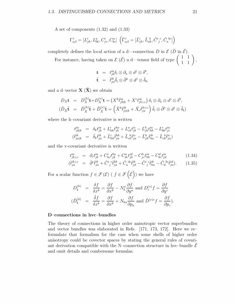
1.3. DISTINGUISHED CONNECTIONS AND METRICS 21
A set of components (1.32) and (1.33)
Γγαβ = [Li
jk, Labk, C
ijc, C
abc](Γγ
αβ = [Lijk, L
bak, C
i cj , C
bca ])
completely defines the local action of a d—connection D in E (D in E).For instance, having taken on E (E) a d—tensor field of type
(1 11 1
),
t = tiajbδi ⊗ ∂a ⊗ dj ⊗ δb,
t = tibjaδi ⊗ ∂a ⊗ dj ⊗ δb,
and a d–vector X (X) we obtain
DXt = D(h)X t+D
(v)X t =
(Xktiajb|k +Xctiajb⊥c
)δi ⊗ ∂a ⊗ dj ⊗ δb,
(DX t = D(h)
Xt + D
(v)
Xt =
(Xktibja|k + Xct
ib⊥cja
)δi ⊗ ∂a ⊗ dj ⊗ δb)
where the h–covariant derivative is written
tiajb|k = δktiajb + Li
hkthajb + La
ckticjb − Lh
jktiahb − Lc
bktiajc
(tibja|k = δk tibja + Li
hk thbja + L b
ckticja − Lh
jk tibha − L b
ckticja)
and the v-covariant derivative is written
tiajb⊥c = ∂ctiajb + Ci
hcthajb + Ca
dctidjb − Ch
jctiahb − Cd
bctiajd (1.34)
(tib⊥cja = ∂ctibja + Ci c
j thbja + C dc
a tibjd − Ci cj t
ibha − C bc
d tidja). (1.35)
For a scalar function f ∈ F (E) ( f ∈ F(E)) we have
D(h)k =
δf
δxk=
∂f
∂xk−Na
k
∂f
∂yaand D(v)
c f =∂f
∂yc
(D(h)k =
δf
δxk=
∂f
∂xk+Nka
∂f
∂paand D(v)cf =
∂f
∂pc).
D–connections in hvc–bundles
The theory of connections in higher order anisotropic vector superbundlesand vector bundles was elaborated in Refs. [171, 173, 172]. Here we re–formulate that formalism for the case when some shells of higher orderanisotropy could be covector spaces by stating the general rules of covari-ant derivation compatible with the N–connection structure in hvc–bundle Eand omit details and combersome formulas.

22 CHAPTER 1. VECTOR BUNDLES AND N–CONNECTIONS
For a hvc–bundle of type E = E [v(1), v(2), cv(3), ..., cv(z − 1), v(z)] a d–connection Γγ
αβ has the next shell decomposition of components (on inductionbeing on the p-th shell, considered as the base space, which in this case ahvc–bundle, we introduce in a usual manner, like a vector or covector fibre,the (p+ 1)-th shell)
Γγαβ = Γγ1
α1β1= [Li1
j1k1, La1
b1k1, Ci1
j1c1, Ca1
b1c1],
Γγ2
α2β2= [Li2
j2k2, La2
b2k2, Ci2
j2c2, Ca2
b2c2],
Γγ3
α3β3= [Li3
j3k3, L b3
a3k3, Ci3 c3
j3, C b3c3
a3],
....................................,
Γγz−1
αz−1βz−1= [L
iz−1
jz−1kz−1, L
bz−1
az−1kz−1, C
iz−1 cz−1
jz−1, C bz−1cz−1
az−1],
Γγz
αzβz= [Liz
jzkz, Laz
bzkz, Ciz
jzcz, Caz
bzcz].
These coefficients determine the rules of a covariant derivation D on E .For example, let us consider a d–tensor t of type(
1 11 12 13 ... 1z
1 11 12 13 ... 1z
)with corresponding tensor product of components of anholonomic N–frames(1.22) and (1.24)
t = tia1a2 b3...bz−1az
jb1b2a3...az−1bzδi ⊗ ∂a1 ⊗ dj ⊗ δb1 ⊗ ∂a2 ⊗ δb2 ⊗ ∂a3 ⊗ δb3 ,
...⊗ ∂az−1 ⊗ δbz−1 ⊗ ∂az ⊗ δbz .
The d–covariant derivation D of t is to be performed separately for everyshall according the rule (1.34) if a shell is defined by a vector subspace, oraccording the rule (1.35) if the shell is defined by a covector subspace.
1.3.2 Metric structure
D–metrics in v–bundles
We define a metric structure G in the total space E of a v–bundle E =(E, p,M) over a connected and paracompact base M as a symmetric covari-ant tensor field of type (0, 2),
G = Gαβduα ⊗ duβ
being non degenerate and of constant signature on E.

1.3. DISTINGUISHED CONNECTIONS AND METRICS 23
Nonlinear connection N and metric G structures on E are mutually com-patible it there are satisfied the conditions:
G (δi, ∂a) = 0, or equivalently, Gia (u)−N bi (u)hab (u) = 0, (1.36)
where hab = G (∂a, ∂b) and Gia = G (∂i, ∂a) , which gives
N bi (u) = hab (u)Gia (u) (1.37)
( the matrix hab is inverse to hab). In consequence one obtains the followingdecomposition of metric:
G(X, Y )= hG(X, Y ) + vG(X, Y ), (1.38)
where the d–tensor hG(X, Y )= G(hX, hY ) is of type
(0 02 0
)and the
d–tensor vG(X, Y ) = G(vX, vY ) is of type
(0 00 2
). With respect to an-
holonomic basis (1.16) the d–metric (1.38) is written
G = gαβ (u) δα ⊗ δβ = gij (u) di ⊗ dj + hab (u) δa ⊗ δb, (1.39)
where gij = G (δi, δj) .A metric structure of type (1.38) (equivalently, of type (1.39)) or a metric
on E with components satisfying constraints (1.36), (equivalently (1.37))defines an adapted to the given N–connection inner (d–scalar) product onthe tangent bundle T E .
We shall say that a d–connection DX is compatible with the d-scalarproduct on T E (i. e. it is a standard d–connection) if
DX (X ·Y) =(DXY
)· Z + Y·
(DXZ
), ∀X,Y,Z∈X (E).
An arbitrary d–connection DX differs from the standard one DX by an oper-ator PX (u) = XαP γ
αβ (u), called the deformation d-tensor with respect to
DX , which is just a d-linear transform of Eu, ∀ u ∈ E . The explicit form of PX
can be found by using the corresponding axiom defining linear connections[91] (
DX − DX
)fZ = f
(DX − DX
)Z,
written with respect to N–elongated bases (1.16) and (1.17). From the lastexpression we obtain
PX (u) =[(DX − DX)δα (u)
]δα (u) ,

24 CHAPTER 1. VECTOR BUNDLES AND N–CONNECTIONS
therefore
DXZ = DXZ +PXZ. (1.40)
A d–connection DX is metric (or compatible with metric G) on E if
DXG = 0, ∀X∈X (E).
With respect to anholonomic frames these conditions are written
Dαgβγ = 0, (1.41)
where by gβγ we denote the coefficients in the block form (1.39).
D–metrics in cv– and hvc–bundles
The presented considerations on self–consisten definition of N–connection,d–connection and metric structures in v–bundles can reformulated in a sim-ilar fashion for another types of anisotropic space–times, on cv–bundles andon shells of hvc–bundles. For symplicity, we give here only the anagolousformulas for the metric d–tensor (1.39):
• On cv–bundle E we write
G = gαβ (u) δα ⊗ δβ = gij (u) di ⊗ dj + hab (u) δa ⊗ δb, (1.42)
where gij = G(δi, δj
)and hab = G
(∂a, ∂b
)and the N–coframes are
given by formulas (1.20).
For simplicity, we shall consider that the metricity conditions are sat-isfied, Dγ gαβ = 0.
• On hvc–bundle E we write
G = gαβ (u) δα ⊗ δβ = gij (u) di ⊗ dj + ha1b1 (u) δa1 ⊗ δb1 (1.43)
+ha2b2 (u) δa2 ⊗ δb2 + ha3b3 (u) δa3 ⊗ δb3 + ...
+haz−1bz−1 (u) δaz−1 ⊗ δbz−1 + hazbz (u) δaz ⊗ δbz ,
where gij = G(δi, δj
)and ha1b1 = G (∂a1 , ∂b1) , ha2b2 = G (∂a2 , ∂b2) ,
ha3b3 = G(∂a3 , ∂b3
), .... and the N–coframes are given by formulas
(1.24).
The metricity conditions are Dγ gαβ = 0.

1.3. DISTINGUISHED CONNECTIONS AND METRICS 25
• On osculator bundle T 2M = Osc2M we have a particular case of (1.43)when
G = gαβ (u) δα ⊗ δβ (1.44)
= gij (u) di ⊗ dj + hij (u) δyi(1) ⊗ δyi
(1) + hij (u) δyi(2) ⊗ δyi
(2)
where the N–coframes are given by (1.27).
• On dual osculator bundle (T ∗2M, p∗2,M) we have another particularcase of (1.43) when
G = gαβ (u) δα ⊗ δβ (1.45)
= gij (u) di ⊗ dj + hij (u) δyi(1) ⊗ δyi
(1) + hij (u) δp(2)i ⊗ δp
(2)i
where the N–coframes are given by (1.28).
1.3.3 Some remarkable d–connections
We emphasize that the geometry of connections in a v–bundle E is very reach.If a triple of fundamental geometric objects
(Na
i (u) ,Γαβγ (u) , gαβ (u)
)is fixed
on E , a multi–connection structure (with corresponding different rules of co-variant derivation, which are, or not, mutually compatible and with the same,or not, induced d–scalar products in T E) is defined on this v–bundle. We cangive a priority to a connection structure following some physical arguments,like the reduction to the Christoffel symbols in the holonomic case, mutualcompatibility between metric and N–connection and d–connection structuresand so on.
In this subsection we enumerate some of the connections and covariantderivations in v–bundle E , cv–bundle E and in some hvc–bundles which canpresent interest in investigation of locally anisotropic gravitational and mat-ter field interactions :
1. Every N–connection in E with coefficients Nai (x, y) being differentiable
on y–variables, induces a structure of linear connection Nαβγ, where
Nabi =
∂Nai
∂yband Na
bc (x, y) = 0. (1.46)
For some Y (u) = Y i (u) ∂i +Y a (u) ∂a and B (u) = Ba (u) ∂a one intro-duces a covariant derivation as
D(N)Y B =
[Y i
(∂Ba
∂xi+Na
biBb
)+ Y b∂B
a
∂yb
]∂
∂ya.

26 CHAPTER 1. VECTOR BUNDLES AND N–CONNECTIONS
2. The d–connection of Berwald type [32] on v–bundle E (cv–bundle E)
Γ(B)αβγ =
(Li
jk,∂Na
k
∂yb, 0, Ca
bc
), (1.47)
(Γ(B)αβγ =
(Li
jk,−∂Nka
∂pb, 0, C bc
a
))
where
Li.jk (x, y) =
1
2gir
(δgjk
δxk+δgkr
δxj− δgjk
δxr
), (1.48)
Ca.bc (x, y) =
1
2had
(∂hbd
∂yc+∂hcd
∂yb− ∂hbc
∂yd
)(Li
.jk (x, p) =1
2gir
(δgjk
δxk+δgkr
δxj− δgjk
δxr
),
C bca (x, p) =
1
2had
(∂hbd
∂pc+∂hcd
∂pb− ∂hbc
∂pd
)),
which is hv—metric, i.e. there are satisfied the conditions D(B)k gij = 0
and D(B)c hab = 0 (D
(B)k gij = 0 and D(B)chab = 0).
3. The canonical d–connection Γ(c) (or Γ(c)) on a v–bundle (or cv–bundle)is associated to a metric G (or G) of type (1.39) (or (1.42)),
Γ(c)αβγ = [L
(c)ijk , L
(c)abk , C
(c)ijc , C
(c)abc ] (Γ
(c)αβγ = [L
(c)ijk , L
(c).ba .k, C
(c)i cj , C(c) bc
a ])
with coefficients
L(c)ijk = Li
.jk, C(c)abc = Ca
.bc (L(c)ijk = Li
.jk, C(c) bca = C bc
a ), (see (1.48)
L(c)abi =
∂Nai
∂yb+
1
2hac
(δhbc
δxi− ∂Nd
i
∂ybhdc −
∂Ndi
∂ychdb
)(L
(c).ba .i = −∂N
ai
∂pb+
1
2hac
(δhbc
δxi+∂Nid
∂pbhdc +
∂Nid
∂pchdb
)),
C(c)ijc =
1
2gik∂gjk
∂yc(C
(c)i cj =
1
2gik∂gjk
∂pc
). (1.49)
This is a metric d–connection which satisfies conditions
D(c)k gij = 0, D(c)
c gij = 0, D(c)k hab = 0, D(c)
c hab = 0
(D(c)k gjk = 0, D(c)cgjk = 0, D
(c)k hbc = 0, D(c)chab = 0).

1.3. DISTINGUISHED CONNECTIONS AND METRICS 27
In physical applications we shall use the canonical connection and forsymplicity we chall omit the index (c). The coefficients (1.49) are to beextended to higher order if we are dealing with derivations of geomet-rical objects with ”shell” indices. In this case the fiber indices are tobe stipulated for every type of shell into consideration.
4. We can consider the N–adapted Christoffel d–symbols
Γαβγ =
1
2gατ (δγgτβ + δβgτγ − δgβγ) , (1.50)
which have the components of d–connection Γαβγ =
(Li
jk, 0, 0, Cabc
), with
Lijk and Ca
bc as in (1.48) if gαβ is taken in the form (1.39).
Arbitrary linear connections on a v-bundle E can be also characterizedby theirs deformation tensors (see (1.40)) with respect, for instance, to thed–connection (1.50):
Γ(B)αβγ = Γα
βγ + P(B)αβγ ,Γ
(c)αβγ = Γα
βγ + P(c)αβγ
or, in general,
Γαβγ = Γα
βγ + P αβγ,
where P(B)αβγ , P
(c)αβγ and P α
βγ are respectively the deformation d-tensors of d–connections (1.47), (1.49) or of a general one. Similar deformation d–tensorscan be introduced for d–connections on cv–bundles and hvc–bundles. Weomit explicit formulas.
1.3.4 Amost Hermitian anisotropic spaces
The are possible very interesting particular constructions [108, 109, 113] ont–bundle TM provided with N–connection which defines a N–adapted framestructure δα = (δi, ∂i) (for the same formulas (1.16) and (1.17) but withidentified fiber and base indices). We are using the ’dot’ symbol in order todistinguish the horizontal and vertical operators because on t–bundles theindices could take the same values both for the base and fiber objects. Thisallow us to define an almost complex structure J = J β
α on TM as follows
J(δi) = −∂i, J(∂i) = δi. (1.51)
It is obvious that J is well–defined and J2 = −I.

28 CHAPTER 1. VECTOR BUNDLES AND N–CONNECTIONS
For d–metrics of type (1.39), on TM, we can consider the case whengij(x, y) = hab(x, y), i. e.
G(t) = gij(x, y)dxi ⊗ dxj + gij(x, y)δy
i ⊗ δyj, (1.52)
where the index (t) denotes that we have geometrical object defined on tan-gent space.
An almost complex structure J βα is compatible with a d–metric of type
(1.52) and a d–connection D on tangent bundle TM if the conditions
J βα J δ
γ gβδ = gαγ and DαJγβ = 0
are satisfied.The pair (G(t),J) is an almost Hermitian structure on TM.One can introduce an almost sympletic 2–form associated to the almost
Hermitian structure (G(t),J),
θ = gij(x, y)δyi ∧ dxj. (1.53)
If the 2–form (1.53), defined by the coefficients gij, is closed, we obtainan almost Kahlerian structure in TM.
Definition 1.6. An almost Kahler metric connection is a linear connectionD(H) on TM = TM \ 0 with the properties:
1. D(H) preserve by parallelism the vertical distribution defined by the N–connection structure;
2. D(H) is compatible with the almost Kahler structure (G(t),J), i. e.
D(H)X g = 0, D
(H)X J = 0, ∀X ∈ X
(TM
).
By straightforward calculation we can prove that a d–connection DΓ =(Li
jk, Lijk, C
ijc, C
ijc
)with the coefficients defined by
D(H)δiδj = Li
jkδi, D(H)δi∂j = Li
jk∂i, (1.54)
D(H)δiδj = Ci
jkδi, D(H)δi∂j = Ci
jk∂i,
where Lijk and Ce
ab → Cijk, on TM are defined by the formulas (1.48), define
a torsionless (see the next section on torsion structures) metric d–connectionwhich satisfy the compatibility conditions (1.41).
Almost complex structures and almost Kahler models of Finsler, La-grange, Hamilton and Cartan geometries (of first an higher orders) are in-vestigated in details in Refs. [106, 107, 113, 172].

1.4. TORSIONS AND CURVATURES 29
1.4 Torsions and Curvatures
In this section we outline the basic definitions and formulas for the torsionand curvature structures in v–bundles and cv–bundles provided with N–connection structure.
1.4.1 N–connection curvature
1. The curvature Ω of a nonlinear connection N in a v–bundle E can bedefined in local form as [108, 109]:
Ω =1
2Ωa
ijdi∧
dj ⊗ ∂a,
where
Ωaij = δjN
ai − δiNa
j (1.55)
= ∂jNai − ∂iN
aj +N b
iNabj −N b
jNabi,
Nabi being that from (1.46).
2. For the curvature Ω, of a nonlinear connection N in a cv–bundle E weintroduce
Ω =1
2Ωijad
i∧
dj ⊗ ∂a,
where
Ωija = −δjNia + δiNja (1.56)
= −∂jNia + ∂iNja + NibNb
ja − NjbNb
ja ,
N bja = ∂bNja = ∂Nja/∂pb.
3. Curvatures Ω of different type of nonlinear connections N in higherorder anisotropic bundles were analyzed for different type of higherorder tangent/dual tangent bundles and higher order prolongations ofgeneralized Finsler, Lagrange and Hamiloton spaces in Refs. [106, 107,113] and for higher order anisotropic superspaces and spinor bundles inRefs. [172, 165, 173, 171]: For every higher order anisotropy shell weshall define the coefficients (1.55) or (1.56) in dependence of the factwith type of subfiber we are considering (a vector or covector fiber).

30 CHAPTER 1. VECTOR BUNDLES AND N–CONNECTIONS
1.4.2 d–Torsions in v- and cv–bundles
The torsion T of a d–connection D in v–bundle E (cv–bundle E) is definedby the equation
T (X,Y) = XYT
.=DXY−DY X − [X,Y] . (1.57)
One holds the following h- and v–decompositions
T (X,Y) = T (hX,hY) + T (hX,vY) + T (vX,hY) + T (vX,vY) .
We consider the projections:
hT (X,Y) ,vT (hX,hY) ,hT (hX,hY) , ...
and say that, for instance, hT (hX,hY) is the h(hh)–torsion of D ,vT (hX,hY) is the v(hh)–torsion of D and so on.
The torsion (1.57) in v-bundle is locally determined by five d–tensor fields,torsions, defined as
T ijk = hT (δk, δj) · di, T a
jk = vT (δk, δj) · δa, (1.58)
P ijb = hT (∂b, δj) · di, P a
jb = vT (∂b, δj) · δa,
Sabc = vT (∂c, ∂b) · δa.
Using formulas (1.16), (1.17), (1.55) and (1.57) we can computer [108, 109]in explicit form the components of torsions (1.58) for a d–connection of type(1.32) and (1.33):
T i.jk = T i
jk = Lijk − Li
kj, T ija = Ci
.ja, Tiaj = −Ci
ja, (1.59)
T i.ja = 0, T a
.bc = Sa.bc = Ca
bc − Cacb,
T a.ij = δjN
ai − δjNa
j , T a.bi = P a
.bi = ∂bNai − La
.bj , T a.ib = −P a
.bi.
Formulas similar to (1.58) and (1.59) hold for cv–bundles:
T ijk = hT (δk, δj) · di, Tjka = vT (δk, δj) · δa, (1.60)
P i bj = hT
(∂b, δj
)· di, P b
aj = vT(∂b, δj
)· δa,
S bca = vT
(∂c, ∂b
)· δa.
and
T i.jk = T i
jk = Lijk − Li
kj, T iaj = Ci a
.j , T iaj = −Ci a
j , (1.61)
T i a.j = 0, T bc
a = S bca = C bc
a − C cba ,
T.ija = −δjNia + δjNja, T bia = P bi
a = −∂bNia − L bia , T j
a b = −P ja b.
The formulas for torsion can be generalized for hvc–bundles (on everyshell we must write (1.59) or (1.61) in dependence of the type of shell, vectoror co-vector one, we are dealing).

1.4. TORSIONS AND CURVATURES 31
1.4.3 d–Curvatures in v- and cv–bundles
The curvature R of a d–connection in v–bundle E is defined by the equation
R (X, Y )Z = XY •• R • Z = DXDY Z −DYDXZ −D[X,Y ]Z.
One holds the next properties for the h- and v–decompositions of curvature:
vR (X, Y ) hZ = 0, hR (X, Y ) vZ = 0, (1.62)
R (X, Y )Z = hR (X, Y )hZ + vR (X, Y ) vZ.
From (1.62) and the equation R (X,Y) = −R (Y,X) we get that thecurvature of a d–connection D in E is completely determined by the followingsix d–tensor fields:
R.ih.jk = di ·R (δk, δj) δh, R
.ab.jk = δa ·R (δk, δj) ∂b, (1.63)
P .ij.kc = di ·R (∂c, ∂k) δj , P
.ab.kc = δa ·R (∂c, ∂k) ∂b,
S .ij.bc = di ·R (∂c, ∂b) δj, S
.ab.cd = δa ·R (∂d, ∂c) ∂b.
By a direct computation, using (1.16),(1.17),(1.32),(1.33) and (1.63) we get:
R.ih.jk = δhL
i.hj − δjLi
.hk + Lm.hjL
imk − Lm
.hkLimj + Ci
.haRa.jk, (1.64)
R.ab.jk = δkL
a.bj − δjLa
.bk + Lc.bjL
a.ck − Lc
.bkLa.cj + Ca
.bcRc.jk,
P .ij.ka = ∂aL
i.jk −
(δkC
i.ja + Li
.lkCl.ja − Ll
.jkCi.la − Lc
.akCi.jc
)+ Ci
.jbPb.ka,
P .cb.ka = ∂aL
c.bk −
(δkC
c.ba + Lc
.dkCd.ba − Ld
.bkCc.da − Ld
.akCc.bd
)+ Cc
.bdPd.ka,
S .ij.bc = ∂cC
i.jb − ∂bC
i.jc + Ch
.jbCi.hc − Ch
.jcCihb,
S .ab.cd = ∂dC
a.bc − ∂cC
a.bd + Ce
.bcCa.ed − Ce
.bdCa.ec.
We note that d–torsions (1.59) and d–curvatures (1.64) are computed inexplicit form by particular cases of d–connections (1.47), (1.49) and (1.50).
For cv–bundles we have
R.ih.jk = di ·R (δk, δj) δh, R
ba.jk = δa ·R (δk, δj) ∂
b, (1.65)
P .i cj.k = di ·R
(∂c, ∂k
)δj , P
b ca.k = δa ·R
(∂c, ∂k
)∂b,
S .ibcj. = di ·R
(∂c, ∂b
)δj , S
b.cd.a = δa ·R
(∂d, ∂c
)∂b.

32 CHAPTER 1. VECTOR BUNDLES AND N–CONNECTIONS
and
R.ih.jk = δhL
i.hj − δjLi
.hk + Lm.hjL
imk − Lm
.hkLimj + Ci a
.h R.ajk, (1.66)
Rb..ajk = δkL
ba.j − δjLa
b k + L bcjL
c.ak − Lb
ckLc
a.j + C bca Rc.jk,
P .i aj.k = ∂aLi
.jk −(δkC
i a.j + Li
.lkCl a.j − Ll
.jkCi a.l − L a
ckCi c.j
)+ Ci b
.j Pa
bk ,
P b ack = ∂aL b
c.k − (δkCba
c. + Lbdc.kC
bad − L b
d.k Cad
c. ),
−L adk C bd
c. ) + C bdc. P
ad.k ,
S .ibcj. = ∂cCi b
.j − ∂bCi c.j + Ch b
.j Ci c.h − Ch c
.j Ci bh ,
Sb cda. = ∂dC bc
a. − ∂cC bda. + C bc
e. Ced
a. − C bde. C
ec.a .
The formulas for curvature can be also generalized for hvc–bundles (onevery shell we must write (1.59) or (1.60) in dependence of the type of shell,vector or co-vector one, we are dealing).
1.5 Generalizations of Finsler Spaces
We outline the basic definitions and formulas for Finsler, Lagrange and gen-eralized Lagrange spaces (constructed on tangent bundle) and for Cartan,Hamilton and generalized Hamilton spaces (constructed on cotangent bun-dle). The original results are given in details in monographs [108, 109, 113]
1.5.1 Finsler Spaces
The Finsler geometry is modeled on tangent bundle TM.
Definition 1.7. A Finsler space (manifold) is a pair F n = (M,F (x, y))where M is a real n–dimensional differentiable manifold and F : TM → Ris a scalar function which satisfy the following conditions:
1. F is a differentiable function on the manifold TM = TM\0 and Fis continous on the null section of the projection π : TM →M ;
2. F is a positive function, homogeneous on the fibers of the TM, i. e.F (x, λy) = λF (x, y), λ ∈ R;
3. The Hessian of F 2 with elements
g(F )ij (x, y) =
1
2
∂2F 2
∂yi∂yj(1.67)
is positively defined on TM.

1.5. GENERALIZATIONS OF FINSLER SPACES 33
The function F (x, y) and gij(x, y) are called respectively the fundamentalfunction and the fundamental (or metric) tensor of the Finsler space F.
One considers ”anisotropic” (depending on directions yi) Christoffel sym-
bols, for simplicity we write g(F )ij = gij,
γijk(x, y) =
1
2gir
(∂grk
∂xj+∂gjr
∂xk− ∂gjk
∂xr
),
which are used for definition of the Cartan N–connection,
N i(c) j =
1
2
∂
∂yj
[γi
nk(x, y)ynyk]. (1.68)
This N–connection can be used for definition of an almost complex structurelike in (1.51) and to define on TM a d–metric
G(F ) = gij(x, y)dxi ⊗ dxj + gij(x, y)δy
i ⊗ δyj, (1.69)
with gij(x, y) taken as (1.67).
Using the Cartan N–connection (1.68) and Finsler metric tensor (1.67)(or, equivalently, the d–metric (1.69)) we can introduce the canonical d–connection
DΓ(N(c)
)= Γα
(c)βγ =(Li
(c) jk, Ci(c) jk
)with the coefficients computed like in (1.54) and (1.48) with hab → gij. Thed–connection DΓ
(N(c)
)has the unique property that it is torsionless and
satisfies the metricity conditions both for the horizontal and vertical compo-nents, i. e. Dαgβγ = 0.
The d–curvatures
R.ih.jk = R.i
h.jk, P.i lj.k , S .i
(c)j.kl
on a Finsler space provided with Cartan N–connection and Finsler metricstructures are computed following the formulas (1.64) when the a, b, c... in-dices are identified with i, j, k, ... indices. It should be emphasized that in thiscase all values gij,Γ
α(c)βγ and R.α
(c)β.γδ are defined by a fundamental function
F (x, y) .
In general, we can consider that a Finsler space is provided with a metricgij = ∂2F 2/2∂yi∂yj , but the N–connection and d–connection are be definedin a different manner, even not be determined by F.

34 CHAPTER 1. VECTOR BUNDLES AND N–CONNECTIONS
1.5.2 Lagrange and Generalized Lagrange Spaces
The notion of Finsler spaces was extended by J. Kern [86] and R. Miron [99].It is widely developed in monographs [108, 109] and exteded to superspacesby S. Vacaru [169, 171, 172].
The idea of extension was to consider instead of the homogeneous funda-mental function F (x, y) in a Finsler space a more general one, a LagrangianL (x, y), defined as a differentiable mapping L : (x, y) ∈ TM → L(x, y) ∈ R,of class C∞ on manifold TM and continous on the null section 0 : M → TMof the projection π : TM →M. A Lagrangian is regular if it is differentiableand the Hessian
g(L)ij (x, y) =
1
2
∂2L2
∂yi∂yj(1.70)
is of rank n on M.
Definition 1.8. A Lagrange space is a pair Ln = (M,L(x, y)) where Mis a smooth real n–dimensional manifold provided with regular LagrangianL(x, y) structure L : TM → R for which gij(x, y) from (1.70) has a constant
signature over the manifold TM.
The fundamental Lagrange function L(x, y) defines a canonical N–con-nection
N i(cL) j =
1
2
∂
∂yj
[gik
(∂2L2
∂yk∂yhyh − ∂L
∂xk
)]as well a d-metric
G(L) = gij(x, y)dxi ⊗ dxj + gij(x, y)δy
i ⊗ δyj, (1.71)
with gij(x, y) taken as (1.70). As well we can introduce an almost Kahlerianstructure and an almost Hermitian model of Ln, denoted as H2n as in thecase of Finsler spaces but with a proper fundamental Lagange function andmetric tensor gij. The canonical metric d–connection DΓ
(N(cL)
)= Γα
(cL)βγ =(Li
(cL) jk, Ci(cL) jk
)is to computed by the same formulas (1.54) and (1.48)
with hab → g(L)ij , for N i
(cL) j . The d–torsions (1.59) and d–curvatures (1.64)
are defined, in this case, by Li(cL) jk and Ci
(cL) jk. We also note that instead of
N i(cL) j and Γα
(cL)βγ one can consider on a Ln–space arbitrary N–connections
N ij , d–connections Γα
βγ which are not defined only by L(x, y) and g(L)ij but
can be metric, or non–metric with respect to the Lagrange metric.The next step of generalization is to consider an arbitrary metric gij (x, y)
on TM instead of (1.70) which is the second derivative of ”anisotropic” co-ordinates yi of a Lagrangian [99, 100].

1.5. GENERALIZATIONS OF FINSLER SPACES 35
Definition 1.9. A generalized Lagrange space is a pair GLn = (M, gij(x, y))where gij(x, y) is a covariant, symmetric d–tensor field, of rank n and of
constant signature on TM.
One can consider different classes of N– and d–connections on TM, whichare compatible (metric) or non compatible with (1.71) for arbitrary gij(x, y).We can apply all formulas for d–connections, N-curvatures, d-torsions andd-curvatures as in a v–bundle E , but reconsidering them on TM, by changinghab → gij(x, y) and Na
i → Nki.
1.5.3 Cartan Spaces
The theory of Cartan spaces (see, for instance, [136, 85]) was formulated ina new fashion in R. Miron’s works [101, 102] by considering them as dualsto the Finsler spaces (see details and references in [113]). Roughly, a Cartanspace is constructed on a cotangent bundle T ∗M like a Finsler space on thecorresponding tangent bundle TM.
Consider a real smooth manifold M, the cotangent bundle (T ∗M,π∗,M)
and the manifold T ∗M = T ∗M\0.
Definition 1.10. A Cartan space is a pair Cn = (M,K(x, p)) such thatK : T ∗M →R is a scalar function which satisfy the following conditions:
1. K is a differentiable function on the manifold T ∗M = T ∗M\0 andcontinous on the null section of the projection π∗ : T ∗M →M ;
2. K is a positive function, homogeneous on the fibers of the T ∗M, i. e.K(x, λp) = λF (x, p), λ ∈ R;
3. The Hessian of K2 with elements
gij(K)(x, p) =
1
2
∂2K2
∂pi∂pj
(1.72)
is positively defined on T ∗M.
The functionK(x, y) and gij(x, p) are called respectively the fundamentalfunction and the fundamental (or metric) tensor of the Cartan space Cn. Weuse symbols like ”g” as to emphasize that the geometrical objects are definedon a dual space.

36 CHAPTER 1. VECTOR BUNDLES AND N–CONNECTIONS
One considers ”anisotropic” (depending on directions, momenta, pi)
Christoffel symbols, for symplicty, we write the inverse to (1.72) as g(K)ij = gij,
γijk(x, p) =
1
2gir
(∂grk
∂xj+∂gjr
∂xk− ∂gjk
∂xr
),
which are used for definition of the canonical N–connection,
Nij = γkijpk −
1
2γk
nlpkpl∂ngij , ∂
n =∂
∂pn
. (1.73)
This N–connection can be used for definition of an almost complex structurelike in (1.51) and to define on T ∗M a d–metric
G(k) = gij(x, p)dxi ⊗ dxj + gij(x, p)δpi ⊗ δpj , (1.74)
with gij(x, p) taken as (1.72).Using the canonical N–connection (1.73) and Finsler metric tensor (1.72)
(or, equivalently, the d–metric (1.74) we can introduce the canonical d–connection
DΓ(N(k)
)= Γα
(k)βγ =(H i
(k) jk, Cjk
(k) i
)with the coefficients are computed
H i(k) jk =
1
2gir(δj grk + δkgjr − δr gjk
),
C jk(k) i = gis∂
sgjk,
The d–connection DΓ(N(k)
)has the unique property that it is torsionless
and satisfies the metricity conditions both for the horizontal and verticalcomponents, i. e. Dαgβγ = 0.
The d–curvatures
R.α(k)β.γδ = R.i
(k)h.jk, P.i(k)j.km, S
.iklj.
on a Finsler space provided with Cartan N–connection and Finsler metricstructures are computed following the formulas (1.66) when the a, b, c... in-dices are identified with i, j, k, ... indices. It should be emphasized that in thiscase all values gij,Γ
α(k)βγ and R.α
(k)β.γδ are defined by a fundamental function
K (x, p) .In general, we can consider that a Cartan space is provided with a met-
ric gij = ∂2K2/2∂pi∂pj , but the N–connection and d–connection could bedefined in a different manner, even not be determined by K.

1.5. GENERALIZATIONS OF FINSLER SPACES 37
1.5.4 Generalized Hamilton and Hamilton Spaces
The geometry of Hamilton spaces was defined and investigated by R. Mironin the papers [105, 104, 103] (see details and references in [113]). It wasdeveloped on the cotangent bundel as a dual geometry to the geometry ofLagrange spaces. Here we start with the definition of generalized Hamiltonspaces and then consider the particular case.
Definition 1.11. A generalized Hamilton space is a pairGHn = (M, gij(x, p)) where M is a real n–dimensional manifold and gij(x, p)is a contravariant, symmetric, nondegenerate of rank n and of constant sig-
nature on T ∗M.
The value gij(x, p) is called the fundamental (or metric) tensor of thespace GHn. One can define such values for every paracompact manifold M.In general, a N–connection on GHn is not determined by gij. Therefore wecan consider arbitrary coefficients Nij (x, p) and define on T ∗M a d–metriclike (1.42)
G = gαβ (u) δα ⊗ δβ = gij (u) di ⊗ dj + gij (u) δi ⊗ δj , (1.75)
This N–coefficients Nij (x, p) and d–metric structure (1.75) allow to define analmost Kahler model of generalized Hamilton spaces and to define canonicald–connections, d–torsions and d-curvatures (see respectively the formulas(1.48), (1.49), (1.61) and (1.64) with the fiber coefficients redefined for thecotangent bundle T ∗M ).
A generalized Hamilton space GHn = (M, gij(x, p)) is called reducible toa Hamilton one if there exists a Hamilton function H (x, p) on T ∗M suchthat
gij(x, p) =1
2
∂2H
∂pi∂pj
. (1.76)
Definition 1.12. A Hamilton space is a pair Hn = (M,H(x, p)) such thatH : T ∗M →R is a scalar function which satisfy the following conditions:
1. H is a differentiable function on the manifold T ∗M = T ∗M\0 andcontinous on the null section of the projection π∗ : T ∗M →M ;
2. The Hessian of H with elements (1.76) is positively defined on T ∗M andgij(x, p) is nondegenerate matrix of rank n and of constant signature.

38 CHAPTER 1. VECTOR BUNDLES AND N–CONNECTIONS
For Hamilton spaces the canonical N–connection (defined by H and itsHessian) exists,
Nij =1
4gij, H −
1
2
(gik
∂2H
∂pk∂xj+ gjk
∂2H
∂pk∂xi
),
where the Poisson brackets, for arbitrary functions f and g on T ∗M, act as
f, g =∂f
∂pi
∂g
∂xi− ∂g
∂pi
∂p
∂xi.
The canonical d–connection DΓ(N(c)
)= Γα
(c)βγ =(H i
(c) jk, Cjk
(c) i
)is de-
fined by the coefficients
H i(c) jk =
1
2gis(δj gsk + δkgjs − δsgjk
),
C jk(c) i = −1
2gis∂
j gsk.
In result we can compute the d–torsions and d–curvatures like on cv–bundleor on Cartan spaces. On Hamilton spaces all such objects are defined by theHamilton function H(x, p) and indeces have to be reconsidered for co–fibersof the co-tangent bundle.
1.6 Gravity on Vector Bundles
The components of the Ricci d–tensor
Rαβ = R.τα.βτ
with respect to a locally adapted frame (1.17) are as follows:
Rij = R.ki.jk, Ria = −2Pia = −P .k
i.ka, (1.77)
Rai = 1Pai = P .ba.ib, Rab = S .c
a.bc.
We point out that because, in general, 1Pai 6= 2Pia the Ricci d-tensor is nonsymmetric.
Having defined a d-metric of type in E we can introduce the scalar cur-vature of d–connection D:
←−R = GαβRαβ = R+ S, (1.78)
where R = gijRij and S = habSab.

1.6. GRAVITY ON VECTOR BUNDLES 39
For our further considerations it will be also useful to use an alternativeway of definition torsion (1.57) and curvature (1.62) by using the commutator
∆αβ.= 5α5β −5β 5α = 25[α5β].
For components of d–torsion we have
∆αβf = T γ.αβ 5γ f
for every scalar function f on E . Curvature can be introduced as an operatoracting on arbitrary d-vector V δ :
(∆αβ − T γ.αβ5γ)V
δ = R.δγ.αβV
γ (1.79)
(we note that in this section we shall follow conventions of Miron and Anas-tasiei [108, 109] on d-tensors; we can obtain corresponding Penrose andRindler abstract index formulas [128, 129] just for a trivial N-connectionstructure and by changing denotations for components of torsion and curva-ture in this manner: T γ
.αβ → T γαβ and R.δ
γ.αβ → R δαβγ ).
Here we also note that torsion and curvature of a d-connection on Esatisfy generalized for locally anisotropic spaces Ricci and Bianchi identities[108, 109] which in terms of components (1.79) are written respectively as
R.δ[γ.αβ] +5[αT
δ.βγ] + T ν
.[αβTδ.γ]ν = 0 (1.80)
and
5[αR·σ|ν|βγ] + T δ
·[αβR·σ|ν|.γ]δ = 0. (1.81)
Identities (1.80) and (1.81) can be proved similarly as in [128] by taking intoaccount that indices play a distinguished character.
We can also consider a la-generalization of the so-called conformal Weyltensor (see, for instance, [128]) which can be written as a d-tensor in thisform:
Cγδαβ = Rγδ
αβ −4
n+m− 2R
[γ[α δ
δ]β] (1.82)
+2
(n+m− 1)(n+m− 2)
←−R δ
[γ[α δ
δ]β].
This object is conformally invariant on locally anisotropic spaces providedwith d-connection generated by d-metric structures.
The Einstein equations and conservation laws on v-bundles provided withN-connection structures are studied in detail in [108, 109, 2, 3]. In Ref. [186]

40 CHAPTER 1. VECTOR BUNDLES AND N–CONNECTIONS
we proved that the locally anisotropic gravity can be formulated in a gaugelike manner and analyzed the conditions when the Einstein locally anisotropicgravitational field equations are equivalent to a corresponding form of Yang-Mills equations. In this subsection we write the locally anisotropic gravita-tional field equations in a form more convenient for theirs equivalent refor-mulation in locally anisotropic spinor variables.
We define d-tensor Φαβ as to satisfy conditions
−2Φαβ.= Rαβ −
1
n +m
←−R gαβ (1.83)
which is the torsionless part of the Ricci tensor for locally isotropic spaces[128, 129], i.e. Φ α
α.= 0. The Einstein equations on locally anisotropic spaces
←−G αβ + λgαβ = κEαβ, (1.84)
where
←−G αβ = Rαβ −
1
2
←−R gαβ (1.85)
is the Einstein d-tensor, λ and κ are correspondingly the cosmological andgravitational constants and by Eαβ is denoted the locally anisotropic energy-momentum d-tensor [108, 109], can be rewritten in equivalent form:
Φαβ = −κ2(Eαβ −
1
n+mE τ
τ gαβ). (1.86)
Because the locally anisotropic spaces generally have nonzero torsions weshall add to (1.86) (equivalently to (1.84)) a system of algebraic d-field equa-tions with the source Sα
βγ being the locally anisotropic spin density of matter(if we consider a variant of locally anisotropic Einstein-Cartan theory):
T γαβ + 2δγ
[αTδβ]δ = κSγ
αβ. (1.87)
From (1.80) and (1.87) one follows the conservation law of locally anisotropicspin matter:
5γSγαβ − T δ
δγSγαβ = Eβα − Eαβ.
Finally, in this section, we remark that all presented geometric construc-tions contain those elaborated for generalized Lagrange spaces [108, 109] (forwhich a tangent bundle TM is considered instead of a v-bundle E ). Wealso note that the Lagrange (Finsler) geometry is characterized by a metric
with components parametized as gij = 12
∂2L∂yi∂yj
(gij = 1
2∂2Λ2
∂yi∂yj
)and hij = gij,
where L = L (x, y) (Λ = Λ (x, y)) is a Lagrangian (Finsler metric) on TM(see details in [108, 109, 96, 27]).

Chapter 2
Anholonomic Einstein andGauge Gravity
We analyze local anisotropies induced by anholonomic frames and associatednonlinear connections in general relativity and extensions to affine–Poincareand de Sitter gauge gravity and different types of Kaluza–Klein theories. Weconstruct some new classes of cosmological solutions of gravitational fieldequations describing Friedmann–Robertson–Walker like universes with rota-tion (ellongated and flattened) ellipsoidal or torus symmetry [185].
2.1 Introduction
The search for exact solutions with generic local anisotropy in general rela-tivity, gauge gravity and non–Riemannian extensions has its motivation fromlow energy limits in modern string and Kaluza–Klein theories. Such classesof solutions constructed by using moving anholonomic frame fields (tetrads,or vierbeins; we shall use the term frames for higher dimensions) reflect a newtype of constrained dynamics and locally anisotropic interactions of gravita-tional and matter fields [177].
What are the requirements of such constructions and their physical treat-ment? We believe that such solutions should have the properties: (i) theysatisfy the Einstein equations in general relativity and are locally anisotropicgeneralizations of some known solutions in isotropic limits with a well posedCauchy problem; (ii) the corresponding geometrical and physical values aredefined, as a rule, with respect to an anholonomic system of reference whichreflects the imposed constraints and supposed symmetry of locally anisotropicinteractions; the reformulation of results for a coordinate frame is also pos-sible; (iii) by applying the method of moving frames of reference, we can
41
42 CHAPTER 2. ANHOLONOMIC EINSTEIN AND GAUGE GRAVITY
generalize the solutions to some analogous in metric–affine and/or gaugegravity, in higher dimension and string theories.
Comparing with the previos results [163, 170, 173, 172, 186] on definitionof self–consistent field theories incorporating various possible anisotropic,inhomogeneous and stochastic manifestations of classical and quantum in-teractions on locally anisotropic and higher order anisotropic spaces, we em-phasize that, in this Chapter, we shall be interested not in some extensions ofthe well known gravity theories with locally isotropic space–times ((pseudo)Riemannian or Riemanian–Cartan–Weyl ones, in brief, RCW space–times)to Finsler geometry and its generalizations. We shall present a proof thatlocally anisotropic structures (Finsler, Lagrange and higher order develop-ments [59, 41, 136, 96, 14, 109, 106, 27, 70]) could be induced by anholonomicframes on locally isotropic spaces, even in general relativity and its metric–affine and gauge like modifications [63, 153, 132, 133, 98, 53, 186, 131, 202].
To evolve some new (frame anholonomy) features of locally isotropic grav-ity theories we shall apply the methods of the geometry of anholonomicframes and associated nonlinear connection (in brief, N–connection) struc-tures elaborated in details for bundle spaces and generalized Finsler spaces inmonographs [109, 106, 27] with further developments for spinor differentialgeometry, superspaces and stochastic calculus in [163, 171, 173, 172]. Thefirst rigorous global definition of N–connections is due to W. Barthel [25]but the idea and some rough constructions could be found in the E. Cartan’sworks [41]. We note that the point of this paper is to emphasize the generic lo-cally anisotropic geometry and physics and apply the N–connection methodfor ´non–Finslerian´(pseudo) Riemannian and RCW spacetimes. Here, itshould be mentioned that anholonomic frames are considered in detail, for in-stance, in monographs [56, 117, 128, 129] and with respect to geometrizationof gauge theories in [98, 131] but not concerning the topic on associated N–connection structures which grounds our geometric approach to anisotropiesin physical theories and developing of a new method of integrating gravita-tional field equations.
2.2 Anholonomic Frames on (Pseudo) Rie-
mannian Spaces
For definiteness, we consider a (n+m)–dimensional (pseudo) Riemannianspacetime V (n+m), being a paracompact and connected Hausdorff C∞–mani-fold, enabled with a nonsigular metric
ds2 = gαβ duα ⊗ duβ

2.2. ANHOLONOMIC FRAMES 43
with the coefficients
gαβ =
[gij +Na
i Nbjhab N e
j hae
N ei hbe hab
](2.1)
parametrized with respect to a local coordinate basis duα = (dxi, dya) ,having its dual ∂/uα = (∂/xi, ∂/ya) , where the indices of geometrical ob-jects and local coordinate uα =
(xk, ya
)run correspondingly the values: (for
Greek indices)α, β, . . . = n +m; for (Latin indices) i, j, k, ... = 1, 2, ..., n anda, b, c, ... = 1, 2, ..., m . We shall use ’tilds’ if would be necessary to emphasizethat a value is defined with respect to a coordinate basis.
The metric (2.1) can be rewritten in a block (n× n) + (m×m) form
gαβ =
(gij(x
k, ya) 00 hab(x
k, ya)
)(2.2)
with respect to a subclass of n+m anholonomic frame basis (for four dimen-sions one used terms tetrads, or vierbiends) defined
δα = (δi, ∂a) =δ
∂uα=
(δi =
δ
∂xi=
∂
∂xi−N b
i
(xj , yc
) ∂
∂yb, ∂a =
∂
∂ya
)(2.3)
and
δβ =(di, δa
)= δuβ =
(di = dxi, δa = δya = dya +Na
k
(xj , yb
)dxk), (2.4)
called the locally anisotropic bases (in brief, la–bases) adapted to the coef-ficients Na
j . The n× n matrix gij defines the so–called horizontal metric (inbrief, h–metric) and the m × m matrix hab defines the vertical (v–metric)with respect to the associated nonlinear connection (N–connection) struc-ture given by its coefficients Na
j (uα) from (2.3) and (2.4). The geometryof N–connections is studied in detail in [25, 109]; here we shall consider itsapplications with respect to anholonomic frames in general relativity and itslocally isotropic generalizations.
A frame structure δα (2.3) on V (n+m) is characterized by its anholonomyrelations
δαδβ − δβδα = wγαβδγ. (2.5)
with anholonomy coefficients wαβγ.The elongation of partial derivatives (by
N–coefficients) in the locally adapted partial derivatives (2.3) reflects the factthat on the (pseudo) Riemannian space–time V (n+m) it is modeled a generic

44 CHAPTER 2. ANHOLONOMIC EINSTEIN AND GAUGE GRAVITY
local anisotropy characterized by the anholonomy relations (2.5) when theanholonomy coefficients are computed as follows
wkij = 0, wk
aj = 0, wkia = 0, wk
ab = 0, wcab = 0,
waij = −Ωa
ij , wbaj = −∂aN
bi , w
bia = ∂aN
bi ,
where
Ωaij = ∂iN
aj − ∂jN
ai +N b
i ∂bNaj −N b
j∂bNai
defines the coefficients of the N–connection curvature, in brief, N–curvature.On (pseudo) Riemannian space–times this is a characteristic of a chosenanholonomic system of reference.
A N–connection N defines a global decomposition,
N : V (n+m) = H(n) ⊕ V (m),
of spacetime V (n+m) into a n–dimensional horizontal subspace H (n) (withholonomic x–coordinates) and into a m–dimensional vertical subspace V (m)
(with anisotropic, anholonomic, y–coordinates). This form of parametriza-tions of sets of mixt holonomic–anholonomic frames is very useful for in-vestigation, for instance, of kinetic and thermodynamic systems in generalrelativity, spinor and gauge field interactions in curved space–times and fordefinition of non–trivial reductions from higher dimension to lower dimensionones in Kaluza–Klein theories. In the last case the N–connection could betreated as a ’splitting’ field into base’s and extra dimensions with the an-holonomic (equivalently, anisotropic) structure defined from some prescribedtypes of symmetries and constraints (imposed on a physical system) or, fora different class of theories, with some dynamical field equations following inthe low energy limit of string theories [170, 171] or from Einstein equationson a higher dimension space.
The locally anisotropic spacetimes, anisoropic spacetimes, to be investi-gated in this section are considered to be some (pseudo) Riemannian man-ifolds V (n+m) enabled with a frame, in general, anholonomic structures ofbasis vector fields, δα = (δi, δa) and theirs duals δα = (δi, δa) (equivalently toan associated N–connection structure), adapted to a symmetric metric fieldgαβ (2.2) of necessary signature and to a linear, in general nonsymmetric,connection Γα
βγ defining the covariant derivation Dα satisfying the metricityconditions Dαgβγ = 0. The term anisotropic points to a prescribed type ofanholonomy structure. As a matter of principle, on a (pseudo) Riemannianspace–time, we can always, at least locally, remove our considerations withrespect to a coordinate basis. In this case the geometric anisotopy is mod-elled by metrics of type (2.1). Such ansatz for metrics are largely applied

2.2. ANHOLONOMIC FRAMES 45
in modern Kaluza–Klein theory [125] where the N–conection structures havebeen not pointed out because in the simplest approximation on topologicalcompactification of extra dimensions the N–connection geometry is trivial.A rigorous analysis of systems with mixed holonomic–anholonomic variableswas not yet provided for general relativity, extra dimension and gauge likegravity theories..
A n+m anholonomic structure distinguishes (d) the geometrical objectsinto h– and v–components. Such objects are briefly called d–tensors, d–metrics and/or d–connections. Their components are defined with respect toa locally anisotropic basis of type (2.3), its dual (2.4), or their tensor products(d–linear or d–affine transforms of such frames could also be considered). Forinstance, a covariant and contravariant d–tensor Z, is expressed
Z = Zαβδα ⊗ δβ = Z i
jδi ⊗ dj + Z iaδi ⊗ δa + Zb
j∂b ⊗ dj + Zba∂b ⊗ δa.
A linear d–connection D on locally anisotropic space–time V (n+m),
Dδγδβ = Γαβγ (x, y) δα,
is parametrized by non–trivial h–v–components,
Γαβγ =
(Li
jk, Labk, C
ijc, C
abc
). (2.6)
A metric on V (n+m) with (m × m) + (n × n) block coefficients (2.2) iswritten in distinguished form, as a metric d–tensor (in brief, d–metric), withrespect to a locally anisotropic base (2.4)
δs2 = gαβ (u) δα ⊗ δβ = gij(x, y)dxidxj + hab(x, y)δy
aδyb. (2.7)
Some d–connection and d–metric structures are compatible if there aresatisfied the conditions
Dαgβγ = 0.
For instance, a canonical compatible d–connection
cΓαβγ =
(cLi
jk,c La
bk,c Ci
jc,c Ca
bc
)is defined by the coefficients of d–metric (2.7), gij (x, y) and hab (x, y) , andby the N–coefficients,
cLijk =
1
2gin (δkgnj + δjgnk − δngjk) , (2.8)
cLabk = ∂bN
ak +
1
2hac(δkhbc − hdc∂bN
di − hdb∂cN
di
),
cCijc =
1
2gik∂cgjk,
cCabc =
1
2had (∂chdb + ∂bhdc − ∂dhbc)

46 CHAPTER 2. ANHOLONOMIC EINSTEIN AND GAUGE GRAVITY
The coefficients of the canonical d–connection generalize for locally anisotrop-ic space–times the well known Christoffel symbols; on a (pseudo) Rieman-nian spacetime with a fixed anholonomic frame the d–connection coefficientstransform exactly into the metric connection coefficients.
For a d–connection (2.6) the components of torsion,
T (δγ , δβ) = T αβγδα,
T αβγ = Γα
βγ − Γαγβ + wα
βγ
are expressed via d–torsions
T i.jk = −T i
.kj = Lijk − Li
kj , T ija = Ci
.ja, Tiaj = −Ci
ja,
T i.ab = 0, T a
.bc = Sa.bc = Ca
bc − Cacb, (2.9)
T a.ij = −Ωa
ij , T a.bi = ∂bN
ai − La
.bj, T a.ib = −T a
.bi.
We note that for symmetric linear connections the d–torsions are induced asa pure anholonomic effect. They vanish with respect to a coordinate frameof reference.
In a similar manner, putting non–vanishing coefficients (2.6) into theformula for curvature,
R (δτ , δγ) δβ = R αβ γτδα,
R αβ γτ = δτΓ
αβγ − δγΓα
βδ + ΓϕβγΓ
αϕτ − Γϕ
βτΓαϕγ + Γα
βϕwϕγτ ,
we can compute the components of d–curvatures
R.ih.jk = δkL
i.hj − δjLi
.hk + Lm.hjL
imk − Lm
.hkLimj − Ci
.haΩa.jk,
R.ab.jk = δkL
a.bj − δjLa
.bk + Lc.bjL
a.ck − Lc
.bkLa.cj − Ca
.bcΩc.jk,
P .ij.ka = ∂kL
i.jk + Ci
.jbTb.ka − (δkC
i.ja + Li
.lkCl.ja − Ll
.jkCi.la − Lc
.akCi.jc),
P .cb.ka = ∂aL
c.bk + Cc
.bdTd.ka − (δkC
c.ba + Lc
.dkCd.ba − Ld
.bkCc.da − Ld
.akCc.bd),
S .ij.bc = ∂cC
i.jb − ∂bC
i.jc + Ch
.jbCi.hc − Ch
.jcCihb,
S .ab.cd = ∂dC
a.bc − ∂cC
a.bd + Ce
.bcCa.ed − Ce
.bdCa.ec.
The Ricci tensor
Rβγ = R αβ γα
has the d–components
Rij = R.ki.jk, Ria = −2Pia = −P .k
i.ka, (2.10)
Rai = 1Pai = P .ba.ib, Rab = S .c
a.bc.

2.2. ANHOLONOMIC FRAMES 47
We point out that because, in general, 1Pai 6= 2Pia, the Ricci d–tensor is nonsymmetric.
Having defined a d-metric of type (2.7) in V (n+m) we can compute thescalar curvature
←−R = gβγRβγ
of a d-connection D,←−R = R+ S, (2.11)
where R = gijRij and S = habSab.Now, by introducing the values (2.10) and (2.11) into the Einstein’s equa-
tions
Rβγ −1
2gβγ←−R = kΥβγ ,
we can write down the system of field equations for locally anisotropic gravitywith anholonomic (N–connection) structure:
Rij −1
2
(R+ S
)gij = kΥij, (2.12)
Sab −1
2
(R+ S
)hab = kΥab,
1Pai = kΥai,2Pia = −kΥia,
where Υij ,Υab,Υai and Υia are the components of the energy–momentumd–tensor field Υβγ (which includes possible cosmological constants, contri-butions of anholonomy d–torsions (2.9) and matter) and k is the couplingconstant.
The h- v- decomposition of gravitational field equations (2.12) was in-troduced by Miron and Anastasiei [109] in their N–connection approach togeneralized Finsler and Lagrange spaces. It holds true as well on (pseudo)Riemannian spaces, in general gravity; in this case we obtain the usual formof Einstein equations if we transfer considerations with respect to coordinateframes. If the N–coefficients are prescribed by fixing the anholonomic frameof reference, different classes of solutions are to be constructed by finding theh– and v–components, gij and hab, of metric (2.1), or its equivalent (2.2). Amore general approach is to consider the N–connection as ’free’ but subjectedto the condition that its coefficients along with the d–metric components arechosen to solve the Einsten equations in the form (2.12) for some suggestedsymmetries, configurations of horizons and type of singularities and well de-fined Cauchy problem. This way one can construct new classes of metricswith generic local anisotropy (see [177]).

48 CHAPTER 2. ANHOLONOMIC EINSTEIN AND GAUGE GRAVITY
2.3 Higher Order Anisotropic Structures
Miron and Atanasiu [110, 106, 107] developed the higher order Lagrangeand Finsler geometry with applications in mechanics in order to geometrizethe concepts of classical mechanics on higher order tangent bundles. Thework [171] was a proof that higher order anisotropies (in brief, one writesabbreviations like ha–, ha–superspace, ha–spacetime, ha–geometry and soon) can be induced alternatively in low energy limits of (super) string theo-ries and a higher order superbundle N–connection formalism was proposed.There were developed the theory of spinors [173], proposed models of ha–(super)gravity and matter interactions on ha–spaces and defined the super-symmetric stochastic calculus in ha–superspaces which were summarized inthe monograph [172] containing a local (super) geometric approach to socalled ha–superstring and generalized Finsler–Kaluza–Klein (super) gravi-ties.
The aim of this section is to proof that higher order anisotropic (ha–structures) are induced by respective anholonomic frames in higher dimensionEinstein gravity, to present the basic geometric background for a such movingframe formalism and associated N–connections and to deduce the system ofgravitational field equations with respect to ha–frames.
2.3.1 Ha–frames and corresponding N–connections
Let us consider a (pseudo) Riemannian spacetime V (n) = V (n+m) where theanisotropic dimension m is split into z sub–dimensions mp, (p = 1, 2, ..., z),i. e. m = m1 + m2 + ... + mz. The local coordinates on a such higherdimension curved space–time will be denoted as to take into account them–decomposition,
u = uα ≡ uαz = (xi, ya1, ya2, . . . , yap, . . . yaz),uαp = (xi, ya1, ya2, . . . , yap) = (uαp−1, yap) .
The la–constructions from the previous Section are considered to describeanholonomic structures of first order; for z = 1 we put uα1 = (xi, ya1) =uα = (xi, ya1) . The higher order anisotropies are defined inductively, ’shellby shell’, starting from the first order to the higher order, z–anisotropy. Inorder to distinguish the components of geometrical objects with respect toa p–shell we provide both Greek and Latin indices with a correspondingsubindex like αp = (αp−1, ap), and ap = (1, 2, ..., mp), i. e. one holds a shellparametrization for coordinates,
yap = (y1(p) = y1, y2
(p) = y2, ..., ymp
(p) = ymp).

2.3. HIGHER ORDER ANISOTROPIC STRUCTURES 49
We shall overline some indices, for instance, α and a, if would be necessaryto point that it could be split into shell components and omit the p–shellmark (p) if this does not lead to misunderstanding. Such decompositionsof indices and geometrical and physical values are introduced with the aimfor a further modelling of (in general, dynamical) spllittings of higher di-mension spacetimes, step by step, with ’interior’ subspaces being of differentdimension, to lower dimensions, with nontrival topology and anholonomic(anisotropy) structures in generalized Kaluza–Klein theories.
The coordinate frames are denoted
∂α = ∂/uα =(∂/xi, ∂/ya1 , ..., ∂/yaz
)with the dual ones
dα = duα =(dxi, dya1, ..., dyaz
),
when
∂αp = ∂/uαp =(∂/xi, ∂/ya1 , ..., ∂/yap
)and
dαp = duαp =(dxi, dya1, ..., dyap
)if considerations are limited to the p-th shell.
With respect to a coordinate frame a nonsigular metric
ds2 = gαβ duα ⊗ duβ
with coefficients gαβ defined on induction,
gα1β1 =
[gij +Ma1
i M b1j ha1b1 Me1
j ha1e1
Me1i hb1e1 ha1b1
], (2.13)
...
gαpβp =
[gαp−1βp−1 +M
apαp−1M
bp
βp−1hapbp M
ep
βp−1hapep
Mepαp−1hbpep hapbp
],
...
gαβ = gαzβz =
[gαz−1βz−1 +Maz
αz−1M bz
βz−1hazbz Mez
βz−1hazez
Mezαz−1
hbzez hazbz
],
where indices are split as α1 = (i1, a1) , α2 = (α1, a2) , αp = (αp−1, ap) ; p =1, 2, ...z.

50 CHAPTER 2. ANHOLONOMIC EINSTEIN AND GAUGE GRAVITY
The metric (2.13) on V (n) splits into symmetric blocks of matrices ofdimensions
(n× n)⊕ (m1 ×m1)⊕ ...⊕ (mz ×mz) ,
n+m form
gαβ =
gij(u) 0 . . . 0
0 ha1b1 . . . 0. . . . . . · · · . . .0 0 . . . hazbz
(2.14)
with respect to an anholonomic frame basis defined on induction
δαp = (δαp−1 , ∂ap) =(δi, δa1 , ..., δap−1 , ∂ap
)(2.15)
=δ
∂uαp=
(δ
∂uαp−1=
∂
∂uαp−1−N bp
αp−1(u)
∂
∂ybp,∂
∂yap
),
and
δβp =(di, δap
)=(di, δa1 , ..., δap−1 , δap
)(2.16)
= δuβp =(di = dxi, δap = δyap = dyap +Map
αp−1(u) duαp−1
),
where ap = (a1, a2, ..., ap) , are called the locally anisotropic bases (in briefla–bases) adapted respectively to the N–coefficients
Napαp−1
=N
ap
i , Napa1, ..., Nap
ap−2, Nap
ap−1
and M–coefficients
Mapαp−1
=M
ap
i ,Mapa1, ...,Map
ap−2,Map
ap−1
;
the coefficients Mapαp−1 are related via some algebraic relations with N
apαp−1 in
order to be satisfied the locally anisotropic basis duality conditions
δαp ⊗ δβp = δβpαp,
where δβpαp is the Kronecker symbol, for every shell.
The geometric structure of N– and M–coefficients of a higher order non-linear connection becomes more explicit if we write the relations (2.15) and(2.16) in matrix form, respectively,
δ• = N (u)× ∂•

2.3. HIGHER ORDER ANISOTROPIC STRUCTURES 51
and
δ• = d• ×M (u) ,
where
δ• = δα =
δiδa1
δa2
· · ·δaz
=
δ/∂xi
δ/∂ya1
δ/∂ya2
· · ·δ/∂yaz
, ∂• = ∂α =
∂i
∂a1
∂a2
· · ·∂az
=
∂/∂xi
∂/∂ya1
∂/∂ya2
· · ·∂/∂yaz
,
δ• =(dxi δya1 δya2 . . . δyaz
), d• =
(dxi dya1 dya2 . . . dyaz
),
and
N =
1 −Na1
i −Na2i . . . −Naz
i
0 1 −Na2a1
. . . −Naza1
0 0 1 . . . −Naza2
. . . . . . . . . . . . . . .0 0 0 . . . 1
,
M =
1 Ma1
i Ma2i . . . Maz
i
0 1 Ma2a1
. . . Maza1
0 0 1 . . . Maza2
. . . . . . . . . . . . . . .0 0 0 . . . 1
.
The n × n matrix gij defines the horizontal metric (in brief, h–metric)and the mp ×mp matrices hapbp defines the vertical, vp–metrics with respectto the associated nonlinear connection (N–connection) structure given by itscoefficients N
apαp−1 from (2.15). The geometry of N–connections on higher
order tangent bundles is studied in detail in [110, 106, 107], for vector (su-per)bundles there it was proposed the approach from [171, 172]; the approachand denotations elaborated in this work is adapted to further applications inhigher dimension Einstein gravity and its non–Riemannian locally anisotropicextensions.
A ha–basis δα (2.4) on V (n) is characterized by its anholonomy relations
δαδβ − δβδα = wγ
αβδγ. (2.17)

52 CHAPTER 2. ANHOLONOMIC EINSTEIN AND GAUGE GRAVITY
with anholonomy coefficients wγ
αβ. The anholonomy coefficients are com-
puted
wkij = 0;wk
apj = 0;wkiap
= 0;wkapbp
= 0;wcp
apbp= 0;
wap
ij = −Ωap
ij ;wbp
apj = −δapNbp
i ;wbp
iap= δapN
bp
i ;
wkp
apbp= 0;w
cf
apbf= 0, f < p;w
cf
bf ap= 0, f < p;w
cf
apbp= 0, f < p;
wap
cfds= −Ω
ap
cf ds, (f, s < p);
wbpapcf
= −δapNbpcf, f < p;wbp
cfap= δapN
bpcf, f < p;
where
Ωap
ij = ∂iNap
j − ∂jNap
i +Nbp
i δbpNap
j −Nbp
j δbpNap
i , (2.18)
Ωap
αf βs= ∂αf
Nap
βs− ∂βsN
apαf
+N bpαfδbpN
ap
βs−N bp
βsδbpN
apαf,
for 1 ≤ s, f < p, are the coefficients of higher order N–connection curvature(N–curvature).
A higher order N–connection N defines a global decomposition
N : V (n) = H(n) ⊕ V (m1) ⊕ V (m2) ⊕ ...⊕ V (mz),
of space–time V (n) into a n–dimensional horizontal subspace H (n) (with holo-nomic x–components) and into mp–dimensional vertical subspaces V (mp)
(with anisotropic, anholonomic, y(p)–components).
2.3.2 Distinguished linear connections
In this section we consider fibered (pseudo) Riemannian manifolds V (n) en-abled with anholonomic frame structures of basis vector fields,δα = (δi, δa) and theirs duals δα = (δi, δa) with associated N–connectionstructure, adapted to a symmetric metric field gαβ (2.14) and to a linear, ingeneral nonsymmetric, connection Γα
βγdefining the covariant derivation Dα
satisfying the metricity conditions Dαgβγ = 0. Such space–times are providedwith anholonomic higher order anisotropic structures and, in brief, are calledha–spacetimes.
A higher order N–connection distinguishes (d) the geometrical objectsinto h– and vp–components (d–tensors, d–metrics and/or d–connections).
For instance, a d-tensor field of type
(p r1 ... rp ... rz
q s1 ... sp ... sz
)is written in

2.3. HIGHER ORDER ANISOTROPIC STRUCTURES 53
local form as
t = ti1...ipa
(1)1 ...a
(1)r1
...a(p)1 ...a
(p)rp ...a
(z)1 ...a
(z)rz
j1...jqb(1)1 ...b
(1)r1
...b(p)1 ...b
(p)rp ...b
(z)1 ...b
(z)rz
(u) δi1 ⊗ ...⊗ δip ⊗ dj1 ⊗ ...⊗ djq ⊗
δa(1)1⊗ ...⊗ δ
a(1)r1
⊗ δb(1)1 ...⊗ δb
(1)s1 ⊗ ...⊗ δ
a(p)1⊗ ...⊗ δ
a(p)rp⊗ ...⊗
δb(p)1 ...⊗ δb
(p)sp ⊗ δ
a(z)1⊗ ...⊗ δ
a(z)rz⊗ δb
(z)1 ...⊗ δb
(z)sz .
A linear d–connection D on ha–spacetime V (n),
Dδγδβ = Γα
βγ(u) δα,
is defined by its non–trivial h–v–components,
Γαβγ
=(Li
jk, Labk, Ci
jc, Cabc, K
ap
bpcp, K
ap
bscf, Q
af
bf cp
), (2.19)
for f < p, s.A metric with block coefficients (2.14) is written as a d–metric, with
respect to a la–base (2.16)
δs2 = gαβ (u) δα ⊗ δβ = gij(u)dxidxj + hapbp(u)δy
apδybp, (2.20)
where p = 1, 2, ..., z.A d–connection and a d–metric structure are compatible if there are sat-
isfied the conditions
Dαgβγ = 0.
The canonical d–connection cΓαβγ
is defined by the coefficients of d–metric
(2.20), and by the higher order N–coefficients,
cLijk =
1
2gin (δkgnj + δjgnk − δngjk) , (2.21)
cLabk
= δbNak +
1
2hac(∂khbc − hdcδbN
dk − hdbδcN
dk
),
cCijc =
1
2gikδcgjk,
cCabc
=1
2had (δchdb + δbhdc − δdhbc) ,
cKap
bpcp=
1
2gapep
(δcpgepbp + δbpgepcp − δepgbpcp
),
cKap
bsef= δbsN
apef
+1
2hapcp
(∂ef
hbscp − hdpcpδbsNdpef− hdsbsδcpN
dsef
),
cQaf
bf cp=
1
2haf ef δcphbf ef
,
where f < p, s. They transform into usual Christoffel symbols with respectto a coordinate base.

54 CHAPTER 2. ANHOLONOMIC EINSTEIN AND GAUGE GRAVITY
2.3.3 Ha–torsions and ha–curvatures
For a higher order anisotropic d–connection (2.19) the components of torsion,
T(δγ , δβ
)= T α
βγδα,
T αβγ
= Γαβγ− Γα
γβ+ wα
βγ
are expressed via d–torsions
T i.jk = −T i
.kj = Lijk − Li
kj, T ija = −T i
aj = Ci.ja,
T i.ab
= 0, T a.bc
= Sa.bc
= Cabc− Ca
cb, (2.22)
T a.ij = −Ωa
ij , T a.bi
= −T a.bi
= δbNai − La
.bj,
Taf
.bf cf= −T af
.cf bf= K
af
.bf cf−Kaf
.cfbf,
Taf
.apbs= 0, T
af
.bf ap= −T af
.apbf= Q
af
.bf ap,
Tap
.af bf= −Ω
ap
.af bf, T
ap
.bsaf= −T ap
.af bs= δbsN
apaf−Kap
.bsaf.
We note that for symmetric linear connections the d–torsion is inducedas a pure anholonomic effect.
In a similar manner, putting non–vanishing coefficients (2.6) into theformula for curvature,
R (δτ , δγ) δβ = R αβ γτ
δα,
R αβ γτ
= δτΓαβγ− δγΓα
βδ+ Γϕ
βγΓα
ϕτ − Γϕ
βτΓα
ϕγ + Γαβϕwϕ
γτ ,
we can compute the components of d–curvatures
R.ih.jk = δkL
i.hj − δjLi
.hk + Lm.hjL
imk − Lm
.hkLimj − Ci
.haΩa.jk, (2.23)
R.ab.jk
= δkLa.bj− δjLa
.bk+ Lc
.bjLa
.ck − Lc.bkLa
.cj − Ca.bc
Ωc.jk,
P .ij.ka = ∂kL
i.jk + Ci
.jbT b
.ka − (δkCi.ja + Li
.lkCl.ja − Ll
.jkCi.la − Lc
.akCi.jc),
P .cb.ka
= δaLc.bk
+ Cc.bdT d
.ka − (δkCc.ba
+ Lc.dkCd
.ba− Ld
.bkCc
.da− Ld
.akCc.bd
),
S .ij.bc
= δcCi.jb− δbCi
.jc + Ch.jbCi
.hc − Ch.jcC
ihb,
S .ab.cd
= δdCa.bc− δcCa
.bd+ Ce
.bcCa
.ed− Ce
.bdCa
.ec,

2.3. HIGHER ORDER ANISOTROPIC STRUCTURES 55
W.af
bf .cfef= δef
Kaf
.bfcf− δcf
Kaf
.bf ef+K
hf
.bfcfK
af
hfef
−Khf
.bf efK
af
hfcf−Qaf
.bf apΩap
.cfef,
W.ap
bs.cfef= δef
Kap
.bscf− δcf
Kap
.bsef+K
cp
.bscfKap
.cpef
−Kcp
.bsefLap
.cpcf−Kap
.bscpΩcp
.cfef,
Z.af
bf .cfef= ∂epK
af
.bfcf+Q
af
.bf bpT bp
.cfep
−(δcfQ
af
.bf ep+K
af
.hfcfQ
hf
.bf cp−Khf
.bf cfQ
af
.hf ep−Kcp
.epcfC
af
.bf cp),
Z .csbr .cfep
= δepKcs.brcf
+Kcs.brdf
Tdf.cfep
−(δcfCcs
.brep+Kcs
.dfcfC
df
.brep−Kdt
.brcfCcs
.dtep−Kdt
.epcfCcs
.brdt),
Y.af
bf .cpep= δepQ
af
.bf cp− δcpQ
af
.bf ep+Q
df
.bf cpQ
af
.dfep−Qdf
.bf epQ
af
df cp.
where f < p, s, r, t.
2.3.4 Einstein equations with respect to ha–frames
The Ricci tensor
Rβγ = R αβ γα
has the d–components
Rij = R.ki.jk, Ria = −2Pia = −P .k
i.ka, (2.24)
Rai = 1Pai = P .ba.ib, Rab = S .c
a.bc
Rbf cf= W
.af
bf .cfaf, Repbf
= −2Pbf ep = −Z .af
bf .afep,
Rbrcf= 1Pbrcf
= Z .es
br .cfes.
The Ricci d-tensor is non symmetric.
If a higher order d-metric of type (2.20) is defined in V (n), we can computethe scalar curvature
R = gβγRβγ .
of a d-connection D,
R = R+ S, (2.25)
where R = gijRij and S = habSab.

56 CHAPTER 2. ANHOLONOMIC EINSTEIN AND GAUGE GRAVITY
The h-v parametrization of the gravitational field equations in ha–spaceti-mes is obtained by introducing the values (2.24) and (2.25) into the Einstein’sequations
Rβγ −1
2gβγR = kΥβγ,
and written
Rij −1
2
(R + S
)gij = kΥij, (2.26)
Sab −1
2
(R+ S
)hab = kΥab,
1Pai = kΥai,1Papbf
= kΥapbf
2Pia = −kΥia,2Pasbf
= −kΥaf bp ,
where Υij,Υab,Υai,Υia,Υapbf,Υaf bp are the h-v–components of the energy–
momentum d–tensor field Υβγ (which includes possible cosmological con-stants, contributions of anholonomy d–torsions (2.22) and matter) and k isthe coupling constant.
We note that, in general, the ha–torsions are not vanishing. Nevetheless,for a (pseudo)–Riemannian spacetime with induced anholonomic anisotropiesit is not necessary to consider an additional to (2.26) system of equations fortorsion becouse in this case the torsion structure is an anholonomic effectwich becames trivial with respect to holonomic frames of reference.
If a ha–spacetime structure is associated to a generic nonzero torsion, wecould consider additionally, for instance, as in [186], a system of algebraicd–field equations with a source Sα
βγfor a locally anisotropic spin density of
matter (if we construct a variant of higher order anisotropic Einstein–Cartantheory):
T γ
αβ+ 2δγ
[αTδβ]δ
= κSγ
αβ.
In a more general case we have to introduce some new constraints and/ordynamical equations for torsions and nonlinear connections which are inducedfrom (super) string theory and/ or higher order anisotropic supergravity[170, 171]. Two variants of gauge dynamical field equations with both framelike and torsion variables will be considered in the Section 5 and 6 of thispaper.
2.4 Gauge Fields on Ha–Spaces
This section is devoted to gauge field theories on spacetimes provided withhigher order anisotropic anholonomic frame structures.

2.4. GAUGE FIELDS ON HA–SPACES 57
2.4.1 Bundles on ha–spaces
Let us consider a principal bundle(P, π, Gr, V (n)
)over a ha–spacetime V (n)
(P and V (n) are called respectively the base and total spaces) with the struc-tural group Gr and surjective map π : P → V (n) (on geometry of bundlespaces see, for instance, [35, 109, 132]). At every point u = (x, y(1), ... , y(z))∈ V (n) there is a vicinity U ⊂ V (n), u ∈ U , with trivializing P diffeomor-phisms f and ϕ :
fU : π−1 (U) → U×Gr, f (p) = (π (p) , ϕ (p)) ,
ϕU : π−1 (U) → Gr, ϕ(pq) = ϕ (p) q
for every group element q ∈ Gr and point p ∈ P. We remark that in thegeneral case for two open regions
U ,V ⊂ V (n),U ∩ V 6= ∅, fU|p 6= fV|p, even p ∈ U ∩ V.
Transition functions gUV are defined
gUV : U ∩ V →Gr, gUV (u) = ϕU (p)(ϕV (p)−1) , π (p) = u.
Hereafter we shall omit, for simplicity, the specification of trivializingregions of maps and denote, for example, f ≡ fU , ϕ ≡ ϕU , s ≡ sU , if this willnot give rise to ambiguities.
Let θ be the canonical left invariant 1-form on Gr with values in algebraLie G of group Gr uniquely defined from the relation θ (q) = q, for everyq ∈ G, and consider a 1-form ω on U ⊂ V (n) with values in G. Using θ andω, we can locally define the connection form Θ in P as a 1-form:
Θ = ϕ∗θ + Ad ϕ−1 (π∗ω) (2.27)
where ϕ∗θ and π∗ω are, respectively, 1–forms induced on π−1 (U) and P bymaps ϕ and π and ω = s∗Θ. The adjoint action on a form λ with values inG is defined as (
Ad ϕ−1λ)
p=(Ad ϕ−1 (p)
)λp
where λp is the value of form λ at point p ∈ P.Introducing a basis ∆a in G (index a enumerates the generators making
up this basis), we write the 1-form ω on V (n) as
ω = ∆aωa (u) , ωa (u) = ωa
µ (u) δuµ (2.28)

58 CHAPTER 2. ANHOLONOMIC EINSTEIN AND GAUGE GRAVITY
where δuµ = (dxi, δya) and the Einstein summation rule on indices a and µ isused. Functions ωa
µ (u) from (2.28) are called the components of Yang-Mills
fields on ha-spacetime V (n). Gauge transforms of ω can be interpreted astransition relations for ωU and ωV , when u ∈ U ∩ V,
(ωU)u = (g∗UVθ)u + Ad gUV (u)−1 (ωV)u . (2.29)
To relate ωaµ with a covariant derivation we shall consider a vector bun-
dle Ξ associated to P. Let ρ : Gr → GL (Rs) and ρ′ : G → End (Es) be,respectively, linear representations of group Gr and Lie algebra G (whereR is the real number field). Map ρ defines a left action on Gr and asso-ciated vector bundle Ξ = P × Rs/Gr, πE : E → V (n). Introducing thestandard basis ξi = ξ1, ξ2, ..., ξs in Rs, we can define the right action onP× Rs, ((p, ξ) q = (pq, ρ (q−1) ξ) , q ∈ Gr) , the map induced from P
p : Rs → π−1E (u) , (p (ξ) = (pξ)Gr, ξ ∈ Rs, π (p) = u)
and a basis of local sections ei : U → π−1E (U) , ei (u) = s (u) ξi. Every section
ς : V (n) → Ξ can be written locally as ς = ς iei, ςi ∈ C∞ (U) . To every
vector field X on V (n) and Yang-Mills field ωa on P we associate operatorsof covariant derivations:
5Xζ = ei
[Xζ i +B (X)i
j ζj], B (X) = (ρ′X)a ω
a (X) . (2.30)
The transform (2.29) and operators (2.30) are inter–related by these transi-tion transforms for values ei, ζ
i, and Bµ :
eVi (u) = [ρgUV (u)]j
i eUi , ζ
iU (u) = [ρgUV (u)]
j
i ζiV , (2.31)
BVµ (u) = [ρgUV (u)]−1 δµ [ρgUV (u)] + [ρgUV (u)]−1BU
µ (u) [ρgUV (u)] ,
where BUµ (u) = Bµ (δ/duµ) (u) .
Using (2.31), we can verify that the operator 5UX , acting on sections of
πΞ : Ξ→ V (n) according to definition (2.30), satisfies the properties
5Uf1X+f2Y = f1 5U
X +f25UX , 5U
X (fζ) = f 5UX ζ + (Xf) ζ,
5UXζ = 5V
Xζ, u ∈ U ∩ V,f1, f2 ∈ C∞ (U) .
So, we can conclude that the Yang–Mills connection in the vector bundleπΞ : Ξ→ V (n) is not a general one, but is induced from the principal bundleπ : P → V (n) with structural group Gr.
The curvature K of connection Θ from (2.27) is defined as
K = DΘ, D = H d (2.32)

2.4. GAUGE FIELDS ON HA–SPACES 59
where d is the operator of exterior derivation acting on G-valued forms as
d(∆a ⊗ χa
)= ∆a ⊗ dχa
and H is the horizontal projecting operator acting, for example, on the 1-
form λ as(Hλ)
P(Xp) = λp (HpXp) , where Hp projects on the horizontal
subspace
Hp ∈ Pp [Xp ∈ Hp is equivalent to Θp (Xp) = 0] .
We can express (2.32) locally as
K = Ad ϕ−1U (π∗KU) (2.33)
where
KU = dωU +1
2[ωU , ωU ] . (2.34)
The exterior product of G-valued form (2.34) is defined as[∆a ⊗ λa,∆b ⊗ ξ
b]
=[∆a,∆b
]⊗ λa
∧ξ b,
where the anti–symmetric tensorial product is denoted λa∧ξ b = λaξ b−ξ bλa.
Introducing structural coefficients f abc
of G satisfying[∆b,∆c
]= f a
bc∆a
we can rewrite (2.34) in a form more convenient for local considerations:
KU = ∆a ⊗Kaµνδu
µ∧
δuν (2.35)
where
Kaµν =
δωaν
∂uµ−δωa
µ
∂uν+
1
2f a
bc
(ωb
µωcν − ωb
νωcµ
).
This subsection ends by considering the problem of reduction of the lo-cal anisotropic gauge symmetries and gauge fields to isotropic ones. Forlocal trivial considerations we can consider that with respect to holonomicframes the higher order anisotropic Yang-Mills fields reduce to usual ones on(pseudo) Riemannian spaces.

60 CHAPTER 2. ANHOLONOMIC EINSTEIN AND GAUGE GRAVITY
2.4.2 Yang-Mills equations on ha-spaces
Interior gauge symmetries are associated to semisimple structural groups.On the principal bundle
(P, π, Gr, V (n)
)with nondegenerate Killing form for
semisimple group Gr we can define the generalized bundle metric
hp (Xp, Yp) = Gπ(p) (dπPXP , dπPYP ) +K (ΘP (XP ) ,ΘP (XP )) , (2.36)
where dπP is the differential of map π : P → V (n), Gπ(p) is locally generatedas the ha-metric (2.20), and K is the Killing form on G :
K(∆a,∆b
)= f c
bdf d
ac = Kab.
Using the metric gαβ on V (n) (respectively, hP (XP , YP ) on P) we can
introduce operators ∗G and δG acting in the space of forms on V (n) (∗H and
δH acting on forms on P)). Let eµ be an orthonormalized frame on U ⊂V (n),locally adapted to the N–connection structure, i. .e. being related via somelocal distinguisherd linear transforms to a ha–frame (2.15) and eµ be theadjoint coframe. Locally
G =∑
µ
η (µ) eµ ⊗ eµ,
where ηµµ = η (µ) = ±1, µ = 1, 2, ..., n, and the Hodge operator ∗G can bedefined as ∗G : Λ′ (V (n)
)→ Λn
(V (n)
), or, in explicit form, as
∗G(eµ1
∧...∧
eµr
)= η (ν1) ...η (νn−r)× (2.37)
sign
(1 2 . . . r r + 1 . . . nµ1 µ2 . . . µr ν1 . . . νn−r
)eν1
∧...∧
eνn−r .
Next, we define the operator
∗−1G = η (1) ...η (n) (−1)r(n−r) ∗G
and introduce the scalar product on forms β1, β2, ... ⊂ Λr(V (n)
)with compact
carrier:
(β1, β2) = η (1) ...η (nE)
∫β1
∧∗Gβ2.
The operator δG is defined as the adjoint to d associated to the scalar productfor forms, specified for r-forms as
δG = (−1)r ∗−1G d ∗G. (2.38)

2.4. GAUGE FIELDS ON HA–SPACES 61
We remark that operators ∗H and δH acting in the total space of P canbe defined similarly to (2.37) and (2.38), but by using metric (2.36). Boththese operators also act in the space of G-valued forms:
∗(∆a ⊗ ϕa
)= ∆a ⊗ (∗ϕa),
δ(∆a ⊗ ϕa
)= ∆a ⊗ (δϕa).
The form λ on P with values in G is called horizontal if Hλ = λ andequivariant if R∗ (q)λ = Ad q−1ϕ, ∀g ∈ Gr,R (q) being the right shift on P.We can verify that equivariant and horizontal forms also satisfy the conditions
λ = Ad ϕ−1U (π∗λ) , λU = S∗Uλ,
(λV)U = Ad (gUV (u))−1 (λU)u .
Now, we can define the field equations for curvature (2.33) and connection(2.27):
∆K = 0, (2.39)
5K = 0, (2.40)
where ∆ = H δH . Equations (2.39) are similar to the well-known Maxwellequations and for non-Abelian gauge fields are called Yang-Mills equations.The structural equations (2.40) are called the Bianchi identities.
The field equations (2.39) do not have a physical meaning because theyare written in the total space of the bundle Ξ and not on the base anisotropicspacetime V (n). But this difficulty may be obviated by projecting the men-tioned equations on the base. The 1-form ∆K is horizontal by definition andits equivariance follows from the right invariance of metric (2.36). So, thereis a unique form (∆K)U satisfying
∆K =Ad ϕ−1U π∗(∆K)U .
The projection of (2.39) on the base can be written as (∆K)U = 0. Tocalculate (∆K)U , we use the equality [35, 133]
d(Ad ϕ−1
U λ)
= Ad ϕ−1U dλ−
[ϕ∗Uθ, Ad ϕ
−1U λ]
where λ is a form on P with values in G. For r-forms we have
δ(Ad ϕ−1
U λ)
= Ad ϕ−1U δλ− (−1)r ∗H
[ϕ∗Uθ, ∗HAd ϕ−1
U λ]

62 CHAPTER 2. ANHOLONOMIC EINSTEIN AND GAUGE GRAVITY
and, as a consequence,
δK = Ad ϕ−1U δHπ∗KU + ∗−1
H [π∗ωU , ∗Hπ∗KU ] − ∗−1H
[Θ, Ad ϕ−1
U ∗H (π∗K)].
(2.41)
By using straightforward calculations in the adapted dual basis on π−1 (U)we can verify the equalities[
Θ, Ad ϕ−1U ∗H (π∗KU)
]= 0, HδH (π∗KU) = π∗
(δGK
), (2.42)
∗−1H [π∗ωU , ∗H (π∗KU)] = π∗∗−1
G [ωU , ∗GKU ].
From (2.41) and (2.42) one follows that
(∆K)U = δGKU + ∗−1G [ωU , ∗GKU ] . (2.43)
Taking into account (2.43) and (2.38), we prove that projection on thebase of equations (2.39) and (2.40) can be expressed respectively as
∗−1G d ∗GKU + ∗−1
G [ωU , ∗GKU ] = 0. (2.44)
dKU + [ωU ,KU ] = 0.
Equations (2.44) (see (2.43)) are gauge–invariant because
(∆K)U = Ad g−1UV (∆K)V .
By using formulas (2.35)-(2.38) we can rewrite (2.44) in coordinate form
Dν
(GνλKa
λµ
)+ f a
bcgvλω b
λKc
νµ = 0, (2.45)
where Dν is a compatible with metric covariant derivation on ha-spacetime(2.45).
We point out that for our bundles with semisimple structural groups theYang-Mills equations (2.39) (and, as a consequence, their horizontal projec-tions (2.44), or (2.45)) can be obtained by variation of the action
I =
∫Ka
µνKbαβGµαgνβKab
∣∣gαβ
∣∣1/2dx1...dxnδy1
(1)...δym1
(1) ...δy1(z)...δy
mz
(z) .
(2.46)

2.5. GAUGE HA-GRAVITY 63
Equations for extremals of (2.46) have the form
KrbgλαgκβDαKb
λβ−Kabg
καgνβf arl
ω lνKb
αβ= 0,
which are equivalent to ”pure” geometric equations (2.45) (or (2.44)) due tonondegeneration of the Killing form Krb for semisimple groups.
To take into account gauge interactions with matter fields (sections ofvector bundle Ξ on V (n)) we have to introduce a source 1–form J in equations(2.39) and to write them
∆K = J (2.47)
Explicit constructions of J require concrete definitions of the bundle Ξ;for example, for spinor fields an invariant formulation of the Dirac equationson ha–spaces is necessary. We omit spinor considerations in this paper (see[163, 173]).
2.5 Gauge Ha-gravity
A considerable body of work on the formulation of gauge gravitational modelson isotropic spaces is based on application of nonsemisimple groups, for ex-ample, of Poincare and affine groups, as structural gauge groups (see criticalanalysis and original results in [53, 186, 98, 63, 202, 153, 131]). The main im-pediment to developing such models is caused by the degeneration of Killingforms for nonsemisimple groups, which make it impossible to construct con-sistent variational gauge field theories (functional (2.46) and extremal equa-tions are degenerate in these cases). There are at least two possibilities to getaround the mentioned difficulty. The first is to realize a minimal extensionof the nonsemisimple group to a semisimple one, similar to the extension ofthe Poincare group to the de Sitter group considered in [132, 133, 153]. Thesecond possibility is to introduce into consideration the bundle of adaptedaffine frames on locally anisotropic space V (n), to use an auxiliary nonde-generate bilinear form aab instead of the degenerate Killing form Kab and toconsider a ”pure” geometric method, illustrated in the previous section, ofdefinition of gauge field equations. Projecting on the base V (n), we shall ob-tain gauge gravitational field equations on a ha–space having a form similarto Yang-Mills equations.
The goal of this section is to prove that a specific parametrization ofcomponents of the Cartan connection in the bundle of adapted affine frameson V (n) establishes an equivalence between Yang-Mills equations (2.47) andEinstein equations (2.26) on ha–spaces.

64 CHAPTER 2. ANHOLONOMIC EINSTEIN AND GAUGE GRAVITY
2.5.1 Bundles of linear ha–frames
Let (Xα)u = (Xi, Xa)u = (Xi, Xa1 , ..., Xaz)u be a frame locally adapted tothe N–connection structure at a point u ∈ V (n). We consider a local rightdistinguished action of matrices
A αα′ =
A i
i′ 0 ... 00 B a1
a′1... 0
... ... ... ...0 0 ... B az
a′z
⊂ GLn =
GL (n,R)⊕GL (m1,R)⊕ ...⊕GL (mz,R) .
Nondegenerate matrices A ii′ and B j
j′ , respectively, transform linearly Xi|uinto Xi′|u = A i
i′ Xi|u and Xa′p|u into Xa′p|u = Bap
a′pXap|u, where Xα′|u =
A αα′ Xα is also an adapted frame at the same point u ∈ V (n). We denote
by La(V (n)
)the set of all adapted frames Xα at all points of V (n) and
consider the surjective map π from La(V (n)
)to V (n) transforming every
adapted frame Xα|u and point u into the point u. Every Xα′|u has a unique
representation as Xα′ = A αα′ X
(0)α , where X
(0)α is a fixed distinguished basis
in tangent space T(V (n)
). It is obvious that π−1 (U) ,U ⊂ V (n), is bijective
to U × GLn (R) . We can transform La(V (n)
)in a differentiable manifold
taking(uβ, A α
α′
)as a local coordinate system on π−1 (U) . Now, it is easy
to verify that
La(V (n)) = (La(V (n)), V (n), GLn(R))
is a principal bundle. We call La(V (n)) the bundle of linear adapted frameson V (n).
The next step is to identify the components of, for simplicity, compatibled-connection Γα
βγon V (n), with the connection in La(V (n))
ΘaU = ωa = ωαβ
λ
.= Γα
βγ. (2.48)
Introducing (2.48) in (2.43), we calculate the local 1-form(∆R(Γ)
)U = ∆αα1 ⊗ (gνλDλR
αγνµ + f αγ
βδγεgνλωβδ
λRγε
νµ)δuµ, (2.49)
where
∆αβ =
∆ij 0 ... 0
0 ∆a1 b1... 0
... ... ... ...0 0 ... ∆az bz

2.5. GAUGE HA-GRAVITY 65
is the standard distinguished basis in the Lie algebra of matrices Gln (R)with (∆ik)jl = δijδkl and
(∆ap cp
)bpdp
= δapbpδcpdp defining the standard bases
in Gl (Rn) . We have denoted the curvature of connection (2.48), consideredin (2.49), as
R(Γ)U = ∆αα1 ⊗Rαα1
νµXν∧
Xµ,
where Rαα1νµ = R α
α1 νµ (see curvatures (2.23)).
2.5.2 Bundles of affine ha–frames and Einstein equa-tions
Besides the bundles La(V (n)
)on ha-spacetime V (n), there is another bun-
dle, the bundle of adapted affine frames with structural group AfnE(R) =
GLnE
(V (n)
)⊗Rn, which can be naturally related to the gravity models on
(pseudo) Riemannian spaces. Because as a linear space the Lie Algebraafn (R) is a direct sum of Gln (R) and Rn, we can write forms on Aa
(V (n)
)as Φ = (Φ1,Φ2) , where Φ1 is the Gln (R) component and Φ2 is the Rn com-ponent of the form Φ. The connection (2.48), Θ in La
(V (n)
), induces the
Cartan connection Θ in Aa(V (n)
); see the isotropic case in [132, 133, 35].
There is only one connection on Aa(V (n)
)represented as i∗Θ = (Θ, χ) ,
where χ is the shifting form and i : Aa → La is the trivial reduction ofbundles. If s
(a)U is a local adapted frame in La
(V (n)
), then s
(0)U = i sU is a
local section in Aa(V (n)
)and(ΘU)
= sUΘ = (ΘU , χU) , (2.50)
where χ = eα⊗χαµX
µ, gαβ = χααχ
β
βηαβ (ηαβ is diagonal with ηαα = ±1) is a
frame decomposition of metric (2.20) on V (n), eα is the standard distinguishedbasis on Rn, and the projection of torsion , TU , on the base V (n) is definedas
TU = dχU + ΩU∧
χU + χU∧
ΩU = eα ⊗∑µν
T αµνX
µ∧
Xν . (2.51)
For a fixed locally adapted basis on U ⊂ V (n) we can identify components T aµν
of torsion (2.51) with components of torsion (2.22) on V (n), i.e. T αµν = T α
µν .By straightforward calculation we obtain
(∆R)U = [(∆R(Γ))U , (Rτ)U + (Ri)U ], (2.52)

66 CHAPTER 2. ANHOLONOMIC EINSTEIN AND GAUGE GRAVITY
where
(Rτ)U = δGTU + ∗−1G [ΩU , ∗GTU ] , (Ri)U = ∗−1
G
[χU , ∗GR(Γ)
U].
Form (Ri)U from (2.52) is locally constructed by using components of theRicci tensor (see (2.24)) as follows from decomposition on the local adaptedbasis Xµ = δuµ :
(Ri)U = eα ⊗ (−1)n+1Rλνgαλδuµ.
We remark that for isotropic torsionless pseudo-Riemannian spaces therequirement that
(∆R
)U = 0, i.e., imposing the connection (2.48) to sat-
isfy Yang-Mills equations (2.39) (equivalently (2.44) or (2.45)) we obtain[132, 133] the equivalence of the mentioned gauge gravitational equationswith the vacuum Einstein equations Rij = 0. In the case of ha–spaces witharbitrary given torsion, even considering vacuum gravitational fields, we haveto introduce a source for gauge gravitational equations in order to compensatefor the contribution of torsion and to obtain equivalence with the Einsteinequations.
Considerations presented in this section constitute the proof of the fol-lowing result:
Theorem 2.1. The Einstein equations (2.26) for ha–gravity are equivalentto the Yang-Mills equations (
∆R)
= J (2.53)
for the induced Cartan connection Θ (see (2.48) and (2.50)) in the bundle oflocally adapted affine frames Aa
(V (n)
)with the source J U constructed locally
by using the same formulas (2.52) for(∆R
), but where Rαβ is changed by
the matter source Eαβ − 12gαβE with Eαβ = kΥαβ − λgαβ.
We note that this theorem is an extension for higher order anisotropicspacetimes of the Popov and Daikhin result [133] with respect to a possiblegauge like treatment of the Einstein gravity. Similar theorems have beenproved for locally anisotropic gauge gravity [186] and in the framework ofsome variants of locally (and higher order) anisotropic supergravity [172].
2.6 Nonlinear De Sitter Gauge Ha–Gravity
The equivalent reexpression of the Einstein theory as a gauge like theory im-plies, for both locally isotropic and anisotropic space–times, the nonsemisim-plicity of the gauge group, which leads to a nonvariational theory in the total

2.6. NONLINEAR DE SITTER GAUGE HA–GRAVITY 67
space of the bundle of locally adapted affine frames. A variational gauge grav-itational theory can be formulated by using a minimal extension of the affinestructural group Afn (R) to the de Sitter gauge group Sn = SO (n) actingon distinguished Rn+1 space.
2.6.1 Nonlinear gauge theories of de Sitter group
Let us consider the de Sitter space Σn as a hypersurface given by the equa-tions ηABu
AuB = −l2 in the flat (n + 1)–dimensional space enabled withdiagonal metric ηAB, ηAA = ±1 (in this subsection A,B,C, ... = 1, 2, ..., n +1), (n = n + m1 + ... + mz), where uA are global Cartesian coordinatesin Rn+1; l > 0 is the curvature of de Sitter space. The de Sitter groupS(η) = SO(η) (n+ 1) is defined as the isometry group of Σn–space withn2
(n+ 1) generators of Lie algebra so(η) (n+ 1) satisfying the commutationrelations
[MAB,MCD] = ηACMBD − ηBCMAD − ηADMBC + ηBDMAC . (2.54)
Decomposing indices A,B, ... as A = (α, n+ 1) , B =(β, n+ 1
), ..., the
metric ηAB as ηAB =(ηαβ, η(n+1)(n+1)
), and operators MAB as Mαβ = Fαβ
and Pα = l−1Mn+1,α, we can write (2.54) as[Fαβ,Fγδ
]= ηαγFβδ − ηβγFαδ + ηβδFαγ − ηαδFβγ ,
[Pα, Pβ
]= −l−2Fαβ,
[Pα,Fβγ
]= ηαβPγ − ηαγPβ,
where we have indicated the possibility to decompose so(η) (n+ 1) into adirect sum, so(η) (n + 1) = so(η)(n)⊕vn, where vn is the vector space stretchedon vectors Pα. We remark that Σn = S(η)/L(η), where L(η) = SO(η) (n) . ForηAB = diag (1,−1,−1,−1) and S10 = SO (1, 4) , L6 = SO (1, 3) is the groupof Lorentz rotations.
Let W(E ,Rn+1, S(η),P
)be the vector bundle associated with the prin-
cipal bundle P(S(η), E
)on ha-spacetime vn, where S(η) is taken to be the
structural group and by E it is denoted the total space. The action of thestructural group S(η) on E can be realized by using n × n matrices with aparametrization distinguishing subgroup L(η) :
B = bBL, (2.55)

68 CHAPTER 2. ANHOLONOMIC EINSTEIN AND GAUGE GRAVITY
where
BL =
(L 00 1
),
L ∈ L(η) is the de Sitter bust matrix transforming the vector (0, 0, ..., ρ) ∈Rn+1 into the point (v1, v2, ..., vn+1) ∈ Σn
ρ ⊂ Rn+1 for which
vAvA = −ρ2, vA = tAρ.
Matrix b can be expressed
b =
(δα
β+
tαtβ
(1+tn+1)tα
tβ tn+1
).
The de Sitter gauge field is associated with a linear connection in W , i.e.,with a so(η) (n + 1)-valued connection 1–form on V (n) :
Θ =
(ωα
βθα
θβ 0
), (2.56)
where ωαβ∈ so(n)(η), θ
α ∈ Rn, θβ ∈ ηβαθα.
Because S(η)-transforms mix ωαβ
and θα fields in (2.56) (the introduced
parametrization is invariant on action on SO(η) (n) group we cannot identify
ωαβ
and θα, respectively, with the connection Γαβγ
and the fundamental
form χα in V (n) (as we have for (2.48) and (2.50)). To avoid this difficultywe consider [153, 131] a nonlinear gauge realization of the de Sitter groupS(η) by introducing the nonlinear gauge field
Θ = b−1Θb+ b−1db =
(Γα
βθα
θβ 0
), (2.57)
where
Γαβ
= ωαβ−(tαDtβ − tβDt
α)/(1 + tn+1
),
θα = tn+1θα +Dtα − tα(dtn+1 + θγt
γ)/(1 + tn+1
),
Dtα = dtα + ωαβtβ .

2.6. NONLINEAR DE SITTER GAUGE HA–GRAVITY 69
The action of the group S (η) is nonlinear, yielding transforms
Γ′ = L′Γ (L′)−1+ L′d (L′)−1
, θ′ = Lθ,
where the nonlinear matrix-valued function L′ = L′ (tα, b, BT ) is defined fromBb = b′BL′ (see the parametrization (2.55)).
Now, we can identify components of (2.57) with components of Γαβγ
and χαα on V (n) and induce in a consistent manner on the base of bundle
W (E ,Rn+1, S(η),P) the ha–geometry.
2.6.2 Dynamics of the nonlinear de Sitter ha–gravity
Instead of the gravitational potential (2.48), we introduce the gravitationalconnection (similar to (2.57))
Γ =
(Γα
βl−10 χα
l−10 χβ 0
)(2.58)
where
Γαβ
= Γαβµδuµ,
Γαβµ
= χααχ
β
βΓα
βγ+ χα
αδµχα
β,
χα = χαµδu
µ, and gαβ = χααχ
β
βηαβ, and ηαβ is parametrized as
ηαβ =
ηij 0 ... 00 ηa1b1 ... 0... ... ... ...0 0 ... ηazbz
,
ηij = (1,−1, ...,−1) , ...ηij = (±1,±1, ...,±1) , ..., l0 is a dimensional constant.The curvature of (2.58), R(Γ) = dΓ + Γ
∧Γ, can be written as
R(Γ) =
(Rα
β+ l−1
0 παβ
l−10 T α
l−10 T β 0
), (2.59)
where
παβ
= χα∧
χβ,Rα
β=
1
2Rα
βµνδuµ
∧δuν ,

70 CHAPTER 2. ANHOLONOMIC EINSTEIN AND GAUGE GRAVITY
and
Rαβµν
= χ β
βχ α
α R αβ.µν
(see (2.23) for components of d-curvatures). The de Sitter gauge group issemisimple and we are able to construct a variational gauge gravitationallocally anisotropic theory (bundle metric (2.36) is nondegenerate). The La-grangian of the theory is postulated as
L = L(G) + L(m)
where the gauge gravitational Lagrangian is defined as
L(G) =1
4πTr(R(Γ)
∧∗GR(Γ)
)= L(G) |g|1/2 δnu,
L(G) =1
2l2T α
µνTµν
α +1
8λRα
βµνRβ µν
α − 1
l2
(←−R (Γ)− 2λ1
), (2.60)
T αµν = χα
αTα
µν (the gravitational constant l2 in (2.60) satisfies the rela-
tions l2 = 2l20λ, λ1 = −3/l0], T r denotes the trace on α, β indices, and thematter field Lagrangian is defined as
L(m) =1
2Tr(Γ∧∗GI
)= L(m) |g|1/2 δnu,
L(m) =1
2Γα
βµS β µ
α − tµ
αlα
µ. (2.61)
The matter field source I is obtained as a variational derivation of L(m) onΓ and is parametrized as
I =
(Sα
β−l0tα
−l0tβ 0
)(2.62)
with tα = tα µδuµ and Sα
β= Sα
βµδuµ being respectively the canonical
tensors of energy-momentum and spin density. Because of the contraction ofthe ”interior” indices α, β in (2.60) and (2.61) we used the Hodge operator∗G instead of ∗H (hereafter we consider ∗G = ∗).
Varying the action
S =
∫|g|1/2 δnu
(L(G) + L(m)
)

2.6. NONLINEAR DE SITTER GAUGE HA–GRAVITY 71
on the Γ-variables (2.58), we obtain the gauge–gravitational field equations:
d(∗R(Γ)
)+ Γ
∧(∗R(Γ)
)−(∗R(Γ)
)∧Γ = −λ (∗I) . (2.63)
Specifying the variations on Γαβ
and lα-variables, we rewrite (2.63) as
D(∗R(Γ)
)+
2λ
l2
(D (∗π) + χ
∧(∗T T
)− (∗T )
∧χT)
= −λ (∗S) , (2.64)
D (∗T )−(∗R(Γ)
)∧χ− 2λ
l2(∗π)
∧χ =
l2
2
(∗t+
1
λ∗ τ), (2.65)
where
T t = Tα = ηαβTβ, T β =
1
2T β
µνδuµ∧
δuν,
χT = χα = ηαβχβ , χβ = χβ
µδuµ, D = d+ Γ
(Γ acts as Γαβµ
on indices γ, δ, ... and as Γαβµ
on indices γ, δ, ...). In (2.65),
τ defines the energy–momentum tensor of the S(η)–gauge gravitational field
Γ :
τµν
(Γ)
=1
2Tr
(RµαRα
ν −1
4RαβRαβgµν
). (2.66)
Equations (2.63) (or, equivalently, (2.64) and (2.65)) make up the com-plete system of variational field equations for nonlinear de Sitter gauge grav-ity with higher order anisotropy. They can be interpreted as a variant ofgauge like equations for ha–gravity [186] when the (pseudo) Riemannian baseframes and torsions are considered to be induced by an anholonomic framestructure with associated N–connection
A. Tseytlin [153] presented a quantum analysis of the isotropic versionof equations (2.64) and (2.65). Of course, the problem of quantizing gravi-tational interactions is unsolved for both variants of locally anisotropic andisotropic gauge de Sitter gravitational theories, but we think that the general-ized Lagrange version of S(η)-gravity is more adequate for studying quantumradiational and statistical gravitational processes. This is a matter for furtherinvestigations.

72 CHAPTER 2. ANHOLONOMIC EINSTEIN AND GAUGE GRAVITY
Finally, we remark that we can obtain a nonvariational Poincare gaugegravitational theory on ha–spaces if we consider the contraction of the gaugepotential (2.58) to a potential with values in the Poincare Lie algebra
Γ =
(Γα
βl−10 χα
l−10 χβ 0
)→ Γ =
(Γα
βl−10 χα
0 0
).
Isotropic Poincare gauge gravitational theories are studied in a number ofpapers (see, for example, [202, 153, 131]). In a manner similar to consider-ations presented in this work, we can generalize Poincare gauge models forspaces with local anisotropy.
2.7 An Ansatz for 4D d–Metrics
We consider a 4D space–time V (3+1) provided with a d–metric (1.39) whengi = gi(x
k) and ha = ha(xk, z) for ya = (z, y4). The N–connection coefficients
are some functions on three coordinates (xi, z),
N31 = q1(x
i, z), N32 = q2(x
i, z), (2.67)
N41 = n1(x
i, z), N42 = n2(x
i, z).
For simplicity, we shall use brief denotations of partial derivatives, like
a = ∂a/∂x1, a′ = ∂a/∂x2,
a∗ = ∂a/∂za′ = ∂2a/∂x1∂x2,
a∗∗ = ∂2a/∂z∂z.
The non–trivial components of the Ricci d–tensor (2.10), for the men-tioned type of d–metrics depending on three variables, are

2.7. AN ANSATZ FOR 4D D–METRICS 73
R11 = R2
2 =1
2g1g2
[−(g′′1 + g2) +
1
2g2
(g22 + g′1g
′2
)+
1
2g1
(g′ 21 + g1g2
)];(2.68)
S33 = S4
4 =1
h3h4[−h∗∗4 +
1
2h4(h∗4)
2 +1
2h3h∗3h
∗4];
P31 =q12
[
(h∗3h3
)2
− h∗∗3h3
+h∗4
2h 24
− h∗3h∗4
2h3h4
]
+1
2h4[h4
2h4h∗4 − h∗4 +
h3
2h3h∗4], (2.69)
P32 =q22
[
(h∗3h3
)2
− h∗∗3h3
+h∗4
2h 24
− h∗3h∗4
2h3h4
]
+1
2h4[h′42h4
h∗4 − h′ ∗4 +h′32h3
h∗4];
P41 = − h4
2h3n∗∗1 +
1
4h3(h4
h3h∗3 − 3h∗4)n
∗1, (2.70)
P42 = − h4
2h3n∗∗2 +
1
4h3(h4
h3h∗3 − 3h∗4)n
∗2.
The curvature scalar←−R (2.11) is defined by the sum of two non-trivial
components R = 2R11 and S = 2S3
3 .The system of Einstein equations (2.12) transforms into
R11 = −κΥ3
3 = −κΥ44, (2.71)
S33 = −κΥ1
1 = −κΥ22, (2.72)
P3i = κΥ3i, (2.73)
P4i = κΥ4i, (2.74)
where the values of R11, S
33 , Pai, are taken respectively from (2.68), (2.68),
(2.69), (2.70).By using the equations (2.73) and (2.74) we can define the N–coefficients
(2.67), qi(xk, z) and ni(x
k, z), if the functions gi(xk) and hi(x
k, z) are knownas respective solutions of the equations (2.71) and (2.72). Let consider anansatz for a 4D d–metric of type
δs2 = g1(xk)(dx1)2 + (dx2)2 + h3(x
i, t)(δt)2 + h4(xi, t)(δy4)2, (2.75)
where the z–parameter is considered to be the time like coordinate and theenergy momentum d–tensor is taken
Υβα = [p1, p2,−ε, p4 = p].

74 CHAPTER 2. ANHOLONOMIC EINSTEIN AND GAUGE GRAVITY
The aim of this section is to analyze the system of partial differential equa-tions following from the Einsteni field equations for these d–metric andenergy–momentum d–tensor.
2.7.1 The h–equations
The Einstein equations (2.71), with the Ricci h–tensor (2.68), for the d–metric (2.75) transform into
∂2g1
∂(x1)2− 1
2g1
(∂g1
∂x1
)2
+ 2κεg1 = 0. (2.76)
By introducing the coordinates χi = xi/√κε and the variable
q = g′1/g1, (2.77)
where by ’prime’ in this Section is considered the partial derivative ∂/χ2, theequation (2.76) transforms into
q′ +q2
2+ 2ε = 0, (2.78)
where the vacuum case should be parametrized for ε = 0 with χi = xi andε = −1 for a matter state with ε = −p.
The integral curve of (2.78), intersecting a point(χ2
(0), q(0)
), considered
as a differential equation on χ2 is defined by the functions [82]
q =q(0)
1 +q(0)
2
(χ2 − χ2
(0)
) , ε = 0; (2.79)
q =q(0) − 2 tan
(χ2 − χ2
(0)
)1 +
q(0)
2tan(χ2 − χ2
(0)
) , ε < 0. (2.80)
Because the function q depends also parametrically on variable χ1 we canconsider functions χ2
(0) = χ2(0) (χ1) and q(0) = q(0) (χ1) . We elucidate the non–
vacuum case with ε < 0. The general formula for the non–trivial componentof h–metric is to be obtained after integration on χ1 of (2.77) by using thesolution (2.80)
g1
(χ1, χ2
)= g1(0)
(χ1)
sin[χ2 − χ2(0)
(χ1)] + arctan
2
q(0) (χ1)
2
,

2.7. AN ANSATZ FOR 4D D–METRICS 75
for q(0) (χ1) 6= 0, and
g1
(χ1, χ2
)= g1(0)
(χ1)
cos2[χ2 − χ2(0)
(χ1)] (2.81)
for q(0)(χ1) = 0, where g1(0)(χ
1), χ2(0)(χ
1) and q(0)(χ1) are some functions
of necessary smoothness class on variable χ1. For simplicity, in our furtherconsiderations we shall apply the solution (2.81).
2.7.2 The v–equations
For the ansatz (2.75) the Einstein equations (2.72) with the Ricci h–tensor(2.68) transforms into
∂2h4
∂t2− 1
2h4
(∂h4
∂t
)2
− 1
2h3
(∂h3
∂t
)(∂h4
∂t
)− κ
2Υ1h3h4 = 0
(here we write down the partial derivatives on t in explicit form) which relatessome first and second order partial on z derivatives of diagonal componentsha(x
i, t) of a v–metric with a source
Υ1(xi, z) = κΥ1
1 = κΥ22 = p1 = p2
in the h–subspace. We can consider as unknown the function h3(xi, t) (or,
inversely, h4(xi, t)) for some compatible values of h4(x
i, t) (or h3(xi, t)) and
source Υ1(xi, t). By introducing a new variable β = h∗4/h4 the equation (2.7.2)
transforms into
β∗ +1
2β2 − βh∗3
2h3− 2κΥ1h3 = 0 (2.82)
which relates two functions β (xi, t) and h3 (xi, t) . There are two possibilities:1) to define β (i. e. h4) when κΥ1 and h3 are prescribed and, inversely 2) tofind h3 for given κΥ1 and h4 (i. e. β); in both cases one considers only ”*”derivatives on t–variable with coordinates xi treated as parameters.
1. In the first case the explicit solutions of (2.82) have to be constructedby using the integral varieties of the general Riccati equation [82] whichby a corresponding redefinition of variables, t→ t (ς) and β (t)→ η (ς)(for simplicity, we omit dependencies on xi) could be written in thecanonical form
∂η
∂ς+ η2 + Ψ (ς) = 0

76 CHAPTER 2. ANHOLONOMIC EINSTEIN AND GAUGE GRAVITY
where Ψ vanishes for vacuum gravitational fields. In vacuum cases theRiccati equation reduces to a Bernoulli equation which (we can use theformer variables) for s(t) = β−1 transforms into a linear differential (ont) equation,
s∗ +h∗32h3
s− 1
2= 0. (2.83)
2. In the second (inverse) case when h3 is to be found for some prescribedκΥ1 and β the equation (2.82) is to be treated as a Bernoulli typeequation,
h∗3 = −4κΥ1
β(h3)
2 +
(2β∗
β+ β
)h3 (2.84)
which can be solved by standard methods. In the vacuum case thesquared on h3 term vanishes and we obtain a linear differential (on t)equation.
Finally, in this Section we conclude that the system of equations (2.72)is satisfied by arbitrary functions
h3 = a3(χi) and h4 = a4(χ
i).
If v–metrics depending on three coordinates are introduced, ha = ha(χi, t),
the v–components of the Einstein equations transforms into (2.7.2) whichreduces to (2.82) for prescribed values of h3(χ
i, t), and, inversely, to (2.84)if h4(χ
i, t) is prescribed.
2.7.3 H–v equations
For the ansatz (2.75) with h4 = h4(xi) and a diagonal energy–momentum
d–tensor the h–v–components of Einstein equations (2.73) and (2.74) arewritten respectively as
P5i =qi
2h3
[(∂h3
∂t)2
− ∂2h3
∂t2] = 0, (2.85)
and
P6i =h4
4(h3)2
∂ni
∂t
∂h3
∂t− h4
2h3
∂2ni
∂t2= 0. (2.86)

2.8. ANISOTROPIC COSMOLOGICAL SOLUTIONS 77
The equations (2.85) are satisfied by arbitrary coefficients qi(xk, t) if the d–
metric coefficient h3 is a solution of
(∂h3
∂t)2
− ∂2h3
∂t2= 0 (2.87)
and the q–coefficients must vanish if this condition is not satisfied. In thelast case we obtain a 3 + 1 anisotropy. The general solution of equations(2.86) are written in the form
ni = l(0)i (xk)
∫ √|h3(xk, t)|dt+ n
(0)i (xk)
where l(0)i (xk) and n
(0)i (xk) are arbitrary functions on xk which have to be
defined by some boundary conditions.
2.8 Anisotropic Cosmological Solutions
The aim of this section is to construct two classes of solutions of Einsteinequations describing Friedman–Robertson–Walker (FRW) like universes withcorresponding symmetries or rotational ellipsoid (elongated and flattened)and torus.
2.8.1 Rotation ellipsoid FRW universes
We proof that there are cosmological solutions constructed as locally aniso-tropic deformations of the FRW spherical symmetric solution to the rotationellipsoid configuration. There are two types of rotation ellipsoids, elongatedand flattened ones. We examine both cases of such horizon configurations.
Rotation elongated ellipsoid configuration
An elongated rotation ellipsoid hypersurface is given by the formula [89]
x2 + y2
σ2 − 1+z2
σ2= ρ2, (2.88)
where σ ≥ 1, x, y, z are Cartezian coordinates and ρ is similar to the radialcoordinate in the spherical symmetric case. The 3D special coordinate systemis defined
x = ρ sinh u sin v cosϕ, y = ρ sinh u sin v sinϕ,
z = ρ cosh u cos v,
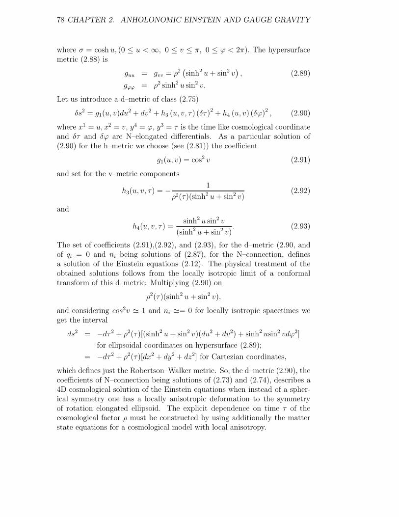
78 CHAPTER 2. ANHOLONOMIC EINSTEIN AND GAUGE GRAVITY
where σ = cosh u, (0 ≤ u < ∞, 0 ≤ v ≤ π, 0 ≤ ϕ < 2π). The hypersurfacemetric (2.88) is
guu = gvv = ρ2(sinh2 u+ sin2 v
), (2.89)
gϕϕ = ρ2 sinh2 u sin2 v.
Let us introduce a d–metric of class (2.75)
δs2 = g1(u, v)du2 + dv2 + h3 (u, v, τ) (δτ)2 + h4 (u, v) (δϕ)2 , (2.90)
where x1 = u, x2 = v, y4 = ϕ, y3 = τ is the time like cosmological coordinateand δτ and δϕ are N–elongated differentials. As a particular solution of(2.90) for the h–metric we choose (see (2.81)) the coefficient
g1(u, v) = cos2 v (2.91)
and set for the v–metric components
h3(u, v, τ) = − 1
ρ2(τ)(sinh2 u+ sin2 v)(2.92)
and
h4(u, v, τ) =sinh2 u sin2 v
(sinh2 u+ sin2 v). (2.93)
The set of coefficients (2.91),(2.92), and (2.93), for the d–metric (2.90, andof qi = 0 and ni being solutions of (2.87), for the N–connection, definesa solution of the Einstein equations (2.12). The physical treatment of theobtained solutions follows from the locally isotropic limit of a conformaltransform of this d–metric: Multiplying (2.90) on
ρ2(τ)(sinh2 u+ sin2 v),
and considering cos2v ' 1 and ni '= 0 for locally isotropic spacetimes weget the interval
ds2 = −dτ 2 + ρ2(τ)[(sinh2 u+ sin2 v)(du2 + dv2) + sinh2 usin2 vdϕ2]
for ellipsoidal coordinates on hypersurface (2.89);
= −dτ 2 + ρ2(τ)[dx2 + dy2 + dz2] for Cartezian coordinates,
which defines just the Robertson–Walker metric. So, the d–metric (2.90), thecoefficients of N–connection being solutions of (2.73) and (2.74), describes a4D cosmological solution of the Einstein equations when instead of a spher-ical symmetry one has a locally anisotropic deformation to the symmetryof rotation elongated ellipsoid. The explicit dependence on time τ of thecosmological factor ρ must be constructed by using additionally the matterstate equations for a cosmological model with local anisotropy.

2.8. ANISOTROPIC COSMOLOGICAL SOLUTIONS 79
Flattened rotation ellipsoid coordinates
In a similar fashion we can construct a locally anisotropic deformation ofthe FRW metric with the symmetry of flattened rotation ellipsoid . Theparametric equation for a such hypersurface is [89]
x2 + y2
1 + σ2+z2
σ2= ρ2,
where σ ≥ 0 and σ = sinh u. The proper for ellipsoid 3D space coordinatesystem is defined
x = ρ cosh u sin v cosϕ, y = ρ cosh u sin v sinϕ
z = ρ sinh u cos v,
where 0 ≤ u <∞, 0 ≤ v ≤ π, 0 ≤ ϕ < 2π. The hypersurface metric is
guu = gvv = ρ2(sinh2 u+ cos2 v
),
gϕϕ = ρ2 sinh2 u cos2 v.
In the rest the cosmological la–solution is described by the same formulas asin the previous subsection but with respect to new canonical coordinates forflattened rotation ellipsoid.
2.8.2 Toroidal FRW universes
Let us construct a cosmological solution of the Einstein equations with toro-idal symmetry. The hypersurface formula of a torus is [89](√
x2 + y2 − ρ c tanhσ)2
+ z2 =ρ2
sinh2 σ.
The 3D space coordinate system is defined
x =ρ sinhα cosϕ
coshα− cos σ, y =
ρ sin σ sinϕ
coshα− cosσ,
z =ρ sinh σ
cosh τ − cosσ,
(−π < σ < π, 0 ≤ α <∞, 0 ≤ ϕ < 2π) .
The hypersurface metric is
gσσ = gαα =ρ2
(coshα− cosσ)2 , gϕϕ =ρ2 sin2 σ
(coshα− cosσ)2 . (2.94)
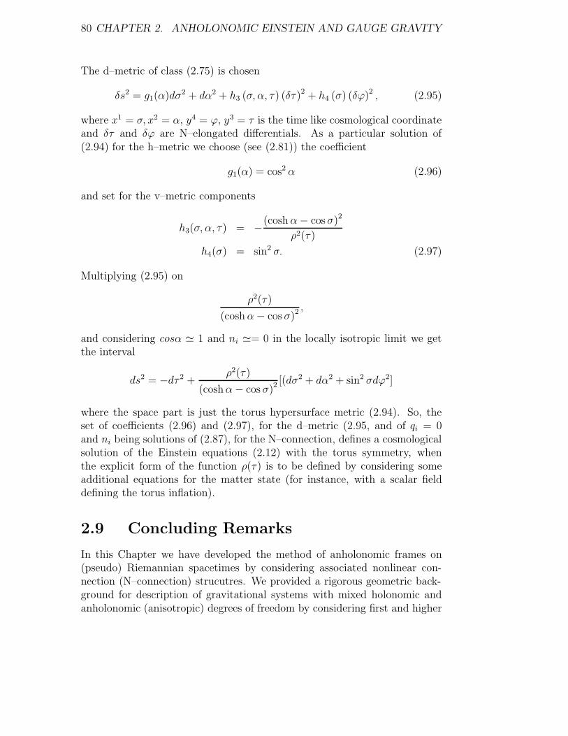
80 CHAPTER 2. ANHOLONOMIC EINSTEIN AND GAUGE GRAVITY
The d–metric of class (2.75) is chosen
δs2 = g1(α)dσ2 + dα2 + h3 (σ, α, τ) (δτ)2 + h4 (σ) (δϕ)2 , (2.95)
where x1 = σ, x2 = α, y4 = ϕ, y3 = τ is the time like cosmological coordinateand δτ and δϕ are N–elongated differentials. As a particular solution of(2.94) for the h–metric we choose (see (2.81)) the coefficient
g1(α) = cos2 α (2.96)
and set for the v–metric components
h3(σ, α, τ) = −(coshα− cosσ)2
ρ2(τ)
h4(σ) = sin2 σ. (2.97)
Multiplying (2.95) on
ρ2(τ)
(coshα− cosσ)2 ,
and considering cosα ' 1 and ni '= 0 in the locally isotropic limit we getthe interval
ds2 = −dτ 2 +ρ2(τ)
(coshα− cos σ)2[(dσ2 + dα2 + sin2 σdϕ2]
where the space part is just the torus hypersurface metric (2.94). So, theset of coefficients (2.96) and (2.97), for the d–metric (2.95, and of qi = 0and ni being solutions of (2.87), for the N–connection, defines a cosmologicalsolution of the Einstein equations (2.12) with the torus symmetry, whenthe explicit form of the function ρ(τ) is to be defined by considering someadditional equations for the matter state (for instance, with a scalar fielddefining the torus inflation).
2.9 Concluding Remarks
In this Chapter we have developed the method of anholonomic frames on(pseudo) Riemannian spacetimes by considering associated nonlinear con-nection (N–connection) strucutres. We provided a rigorous geometric back-ground for description of gravitational systems with mixed holonomic andanholonomic (anisotropic) degrees of freedom by considering first and higher
2.9. CONCLUDING REMARKS 81
order anisotropies induced by anholonomic constraints and correspondingframe bases.
The first key result of this paper is the proof that generic anisotropicstructures of different order are contained in the Einstein theory. We re-formulated the tensor and linear connection formalism for (pseudo) Rieman-nian spaces enables with N–connections and computed the horizonal–verticalsplitting, with respect to anholonomic frames with associated N–connections,of the Einstein equations. The (pseudo) Riemannian spaces enabled withcompatible anholonomic frame and associated N–connection structures andthe metric being a solution of the Einstein equations were called as locallyanisotropic spacetimes (in brief, anisotropic spaces). The next step was thedefinition of gauge field interactions on such spacetimes. We have applied thebundle formalism and extended it to the case of locally anisotropic bases andconsidered a ’pure’ geometric method of deriving the Yang–Mills equationsfor generic locally anisotropic gauge interactions, by genalizing the absolutdifferential calculus and dual forms symmetries for anisotropic spaces.
The second key result was the proof by geometric methods that the Yang–Mills equations for a correspondingly defined Cartan connection in the bun-dle of affine frames on locally anisotropic spacetimes are equivalent to theEinstein equations with anholonomic (N–connection) structures (the originalPopov–Daikhin papers [132, 133] were for the locally isotropic spaces). Theresult was obtained by applying an auxiliary bilinear form on the typical fiberbecause of degeneration of the Killing form for the affine groups. After pro-jection on base spacetimes the dependence on auxiliar values is eliminated.We analyzed also a variant of variational gauge locally anisotropic gauge the-ory by considering a minimal extension of the affine structural group to thede Sitter one, with a nonlinear realization for the gauge group as one wasperformed in a locally isotropic version in Tseytlin’s paper [153]. If someformer our works [186, 172] where devoted to extensions of some models ofgauge gravity to generalized Lagrange and Finsler spaces, in this paper wedemonstrated which manner we could manage with anisotropies arrising inlocally isotropic, but with anholonomic structures, variants of gauge gravity.Here it should be emphasized that anisotropies of different type (Finsler like,or more general ones) could be induced in all variants of gravity theoriesdealing with frame (tetrad, vierbiend, in four dimensions) fields and decom-pisitions of geometrical and physical objects in comonents with respect tosuch frames and associated N–connections. In a similar fashion anisotropiescould arise under nontrivial reductions from higher to lower dimensions inKaluza–Klein theories; in this case the N–connection should be treated asa splitting field modeling the anholonomic (anisotropic) character of somedegrees of freedom.

82 CHAPTER 2. ANHOLONOMIC EINSTEIN AND GAUGE GRAVITY
The third basic result is the construction of a new class of solutions,with generic local anisotropy, of the Einstein equations. For simplicity, wedefined these solutions in the framework of general relativity, but they canbe removed to various variants of gauge and spinor gravity by using corre-sponding decompositions of the metric into the frame fields. We note thatthe obtained class of solutions also holds true for the gauge models of grav-ity which, in this paper, were constructed to b e equivalent to the Einsteintheory. In explicit form we considered the metric ansatz
ds2 = gαβ duαduβ
when gαβ are parametrized by matrices of typeg1 + q1
2h3 + n12h4 q1q2h3 + n1n2h4 q1h3 n1h4
q1q2h3 + n1n2h4 g2 + q22h3 + n2
2h4 q2h3 n2h4
q1h3 q2h3 h3 0n1h4 n2h4 0 h4
(2.98)
with coefficients being some functions of necessary smooth class
gi = gi(xj), qi = qi(x
j , t), ni = ni(xj, t), ha = ha(x
j , t).
Latin indices run respectively i, j, k, ... = 1, 2 and a, b, c, ... = 3, 4 and thelocal coordinates are denoted uα = (xi, y3 = t, y4), where t is treated as atime like coordinate. A metric (2.98) can be diagonalized,
δs2 = gi(xj)(dxi)2
+ ha(xj , t) (δya)2 , (2.99)
with respect to anholonomic frames (2.3) and (2.4), here we write down onlythe ’elongated’ differentials
δt = dz + qi(xj , t)dxi, δy4 = dy4 + ni(x
j , t)dxi.
The ansatz (2.98) was formally introduced in [177] in order to constructlocally anisotropic black hole solutions; in this paper we applied it to cosmo-logical locally anisotropic space–times. In result, we get new metrics whichdescribe locally anisotropic Friedman–Robertson–Walker like universes withthe spherical symmetry deformed to that of rotation (elongated and/or flat-tened) ellipsoid and torus. Such solutions are contained in general relativity:in the simplest diagonal form they are parametrized by distinguished met-rics of type (2.99), given with respect to anholonomic bases, but could bealso described equivalently with respect to a coordinate base by matrices oftype (2.98). The topic of construction of cosmological models with generic

2.9. CONCLUDING REMARKS 83
spacetime and matter field distribution and fluctuation anisotropies is underconsideration.
Now, we point the item of definition of reference frames in gravity the-ories: The form of basic field equations and fundamental laws in generalrelativity do not depend on choosing of coordinate systems and frame bases.Nevertheless, the problem of fixing of an adequate system of reference is also avery important physical task which is not solved by any dynamical equationsbut following some arguments on measuring of physical observables, imposedsymmetry of interactions, types of horizons and singularities, and by takeninto consideration the posed Cauchy problem. Having fixed a class of framevariables, the frame coefficients being presented in the Einstein equations, thetype of constructed solution depends on the chosen holonomic or anholonomicframe structure. As a result one could model various forms of anisotropiesin the framework of the Einsten theory (roughly, on (pseudo) Riemannianspacetimes with corresponding anholonomic frame structures it is possible tomodel Finsler like metrics, or more general ones with anisotropies). Finally, itshould be noted that such questions on stability of obtained solutions, anal-ysis of energy–momentum conditions should be performed in the simplestform with respect to the chosen class of anholonomic frames.

84 CHAPTER 2. ANHOLONOMIC EINSTEIN AND GAUGE GRAVITY

Chapter 3
Anisotropic Taub NUT – DiracSpaces
The aim of this chapter is to outline the theory of gravity on vector bundlesprovided with nonlinear connection structures [108, 109] and to proof thatanholonomic frames with associated nonlinear connection structures can beintroduced in general relativity and in low dimensional and extra dimensionmodels of gravity on (pseudo) Riemannian space–times [177, 179].
3.1 Anholonomic Frames and Nonlinear Con-
nections in General Relativity
The geometry of nonlinear connections on vector and higher order vectorbundles can be reformulated for anholonomic frames given on a (pseudo)Riemannian spacetime of dimension n +m, or n +m1 +m2 + ... +mz, andprovided with a d-metric structure which induces on space–time a canonicald–connection structure (1.49). In this case we can consider a formal splittingof indices with respect to some holonomic and anholonomic frame basis vec-tors. This approach was developed in references [177, 179] with the aim toconstruct exact solutions with generic local anisotropy in general relativityand its low and extra dimension modifications. For simplicity, in the furthersections of this chapter we shall restrict our constructions only to first orderanisotropic structures.
Recently one has proposed a new method of construction of exact solu-tions of the Einstein equations on (pseudo) Riemannian spaces of three, fourand extra dimensions (in brief, 3D, 4D,...), by applying the formalism of an-holonomic moving frames [195]. There were constructed static solutions forblack holes / tori, soliton–dilaton systems and wormhole / flux tube configu-
85

86 CHAPTER 3. ANISOTROPIC TAUB NUT – DIRAC SPACES
rations and for anisotropic generalizations of the Taub NUT metric [194]; allsuch solutions being, in general, with generic local anisotropy. The methodwas elaborated following the geometry of anholonomic frame (super) bundlesand associated nonlinear connections (in brief, N–connection) [180] whichhas a number of applications in generalized Finsler and Lagrange geometry,anholonomic spinor geometry, (super) gravity and strings with anisotropic(anholonomic) frame structures.
In this chapter we restrict our considerations for the 5D Einstein grav-ity. In this case the N–connection coefficients are defined by some partic-ular parametrizations of funfbein, or pentadic, coefficients defining a framestructure on (pseudo) Riemannian spacetime and describing a gravitationaland matter field dynamics with mixed holonomic (unconstrained) and an-holonomic (constrained) variables. We emphasize that the Einstein gravitytheory in arbitrary dimensions can be equivalently formulated with respectto both holonomic (coordinate) and anholonomic frames. In the anholonomiccases the rules of partial and covariant derivation are modified by some pen-tad transforms. The point is to find such values of the anholonomic frame(and associated N–connection) coefficients when the metric is diagonalizedand the Einstein equations are written in a simplified form admitting exactsolutions.
The class of new exact solutions of vacuum Einstein equations describinganisotropic Taub NUT like spacetimes [199] is defined by off–diagonal metricsif they are given with respect to usual coordinate bases. Such metrics can beanholonomically transformed into diagonal ones with coefficients being verysimilar to the coefficients of the isotropic Taub NUT solution but havingadditional dependencies on the 5th coordinate and angular parameters.
We shall use the term locally anisotropic (spacetime) space (in brief,anisotropic space) for a (pseudo) Riemannian space provided with an an-holonomic frame structure induced by a procedure of anholonomic diagonal-ization of a off–diagonal metric.
The Hawking’s [62] suggestion that the Euclidean Taub–NUT metricmight give rise to the gravitational analogue of the Yang–Mills instantonholds true on anisotropic spaces but in this case both the metric and instan-ton have some anisotropically renormalized parameters being of higher di-mension gravitational vacuum polarization origin. The anisotropic EuclideanTaub-NUT metric also satisfies the vacuum Einstein’s equations with zerocosmological constant when the spherical symmetry is deformed, for instance,into ellipsoidal or even toroidal configuration. Such anisotropic Taub-NUTmetrics can be used for generation of deformations of the space part of the lineelement defining an anisotropic modification of the Kaluza-Klein monopolesolutions proposed by Gross and Perry [76] and Sorkin [139].

3.1. N–CONNECTIONS IN GENERAL RELATIVITY 87
In the long-distance limit, neglecting radiation, the relative motion oftwo such anisotropic monopoles can be also described by geodesic motions,like in Ref. [94, 95, 22], but these motions are some anholonomic ones withassociated nonlinear connection structure and effective torsion induced bythe anholonomy of the systems of reference used for modeling anisotropies.The torsion and N–connection corrections vanish if the geometrical objectsare transferred with respect to holonomic (coordinate) frames.
From the mathematical point of view, the new anholonomic geometry ofanisotropic Taub-NUT spaces is also very interesting. In the locally isotropicTaub-NUT geometry there are four Killing-Yano tensors [72]. Three of themform a complex structure realizing the quaternionic algebra and the Taub-NUT manifold is hyper-Kahler. In addition to such three vector-like Killing-Yano tensors, there is a scalar one which exists by virtue of the metric beingof class D, according to Petrov’s classification. Anisotropic deformations ofmetrics to off–diagonal components introduce substantial changes in the ge-ometrical picture. Nevertheless, working with respect to anholonomic frameswith associated nonlinear connection structure the basic properties and re-lations, even being anisotropically modified, are preserved and transformedto similar ones for deformed symmetries [199].
The Schrodinger quantum modes in the Euclidean Taub-NUT geometrywere analyzed using algebraic and analytical methods [72, 73, 58, 48, 71,49, 67]. The Dirac equation was studied in such locally isotropic curvedbackgrounds [57, 88, 23]. One of the aims of this paper is to prove that thisapproach can be developed as to include into consideration anisotropic Taub-NUT backgrounds in the context of the standard relativistic gauge-invarianttheory [203, 34] of the Dirac field.
The purpose of the present work is to develop a general SO(4, 1) gauge-invariant theory of the Dirac fermions [93] which can be considered for locallyanisotropic spaces, for instance, in the external field of the Kaluza-Kleinmonopole [57, 88, 23] which is anisotropically deformed.
Our goal is also to point out new features of the Einstein theory in higherdimension spacetime when the locally anisotropic properties, induced by an-holonomic constraints and extra dimension gravity, are emphasized. Weshall analyze such effects by constructing new classes of exact solutions ofthe Einstein–Dirac equations defining 3D soliton–spinor configurations prop-agating self–consistently in an anisotropic 5D Taub NUT spacetime.
We note that in this paper the 5D spacetime is modeled as a direct timeextension of a 4D Riemannian space provided with a corresponding spinorstructure, i. e. our spinor constructions are not defined by some Clifford al-gebra associated to a 5D bilinear form but, for simplicity, they are consideredto be extended from a spinor geometry defined for a 4D Riemannian space.

88 CHAPTER 3. ANISOTROPIC TAUB NUT – DIRAC SPACES
3.1.1 Anholonomic Einstein–Dirac Equations
In this Section we introduce an ansatz for pseudo Riemannian off–diagonalmetrics and consider the anholonomic transforms diagonalizing such met-rics. The system of field Einstein equations with the spinor matter energy–momentum tensor and of Dirac equations are formulated on 5D pseudo–Riemannian spacetimes constructed as a trivial extension by the time vari-able of a 4D Riemannian space (an anisotropic deformation of the Taub NUTinstanton [199]).
Ansatz for metrics
We consider a 5D pseudo–Riemannian spacetime of signature (+,−,−,−,−), with local coordinates
uα = (xi, ya) = (x0 = t, x1 = r, x2 = θ, y3 = s, y4 = p),
– or more compactly u = (x, y) – where the Greek indices are conventionallysplit into two subsets xi and ya labeled respectively by Latin indices of typei, j, k, ... = 0, 1, 2 and a, b, ... = 3, 4. The 5D (pseduo) Riemannian metric
ds2 = gαβduαduβ (3.1)
is given by a metric ansatz parametrized in the form
gαβ =
1 0 0 0 00 g1 + w 2
1 h3 + n 21 h4 w1w2h3 + n1n2h4 w1h3 n1h4
0 w2w1h3 + n1n2h4 g2 + w 22 h3 + n 2
2 h4 w2h3 n2h4
0 w1h3 w2h3 h3 00 n1h4 n2h4 0 h4
, (3.2)
where the coefficients are some functions of type
g1,2 = g1,2(x1, x2), h3,4 = h3,4(x
1, x2, s), (3.3)
w1,2 = w1,2(x1, x2, s), n1,2 = n1,2(x
1, x2, s).
Both the inverse matrix (metric) as well the metric (3.2) is off–diagonal withrespect to the coordinate basis
∂α ≡∂
duα= (∂i =
∂
dxi, ∂a =
∂
dya) (3.4)
and, its dual basis,
dα ≡ duα = (di = dxi, da = dya). (3.5)

3.1. N–CONNECTIONS IN GENERAL RELATIVITY 89
The metric (3.1) with coefficients (3.2) can be equivalently rewritten inthe diagonal form
δs2 = dt2 + g1 (x) (dx1)2 + g2 (x) (dx2)2 (3.6)
+h3 (x, s) (δy3)2 + h4 (x, s) (δy4)2,
if instead the coordinate bases (3.4) and (3.5) we introduce the anholonomicframes (anisotropic bases)
δα ≡δ
duα= (δi = ∂i −N b
i (u) ∂b, ∂a =∂
dya) (3.7)
and
δα ≡ δuα = (δi = dxi, δa = dya +Nak (u) dxk) (3.8)
where the N–coefficients are parametrized
Na0 = 0, N3
1,2 = w1,2 and N41,2 = n1,2
and define the associated nonlinear connection (N–connection) structure, seedetails in Refs [195, 199, 180].
Einstein equations with anholonomic variables
The metric (3.1) with coefficients (3.2) (equivalently, the d–metric (3.6)) isassumed to solve the 5D Einstein equations
Rαβ −1
2gαβR = κΥαβ, (3.9)
where κ and Υαβ are respectively the coupling constant and the energy–momentum tensor.
The nontrivial components of the Ricci tensor for the metric (3.1) with

90 CHAPTER 3. ANISOTROPIC TAUB NUT – DIRAC SPACES
coefficients (3.2) (equivalently, the d–metric (3.6)) are
R11 = R2
2 = − 1
2g1g2[g••2 −
g•1g•2
2g1− (g•2)
2
2g2+ g
′′1 −
g′1g
′2
2g2− (g
′1)
2
2g1], (3.10)
R33 = R4
4 = − β
2h3h4, (3.11)
R31 = −w1β
2h4− α1
2h4, (3.12)
R32 = −w2β
2h4− α2
2h4,
R41 = − h4
2h3[n∗∗1 + γn∗1] , (3.13)
R42 = − h4
2h3[n∗∗2 + γn∗2] ,
where, for simplicity, the partial derivatives are denoted h• = ∂h/∂x1, f ′ =∂f/∂x2 and f ∗ = ∂f/∂s.
The scalar curvature is computed
R = 2(R1
1 +R33
).
In result of the obtained equalities for some Ricci and Einstein tensorcomponents, we conclude that for the metric ansatz (3.2) the Einstein equa-tions with matter sources are compatible if the coefficients of the energy–momentum d–tensor give with respect to anholonomic bases satisfy the con-ditions
Υ00 = Υ1
1 + Υ33,Υ
11 = Υ2
2 = Υ1,Υ33 = Υ4
4 = Υ3, (3.14)
and could be written in the form
R11 = −κΥ3, (3.15)
R33 = −κΥ1, (3.16)
R3i = κΥ3i, (3.17)
R4i = κΥ4i, (3.18)
where i = 1, 2 and the left parts are given by the components of the Riccitensor (3.10)-(3.13).

3.1. N–CONNECTIONS IN GENERAL RELATIVITY 91
The Einstein equations (3.9), equivalently (3.15)–(3.18), reduce to thissystem of second order partial derivation equations:
g••2 −g•1g
•2
2g1− (g•2)
2
2g2+ g
′′1 −
g′1g
′2
2g2− (g
′1)
2
2g1= −2g1g2Υ3, (3.19)
h∗∗4 −(h∗4)
2
2h4− h∗4h
∗3
2h3= −2h3h4Υ1, (3.20)
βwi + αi = −2h4κΥ3i, (3.21)
n∗∗i + γn∗i = −2h3
h4κΥ4i, (3.22)
where
α1 = h∗4• − h∗4
2
(h•3h3
+h•4h4
), (3.23)
α2 = h∗4′ − h∗4
2
(h′3h3
+h′4h4
), (3.24)
β = h∗∗4 −(h∗4)
2
2h4− h∗4h
∗3
2h3, (3.25)
γ =3
2
h4
h4
∗− h3
h3
∗, (3.26)
and the partial derivatives are denoted, for instance,
g•2 = ∂g2/∂x1 = ∂g2/∂r, g
′1 = ∂g1/∂x
2 = ∂g1/θ,
h∗3 = ∂h3/∂s = ∂h3/∂ϕ (or ∂h3/∂y4, for s = y4).
Dirac equations in anisotropic space–times
The problem of definition of spinors in locally anisotropic spaces and in spaceswith higher order anisotropy was solved in Refs. [180]. In this paper weconsider locally anisotropic Dirac spinors given with respect to anholonomicframes with associated N–connection structure on a 5D (pseudo) Riemannianspace V (1,2,2) constructed by a direct time extension of a 4D Riemannianspace with two holonomic and two anholonomic variables.
Having an anisotropic d–metric
gαβ(u) = (gij(u), hab(u)) = (1, gi(u), ha(u)),
i = 1, 2; i = 0, 1, 2; a = 3, 4,
defined with respect to an anholonomic basis (1.16) we can easily define thefunfbein (pentad) fields
fµ = fµµ δµ = fi = f i
i δi, fa = faa∂a, (3.27)
fµ = fµµ δ
µ = f i = fiid
i, , fa = faa δ
a

92 CHAPTER 3. ANISOTROPIC TAUB NUT – DIRAC SPACES
satisfying the conditions
gij = fii f
j
j gij and hab = faa f
bbhab,
gij = diag[1,−1− 1] and hab = diag[−1,−1].
For a diagonal d-metric of type (1.39) we have
f ii =
√|gi|δi
i and faa =
√|ha|δa
a,
where δii and δa
a are Kronecker’s symbols.We can also introduce the corresponding funfbiends which are related
with the off–diagonal metric ansatz (3.2) for gαβ,
eµ = eµµ∂µ and eµ = e
µµ∂
µ (3.28)
satisfying the conditions
gαβ = eααe
β
βgαβ for gαβ = diag[1,−1,−1,−1,−1],
eααe
µα = δµ
α and eααe
αµ = δα
µ .
The Dirac spinor fields on locally anisotropic deformations of Taub NUTspaces,
Ψ (u) = [Ψα (u)] = [ψI (u) , χI (u)],
where I = 0, 1, are defined with respect to the 4D Euclidean tangent subspacebelonging the tangent space to V (1,2,2). The 4×4 dimensional gamma matricesγα′ = [γ1′ , γ2′, γ3′ , γ4′] are defined as to satisfy the relation
γα′ , γβ′
= 2gα′β′ , (3.29)
whereγα′ γβ′
is a symmetric commutator, gα′β′ = (−1,−1,−1,−1), which
generates a Clifford algebra distinguished on two holonomic and two anholo-nomic directions (hereafter the primed indices will run values on the Eu-clidean and/or Riemannian, 4D component of the 5D pseudo–Riemannianspacetime). In order to extend the (3.29) relations for unprimed indicesα, β... we conventionally complete the set of primed gamma matrices with amatrix γ0, i. .e. write γα = [γ0, γ1, γ2, γ3, γ4] when
γα, γβ
= 2gαβ.

3.1. N–CONNECTIONS IN GENERAL RELATIVITY 93
The coefficients of gamma matrices can be computed with respect tocoordinate bases (1.2) or with respect to anholonomic bases (1.16) by usingrespectively the funfbein coefficients (3.27) and (3.28),
γα(u) = eαα(u)γα and γβ(u) = fβ
β (u)γβ,
were by γα(u) we denote the curved spacetime gamma matrices and by γβ(u)we denote the gamma matrices adapted to the N–connection structure.
The covariant derivation of Dirac spinor field Ψ (u) , 5αΨ, can be definedwith respect to a pentad decomposition of the off–diagonal metric (3.2)
5αΨ =
[∂α +
1
4Cαβγ (u) eα
α (u) γβγγ
]Ψ, (3.30)
where the coefficients
Cαβγ (u) =(Dγe
αα
)eβαe
γγ
are called the rotation Ricci coefficients; the covariant derivativeDγ is definedby the usual Christoffel symbols for the off–diagonal metric.
We can also define an equivalent covariant derivation of the Dirac spinorfield,
−→5αΨ, by using pentad decompositions of the diagonalized d–metric(1.39),
−→5αΨ =
[δα +
1
4C
[δ]αβγ (u) fα
α (u) γβγγ
]Ψ, (3.31)
where there are introduced N–elongated partial derivatives and the coeffi-cients
C[δ]αβγ (u) =
(D[δ]
γ fαα
)fβαf
γγ
are transformed into rotation Ricci d–coefficients which together with thed–covariant derivative D
[δ]γ are defined by anholonomic pentads and anholo-
nomic transforms of the Christoffel symbols.For diagonal d–metrics the funfbein coefficients can be taken in their turn
in diagonal form and the corresponding gamma matrix γα (u) for anisotropiccurved spaces are proportional to the usual gamma matrix in flat spacesγγ . The Dirac equations for locally anisotropic spacetimes are written in thesimplest form with respect to anholonomic frames,
(iγα (u)−→5α − µ)Ψ = 0, (3.32)

94 CHAPTER 3. ANISOTROPIC TAUB NUT – DIRAC SPACES
where µ is the mass constant of the Dirac field. The Dirac equations are theEuler equations for the Lagrangian
L(1/2) (u) =√|g|[Ψ+ (u) γα (u)
−→5αΨ (u) (3.33)
−(−→5αΨ+ (u))γα (u)Ψ (u)]− µΨ+ (u)Ψ (u),
where by Ψ+ (u) we denote the complex conjugation and transposition of thecolumn Ψ (u) .
Varying L(1/2) on d–metric (3.33) we obtain the symmetric energy–mo-mentum d–tensor
Υαβ (u) =i
4[Ψ+ (u) γα (u)
−→5βΨ (u) + Ψ+ (u) γβ (u)−→5αΨ (u)
−(−→5αΨ+ (u))γβ (u)Ψ (u)− (
−→5βΨ+ (u))γα (u)Ψ (u)].(3.34)
We choose such spinor field configurations in curved spacetime as to be sat-isfied the conditions (3.14).
One can introduce similar formulas to (3.32)–(3.34) for spacetimes pro-vided with off-diagonal metrics with respect to holonomic frames by changingof operators γα (u)→ γα (u) and
−→5β →5β.
3.1.2 Anisotropic Taub NUT – Dirac Spinor Solutions
By straightforward calculations we can verify that because the conditionsD
[δ]γ fα
α = 0 are satisfied the Ricci rotation coefficients vanishes,
C[δ]αβγ (u) = 0 and
−→5αΨ = δαΨ,
and the anisotropic Dirac equations (3.32) transform into
(iγα (u) δα − µ)Ψ = 0. (3.35)
Further simplifications are possible for Dirac fields depending only oncoordinates (t, x1 = r, x2 = θ), i. e. Ψ = Ψ(xk) when the equation (3.35)transforms into
(iγ0∂t + iγ1 1√|g1|
∂1 + iγ2 1√|g2|
∂2 − µ)Ψ = 0.
The equation (3.35) simplifies substantially in ζ–coordinates(t, ζ1 = ζ1(r, θ), ζ2 = ζ2(r, θ)
),

3.1. N–CONNECTIONS IN GENERAL RELATIVITY 95
defined as to be satisfied the conditions
∂
∂ζ1=
1√|g1|
∂1 and∂
∂ζ2=
1√|g2|
∂2 (3.36)
We get
(−iγ0∂
∂t+ iγ1
∂
∂ζ1+ iγ2
∂
∂ζ2− µ)Ψ(t, ζ1, ζ2) = 0. (3.37)
The equation (3.37) describes the wave function of a Dirac particle of mass µpropagating in a three dimensional Minkowski flat plane which is imbeddedas an anisotropic distribution into a 5D pseudo–Riemannian spacetime.
The solution Ψ = Ψ(t, ζ1, ζ2) of (3.37) can be written
Ψ =
Ψ(+)(ζ) = exp [−i(k0t+ k1ζ
1 + k2ζ2)]ϕ0(k)
for positive energy;Ψ(−)(ζ) = exp [i(k0t+ k1ζ
1 + k2ζ2)]χ0(k)
for negative energy,
with the condition that k0 is identified with the positive energy and ϕ0(k)and χ0(k) are constant bispinors. To satisfy the Klein–Gordon equation wemust have
k2 = k20 − k2
1 − k22 = µ2.
The Dirac equations implies
(σiki − µ)ϕ0(k) and (σiki + µ)χ0(k),
where σi(i = 0, 1, 2) are Pauli matrices corresponding to a realization ofgamma matrices as to a form of splitting to usual Pauli equations for thebispinors ϕ0(k) and χ0(k).
In the rest frame for the horizontal plane parametrized by coordinatesζ = t, ζ1, ζ2 there are four independent solutions of the Dirac equations,
ϕ0(1)(µ, 0) =
1000
, ϕ0(2)(µ, 0) =
0100
,
χ0(1)(µ, 0) =
0010
, χ0(2)(µ, 0) =
0001
.

96 CHAPTER 3. ANISOTROPIC TAUB NUT – DIRAC SPACES
In order to satisfy the conditions (3.14) for compatibility of the equations(3.19)–(3.22) we must consider wave packets of type (for simplicity, we canuse only superpositions of positive energy solutions)
Ψ(+)(ζ) =
∫d3p
2π3
µ√µ2 + (k2)2
×∑
[α]=1,2,3
b(p, [α])ϕ[α](k) exp [−ikiζi] (3.38)
when the coefficients b(p, [α]) define a current (the group velocity)
J2 =∑
[α]=1,2,3
∫d3p
2π3
µ√µ2 + (k2)2
|b(p, [α])|2 p2√µ2 + (k2)2
≡< p2√µ2 + (k2)2
>
with |p2| ∼ µ and the energy–momentum d–tensor (3.34) has the next non-trivial coefficients
Υ00 = 2Υ(ζ1, ζ2) = k0Ψ
+γ0Ψ,
Υ11 = −k1Ψ
+γ1Ψ,Υ22 = −k2Ψ
+γ2Ψ (3.39)
where the holonomic coordinates can be reexpressed ζ i = ζ i(xi). We musttake two or more waves in the packet and choose such coefficients b(p, [α]),satisfying corresponding algebraic equations, as to have in (3.39) the equali-ties
Υ11 = Υ2
2 = Υ(ζ1, ζ2) = Υ(x1, x2), (3.40)
required by the conditions (3.34).
3.2 Taub NUT Solutions with Generic Local
Anisotropy
The Kaluza-Klein monopole [76, 139] was obtained by embedding the Taub-NUT gravitational instanton into five-dimensional theory, adding the timecoordinate in a trivial way. There are anisotropic variants of such solutions[199] when anisotropies are modelled by effective polarizations of the inducedmagnetic field. The aim of this Section is to analyze such Taub–NUT solu-tions for both cases of locally isotropic and locally anisotropic configurations.
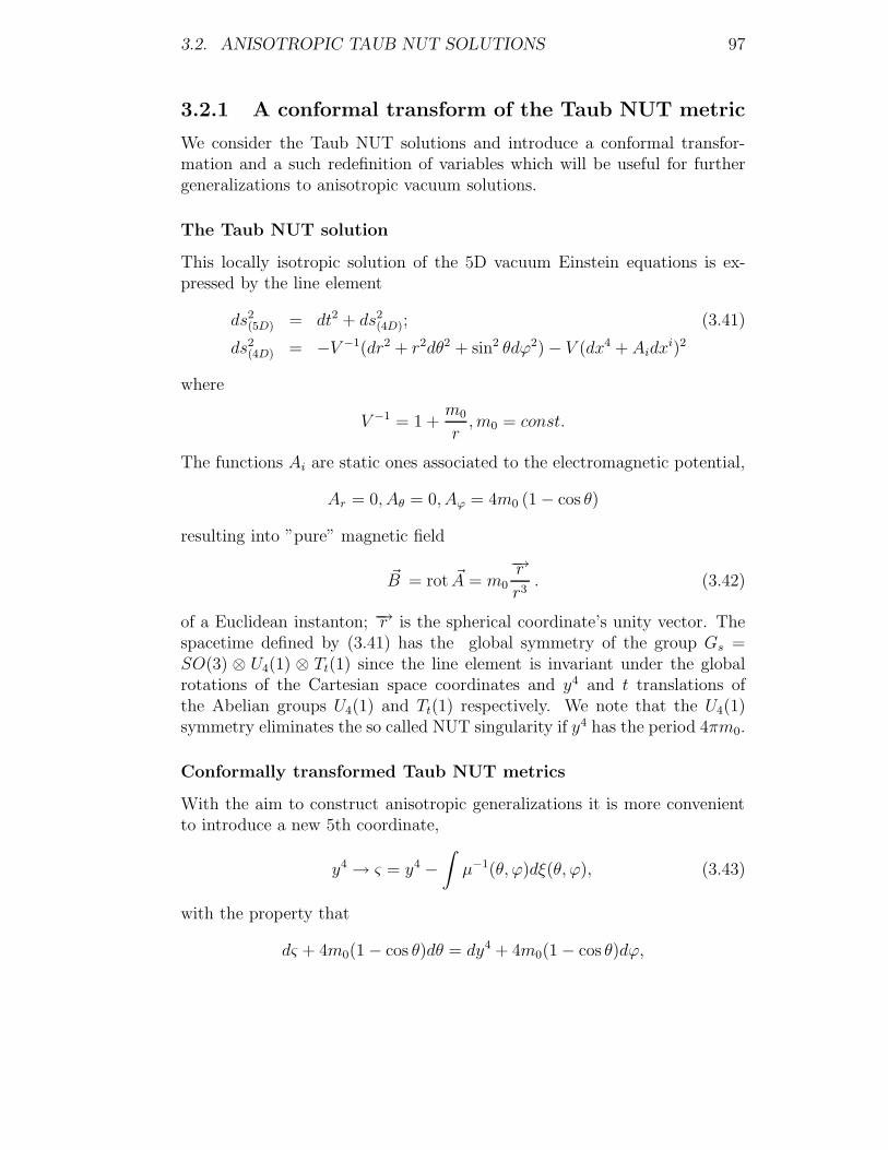
3.2. ANISOTROPIC TAUB NUT SOLUTIONS 97
3.2.1 A conformal transform of the Taub NUT metric
We consider the Taub NUT solutions and introduce a conformal transfor-mation and a such redefinition of variables which will be useful for furthergeneralizations to anisotropic vacuum solutions.
The Taub NUT solution
This locally isotropic solution of the 5D vacuum Einstein equations is ex-pressed by the line element
ds2(5D) = dt2 + ds2
(4D); (3.41)
ds2(4D) = −V −1(dr2 + r2dθ2 + sin2 θdϕ2)− V (dx4 + Aidx
i)2
where
V −1 = 1 +m0
r,m0 = const.
The functions Ai are static ones associated to the electromagnetic potential,
Ar = 0, Aθ = 0, Aϕ = 4m0 (1− cos θ)
resulting into ”pure” magnetic field
~B = rot ~A = m0
−→rr3. (3.42)
of a Euclidean instanton; −→r is the spherical coordinate’s unity vector. Thespacetime defined by (3.41) has the global symmetry of the group Gs =SO(3) ⊗ U4(1) ⊗ Tt(1) since the line element is invariant under the globalrotations of the Cartesian space coordinates and y4 and t translations ofthe Abelian groups U4(1) and Tt(1) respectively. We note that the U4(1)symmetry eliminates the so called NUT singularity if y4 has the period 4πm0.
Conformally transformed Taub NUT metrics
With the aim to construct anisotropic generalizations it is more convenientto introduce a new 5th coordinate,
y4 → ς = y4 −∫µ−1(θ, ϕ)dξ(θ, ϕ), (3.43)
with the property that
dς + 4m0(1− cos θ)dθ = dy4 + 4m0(1− cos θ)dϕ,

98 CHAPTER 3. ANISOTROPIC TAUB NUT – DIRAC SPACES
which holds for
dξ = µ(θ, ϕ)d(ς − y4) =∂ξ
∂θdθ +
∂ξ
∂ϕdϕ,
when
∂ξ
∂θ= 4m0(1− cos θ)µ,
∂ξ
∂ϕ= −4m0(1− cos θ)µ,
and, for instance,
µ = (1− cos θ)−2 exp[θ − ϕ].
The changing of coordinate (3.43) describe a re–orientation of the 5th coor-dinate in a such way as we could have only one nonvanishing component ofthe electromagnetic potential
Aθ = 4m0 (1− cos θ) .
The next step is to perform a conformal transform,
ds2(4D) → ds2
(4D) = V ds2(4D)
and to consider the 5D metric
ds2(5D) = dt2 + ds2
(4D); (3.44)
ds2(4D) = −(dr2 + r2dθ2)− r2 sin2 θdϕ2 − V 2(dζ + Aθdθ)
2,
(not being an exact solution of the Einstein equations) which will transforminto some exact solutions after corresponding anholonomic transforms.
Here, we emphasize that we chose the variant of transformation of a lo-cally isotropic non–Einsteinian metrics into an anisotropic one solving thevacuum Einstein equations in order to illustrate a more simple procedureof construction of 5D vacuum metrics with generic local anisotropy. As ametter of principle we could remove vacuum isotropic solutions into vacuumanisotropic ones, but the formula in this case would became very comber-some.. The fact of selection as an isotropic 4D Riemannian background justthe metric from the linear interval ds2
(4D) can be treated as a conformal trans-formation of an instanton solution which is anisotropically deformed and puttrivially (by extension to the time like coordinate) into a 5D metric as togenerate a locally isotropic vacuum gravitational field.

3.2. ANISOTROPIC TAUB NUT SOLUTIONS 99
3.2.2 Anisotropic Taub NUT solutions with magnetic
polarization
We outline two classes of exact solutions of 5D vacuum Einstein equationswith generic anisotropies (see details in Ref. [199]) which will be extendedto configurations with spinor matter field source.
Solutions with angular polarization
The ansatz for a d–metric (1.39), with a distinguished anisotropic dependenceon the angular coordinate ϕ, when s = ϕ, is taken in the form
δs2 = dt2 − δs2(4D),
δs2(4D) = −(dr2 + r2dθ2)− r2 sin2 θdϕ2 − V 2(r)η2
4(θ, ϕ)δς2,
δς = dς + n2(θ, ϕ)dθ,
where the values η24(θ, ϕ) (we use non–negative values η2
4 not changing thesignature of metrics) and n2(θ, ϕ) must be found as to satisfy the vacuumEinstein equations in the form (3.19)–(3.22). We can verify that the data
x0 = t, x1 = r, x2 = θ, y3 = s = ϕ, y4 = ς, (3.45)
g0 = 1, g1 = −1, g2 = −r2, h3 = −r2 sin2 θ,
h4 = V 2 (r) η2(ϕ), η
2(ϕ) = [1 +$(r, θ)ϕ]2, wi = 0;
n0,1 = 0;n2 = n2[0] (r, θ) + n2[1] (r, θ) /[1 +$(r, θ)ϕ]2.
give an exact solution. If we impose the condition to obtain in the locallyisotropic limit just the metric (3.44), we have to choose the arbitrary func-tions from the general solution of (3.20) as to have
η2(ϕ) = [1 +$(r, θ)ϕ]2 → 1 for $(r, θ)ϕ→ 0.
For simplicity, we can analyze only angular anisotropies with $ = $(θ),when
η2(ϕ) = η2
(ϕ)(θ, ϕ) = [1 +$(θ)ϕ]2.
In the locally isotropic limit of the solution for n2 (r, θ, ϕ), when $ϕ→ 0,we could obtain the particular magnetic configuration contained in the metric(3.44) if we impose the condition that
n2[0] (r, θ) + n2[1] (r, θ) = Aθ = 4m0 (1− cos θ) ,

100 CHAPTER 3. ANISOTROPIC TAUB NUT – DIRAC SPACES
which defines only one function from two unknown values n2[0] (r, θ) andn2[1] (r, θ) . This could have a corresponding physical motivation. From theusual Kaluza–Klein procedure we induce the 4D gravitational field (met-ric) and 4D electro–magnetic field (potentials Ai), which satisfy the Maxwellequations in 4D pseudo–Riemannian space–time. For the case of spherical, lo-cally isotropic, symmetries the Maxwell equations can be written for vacuummagnetic fields without any polarizations. When we introduce into considera-tion anholonomic constraints and locally anisotropic gravitational configura-tions the effective magnetic field could be effectively renormalized by higherdimension gravitational field. This effect, for some classes of anisotropies,can be modeled by considering that the constant m0 is polarized,
m0 → m (r, θ, ϕ) = m0ηm (r, θ, ϕ)
for the electro–magnetic potential and resulting magnetic field. For ”pure”angular anisotropies we write that
n2 (θ, ϕ) = n2[0] (θ) + n2[1] (θ) /[1 +$(θ)ϕ]2
= 4m0ηm (θ, ϕ) (1− cos θ) ,
for
η2(ϕ) (θ, ϕ) = η2
(ϕ)[0] (θ) + η2(ϕ)[1] (θ) /[1 +$(θ)ϕ]2.
This could result in a constant angular renormalization even $(θ)ϕ→ 0.
Solutions with extra–dimension induced polarization
Another class of solutions is constructed if we consider a d–metric of the type(1.39), when s = ς, with anisotropic dependence on the 5th coordinate ς,
δs2 = dt2 − δs2(4D),
δs2(4D) = −(dr2 + r2dθ2)− r2 sin2 θdϕ2 − V 2(r)η2
(ς)(θ, ς)δς2,
δς = dς + w3(θ, ς)dθ,
where, for simplicity, we omit possible anisotropies on variable r, i. e. westate that η(ς) and w2 are not functions on r.
The data for a such solution are
x0 = t, x1 = r, x2 = θ, y3 = s = ς, y4 = ϕ, (3.46)
g0 = 1, g1 = −1, g2 = −r2, h4 = −r2 sin2 θ,
h3 = V 2 (r) η2(ς), η
2(ς) = η2
(ς)(r, θ, ς), n0,1 = 0;
w0,1 = 0, w2 = 4m0ηm (θ, ς) (1− cos θ) , n0 = 0,
n1,2 = n1,2[0] (r, θ) + n1,2[1] (r, θ)
∫η−3
(ς) (r, θ, ς)dς,

3.3. ANISOTROPIC TAUB NUT–DIRAC FIELDS 101
where the function η(ς) = η(ς)(r, θ, ς) is an arbitrary one as follow for the caseh∗4 = 0, for angular polarizations we state, for simplicity, that η(ς) does notdepend on r, i. e. η(ς) = η(ς)(θ, ς). We chose the coefficient
w4 = 4m0ηm (θ, ς) (1− cos θ)
as to have compatibility with the locally isotropic limit when w2 ' Aθ witha ”polarization” effect modeled by ηm (θ, ς) , which could have a constantcomponent ηm ' ηm[0] = const for small anisotropies. In the simplest caseswe can fix the conditions n1,2[0,1] (r, θ) = 0. All functions η2
(ς), ηm and n1,2[0,1]
can be treated as some possible induced higher dimensional polarizations.
3.3 Anisotropic Taub NUT–Dirac Fields
In this Section we construct two new classes of solutions of the 5D Einstein–Dirac fields in a manner as to extend the locally anisotropic Taub NUTmetrics defined by data (3.45) and (3.46) as to be solutions of the Einsteinequations (3.19)–(3.22) with a nonvanishing diagonal energy momentum d–tensor
Υαβ = 2Υ(r, θ),Υ(r, θ),Υ(r, θ), 0, 0
for a Dirac wave packet satisfying the conditions (3.39) and (3.40).
3.3.1 Dirac fields and angular polarizations
In order to generate from the data (3.45) a new solution with Dirac spinormatter field we consider instead of a linear dependence of polarization,
η(ϕ) ∼ [1 +$ (r, θ)ϕ],
an arbitrary function η(ϕ) (r, θ, ϕ) for which
h4 = V 2(r)η2(ϕ) (r, θ, ϕ)
is an exact solution of the equation (3.20) with Υ1 = Υ (r, θ) . With respectto the variable η2
(ϕ) (r, θ, ϕ) this component of the Einstein equations becomeslinear
η∗∗(ϕ) + r2 sin2 θΥη(ϕ) = 0 (3.47)
which is a second order linear differential equation on variable ϕ with para-metric dependencies of the coefficient r2 sin2 θΥ on coordinates (r, θ) . The

102 CHAPTER 3. ANISOTROPIC TAUB NUT – DIRAC SPACES
solution of equation (3.47) is to be found following the method outlined inRef. [82]:
η(ϕ) = C1 (r, θ) cosh[ϕr sin θ√|Υ (r, θ)|+ C2 (r, θ)],
Υ (r, θ) < 0; (3.48)
= C1 (r, θ) + C2 (r, θ)ϕ,Υ (r, θ) = 0; (3.49)
= C1 (r, θ) cos[ϕr sin θ√
Υ (r, θ) + C2 (r, θ)],
Υ (r, θ) > 0, (3.50)
where C1,2 (r, θ) are some functions to be defined from some boundary con-ditions. The first solution (3.48), for negative densities of energy should beexcluded as unphysical, the second solution (3.49) is just that from (3.45)for the vacuum case. A new interesting physical situation is described bythe solution (3.50) when we obtain a Taub NUT anisotropic metric with pe-riodic anisotropic dependencies on the angle ϕ where the periodicity couldvariate on coordinates (r, θ) as it is defined by the energy density Υ (r, θ) . Forsimplicity, we can consider a package of spinor waves with constant value ofΥ = Υ0 and fix some boundary and coordinate conditions when C1,2 = C1,2[0]
are constant. This type of anisotropic Taub NUT solutions are described bya d–metric coefficient
h4 = V 2(r)C21[0] cos2[ϕr sin θ
√Υ0 + C2[0]]. (3.51)
Putting this value into the formulas (3.23), (3.24) and (3.25) for coefficientsin equations (3.21) we can express α1,2 = α1,2[h3, h4,Υ0] and β = β[h3, h4,Υ0](we omit these rather simple but cumbersome formulas) and in consequencewe can define the values w1,2 by solving linear algebraic equations:
w1,2 (r, θ, ϕ) = α1,2 (r, θ, ϕ) /β (r, θ, ϕ) .
Having defined the values (3.51) it is a simple task of two integrations onϕ in order to define
n2 = n2[0] (r, θ)
[ln
1 + cos κ
1− cos κ+
1
1− cos κ+
1
1− sin κ
]+n2[1] (r, θ) , (3.52)
were
κ = ϕr sin θ√
Υ0 + C2[0],
n2[0,1] (r, θ) are some arbitrary functions to be defined by boundary condi-tions. We put n0,1 = 0 to obtain in the vacuum limit the solution (3.45).

3.3. ANISOTROPIC TAUB NUT–DIRAC FIELDS 103
Finally, we can summarize the data defining an exact solution for ananisotropic (on angle ϕ) Dirac wave packet – Taub NUT configuration:
x0 = t, x1 = r, x2 = θ, y3 = s = ϕ, y4 = ς, (3.53)
g0 = 1, g1 = −1, g2 = −r2, h3 = −r2 sin2 θ,
h4 = V 2 (r) η2(ϕ), η(ϕ) = C1 (r, θ) cos κ(r, θ, ϕ),
wi = 0, n0,1 = 0, n2 = n2 (r, θ, κ(r, θ, ϕ)) see (3.52),
Ψ = Ψ(+)(ζ1,2(x1, x2)
)see (3.38),
Υ = Υ(ζ1,2(x1, x2)
)see (3.39).
This solution will be extended to additional soliton anisotropic configurationsin the next Section.
3.3.2 Dirac fields and extra dimension polarizations
Now we consider a generalization of the data (3.46) for generation of a newsolution, with generic local anisotropy on extra dimension 5th coordinate, ofthe Einstein – Dirac equations. Following the equation (3.21) we concludethat there are not nonvacuum solutions of the Einstein equations (with Υ 6=0) if h∗4 = 0 which impose the condition Υ = 0 for h3, h4 6= 0. So, we have toconsider that the d–metric component h4 = −r2 sin2 θ from the data (3.46)is generalized to a function h4 (r, θ, ς) satisfying a second order nonlineardifferential equation on variable ς with coefficients depending parametricallyon coordinates (r, θ) . The equation (i. e. (3.21)) can be linearized (see Ref.[82]) if we introduce a new variable h4 = h2,
h∗∗ − h∗32h3
h∗ + h3Υh = 0,
which, in its turn, can be transformed :a) to a Riccati form if we introduce a new variable v, for which h = v∗/v,
v∗ + v2 − h∗32h3
v + h3Υ = 0; (3.54)
b) to the so–called normal form [82],
λ∗∗ + Iλ = 0, (3.55)
obtained by a redefinition of variables like
λ = h exp
[−1
4
∫h∗3h3dς
]= h h
−1/43

104 CHAPTER 3. ANISOTROPIC TAUB NUT – DIRAC SPACES
where
I = h3Υ−1
16
h∗3h3
+1
4
(h∗3h3
)∗.
We can construct explicit series and/or numeric solutions (for instance, byusing Mathematica or Maple programs) of both type of equations (3.54)and normal (3.55) for some stated boundary conditions and type of polar-ization of the coefficient h3 (r, θ, ς) = V 2 (r) η2
(ς)(r, θ, ς) and, in consequence,
to construct different classes of solutions for h4 (r, θ, ς) . In order to havecompatibility with the data (3.46) we must take h4 in the form
h4 (r, θ, ς) = −r2 sin2 θ + h4(ς) (r, θ, ς) ,
where h4(ς) (r, θ, ς) vanishes for Υ→ 0.Having defined a value of h4 (r, θ, ς) we can compute the coefficients (3.23),
(3.24) and (3.25) and find from the equations (3.21)
w1,2 (r, θ, ς) = α1,2 (r, θ, ς) /β (r, θ, ς) .
From the equations (3.22), after two integrations on variable ς one obtainsthe values of n1,2 (r, θ, ς) . Two integrations of equations (3.22) define
ni(r, θ, ς) = ni[0](r, θ)
∫ ς
0
dz
∫ z
0
dsP (r, θ, s) + ni[1](r, θ),
where
P ≡ 1
2(h∗3h3− 3
h∗4h4
)
and the functions ni[0](r, θ) and ni[1](r, θ) on (r, θ) have to be defined by solv-ing the Cauchy problem. The boundary conditions of both type of coefficientsw1,2 and n1,2 should be expressed in some forms transforming into correspond-ing values for the data (3.46) if the source Υ→ 0. We omit explicit formulasfor exact Einstein–Dirac solutions with ς–polarizations because their formsdepend very strongly on the type of polarizations and vacuum solutions.
3.4 Anholonomic Dirac–Taub NUT Solitons
In the next subsections we analyze two explicit examples when the spinor fieldinduces two dimensional, depending on three variables, solitonic anisotropies.

3.4. ANHOLONOMIC DIRAC–TAUB NUT SOLITONS 105
3.4.1 Kadomtsev–Petviashvili type solitons
By straightforward verification we conclude that the d–metric componenth4(r, θ, s) could be a solution of Kadomtsev–Petviashvili (KdP) equation [81](the first methods of integration of 2+1 dimensional soliton equations wheredeveloped by Dryuma [55] and Zakharov and Shabat [212])
h∗∗4 + ε(h4 + 6h4h
′4 + h′′′4
)′= 0, ε = ±1, (3.56)
if the component h3(r, θ, s) satisfies the Bernoulli equations [82]
h∗3 + Y (r, θ, s) (h3)2 + Fε (r, θ, s)h3 = 0, (3.57)
where, for h∗4 6= 0,
Y (r, θ, s) = κΥh4
h∗4, (3.58)
and
Fε (r, θ, s) =h∗4h4
+2ε
h∗4
(h4 + 6h4h
′4 + h′′′4
)′.
The three dimensional integral variety of (3.57) is defined by formulas
h−13 (r, θ, s) = h−1
3(x) (r, θ)Eε
(xi, s
)×∫
Y (r, θ, s)
Eε (r, θ, s)ds,
where
Eε (r, θ, s) = exp
∫Fε (r, θ, s) ds
and h3(x) (r, θ) is a nonvanishing function.In the vacuum case Y (r, θ, s) = 0 and we can write the integral variety
of (3.57)
h(vac)3 (r, θ, s) = h
(vac)3(x) (r, θ) exp
[−∫Fε (r, θ, s) ds
].
We conclude that a solution of KdP equation (3.57) could be generatedby a non–perturbative component h4(r, θ, s) of a diagonal h–metric if thesecond component h3 (r, θ, s) is a solution of Bernoulli equations (3.57) withcoefficients determined both by h4 and its partial derivatives and by the Υ1
1
component of the energy–momentum d–tensor (see (3.40)). The parameters(coefficients) of (2+1) dimensional KdV solitons are induced by gravity andspinor constants and spinor field configuration defining locally anisotropicinteractions of packets of Dirac’s spinor waves.

106 CHAPTER 3. ANISOTROPIC TAUB NUT – DIRAC SPACES
3.4.2 (2+1) sine–Gordon type solitons
In a similar manner we can prove that solutions h4(r, θ, s) of (2+1) sine–Gordon equation (see, for instance, [61, 90, 207])
h∗∗4 + h′′4 − h4 = sin(h4)
also induce solutions for h3 (r, θ, s) following from the Bernoulli equation
h∗3 + κE(r, θ)h4
h∗4(h3)
2 + F (r, θ, s) h3 = 0, h∗4 6= 0,
where
F (r, θ, s) =h∗4h4
+2
h∗4
[h′′4 − h4 − sin(h4)
].
The general solutions (with energy–momentum sources and in vacuum cases)are constructed by a corresponding redefinition of coefficients in the formu-las from the previous subsection. We note that we can consider both typeof anisotropic solitonic polarizations, depending on angular variable ϕ oron extra dimension coordinate ς. Such classes of solutions of the Einstein–Dirac equations describe three dimensional spinor wave packets induced andmoving self–consistently on solitonic gravitational locally anisotropic configu-rations. In a similar manner, we can consider Dirac wave packets generatingand propagating on locally anisotropic black hole (with rotation ellipsoidhorizons), black tori, anisotropic disk and two or three dimensional blackhole anisotropic gravitational structures [195]. Finally, we note that suchgravitational solitons are induced by Dirac field matter sources and are dif-ferent from those soliton solutions of vacuum Einstein equations originallyconsidered by Belinski and Zakharov [31].
Finally, we conclude that we have argued that the anholonomic framemethod can be applied for construction on new classes of Einstein–Diracequations in five dimensional (5D) space–times. Subject to a form of metricansatz with dependencies of coefficients on two holonomic and one anholo-nomic variables we obtained a very simplified form of field equations whichadmit exact solutions. We have identified two classes of solutions describingTaub NUT like metrics with anisotropic dependencies on angular parameteror on the fifth coordinate. We have shown that both classes of anisotropicvacuum solutions can be generalized to matter sources with the energy–momentum tensor defined by some wave packets of Dirac fields. Althoughthe Dirac equation is a quantum one, in the quasi–classical approximation wecan consider such spinor fields as some spinor waves propagating in a three

3.4. ANHOLONOMIC DIRAC–TAUB NUT SOLITONS 107
dimensional Minkowski plane which is imbedded in a self–consistent mannerin a Taub–NUT anisotropic space–time. At the classical level it should beemphasized that the results of this paper are very general in nature, depend-ing in a crucial way only on the locally Lorentzian nature of 5D space–timeand on the supposition that this space–time is constructed as a trivial timeextension of 4D space–times. We have proved that the new classes of so-lutions admit generalizations to nontrivial topological configurations of 3Ddimensional solitons (induced by anisotropic spinor matter) defined as solu-tions Kadomtsev–Petviashvili or sine–Gordon equations.

108 CHAPTER 3. ANISOTROPIC TAUB NUT – DIRAC SPACES

Part II
Anisotropic Spinors
109


111
Spinor variables and interactions of spinor fields on Finsler spaces wereused in a heuristic manner, for instance, in works [19, 124], where the problemof a rigorous definition of spinors for locally anisotropic spaces was not con-sidered. Here we note that, in general, the nontrivial nonlinear connectionand torsion structures and possible incompatibility of metric and connec-tions makes the solution of the mentioned problem very sophisticate. Thegeometric definition of locally anisotropic spinors and a detailed study of therelationship between Clifford, spinor and nonlinear and distinguished connec-tions structures in vector bundles, generalized Lagrange and Finsler spacesare presented in Refs. [163, 162, 165].
The purpose of this Part is to summarize our investigations [163, 162,165, 186, 169] on formulation of the theory of classical and quantum fieldinteractions on locally anisotropic spaces. We receive primary attention tothe development of the necessary geometric framework: to propose an ab-stract spinor formalism and formulate the differential geometry of locallyanisotropic spaces (the second step after the definition of locally anisotropicspinors in [163, 162]). The next step is the investigation of locally anisotropicinteractions of fundamental fields on generic locally anisotropic spaces [165].
For our considerations on the locally anisotropic spinor theory it willbe convenient to extend the Penrose and Rindler abstract index formalism[127, 128, 129] (see also the Luehr and Rosenbaum index free methods [91])proposed for spinors on locally isotropic spaces. We note that in order toformulate the locally anisotropic physics usually we have dimensions d > 4for the fundamental locally anisotropic space-time. In this case the 2-spinorcalculus does not play a preferential role.

112

Chapter 4
Anisotropic Clifford Structures
If a nonlinear connection structure is defined on a vector (covector, or higherorder vector–covector) bundle, or on a pseudo–Riemannian spacetime, the ge-ometrical objects on this space are distinguished into some ”horizontal” and”vertical” (co-vertical, or higher order vertical–covertical) invariant compo-nents. Our idea on definition of Clifford and spinor structure on such locallyanisotropic spaces is to consider distinguished Cliffor algebras, which con-sists from blocks of usual Clifford algebras for every horizontal and verticalsubspace (for every ”shall” of higher order anisotropies). For symplicity, werestrict our constructions only to vector bundles (the covector bundles withrespective Clifford co-algebras are similar dual constructions [198], we can forinstance to develop a respective theory fo Clifford co–structures on Hamiltonand Cartan spaces).
4.1 Distinguished Clifford Algebras
The typical fiber of a vector bunde (v-bundle) ξd , πd : HE ⊕ V E → E isa d-vector space, F = hF ⊕ vF , split into horizontal hF and vertical vFsubspaces, with metric G(g, h) induced by v-bundle metric (1.39). Cliffordalgebras (see, for example, Refs. [83, 154, 129]) formulated for d-vector spaceswill be called Clifford d-algebras [163, 162] . In this section we shall considerthe main properties of Clifford d-algebras. The proof of theorems will bebased on the technique developed in Ref. [83] correspondingly adapted tothe distinguished character of spaces in consideration.
Let k be a number field (for our purposes k = R or k = C,R and C,are, respectively real and complex number fields) and define F , as a d-vectorspace on k provided with nondegenerate symmetric quadratic form (metric)G. Let C be an algebra on k (not necessarily commutative) and j : F → C
113

114 CHAPTER 4. ANISOTROPIC CLIFFORD STRUCTURES
a homomorphism of underlying vector spaces such that j(u)2 = G(u) · 1 (1is the unity in algebra C and d-vector u ∈ F). We are interested in definitionof the pair (C, j) satisfying the next universitality conditions. For everyk-algebra A and arbitrary homomorphism ϕ : F → A of the underlying d-vector spaces, such that (ϕ(u))2 → G (u)·1, there is a unique homomorphismof algebras ψ : C → A transforming the diagram 1 into a commutative one.
F C
A
j -
QQQs
+
ϕ τ
Figure 4.1: Diagram 1
The algebra solving this problem will be denoted as C (F , A) [equivalently asC (G) or C (F)] and called as Clifford d-algebra associated with pair (F , G) .
Theorem 4.1. The above-presented diagram has a unique solution (C, j) upto isomorphism.
Proof: (We adapt for d-algebras that of Ref. [83], p. 127.) For auniversal problem the uniqueness is obvious if we prove the existence of solu-tion C (G) . To do this we use tensor algebra L(F ) = ⊕Lpr
qs (F) =⊕∞i=0Ti (F) ,
where T 0 (F) = k and T i (F) = k and T i (F) = F⊗...⊗F for i > 0. Let I (G)be the bilateral ideal generated by elements of form ε (u) = u⊗ u−G (u) · 1where u ∈ F and 1 is the unity element of algebra L (F) . Every elementfrom I (G) can be written as
∑i λiε (ui)µi, where λi, µi ∈ L(F) and ui ∈ F .
Let C (G) =L(F)/I (G) and define j : F → C (G) as the composition ofmonomorphism i : F → L1(F) ⊂ L(F) and projection p : L (F) → C (G) .In this case pair (C (G) , j) is the solution of our problem. From the generalproperties of tensor algebras the homomorphism ϕ : F → A can be extendedto L(F) , i.e., the diagram 2 is commutative, where ρ is a monomorphism
F L(F)
A
i-
QQQs
+
ϕ ρ
Figure 4.2: Diagram 2
of algebras. Because (ϕ (u))2 = G (u) · 1, then ρ vanishes on ideal I (G) and

4.1. DISTINGUISHED CLIFFORD ALGEBRAS 115
in this case the necessary homomorphism τ is defined. As a consequence ofuniqueness of ρ, the homomorphism τ is unique.
Tensor d-algebra L(F) can be considered as a Z/2 graded algebra. Really,let us introduce L(0)(F) =
∑∞i=1 T
2i (F) and L(1)(F) =∑∞
i=1 T2i+1 (F) .
Setting I(α) (G) = I (G)∩L(α)(F). Define C(α) (G) as p(L(α)(F)
), where p :
L (F)→ C (G) is the canonical projection. Then C (G) = C(0) (G)⊕C(1) (G)and in consequence we obtain that the Clifford d-algebra is Z/2 graded.
It is obvious that Clifford d-algebra functorially depends on pair (F , G) .If f : F → F ′ is a homomorphism of k-vector spaces, such that G′ (f(u)) =G (u) , where G and G′ are, respectively, metrics on F and F ′, then f inducesan homomorphism of d-algebras
C (f) : C (G)→ C (G′)
with identities C (ϕ · f) = C (ϕ)C (f) and C (IdF) = IdC(F).If Aα and Bβ are Z/2–graded d–algebras, then their graded tensorial
product Aα⊗Bβ is defined as a d-algebra for k-vector d-space Aα⊗Bβ withthe graded product induced as (a⊗ b) (c⊗ d) = (−1)αβ ac⊗bd, where b ∈ Bα
and c ∈ Aα (α, β = 0, 1) .Now we reformulate for d–algebras the Chevalley theorem [45]:
Theorem 4.2. The Clifford d-algebra C (hF ⊕ vF , g + h) is naturally iso-morphic to C(g)⊗ C (h) .
Proof. Let n : hF → C (g) and n′ : vF → C (h) be canonical maps andmapm : hF ⊕ vF → C(g)⊗ C (h) is defined as m(x, y) = n(x) ⊗ 1 + 1 ⊗ n′(y),x ∈ hF , y ∈ vF . We have (m(x, y))2 =
[(n (x))2 + (n′ (y))2] · 1 = [g (x) +
h (y)]. Taking into account the universality property of Clifford d-algebraswe conclude that m induces the homomorphism
ζ : C (hF ⊕ vF , g + h)→ C (hF , g) ⊗C (vF , h) .
We also can define a homomorphism
υ : C (hF , g) ⊗C (vF , h)→ C (hF ⊕ vF , g + h)
by using formula υ (x⊗ y) = δ (x) δ′ (y) , where homomorphysms δ and δ′
are, respectively, induced by imbeddings of hF and vF into hF ⊕ vF :
δ : C (hF , g)→ C (hF ⊕ vF , g + h) ,
δ′ : C (vF , h)→ C (hF ⊕ vF , g + h) .

116 CHAPTER 4. ANISOTROPIC CLIFFORD STRUCTURES
Because x ∈ C(α) (g) and y ∈ C(α) (g) , we have
δ (x) δ′ (y) = (−1)(α) δ′ (y) δ (x) .
Superpositions of homomorphisms ζ and υ lead to identities
υζ = IdC(hF ,g)⊗C(vF ,h), ζυ = IdC(hF ,g)⊗C(vF ,h). (4.1)
Really, the d-dalgebra C (hF ⊕ vF , g + h) is generated by elements of typem(x, y). Calculating
υζ (m (x, y)) = υ (n (x)⊗ 1 + 1⊗ n′ (y))= δ (n (x)) δ (n′ (y)) = m (x, 0) +m(0, y) = m (x, y) ,
we prove the first identity in (4.1).
On the other hand, d-algebra C (hF , g) ⊗C (vF , h) is generated by el-ements of type n (x) ⊗ 1 and 1 ⊗ n′ (y) , we prove the second identity in(4.1).
Following from the above -mentioned properties of homomorphisms ζ andυ we can assert that the natural isomorphism is explicitly constructed.2
In consequence of theorem 4.2 we conclude that all operations with Clif-ford d-algebras can be reduced to calculations for C (hF , g) and C (vF , h)which are usual Clifford algebras of dimension 2n and, respectively, 2m [83,21].
Of special interest is the case when k = R and F is isomorphic to vectorspace Rp+q,a+b provided with quadratic form −x2
1− ...−x2p +x2
p+q−y21− ...−
y2a + ... + y2
a+b. In this case, the Clifford algebra, denoted as(Cp,q, Ca,b
), is
generated by symbols e(x)1 , e
(x)2 , ..., e
(x)p+q, e
(y)1 , e
(y)2 , ..., e
(y)a+b satisfying properties
(ei)2 = −1 (1 ≤ i ≤ p) , (ej)
2 = −1 (1 ≤ j ≤ a) , (ek)2 = 1 (p+1 ≤ k ≤ p+q),
(ej)2 = 1 (n + 1 ≤ s ≤ a + b), eiej = −ejei, i 6= j. Explicit calculations
of Cp,q and Ca,b are possible by using isomorphisms [83, 129]
Cp+n,q+n ' Cp,q ⊗M2 (R)⊗ ...⊗M2 (R) ∼= Cp,q ⊗M2n (R) ∼= M2n (Cp,q) ,
where Ms (A) denotes the ring of quadratic matrices of order s with coeffi-cients in ring A. Here we write the simplest isomorphisms C1,0 ' C, C0,1 'R⊕R, and C2,0 = H, where by H is denoted the body of quaternions. We

4.1. DISTINGUISHED CLIFFORD ALGEBRAS 117
summarize this calculus as (as in Ref. [21])
C0,0 = R, C1,0 = C, C0,1 = R⊕R, C2,0 = H, C0,2 = M2 (R) ,
C3,0 = H⊕H, C0,3 = M2 (R) ,
C4,0 = M2 (H) , C0,4 = M2 (H) , C5,0 = M4 (C) ,C0,5 = M2 (H)⊕M2 (H) , C6,0 = M8 (R) , C0,6 = M4 (H) ,
C7,0 = M8 (R)⊕M8 (R) , C0,7 = M8 (C) ,C8,0 = M16 (R) , C0,8 = M16 (R) .
One of the most important properties of real algebras C0,p (C0,a) andCp,0 (Ca,0) is eightfold periodicity of p(a).
Now, we emphasize that H2n-spaces admit locally a structure of Cliffordalgebra on complex vector spaces. Really, by using almost Hermitian struc-ture J β
α and considering complex space Cn with nondegenarate quadraticform
n∑a=1
|za|2 , za ∈ C2
induced locally by metric (1.39) (rewritten in complex coordinates za = xa +iya) we define Clifford algebra
←−C n =
←−C 1 ⊗ ...⊗←−C 1︸ ︷︷ ︸
n
,
where←−C 1 = C⊗RC = C ⊕ C or in consequence,
←−C n ' Cn,0⊗RC ≈ C0,n⊗RC.
Explicit calculations lead to isomorphisms←−C 2 = C0,2⊗RC ≈M2 (R)⊗RC ≈
M2
(←−C n), C2p ≈M2p (C) and
←−C 2p+1 ≈M2p (C)⊕M2p (C) , which show that
complex Clifford algebras, defined locally for H2n-spaces, have periodicity 2on p.
Considerations presented in the proof of theorem 4.2 show that map j :F → C (F) is monomorphic, so we can identify space F with its image inC (F , G) , denoted as u → u, if u ∈ C(0) (F , G)
(u ∈ C(1) (F , G)
); then
u = u ( respectively, u = −u).
Definition 4.1. The set of elements u ∈ C (G)∗ , where C (G)∗ denotes themultiplicative group of invertible elements of C (F , G) satisfying uFu−1 ∈ F ,is called the twisted Clifford d-group, denoted as Γ (F) .
Let ρ : Γ (F) → GL (F) be the homorphism given by u → ρu, where
ρu (w) = uwu−1. We can verify that ker ρ = R∗is a subgroup in Γ (F) .

118 CHAPTER 4. ANISOTROPIC CLIFFORD STRUCTURES
Canonical map j : F → C (F) can be interpreted as the linear mapF → C (F)0 satisfying the universal property of Clifford d-algebras. Thisleads to a homomorphism of algebras, C (F) → C (F)t , considered by ananti-involution of C (F) and denoted as u→ tu. More exactly, if u1...un ∈ F ,then tu = un...u1 and tu = tu = (−1)n un...u1.
Definition 4.2. The spinor norm of arbitrary u ∈ C (F) is defined asS (u) = tu · u ∈ C (F) .
It is obvious that if u, u′, u′′ ∈ Γ (F) , then S(u, u′) = S (u)S (u′) andS (uu′u′′) = S (u)S (u′)S (u′′) . For u, u′ ∈ FS (u) = −G (u) and S (u, u′) =S (u)S (u′) = S (uu′) .
Let us introduce the orthogonal group O (G) ⊂ GL (G) defined by metricG on F and denote sets SO (G) = u ∈ O (G) , det |u| = 1, P in (G) = u ∈Γ (F) , S (u) = 1 and Spin (G) = Pin (G)∩C0 (F) . For F ∼= Rn+m we writeSpin (n +m) . By straightforward calculations (see similar considerations inRef. [83]) we can verify the exactness of these sequences:
1 → Z/2→ Pin (G)→ O (G)→ 1,
1 → Z/2→ Spin (G)→ SO (G)→ 0,
1 → Z/2→ Spin (n +m)→ SO (n +m)→ 1.
We conclude this section by emphasizing that the spinor norm was definedwith respect to a quadratic form induced by a metric in v-bundle ξd (or byan H2n-metric in the case of generalized Lagrange spaces). This approachdiffers from those presented in Refs. [19] and [124].
4.2 Anisotropic Clifford Bundles and Spinor
Structures
There are two possibilities for generalizing our spinor constructions definedfor d-vector spaces to the case of vector bundle spaces enabled with thestructure of N-connection. The first is to use the extension to the categoryof vector bundles. The second is to define the Clifford fibration associatedwith compatible linear d-connection and metric G on a vector bundle (orwith an H2n-metric on GL-space). Let us consider both variants.
4.2.1 Clifford d-module structure
Because functor F → C(F) is smooth we can extend it to the categoryof vector bundles of type ξd = πd : HE ⊕ V E → E. Recall that by F

4.2. ANISOTROPIC CLIFFORD BUNDLES 119
we denote the typical fiber of such bundles. For ξd we obtain a bundle ofalgebras, denoted as C (ξd) , such that C (ξd)u = C (Fu) . Multiplication inevery fibre defines a continuous map C (ξd)×C (ξd)→ C (ξd) . If ξd is a vectorbundle on number field k, the structure of the C (ξd)-module, the d-module,the d-module, on ξd is given by the continuous map C (ξd)×E ξd → ξd withevery fiber Fu provided with the structure of the C (Fu)−module, correlatedwith its k-module structure, Because F ⊂ C (F) , we have a fiber to fibermap F ×E ξd → ξd, inducing on every fiber the map Fu ×E ξd(u) → ξd(u)
(R-linear on the first factor and k-linear on the second one ). Inversely,every such bilinear map defines on ξd the structure of the C (ξd)-moduleby virtue of universal properties of Clifford d-algebras. Equivalently, theabove-mentioned bilinear map defines a morphism of v-bundles m : ξd →HOM (ξd, ξd) [HOM (ξd, ξd) denotes the bundles of homomorphisms] when(m (u))2 = G (u) on every point.
Vector bundles ξd provided with C (ξd)-structures are objects of the cat-egory with morphisms being morphisms of v-bundles, which induce on everypoint u ∈ ξ morphisms of C (Fu)−modules. This is a Banach category con-tained in the category of finite-dimensional d-vector spaces on filed k. Weshall not use category formalism in this work, but point to its advantagesin further formulation of new directions of K-theory (see , for example, anintroduction in Ref. [83]) concerned with locally anisotorpic spaces.
Let us denote by Hs (ξ, GLn+m (R)) the s-dimensional cohomology groupof the algebraic sheaf of germs of continuous maps of v-bundle ξ with groupGLn+m (R) the group of automorphisms of Rn+m (for the language of al-gebraic topology see, for example, Refs. [83] and [74]). We shall also usethe group SLn+m (R) = A ⊂ GLn+m (R) , detA = 1. Here we point outthat cohomologies Hs(M,Gr) characterize the class of a principal bundleπ : P → M on M with structural group Gr. Taking into account that wedeal with bundles distinguished by an N-connection we introduce into consid-eration cohomologies Hs (ξ, GLn+m (R)) as distinguished classes (d-classes)of bundles ξ provided with a global N-connection structure.
For a real vector bundle ξd on compact base ξ we can define the orientationon ξd as an element αd ∈ H1 (ξ, GLn+m (R)) whose image on map
H1 (ξ, SLn+m (R))→ H1 (ξ, GLn+m (R))
is the d-class of bundle ξ.
Definition 4.3. The spinor structure on ξd is defined as an elementβd ∈ H1 (ξ, Spin (n+m)) whose image in the composition
H1 (ξ, Spin (n +m))→ H1 (ξ, SO (n+m))→ H1 (ξ, GLn+m (R))

120 CHAPTER 4. ANISOTROPIC CLIFFORD STRUCTURES
is the d-class of ξ.
The above definition of spinor structures can be reformulated in terms ofprincipal bundles. Let ξd be a real vector bundle of rank n+m on a compactbase ξ. If there is a principal bundle Pd with structural group SO (n+m) [or Spin (n+m)], this bundle ξd can be provided with orientation (or spinor)structure. The bundle Pd is associated with element αd ∈ H1 (ξ, SO(n+m))[or βd ∈ H1 (ξ, Spin (n+m)) .
We remark that a real bundle is oriented if and only if its first Stiefel-Whitney d-class vanishes,
w1 (ξd) ∈ H1 (ξ,Z/2) = 0,
where H1 (ξ,Z/2) is the first group of Chech cohomology with coefficientsin Z/2, Considering the second Stiefel-Whitney class w2 (ξd) ∈ H21 (ξ,Z/2)it is well known that vector bundle ξd admits the spinor structure if andonly if w2 (ξd) = 0. Finally, in this subsection, we emphasize that taking intoaccount that base space ξ is also a v-bundle, p : E → M, we have to makeexplicit calculations in order to express cohomologies Hs (ξ, GLn+m) andHs (ξ, SO (n +m)) through cohomologies Hs (M,GLn) , Hs (M,SO (m)) ,which depends on global topological structures of spaces M and ξ. For generalbundle and base spaces this requires a cumbersome cohomological calculus.
4.2.2 Anisotropic Clifford fibration
Another way of defining the spinor structure is to use Clifford fibrations.Consider the principal bundle with the structural group Gr being a sub-group of orthogonal group O (G) , where G is a quadratic nondegenerate form(see(1.39)) defined on the base (also being a bundle space) space ξ. The fibra-tion associated to principal fibration P (ξ, Gr) [or P (H2n, Gr)] with a typicalfiber having Clifford algebra C (G) is, by definition, the Clifford fibrationPC (ξ, Gr) . We can always define a metric on the Clifford fibration if everyfiber is isometric to PC (ξ, G) (this result is proved for arbitrary quadraticforms G on pseudo-Riemannian bases [154]). If, additionally, Gr ⊂ SO (G)a global section can be defined on PC (G) .
Let P (ξ, Gr) be the set of principal bundles with differentiable base ξand structural group Gr. If g : Gr → Gr′ is an homomorphism of Lie groupsand P (ξ, Gr) ⊂ P (ξ, Gr) (for simplicity in this section we shall denotementioned bundles and sets of bundles as P, P ′ and respectively, P,P ′), wecan always construct a principal bundle with the property that there is ashomomorphism f : P ′ → P of principal bundles which can be projected tothe identity map of ξ and corresponds to isomorphism g : Gr → Gr′. If the

4.3. ALMOST COMPLEX SPINORS 121
inverse statement also holds, the bundle P ′ is called as the extension of Passociated to g and f is called the extension homomorphism denoted as g.
Now we can define distinguished spinor structures on bundle spaces (com-pare with definition 2.3 ).
Definition 4.4. Let P ∈ P (ξ, O (G)) be a principal bundle. A distinguished
spinor structure of P, equivalently a ds-structure of ξ is an extension P of Passociated to homomorphism h : PinG→ O (G) where O (G) is the group oforthogonal rotations, generated by metric G, in bundle ξ.
So, if P is a spinor structure of the space ξ, then P ∈ P (ξ, P inG) .The definition of spinor structures on varieties was given in Ref.[50]. In
Refs. [51] and [51] it is proved that a necessary and sufficient condition fora space time to be orientable is to admit a global field of orthonormalizedframes. We mention that spinor structures can be also defined on varietiesmodeled on Banach spaces [1]. As we have shown in this subsection, similarconstructions are possible for the cases when space time has the structure ofa v-bundle with an N-connection.
Definition 4.5. A special distinguished spinor structure, ds-structure, ofprincipal bundle P = P (ξ, SO (G)) is a principal bundle P = P (ξ, SpinG)
for which a homomorphism of principal bundles p : P → P, projected on theidentity map of ξ (or of H2n) and corresponding to representation
R : SpinG→ SO (G) ,
is defined.
In the case when the base space variety is oriented, there is a naturalbijection between tangent spinor structures with a common base. For specialds-structures we can define, as for any spinor structure, the concepts of spintensors, spinor connections, and spinor covariant derivations (see Refs. [162,189, 165]).
4.3 Almost Complex Anisotropic Spinor
Structures
Almost complex structures are an important characteristic of H2n-spaces.We can rewrite the almost Hermitian metric [108, 109], in complex form[163]:

122 CHAPTER 4. ANISOTROPIC CLIFFORD STRUCTURES
G = Hab (z, ξ) dza ⊗ dzb, (4.2)
where
za = xa + iya, za = xa − iya, Hab (z, z) = gab (x, y) |x=x(z,z)y=y(z,z) ,
and define almost complex spinor structures. For given metric (4.2) onH2n-space there is always a principal bundle PU with unitary structuralgroup U(n) which allows us to transform H2n-space into v-bundle ξU ≈PU ×U(n) R2n. This statement will be proved after we introduce complexspinor structures on oriented real vector bundles [83].
U(n) SO(2n)
Spinc(2n)
i-
QQQs
3
σ ρc
Figure 4.3: Diagram 3
Let us consider momentarily k = C and introduce into consideration[instead of the group Spin(n)] the group Spinc ×Z/2 U (1) being the factorgroup of the product Spin(n)× U (1) with the respect to equivalence
(y, z) ∼ (−y,−a) , y ∈ Spin(m).
This way we define the short exact sequence
1→ U (1)→ Spinc (n)Sc
→ SO (n)→ 1,
where ρc (y, a) = ρc (y) . If λ is oriented , real, and rank n, γ-bundle π :Eλ → Mn, with base Mn, the complex spinor structure, spin structure, onλ is given by the principal bundle P with structural group Spinc (m) andisomorphism λ ≈ P ×Spinc(n)Rn. For such bundles the categorial equivalencecan be defined as
εc : ETC (Mn)→ Eλ
C (Mn) , (4.3)
where εc (Ec) = P 4Spinc(n) Ec is the category of trivial complex bundles
on Mn, EλC (Mn) is the category of complex v-bundles on Mn with action of
Clifford bundle C (λ) , P4Spinc(n) and Ec is the factor space of the bundleproduct P ×M Ec with respect to the equivalence (p, e) ∼ (pg−1, ge) , p ∈

4.3. ALMOST COMPLEX SPINORS 123
P, e ∈ Ec, where g ∈ Spinc (n) acts on E by via the imbedding Spin (n) ⊂C0,n and the natural action U (1) ⊂ C on complex v-bundle ξc, Ec = totξc,for bundle πc : Ec →Mn.
Now we return to the bundle ξ. A real v-bundle (not being a spinorbundle) admits a complex spinor structure if and only if there exist a ho-momorphism σ : U (n) → Spinc (2n) making the diagram 3 commutative.The explicit construction of σ for arbitrary γ-bundle is given in Refs. [83]and [21]. For H2n-spaces it is obvious that a diagram similar to (4.3) can bedefined for the tangent bundle TMn, which directly points to the possibilityof defining the cSpin-structure on H2n-spaces.
Let λ be a complex, rankn, spinor bundle with
τ : Spinc (n)×Z/2 U (1)→ U (1) (4.4)
the homomorphism defined by formula τ (λ, δ) = δ2. For Ps being the prin-cipal bundle with fiber Spinc (n) we introduce the complex linear bundleL (λc) = PS ×Spinc(n) C defined as the factor space of PS × C on equivalencerelation
(pt, z) ∼(p, l (t)−1 z
),
where t ∈ Spinc (n) . This linear bundle is associated to complex spinorstructure on λc.
If λc and λc′ are complex spinor bundles, the Whitney sum λc ⊕ λc′ isnaturally provided with the structure of the complex spinor bundle. Thisfollows from the holomorphism
ω′ : Spinc (n)× Spinc (n′)→ Spinc (n+ n′) , (4.5)
given by formula [(β, z) , (β ′, z′)]→ [ω (β, β ′) , zz′] , where ω is the homomor-phism making the following diagram 4 commutative. Here, z, z′ ∈ U (1) . It
Spin(n)× Spin(n′) Spin(n+ n′)
O(n)×O(n′) O(n+ n′)
-
?-
?
Figure 4.4: Diagram 4
is obvious that L(λc ⊕ λc′
)is isomorphic to L (λc)⊗ L
(λc′).
We conclude this section by formulating our main result on complexspinor structures for H2n-spaces:

124 CHAPTER 4. ANISOTROPIC CLIFFORD STRUCTURES
Theorem 4.3. Let λc be a complex spinor bundle of rank n and H2n-spaceconsidered as a real vector bundle λc⊕λc′ provided with almost complex struc-
ture Jαβ; multiplication on i is given by
(0 −δi
j
δij 0
). Then, the diagram
5 is commutative up to isomorphisms εc and εc defined as in (2.49), H isfunctor Ec → Ec ⊗ L (λc) and E0,2n
C (Mn) is defined by functor EC (Mn) →E0,2nC (Mn) given as correspondence Ec → Λ (Cn) ⊗ Ec (which is a catego-
rial equivalence), Λ (Cn) is the exterior algebra on Cn. W is the real bundleλc ⊕ λc′ provided with complex structure.
E0,2nC (M2n) Eλc⊕λc
C (Mn)
EWC (Mn)
εc-
QQQs
+
εc H
Figure 4.5: Diagram 5
Proof: We use composition of homomorphisms
µ : Spinc (2n)π→ SO (n)
r→ U (n)σ→ Spinc (2n)×Z/2 U (1) ,
commutative diagram 6 and introduce composition of homomorphisms
µ : Spinc (n)∆→ Spinc (n)× Spinc (n)
ωc
→ Spinc (n) ,
where ∆ is the diagonal homomorphism and ωc is defined as in (4.5). Usinghomomorphisms (4.4) and (4.5) we obtain formula µ (t) = µ (t) r (t) .
Now consider bundle P ×Spinc(n) Spinc (2n) as the principal Spinc (2n)-
bundle, associated to M ⊕ M being the factor space of the product P ×Spinc (2n) on the equivalence relation (p, t, h) ∼
(p, µ (t)−1 h
). In this case
the categorial equivalence (4.3) can be rewritten as
εc (Ec) = P ×Spinc(n) Spinc (2n) ∆Spinc(2n)E
c
and seen as factor space of P × Spinc (2n)×M Ec on equivalence relation
(pt, h, e) ∼(p, µ (t)−1 h, e
)and (p, h1, h2, e) ∼
(p, h1, h
−12 e)
(projections of elements p and e coincides on base M). Every element ofεc (Ec) can be represented as P∆Spinc(n)E
c, i.e., as a factor space P∆Ec onequivalence relation (pt, e) ∼ (p, µc (t) , e) , when t ∈ Spinc (n) . The complex
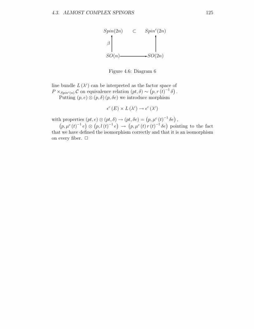
4.3. ALMOST COMPLEX SPINORS 125
Spin(2n) Spinc(2n)
SO(n) SO(2n)-
6 6β
⊂
Figure 4.6: Diagram 6
line bundle L (λc) can be interpreted as the factor space ofP ×Spinc(n) C on equivalence relation (pt, δ) ∼
(p, r (t)−1 δ
).
Putting (p, e)⊗ (p, δ) (p, δe) we introduce morphism
εc (E)× L (λc)→ εc (λc)
with properties (pt, e)⊗ (pt, δ)→ (pt, δe) =(p, µc (t)−1 δe
),(
p, µc (t)−1 e)⊗(p, l (t)−1 e
)→(p, µc (t) r (t)−1 δe
)pointing to the fact
that we have defined the isomorphism correctly and that it is an isomorphismon every fiber. 2

126 CHAPTER 4. ANISOTROPIC CLIFFORD STRUCTURES

Chapter 5
Spinors and Anisotropic Spaces
The purpose of this Chapter is to show how a corresponding abstract spinortechnique entailing notational and calculations advantages can be developedfor arbitrary splits of dimensions of a d-vector space F = hF ⊕ vF , wheredim hF = n and dim vF = m. For convenience we shall also present somenecessary coordinate expressions.
The problem of a rigorous definition of spinors on locally anisotropicspaces (anisotropic spinors, d–spinors) was posed and solved [163, 162, 189]in the framework of the formalism of Clifford and spinor structures on v–bundles provided with compatible nonlinear and distinguished connectionsand metric . We introduced d–spinors as corresponding objects of the Cliffordd–algebra C (F , G), defined for a d–vector space F in a standard manner(see, for instance, [83]) and proved that operations with C (F , G) can bereduced to calculations for C (hF , g) and C (vF , h) , which are usual Cliffordalgebras of respective dimensions 2n and 2m (if it is necessary we can usequadratic forms g and h correspondingly induced on hF and vF by a metricG (1.39)). Considering the orthogonal subgroup O(G) ⊂ GL(G) defined bya metric G we can define the d-spinor norm and parametrize d-spinors byordered pairs of elements of Clifford algebras C (hF , g) and C (vF , h) . Weemphasize that the splitting of a Clifford d-algebra associated to a v-bundleE is a straightforward consequence of the global decomposition defining aN-connection structure in E .
In this Chapter, as a rule, we shall omit proofs which in most cases aremechanical but rather tedious. We can apply the methods developed in[127, 128, 129, 91] in a straightforward manner on h- and v-subbundles inorder to verify the correctness of affirmations.
127

128 CHAPTER 5. SPINORS AND ANISOTROPIC SPACES
5.1 Anisotropic Clifford Algebras,
Spinors and Twistors
In order to relate the succeeding constructions with Clifford d-algebras [163,162] we consider a locally anisotropic frame decomposition of the metric(1.39):
Gαβ (u) = lαα (u) lββ (u)Gαβ, (5.1)
where the frame d-vectors and constant metric matrices are distinguished as
lαα (u) =
(ljj (u) 0
0 laa (u)
), Gαβ
(gij 0
0 hab
), (5.2)
gij and hab are diagonal matrices with gii = haa = ±1.To generate Clifford d-algebras we start with matrix equations
σασβ + σβσα = −GαβI, (5.3)
where I is the identity matrix, matrices σα (σ-objects) act on a d-vector spaceF = hF ⊕ vF and theirs components are distinguished as
σα =
(σα)
·γβ =
((σi)
·kj 0
0 (σa)·cb
), (5.4)
indices β,γ,... refer to spin spaces of type S = S(h) ⊕ S(v) and underlinedLatin indices j,k, ... and b, c, ... refer respectively to a h-spin space S(h) anda v-spin space S(v), which are correspondingly associated to a h- and v-decomposition of a v-bundle E(d). The irreducible algebra of matrices σα
of minimal dimension N × N, where N = N(n) + N(m), dimS(h)=N(n) anddimS(v)=N(m), has these dimensions
N(n) =
2(n−1)/2, n = 2k + 1
2n/2, n = 2k;
N(m) =
2(m−1)/2, m = 2k + 1
2m/2, m = 2k,
where k = 1, 2, ... .The Clifford d-algebra is generated by sums on n+ 1 elements of form
A1I +B iσi + C ijσij +Dijkσijk + ...

5.1. ANISOTROPIC SPINORS AND TWISTORS 129
and sums of m+ 1 elements of form
A2I +Baσa + C abσab +Dabcσabc + ...
with antisymmetric coefficients C ij = C [ij], C ab = C [ab], D ijk = D [ijk], Dabc =
D[abc], ... and matrices σij = σ[iσj], σab = σ[aσb], σijk = σ[iσjσk], ... . Really, we
have 2n+1 coefficients(A1, C
ij , D ijk, ...)
and 2m+1 coefficients(A2, C
ab, Dabc, ...)
of the Clifford algebra on F .
For simplicity, in this subsection, we shall present the necessary geometricconstructions only for h-spin spaces S(h) of dimensionN(n). Considerations fora v-spin space S(v) are similar but with proper characteristics for a dimensionN(m).
In order to define the scalar (spinor) product on S(h) we introduce intoconsideration this finite sum (because of a finite number of elements σ[ij...k]) :
(±)Eij
km = δikδ
jm +
2
1!(σi)
.ik(σi)
.jm +
22
2!(σij)
.ik(σ ij)
.jm +
23
3!(σijk)
.ik(σijk)
.jm + ...
(5.5)
which can be factorized as
(±)Eij
km = N(n)(±)εkm
(±)εij for n = 2k (5.6)
and
(+)Eij
km = 2N(n)εkmεij, (−)E
ij
km = 0 for n = 3(mod4), (5.7)
(+)Eij
km = 0, (−)Eij
km = 2N(n)εkmεij for n = 1(mod4).
Antisymmetry of σijk... and the construction of the objects (5.5),(5.6) and
(5.7) define the properties of ε-objects (±)εkm and εkm which have an eight-foldperiodicity on n (see details in [129] and, with respect to locally anisotropicspaces, [163]).
For even values of n it is possible the decomposition of every h-spin spaceS(h)into irreducible h-spin spaces S(h) and S′(h) (one considers splitting of h-indices, for instance, l= L⊕L′, m = M ⊕M ′, ...; for v-indices we shall writea = A⊕ A′, b = B ⊕B′, ...) and defines new ε-objects
εlm =1
2
((+)εlm +(−) εlm
)and εlm =
1
2
((+)εlm −(−) εlm
). (5.8)
We shall omit similar formulas for ε-objects with lower indices.

130 CHAPTER 5. SPINORS AND ANISOTROPIC SPACES
We can verify, by using expressions (5.7) and straightforward calculations,these parametrizations on symmetry properties of ε-objects (5.8)
εlm =
(εLM = εML 0
0 0
)and εlm =
(0 00 εLM = εML
)for n = 0(mod8);
εlm = −1
2(−)εlm = εml,where (+)εlm = 0, and (5.9)
εlm = −1
2(−)εlm = εmlfor n = 1(mod8);
εlm =
(0 0
εL′M 0
)and εlm =
(0 εLM ′
= −εM ′L
0 0
)for n = 2(mod8);
εlm = −1
2(+)εlm = −εml, where (−)εlm = 0, and
εlm =1
2(+)εlm = −εmlfor n = 3(mod8);
εlm =
(εLM = −εML 0
0 0
)and εlm =
(0 00 εLM = −εML
)for n = 4(mod8);
εlm = −1
2(−)εlm = −εml, where (+)εlm = 0, and
εlm = −1
2(−)εlm = −εmlfor n = 5(mod8);
εlm =
(0 0
εL′M 0
)and εlm =
(0 εLM ′
= εM′L
0 0
)for n = 6(mod8);
εlm =1
2(−)εlm = εml, where (+)εlm = 0, and
εlm = −1
2(−)εlm = εml for n = 7(mod8).
Let denote reduced and irreducible h-spinor spaces in a form pointing tothe symmetry of spinor inner products in dependence of values n = 8k + l(k = 0, 1, 2, ...; l = 1, 2, ...7) of the dimension of the horizontal subbundle(we shall write respectively 4 and for antisymmetric and symmetric inner
products of reduced spinors and ♦ = (4, ) and ♦ = (,4) for correspond-ing parametrizations of inner products, in brief i.p., of irreducible spinors;properties of scalar products of spinors are defined by ε-objects (5.9); weshall use for a general i.p. when the symmetry is not pointed out):

5.1. ANISOTROPIC SPINORS AND TWISTORS 131
S(h) (8k) = S ⊕ S′; (5.10)
S(h) (8k + 1) = S(−) (i.p. is defined by an (−)ε-object);
S(h) (8k + 2) = S = (S,S), orS ′ = (S′,S
′);
S(h) (8k + 3) = S(+)4 (i.p. is defined by an (+)ε-object);
S(h) (8k + 4) = S4 ⊕ S′4;
S(h) (8k + 5) = S(−)4 (i.p. is defined by an (−)ε-object),
S(h) (8k + 6) = S = (S,S), orS ′ = (S′,S
′);
S(h) (8k + 7) = S(+) (i.p. is defined by an (+)ε-object).
We note that by using corresponding ε-objects we can lower and riseindices of reduced and irreducible spinors (for n = 2, 6(mod4) we can excludeprimed indices, or inversely, see details in [127, 128, 129]).
The similar v-spinor spaces are denoted by the same symbols as in (5.10)provided with a left lower mark ”|” and parametrized with respect to thevalues m = 8k′ + l (k’=0,1,...; l=1,2,...,7) of the dimension of the verticalsubbundle, for example, as
S(v)(8k′) = S| ⊕ S′|,S(v) (8k + 1) = S(−)
| , ... (5.11)
We use ”˜”-overlined symbols,
S(h) (8k) = S ⊕ S ′, S(h) (8k + 1) = S(−) , ... (5.12)
and
S(v)(8k′) = S| ⊕ S ′|, S(v) (8k′ + 1) = S(−)
| , ... (5.13)
respectively for the dual to (5.10) and (5.11) spinor spaces.
The spinor spaces (5.10)-(5.13) are called the prime spinor spaces, in briefp-spinors . They are considered as building blocks of distinguished (n,m)–spinor spaces constructed in this manner:
(2.65)

132 CHAPTER 5. SPINORS AND ANISOTROPIC SPACES
S(,) = S ⊕ S′ ⊕ S| ⊕ S′|,S(,|) = S ⊕ S′ ⊕ S| ⊕ S′|,
S(, | ) = S ⊕ S′ ⊕ S| ⊕ S′|,S(|) = S ⊕ S′ ⊕ S| ⊕ S′|,
...............................................
S(4,4 ) = S(+)4 ⊕ S(+)
|4 , S(4,4 ) = S(+)4 ⊕ S(+)
|4 , (5.14)
................................
S(4|,♦ ) = S4 ⊕ S′ ⊕ S|♦,S(4|,♦ ) = S4 ⊕ S
′ ⊕ S♦| ,................................
Considering the operation of dualisation of prime components in (5.14) wecan generate different isomorphic variants of distinguished (n,m)–spinor spa-ces.
We define a d–spinor space S(n,m) as a direct sum of a horizontal and avertical spinor spaces of type (5.14), for instance,
S(8k,8k′) = S ⊕ S′ ⊕ S| ⊕ S′|,S(8k,8k′+1) = S ⊕ S′ ⊕ S(−)| , ...,
S(8k+4,8k′+5) = S4 ⊕ S′4 ⊕ S(−)|4 , ...
The scalar product on a S(n,m) is induced by (corresponding to fixed valuesof n and m ) ε-objects (5.9) considered for h- and v-components.
Having introduced d-spinors for dimensions (n,m) we can write out thegeneralization for locally anisotropic spaces of twistor equations [128] byusing the distinguished σ-objects (5.4):
(σ(α)..γ
|β|δωβ
δuβ)=
1
n+mGαβ(σε)
..γ
β
δωβ
δuε, (5.15)
where∣∣β∣∣ denotes that we do not consider symmetrization on this index. The
general solution of (5.15) on the d-vector space F looks like as
ωβ = Ωβ + uα(σα)..βε Πε, (5.16)
where Ωβ and Πε are constant d-spinors. For fixed values of dimensions n andm we mast analyze the reduced and irreducible components of h- and v-partsof equations (5.15) and their solutions (5.16) in order to find the symmetryproperties of a d-twistor Zα defined as a pair of d–spinors
Zα = (ωα, π′β),
where πβ′ = π(0)
β′ ∈ S(n,m) is a constant dual d-spinor. The problem of
definition of spinors and twistors on locally anisotropic spaces was firstlyconsidered in [189] (see also [156]) in connection with the possibility to extendthe equations (5.15) and their solutions (5.16), by using nearly autoparallelmaps, on curved, locally isotropic or anisotropic, spaces.

5.2. MUTUAL TRANSFORMS OF TENSORS AND SPINORS 133
5.2 Mutual Transforms of Tensors and Spi-
nors
The spinor algebra for spaces of higher dimensions can not be considered asa real alternative to the tensor algebra as for locally isotropic spaces of di-mensions n = 3, 4 [127, 128, 129]. The same holds true for locally anisotropicspaces and we emphasize that it is not quite convenient to perform a spinorcalculus for dimensions n,m >> 4. Nevertheless, the concept of spinors isimportant for every type of spaces, we can deeply understand the fundamen-tal properties of geometical objects on locally anisotropic spaces, and we shallconsider in this subsection some questions concerning transforms of d-tensorobjects into d-spinor ones.
5.2.1 Transformation of d-tensors into d-spinors
In order to pass from d-tensors to d-spinors we must use σ-objects (5.4)written in reduced or irreduced form (in dependence of fixed values ofdimensions n and m ):
(σα)·γβ , (σα)βγ, (σα)βγ, ..., (σa)
bc, ..., (σi)jk, ..., (σa)AA′, ..., (σi)II′, .... (5.17)
It is obvious that contracting with corresponding σ-objects (5.17) we canintroduce instead of d-tensors indices the d-spinor ones, for instance,
ωβγ = (σα)βγωα, ωAB′ = (σa)AB′ωa, ..., ζ i·j = (σk)i
·jζk, ....
For d-tensors containing groups of antisymmetric indices there is a moresimple procedure of theirs transforming into d-spinors because the objects
(σαβ...γ)δν , (σab...c)de, ..., (σ ij...k)II′, ... (5.18)
can be used for sets of such indices into pairs of d-spinor indices. Let us enu-merate some properties of σ-objects of type (5.18) (for simplicity we consider
only h-components having q indices i, j, k, ... taking values from 1 to n; theproperties of v-components can be written in a similar manner with respectto indices a, b, c... taking values from 1 to m):
(σi...j)kl is
symmetric on k, l for n− 2q ≡ 1, 7 (mod 8);
antisymmetric on k, l for n− 2q ≡ 3, 5 (mod 8)
(5.19)

134 CHAPTER 5. SPINORS AND ANISOTROPIC SPACES
for odd values of n, and an object
(σi...j)IJ((σi...j)
I′J ′)
is
symmetric on I, J (I ′, J ′) for n− 2q ≡ 0 (mod 8);
antisymmetric on I, J (I ′, J ′) for n− 2q ≡ 4 (mod 8)
(5.20)
or
(σi...j)IJ ′ = ±(σi...j)
J ′I n + 2q ≡ 6(mod8);n + 2q ≡ 2(mod8),
(5.21)
with vanishing of the rest of reduced components of the d-tensor (σi...j)kl with
prime/unprime sets of indices.
5.2.2 Fundamental d–spinors
We can transform every d-spinor ξα = (ξi, ξa) into a corresponding d-tensor.For simplicity, we consider this construction only for a h-component ξi on ah-space being of dimension n. The values
ξαξβ(σi...j)αβ (n is odd) (5.22)
or
ξIξJ(σi...j)IJ
(or ξI′ξJ ′(σi...j)I′J ′
)(n is even) (5.23)
with a different number of indices i...j, taken together, defines the h-spinorξi to an accuracy to the sign. We emphasize that it is necessary to chooseonly those h-components of d-tensors (5.22) (or (5.23)) which are symmetricon pairs of indices αβ (or IJ (or I ′J ′ )) and the number q of indices i...jsatisfies the condition (as a respective consequence of the properties (5.19)and/or (5.20), (5.21))
n− 2q ≡ 0, 1, 7 (mod 8). (5.24)
Of special interest is the case when
q =1
2(n± 1) (n is odd) (5.25)
or
q =1
2n (n is even) . (5.26)

5.3. ANISOTROPIC SPINOR DIFFERENTIAL GEOMETRY 135
If all expressions (5.22) and/or (5.23) are zero for all values of q with theexception of one or two ones defined by the condition (5.25) (or (5.26)), the
value ξ i (or ξI (ξI′)) is called a fundamental h-spinor. Defining in a similarmanner the fundamental v-spinors we can introduce fundamental d-spinorsas pairs of fundamental h- and v-spinors. Here we remark that a h(v)-spinor
ξ i (ξa) (we can also consider reduced components) is always a fundamentalone for n(m) < 7, which is a consequence of (5.24)).
Finally, in this section, we note that the geometry of fundamental h- andv-spinors is similar to that of usual fundamental spinors (see Appendix to themonograph [129]). We omit such details in this work, but emphasize thatconstructions with fundamental d-spinors, for a locally anisotropic space,must be adapted to the corresponding global splitting by N-connection ofthe space.
5.3 Anisotropic Spinor Differential Geome-
try
The goal of the section is to formulate the differential geometry of d-spinorsfor locally anisotropic spaces.
We shall use denotations of type
vα = (vi, va) ∈ σα = (σi, σa) and ζα = (ζ i, ζa) ∈ σα = (σi, σa)
for, respectively, elements of modules of d-vector and irreduced d-spinor fields(see details in [163]). D-tensors and d-spinor tensors (irreduced or reduced)will be interpreted as elements of corresponding σ -modules, for instance,
qαβ... ∈ σα
β, ψα γ
β ... ∈ σα γ
β ... , ξII′
JK ′N ′ ∈ σII′JK ′N ′ , ...
We can establish a correspondence between the d–metric gαβ (1.39) andd-spinor metric εαβ ( ε-objects (5.9) for both h- and v-subspaces of E ) of alocally anisotropic space E by using the relation
gαβ = − 1
N(n) +N(m)((σ(α(u))α1β
1(σβ)(u))β
2α2)εα1α2
εβ1β
2, (5.27)
where
(σα(u))νγ = lαα(u)(σα)νγ, (5.28)
which is a consequence of formulas (5.1)-(5.6). In brief we can write (5.27)as
gαβ = εα1α2εβ
1β
2(5.29)

136 CHAPTER 5. SPINORS AND ANISOTROPIC SPACES
if the σ-objects are considered as a fixed structure, whereas ε-objects aretreated as caring the metric ”dynamics ” , on locally anisotropic space–times. This variant is used, for instance, in the so-called 2-spinor geometry[128, 129] and should be preferred if we have to make explicit the algebraicsymmetry properties of d-spinor objects. An alternative way is to consideras fixed the algebraic structure of ε-objects and to use variable componentsof σ-objects of type (5.28) for developing a variational d-spinor approach togravitational and matter field interactions on locally anisotropic spaces ( thespinor Ashtekar variables [20] are introduced in this manner).
We note that a d–spinor metric
εντ =
(εij 0
0 εab
)on the d-spinor space S = (S(h),S(v)) can have symmetric or antisymmetric h(v) -components εij (εab) , see ε-objects (5.9). For simplicity, in this section (inorder to avoid cumbersome calculations connected with eight-fold periodicityon dimensions n and m of a locally anisotropic space E ) we shall developa general d-spinor formalism only by using irreduced spinor spaces S(h) andS(v).
5.4 D-covariant derivation
Let E be a locally anisotropic space. We define the action on a d-spinor of ad-covariant operator
5α = (5i,5a) = (σα)α1α25α1α2 =((σi)
i1i25i1i2 , (σa)a1a25a1a2
)(in brief, we shall write
5α = 5α1α2 = (5i1i2 , 5a1a2 ))
as a map
5α1α2: σβ → σ
βα = σ
βα1α2
satisfying conditions
5α(ξβ + ηβ) = 5αξβ +5αη
β,
and
5α(fξβ) = f 5α ξβ + ξβ 5α f
5.4. D-COVARIANT DERIVATION 137
for every ξβ, ηβ ∈ σβ and f being a scalar field on E . It is also required thatone holds the Leibnitz rule
(5αζβ)ηβ = 5α(ζβηβ)− ζβ 5α η
β
and that 5α is a real operator, i.e. it commuters with the operation ofcomplex conjugation:
5αψαβγ... = 5α(ψαβγ...).
Let now analyze the question on uniqueness of action on d-spinors of anoperator 5α satisfying necessary conditions . Denoting by 5(1)
α and 5α twosuch d-covariant operators we consider the map
(5(1)α −5α) : σβ → σ
βα∞α∈ . (5.30)
Because the action on a scalar f of both operators 5(1)α and 5α must be
identical, i.e.
5(1)α f = 5αf, (5.31)
the action (5.30) on f = ωβξβ must be written as
(5(1)α −5α)(ωβξ
β) = 0.
In consequence we conclude that there is an element Θγ
α1α2β ∈ σγ
α1α2β for
which
5(1)α1α2
ξγ = 5α1α2ξγ + Θ
γ
α1α2β ξβ (5.32)
and
5(1)α1α2
ωβ = 5α1α2ωβ −Θ
γ
α1α2β ωγ .
The action of the operator (5.30) on a d-vector vβ = vβ1β
2 can be written byusing formula (5.32) for both indices β
1and β
2:
(5(1)α −5α)vβ
1β
2 = Θβ
1αγ vγβ
2 + Θβ
2αγ vβ
1γ
= (Θβ
1αγ
1δ
β2
γ2
+ Θβ
2αγ
1δ
β1
γ2
)vγ1γ2 = Qβ
αγvγ,
where
Qβαγ = Q
β1β
2α1α2 γ
1γ2
= Θβ
1αγ
1δ
β2
γ2
+ Θβ
2αγ
1δ
β1
γ2
. (5.33)

138 CHAPTER 5. SPINORS AND ANISOTROPIC SPACES
The d-commutator 5[α5β] defines the d–torsion. So, applying operators
5(1)[α 5
(1)β] and 5[α5β] on f = ωβξ
β we can write
T(1)γ
αβ − Tγαβ = Qγ
βα −Qγαβ
with Qγαβ from (5.33).
The action of operator 5(1)α on d-spinor tensors of type χ
β1β
2...
α1α2α3...
must be constructed by using formula (5.32) for every upper index β1β
2...
and formula (5.33) for every lower index α1α2α3... .
5.5 Infeld - van der Waerden coefficients
Let
δ αα =
(δ i1 , δ i
2 , ..., δ iN(n), δ
a1 , δ a
2 , ..., δ iN(m)
)be a d-spinor basis. The dual to it basis is denoted as
δ αα =
(δ 1i , δ 2
i , ..., δN(n)
i , δ 1i , δ 2
i , ..., δN(m)
i
).
A d-spinor κα ∈ σ α has components κα = καδ αα . Taking into account that
δ αα δ
β
β 5αβ = 5αβ,
we write out the components 5αβ κγ as
δ αα δ
β
β δγ
γ 5αβ κγ = δ τ
ε δγ
τ 5αβ κε + κε δ
γε 5αβ δ
εε
= 5αβκγ + κεγ
γ
αβε, (5.34)
where the coordinate components of the d-spinor connection γγ
αβε are definedas
γγ
αβε
.= δ
γτ 5αβ δ
τε . (5.35)
We call the Infeld - van der Waerden d-symbols a set of σ-objects (σα)αβ
parametrized with respect to a coordinate d-spinor basis. Defining
5α = (σα)αβ 5αβ,
introducing denotations
γγατ
.= γγ
αβτ (σα)αβ

5.5. INFELD - VAN DER WAERDEN COEFFICIENTS 139
and using properties (5.34) we can write relations
lαα δβ
β 5α κβ = 5ακ
β + κδ γβ
αδ (5.36)
and
lαα δβ
β 5α µβ = 5α µβ − µδγδαβ (5.37)
for d-covariant derivations 5α κβ and 5α µβ.
We can consider expressions similar to (5.36) and (5.37) for values havingboth types of d-spinor and d-tensor indices, for instance,
lαα lγγ δ
δδ 5α θ
γδ = 5αθ
γδ − θ γ
ε γεαδ + θ τ
δ Γ γατ
(we can prove this by a straightforward calculation of the derivation5α(θ τ
ε δ εδ lγτ )).
Now we shall consider some possible relations between components ofd-connections γε
αδ and Γ γατ and derivations of (σα)αβ . We can write
Γαβγ = lαα 5γ l
αβ = lαα 5γ (σβ)ετ = lαα 5γ ((σβ)ετδ ε
ε δτ
τ )
= lααδα
α δ εε 5γ (σβ)αε + lαα(σβ)ετ (δ τ
τ 5γ δε
ε + δ εε 5γ δ
ττ )
= lαετ 5γ (σβ)ετ + lαµνδµ
ε δν
τ (σβ)ετ (δ ττ 5γ δ
εε + δ ε
ε 5γ δτ
τ ),
where lαα = (σετ )α , from which it follows
(σα)µν(σαβ)βΓαγβ = (σαβ)β 5γ (σα)µν + δ ν
β γµγα + δ
µα γ
νγβ.
Connecting the last expression on β and ν and using an orthonormalized
d-spinor basis when γβ
γβ = 0 (a consequence from (5.35)) we have
γµγα =
1
N(n) +N(m)(Γ
µβ
γ αβ − (σαβ)β 5γ (σβ)µβ), (5.38)
where
Γµβ
γ αβ = (σα)µβ(σαβ)βΓαγβ. (5.39)
We also note here that, for instance, for the canonical and Berwald con-nections, Christoffel d-symbols we can express d-spinor connection (5.39)through corresponding locally adapted derivations of components of metricand N-connection by introducing respectively the coefficients of the Barwald,canonical or another type d–connections.

140 CHAPTER 5. SPINORS AND ANISOTROPIC SPACES
5.6 D-spinors of Anisotropic Curvature and
Torsion
The d-tensor indices of the commutator ∆αβ can be transformed into d-spinorones:
2αβ = (σαβ)αβ∆αβ = (2ij ,2ab), (5.40)
with h- and v-components,
2ij = (σαβ)ij∆αβ and 2ab = (σαβ)ab∆αβ,
being symmetric or antisymmetric in dependence of corresponding values ofdimensions n and m (see eight-fold parametizations (5.18)–(5.20)). Consid-ering the actions of operator (5.40) on d-spinors πγ and µγ we introduce the
d-spinor curvature Xγ
δ αβ as to satisfy equations
2αβ πγ = X
γ
δ αβπδ (5.41)
and
2αβ µγ = X δγ αβµδ.
The gravitational d-spinor Ψαβγδ is defined by a corresponding symmetriza-tion of d-spinor indices:
Ψαβγδ = X(α|β|γδ). (5.42)
We note that d-spinor tensors Xγ
δ αβ and Ψαβγδ are transformed into similar
2-spinor objects on locally isotropic spaces [128, 129] if we consider vanishingof the N-connection structure and a limit to a locally isotropic space.
Putting δγ
γ instead of µγ in (5.41) and using (5.42) we can expressrespectively the curvature and gravitational d-spinors as
Xγδαβ = δδτ2αβδτ
γ
and
Ψγδαβ = δδτ2(αβδτ
γ) .
The d-spinor torsion Tγ1γ2
αβ is defined similarly as for d-tensors) by
using the d-spinor commutator (5.40) and equations
2αβf = Tγ1γ2
αβ 5γ1γ2f.

5.6. D-SPINORS OF ANISOTROPIC CURVATURE AND TORSION141
The d-spinor components Rδ1δ2
γ1γ2
αβ of the curvature d-tensor R δγ αβ
can be computed by using the relations (5.39), (5.40) and (5.42) as to satisfythe equations (the d-spinor analogous of equations (1.79) )
(2αβ − Tγ1γ2
αβ5γ1γ2)V δ1δ2 = R
δ1δ2γ1γ2
αβVγ1γ2 , (5.43)
here d-vector V γ1γ2 is considered as a product of d-spinors, i.e. V γ
1γ2 =
νγ1µγ
2 . We find
Rδ1δ2
γ1γ2
αβ =(X
δ1γ1
αβ + Tτ1τ2
αβ γδ1τ1τ2γ
1
)δ δ2γ2
(5.44)
+(X
δ2γ2
αβ + Tτ1τ2
αβ γδ2τ1τ2γ
2
)δ δ1γ1
.
It is convenient to use this d-spinor expression for the curvature d-tensor
Rδ1δ2
γ1γ2
α1α2β1β
2=
(X
δ1γ1
α1α2β1β
2+ T
τ1τ2α1α2β
1β
2γδ1
τ1τ2γ1
)δ δ2γ2
+(X
δ2γ2
α1α2β1β
2+ T
τ1τ2α1α2β
1β
2γδ2
τ1τ2γ2
)δ δ1γ1
in order to get the d-spinor components of the Ricci d-tensor
Rγ1γ2α1α2
= Rδ1δ2
γ1γ2
α1α2δ1δ2= X
δ1γ1
α1α2δ1γ2+ T
τ1τ2α1α2δ1γ
2γδ1
τ1τ2γ1
+Xδ2
γ2
α1α2δ1γ2+ T
τ1τ2α1α2γ
1δ2γδ2
τ1τ2γ2
(5.45)
and this d-spinor decomposition of the scalar curvature:
q←−R = Rα1α2
α1α2= X
α1δ1 α2α1 δ1α2
+ Tτ1τ2α1 α2
α2δ1γδ1
τ1τ2α1(5.46)
+Xα2δ2α1
α2δ2α1+ T
τ1τ2 α2α1α1 δ2
γδ2τ1τ2α2
.
Putting (2.96) and (2.97) into (2.43) and, correspondingly, (2.41) we findthe d-spinor components of the Einstein and Φαβ d-tensors:
←−G γα =
←−G γ
1γ2α1α2
= Xδ1
γ1
α1α2δ1γ2+ T
τ1τ2α1α2δ1γ
2γδ1
τ1τ2γ1
(5.47)
+Xδ2
γ2
α1α2δ1γ2+ T
τ1τ2α1α2γ
1δ2γδ2
τ1τ2γ2
−1
2εγ
1α1εγ
2α2
[Xβ
1µ
1β
2β
1µ
1β
2+ T
τ1τ2β1
β2
β2µ
1γ
µ1
τ1τ2β1
+Xβ
2µ
2ν1
β2µ
2ν1
+ Tτ1τ2 β
2β
1β
1δ2γ
δ2τ1τ2β
2]

142 CHAPTER 5. SPINORS AND ANISOTROPIC SPACES
and
Φγα = Φγ1γ2α1α2
=1
2(n+m)εγ
1α1εγ
2α2
[Xβ
1µ
1β
2β
1µ
1β
2(5.48)
+Tτ1τ2β
1β
2
β2µ
1γ
µ1
τ1τ2β1+X
β2µ
2ν1
β2µ
2ν1
+ Tτ1τ2 β
2β
1
β1
δ2γ
δ2
τ1τ2β2]
−1
2[X
δ1γ1
α1α2δ1γ2+ T
τ1τ2α1α2δ1γ
2γδ1
τ1τ2γ1
+Xδ2
γ2
α1α2δ1γ2+ T
τ1τ2α1α2γ
1δ2γδ2
τ1τ2γ2].
The components of the conformal Weyl d-spinor can be computed byputting d-spinor values of the curvature (5.44) and Ricci (5.44) d-tensorsinto corresponding expression for the d-tensor (1.82). We omit this calculusin this work.

Chapter 6
Anisotropic Spinors and FieldEquations
The problem of formulation gravitational and gauge field equations on differ-ent types of locally anisotropic spaces is considered, for instance, in [109, 27,19] and [186]. In this section we shall introduce the basic field equations forgravitational and matter field locally anisotropic interactions in a generalizedform for generic locally anisotropic spaces.
6.1 Anisotropic Scalar Field Interactions
Let ϕ (u) = (ϕ1 (u) , ϕ2 (u) ,..., ϕk (u)) be a complex k-component scalar fieldof mass µ on locally anisotropic space E . The d-covariant generalization of theconformally invariant (in the massless case) scalar field equation [128, 129]can be defined by using the d’Alambert locally anisotropic operator [4, 168]2 = DαDα, where Dα is a d-covariant derivation on E constructed, forsimplicity, by using Christoffel d–simbols (all formulas for field equations andconservation values can be deformed by using corresponding defrormation d–tensors P α
βγ from the Cristoffel d–simbols, or the canonical d–connection toa general d-connection into consideration):
(2 +n +m− 2
4(n+m− 1)
←−R + µ2)ϕ (u) = 0. (6.1)
We must change d-covariant derivation Dα into Dα = Dα + ieAα and takeinto account the d-vector current
J (0)α (u) = i((ϕ (u)Dαϕ (u)−Dαϕ (u))ϕ (u))
143

144 CHAPTER 6. ANISOTROPIC SPINORS AND FIELD EQUATIONS
if interactions between locally anisotropic electromagnetic field ( d-vectorpotential Aα ), where e is the electromagnetic constant, and charged scalarfield ϕ are considered. The equations (6.1) are (locally adapted to the N-connection structure) Euler equations for the Lagrangian
L(0) (u) =√|g|[gαβδαϕ (u) δβϕ (u)−
(µ2 +
n+m− 2
4(n+m− 1)
)ϕ (u)ϕ (u)
],
(6.2)
where |g| = detgαβ .
The locally adapted variations of the action with Lagrangian (6.2) onvariables ϕ (u) and ϕ (u) leads to the locally anisotropic generalization of theenergy-momentum tensor,
E(0,can)αβ (u) = δαϕ (u) δβϕ (u) + δβϕ (u) δαϕ (u)− 1√
|g|gαβL(0) (u) , (6.3)
and a similar variation on the components of a d-metric (1.39) leads to asymmetric metric energy-momentum d-tensor,
E(0)αβ (u) = E
(0,can)(αβ) (u)− n+m− 2
2(n+m− 1)
[R(αβ) +D(αDβ) − gαβ2
]ϕ (u)ϕ (u) .
(6.4)
Here we note that we can obtain a nonsymmetric energy-momentum d-tensorif we firstly vary on Gαβ and than impose the constraints of compatibilitywith the N-connection structure. We also conclude that the existence of aN-connection in v-bundle E results in a nonequivalence of energy-momentumd-tensors (6.3) and (6.4), nonsymmetry of the Ricci tensor (see (1.77)),nonvanishing of the d-covariant derivation of the Einstein d-tensor (1.85),Dα←−G αβ 6= 0 and, in consequence, a corresponding breaking of conservation
laws on locally anisotropic spaces when DαEαβ 6= 0 [108, 109]. The prob-
lem of formulation of conservation laws on locally anisotropic spaces is dis-cussed in details and two variants of its solution (by using nearly autoparallelmaps and tensor integral formalism on locally anisotropic multispaces) areproposed in [168]. In this section we shall present only straightforward gen-eralizations of field equations and necessary formulas for energy-momentumd-tensors of matter fields on E considering that it is naturally that the con-servation laws (usually being consequences of global, local and/or intrinsicsymmetries of the fundamental space-time and of the type of field interac-tions) have to be broken on locally anisotropic spaces.

6.2. ANISOTROPIC PROCA EQUATIONS 145
6.2 Anisotropic Proca equations
Let consider a d-vector field ϕα (u) with mass µ2 (locally anisotropic Procafield ) interacting with exterior locally anisotropic gravitational field. Fromthe Lagrangian
L(1) (u) =√|g|[−1
2fαβ (u) fαβ (u) + µ2ϕα (u)ϕα (u)
], (6.5)
where fαβ = Dαϕβ − Dβϕα, one follows the Proca equations on locallyanisotropic spaces
Dαfαβ (u) + µ2ϕβ (u) = 0. (6.6)
Equations (6.6) are a first type constraints for β = 0. Acting with Dα on(6.6), for µ 6= 0 we obtain second type constraints
Dαϕα (u) = 0. (6.7)
Putting (6.7) into (6.6) we obtain second order field equations with re-spect to ϕα :
2ϕα (u) +Rαβϕβ (u) + µ2ϕα (u) = 0. (6.8)
The energy-momentum d-tensor and d-vector current following from the (6.8)can be written as
E(1)αβ (u) = −gετ
(fβτfαε + fαεfβτ
)+ µ2
(ϕαϕβ + ϕβϕα
)− gαβ√
|g|L(1) (u) .
and
J (1)α (u) = i
(fαβ (u)ϕβ (u)− ϕβ (u) fαβ (u)
).
For µ = 0 the d-tensor fαβ and the Lagrangian (6.5) are invariant withrespect to locally anisotropic gauge transforms of type
ϕα (u)→ ϕα (u) + δαΛ (u) ,
where Λ (u) is a d-differentiable scalar function, and we obtain a locallyanisotropic variant of Maxwell theory.

146 CHAPTER 6. ANISOTROPIC SPINORS AND FIELD EQUATIONS
6.3 Anisotropic Gravitons and Backgrounds
Let a massless d-tensor field hαβ (u) is interpreted as a small perturbationof the locally anisotropic background metric d-field gαβ (u) . Considering, forsimplicity, a torsionless background we have locally anisotropic Fierz-Pauliequations
2hαβ (u) + 2Rταβν (u) hτν (u) = 0 (6.9)
and d-gauge conditions
Dαhαβ (u) = 0, h (u) ≡ hα
β(u) = 0, (6.10)
where Rταβν (u) is curvature d-tensor of the locally anisotropic backgroundspace (these formulae can be obtained by using a perturbation formalism withrespect to hαβ (u) developed in [75]; in our case we must take into accountthe distinguishing of geometrical objects and operators on locally anisotropicspaces).
We note that we can rewrite d-tensor formulas (6.1)-(6.10) into similard-spinor ones by using formulas (5.27)–(5.29), (5.39), (5.41) and (5.45)–(6.6)(for simplicity, we omit these considerations in this work).
6.4 Anisotropic Dirac Equations
Let denote the Dirac d-spinor field on E as ψ (u) = (ψα (u)) and consider asthe generalized Lorentz transforms the group of automorphysm of the metricGαβ (see the locally anisotropic frame decomposition of d-metric (5.3)). Thed-covariant derivation of field ψ (u) is written as
−→5αψ =
[δα +
1
4Cαβγ (u) lαα (u)σβσγ
]ψ, (6.11)
where coefficients Cαβγ = (Dγlαα) lβαl
γγ generalize for locally anisotropic spaces
the corresponding Ricci coefficients on Riemannian spaces [60]. Using σ-objects σα (u) (see (5.28) and (5.4)) we define the Dirac equations on locallyanisotropic spaces:
(iσα (u)−→5α − µ)ψ = 0, (6.12)
which are the Euler equations for the Lagrangian
L(1/2) (u) =√|g|[ψ+ (u)σα (u)
−→5αψ (u) (6.13)
−(−→5αψ
+ (u))σα (u)ψ (u)]− µψ+ (u)ψ (u),

6.5. YANG-MILLS EQUATIONS IN ANISOTROPIC SPINOR FORM147
where ψ+ (u) is the complex conjugation and transposition of the columnψ (u) .
From (6.13) we obtain the d-metric energy-momentum d-tensor
E(1/2)αβ (u) =
i
4[ψ+ (u)σα (u)
−→5βψ (u) + ψ+ (u)σβ (u)−→5αψ (u)
−(−→5αψ
+ (u))σβ (u)ψ (u)− (−→5βψ
+ (u))σα (u)ψ (u)]
and the d-vector source
J (1/2)α (u) = ψ+ (u)σα (u)ψ (u) .
We emphasize that locally anisotropic interactions with exterior gauge fieldscan be introduced by changing the locally anisotropic partial derivation from(6.11) in this manner:
δα → δα + ie?Bα, (6.14)
where e? and Bα are respectively the constant d-vector potential of locallyanisotropic gauge interactions on locally anisotropic spaces (see [186] and thenext section).
6.5 Yang-Mills Equations in Anisotropic Spi-
nor Form
We consider a v-bundle BE , πB : B → E , on locally anisotropic space E .Additionally to d-tensor and d-spinor indices we shall use capital Greek let-ters, Φ,Υ,Ξ,Ψ, ... for fibre (of this bundle) indices (see details in [128, 129]for the case when the base space of the v-bundle πB is a locally isotropicspace-time). Let 5
αbe, for simplicity, a torsionless, linear connection in BE
satisfying conditions:
5α
: ΥΘ → ΥΘα
[or ΞΘ → ΞΘ
α
],
5α
(λΘ + νΘ
)= 5
αλΘ +5
ανΘ,
5α
(fλΘ) = λΘ5αf + f5
αλΘ, f ∈ ΥΘ [or ΞΘ],
where by ΥΘ(
ΞΘ)
we denote the module of sections of the real (complex)v-bundle BE provided with the abstract index Θ. The curvature of connection5
αis defined as
K ΘαβΩ λΩ =
(5
α5
β−5
β5
α
)λΘ.

148 CHAPTER 6. ANISOTROPIC SPINORS AND FIELD EQUATIONS
For Yang-Mills fields as a rule one considers that BE is enabled witha unitary (complex) structure (complex conjugation changes mutually theupper and lower Greek indices). It is useful to introduce instead of K Θ
αβΩ
a Hermitian matrix F ΘαβΩ = i K Θ
αβΩ connected with components of theYang-Mills d-vector potential B Φ
αΞ according the formula:
1
2F Φ
αβΞ = 5[αB Φ
β]Ξ − iB Φ[α|Λ|B
Λβ]Ξ , (6.15)
where the locally anisotropic space indices commute with capital Greek in-dices. The gauge transforms are written in the form:
B ΦαΘ 7→ B Φ
αΘ= B Φ
αΘ s ΦΦ q Θ
Θ+ is Φ
Θ 5αq ΘΘ
,
F ΦαβΞ 7→ F Φ
αβΞ= F Φ
αβΞ s ΦΦ q Ξ
Ξ,
where matrices s ΦΦ and q Ξ
Ξare mutually inverse (Hermitian conjugated in
the unitary case). The Yang-Mills equations on torsionless locally anisotropicspaces [186] (see details in the next Chapter) are written in this form:
5αF ΨαβΘ = J Ψ
β Θ , (6.16)
5[αF Ξ
βγ]Θ = 0. (6.17)
We must introduce deformations of connection of type,5?
α−→ 5
α+ Pα, (the deformation d-tensor Pα is induced by the torsion
in v-bundle BE) into the definition of the curvature of locally anisotropicgauge fields (6.15) and motion equations (6.16) and (6.17) if interactions aremodeled on a generic locally anisotropic space.
Now we can write out the field equations of the Einstein-Cartan theoryin the d-spinor form. So, for the Einstein equations (1.84) we have
←−G γ
1γ2α1α2
+ λεγ1α1εγ
2α2
= κEγ1γ2α1α2
,
with←−G γ
1γ2α1α2
from (5.47), or, by using the d-tensor (5.48),
Φγ1γ2α1α2
+ (
←−R
4− λ
2)εγ
1α1εγ
2α2
= −κ2Eγ
1γ2α1α2
,
which are the d-spinor equivalent of the equations (1.86). These equationsmust be completed by the algebraic equations (1.87) for the d-torsion and d-spin density with d-tensor indices changed into corresponding d-spinor ones.

Part III
Higher Order AnisotropicSpinors
149


151
The theory of anisotropic spinors formulated in the Part II is extended forhigher order anisotropic (ha) spaces. In brief, such spinors will be called ha–spinors which are defined as some Clifford ha–structures defined with respectto a distinguished quadratic form (1.43) on a hvc–bundle. For simplicity, thebulk of formulas will be given with respect to higher order vector bundles. Torewrite such formulas for hvc–bundles is to consider for the ”dual” shells ofhigher order anisotropy some dual vector spaces and associated dual spinors.

152

Chapter 7
Clifford Ha–Structures
7.1 Distinguished Clifford Algebras
The typical fiber of dv–bundle ξd , πd : HE ⊕ V1E ⊕ ... ⊕ VzE → E isa d-vector space, F = hF ⊕ v1F⊕... ⊕ vzF , split into horizontal hF andverticals vpF , p = 1, ..., z subspaces, with a bilinear quadratic form G(g, h)induced by a hvc–bundle metric (1.43). Clifford algebras (see, for example,Refs. [83, 154, 129]) formulated for d-vector spaces will be called Cliffordd-algebras [163, 162, 189]. We shall consider the main properties of Cliffordd–algebras. The proof of theorems will be based on the technique developedin Ref. [83] correspondingly adapted to the distinguished character of spacesin consideration.
Let k be a number field (for our purposes k = R or k = C,R and C,are, respectively real and complex number fields) and define F , as a d-vectorspace on k provided with nondegenerate symmetric quadratic form (metric)G. Let C be an algebra on k (not necessarily commutative) and j : F → Ca homomorphism of underlying vector spaces such that j(u)2 = G(u) · 1 (1is the unity in algebra C and d-vector u ∈ F). We are interested in definitionof the pair (C, j) satisfying the next universitality conditions. For everyk-algebra A and arbitrary homomorphism ϕ : F → A of the underlying d-vector spaces, such that (ϕ(u))2 → G (u)·1, there is a unique homomorphismof algebras ψ : C → A transforming the diagram 1 into a commutative one.
The algebra solving this problem will be denoted as C (F , A) [equivalentlyas C (G) or C (F)] and called as Clifford d–algebra associated with pair(F , G) .
Theorem 7.1. The above-presented diagram has a unique solution (C, j) upto isomorphism.
Proof: (We adapt for d-algebras that of Ref. [83], p. 127 and extend
153

154 CHAPTER 7. CLIFFORD HA–STRUCTURES
for higher order anisotropies a similar proof presented in the Part II). For auniversal problem the uniqueness is obvious if we prove the existence of solu-tion C (G) . To do this we use tensor algebra L(F ) = ⊕Lpr
qs (F) =⊕∞i=0Ti (F) ,
where T 0 (F) = k and T i (F) = k and T i (F) = F⊗...⊗F for i > 0. Let I (G)be the bilateral ideal generated by elements of form ε (u) = u⊗ u−G (u) · 1where u ∈ F and 1 is the unity element of algebra L (F) . Every elementfrom I (G) can be written as
∑i λiε (ui)µi, where λi, µi ∈ L(F) and ui ∈ F .
Let C (G) =L(F)/I (G) and define j : F → C (G) as the composition ofmonomorphism i : F → L1(F) ⊂ L(F) and projection p : L (F) → C (G) .In this case pair (C (G) , j) is the solution of our problem. From the generalproperties of tensor algebras the homomorphism ϕ : F → A can be extendedto L(F) , i.e., the diagram 2 is commutative, where ρ is a monomorphismof algebras. Because (ϕ (u))2 = G (u) · 1, then ρ vanishes on ideal I (G) andin this case the necessary homomorphism τ is defined. As a consequence ofuniqueness of ρ, the homomorphism τ is unique.
Tensor d–algebra L(F) can be considered as a Z/2 graded algebra. Re-ally, let us introduce L(0)(F) =
∑∞i=1 T
2i (F) and L(1)(F) =∑∞
i=1 T2i+1 (F) .
Setting I(α) (G) = I (G)∩L(α)(F). Define C(α) (G) as p(L(α)(F)
), where p :
L (F)→ C (G) is the canonical projection. Then C (G) = C(0) (G)⊕C(1) (G)and in consequence we obtain that the Clifford d–algebra is Z/2 graded.
It is obvious that Clifford d-algebra functorially depends on pair (F , G) .If f : F → F ′ is a homomorphism of k-vector spaces, such that G′ (f(u)) =G (u) , where G and G′ are, respectively, metrics on F and F ′, then f inducesan homomorphism of d-algebras
C (f) : C (G)→ C (G′)
with identities C (ϕ · f) = C (ϕ)C (f) and C (IdF) = IdC(F).If Aα and Bβ are Z/2–graded d–algebras, then their graded tensorial
product Aα⊗Bβ is defined as a d-algebra for k-vector d-space Aα⊗Bβ withthe graded product induced as (a⊗ b) (c⊗ d) = (−1)αβ ac⊗bd, where b ∈ Bα
and c ∈ Aα (α, β = 0, 1) .Now we re–formulate for d–algebras the Chevalley theorem [45]:
Theorem 7.2. The Clifford d-algebra
C (hF ⊕ v1F ⊕ ...⊕ vzF , g + h1 + ...+ hz)
is naturally isomorphic to C(g)⊗ C (h1)⊗ ...⊗ C (hz) .
Proof. Let n : hF → C (g) and n′(p) : v(p)F → C(h(p)
)be canonical
maps and map
m : hF ⊕ v1F ⊕ ...⊕ vzF → C(g)⊗ C (h1)⊗ ...⊗ C (hz)

7.1. DISTINGUISHED CLIFFORD ALGEBRAS 155
is defined as
m(x, y(1), ..., y(z)) =
n(x)⊗ 1⊗ ...⊗ 1 + 1⊗ n′(y(1))⊗ ...⊗ 1 + 1⊗ ...⊗ 1⊗ n′(y(z)),
x ∈ hF , y(1) ∈ v(1)F , ..., y(z) ∈ v(z)F . We have(m(x, y(1), ..., y(z))
)2=
[(n (x))2 +
(n′(y(1)
))2+ ...+
(n′(y(z)
))2] · 1= [g (x) + h
(y(1)
)+ ... + h
(y(z)
)].
Taking into account the universality property of Clifford d-algebras we con-clude that m1 + ... +mz induces the homomorphism
ζ : C (hF ⊕ v1F ⊕ ...⊕ vzF , g + h1 + ...+ hz)→C (hF , g) ⊗C (v1F , h1) ⊗...C (vzF , hz) .
We also can define a homomorphism
υ : C (hF , g) ⊗C(v1F , h(1)
)⊗...⊗C
(vzF , h(z)
)→
C(hF ⊕ v1F ⊕ ...⊕ vzF , g + h(1) + ...+ h(z)
)by using formula υ
(x⊗ y(1) ⊗ ...⊗ y(z)
)= δ (x) δ′(1)
(y(1)
)...δ′(z)
(y(z)
), where
homomorphysms δ and δ′(1), ..., δ′(z) are, respectively, induced by imbeddings
of hF and v1F into hF ⊕ v1F ⊕ ...⊕ vzF :
δ : C (hF , g)→ C(hF ⊕ v1F ⊕ ...⊕ vzF , g + h(1) + ...+ h(z)
),
δ′(1) : C(v1F , h(1)
)→ C
(hF ⊕ v1F ⊕ ...⊕ vzF , g + h(1) + ... + h(z)
),
...................................
δ′(z) : C(vzF , h(z)
)→ C
(hF ⊕ v1F ⊕ ...⊕ vzF , g + h(1) + ...+ h(z)
).
Superpositions of homomorphisms ζ and υ lead to identities
υζ = IdC(hF ,g)⊗C(v1F ,h(1))⊗...⊗C(vzF ,h(z)), (7.1)
ζυ = IdC(hF ,g)⊗C(v1F ,h(1))⊗...⊗C(vzF ,h(z)).
Really, d-algebra C(hF ⊕ v1F ⊕ ...⊕ vzF , g + h(1) + ... + h(z)
)is generated
by elements of type m(x, y(1), ...y(z)). Calculating
υζ(m(x, y(1), ...y(z)
))= υ(n (x)⊗ 1⊗ ...⊗ 1 + 1⊗ n′(1)
(y(1)
)⊗ ...⊗ 1
+... + 1⊗ ....⊗ n′(z)
(y(z)
)) = δ (n (x)) δ
(n′(1)
(y(1)
))...δ(n′(z)
(y(z)
))= m (x, 0, ..., 0) +m(0, y(1), ..., 0) + ... +m(0, 0, ..., y(z))
= m(x, y(1), ..., y(z)
),
156 CHAPTER 7. CLIFFORD HA–STRUCTURES
we prove the first identity in (7.1).On the other hand, d-algebra
C (hF , g) ⊗C(v1F , h(1)
)⊗...⊗C
(vzF , h(z)
)is generated by elements of type
n (x)⊗ 1⊗ ...⊗, 1⊗ n′(1)(y(1)
)⊗ ...⊗ 1, ...1⊗ ....⊗ n′(z)
(y(z)
),
we prove the second identity in (7.1).Following from the above–mentioned properties of homomorphisms ζ and
υ we can assert that the natural isomorphism is explicitly constructed.2In consequence of the presented in this section Theorems we conclude
that all operations with Clifford d-algebras can be reduced to calculations forC (hF , g) and C
(v(p)F , h(p)
)which are usual Clifford algebras of dimension
2n and, respectively, 2mp [83, 21].Of special interest is the case when k = R and F is isomorphic to vector
space Rp+q,a+b provided with quadratic form
−x21 − ...− x2
p + x2p+q − y2
1 − ...− y2a + ... + y2
a+b.
In this case, the Clifford algebra, denoted as(Cp,q, Ca,b
), is generated by
symbols e(x)1 , e
(x)2 , ..., e
(x)p+q, e
(y)1 , e
(y)2 , ..., e
(y)a+b satisfying properties
(ei)2 = −1 (1 ≤ i ≤ p) , (ej)
2 = −1 (1 ≤ j ≤ a) ,
(ek)2 = 1 (p+ 1 ≤ k ≤ p+ q),
(ej)2 = 1 (n+ 1 ≤ s ≤ a+ b), eiej = −ejei, i 6= j.
Explicit calculations of Cp,q and Ca,b are possible by using isomorphisms[83, 129]
Cp+n,q+n ' Cp,q ⊗M2 (R)⊗ ...⊗M2 (R)∼= Cp,q ⊗M2n (R) ∼= M2n (Cp,q) ,
where Ms (A) denotes the ring of quadratic matrices of order s with coeffi-cients in ring A. Here we write the simplest isomorphisms C1,0 ' C, C0,1 'R⊕R and C2,0 = H, where by H is denoted the body of quaternions.
Now, we emphasize that higher order Lagrange and Finsler spaces, de-noted H2n–spaces, admit locally a structure of Clifford algebra on complexvector spaces. Really, by using almost Hermitian structure J β
α and consid-ering complex space Cn with nondegenarate quadratic form
∑na=1 |za|2 , za ∈
C2 induced locally by metric (1.43) (rewritten in complex coordinates za =

7.1. DISTINGUISHED CLIFFORD ALGEBRAS 157
xa + iya) we define Clifford algebra←−C n =
←−C 1 ⊗ ...⊗←−C 1︸ ︷︷ ︸
n
, where←−C 1 =
C⊗RC = C ⊕ C or in consequence,←−C n ' Cn,0 ⊗R C ≈ C0,n ⊗R C. Explicit
calculations lead to isomorphisms
←−C 2 = C0,2 ⊗R C ≈ M2 (R)⊗R C ≈ M2
(←−C n), C2p ≈M2p (C)
and
←−C 2p+1 ≈M2p (C)⊕M2p (C) ,
which show that complex Clifford algebras, defined locally for H2n-spaces,have periodicity 2 on p.
Considerations presented in the proof of theorem 2.2 show that map j :F → C (F) is monomorphic, so we can identify space F with its image inC (F , G) , denoted as u → u, if u ∈ C(0) (F , G)
(u ∈ C(1) (F , G)
); then
u = u ( respectively, u = −u).
Definition 7.1. The set of elements u ∈ C (G)∗ , where C (G)∗ denotes themultiplicative group of invertible elements of C (F , G) satisfying uFu−1 ∈ F ,is called the twisted Clifford d-group, denoted as Γ (F) .
Let ρ : Γ (F) → GL (F) be the homorphism given by u → ρu, where
ρu (w) = uwu−1. We can verify that ker ρ = R∗is a subgroup in Γ (F) .The canonical map j : F → C (F) can be interpreted as the linear map
F → C (F)0 satisfying the universal property of Clifford d-algebras. Thisleads to a homomorphism of algebras, C (F) → C (F)t , considered by ananti-involution of C (F) and denoted as u→ tu.More exactly, if u1...un ∈ F ,then tu = un...u1 and tu = tu = (−1)n un...u1.
Definition 7.2. The spinor norm of arbitrary u ∈ C (F) is defined asS (u) = tu · u ∈ C (F) .
It is obvious that if u, u′, u′′ ∈ Γ (F) , then S(u, u′) = S (u)S (u′) andS (uu′u′′) = S (u)S (u′)S (u′′) . For u, u′ ∈ FS (u) = −G (u) and S (u, u′) =S (u)S (u′) = S (uu′) .
Let us introduce the orthogonal group O (G) ⊂ GL (G) defined by metricG on F and denote sets
SO (G) = u ∈ O (G) , det |u| = 1, P in (G) = u ∈ Γ (F) , S (u) = 1
and Spin (G) = Pin (G) ∩ C0 (F) . For F ∼= Rn+m we write Spin (nE) . Bystraightforward calculations (see similar considerations in Ref. [83]) we can

158 CHAPTER 7. CLIFFORD HA–STRUCTURES
verify the exactness of these sequences:
1 → Z/2→ Pin (G)→ O (G)→ 1,
1 → Z/2→ Spin (G)→ SO (G)→ 0,
1 → Z/2→ Spin (nE)→ SO (nE)→ 1.
We conclude this subsection by emphasizing that the spinor norm was definedwith respect to a quadratic form induced by a metric in dv-bundle E<z>. Thisapproach differs from those presented in Refs. [19] and [124].
7.2 Clifford Ha–Bundles
We shall consider two variants of generalization of spinor constructions de-fined for d-vector spaces to the case of distinguished vector bundle spacesenabled with the structure of N-connection. The first is to use the exten-sion to the category of vector bundles. The second is to define the Cliffordfibration associated with compatible linear d-connection and metric G on adv–bundle. We shall analyze both variants.
7.2.1 Clifford d–module structure in dv–bundles
Because functor F → C(F) is smooth we can extend it to the category ofvector bundles of type
ξ<z> = πd : HE<z> ⊕ V1E<z> ⊕ ...⊕ VzE
<z> → E<z>.
Recall that by F we denote the typical fiber of such bundles. For ξ<z> weobtain a bundle of algebras, denoted as C (ξ<z>) , such that C (ξ<z>)u =C (Fu) . Multiplication in every fibre defines a continuous map
C (ξ<z>)× C (ξ<z>)→ C (ξ<z>) .
If ξ<z> is a distinguished vector bundle on number field k, the structure ofthe C (ξ<z>)-module, the d-module, the d-module, on ξ<z> is given by thecontinuous map C (ξ<z>)×E ξ
<z> → ξ<z> with every fiber Fu provided withthe structure of the C (Fu)−module, correlated with its k-module structure,Because F ⊂ C (F) , we have a fiber to fiber map F ×E ξ<z> → ξ<z>,inducing on every fiber the map Fu ×E ξ<z>
(u) → ξ<z>(u) (R-linear on the first
factor and k-linear on the second one ). Inversely, every such bilinear mapdefines on ξ<z> the structure of the C (ξ<z>)-module by virtue of universal

7.2. CLIFFORD HA–BUNDLES 159
properties of Clifford d–algebras. Equivalently, the above–mentioned bilinearmap defines a morphism of v–bundles
m : ξ<z> → HOM (ξ<z>, ξ<z>) [HOM (ξ<z>, ξ<z>)
denotes the bundles of homomorphisms] when (m (u))2 = G (u) on everypoint.
Vector bundles ξ<z> provided with C (ξ<z>)–structures are objects of thecategory with morphisms being morphisms of dv-bundles, which induce onevery point u ∈ ξ<z> morphisms of C (Fu)−modules. This is a Banachcategory contained in the category of finite-dimensional d-vector spaces onfiled k.
Let us denote by Hs (E<z>, GLnE(R)) , where nE = n+m1+...+mz, the
s-dimensional cohomology group of the algebraic sheaf of germs of continuousmaps of dv-bundle E<z> with groupGLnE
(R) the group of automorphisms ofRnE (for the language of algebraic topology see, for example, Refs. [83] and[74]). We shall also use the group SLnE
(R) = A ⊂ GLnE(R) , detA = 1.
Here we point out that cohomologies Hs(M,Gr) characterize the class of aprincipal bundle π : P → M on M with structural group Gr. Taking intoaccount that we deal with bundles distinguished by an N-connection we intro-duce into consideration cohomologies Hs (E<z>, GLnE
(R)) as distinguishedclasses (d-classes) of bundles E<z> provided with a global N-connection struc-ture.
For a real vector bundle ξ<z> on compact base E<z> we can define theorientation on ξ<z> as an element αd ∈ H1 (E<z>, GLnE
(R)) whose imageon map
H1 (E<z>, SLnE(R))→ H1 (E<z>, GLnE
(R))
is the d-class of bundle E<z>.
Definition 7.3. The spinor structure on ξ<z> is defined as an elementβd ∈ H1 (E<z>, Spin (nE)) whose image in the composition
H1 (E<z>, Spin (nE))→ H1 (E<z>, SO (nE))→ H1 (E<z>, GLnE(R))
is the d-class of E<z>.
The above definition of spinor structures can be re–formulated in termsof principal bundles. Let ξ<z> be a real vector bundle of rank n+m on acompact base E<z>. If there is a principal bundle Pd with structural groupSO(nE) or Spin(nE)], this bundle ξ<z> can be provided with orientation (or

160 CHAPTER 7. CLIFFORD HA–STRUCTURES
spinor) structure. The bundle Pd is associated with elementαd ∈ H1 (E<z>, SO(n<z>)) [or βd ∈ H1 (E<z>, Spin (nE)) .
We remark that a real bundle is oriented if and only if its first Stiefel–Whitney d–class vanishes,
w1 (ξd) ∈ H1 (ξ,Z/2) = 0,
where H1 (E<z>,Z/2) is the first group of Chech cohomology with coef-ficients in Z/2, Considering the second Stiefel–Whitney class w2 (ξ<z>) ∈H2 (E<z>,Z/2) it is well known that vector bundle ξ<z> admits the spinorstructure if and only if w2 (ξ<z>) = 0. Finally, we emphasize that tak-ing into account that base space E<z> is also a v-bundle, p : E<z> →M, we have to make explicit calculations in order to express cohomologiesHs (E<z>, GLn+m) and Hs (E<z>, SO (n+m)) through cohomologies
Hs (M,GLn) , Hs (M,SO (m1)) , ...Hs (M,SO (mz)) ,
which depends on global topological structures of spaces M and E<z> . Forgeneral bundle and base spaces this requires a cumbersome cohomologicalcalculus.
7.2.2 Clifford fibration
Another way of defining the spinor structure is to use Clifford fibrations.Consider the principal bundle with the structural group Gr being a sub-group of orthogonal group O (G) , where G is a quadratic nondegenerateform ) defined on the base (also being a bundle space) space E<z>. The fibra-tion associated to principal fibration P (E<z>, Gr) with a typical fiber havingClifford algebra C (G) is, by definition, the Clifford fibration PC (E<z>, Gr) .We can always define a metric on the Clifford fibration if every fiber is iso-metric to PC (E<z>, G) (this result is proved for arbitrary quadratic forms Gon pseudo–Riemannian bases [154]). If, additionally, Gr ⊂ SO (G) a globalsection can be defined on PC (G) .
Let P (E<z>, Gr) be the set of principal bundles with differentiable baseE<z> and structural group Gr. If g : Gr → Gr′ is an homomorphism of Liegroups and P (E<z>, Gr) ⊂ P (E<z>, Gr) (for simplicity in this subsection weshall denote mentioned bundles and sets of bundles as P, P ′ and respectively,P,P ′), we can always construct a principal bundle with the property thatthere is an homomorphism f : P ′ → P of principal bundles which can beprojected to the identity map of E<z> and corresponds to isomorphism g :Gr → Gr′. If the inverse statement also holds, the bundle P ′ is called as the

7.3. ALMOST COMPLEX SPINOR STRUCTURES 161
extension of P associated to g and f is called the extension homomorphismdenoted as g.
Now we can define distinguished spinor structures on bundle spaces .
Definition 7.4. Let P ∈ P (E<z>, O (G)) be a principal bundle. A distin-guished spinor structure of P, equivalently a ds-structure of E<z> is an ex-tension P of P associated to homomorphism h : PinG→ O (G) where O (G)is the group of orthogonal rotations, generated by metric G, in bundle E<z>.
So, if P is a spinor structure of the space E<z>, then P ∈ P (E<z>, P inG) .The definition of spinor structures on varieties was given in Ref.[50]. In
Refs. [51] and [51] it is proved that a necessary and sufficient condition fora space time to be orientable is to admit a global field of orthonormalizedframes. We mention that spinor structures can be also defined on varietiesmodeled on Banach spaces [1]. As we have shown similar constructions arepossible for the cases when space time has the structure of a v-bundle withan N-connection.
Definition 7.5. A special distinguished spinor structure, ds-structure, ofprincipal bundle P = P (E<z>, SO (G)) is a principal bundle
P = P (E<z>, SpinG) for which a homomorphism of principal bundles p :
P → P, projected on the identity map of E<z> and corresponding to repre-sentation
R : SpinG→ SO (G) ,
is defined.
In the case when the base space variety is oriented, there is a naturalbijection between tangent spinor structures with a common base. For specialds–structures we can define, as for any spinor structure, the concepts ofspin tensors, spinor connections, and spinor covariant derivations (see Refs.[162, 189, 165]).
7.3 Almost Complex Spinor Structures
Almost complex structures are an important characteristic of H2n-spaces andof osculator bundles Osck=2k1(M), where k1 = 1, 2, ... . For simplicity in thissubsection we restrict our analysis to the case of H2n-spaces. We can rewritethe almost Hermitian metric [108, 109], H2n-metric in complex form [163]:
G = Hab (z, ξ) dza ⊗ dzb, (7.2)

162 CHAPTER 7. CLIFFORD HA–STRUCTURES
where
za = xa + iya, za = xa − iya, Hab (z, z) = gab (x, y) |x=x(z,z)y=y(z,z) ,
and define almost complex spinor structures. For given metric (7.2) onH2n-space there is always a principal bundle PU with unitary structuralgroup U(n) which allows us to transform H2n-space into v-bundle ξU ≈PU ×U(n) R2n. This statement will be proved after we introduce complexspinor structures on oriented real vector bundles [83].
Let us consider momentarily k = C and introduce into consideration[instead of the group Spin(n)] the group Spinc ×Z/2 U (1) being the factorgroup of the product Spin(n)× U (1) with the respect to equivalence
(y, z) ∼ (−y,−a) , y ∈ Spin(m).
This way we define the short exact sequence
1→ U (1)→ Spinc (n)Sc
→ SO (n)→ 1, (7.3)
where ρc (y, a) = ρc (y) . If λ is oriented , real, and rank n, γ-bundle π :Eλ → Mn, with base Mn, the complex spinor structure, spin structure, onλ is given by the principal bundle P with structural group Spinc (m) andisomorphism λ ≈ P ×Spinc(n) Rn (see (7.3)). For such bundles the categorialequivalence can be defined as
εc : ETC (Mn)→ Eλ
C (Mn) , (7.4)
where εc (Ec) = P 4Spinc(n) Ec is the category of trivial complex bundles
on Mn, EλC (Mn) is the category of complex v-bundles on Mn with action of
Clifford bundle C (λ) , P4Spinc(n) and Ec is the factor space of the bundleproduct P ×M Ec with respect to the equivalence (p, e) ∼ (pg−1, ge) , p ∈P, e ∈ Ec, where g ∈ Spinc (n) acts on E by via the imbedding Spin (n) ⊂C0,n and the natural action U (1) ⊂ C on complex v-bundle ξc, Ec = totξc,for bundle πc : Ec →Mn.
Now we return to the bundle ξ = E<1>. A real v-bundle (not being aspinor bundle) admits a complex spinor structure if and only if there exist ahomomorphism σ : U (n)→ Spinc (2n) making the diagram 3 commutative.The explicit construction of σ for arbitrary γ-bundle is given in Refs. [83]and [21]. For H2n-spaces it is obvious that a diagram similar to (7.4) can bedefined for the tangent bundle TMn, which directly points to the possibilityof defining the cSpin-structure on H2n–spaces.
Let λ be a complex, rankn, spinor bundle with
τ : Spinc (n)×Z/2 U (1)→ U (1) (7.5)

7.3. ALMOST COMPLEX SPINOR STRUCTURES 163
the homomorphism defined by formula τ (λ, δ) = δ2. For Ps being the prin-cipal bundle with fiber Spinc (n) we introduce the complex linear bundleL (λc) = PS ×Spinc(n) C defined as the factor space of PS × C on equivalencerelation
(pt, z) ∼(p, l (t)−1 z
),
where t ∈ Spinc (n) . This linear bundle is associated to complex spinorstructure on λc.
If λc and λc′ are complex spinor bundles, the Whitney sum λc ⊕ λc′ isnaturally provided with the structure of the complex spinor bundle. Thisfollows from the holomorphism
ω′ : Spinc (n)× Spinc (n′)→ Spinc (n+ n′) , (7.6)
given by formula [(β, z) , (β ′, z′)]→ [ω (β, β ′) , zz′] , where ω is the homomor-phism making the diagram 4 commutative. Here, z, z′ ∈ U (1) . It is obviousthat L
(λc ⊕ λc′
)is isomorphic to L (λc)⊗ L
(λc′).
We conclude this subsection by formulating our main result on complexspinor structures for H2n-spaces:
Theorem 7.3. Let λc be a complex spinor bundle of rank n and H2n-spaceconsidered as a real vector bundle λc⊕λc′ provided with almost complex struc-
ture Jαβ; multiplication on i is given by
(0 −δi
j
δij 0
). Then, the diagram 5
is commutative up to isomorphisms εc and εc defined as in (7.4), H is functorEc → Ec⊗L (λc) and E0,2n
C (Mn) is defined by functor EC (Mn)→ E0,2nC (Mn)
given as correspondence Ec → Λ (Cn)⊗Ec (which is a categorial equivalence),Λ (Cn) is the exterior algebra on Cn. W is the real bundle λc ⊕ λc′ providedwith complex structure.
Proof: We use composition of homomorphisms
µ : Spinc (2n)π→ SO (n)
r→ U (n)σ→ Spinc (2n)×Z/2 U (1) ,
commutative diagram 6 and introduce composition of homomorphisms
µ : Spinc (n)∆→ Spinc (n)× Spinc (n)
ωc
→ Spinc (n) ,
where ∆ is the diagonal homomorphism and ωc is defined as in (7.6). Usinghomomorphisms (7.5) and ((7.6)) we obtain formula µ (t) = µ (t) r (t) .
Now consider bundle P ×Spinc(n) Spinc (2n) as the principal Spinc (2n)-
bundle, associated to M ⊕ M being the factor space of the product P ×

164 CHAPTER 7. CLIFFORD HA–STRUCTURES
Spinc (2n) on the equivalence relation (p, t, h) ∼(p, µ (t)−1 h
). In this case
the categorial equivalence (7.4) can be rewritten as
εc (Ec) = P ×Spinc(n) Spinc (2n) ∆Spinc(2n)E
c
and seen as factor space of P × Spinc (2n)×M Ec on equivalence relation
(pt, h, e) ∼(p, µ (t)−1 h, e
)and (p, h1, h2, e) ∼
(p, h1, h
−12 e)
(projections of elements p and e coincides on base M). Every element ofεc (Ec) can be represented as P∆Spinc(n)E
c, i.e., as a factor space P∆Ec onequivalence relation (pt, e) ∼ (p, µc (t) , e) , when t ∈ Spinc (n) . The complexline bundle L (λc) can be interpreted as the factor space ofP ×Spinc(n) C on equivalence relation (pt, δ) ∼
(p, r (t)−1 δ
).
Putting (p, e)⊗ (p, δ) (p, δe) we introduce morphism
εc (E)× L (λc)→ εc (λc)
with properties
(pt, e)⊗ (pt, δ) → (pt, δe) =(p, µc (t)−1 δe
),(
p, µc (t)−1 e)⊗(p, l (t)−1 e
)→
(p, µc (t) r (t)−1 δe
)pointing to the fact that we have defined the isomorphism correctly and thatit is an isomorphism on every fiber. 2

Chapter 8
Spinors and Ha–Spaces
8.1 D–Spinor Techniques
The purpose of this section is to show how a corresponding abstract spinortechnique entailing notational and calculations advantages can be developedfor arbitrary splits of dimensions of a d-vector space F = hF⊕v1F⊕...⊕vzF ,where dimhF = n and dim vpF = mp. For convenience we shall also presentsome necessary coordinate expressions.
The problem of a rigorous definition of spinors on la-spaces (la-spinors,d-spinors) was posed and solved [163, 162, 165] in the framework of theformalism of Clifford and spinor structures on v-bundles provided with com-patible nonlinear and distinguished connections and metric. We introducedd-spinors as corresponding objects of the Clifford d-algebra C (F , G), de-fined for a d-vector space F in a standard manner (see, for instance, [83])and proved that operations with C (F , G) can be reduced to calculationsfor C (hF , g) , C (v1F , h1) , ... and C (vzF , hz) , which are usual Clifford alge-bras of respective dimensions 2n, 2m1 , ... and 2mz (if it is necessary we canuse quadratic forms g and hp correspondingly induced on hF and vpF bya metric G (1.43)). Considering the orthogonal subgroup O(G) ⊂ GL(G)defined by a metric G we can define the d-spinor norm and parametrized-spinors by ordered pairs of elements of Clifford algebras C (hF , g) andC (vpF , hp) , p = 1, 2, ...z. We emphasize that the splitting of a Clifford d-algebra associated to a dv-bundle E<z> is a straightforward consequence ofthe global decomposition defining a N-connection structure in E<z>.
In this subsection we shall omit detailed proofs which in most cases aremechanical but rather tedious. We can apply the methods developed in[127, 128, 129, 91] in a straightforward manner on h- and v-subbundles inorder to verify the correctness of affirmations.
165

166 CHAPTER 8. SPINORS AND HA–SPACES
8.1.1 Clifford d–algebra, d–spinors and d–twistors
In order to relate the succeeding constructions with Clifford d-algebras [163,162] we consider a la-frame decomposition of the metric (1.43):
G<α><β> (u) = l<α><α> (u) l<β>
<β> (u)G<α><β>,
where the frame d-vectors and constant metric matrices are distinguished as
l<α><α> (u) =
ljj (u) 0 ... 0
0 la1a1
(u) ... 0... ... ... ...0 0 .. laz
az(u)
,
G<α><β> =
gij 0 ... 0
0 ha1 b1... 0
... ... ... ...0 0 0 haz bz
,
gij and ha1 b1, ..., haz bz
are diagonal matrices with gii = ha1a1 = ... = haz bz=
±1.To generate Clifford d-algebras we start with matrix equations
σ<α>σ<β> + σ<β>σ<α> = −G<α><β>I, (8.1)
where I is the identity matrix, matrices σ<α> (σ-objects) act on a d-vectorspace F = hF ⊕ v1F ⊕ ...⊕ vzF and theirs components are distinguished as
σ<α> =
(σ<α>)·γβ =
(σi)
·kj 0 ... 0
0 (σa1)·c1b1
... 0
... ... ... ...0 0 ... (σaz)
·czbz
, (8.2)
indices β,γ,... refer to spin spaces of type S = S(h) ⊕ S(v1) ⊕ ... ⊕ S(vz)
and underlined Latin indices j,k, ... and b1, c1, ..., bz, cz... refer respectivelyto h-spin space S(h) and vp-spin space S(vp), (p = 1, 2, ..., z) which are cor-respondingly associated to a h- and vp-decomposition of a dv-bundle E<z>.The irreducible algebra of matrices σ<α> of minimal dimension N×N, whereN = N(n) +N(m1) + ...+N(mz ), dimS(h)=N(n) and dimS(vp)=N(mp), has thesedimensions
N(n) =
2(n−1)/2, n = 2k + 1
2n/2, n = 2k;,
N(mp) =
∣∣∣∣ 2(mp−1)/2, mp = 2kp + 12mp, mp = 2kp
∣∣∣∣ ,

8.1. D–SPINOR TECHNIQUES 167
where k = 1, 2, ..., kp = 1, 2, ....The Clifford d-algebra is generated by sums on n+ 1 elements of form
A1I +B iσi + C ij σij +D ijkσijk + ... (8.3)
and sums of mp + 1 elements of form
A2(p)I +Bapσap + C apbpσap bp+Dapbpcpσap bp cp
+ ...
with antisymmetric coefficients
C ij = C [ij], C apbp = C [apbp], D ijk = D [ijk], Dapbpcp = D[apbp cp], ...
and matrices
σij = σ[iσj], σapbp= σ[apσbp], σijk = σ[iσjσk], ....
Really, we have 2n+1 coefficients(A1, C
ij, D ijk, ...)
and 2mp+1 coefficients
(A2(p), Cap bp, Dapbpcp, ...) of the Clifford algebra on F .
For simplicity, we shall present the necessary geometric constructions onlyfor h-spin spaces S(h) of dimension N(n). Considerations for a v-spin spaceS(v) are similar but with proper characteristics for a dimension N(m).
In order to define the scalar (spinor) product on S(h) we introduce intoconsideration this finite sum (because of a finite number of elements σ[ij...k]):
(±)Eij
km = δikδ
jm +
2
1!(σi)
.ik(σi)
.jm +
22
2!(σij)
.ik(σij)
.jm
+23
3!(σijk)
.ik(σ ijk)
.jm + ... (8.4)
which can be factorized as
(±)Eij
km = N(n)(±)εkm
(±)εij for n = 2k (8.5)
and
(+)Eij
km = 2N(n)εkmεij, (−)E
ij
km = 0 for n = 3(mod4), (8.6)
(+)Eij
km = 0, (−)Eij
km = 2N(n)εkmεij for n = 1(mod4).
Antisymmetry of σijk... and the construction of the objects (8.3)–(8.6)
define the properties of ε-objects (±)εkm and εkm which have an eight-fold

168 CHAPTER 8. SPINORS AND HA–SPACES
periodicity on n (see details in [129] and, with respect to locally anisotropicspaces, [163]).
For even values of n it is possible the decomposition of every h-spin spaceS(h) into irreducible h-spin spaces S(h) and S′(h) (one considers splitting ofh-indices, for instance, l= L ⊕ L′, m = M ⊕M ′, ...; for vp-indices we shallwrite ap = Ap ⊕ A′
p, bp = Bp ⊕ B′p, ...) and defines new ε-objects
εlm =1
2
((+)εlm +(−) εlm
)and εlm =
1
2
((+)εlm −(−) εlm
)(8.7)
We shall omit similar formulas for ε-objects with lower indices.In general, the spinor ε-objects should be defined for every shell of an-
isotropy according the formulas (5.9) where instead of dimension n we shallconsider the dimensions mp, 1 ≤ p ≤ z, of shells.
We define a d-spinor space S(n,m1) as a direct sum of a horizontal and avertical spinor spaces of type (5.4), for instance,
S(8k,8k′) = S ⊕ S′ ⊕ S| ⊕ S′|,S(8k,8k′+1) = S ⊕ S′ ⊕ S(−)| , ...,
S(8k+4,8k′+5) = S4 ⊕ S′4 ⊕ S(−)|4 , ...
The scalar product on a S(n,m1) is induced by (corresponding to fixed valuesof n and m1 ) ε-objects (5.9) considered for h- and v1-components. Wepresent also an example for S(n,m1+...+mz) :
S(8k+4,8k(1)+5,...,8k(p)+4,...8k(z)) =
[S4 ⊕ S′4 ⊕ S(−)|(1)4 ⊕ ...⊕ S|(p)4 ⊕ S′|(p)4 ⊕ ...⊕ S|(z) ⊕ S′|(z).
Having introduced d-spinors for dimensions (n,m1 + ...+mz) we canwrite out the generalization for ha–spaces of twistor equations [128] by usingthe distinguished σ-objects (8.2):
(σ(<α>)..γ
|β|δωβ
δu<β>)=
1
n+m1 + ...+mzG<α><β>(σε)
..γ
β
δωβ
δuε, (8.8)
where∣∣β∣∣ denotes that we do not consider symmetrization on this index. The
general solution of (8.8) on the d-vector space F looks like as
ωβ = Ωβ + u<α>(σ<α>)..βε Πε, (8.9)
where Ωβ and Πε are constant d-spinors. For fixed values of dimensions nand m = m1+...mz we mast analyze the reduced and irreducible components

8.1. D–SPINOR TECHNIQUES 169
of h- and vp-parts of equations (8.8) and their solutions (8.9) in order to findthe symmetry properties of a d-twistor Zα defined as a pair of d-spinors
Zα = (ωα, π′β),
where πβ′ = π(0)
β′ ∈ S(n,m1,...,mz) is a constant dual d-spinor. The problem of
definition of spinors and twistors on ha-spaces was firstly considered in [189](see also [156]) in connection with the possibility to extend the equations (8.9)and theirs solutions (8.10), by using nearly autoparallel maps, on curved,locally isotropic or anisotropic, spaces. We note that the definition of twistorshave been extended to higher order anisotropic spaces with trivial N– andd–connections.
8.1.2 Mutual transforms of d-tensors and d-spinors
The spinor algebra for spaces of higher dimensions can not be consideredas a real alternative to the tensor algebra as for locally isotropic spaces ofdimensions n = 3, 4 [127, 128, 129]. The same holds true for ha–spaces andwe emphasize that it is not quite convenient to perform a spinor calculus fordimensions n,m >> 4. Nevertheless, the concept of spinors is important forevery type of spaces, we can deeply understand the fundamental propertiesof geometical objects on ha–spaces, and we shall consider in this subsectionsome questions concerning transforms of d-tensor objects into d-spinor ones.
8.1.3 Transformation of d-tensors into d-spinors
In order to pass from d-tensors to d-spinors we must use σ-objects (8.2)written in reduced or irreduced form (in dependence of fixed values ofdimensions n and m ):
(σ<α>)·γβ , (σ<α>)βγ, (σ<α>)βγ , ..., (σ<a>)bc, ..., (8.10)
(σi)jk, ..., (σ<a>)AA′, ..., (σi)II′, ....
It is obvious that contracting with corresponding σ-objects (8.10) we canintroduce instead of d-tensors indices the d-spinor ones, for instance,
ωβγ = (σ<α>)βγω<α>, ωAB′ = (σ<a>)AB′ω<a>, ..., ζ i·j = (σk)i
·jζk, ....
For d-tensors containing groups of antisymmetric indices there is a moresimple procedure of theirs transforming into d-spinors because the objects
(σαβ...γ)δν , (σab...c)de, ..., (σ ij...k)II′, ... (8.11)

170 CHAPTER 8. SPINORS AND HA–SPACES
can be used for sets of such indices into pairs of d-spinor indices. Let us enu-merate some properties of σ-objects of type (8.11) (for simplicity we consider
only h-components having q indices i, j, k, ... taking values from 1 to n; theproperties of vp-components can be written in a similar manner with respect
to indices ap, bp, cp... taking values from 1 to m):
(σi...j)kl is
symmetric on k, l for n− 2q ≡ 1, 7 (mod 8);
antisymmetric on k, l for n− 2q ≡ 3, 5 (mod 8)
(8.12)
for odd values of n, and an object
(σi...j)IJ((σi...j)
I′J ′)
is
symmetric on I, J (I ′, J ′) for n− 2q ≡ 0 (mod 8);
antisymmetric on I, J (I ′, J ′) for n− 2q ≡ 4 (mod 8)
(8.13)
or
(σi...j)IJ ′ = ±(σi...j)
J ′I n + 2q ≡ 6(mod8);n + 2q ≡ 2(mod8),
(8.14)
with vanishing of the rest of reduced components of the d-tensor (σi...j)kl with
prime/ unprime sets of indices.
8.1.4 Fundamental d–spinors
We can transform every d–spinor ξα = (ξi, ξa1 , ..., ξaz) into a corresponding d-tensor. For simplicity, we consider this construction only for a h-componentξi on a h-space being of dimension n. The values
ξαξβ(σi...j)αβ (n is odd) (8.15)
or
ξIξJ(σi...j)IJ
(or ξI′ξJ ′(σi...j)I′J ′
)(n is even) (8.16)
with a different number of indices i...j, taken together, defines the h-spinorξi to an accuracy to the sign. We emphasize that it is necessary to chooseonly those h-components of d-tensors (8.15) (or (8.16)) which are symmetricon pairs of indices αβ (or IJ (or I ′J ′ )) and the number q of indices i...jsatisfies the condition (as a respective consequence of the properties (8.12)and/ or (8.13), (8.14))
n− 2q ≡ 0, 1, 7 (mod 8). (8.17)

8.2. DIFFERENTIAL GEOMETRY OF HA–SPINORS 171
Of special interest is the case when
q =1
2(n± 1) (n is odd) (8.18)
or
q =1
2n (n is even) . (8.19)
If all expressions (8.15) and/or (8.16) are zero for all values of q with theexception of one or two ones defined by the conditions (8.17), (8.18) (or
(8.19)), the value ξ i (or ξI (ξI′)) is called a fundamental h-spinor. Definingin a similar manner the fundamental v-spinors we can introduce fundamentald-spinors as pairs of fundamental h- and v-spinors. Here we remark that ah(vp)-spinor ξ i (ξap) (we can also consider reduced components) is always afundamental one for n(m) < 7, which is a consequence of (8.19)).
8.2 Differential Geometry of Ha–Spinors
This subsection is devoted to the differential geometry of d–spinors in higherorder anisotropic spaces. We shall use denotations of type
v<α> = (vi, v<a>) ∈ σ<α> = (σi, σ<a>)
and
ζαp = (ζ ip, ζap) ∈ σαp = (σip , σap)
for, respectively, elements of modules of d-vector and irreduced d-spinor fields(see details in [163]). D-tensors and d-spinor tensors (irreduced or reduced)will be interpreted as elements of corresponding σ–modules, for instance,
q<α><β>... ∈ σ<α>/
′; [−0<β>, ψ
αp γp
βp
... ∈ σαp γ
p
βp ... , ξIpI′p
JpK ′pN ′
p∈ σIpI′p
JpK ′pN ′
p, ...
We can establish a correspondence between the higher order anisotropicadapted to the N–connection metric gαβ (1.43) and d-spinor metric εαβ (ε-objects (5.9) for both h- and vp-subspaces of E<z>) of a ha–space E<z> byusing the relation
g<α><β> = − 1
N(n) +N(m1) + ...+N(mz)× (8.20)
((σ(<α>(u))αβ(σ<β>)(u))δγ)εαγεβδ,

172 CHAPTER 8. SPINORS AND HA–SPACES
where
(σ<α>(u))νγ = l<α><α>(u)(σ<α>)<ν><γ>, (8.21)
which is a consequence of formulas (8.1)–(8.7). In brief we can write (8.20)as
g<α><β> = εα1α2εβ
1β
2(8.22)
if the σ-objects are considered as a fixed structure, whereas ε-objects aretreated as caring the metric ”dynamics ” , on higher order anisotropic space.This variant is used, for instance, in the so-called 2-spinor geometry [128, 129]and should be preferred if we have to make explicit the algebraic symmetryproperties of d-spinor objects by using metric decomposition (8.22). Analternative way is to consider as fixed the algebraic structure of ε-objectsand to use variable components of σ-objects of type (8.21) for developing avariational d-spinor approach to gravitational and matter field interactions onha-spaces ( the spinor Ashtekar variables [20] are introduced in this manner).
We note that a d–spinor metric
εντ =
εij 0 ... 0
0 εa1b1... 0
... ... ... ...0 0 ... εazbz
on the d-spinor space S = (S(h),S(v1), ...,S(vz)) can have symmetric or anti-symmetric h (vp) -components εij (εapbp
) , see ε-objects (5.9). For simplicity,in order to avoid cumbersome calculations connected with eight-fold period-icity on dimensions n and mp of a ha-space E<z>, we shall develop a generald-spinor formalism only by using irreduced spinor spaces S(h) and S(vp).
8.2.1 D-covariant derivation on ha–spaces
Let E<z> be a ha-space. We define the action on a d-spinor of a d-covariantoperator
5<α> = (5i,5<a>)
= (σ<α>)α1α25α1α2 =((σi)
i1i25i1i2 , (σ<a>)a1a25a1a2
)= ((σi)
i1i25i1i2 , (σa1)a1a25(1)a1a2 , ...,
(σap)a1a25(p)a1a2 , ..., (σaz)
a1a25(z)a1a2 )
(in brief, we shall write
5<α> = 5α1α2 =(5i1i2 , 5(1)a1a2 , ...,5(p)a1a2 , ...,5(z)a1a2
))

8.2. DIFFERENTIAL GEOMETRY OF HA–SPINORS 173
as maps
5α1α2: σβ → σ
β<α> = σ
βα1α2
=
(σ
β
i = σβ
i1i2, σ
β
(1)a1= σ
β
(1)α1α2, ..., σ
β
(p)ap= σ
β
(p)α1α2, ..., σ
β
(z)az= σ
β
(z)α1α2
)satisfying conditions
5<α>(ξβ + ηβ) = 5<α>ξβ +5<α>η
β,
and
5<α>(fξβ) = f 5<α> ξβ + ξβ 5<α> f
for every ξβ, ηβ ∈ σβ and f being a scalar field on E<z>. It is also requiredthat one holds the Leibnitz rule
(5<α>ζβ)ηβ = 5<α>(ζβηβ)− ζβ 5<α> η
β
and that 5<α> is a real operator, i.e. it commuters with the operation ofcomplex conjugation:
5<α>ψαβγ... = 5<α>(ψαβγ...).
Let now analyze the question on uniqueness of action on d-spinors ofan operator 5<α> satisfying necessary conditions . Denoting by 5(1)
<α> and5<α> two such d-covariant operators we consider the map
(5(1)<α> −5<α>) : σβ → σ
βα∞α∈ . (8.23)
Because the action on a scalar f of both operators 5(1)α and 5α must be
identical, i.e.
5(1)<α>f = 5<α>f,
the action (8.23) on f = ωβξβ must be written as
(5(1)<α> −5<α>)(ωβξ
β) = 0.
In consequence we conclude that there is an element Θγ
α1α2β ∈ σγ
α1α2β for
which
5(1)α1α2
ξγ = 5α1α2ξγ + Θ
γ
α1α2β ξβ,
5(1)α1α2
ωβ = 5α1α2ωβ −Θ
γ
α1α2β ωγ . (8.24)

174 CHAPTER 8. SPINORS AND HA–SPACES
The action of the operator (8.23) on a d-vector v<β> = vβ1β
2 can be writtenby using formula (8.24) for both indices β
1and β
2:
(5(1)<α> −5<α>)vβ
1β
2 = Θβ
1<α>γv
γβ2 + Θ
β2
<α>γvβ
1γ
= (Θβ
1<α>γ
1δ
β2
γ2
+ Θβ
2<α>γ
1δ
β1
γ2
)vγ1γ2
= Q<β><α><γ>v
<γ>,
where
Q<β><α><γ> = Q
β1β
2α1α2 γ
1γ2
= Θβ
1<α>γ
1δ
β2
γ2
+ Θβ
2<α>γ
1δ
β1
γ2
. (8.25)
The d-commutator5[<α>5<β>] defines the d-torsion. So, applying operators
5(1)[<α>5
(1)<β>] and 5[<α>5<β>] on f = ωβξ
β we can write
T(1)<γ>
<α><β> − T<γ><α><β> = Q<γ>
<β><α> −Q<γ><α><β>
with Q<γ><α><β> from (8.25).
The action of operator 5(1)<α> on d-spinor tensors of type χ
β1β
2...
α1α2α3...
must be constructed by using formula (8.24) for every upper index β1β
2...
and formula (8.25) for every lower index α1α2α3... .
8.2.2 Infeld–van der Waerden coefficients
Let
δ αα =
(δ
i1 , δ
i2 , ..., δ
iN(n), δ
a1 , δ
a2 , ..., δ
iN(m)
)be a d–spinor basis. The dual to it basis is denoted as
δ αα =
(δ 1i , δ 2
i , ..., δN(n)
i , δ 1i , δ 2
i , ..., δN(m)
i
).
A d-spinor κα ∈ σ α has components κα = καδ αα . Taking into account that
δ αα δ
β
β 5αβ = 5αβ,
we write out the components 5αβ κγ as
δ αα δ
β
β δγ
γ 5αβ κγ = δ τ
ε δγ
τ 5αβ κε + κε δ
γε 5αβ δ
εε
= 5αβκγ + κεγ
γ
αβε, (8.26)

8.2. DIFFERENTIAL GEOMETRY OF HA–SPINORS 175
where the coordinate components of the d–spinor connection γγ
αβε are definedas
γγ
αβε
.= δ
γτ 5αβ δ
τε . (8.27)
We call the Infeld - van der Waerden d-symbols a set of σ-objects (σα)αβ
parametrized with respect to a coordinate d-spinor basis. Defining
5<α> = (σ<α>)αβ 5αβ ,
introducing denotations
γγ<α>τ
.= γγ
αβτ (σ<α>)αβ
and using properties (8.26) we can write relations
l<α><α> δ
β
β 5<α> κβ = 5<α>κ
β + κδ γβ
<α>δ, (8.28)
l<α><α> δ
β
β 5<α> µβ = 5<α> µβ − µδγδ<α>β.
for d-covariant derivations 5α κβ and 5α µβ.
We can consider expressions similar to (8.28) for values having both typesof d-spinor and d-tensor indices, for instance,
l<α><α> l<γ>
<γ> δ δδ 5<α> θ
<γ>δ =
5<α>θ<γ>
δ − θ <γ>ε γ
ε<α>δ + θ <τ>
δ Γ <γ><α><τ>
(we can prove this by a straightforward calculation).Now we shall consider some possible relations between components of d-
connections γε<α>δ and Γ <γ>
<α><τ> and derivations of (σ<α>)αβ . We canwrite
Γ<α><β><γ> = l<α>
<α> 5<γ> l<α><β>
= l<α><α> 5<γ> (σ<β>)ετ l<α>
<α> 5<γ> ((σ<β>)ετδ εε δ
ττ )
= l<α><α>δ
αα δ ε
ε 5<γ> (σ<β>)αε
+l<α><α>(σ<β>)ετ (δ τ
τ 5<γ> δε
ε + δ εε 5<γ> δ
ττ )
= l<α>ετ 5<γ> (σ<β>)ετ
+l<α>µν δ
µε δ
ντ (σ<β>)ετ (δ τ
τ 5<γ> δε
ε + δ εε 5<γ> δ
ττ ),
where l<α><α> = (σετ )
<α> , from which one follows
(σ<α>)µν(σαβ)<β>Γ<α><γ><β> =
(σαβ)<β>5<γ> (σ<α>)µν + δ νβ γ
µ<γ>α + δ
µα γ
ν<γ>β.

176 CHAPTER 8. SPINORS AND HA–SPACES
Connecting the last expression on β and ν and using an orthonormalized
d-spinor basis when γβ
<γ>β = 0 (a consequence from (8.27)) we have
γµ<γ>α =
1
N(n) +N(m1) + ... +N(mz)(Γ
µβ
<γ> αβ (8.29)
−(σαβ)<β>5<γ> (σ<β>)µβ),
where
Γµβ
<γ> αβ = (σ<α>)µβ(σαβ)βΓ<α><γ><β>. (8.30)
We also note here that, for instance, for the canonical and Berwald connec-tions and Christoffel d-symbols we can express d-spinor connection (8.30)through corresponding locally adapted derivations of components of met-ric and N-connection by introducing corresponding coefficients instead ofΓ<α>
<γ><β> in (8.30) and than in (8.29).
8.2.3 D–spinors of ha–space curvature and torsion
The d-tensor indices of the commutator ∆<α><β> can be transformed intod-spinor ones:
2αβ = (σ<α><β>)αβ∆αβ = (2ij ,2ab) (8.31)
= (2ij,2a1b1, ...,2apbp
, ...,2azbz),
with h- and vp-components,
2ij = (σ<α><β>)ij∆<α><β> and 2ab = (σ<α><β>)ab∆<α><β>,
being symmetric or antisymmetric in dependence of corresponding values ofdimensions n and mp (see eight-fold parametizations (5.9) and (5.10)). Con-sidering the actions of operator (8.31) on d-spinors πγ and µγ we introduce
the d-spinor curvature Xγ
δ αβ as to satisfy equations
2αβ πγ = X
γ
δ αβπδ and 2αβ µγ = X δ
γ αβµδ. (8.32)
The gravitational d-spinor Ψαβγδ is defined by a corresponding symmetriza-tion of d-spinor indices:
Ψαβγδ = X(α|β|γδ). (8.33)

8.2. DIFFERENTIAL GEOMETRY OF HA–SPINORS 177
We note that d-spinor tensors Xγ
δ αβ and Ψαβγδ are transformed into similar
2-spinor objects on locally isotropic spaces [128, 129] if we consider vanishingof the N-connection structure and a limit to a locally isotropic space.
Putting δγ
γ instead of µγ in (8.32) and using (8.33) we can expressrespectively the curvature and gravitational d-spinors as
Xγδαβ = δδτ2αβδτ
γ and Ψγδαβ = δδτ2(αβδτ
γ) .
The d-spinor torsion Tγ1γ2
αβ is defined similarly as for d-tensors by using
the d-spinor commutator (8.31) and equations
2αβf = Tγ1γ2
αβ 5γ1γ2f.
The d-spinor components Rδ1δ2
γ1γ2
αβ of the curvature d-tensor R δγ αβ
can be computed by using relations (8.30), and (8.31) and (8.33) as to satisfythe equations
(2αβ − Tγ1γ2
αβ5γ1γ2)V δ1δ2 = R
δ1δ2γ1γ2
αβVγ1γ2 ,
here d-vector V γ1γ2 is considered as a product of d-spinors, i.e. V γ
1γ2 =
νγ1µγ
2 . We find
Rδ1δ2
γ1γ2
αβ =(X
δ1γ1
αβ + Tτ1τ2
αβ γδ1τ1τ2γ
1
)δ δ2γ2
(8.34)
+(X
δ2γ2
αβ + Tτ1τ2
αβ γδ2τ1τ2γ
2
)δ δ1γ1
.
It is convenient to use this d-spinor expression for the curvature d-tensor
Rδ1δ2
γ1γ2
α1α2β1β
2=
(X
δ1γ1
α1α2β1β
2+ T
τ1τ2α1α2β
1β
2γδ1
τ1τ2γ1
)δ δ2γ2
+(X
δ2γ2
α1α2β1β
2+ T
τ1τ2α1α2β
1β
2γδ2
τ1τ2γ2
)δ δ1γ1
in order to get the d–spinor components of the Ricci d-tensor
Rγ1γ2α1α2
= Rδ1δ2
γ1γ2
α1α2δ1δ2= X
δ1γ1
α1α2δ1γ2+ (8.35)
Tτ1τ2
α1α2δ1γ2γδ1
τ1τ2γ1+X
δ2γ2
α1α2δ1γ2+ T
τ1τ2α1α2γ
1δ2γδ2
τ1τ2γ2
and this d-spinor decomposition of the scalar curvature:
q←−R = Rα1α2
α1α2= X
α1δ1 α2α1 δ1α2
+ Tτ1τ2α1 α2
α2δ1γδ1
τ1τ2α1(8.36)
+Xα2δ2α1
α2δ2α1+ T
τ1τ2 α2α1α1 δ2
γδ2τ1τ2α2
.

178 CHAPTER 8. SPINORS AND HA–SPACES
Putting (8.35) and (8.36) into (1.78) and, correspondingly, (9.14) we findthe d–spinor components of the Einstein and Φ<α><β> d–tensors:
←−G<γ><α> =
←−G γ
1γ2α1α2
= Xδ1
γ1
α1α2δ1γ2+ T
τ1τ2α1α2δ1γ
2γδ1
τ1τ2γ1
+Xδ2
γ2
α1α2δ1γ2+ T
τ1τ2α1α2γ
1δ2γδ2
τ1τ2γ2−
1
2εγ
1α1εγ
2α2
[Xβ
1µ
1β
2β
1µ
1β
2+ T
τ1τ2β1
β2
β2µ
1γ
µ1
τ1τ2β1+
Xβ
2µ
2ν1
β2µ
2ν1
+ Tτ1τ2 β
2β
1β
1δ2γ
δ2τ1τ2β
2] (8.37)
and
Φ<γ><α> = Φγ1γ2α1α2
=1
2(n+m1 + ...+mz)εγ
1α1εγ
2α2
[Xβ
1µ
1β
2β
1µ
1β
2+
Tτ1τ2β
1β
2β
2µ
1γ
µ1
τ1τ2β1+X
β2µ
2ν1
β2µ
2ν1
+ Tτ1τ2 β
2β
1β
1δ2γ
δ2τ1τ2β
2]−
1
2[X
δ1γ1
α1α2δ1γ2+ T
τ1τ2α1α2δ1γ
2γδ1
τ1τ2γ1+
Xδ2
γ2
α1α2δ1γ2+ T
τ1τ2α1α2γ
1δ2γδ2
τ1τ2γ2]. (8.38)
The components of the conformal Weyl d-spinor can be computed byputting d-spinor values of the curvature (8.34) and Ricci (8.35) d-tensorsinto corresponding expression for the d-tensor (1.77). We omit this calculusin this work.

Chapter 9
Ha-Spinors and FieldInteractions
The problem of formulation gravitational and gauge field equations on dif-ferent types of locally anisotropic spaces is considered, for instance, in [109,27, 19] and [186]. In this Chapter we shall introduce the basic field equationsfor gravitational and matter field la-interactions in a generalized form forgeneric higher order anisotropic spaces.
9.1 Scalar field ha–interactions
Let ϕ (u) = (ϕ1 (u) , ϕ2 (u) ,..., ϕk (u)) be a complex k-component scalar fieldof mass µ on ha-space E<z>. The d-covariant generalization of the conformallyinvariant (in the massless case) scalar field equation [128, 129] can be definedby using the d’Alambert locally anisotropic operator [4, 168] 2 = D<α>D<α>,where D<α> is a d-covariant derivation on E<z> and constructed, for sim-plicity, by using Christoffel d–symbols (all formulas for field equations andconservation values can be deformed by using corresponding deformations d–tensors P<α>
<β><γ> from the Cristoffel d–symbols, or the canonical d–connectionto a general d-connection into consideration):
(2 +nE − 2
4(nE − 1)
←−R + µ2)ϕ (u) = 0, (9.1)
where nE = n+m1 + ...+mz.We must change d-covariant derivation D<α>
into D<α> = D<α> + ieA<α> and take into account the d-vector current
J(0)<α> (u) = i((ϕ (u)D<α>ϕ (u)−D<α>ϕ (u))ϕ (u))
179

180 CHAPTER 9. HA-SPINORS AND FIELD INTERACTIONS
if interactions between locally anisotropic electromagnetic field ( d-vectorpotential A<α> ), where e is the electromagnetic constant, and charged scalarfield ϕ are considered. The equations (9.1) are (locally adapted to the N-connection structure) Euler equations for the Lagrangian
L(0) (u) = (9.2)√|g|[g<α><β>δ<α>ϕ (u) δ<β>ϕ (u)−
(µ2 +
nE − 2
4(nE − 1)
)ϕ (u)ϕ (u)
],
where |g| = detg<α><β>.The locally adapted variations of the action with Lagrangian (9.2) on
variables ϕ (u) and ϕ (u) leads to the locally anisotropic generalization of theenergy-momentum tensor,
E(0,can)<α><β> (u) = δ<α>ϕ (u) δ<β>ϕ (u) + (9.3)
δ<β>ϕ (u) δ<α>ϕ (u)− 1√|g|g<α><β>L(0) (u) ,
and a similar variation on the components of a d-metric (1.43) leads to asymmetric metric energy-momentum d-tensor,
E(0)<α><β> (u) = E
(0,can)(<α><β>) (u)− (9.4)
nE − 2
2(nE − 1)
[R(<α><β>) +D(<α>D<β>) − g<α><β>2
]ϕ (u)ϕ (u) .
Here we note that we can obtain a nonsymmetric energy-momentum d-tensor if we firstly vary on G<α><β> and than impose the constraint ofcompatibility with the N-connection structure. We also conclude that theexistence of a N-connection in dv-bundle E<z> results in a nonequivalenceof energy-momentum d-tensors (9.3) and (9.4), nonsymmetry of the Riccitensor, nonvanishing of the d-covariant derivation of the Einstein d-tensor,D<α>
←−G <α><β> 6= 0 and, in consequence, a corresponding breaking of con-
servation laws on higher order anisotropic spaces when D<α>E<α><β> 6= 0
. The problem of formulation of conservation laws on locally anisotropicspaces is discussed in details and two variants of its solution (by using nearlyautoparallel maps and tensor integral formalism on locally anisotropic andhigher order multispaces) are proposed in [168].
In this Chapter we present only straightforward generalizations of fieldequations and necessary formulas for energy-momentum d-tensors of matterfields on E<z> considering that it is naturally that the conservation laws(usually being consequences of global, local and/or intrinsic symmetries ofthe fundamental space-time and of the type of field interactions) have to bebroken on locally anisotropic spaces.

9.2. PROCA EQUATIONS ON HA–SPACES 181
9.2 Proca equations on ha–spaces
Let consider a d-vector field ϕ<α> (u) with mass µ2 (locally anisotropic Procafield ) interacting with exterior la-gravitational field. From the Lagrangian
L(1) (u) =√|g|[−1
2f<α><β> (u) f<α><β> (u) + µ2ϕ<α> (u)ϕ<α> (u)
],
(9.5)
where f<α><β> = D<α>ϕ<β> −D<β>ϕ<α>, one follows the Proca equationson higher order anisotropic spaces
D<α>f<α><β> (u) + µ2ϕ<β> (u) = 0. (9.6)
Equations (9.6) are a first type constraints for β = 0. Acting with D<α> on(9.6), for µ 6= 0 we obtain second type constraints
D<α>ϕ<α> (u) = 0. (9.7)
Putting (9.7) into (9.6) we obtain second order field equations with re-spect to ϕ<α> :
2ϕ<α> (u) +R<α><β>ϕ<β> (u) + µ2ϕ<α> (u) = 0. (9.8)
The energy-momentum d-tensor and d-vector current following from the (9.8)can be written as
E(1)<α><β> (u) = −g<ε><τ>
(f<β><τ>f<α><ε> + f<α><ε>f<β><τ>
)+µ2
(ϕ<α>ϕ<β> + ϕ<β>ϕ<α>
)− g<α><β>√
|g|L(1) (u)
and
J(1)<α> (u) = i
(f<α><β> (u)ϕ<β> (u)− ϕ<β> (u) f<α><β> (u)
).
For µ = 0 the d-tensor f<α><β> and the Lagrangian (9.5) are invariantwith respect to locally anisotropic gauge transforms of type
ϕ<α> (u)→ ϕ<α> (u) + δ<α>Λ (u) ,
where Λ (u) is a d-differentiable scalar function, and we obtain a locallyanisotropic variant of Maxwell theory.

182 CHAPTER 9. HA-SPINORS AND FIELD INTERACTIONS
9.3 Higher order anisotropic Dirac equations
Let denote the Dirac d–spinor field on E<z> as ψ (u) = (ψα (u)) and con-sider as the generalized Lorentz transforms the group of automorphysm ofthe metric G<α><β> (see (1.43)).The d–covariant derivation of field ψ (u) iswritten as
−−−→5<α>ψ =
[δ<α> +
1
4Cαβγ (u) lα<α> (u)σβσγ
]ψ, (9.9)
where coefficients Cαβγ = (D<γ>l<α>α ) lβ<α>l
<γ>γ generalize for ha-spaces the
corresponding Ricci coefficients on Riemannian spaces [60]. Using σ-objectsσ<α> (u) (see (8.2) and (8.12)–(8.14)) we define the Dirac equations on ha–spaces:
(iσ<α> (u)−−−→5<α> − µ)ψ = 0,
which are the Euler equations for the Lagrangian
L(1/2) (u) =√|g|[ψ+ (u)σ<α> (u)
−−−→5<α>ψ (u)− (9.10)
(−−−→5<α>ψ
+ (u))σ<α> (u)ψ (u)]− µψ+ (u)ψ (u),
where ψ+ (u) is the complex conjugation and transposition of the columnψ (u) .
From (9.10) we obtain the d–metric energy-momentum d-tensor
E(1/2)<α><β> =
i
4[ψ+ (u)σ<α> (u)
−−−→5<β>ψ (u) + ψ+ (u)σ<β> (u)−−−→5<α>ψ (u)
−(−−−→5<α>ψ
+ (u))σ<β> (u)ψ (u)− (−−−→5<β>ψ
+ (u))σ<α> (u)ψ (u)]
and the d-vector source
J(1/2)<α> (u) = ψ+ (u) σ<α> (u)ψ (u) .
We emphasize that locally anisotropic interactions with exterior gauge fieldscan be introduced by changing the higher order anisotropic partial derivationfrom (9.9) in this manner:
δα → δα + ie?Bα,
where e? and Bα are respectively the constant d-vector potential of locallyanisotropic gauge interactions on higher order anisotropic spaces (see [186]and the next section).

9.4. D–SPINOR YANG–MILLS FIELDS 183
9.4 D–spinor Yang–Mills fields
We consider a dv–bundle BE , πB : B → E<z> on ha–space E<z>.Additionallyto d-tensor and d-spinor indices we shall use capital Greek letters, Φ,Υ,Ξ,Ψ, ... for fibre (of this bundle) indices (see details in [128, 129] for the casewhen the base space of the v-bundle πB is a locally isotropic space-time).Let 5
<α>be, for simplicity, a torsionless, linear connection in BE satisfying
conditions:
5<α>
: ΥΘ → ΥΘ<α>
[or ΞΘ → ΞΘ
<α>
],
5<α>
(λΘ + νΘ
)= 5
<α>λΘ +5
<α>νΘ,
5<α>
(fλΘ) = λΘ5<α>
f + f5<α>
λΘ, f ∈ ΥΘ [or ΞΘ],
where by ΥΘ(
ΞΘ)
we denote the module of sections of the real (complex)v–bundle BE provided with the abstract index Θ. The curvature of connection5
<α>is defined as
K Θ<α><β>Ωλ
Ω =(5
<α>5
<β>−5
<β>5
<α>
)λΘ.
For Yang-Mills fields as a rule one considers that BE is enabled witha unitary (complex) structure (complex conjugation changes mutually theupper and lower Greek indices). It is useful to introduce instead of K Θ
<α><β>Ω
a Hermitian matrix F Θ<α><β>Ω = i K Θ
<α><β>Ω connected with components ofthe Yang-Mills d-vector potential B Φ
<α>Ξ according the formula:
1
2F Φ
<α><β>Ξ = 5[<α>
B Φ<β>]Ξ − iB Φ
[<α>|Λ|BΛ
<β>]Ξ, (9.11)
where the locally anisotropic space indices commute with capital Greek in-dices. The gauge transforms are written in the form:
B Φ<α>Θ 7→ B Φ
<α>Θ= B Φ
<α>Θ s ΦΦ q Θ
Θ+ is Φ
Θ 5<α>
q ΘΘ
,
F Φ<α><β>Ξ 7→ F Φ
<α><β>Ξ= F Φ
<α><β>ΞsΦ
Φ q ΞΞ
,
where matrices s ΦΦ and q Ξ
Ξare mutually inverse (Hermitian conjugated in
the unitary case). The Yang-Mills equations on torsionless locally anisotropicspaces [186] (see details in the next Section) are written in this form:
5<α>F Ψ<α><β>Θ = J Ψ
<β> Θ , (9.12)
5[<α>
F Ξ<β><γ>]Θ = 0.

184 CHAPTER 9. HA-SPINORS AND FIELD INTERACTIONS
We must introduce deformations of connection of type 5?
α−→ 5
α+ Pα,
(the deformation d-tensor Pα is induced by the torsion in dv-bundle BE) intothe definition of the curvature of gauge ha–fields (9.11) and motion equations(9.12) if interactions are modeled on a generic higher order anisotropic space.
9.5 D–spinor Einstein–Cartan Theory
The Einstein equations in some models of higher order anisotropic super-gravity have been considered in [169, 172]. Here we note that the Einsteinequations and conservation laws on v–bundles provided with N-connectionstructures were studied in detail in [108, 109, 2, 3, 193, 191, 164]. In Ref.[186] we proved that the locally anisotropic gravity can be formulated in agauge like manner and analyzed the conditions when the Einstein gravita-tional locally anisotropic field equations are equivalent to a correspondingform of Yang-Mills equations. Our aim here is to write the higher orderanisotropic gravitational field equations in a form more convenient for theirsequivalent reformulation in higher order anisotropic spinor variables.
9.5.1 Einstein ha–equations
We define d-tensor Φ<α><β> as to satisfy conditions
−2Φ<α><β>.= R<α><β> −
1
n+m1 + ... +mz
←−Rg<α><β>
which is the torsionless part of the Ricci tensor for locally isotropic spaces[128, 129], i.e. Φ <α>
<α>.= 0. The Einstein equations on higher order anisotrop-
ic spaces
←−G<α><β> + λg<α><β> = κE<α><β>, (9.13)
where
←−G <α><β> = R<α><β> −
1
2
←−R g<α><β>
is the Einstein d–tensor, λ and κ are correspondingly the cosmological andgravitational constants and by E<α><β> is denoted the locally anisotropicenergy–momentum d–tensor, can be rewritten in equivalent form:
Φ<α><β> = −κ2(E<α><β> −
1
n+m1 + ...+mz
E <τ><τ> g<α><β>). (9.14)

9.5. D–SPINOR EINSTEIN–CARTAN THEORY 185
Because ha–spaces generally have nonzero torsions we shall add to (9.14)(equivalently to (9.13)) a system of algebraic d–field equations with the sourceS<α>
<β><γ> being the locally anisotropic spin density of matter (if we considera variant of higher order anisotropic Einstein–Cartan theory ):
T<γ><α><β> + 2δ<γ>
[<α>T<δ><β>]<δ> = κS<γ>
<α><β>. (9.15)
From (9.15) one follows the conservation law of higher order anisotropic spinmatter:
5<γ>S<γ><α><β> − T<δ>
<δ><γ>S<γ><α><β> = E<β><α> − E<α><β>.
9.5.2 Einstein–Cartan d–equations
Now we can write out the field equations of the Einstein–Cartan theory inthe d-spinor form. So, for the Einstein equations (1.78) we have
←−G γ
1γ2α1α2
+ λεγ1α1εγ
2α2
= κEγ1γ2α1α2
,
with←−G γ
1γ2α1α2
from (8.37), or, by using the d-tensor (8.38),
Φγ1γ2α1α2
+ (
←−R
4− λ
2)εγ
1α1εγ
2α2
= −κ2Eγ
1γ2α1α2
,
which are the d-spinor equivalent of the equations (9.14). These equationsmust be completed by the algebraic equations (9.15) for the d-torsion and d-spin density with d-tensor indices changed into corresponding d–spinor ones.
9.5.3 Higher order anisotropic gravitons
Let a massless d-tensor field h<α><β> (u) is interpreted as a small perturba-tion of the locally anisotropic background metric d-field g<α><β> (u) . Con-sidering, for simplicity, a torsionless background we have locally anisotropicFierz–Pauli equations
2h<α><β> (u) + 2R<τ><α><β><ν> (u) h<τ><ν> (u) = 0
and d–gauge conditions
D<α>h<α><β> (u) = 0, h (u) ≡ h<α>
<β>(u) = 0,

186 CHAPTER 9. HA-SPINORS AND FIELD INTERACTIONS
where R<τ><α><β><ν> (u) is curvature d-tensor of the locally anisotropicbackground space (these formulae can be obtained by using a perturbationformalism with respect to h<α><β> (u) developed in [75]; in our case we musttake into account the distinguishing of geometrical objects and operators onhigher order anisotropic spaces).
Finally, we remark that all presented geometric constructions containthose elaborated for generalized Lagrange spaces [108, 109] (for which a tan-gent bundle TM is considered instead of a v-bundle E<z> ) and for construc-tions on the so called osculator bundles with different prolongations and ex-tensions of Finsler and Lagrange metrics [110]. We also note that the higherorder Lagrange (Finsler) geometry is characterized by a metric of type (dmet-
richcv) with components parametized as gij = 12
∂2L∂yi∂yj
(gij = 1
2∂2Λ2
∂yi∂yj
)and
hapbp = gij , where L = L (x, y(1), y(2), ...., y(z))(Λ = Λ
(x, y(1), y(2), ...., y(z)
))is a Lagrangian (Finsler metric) on TM (z) (see details in [108, 109, 96, 27]).

Part IV
Finsler Geometry and SpinorVariables
187


Chapter 10
Metrics Depending on SpinorVariables
10.1 Lorentz Transformation
We present the transformation character of the connection, the nonlinearconnection and the spin connection coefficients with respect to local Lorentztransformations which depend on spinor variables, vector variables as well ascoordinates.
For any quantities which transform as
f(x, y, ξ, ξ
)→ f ′
(x, y, ξ′, ξ
′)= U
(x, y, ξ, ξ
)(10.1)
their derivatives with respect to xi, yi, ξα and ξα
under Lorentz transforma-tions
xi′ = xi, yi′ = yi, ξ′α = Λβαξβ, ξ
′α= Λ−1α
β ξβ
(10.2)
will be given as follows
a)∂U
∂xλ=
∂f ′
∂xλ+∂f ′
∂ξ′α
∂Λβα
∂xλξβ +
∂f ′
∂ξ′α∂Λ−1α
β
∂xλξβ,
b)∂U
∂ξα=
∂f ′
∂ξ′βΛα
β +∂f ′
∂ξ′β
∂Λγβ
∂ξαξγ +
∂f ′
∂ξ′β∂Λ−1β
γ
∂ξαξ
γ, (10.3)
c)∂U
∂ξα =
∂f ′
∂ξ′α Λ−1β
α +∂f ′
∂ξ′β
∂Λγβ
∂ξα ξγ +
∂f ′
∂ξ′β∂Λ−1β
γ
∂ξα ξ
γ,
c)∂U
∂yλ=
∂f ′
∂yλ+∂f ′
∂ξ′β
∂Λγβ
∂yλξγ +
∂f ′
∂ξ′β∂Λ−1β
γ
∂yλξ
γ.
189

190 CHAPTER 10. METRICS DEPENDING ON SPINOR VARIABLES
Taking into account that (2.23) of [123], namely:
∂[∗]
∂xλ=
(∂
∂xλ+Nαλ
∂
∂ξα+N
α
λ
∂
∂ξα
)−(Γk
τλ + Cκα
τ Nαλ +Nα
λCκτα
)yτ ∂
∂yκ
=∂[∗]
∂xλ−(Γ
(∗)kτλ yτ
) ∂
∂yκ, (10.4)
(where the nonlinear connection coefficients Nαλ and Nα
λ are given in [121]),we substitute (10.3) in (10.4), then the nonlinear connection coefficients haveto be transformed for Lorentz scalar quantities as
a) N ′αλ = NβλΛ
βα +
∂[∗]Λβα
∂xλξβ, (10.5)
a′) N′αλ = N
β
λΛ−1αβ +
∂[∗]Λ−1αβ
∂xλξ
β.
In the above mentioned (10.5) a), a’) the relation ∂[∗]/∂xλ = ∂[∗]′/∂xλ wasused for [∗]–differential operators. For the calculation of the transformationcharacter of nonlinear connection coefficients nαλ, n
αλ , n
0αλ , n
βα0 , n0
βα, nβ0α are
used the relations
∂[∗]
∂ξα= Λα
β
∂[∗]′
∂ξβ,∂[∗]
∂ξα= Λ−1α
β
∂[∗]′
∂ξα,∂[∗]
∂yλ=∂[∗]′
∂y′λ.
Also by means of (2.23) b), c), d) of [123] and (10.3) we obtain
b) n′βλ = Λαβnαλ +
∂[∗]Λγβ
∂yλξγ,
b′) n′βλ = Λ−1βα nα
λ +∂[∗]Λ−1β
γ
∂yλξ
γ,
c) n′0βδ = Λ−1β
α
(Λε
δn0βε +
∂[∗]Λγδ
∂ξαξγ
),
c′) n′δβ0 = Λ−1βα
(Λ−1δ
ε nεα0 +
∂[∗]Λ−1δγ
∂ξαξ
γ
),
d) n′0βα = Λδα
(Λγ
βn0γα +
∂[∗]Λγβ
∂ξδξγ
),
d′) n′β0α = Λδα
(nγ
0δΛ−1βγ + ξ
γ ∂[∗]Λ−1β
γ
∂ξδ
γ
).

10.1. LORENTZ TRANSFORMATION 191
Consequently, [∗]–derivatives of the quantities 10.1) will satisfy the followingrelations:
a)∂[∗]U∂xλ
=∂f ′
∂xλ+N ′
αλ
∂f ′
∂ξ′α+N
′αλ
∂f ′
∂ξ′α − Γ
(∗)κτλ y′τ
∂f ′
∂y′κ, (10.6)
b)∂[∗]U∂yλ
=∂f ′
∂y′λ+ n′αλ
∂f ′
∂ξ′α+ n′αλ
∂f ′
∂ξ′α − C
(∗)κτλ y′τ
∂f ′
∂y′κ,
c) Λ−1βα
∂[∗]U∂ξβ
=∂f ′
∂ξ′α+ n′0α
β
∂f ′
∂ξ′β+ n′βα
0
∂f ′
∂ξ′β − C
′(∗)κα
τ y′τ∂f ′
∂y′κ,
d) Λβα
∂[∗]U
∂ξβ
=∂f ′
∂ξ′α + n′0βα
∂f ′
∂ξ′β+ n′β0α
∂f ′
∂ξβ− C ′(∗)κα
τ y′τ∂f ′
∂y′κ.
We have Lorentz–scalar quantities
f ′(x, y, ξ′, ξ
′)= f
(x, y, ξ, ξ
), (10.7)
then, the
∂[∗]f∂xλ
,∂[∗]f∂yλ
,∂[∗]f∂ξα
,∂[∗]f
∂ξα
are transformed as Lorentz–scalar and spinors adjoint to each other, respec-tively. Consequently [∗]–differentiation are covariant differential operators
for Lorentz–scalar quantities. The spin connection coefficients ω[∗]abλ, θ
[∗]abλ, θ
[∗]βab ,
θ[∗]abβ will be transformed by Lorentz transformations as follows:
We consider the relation (3.23) a) of [123], namely:
ω[∗]abλ =
(∂[∗]hµ
a
∂xλ+ Γ
(∗)µνλ hν
a
)hµb, (10.8)
ω[∗]′abλ =
(∂[∗]h′µa∂xλ
+ Γ(∗)′µνλ h′νa
)h′µb,
Γ(∗)µνλ = Γ
(∗)νκλg
κµ
also for the tetrads h′µa and h′µb valid the relation h′µa = Lbah
′µb (4.1) of [121]),
then taking into account (10.8) we take the transformation formula of spin

192 CHAPTER 10. METRICS DEPENDING ON SPINOR VARIABLES
connection coefficients ω[∗]abλ,
a) ω[∗]′abλ = Lc
aLdbω
[∗]cdλ +
∂[∗]Lca
∂xλhcdL
db , (10.9)
b) θ[∗]′abλ = Lc
aLdbθ
[∗]cdλ +
∂[∗]Lca
∂yλncdL
db ,
c) θ[∗]′βab = Λ−1β
γ
[θ
[∗]γcd Lc
aLdb +
∂[∗]Lca
∂ξγLd
bndc
],
d) θ[∗]′abβ = Λγ
β
[θ
[∗]cdγL
caL
db +
∂[∗]Lca
∂ξγ Ld
bndc
],
where the connection coefficients Γ(∗)µνλ ,Γ
(∗)′µνλ are Lorentz–scalar and simi-
lar procedures are considered for the transformed connection coefficients ofθ
[∗]abλ, θ
[∗]βab , θ
[∗]abβ , using the relations (3.23) b),c), of [123].
Next, we shall derive the transformation character of the spin connection
coefficients(Γ
(∗)κτλ , C
(∗)κτλ , C
′(∗)κα
τ , C′(∗)κατ
)under Lorentz transformations. If
we take the relation (3.6) a) of [123],
Nτλ = Γ(∗)κτλ ξκ (10.10)
and
N ′τλ = Γ
(∗)′κτλ ξ′κ, (10.11)
and we substitute (10.5) a) in (10.11), then we get the required transforma-tion formula,
a) Γ(∗)′δαλ = Λ−1δ
ε ΛβαΓ
(∗)εβλ +
∂[∗]Λεα
∂xλΛ−1δ
ε , (10.12)
b) C(∗)′δαλ = Λ−1δ
ε ΛβαC
(∗)εβλ +
∂[∗]Λεα
∂yλΛ−1δ
ε ,
c) C(∗)δρε =
[Λγ
ε C(∗)βαγ Λ−1δ
β +∂[∗]Λε
α
∂ξαΛ−1δ
γ
]Λ−1ρ
α ,
d) C(∗)′δερ = Λα
ρ
[Λγ
εC(∗)βγα Λ−1δ
β +∂[∗]Λγ
ε
∂ξα Λ−1δ
γ
].
Finally, from (3.20) of [123] and (10.5), (10.12), arbitrary terms aλ, bλ,

10.2. CURVATURE 193
βα, βα are transformed as follows
aλ = a′λ + β
′α(∂Λα
β
∂xλ
)ξβ + ξ
β
(∂Λ−1α
β
∂xλ
)β ′α,
bλ = b′λ + β
′β(∂Λγ
β
∂yλ
)ξγ + ξ
γ
(∂[∗]Λ−1β
γ
∂yλ
)β ′β,
βα
= β′γΛα
γ + β′γ(∂Λγ
β
∂ξα
)ξε + ξ
ε(∂[∗]Λ−1γ
ε
∂yλ
)β ′γ ,
βα = Λ−1γα β ′γ + β
′γ(∂Λγ
γ
∂ξα
)ξε + ξ
ε(∂[∗]Λ−1γ
ε
∂ξα
)β ′γ .
10.2 Curvature
In this section we shall present the form of the curvature of the above–mentioned spaces. There must exist ten kinds of curvature tensors corre-sponding to four kind of covariant derivatives with respect to xi, yλ, ξα, ξ
α,
(coordinates, vector variables, spinor variables).
If we denote with M,n the number of curvatures and the kind of covariantderivatives, then we have generally, N = n(n+1)/2. In our case N = 10, n =4. Like in [121] (paragraph 5), here, they appear three different expressionsof the above–mentioned ten curvature tensors which are closely related toeach other. The relation between ten curvature tensors T µ
νXY and ten spin–curvature tensors TabXY will be the following:
TabXY = T µνXY h
νahµb (10.13)
which arises from integrability conditions of the partial differential equations(cf. (3.22) of [121]).
The curvature tensors which are calculated below come from the Ricciidentities [136, 96], as well as the commutation formula of the [∗]–differentialoperators ∂[∗]/∂xλ and ∂[∗]′/∂yλ.
The curvature tensors T µνXY are defined as follows
Rµνλκ =
∂[∗]Γ(∗)µνλ
∂xκ− ∂[∗]Γ(∗)µ
νκ
∂xλ+ Γ
(∗)τνλ Γ(∗)µ
τκ − Γ(∗)τνκ Γ
(∗)µτλ
−(A
[∗]γλκC
[∗]µγ
ν + A[∗]γλκ C
[∗]µνγ + A
[∗]τλκ C
[∗]µντ
),

194 CHAPTER 10. METRICS DEPENDING ON SPINOR VARIABLES
where A[∗]γλκ, A
[∗]γλκ , A
[∗]τλκ are given by
A[∗]γλκ = Aγλκ − C0ξ
γ Aξλκ − AξλκC
0γξ − A
ξλκC
0γξ,
A[∗]γλκ = A
[∗]γλκ + Cγξ
0 Aξλκ − AξλκC
γ0ξ + Aξ
λκC0γξ,
A[∗]ρλκ = Aρ
λκ +(Cρξ
τ yτ)Aξλκ + Aξ
λκ
(Cρ
τξyτ),
Aγλκ =∂[∗]Nγλ
∂xκ− ∂[∗]Nγκ
∂xλ,
Aγλκ =
∂[∗]Nγλ
∂xκ− ∂[∗]Nγ
κ
∂xλ,
A[∗]ρλκ =
∂[∗]
∂xκ
[−(Γρ
τλ + Cρατ Nαλ + Nα
λCρτα
)yτ]
− ∂[∗]
∂xλ
[−(Γρ
τκ + Cρατ Nακ + Nα
κCρτα
)yτ].
Similarly, the curvatures P µνλα and W µ
νλα can be defined as follows
P µνλα =
∂[∗]Γ(∗)µνλ
∂ξα− ∂[∗]C(∗)µ
να
∂xλ+ Γ
(∗)τνλ C(∗)µ
τα − Γ(∗)µτλ C(∗)τ
να
−(E
[∗]γλαC
[∗]µγ
ν + E[∗]γλα C
[∗]µνγ + E
[∗]τλκ C
[∗]µντ
),
Rµνλκ =
∂[∗]C(∗)µνλ
∂xκ− ∂[∗]Γ(∗)µ
νκ
∂yλ+ Γ
(∗)iνλ C
(∗)µiκ − Γ
(∗)µiκ C
(∗)iτλ
−(D
[∗]γλκC
[∗]µγν + D
[∗]γλκ C
[∗]µνγ + D
[∗]τλκ C
[∗]µντ
).
The quantities E[∗]γλα, E
[∗]γλα , E
[∗]τλκ and D
[∗]γλκ, D
[∗]γλκ , D
[∗]τλκ are defined respectively
to A[∗]γλκ, A
[∗]γλκ , A
[∗]τλκ . A a matter of fact the expressions are too big to be
presented for all ten curvature tensors, we prefer to give an algorithm for thegeneral case, presenting the following the Table 10.1 of symbols for nonlinearconnection.
In general for each of the ten curvature tensors, we have
TµνXY =
∂[∗]ConXµνX
∂Y− ∂[∗]ConYµ
νX
∂X(10.14)
+ConXµνXConY
µτY − ConY
µνYConX
µτX
−(A
[∗]γXYC
[∗]µγ
ν + A[∗]γXYC
[∗]µνγ + A
[∗]τXYC
[∗]µντ
),

10.2. CURVATURE 195
coordinatevectorspinors
connectioncoefficients
NγY NYX −Nk
X
xi Γ(∗)µνλ Nαλ Nα
λ
(Γρ
τλ + Cρατ Nαλ + Nα
λ Cρτα
)yτ
yλ C(∗)µνα nαλ nα
λ
(Cρ
τλ + Cρατ nαλ + nα
λCρτα
)yτ
ξα C[∗]µγν n0α
β nβα0
(Cρα
τ + Cρατ n0α
β + nβα0 Cρ
τβ
)yτ
ξα
C(∗)µνλ n0
βα nβ0α
(Cρ
τα + Cρβτ n0
βα + nβ0αCρ
τβ
)yτ
Table 10.1: Nonlinear connections
where the coefficients are given by
A[∗]γXY = Aγλκ − C0ξ
γ AξXY − AξXYC
0γξ − Aξ
XYC0γξ,
A[∗]γXY = A
[∗]γXY + Cγξ
0 AξXY − AξXYC
γ0ξ + Aξ
XYC0γξ,
A[∗]ρXY = Aρ
XY +(Cρξ
τ yτ)AξXY + Aξ
XY
(Cρ
τξyτ),
AγXY =∂[∗]NγX
∂Y− ∂[∗]NγY
∂X,
AγXY =
∂[∗]NγX
∂Y− ∂[∗]Nγ
Y
∂X,
A[∗]ρλκ =
∂[∗]NρX
∂Y− ∂[∗]Nρ
Y
∂X,
ConXµνX represent the connection coefficients
(Γ
(∗)µνκ , C
[∗]µνγ , C
[∗]µγ
ν , C[∗]µνα
). We
can write down all ten curvatures using the algorithm presented the aboveand adopt the following symbolism:
We can write down all the spin–curvature tensors using the symbolism ofTable 10.2 with appropriate indices. The spin curvature tensros TabXY aredefined in (10.15). According the Tables 10.2 and 10.3 our general formulabecomes
TabXY =∂[∗]sp.ConXabX
∂Y− ∂[∗]sp.ConXabY
∂X(10.15)
+sp.ConXacX sp.ConY cbY − sp.ConYacY sp.ConXc
bX
−(A
[∗]γXY θ
[∗]γab + A
[∗]γXY θ
[∗]abγ + A
[∗]τXY θ
[∗]abτ
),
where sp.ConXabX represent the spin connection coefficients ω[∗]abλ, θ
[∗]abλ, θ
[∗]αab ,
θ[∗]abλ with before defined A
[∗]γXY , A
[∗]γXY , A
[∗]τXY .

196 CHAPTER 10. METRICS DEPENDING ON SPINOR VARIABLES
These spinor–curvature tensors will also appear in Ricci’ formulae for aLorentz vector field. To examine the transformation character of the curva-ture tensors it is convenient to divide them into the parts T
(0)µνXY and T
(1)µνXY ,
T µνXY = T
(0)µνXY − T
(1)µνXY ,
where
T(0)µνXY =
∂[∗]ConXµνX
∂Y− ∂[∗]ConY µ
νY
∂X+ConXτ
νXConYµτY − ConY
µνYConX
µτX ,
T(1)µνXY = A
[∗]γXYC
[∗]µγ
ν + A[∗]γXYC
[∗]µνγ + A
[∗]τXYC
[∗]µντ .
The curvature tensors T(1)µνXY are expected to have the same transformation
character as T(0)µνXY and T µ
νXY and are confirmed to transform as tensors orspinors under general coordinate transformations and local Lorentz transfor-mations by formulae (10.3), (10.5) and (10.12). The arbitrary terms of spin
connection coefficients are contained only in the parts T(1)µνXY , the arbitrariness
disappear completely by virtue of the homogeneity of Γ(∗)µνκ , C
[∗]µνγ , C
[∗]µγ
ν , C[∗]µνα .
Therefore, T µνXY as well as T
(1)µνXY are defined unambiguously. The following
conditions are imposed on T(0)µνXY and T
(1)µνXY and, therefore, on T µ
νXY .
X − Y T µνXY T δ
εXY TXY A[∗] A[∗] A[∗]
x− x R X ϕ A A A
x− ξ P Ξ Ψ E E E
x− ξ P Ξ Ψ F F F
x− y W Ψ x D D D
ξ − ξ Q O ρ B B B
ξ − ξ S K µ V V V
ξ − y Ω U ν G G G
ξ − ξ Q O ρ J J J
ξ − y Ω U ν Φ Φ Φ
y − y Z Y υ H H H
Table 10.2: Curvatures
Contractions of ξ, ξ, yλ with the curvature tensors give the following:
ξαT
( )
(ξα,xλ)
= 0, ξαT
( )
(ξα,ξα)
= 0, (10.16)
ξαT
( )
(ξα
,yλ)= 0, ξ
αT
( )
(ξα,ξ
α)= 0,

10.2. CURVATURE 197
The above mentioned structures and properties of curvature tensors T µνXY
are transformed to those of spin–curvature tensors TabXY through the rela-tions (10.13). Also, the integrability conditions of the partial differentialequations of Ricci formulae for a spinor field, led to another spin–curvaturetensors T δ
εXY which are related to TabXY by the relation of
T δεXY =
1
2TabXY
(Sab)δ
ε+ iTXY Iδ
ε ,
where Iδε is the unit matrix, T δ
εXY , TXY are defined by (10.17) and (10.18)respectively, TabXY are given by (10.15) and Sab and (3.18) of [123].
coordinatevectorspinors
Spin connectioncoefficients 1
Spin connectioncoefficients 2
coef. Xx
xλ ω[∗]abλ Γ
(∗)µνk a
[∗]λ
yλ θ[∗]abλ C
(∗)µνγ b
[∗]λ
ξα θ[∗]αab C
(∗)µγ
ν β[∗]α
ξα
θ[∗]abλ C
(∗)µνα β
[∗]α
Table 10.3: Spin Connections
Again, in order to present the spin–curvature tensors T δεXY we are going
to use an algorithm along with appropriate columns in the Tables 10.2 and10.3. The general formula is
T δεXY =
∂[∗]sp.ConXδεX
∂Y− ∂[∗]sp.ConY δ
εY
∂X(10.17)
+sp.ConXjεX sp.ConY δ
jY − sp.ConY jεY sp.ConXδ
jX
−(A
[∗]jXY C [∗]δj
ε + A[∗]jXYC
[∗]δjε + A
[∗]τXYC
[∗]δετ
),
where sp.ConXjεX represent the spin connection coefficients and A[∗] are
defined as before.The spin–curvature tensors TXY consisting of the arbitrary terms of Γ
(∗)µνκ ,
C[∗]µνγ , C
[∗]µγ
ν , C[∗]µνα are defined as follows
TXY =∂[∗]coefXX
∂Y− ∂[∗]coefYY
∂X(10.18)
+i (coefXX coefYY − coefYY coefXX)
−(A
[∗]γXY β
[∗]γXY + A
[∗]γXY β
[∗]γXY + A
[∗]τXY b
[∗]τ
),

198 CHAPTER 10. METRICS DEPENDING ON SPINOR VARIABLES
where the coefXX are defined in Table 10.3. If we want to write down all tenspin–curvature tensors TXY we must use the corresponding column in Table10.2. These objects are defined uniquely on account of the conditions (3.27)
or (3.28) of [123] and the homogeneity properties of Γ(∗)µνκ , C
[∗]µνγ , C
[∗]µγ
ν , C[∗]µνα .
There are imposed on TXY conditions similar to (10.16): that is contractionsof ξ, ξ, yλ with the spin–curvature TXY results
ξαΨλα = 0. (10.19)
Now, from (10.13), (10.17) together with (10.16), (10.19), it is easily shownthat the similar conditions to (10.14) on T µ
νXY must be imposed on T δεXY .

Chapter 11
Field Equations in SpinorVariables
11.1 Introduction
The introduction of a metric gµν(x, ω) that depends on the position variablesx as well as on the spinor variables ω assigns a non-Riemannian structureto the space and provides it with torsion. This procedure enables the con-struction of a non-localized (bi–local) gravitational field, identical to the oneproposed by Yukawa [211] that allows a more general description of elemen-tary particles. Further arguments have been developed by some other authors[78, 121, 152]. In our context each point of the space-time is characterizedby the influence of two fields: an external one which is the conventional fieldin Einstein‘s sense, and an internal one due to the introduction of the spinorvariables. These fields are expected to play the role of a geometrical unifi-cation of the fields. If ω is represented by a vector y, then we work in theFinslerian framework [14, 77, 109]. A more general case of the gauge ap-proach in the framework of Finsler and Lagrange geometry has been studiede.g. in [15, 17, 28, 109, 112, 115].
In the following, we consider a space-time and we denote its metric tensorby
gµν(ZM),
(here ZM = (xµ, ξα, ξα), xµ, ξα, ξ
α represent the position and the 4-spinorvariables ξ denotes the Dirac conjugate of ξ) [152]. With the Greek lettersλ, µ, ν and α, β, γ we denote the space-time indices and the spinor indices,also Latin letters α, b, c are used for the Lorenz (flat) indices. The (*)-
199

200 CHAPTER 11. FIELD EQUATIONS IN SPINOR VARIABLES
differential operators ∂(∗)M are defined as
∂(∗)M =
∂(∗)
∂ZM=
(∂(∗)
∂xµ,∂(∗)
∂ξα,∂(∗)
∂ξα
), (11.1)
with
∂(∗)
∂xλ=
∂
∂xλ+Nαλ
∂
∂ξα+N
α
λ
∂
∂ξα,
∂(∗)
∂ξα=
∂
∂ξα+ η0α
β
∂
∂ξα+ ηβα
0
∂
∂ξβ,
∂(∗)
∂ξα=
∂
∂ξα+ η0
βα
∂
∂ξβ+ ηβ
0α
∂
∂ξβ,
here Nαλ, Nα
λ, η0αβ , βα0, η
0βα, η
β0α are the nonlinear connections [121].
In our study, field equations are obtained from a Lagrangian density ofthe form
L(Ψ(A), ∂(∗)M Ψ(A)), (11.2)
here Ψ(A) is the set
Ψ(A) = haµ(x, ξ, ξ), ω(∗)ab
µ (x, ξ, ξ), θ(∗)abα (x, ξ, ξ), θ(∗)abα(x, ξ, ξ).
Thus L is a function of the tetrad field, of the spin connection coefficientsand of their (*)-derivatives. the variables h, ω(∗), θ(∗), θ(∗) are considered asindependent.
It is known that gravity can be described by the tetrad field and theLorenz connection coefficients [134]. The variation of the Palatini actionwith respect to h and ω yields a set of two equations:
Raµ −
1
2Rha
µ = 0 (a)
Dµ[h(hνah
µb − hν
bhµa)] = 0 (b) (11.3)
Raµ is the determinant of the tetrad ha
µ and Dµ is the gauge covariant deriva-tive
Dµ = ∂µ +∑
ωµ,
where the sum is taken over all Lorentz indices.

11.2. DERIVATION OF THE FIELD EQUATIONS 201
In spaces whose metric tensor depends on spinor variables, an analogousmethod can be applied, but instead of one connection we have three connec-tions:
ω(∗)µ (x, ξ, ξ), θ(∗)
a (x, ξ, ξ), θ(∗)α(x, ξ, ξ).
So we choose a Lagrangian density of the form (11.2) from which four equa-tions are obtained. The analogous gauge covariant derivatives of Dµ appearnaturally as
a) D(∗)µ = ∂(∗)
µ +∑
ω(∗)µ ,
b) D(∗)α = ∂(∗)
α +∑
θ(∗)α ,
c) D(∗)α = ∂(∗)α +∑
θ(∗)α. (11.4)
Transformation laws of the connection coefficients ω(∗)abλ(x, ξ, ξ), θ
(∗)abα(x, ξ, ξ)
and θ(∗)αab (x, ξ, ξ) under local Lorenz transformations are the expected trans-
formation laws for the gauge potentials [134]
a) ω(∗)abλ = Lc
aLdbω
(∗)cdλ +
∂(∗)Lcα
∂xλLbc,
b) θ(∗)′aab =
[Lc
aLdb θ
(∗)βcd +
∂(∗)Lcα
∂ξβLbc
](Λ−1)α
β ,
c) θ(∗)′abα = Λβ
α
[Lc
aLdbθ
(∗)cdβ +
∂(∗)Lcα
∂ξβLbc
]. (11.5)
The matrices L and Λ belong to the vector and spinor representations of theLorentz group, respectively.
11.2 Derivation of the field equations
The field equations will be the Euler-Lagrange equations for a given La-grangian. We postulate the explicit form of the Lagrangian density
L(Ψ(A), ∂(∗)M ψ(A)). (11.6)
But first we observe that the metric tensor gµν and the tetrad haµ are related
by (cf. [134])
a) gµν(x, ξ, ξ) = haµh
bνηab,

202 CHAPTER 11. FIELD EQUATIONS IN SPINOR VARIABLES
b) gµν(x, ξ, ξ) = hµah
νbη
ab, (11.7)
where ηab is the Minkowski metric tensor and it is of the formdiag(+1,−1,−1,−1). From the relations [203]:
a) g = −h2, b) dg = ggµνdgµν , (11.8)
and using (11.7), we get
∂h
∂hµa
= −1
2hha
µ, (11.9)
where g =det(gµν).
Now we postulate the Lagrangian density in the form
L = h(R+ P +Q+ S), (11.10)
where R,P,Q, S are the scalar curvatures obtained by contraction of the spincurvature tensors:
R = hµah
νbR
abµν , P = hµ
ahνbP
acµαP
bcα
ν , (11.11)
Q = QabβαQabβα, S = Sα
abβSabβα .
The spin curvature tensors are given by the components
P abλα =
∂(∗)ω(∗)abλ
∂ξα− ∂(∗)θ(∗)ab
α
∂xλ(11.12)
+ω(∗)acλ θ(∗)cb
α − θ(∗)acα ω
(∗)cbλ − (θabβEβλα + F β
λαθabβ ),

11.2. DERIVATION OF THE FIELD EQUATIONS 203
Pabα
λ =∂(∗)ω(∗)ab
λ
∂ξα− ∂(∗)θ(∗)abα
∂xλ
+ω(∗)acλ θ(∗)aαb − θ(∗)aα
c ω(∗)cbλ − (θabβF α
βλ + Eβαλ θab
β ),
Sabαβ =
∂(∗)ω(∗)abβ
∂ξα− ∂(∗)θ(∗)abα
∂ξβ
+θ(∗)acβ θ(∗)cαb − θ(∗)aα
c θ(∗)cbβ − (θab
γ Gαγβ +Hγα
β θabγ ),
Rabµν =
∂(∗)ω(∗)abµ
∂xν− ∂(∗)θ(∗)ab
ν
∂xµ
+ω(∗)acµ ω(∗)b
cν − ω(∗)acν ω(∗)b
cµ − (θabβAβµν + Aβ
µνθabβ ),
Qβαab =
∂(∗)θ(∗)βab
∂ξα− ∂(∗)θ(∗)α
ab
∂ξβ
+θ(∗)βac θ
(∗)cab − θ(∗)α
ac θ(∗)cβb − (θγ
abKβαγ + Jγβαθabγ),
Qabβα =
∂(∗)θ(∗)abβ
∂ξα− ∂(∗)θ(∗)ab
α
∂xλ
+θ(∗)acβ θ
(∗)cbα − θ(∗)a
cα θ(∗)cbβ − (θabγJγβα +Kγ
βαθabγ ),
where the coefficients are defined
Aβµν =∂(∗)Nβµ
∂xν− ∂(∗)Nβν
∂xµ, A
β
µν =∂(∗)N
β
µ
∂xν− ∂(∗)N
β
ν
∂xµ,
Eβλα =∂(∗)Nβλ
∂ξα−∂(∗)η0
βα
∂xλ, F β
λα =∂(∗)N
β
λ
∂ξα− ∂(∗)ηβ
0α
∂xλ,
F αβλ =
∂(∗)Nβλ
∂ξα−∂(∗)η0α
β
∂xλ, Eβα
λ =∂(∗)N
β
λ
∂ξα− ∂(∗)ηβα
0
∂xλ,
Gαγβ =
∂(∗)η0γβ
∂ξα−∂(∗)η0α
γ
∂ξβ, Hγα
β =∂(∗)ηγ
0β
∂ξα− ∂(∗)ηγα
0
∂ξβ,
Jγβα =∂(∗)η0
γβ
∂ξα−∂(∗)η0
γα
∂ξβ, Kγ
βα =∂(∗)ηγ
0β
∂ξα− ∂(∗)ηγ
0α
∂ξβ,
Kβαγ =
∂(∗)η0βγ
∂ξα−∂(∗)η0α
γ
∂ξβ, Jγβα =
∂(∗)ηγβ0
∂ξα− ∂(∗)ηγα
0
∂ξβ.
The Lagrangian (11.10) is the only possible scalar that can be madefrom the curvature tensors (11.12) and it must be the sum of the first-orderquantity R and the second–order quantities P,Q and S. The mixing of thequantities of different order is not impossible. It is known that the Einstein-

204 CHAPTER 11. FIELD EQUATIONS IN SPINOR VARIABLES
Maxwell Lagrangian is the sum of the first-order quantity R and the second-order quantity FµνF
µν . So, our Lagrangian (11.10) is physically acceptable.The Euler–Lagrange equations for the objects
Ψ(A) = hµ, ω(∗)µ , θ(∗)
α , θ(∗)α
are of the form
∂(∗)M
(∂L
∂(∂(∗)M Ψ(A))
)− ∂L
∂Ψ(A)= 0, (11.13)
where ∂(∗)M was defined in (11.1). From the variation of L with respect to the
tetrad we have
∂L
∂hνb
= 0. (11.14)
Taking into account (11.8), and (11.9) we get the equation
Hbν −
1
2hb
ν = 0, (11.15)
where
Hbν = Rb
ν + P bν = hµ
aRabµν + hµ
aPacµαP
bcα
ν , (11.16)
and
H = R + P. (11.17)
From the variation of L with respect to ω(∗)µ we get
∂(∗)µ
∂L
∂(∂(∗)µ ω
(∗)abν )
+ ∂(∗)α ∂L
∂(∂(∗)αω(∗)abν )
+ (11.18)
∂(∗)α
∂L
∂(∂(∗)α ω
(∗)abν )
− ∂L
∂ω(∗)abν
= 0.
The spin-connection coefficients ω(∗)abν are contained in R and P :
h(R + P ) = hhµah
νb (R
abµν + P a
cµαPbcα
ν ).
From relation (11.18) we get the following variation of the term hR with
respect to ω(∗)µ :
∂(∗)µ
∂(hR)
∂(∂(∗)µ ω
(∗)abν )
+ ∂(∗)α ∂(hR)
∂(∂(∗)αω(∗)abν )
+
∂(∗)α
∂(hR)
∂(∂(∗)α ω
(∗)abν )
− ∂(hR)
∂ω(∗)abν
. (11.19)

11.2. DERIVATION OF THE FIELD EQUATIONS 205
By a direct calculation, the first term of (11.19) can be written as
∂(∗)µ [h(hν
ahµb − hµ
ahνb )].
The second and the third terms of (11.19) are equal to zero. The fourth termequals
h(hνch
µb − hν
bhµc )ω(∗)c
aµ + h(hνch
µa − hν
ahµc )ω
(∗)cbµ . (11.20)
Consequently, the first and the fourth terms can be rewritten as
D(∗)µ [h(hν
ahµb − hν
bhµa)], (11.21)
where we have used the gauge covariant derivative D(∗)µ from (11.4). Contri-
bution from the P-part is equal to
∂(∗)µ
∂(hP )
∂(∂(∗)µ ω
(∗)abν )
+ ∂(∗)α ∂(hP )
∂(∂(∗)αω(∗)abν )
+
∂(∗)α
∂(hP )
∂(∂(∗)α ω
(∗)abν )
− ∂(hP )
∂ω(∗)abν
. (11.22)
The first term of (11.22) is equal to zero.The second and the third terms canbe written as
∂(∗)α(hhµch
νaP
cbµα), (11.23)
∂(∗)α (hhµ
chνaP
cα
bµ), (11.24)
respectively. The fourth term may be written as
hhνah
µl θ
(∗)bcαP
clα
µ − hhνl h
µkθ
(∗)laα P
kα
bµ − hhµl h
νaP
lcµαθ
(∗)cαb − hhν
khµl P
lbµαθ
(∗)kαa .
(11.25)
The sum of (11.23), (11.24) and (11.25) is equal to
D(∗)α (hhν
ahµl P
lα
bµ) +D(∗)α(hhνah
µl P
lαbµ ). (11.26)
So, (11.22) is written in the form
D(∗)µ [h(hν
ahµb − hν
bhµa)] +D(∗)
α (hhνah
µl P
lα
bµ) +D(∗)α(hhνah
µl P
lα
bµ) = 0. (11.27)
Taking the variation of L with respect to θ(∗)α we have contributions from
(P +Q+ S). The field equation is
∂(∗)µ
∂(hL)
∂(∂(∗)µ θ
(∗)abν )
+ ∂(∗)α ∂(hL)
∂(∂(∗)αθ(∗)abν )
(11.28)
+∂(∗)α
∂(hL)
∂(∂(∗)α θ
(∗)abν )
− ∂(hL)
∂θ(∗)abν
= 0.

206 CHAPTER 11. FIELD EQUATIONS IN SPINOR VARIABLES
We proceed in the same way as before. The contribution from the hP termis
−D(∗)µ (hhµ
ahνcP
ca
bν). (11.29)
The contribution from the hQ term gives
D(∗)β (2hQ
[αβ]ab ). (11.30)
Similarly, the hS term yields
2D(∗)β(hSαabβ). (11.31)
So, the third equation is written in the form
D(∗)µ (hhµ
ahνcP
ca
bν)−D(∗)β (2hQ
[αβ]ab )− 2D(∗)β(hSα
abβ) = 0. (11.32)
Finally, the variation with respect to θ(∗)α yields the equation ”conjugate”to (11.32)
D(∗)µ (hhµ
chνaP
cbνα)−D(∗)β(2hQab[αβ])− 2D
(∗)β (hSβ
abα) = 0. (11.33)
11.3 Generalized Conformally Flat Spaces
In this Section we study the form of the spin-connection coefficients, spin-curvature tensors, and the field equations for generalized conformally flatspaces (GCFS) (M, gµν(x, ξ, ξ) = e2σ(x,ξ,ξ)ηµν), where ηµν represents the Lo-renz metric tensor ηµν =diag(+,−,−,−), and ξ, ξ are internal variables. Thecase of conformally related metrics of the Riemannian and the generalizedLagrange spaces has been extensively studied in [112, 115]. It is remarkablethat in the above mentioned GCFS spaces, some spin–connection and spin-curvature tensors vanish.
As pointed out in [121], the absolute differential DV µ of a vector fieldV µ(x, ξ.ξ) is expressed in terms of the coefficients
Γµνλ, C
µα
ν , Cµνα. (11.34)
Considering the absolute differentials of the spinor variables ξα, ξα:
Dξα = dξα −Nαλdxλ − η0β
α Dξβ −Dξβη0αβ ,
Dξα = dξα −Nα
λdxλ − ηαβ
0 Dξβ −Dξβηα0β ,

11.3. GENERALIZED CONFORMALLY FLAT SPACES 207
which depend on the nonlinear connections:
Nαλ, Nα
λ, η0βα , ηαβ
0 η0αβ , η
α0β, (11.35)
and expressing DV µ in terms of dxλ,Dξα,Dξα, we obtain the connectioncoefficients
Γ(∗)µνα , C
(∗)µα
ν , C(∗)µνα (11.36)
related to the coefficients (11.34) via the non-linear connections (11.35) [121].By imposing the postulates of the length preservation for the parallel
vector fields and symmetry of the derived coefficients
Γ(∗)νµλ, C
α
νµ, Cνµα (11.37)
in the first two tensor indices, we have the relations:
Γ(∗)νµλ =
1
2
(∂(∗)gµν
∂xλ− ∂(∗)gνλ
∂xµ
),
Cα
νµ =1
2
∂gνµ
∂ξα, Cνµα =
1
2
∂gνµ
∂ξα, (11.38)
where τµν = τµν + τνµ.
Theorem 11.1. For the GCFS spaces we infer the following:(a) The coefficients (11.37) have the explicit form
Γ∗νµλ = e2σ(ηµνσ∗λ − ηνλσ∗µ), C
µα
ν = δµνσ
α, Cµνα = σαδ
µν , (11.39)
where σα = ∂σ/∂ξα, σα = ∂σ/∂ξα, σ∗λ = ∂∗σ/∂xλ are the derivation operatorsof scalar fields involving the coefficients (11.35).(b) The following relations hold:
Γµνλ = Γ∗µνλ − δµ
νσαNαλ − δµ
ν σαNα
λ ,
C∗µα
ν = Cµα
ν + δµνσ
β η0αβ + δµ
ν σβ ηβα0 , (11.40)
C∗µνα = Cµ
να + δµνσ
βη0βα + δµ
ν ηβ0α.
Proof. Computational, using the consequences (11.38) of the above postu-lates and identifying the absolute differentials expressed in terms of (11.34)and (11.36) .
Considering the absolute differentials of a Dirac spinor field ψ(x, ξ, ξ) andof its adjoint ψ(x, ξ, ξ) we have the coefficients
Γβγλ, C
βαγ , Cβ
γα. (11.41)

208 CHAPTER 11. FIELD EQUATIONS IN SPINOR VARIABLES
Expressing Dψ and Dψ in terms of dxλ, Dξα, Dξα, we are led to the spin-
connection coefficients I:
Γ∗βγλ, C∗βαγ , C∗β
γα (11.42)
connected to (11.41) [121]. In a similar manner, the absolute differential ofa Lorenz vector V a(x, ξ, ξ) produces the coefficients
ωbaλ, θαba, θbaα, (11.43)
where the raising and lowering of the indices a, b, . . . = 1, . . . , 4 are performedby means of ηab, and also the spin-connection coefficients II:
ω∗baλ, θ∗αba , θ
∗baα (11.44)
related to the coefficients (11.43) and (11.36) [121]. Similarly to the previouswork of Takano and Ono [121], we shall postulate the invariance of length ofthe parallel Lorentz vector fields, and the vanishing of the absolute differen-tials and covariant derivatives of the tetrads hµ
α,which involve the connectioncoefficients (11.36) and (11.44).
In the GCFS, the tetrads are given by haµ(x, ξ, ξ) = eσ(x,ξ,ξ)δa
µ and lead to
the dual entities hµa(x, ξ, ξ) = e−σ(x,ξ,ξ)δµ
a . In general, the above postulatesproduce the relations:
ωabλ =
(∂hµ
a
∂xλ+ Γµ
νλhνa
)hµb,
θαab =
(∂hµ
a
∂ξα+ C
µα
ν hνa
)hµb, (11.45)
θabα =
(∂hµ
a
∂ξα+ Cµ
ναhνa
)hµb,
ω∗abλ =
(∂∗hµ
a
∂xλ+ Γ∗µνλh
νa
)hµb. (11.46)
For the GCFS case we are led to
Theorem 11.2. The spin–connection coefficients (II) and the coefficients(11.43) are subject to
ωbaλ = hµaΓµbλ − σληba, θα
ab = 0, θabα = 0, (11.47)
ω∗baλ = ηλ(aσ∗b), θ∗αab = 0, θ∗abα = 0, (11.48)
ω∗baλ = ωbaλ, (11.49)
where hµa = eσηµa and T(ab) = Tab − Tba.

11.3. GENERALIZED CONFORMALLY FLAT SPACES 209
Proof. Relations (11.45) imply (11.47) ; (11.46) and
ω∗baλ = ωbaλ + θβbaNβλ +N
β
λθbaβ
produce (11.49) and
θ∗αba = θαba + θβ
baη0αβ + ηβα
0 θbaβ , θ∗baα = θbaα + θβbaη
0βα + ηβ
0αθbaβ .
So, we infer (11.47) and (11.48) .
The connections (11.36) and (11.42) give rise to 8 curvature tensors asdescribed in (5.2) of [121]. But also the spin-connections (II) connected to(11.36) lead to six spin-curvature tensors (11.12)
Rabλµ, Pabλα, Pα
abλ, Sαabβ , Qabβα, Q
βαab . (11.50)
Taking into account Theorems 11.1 and 11.2 we can express these tensors asfollows.
Theorem 11.3. In the GCFS spaces the spin-curvature tensors are given by
Rabλµ = ηλ(bσ∗µa) + ηµ(aσ
∗λb) + ηµ(bσ
∗λσ
∗a) (11.51)
+ηλ(aσ∗µσ
∗b) + η(µaηλ)bη
cdσ∗cσ∗d,
Pabλα = ηλ(bσ∗αa), P
α
abλ = ηλ(bσ∗αa) ,
Sαabβ = 0, Qabβα = 0, Qβα
ab = 0, (11.52)
where σ∗xy = ∂∗2σ/∂xx∂xy ; x, y = λ, α, a and ηλ(bσ∗µa) = ηλbσ
∗αµa − ηλaσ
∗µb.
Proof. Relations (11.52) are directly implied by (11.48) and (11.49). (11.39)leads to (11.51) after a straightforward calculation. Also, using Theorem11.2, we infer that
Pabλα = ω∗abλ,α, P abλα = ω∗abλ,α, (11.53)
where
ω∗abλ,α =∂∗ωabλ
∂ξα, ω∗abλ,α =
∂∗ωabλ
∂ξα.
Then (11.54) leads to (11.51) and (11.52).

210 CHAPTER 11. FIELD EQUATIONS IN SPINOR VARIABLES
Relations (11.52) are directly implied by (11.47)–(11.49). The relations(11.39) leads to (11.51) after a straightforward calculations. Also, usingTheorem 11.3, we infer that
Pabλα =∂∗ωabλ
∂ξα , P abλα =
∂∗ωabλ
∂ξα. (11.54)
Then (11.48) leads to (11.51) and (11.52).As a consequence of this theorem we state the following
Corollary 11.1. In the GCFS space (M, gµν) the Ricci tensor fields havethe form
Rdµ = e−σ(2ηbdσ∗µσ
∗b − 2ηbdσ∗µb − δd
µηaλσ∗λa − 2δd
µηefσ∗cσ
∗f),
P bν = −3e−σ(ηbcσ∗αcσ
∗αν − σ∗ανσ
∗αe ηeb). (11.55)
Proof. Using Theorem 11.3 Rdµ = hλ
cRcdλµ, P
bν = hµ
aPacµαP
bcα
ν we obtain rela-tions (11.55) .
Remark (1) It follows that the scalar curvature takes the form
R = Rdµh
µd = −6e−2σ(ηbdσ∗db + ηefσ∗eσ
∗f ). (11.56)
Furthermore, it can be easily seen that
P = P bνh
νb ≡ 0. (11.57)
As we have previously remarked, the scalar curvature fields
Q = QabβαQabβα and S = SabαβS
abαβ
vanish identically. Then the employed Lagrangian density (11.10)
L = h(R+ P +Q+ S), det(gµν) = −h2,
reduces to L = eσ(R+ P ) and depends on the fieldsϕ ∈ hb
ν , ω∗abλ, θ
∗abα, θ
∗αab . The Euler-Lagrange equations
∂∗M
(∂L
∂(∂∗Mϕ)
)− ∂L
∂ϕ= 0 (11.58)
for these fields produce the field equations (11.15), (11.27), (11.32) and(11.33).
We shall obtain their form for the GCFS as follows.

11.4. GEODESICS AND GEODESIC DEVIATION 211
Theorem 11.4. The field equations for the GCFS are
δdµη
ef(2σ∗ef − σ∗eσ∗f ) + 2ηbd(σ∗µb − σ∗µσ∗b )+3ηedσ∗αµσ
∗αe − 3ηdcσ∗αcσ
∗αµ = 0, (F1)
σ∗(bδνa) − 3σ∗ασ
∗α(b δ
νa) − 3δν
aσ∗ααb = 0, (F2)
2σ∗aσ∗aαβ = 0, (F3)
2σ∗µηµdηαbσ
∗αd − 2σ∗aσ
∗αb + ηµdηabσ
∗µαd − σ∗aαb = 0, (F4)
where we have put σ∗βαb = ∂∗3σ/∂ξβ∂ξα∂xb.
Proof. By virtue of relations (11.15) and (11.16), and using Corollary 11.1and Remark (1), we get (F1).
Considering Theorem 11.2 we infer that D∗α = ∂∗α and D∗α = ∂∗α. Also
from ω(∗)αbλ = ωαbλ = −ωbaλ, we derive D∗
µ = ∂∗µ. Taking into account (11.27) ,we obtain relation (F2) by a straightforward computation. Also, by means ofTheorem 11.3 and noticing that P
µα
bµ = −3σ∗αb , after substituting to (11.32),we infer (F3). Finally, from (11.33) we derive (F4).
11.4 Geodesics and geodesic deviation
We shall now give the form of geodesics in spaces with the gµν(x, ξ, ξ) metric.A curve c in a space (M, gµν(x, ξ, ξ)) is defined as a smooth mapping
c : I → U ⊂ M : t→ (x(t), ξ(t), ξ(t)), where U is an open set of M and t isan arbitrary parameter.
Definition 11.1. A curve c is a geodesic if it satisfies the set of equations:
Dxµ
ds≡ d2xµ
ds2+ xν(Γµ
νλxxλ + C
µα
ν ξα + Cµναξ
α) = 0, (a)
D2ξαds2
≡ D
ds[ξα − ξγ(Γγ
αλxλ + Cγβ
α ξβ + Cγαβ ξ
β)] = 0, (b)
D2ξα
ds2≡ D
ds[ξα + ξγ(Γα
γλxλ + Cαβ
γ ξβ + Cαγβ ξ
β)] = 0, (c) (11.59)
where xµ = dxµ/ds, ξα = dξα/ds, ξα = dξα/ds, and the coefficients Γµ
νλ, Γγαλ,
Cµα
ν , Cαβγ , Cµ
να, Cγαβ satisfy the postulates imposed by Y. Takano and T. Ono
[121].
Proposition 11.1. (a) If Cµα
ν = 0 and Cµνα = 0, then Γµ
νλ = Γµλν and relation
(11.59) becomes
d2xµ
ds2+ Γµ
νλ(x, ξ(x), ξ(x))dxν
ds
dxλ
ds= 0. (11.60)

212 CHAPTER 11. FIELD EQUATIONS IN SPINOR VARIABLES
(b) For the GCFS, equation (11.59) has the form
d2xµ
ds2+ Γµ
νλxν xλ + xµ(σαxiα + σαξ
α) = 0. (11.61)
In this case Cµα
ν = 0, Cµνα = 0 hold true iff σα = σα = 0, i.e., for σ depending
only on x.
Proof. Equations (11.60) and (11.61) are consequences of Definition (11.59)(a) and relations (11.39) .
Remark (2): The spinor parts of equations (11.60) and (11.61) also writeas
ξα − ξγT γα − ξγT γ
α − (ξγ − ξδT δγ )T γ
α = 0, (11.62)
ξα + ξαTγ
α + ξγTα
γ + (ξγ + ξδTγ
δ )Tαγ = 0,
where
T γα ≡ Γγ
αλxλ + Cγβ
α ξβ + Cγαβ ξ
β = Tγ
α.
Having the equations of geodesics, it remains to derive the equationsof geodesic deviation of our spaces. This geodesic deviation can be givena physical meaning if we consider two very close geodesic curves and thecurvature tensor is Riemannian.
In the general case of GCFS, the spinor variables are independent of theposition, so it is difficult to convey a physical meaning to the equations ofgeodesic deviation. For this reason it is convenient to study the deviation ofthe geodesics in the case where the spinor field ξα = ξα(xµ)(and ξα = ξα(xµ))is defined on the manifold. This spinor field associates a spinor -and itsconjugate-to every point of the space-time.
In this case, from Proposition (1) and relation (11.60) the Christoffelsymbols Γµ
νλ are symmetric in the lower indices and the equation of geodesicsis similar to the Riemannian one, except that the connection coefficients havethe additional dependence on the spinors ξα(xµ), ξα(xµ). Thus our approachis more general. The equation of geodesic deviation in our case is given by
D2ζλ
ds2+Rλ
µν%
dxµ
ds
dζν
ds
dx%
ds= 0. (11.63)
The above curvature tensor Rλµν%(x, ξ(x), ξ(x)) has a modified Riemannian
form. This equation has additional contributions from the spinor parts whichenter the curvature tensor R and the covariant derivative. In (11.63) ζµ
denotes the deviation vector, and s the arc length.

11.5. CONCLUSIONS 213
For the GCFS, the deviation equation has the above form, where the cur-vature tensor depends on the function σ(x, ξ(x), ξ(x)) and its derivatives, aswe have proved in Theorem 11.3, relation (11.51). After a direct calculationfrom (11.63) and
Rλµν% = Rabµ%h
bλhaν , (11.64)
where hbλ = e−σηbλ, haν = eσδa
ν , we get the equation of geodesic deviation forthe GCFS, with C
µα
ν = 0, Cµνα = 0, in the form
D2ζ2
ds2+ (δλ
(µσ∗%)ν + ην(%σ
∗µ)bη
bλ + δλ(%σ
∗µ)σ
∗ν +
+ ην(µσ∗%)σ
∗bh
bλ + ην(%δλµ)η
cdσ∗cσ∗d)dxµ
ds
dζν
ds
dx%
ds= 0.
11.5 Conclusions
(a) We derived the gravitational field equations in spaces whose metric tensordepends on spinor variables. Equations (11.15) and (11.27) are generaliza-tions of the conventional equations (11.3) a) and (11.3) b). They are reducedto equations (11.3) a) and (11.3) b) when the coefficients
(ω(∗)µ , θ(∗)
α , θ(∗)α)→ (ωµ).
Relations (11.32) and (11.33) give rise to new results.(b) Equations (F1)-(F4) represent the field equations on the GCFS
(M, gµν(x, ξ, ξ)). The solutions of these equations are the subject of furtherconcern. They represent an application of the gauge approach, for spaceswith the metric g(x, ξ, ξ), studied by two of the authors in [146, 147].
(c) The vanishing of the curvatures Sαabβ, Qabβα, Q
βαab (Theorem 11.3), re-
duces the 6 spin curvatures of the theory of Y. Takano and T. Ono to thethree ones Rabλµ, Pabλα, P
α
abλ. This simplifies considerably the study of thegeneralized conformally flat spaces.

214 CHAPTER 11. FIELD EQUATIONS IN SPINOR VARIABLES

Chapter 12
Gauge Gravity Over SinorBundles
12.1 Introduction
The concept of the nonlocalized field theory has already been developed inrecent years by Japanese authors (see, for instance, [79]) in order to providea unified description of elementary particles. In this approach, the internalvariable is replaced by a spinor ω = (ξ, ξ) (ξ and its conjugate ξ are consideredas independent variables).
The description of gravity through the introduction of variables ωabµ (x)
as a gravitational potential (Lorentz connection coefficients) was proposedoriginally by Utiyama [155, 38]. He considered the Lorentz group as a localtransformation group. The gravitational field is described by the tetrad ha
µ(x)viewed as independent variables. With the help of these variables we maypass from a general system of coordinates to a local Lorentz ones.
The Einstein equation were derived in the context of Utiyama’s approach,but this was not satisfactory because of the arbitrariness of the elementsintroduced. Later T. Kibble [64, 79, 87] introduced a gauge approach whichenables the introduction of all gravitational variables. To achieve this goal itis important to use the Poincare group (i.e. a group consisting of rotations,boosts and translations).
This group first assigns an exact meaning to the terms: “momentum”,“energy”, “mass” and “spin” used to determine characteristics of elementaryparticles. On the other hand, it is a gauge acting locally in the space-time.Thus, we may perform Poincare transformations for a physical approach.Hence by treating the Poincare group as a local group, we introduce thefundamental 1-form field ρµ taking in the Lie algebra of the Poincare group.
215

216 CHAPTER 12. GAUGE GRAVITY OVER SINOR BUNDLES
In our present study the basic idea is to consider a spinor bundle with abase manifold M of a metric tensor gµν(x, ξ, ξ) that depends on the positioncoordinates xk and the spinor (Dirac) variables (ξα, ξ
α) ∈ C4 ×C4, where ξα
is the adjoint of ξα, an independent variable, similar to the one proposed byY. Takano [152], and Y. Takano and T. Ono [121, 122, 123, 124]. The spinorbundle S(1)(M) is constructed from one of the principal fiber bundles with afiber: F = C4.
Each fiber is diffeomorphic with one proper Lorentz group (which is pro-duced by Lorentz transformations) and it entail a principal bundle SL(4,C)over M , (SL(4,C) consists of the group of ratations and boosts of unit de-terminant acting on a four-dimensional complex space, which is reducible to(SL(2,C)).
The consideration of the d-connections that preserve the (hv)-distributionby the parallel translation (cf.[109, 116], in relation to the second order bun-dles S2(M) = M × C2·4 enables us to use a more general group G(2) calleda structured group of all rotations and translations that is isomorphic to thePoincare Lie algebra. Therefore, a spinor in x ∈ M is an element of thespinor bundle S(2)(M).
(xµ, ξα, ξα) ∈ S(2)(M).
A spinor field is a section of S(2)(M).Moreover, the fundamental gauge 1-form field mentioned above in con-
nection with the spaces that possess metric tensor gµν(x, ξ, ξ) will take asimilar but more general form than that proposed by other authors [97]. Weshall define a nonlinear connection on S(2)(M) such as,
T (S(2)M) = H(S(2)M)⊕F (1)(S(2)M)⊕ F (2)(S(2)M),
where H , F (1), F (2) represent the horizontal, vertical, and normal distribu-tion. In a local base, for the horizontal distribution H(S(2)M) we have:
ρµ(x, ξ, ξ) =1
2ω∗ab
µ Jab + haµ(x, ξ, ξ)Pa,
where Jab, Pa are the generators of the four-dimensional Poincare group sat-isfying relations of the form:
[Jab, Jcd] = nbcJad − nbdJac + nadJbc − nacJbd,
[Jab, Pc] = nbcPa − nacPb, [Pa, Pb] = 0, Jab + Jba = 0.
The quantities ω(∗)abµ represent the (Lorentz) spin connection coefficients
and are considered as given, nab is the metric for the local Lorentz spaces

12.2. CONNECTIONS 217
with signature (+−−−).These are connected with gµν by
gµνhµah
νb = nab, gµν = nabhµ
ahνb ,
where hνa represents the tetrads. Similarly, for the vertical and normal distri-
butions F (1)(S(2)M), F (2)(S(2)M) the fundamental 1-forms ζα, ζα are givenby
ζα =1
2Θ(∗)ab
α Jab + ΨaαPa,
ζα =1
2Θ(∗)αabJab + ΨαaPa,
where ψαa, ψaα are the spin tetrad coefficients, and Θ
(∗)abα , Θ(∗)αab are the
given spin connection coefficients which are determined in such a way thatthe absolute differential and the covariant derivatives of the metric tensorgµν(x, ξ, ξ) vanish identically.
We use the Greek letters λ, µ, ν . . . for space-time indices, λ, β, γ forspinors, and the Latin letters a, b, c, . . . for the Lorentz indices.
The general transformations of coordinates on S(2)(M) are:
x′µ = x′µ(xν), ξ′α = ξ′α(ξβ, ξγ), ξ′α = ξ′α(ξβ, ξγ). (12.1)
12.2 Connections
We define the following gauge covariant derivatives
D(∗)µ =
δ
δxµ+
1
2ω(∗)ab
µ Jab,
D(∗)α =δ
δξα+
1
2Θ(∗)αabJab,
D(∗)α =δ
δξα+
1
2Θ(∗)ab
α Jab,
where
δ
δxµ=
∂
∂xµ+Nαµ
∂
∂ξα− Nα
µ
∂
∂ξα,
δ
δξα=
∂
∂ξα− Nαβ
0
∂
∂ξβ.
Nαλ, Nαλ , Nαβ
0 are the nonlinear connections which we shall define below.

218 CHAPTER 12. GAUGE GRAVITY OVER SINOR BUNDLES
The covariant derivatives of the metric tensor gµν are all zero:
D(∗)µ gκλ = 0, D(∗)αgκλ = 0, D(∗)
α gκλ = 0.
The space-time frame δ/δxµ and the local Lorentz frame δ/δxa are connectedwith
δ
δxµ= ha
µ
δ
δxa.
Similarly, the spin-tetrad coefficients ψaα and adjoint ψαa connect the spin
frames, ∂/∂ξα, ∂/∂ξα with ∂/∂xa:
∂
∂ξα= ψαa ∂
∂xa,
∂
∂ξα= ψa
α
∂
∂xa.
The absolute differential of an arbitrary contravariant vector Xν is given by
DXν = (D(∗)µ dxµ +D(∗)αXν)dξα + (D(∗)
α Xν)dξα.
12.2.1 Nonlinear connections
We give the nonlinear connections N = Nβµ, N0αβ , N0
αβ, Nβµ , N
βα0 , Nβ
0α inthe framework of our consideration in the following form:
Nβµ =1
2ω(∗)ab
µ Jabξβ, N0αβ =
1
2Θ(∗)αabJabξβ, (12.2)
N0αβ =
1
2Θ(∗)ab
α Jabξβ, Nβµ = −1
2ω(∗)ab
µ Jabξβ,
Nαβ0 = −1
2Θ(∗)αabJabξ
β, Nβ0α = −1
2Θ(∗)ab
α Jabξβ.
The differentials of Dξα, Dξα can be written, after the relations (12.2),in the form:
Dξβ = dξβ +N0αβdξα + N0α
β dξα +Nβµdxµ, (12.3)
Dξβ = dξβ +Nβ0αdξ
α − Nβα0 dξα − Nβ
µdxµ,
The metric in the second order tangent bundle is given by the relation
G = gκλdxκdxλ + gijδy
iδyj + gαβδuαδuβ,

12.2. CONNECTIONS 219
and the adapted frame
∂
∂ZA=
(δ
δxλ=
∂
∂xλ−N i
λ
∂
∂yi−Mα
λ
∂
∂uα,δ
δyi,∂
∂uα
)where δ/δyi = ∂/∂yi − Lα
i ∂/∂uα.
Furthermore, the dual frame is
δZA = (dxκ, δyi +N iλdx
λ, δuα = duα + Lαi dy
i +Mαλ dx
λ).
The metrical structure in the bundle will be defined as follows:
G = gµν(x, ξ, ξ)dxµdxν + gαβ(x, ξ, ξ)DξαDξ∗β + gαβDξαDξ
∗β.
an analogy with the previous adapted frame, a local adapted frame on aspinor bundle S(2)(M) will be defined as(
∂
∂ζA
)=
δ
δxλ,δ
δξα,δ
δξα
,
δ
δxλ=
∂
∂xλ+Nαλ
∂
∂ξα− Nα
λ
∂
∂ξα,
δ
δξα=
∂
∂ξα− Nβα
0
∂
∂ξβ,
and
δζA = dxκ, Dξβ, Dξβ,
where the expressions Dξβ, Dξβ are given by (12.3). If we consider the con-
nection coefficients ΓABC given in the general case, then in the total space
S(2)(M) we have
ΓABC = Γ(∗)µ
νρ , Cµνα, C
µαν , Γ
(∗)γβλ , Cγα
β , Cγαβ , Cγ
αβ,Γ(∗)βαλ , Cγ
αβ.
Considering that the connections are d–connections [109, 116] in an adapt-ed base, we get the following relations
D∂/∂xC
∂
∂xB= ΓA
BC
∂
∂xA,
or, in explicit form,

220 CHAPTER 12. GAUGE GRAVITY OVER SINOR BUNDLES
Dδ/δxρ
δ
δxν= Γ(∗)µ
νρ
δ
δxµ, D∂/∂ξα
δ
δxν= Cµ
να
δ
δxµ,
Dδ/δξα
δ
δxν= Cµα
ν
δ
δxµ, D∂/∂ξα
δ
δxν= Γ(∗)γ
να
δ
δξγ,
Dδ/δxα
δ
δxβ= Γ
(∗)βλγ
δ
δξγ, Dδ/δξα
∂
∂ξβ= Cγα
β
∂
∂ξγ,
Dδ/δξα
∂
∂ξβ= Cγ
βα
∂
∂ξγ, D∂/∂ξα
δ
δξβ= Cβ
αγ
δ
δξγ,
Dδ/δξα
δ
δξβ= Cβα
γ
δ
δξγ.
The covariant differentiation of tensor and spin-tensors of arbitrary rankmay be classified into three types:
5λTµ...ν... =
δT µ...ν...
δxλ+ Γ
(∗)µκλ T κ...
ν... + · · · − Γ(∗)κνλ T µ...
κ... ,
5αT µ...ν... =
δT µ...ν...
δξα+ C(∗)µα
κ T κ...ν... + · · · − C(∗)κα
ν T µ...κ... ,
5αTµ...ν... =
∂T µ...ν...
∂ξα+ C(∗)µ
κα T κ...ν... + · · · − C(∗)κ
να T µ...κ... ,
5λΦα...β... =
δΦα...β...
δxλ− Γ
(∗)γβλ Φα...
γ... − · · ·+ Φγ...β...Γ
(∗)αγλ + . . . ,
5δΦα...β... =
δΦα...β...
δξδ− C(∗)γδ
β Φα...γ... − · · ·+ Φγ...
β...C(∗)αδγ + . . . ,
5δΦα...β... =
∂Φα...β...
∂ξδ− C(∗)γ
βδ Φα...γ... − · · ·+ Φγ...
β...C(∗)αγδ + . . . ,
5(∗)µ V α...
c... =δV α...
c...
δxµ+ ω
(∗)αµb V b...
c... + · · · − ω(∗)bµc V α...
b... ,
5(∗)αV α...c... =
δV α...c...
δξα+ Θ
(∗)aαb V b...
c... + · · · − Θ(∗)αbc V α...
b... ,
5(∗)α V α...
c... =∂V α...
c...
δξα+ Θ
(∗)aαb V b...
c... + · · · −Θ(∗)bαc V
α...b... .

12.2. CONNECTIONS 221
12.2.2 Lorentz transformation
We can get the Lorentz transformations of linear connections ω(∗)abν , Θ(∗)βab,
Θ(∗)abβ in the following form:
ω′(∗)abµ = La
cLbdω
(∗)cdµ +
δLac
δxµLb
dncd,
Θ(∗)′αab =
[La
cLbdΘ
(∗)βcd +δLa
c
δξβLb
dncd
]Λ−1α
β ,
Θ(∗)′abα = Λβ
α
[La
cLbdΘ
(∗)cdβ +
∂Lac
∂ξβLb
dncd
],
Similarly, the Lorentz transformation law of nonlinear connection is givenby:
Nβµ =1
2ω(∗)ab
µ JabξαLαβ +
1
2ncd δL
ac
δxµLb
dJabΛαβξα
= NαµΛαβ +
1
2ncd δL
ac
δxµJ ′abΛ
αβξα,
where
N0αβ =
[N0δ
γ Λγβ +
1
2ncd δL
ac
δξδLb
dJ′abΛ
γβξγ
]Λ−1α
δ ,
N0αβ = Λδ
α
[N0
γδΛγβ +
1
2ncd∂L
ac
∂ξδLb
dJ′abΛ
γβξγ
],
Nβµ = Nα
µ Λ1−βα − 1
2ncd δL
ac
δxµLb
dJ′abξ
γΛ−1βγ ,
Nαβ0 =
[Nγδ
0 Λ−1βγ − 1
2ncd δL
ac
δξδLb
dJ′abΛ
−1βγ
]Λ−1α
δ ,
Nβ0α = Λδ
α
[Nγ
0δΛ−βγ −
1
2ncd∂L
ac
∂ξδLb
dJ′abΛ
γβ ξ
γΛ−1βγ
],
where J ′ab = LcaL
dbJcd.

222 CHAPTER 12. GAUGE GRAVITY OVER SINOR BUNDLES
12.3 Curvatures and torsions
From the covariant derivatives D(∗)µ , D(∗)α, D
(∗)α we get six curvatures and
torsions:
a)[D(∗)
µ , D(∗)ν
]= D(∗)
µ D(∗)ν −D(∗)
ν D(∗)µ = Ra
µνPa +1
2Rab
µνJab,
Raµν =
δhaµ
δxν− δha
ν
δxµ+ ω
(∗)aµb hb
ν − ω(∗)aνb hb
µ,
Rabµν =
δω(∗)abµ
δxν− δω
(∗)abν
δxµ+ ω(∗)aρ
µ ω(∗)bνρ − ω(∗)ρaνω
(∗)bµρ ,
b)[D(∗)
µ , D(∗)α
]= P a
µαPa +1
2P ab
µαJab,
P abµα =
δθ(∗)abα
δxν− ∂ω
(∗)abµ
δξα+ Θ(∗)b
αc ω(∗)aµ −Θ(∗)a
αc ω(∗)cbµ ,
P aµα =
δψaα
δxµ−∂ha
µ
δξα+ ω(∗)a
µc ψcα −Θ(∗)aαch
cµ,
c)[D(∗)
µ , D(∗)α
]= P aα
µ Pa +1
2P abα
µ Jab,
P abαµ =
δΘ(∗)αabα
δxµ− δω
(∗)abµ
δξα+ Θ(∗)ab
c ω(∗)acµ − Θ(∗)αa
c ω(∗)cbµ ,
P aαµα =
δψαaα
δxµ−δha
µ
δξα+ ω(∗)a
µc ψcα − Θ(∗)αac hc
µ,
d)[D(∗)
α , D(∗)β] = Sβaα Pa +
1
2Sabβ
α Jab,
Sβaα =
δψβa
δξα− δψa
α
δξβ+ Θ(∗)βbaψab −Θ(∗)ab
α ψβb ,
Sabβα =
∂Θβab
∂ξα− ∂Θ
(∗)abα
δξβ+ Θ(∗)a
αc Θ(∗)βcb −Θ(∗)bacΘβca,
e)[D(∗)
α , D(∗)β
]= Qa
αPa +1
2Qab
αβJab,
Qaαβ =
∂ψaβ
∂ξα− ∂ψa
α
∂ξβ+ Θ
(∗)baβ ψab −Θ(∗)ab
α ψβb,
Qabαβ =
∂θ(∗)abα
∂ξα− ∂θ
(∗)abα
∂ξβ+ Θ(∗)a
αc Θ(∗)cbβ −Θ(∗)bαcΘ
(∗)caβ ,

12.4. FIELD EQUATIONS 223
f)[D(∗)α, D(∗)β] = QαβaPa +
1
2QabαβJab,
Qαβa =δψa
β
δξα− δψa
α
∂ξβ+ Θ(∗)βbaψα
b − Θ(∗)αbaψβb ,
Qabαβ =δθβab
δξα− δθαab
∂ξβ+ Θ(∗)βabΘ(∗)αa
c − Θ(∗)αbc Θβca,
12.4 Field equations
We derive the field equations using the spin–tetrad frames in the Lagrangianform: L(h, ω(∗), ψ,Θ(∗), ψ, Θ(∗)). The method of derivation of equations issimilar to Palatini’s one.
We get the Lagrangian
L(h, ω(∗), ψ,Θ(∗), ψ, Θ(∗))
or
LψA, δMψA = h(R+ P + P + S +Q+ Q), (12.4)
where
ψA =(ha
µ(x, ξ, ξ), ω(∗)abµ (x, ξ, ξ), ψa
α(x, ξ, ξ), ψαa(... ),Θ
(∗)abα(... ), Θ
(∗)αab(... )
),
δM =δ
δzM=
(δ
δxm,δ
δξα,δ
δξα
), zM = (xµ, ξα, ξ
α),
R = hµah
νbR
abµν ,
P = hµa ψ
αb P
abµα, P = hµ
a ψαbPabαµ ,
Q = Qabαβψ
αa ψ
βb , Q = Qabαβψαaψβb,
S = ψαaψβbS
abβα .
The Euler–Lagrange equations are written in the form:
δLδzM
=∂L
∂(δMψ(A))− ∂L∂ψ(A)
= 0.

224 CHAPTER 12. GAUGE GRAVITY OVER SINOR BUNDLES
From the relation (12.4), the variation of L with respect to hνb yields theequations
(Raµ + P a
µ + P aµ )− 1
2(R+ P + P )ha
µ = 0,
Haµ −
1
2Hha
µ = 0,
where
P aµ = ψα
b Pabµα, P a
µ = ψabPabαµ , Ra
µ = hνbR
abµν ,
and
Haµ = Ra
µ + P aµ + P a
µ , H = R+ P + P .
From the variation of L with respect to ω(∗)abµ
δ
δxµ
∂L∂(
δδxµω
(∗)abν
)+
δ
δξα
∂L∂(
δω(∗)abν
δξα
)+
δ
δξα
∂L∂(
δδξαω
(∗)abν
)− ∂L
∂ω(∗)abν
= 0,
we get
D(∗)µ [h(hν
ahµb − hν
bhµa)] +D(∗)
α [h(hνaψ
αb − hν
aψαa )]
+D(∗)α[h(hνaψαb − hν
bψaα)] = 0.
The variations with respect to Θ(∗)abα , Θ(∗)αab yield the relation
δ
δxµ
∂L∂(
δΩ(∗)δxµ
) +
δ
δξα
∂L∂(
δΩ(∗)δξα
) +δ
δξα
∂L∂(
δΩ(∗)δξα
)− ∂L
∂Ω(∗) = 0,
with
Ω(∗) =Θ(∗)ab
α , Θ(∗)αab
which gives us the equations:
D(∗)µ (hhµ
a ψαa )−D(∗)
β (2hψαa ψ
βb )− 2D(∗)β(hψα
aψβb) = 0,
D(∗)µ (hhµ
aψbα)− 2D(∗)β (hψaαψ
βb )−D(∗)β(2hψaαψbβ) = 0.

12.5. BIANCHI IDENTITIES 225
Finally, the variation of L with respect to the spin-tetrad coefficients ψαa , ψαa
derives the equations:
Qabαβψ
βb +
1
2Sabβ
α ψβb +1
2P ba
µαhµb = 0,
Qaα − 1
2(Saα + P aα) = 0.
12.5 Bianchi identities
From Jacobi identities,
Q(XY Z)
[D
(∗)X , [D
(∗)Y , D
(∗)Z ]]
= 0,
we get 18(3× 6) relations of different types. For each relation we derive twoidentities, namely 36 ones in total. Taking into account that
D(∗)µ =
δ
δxµ+
1
2ω(∗)ab
µ Jab,
where
δ
δxµ=
∂
∂xµ−Nµα
∂
∂ξα− Nα
µ
∂
∂ξα
= haµPa −NµαΨαaPa − Nα
µ ΨaαPa = Aa
µPa,
Aaµ = ha
µ −Nµαψαa − Nα
µ , Pa =∂
∂xa,
we can get[D(∗)
µ , [D(∗)κ , D
(∗)λ ]]
=
[Ac
µPc,1
2Rab
κλJab
]+ [Ac
µPc, RaκλPa] (12.5)
+1
2ω(∗)ab
µ Rcdκλ[Jab, Jcd] +
1
2ω(∗)ab
µ Rcκλ[Jab, Pc].
The first term of the right hand side of (12.5) by straightforward calcu-lations is written in the form[
AcµPc,
1
2Rab
κλJab
]=
1
2
δRabκλ
δxµJab +Ra
bκλAbµPa.
Similarly, the second, third, and fourth terms of (12.5) yield the relations
[AcµPc, R
aκλPa] =
δRaκλ
δxµPa + Ac
µRaκλ[Pc, Pa] =
δRaκλ
δxµPa,

226 CHAPTER 12. GAUGE GRAVITY OVER SINOR BUNDLES
where we used the fact that [Pc, Pa] = 0 Also
1
4ω(∗)ab
µ Rcdκλ[Jab, Jcd] = ω(∗)ac
µ RbcκλJab,
1
2ω(∗)ab
µ Rcκλ[Jab, Pc] = ω(∗)ac
µ RbκλPa,
so the relation (12.5) is written as[D(∗)
µ , [D(∗)κ , D
(∗)λ ]]
=
(1
2
δRabκλ
δxµ+ ω(∗)ac
µ Rbcκλ
)+Jab +
(δRa
κλ
δxµ+Ra
bκλAbµ +Rc
κλω(∗)aµb
)Pa.
Defining
DµRabκλ =
1
2
δRabκλ
δxµ+ ω(∗)ac
µ Rbcκλ, (12.6)
DµRaκλ =
1
2
δRaκλ
δxµ+ Ab
µ +Rcκλω
(∗)aµb , (12.7)
we have the relations:
DµRabκλ +DκR
abλµ +DλR
abµκ = 0,
DµRaκλ +DκR
aλµ +DλR
aµκ = 0.
In the similar way, from
Q(αβγ)
[D(∗)
α , [D(∗)β , D(∗)
γ ]]
= 0
we get for the Q-curvature and torsion the identities below:
DαQabβγ +DβQ
abγα +DγQ
abαβ = 0
and
DαQaβγ +DβQ
aγα +DγQ
aαβ = 0,
where we put
DαQabβγ =
1
2
∂Qabβγ
∂ξα+ Θ(∗)ac
α Qbcβγ,
DαQaβγ =
∂Qaβγ
∂ξα+Qa
bβγΨbα +Qb
βγΘ(∗)aαb .

12.6. YANG-MILLS FIELDS 227
12.6 Yang-Mills fields
In this section, we study Yang-Mills fields and we derive the generalizedYang-Mills equations in the framework of our approach. In such a case weconsider a vector field A
Fµν = DµAν −DνAµ + i[Aµ, Aν ] (12.8)
represents the Yang-Mills field, Aµ is given by
Aµ = Aiµτi, [τi, τj ] = Ck
ijτk, (12.9)
the elements τi are the generators which satisfy the commutation relationsof the Lie algebra, and Dµ represent the gauge covariant derivatives.
Using (12.8), (12.9) of the matrices Aµ we find that
Fµν = F iµντi,
where the field strengths are given by
F kµν = DµA
kν −DνA
kµ + iAi
µAjνC
kij.
Moreover, the generalized gauge field is defined by the quantities FXY , X, Y =µ, ν, α, β, that is
[Dµ, Dα] = [Dµ, Dα] + iFµα,
[Dµ, Dα] = [Dµ, D
α] + iF αµ ,
[Dα, Dβ] = [Dα, Dβ] + iF βα ,
[Dα, Dβ] = [Dα, D
β] + iFαβ ,
[Dα, Dβ] = [Dα, Dβ] + iF αβ ,
with
Fµα = DµAα −DαAµ + i[Aµ, Aα],
F αµ = DµA
α − DαAµ + i[Aµ, Aα],
F βα = DαA
β − DβAα + i[Aα, Aβ],
Fαβ = DαAβ −DβAα + i[Aα, Aβ],
F αβ = DαAβ − DβAα + i[Aα, Aβ].
In our space S(∗)(M) the Yang-Mills generalized action can be written in theform
SGF =
∫d4xd4ξd4ξh(trFµνF
µν + trFµαFµα + trFαβF
αβ + trF βαF
αβ ),
(12.10)

228 CHAPTER 12. GAUGE GRAVITY OVER SINOR BUNDLES
where Fµν represent the internal quantities in the base manifold, F µα the field
in the tensor bundle and Fαβ the internal quantities in the internal space.In order to derive the generalized Yang-Mills equations we get the La-
grangian
LY M(AX , DXAY ),
where AX = Aµ, Aα, Aβ and DXAY represent
DXAY = DµAν , DαAν , Dα, DαAβ, D
αAβ, DµAα, DµAα.
Varying the action (12.10) and taking into account the Euler-Lagrangeequations
DX
(∂LY M
∂(DXAY )
)− ∂LY M
∂AY
= 0, (12.11)
obtain the generalized Yang-Mills equations in the following form:
DµFµν + DαFαν + DαFαν = 0,
DµFµβ + DαF
αβ + DαF βα = 0,
DµFµβ + DαF
αβ + DαFαβ = 0,
we used the trace properties of the operators τα with the normalization con-dition
tr(τατβ) =1
2δαβ.
12.7 Yang-Mills-Higgs field
In this last Section we shall give the form of Yang-Mills-Higgs field in asufficiently generalized form. The usual case has been studied with the ap-propriate Lagrangian L ... the corresponding Euler–Lagrange equations.
Here, we get a scalar field φ of mass m which is valuated in the Lie algebraG of consideration and is defined by
φ : M (4) × C4 × C4 → G
φ(xµ, ξα, ξα ∈ G.
... is in adjoint representations, its covariant derivatives are given by
Dµφ = Dµφ+ [Aµ, φ], Dαφ = Dαφ+ [Aα, φ], Dαφ = Dαφ+ [Aα, φ].

12.7. YANG-MILLS-HIGGS FIELD 229
The first of these relations, after taking into account (12.9), becomes
Dµφ = Dµφ+ Aαµφ
bCcαcτb; (12.12)
for Dαφ, Dαφ similar relations are produced.The generalized Lagrangian is given by the following form:
L = LY M −1
2tr(Dµφ)− 1
2tr(Dαφ)(Dαφ) +
1
2m2trφ2.
Using (12.12) and getting (12.11) for this Lagrangian L, the generalizedYang-Mills-Higgs equations are as follows:
DµFµν + DαFαν + DαFαν + [φ, Dνφ] = 0,
DµFµβ + DαF
αβ + DαF βα + [φ, Dβφ] = 0,
DµFµβ + DαF
αβ + DαFαβ + [φ, Dβφ] = 0.
These equations defines a Poincare like gravity theory on spaces where themetric tensor gµν (x, ω) depends on internal independent variables ω =
(ξ, ξ).

230 CHAPTER 12. GAUGE GRAVITY OVER SINOR BUNDLES
Chapter 13
Spinor Bundle on InternalDeformed Systems
13.1 Introduction
It was formulated [140, 148] the concept of a spinor bundle S(2)M and itsrelation to the Poincare group. This group, consisting of the set of rotations,boosts and translations, gives an exact meaning to the terms: “momentum”,“energy”, “mass”, and “spin” and is used to determine characteristics of theelementary particles. Also, it is a gauge, acting locally in the space-time.Hence we may perform Poincare transformations for a physical approach. Inthat study we considered a base manifold (M, gµν(x, ξ, ξ)) where the metrictensor depends on the position coordinates and the spinor (Dirac) variables(ξα, ξα) ∈ C4 × C4. A spinor bundle S(1)(M) can be constructed from oneof the principal fiber bundles with fiber F = C4. Each fiber is diffeomorphicwith one proper Lorentz group.
In our study we apply an analogous method as in the theory of deformedbundles developed in [144], for the case of a spinor bundle S(2)M = M×C4·2
in connection with a deformed internal fiber R. Namely our space has theform S(2)M × R. The consideration of Miron d - connections [109], whichpreserve the h− and v−distributions is of vital importance in our approach,as in the previous work. This standpoint enables us to use a more generalgroupG(2), called the structural group of all rotations and translations, that isisomorphic to the Poincare Lie algebra. A spinor is an element of the spinorbundle S(2)(M)×R where R represents the internal fiber of deformation.The local variables are in this case
(xµ, ξα, ξα, λ) ∈ S(2)(M)× R = S(2)(M), λ ∈ R.
The non-linear connection on S(2)(M) is defined analogously, as for the
231

232 CHAPTER 13. SPINORS ON INTERNAL DEFORMED SYSTEMS
vector bundles of order two [111, 120]
T (S(2)M) = H(S2M)⊕ F (1)(S(2)M)⊕ F (2)(S(2)M)⊕R,
where H,F (1),F (2),R represent the horizontal, vertical, normal and deforma-tion distributions respectively.
The fundamental gauge 1-form fields which take values from the Lie al-gebra of the Poincare group will have the following form in the local basesof their corresponding distributions
ρµ(x, ξ, ξ, λ) =1
2ω∗ab
µ Jab + haµ(x, ξ, ξ, λ)Pa (13.1)
ζα =1
2θ(∗)ab
α Jab + ψaαPa (13.2)
ζα =1
2θ(∗)αabJab + ψαaPa (13.3)
ρo =1
2ωab
o Jab + LaoPa (13.4)
where, Jab, Pa are the generators of the four–dimensional Poincare group,namely the angular momentum and linear momentum, ω
(∗)abµ represent the
Lorentz - spin connection coefficients, Ψαa, Ψaα, θ
(∗)abα , θ(∗)αab are the given
spin-tetrad and spin - connection coefficients, and Lao deformed tetrad coef-
ficients. We use Greek letters λ, µ, ν, . . . for space-time indices, α, β, γ, . . .for the spinor, a, b, c, . . . for Lorentz ones, and the index (o) represents thedeformed variable; λ, α, a = 1, . . . , 4. The general transformations of coordi-nates on S(2)M are
x′µ = x′µ(xν), ξ′α = ξ′α(ξβ, ξβ), ξ′α = ξ′α(ξβ, ξβ), λ
′ = λ (13.5)
13.2 Connections
We define the following gauge covariant derivatives
(a) D(∗)µ =
δ
δxµ+
1
2ω(∗)ab
µ Jab (b) D(∗)α =δ
δξα+
1
2Θ(∗)αabJab
(c) D(∗)α =
∂
∂ξα+
1
2Θ(∗)ab
α Jab
(d) D(∗)o =
∂
∂λ+ ωab
o Jab (13.6)

13.2. CONNECTIONS 233
where,
δ
δxµ=
∂
∂xµ+Nαµ
∂
∂ξα− N α
µ
∂
∂ξα−N o
µ
∂
∂λ
δ
δξα=
∂
∂ξα− N αβ
o
∂
∂ξβ,∂
∂λ= Lµ
o
∂
∂xµ. (13.7)
The nonlinear connection coefficients are defined further. The space-time,Lorentz, spin frames and the deformed frame are connected by the relations
(a)δ
δxµ= ha
µ
δ
δxa
(b)∂
∂ξ α
= Ψαa ∂
∂xa(b′)
∂
∂ξα= Ψa
α
∂
∂xa
(c)∂
∂λ= Lµ
o
∂
∂xµ. (13.8)
The relation (13.8a) is a generalization of the well - known principleof equivalence in the total space of the spinor bundle S(2)M . In addition,the relations (13.8a, b, b′, c) represent a generalized form of the equivalenceprinciple, since the considered deformed spinor bundle contains spinors asinternal variables.
The absolute differential of an arbitrary contravariant vectorXν in S(2)M ,has the form
DXν = (D(∗)µ Xν)dxµ + (D(∗)αXν)dξα + (D(∗)
α Xν)dξα + (D(∗)o Xν)dλ (13.9)
The differentials Dξα, Dξα, Dλ can be written
Dξβ = dξβ +N oαβdξ
α + N oαβ dξα +Nβµdx
µ
Dξβ = dξβ +N βoαdξ
α − N βαo dξα − N β
µ dxµ (13.10)
Doλ = dλ+N oκdx
κ − N αo dξα −N o
αdξα,
where
N = N oαβ,Nβµ, N oα
β , N βµ , N βα
o ,N βoα,N o
κ , N βo ,N o
α
represent the coefficients of the nonlinear connection which are given by
Nβµ =1
2ω(∗)ab
µ Jabξβ, N βµ = −1
2ω(∗)ab
µ Jabξβ,N o
µ =1
2ωαb
oµJab
N oαβ =
1
2θ(∗)αabJabξβ, N αβ
o = −1
2θ(∗)αabJabξ
β, N αo =
1
2ωab
o Jabξα,(13.11)
N oαβ =
1
2θ(∗)ab
α Jabξβ, N βoα = −1
2θ(∗)ab
α Jabξβ, N o
α =1
2ωab
o Jabξα.

234 CHAPTER 13. SPINORS ON INTERNAL DEFORMED SYSTEMS
The metrical structure in the deformed spinor bundle S(2)M has the form
G = gµν(x, ξ, ξ, λ)dxµ ⊗ dxν + gαβ(x, ξ, ξ, λ)Dξα ⊗Dξ∗β +
+gαβ(x, ξ, ξ, λ)Dξα ⊗Dξ∗β + goo(x, ξ, ξ, λ)Dλ⊗Dλ (13.12)
where ’*’ denotes Hermitean conjugation. The local adapted frame is givenby
δ
δζA= δ
δxλ,δ
δξα,∂
∂ξα,∂
∂λ
and the associated dual frame
δζA = Dxκ ≡ dxκ,Dξβ,Dξβ,Doλ, (13.13)
where the terms δδxλ ,
δδξα,Doλ, Dxκ,Dξβ,Dξβ, are provided by the relations
(13.7), (13.9), (13.10).The considered connection in S(2)(M) is a d-connection, having with re-
spect to the adapted basis the coefficients
ΓABC = Γ(∗)µ
νρ , Cµνα, C
µαν ,Γ(∗)µ
νo , Γ(∗)αβλ , Cβ
αγ, Cβαγ , Γ(∗)β
oγ ,
Γ(∗)βαν , Cγ
βα, Cγαβ , Cα
βo,Γ(∗)ooµ , Coα
o , Cooα, L
ooo (13.14)
defined by the generic relations
D δ
δzC
δ
δzB= ΓA
BC
δ
δzA,
δ
δzA∈
δ
δxµ,δ
δξα,∂
∂ξα,∂
∂λ
. (13.15)
It preserves the distributions H,F (1), F (2),R, and its coefficients are de-fined by
D δδxρ
δ
δxν= Γ(∗)µ
νρ
δ
δxµ, D ∂
∂ξα
δ
δxν= Cµ
να
δ
δxµ,
D δδξα
δ
δxν= Cµα
ν
δ
δxµ, D ∂
∂λ
δ
δxν= Γ(∗)µ
νo
δ
δxµ,
D δ
δxλ
δ
δξα= Γ
(∗)αβλ
δ
δξβ, D ∂
∂ξα
δ
δξβ= Cβ
αγ
δ
δξγ,
D δδξα
δ
δξβ= Cβα
γ
δ
δξγ, D ∂
∂λ
δ
δξβ= Γ(∗)β
oγ
δ
δξγ,
D δδxν
∂
∂ξα= Γ(∗)β
αν
∂
∂ξβ, D ∂
∂ξα
∂
∂ξβ= Cγ
βα
∂
∂ξγ,
D δδξα
∂
∂ξβ= Cγα
β
∂
∂ξγ, D ∂
∂λ
∂
∂ξβ= Cα
βo
∂
∂ξα,
D δδxµ
∂
∂λ= Γ(∗)o
oµ
∂
∂λ, D δ
δξα
∂
∂λ= Coα
o
∂
∂λD ∂
∂ξα
∂
∂λ= Co
oα
∂
∂λ,
D ∂∂λ
∂
∂λ= Lo
oo
∂
∂λ.

13.3. CURVATURES AND TORSIONS 235
The covariant differentiation of tensors, spin-tensors and Lorentz - typetensors of arbitrary rank is defined as follows:
5κTµ...ν... =
δT µ...ν...
δxκ+ Γ(∗)µ
ρκ T ρ...ν... + . . .− Γ(∗)ρ
νκ T µ...ρ...
5αT µ...ν... =
δT µ...ν...
δξα+ Cµα
κ T κ...ν... + . . .− Cκα
ν T µ...κ...
5αTµ...ν... =
∂T µ...ν...
∂ξα+ Cµ
καTκ...ν... + . . .− Cκ
ναTµ...κ...
5oTµ...ν... =
∂T µ...ν...
∂λ+ Γ(∗)µ
κo T κ...ν... − . . .+ Γ(∗)κ
νo T µ...κ...
5κΦα...β... =
δΦα...β...
δxκ− Γ
(∗)γβκ Φα...
γ... − . . .+ Φγ...β...Γ
(∗)α...γκ (13.16)
5δΦα...β... =
δΦα...β...
δξδ− Cγδ
β Φα...γ... − . . .+ Φγ...
β...Cαδγ
5δΦα...β... =
∂Φα...β...
∂ξδ− Cγ
βδΦα...γ... − . . .+ Φγ...
β...Cαγδ
5oΦα...β... =
∂Φα...β...
∂λ− Γ
(∗)γoβ Φα...
γ... − . . .+ Φγ...β...Γ
(∗)αoγ
5(∗)µ V a...
c... =δV a...
c...
δxµ+ ω
(∗)aµb V b...
c... + . . .− ω(∗)bµc V a...
b...
5(∗)αV a...c... =
δV a...c...
δξα+ . . .+ θ
(∗)aαb V b...
c... + . . .− θ(∗)bαc V
a...b...
5(∗)α V a...
c... =∂V a...
c...
∂ξα+ θ
(∗)aαb V b...
c... + . . .− θ(∗)bαc V
a...b...
5(∗)o V a...
c... =∂V a...
c...
∂λ+ ω
(∗)aob V b...
c... + . . .− ω(∗)boc V a...
b... .
The covariant derivatives of the metric tensor gµν are postulated to be zero:
D(∗)µ gκλ = 0,D(∗)αgκλ = 0,D(∗)
α gκλ = 0,D(∗)(o)gκλ = 0. (13.17)
13.3 Curvatures and Torsions
From the relations (13.6) we obtain the curvatures and torsions of the spaceS(2)M
[D(∗)µ ,D(∗)
ν ] = D(∗)µ D(∗)
ν −D(∗)ν D(∗)
µ = RaµνPa +
1
2Ra
µνJab (13.18)

236 CHAPTER 13. SPINORS ON INTERNAL DEFORMED SYSTEMS
with their explicit expressions given by
Raµν =
δhaµ
δxν− δha
ν
δxµ+ ω
(∗)aµb hb
ν − ω(∗)aνb hb
µ,
Rabµν =
δω(∗)abµ
δxν− δω
(∗)abν
δxµ+ ω(∗)aρ
µ ω(∗)bνρ − ω(∗)ρa
ν ω(∗)bµρ ,
Rabµν =
δω(∗)abµ
δxν− δω
(∗)abν
δxµ+ ω(∗)aρ
µ ω(∗)bνρ − ω(∗)ρa
ν ω(∗)bµρ ,
[D(∗)µ , D(∗)
α ] = P aµαPa +
1
2P ab
µαJab (13.19)
P abµα =
δθ(∗)abα
δxµ− ∂ω
(∗)abµ
∂ξα+ θ(∗)b
αc ω(∗)acµ − θ(∗)a
αc ω(∗)cbµ ,
P aµα =
δψaα
δxµ−∂ha
µ
∂ξα+ ω(∗)a
µc ψcα − θ(∗)a
αc hcµ,
P aµα =
δψaα
δxµ−∂ha
µ
∂ξα+ ω(∗)a
µc ψcα − θ(∗)a
αc hcµ.
Similarly to [148], the other four curvatures and torsions result from thecommutation relations
[D(∗)µ , Dα] = P aα
µ Pa +1
2P abα
µ Jab (13.20)
[D(∗)α , D(∗)β ] = Sβa
α Pa +1
2Sabβ
α Jab (13.21)
[D(∗)α , D
(∗)β ] = Qa
αβPa +1
2Qab
αβJab (13.22)
[D(∗)α, D(∗)β ] = QαβaPa +1
2QabαβJab. (13.23)
The contribution of the λ - covariant derivative D(∗)o provides us the fol-
lowing curvatures and torsions
[D(∗)o ,D(∗)
µ ] = RaoµPa +
1
2Rab
oµJab (13.24)
Raoµ =
δLaµ
δλ− δha
o
δxµ+ ω
(∗)aµb Lb
o − ω(∗)abo hb
µ,
Raboµ =
δω(∗)abµ
δλ− δω
(∗)abo
δxµ+ ω(∗)aρ
µ ω(∗)boρ − ω(∗)ρa
o ω(∗)bµρ ,
Raboµ =
δω(∗)abµ
δλ− δω
(∗)abo
δxµ+ ω(∗)aρ
µ ω(∗)boρ − ω(∗)ρa
o ω(∗)bµρ ,

13.4. FIELD EQUATIONS 237
[D(∗)o ,D(∗)
o ] = 0, Raboo = 0, Ra
oo = 0. (13.25)
[D(∗)o ,D(∗)α] = P aα
o Pa +1
2P abα
o Jab (13.26)
P aαo =
∂ψaα
∂λ− δLa
o
δξα+ ω(∗)a
oc ψαa − θ(∗)aαc Lc
o,
P abαo =
∂θ(∗)αab
∂λ− δω
(∗)abo
δξα+ θ(∗)ab
c ω(∗)acµ − θ(∗)aα
c ω(∗)abo ,
P abαo =
∂θ(∗)αab
∂λ− δω
(∗)abo
δξα+ θ(∗)ab
c ω(∗)acµ − θ(∗)aα
c ω(∗)abo ,
[D(∗)o ,D(∗)
α ] = P aoαPa +
1
2P ab
oαJab, (13.27)
P aoα =
∂ψaα
∂λ− ∂La
o
∂ξα+ ω(∗)a
oc ψcα − θ(∗)a
αc Lco,
P aboα =
∂θ(∗)abα
∂λ− δω
(∗)abo
δξα+ θ(∗)b
ac ω(∗)aco − θ(∗)a
αc ω(∗)cbo ,
P aboα =
∂θ(∗)abα
∂λ− δω
(∗)abo
δξα+ θ(∗)b
ac ω(∗)aco − θ(∗)a
αc ω(∗)cbo .
13.4 Field Equations
In the following, we derive by means of the Palatini method the field equa-tions, using a Lagrangian of the form
L = h(R+ P + P +Q+ Q+Ro + Po + Po) (13.28)
which depends on the tetrads and on the connection coefficients,
L(κA, δMκA) = L(h, ω(∗), ψ, ψ, θ(∗), θ(∗), ω(∗)
o )
where,
κA ∈ (haµ(z), ω(∗)ab
µ (z), ψaα(z), ψαa(z), θ(∗)ab
α (z), θ(∗)αab(z), ω(∗)abo (z)),
δM =δ
δzM∈
δ
δxµ,δ
δξα,∂
∂ξα,∂
∂λ
, z = (zM ) = (xµ, ξα, ξ
α, λ) (13.29)

238 CHAPTER 13. SPINORS ON INTERNAL DEFORMED SYSTEMS
and
R = hµah
κcR
cµκ, P = hµψα
c Pcµα, P = hµψαcP
cαµ ,
Q = Qabαβψ
αa ψ
βb , Q = Qabαβ = ψαaψβb, S = ψα
aψβbSabβα ,
Ro = Loκh
µch
κaR
acoµ, Po = Lo
κhκaψαcP
acαo , Po = Lo
κhκaψ
αc P
acoα.
The Euler-Lagrange equations are generally given by
δLδκ(A)
= ∂M
(∂L
∂(∂Mκ(A))
)− ∂L∂κ(A)
= 0, (13.30)
with ∂M = ∂∂zM ∈
∂
∂xµ ,∂
δξα, ∂
∂ξα ,∂∂λ
.
From the relation (13.30), the variation of L with respect to the tetradshν
b gives us the first field equation
∂µ∂L
∂(∂µhνb )
+ ∂α ∂L∂(∂αhν
b )+ ∂α
∂L∂(∂αhν
b )+ ∂o
∂L∂(∂ohν
b )− ∂L∂hν
b
= 0, (13.31)
where we denoted ∂o = ∂∂λ
. Finally, after some calculations we get,
Hbν −
1
2hb
νH = 0, (13.32)
where we put,
H = R+ P + P +Q+ Q+ S +Ro + Po + Po,
Hbν = 2Rb
ν + P bν + P b
ν +Rboν + P b
oν + P b(o)ν ,
Rbν = hκ
cRbcνκ, P b
ν = ψαc P
bcνα, Rb
oν = Loκh
κRboν + Lo
νhµcR
bcoµ,
P bν = ψαcP
bcαν , P b
oν = LoνψαcP
bcαo , P b
oν = Loνψ
αc P
bcoα
The equation (13.32) is the Einstein equation for empty space, in theframework of our consideration. Also, the variation of L with respect toω
(∗)abµ gives,
∂ν∂L
∂(∂νω(∗)abµ )
+ ∂α ∂L∂(∂αω
(∗)abµ )
+ ∂α∂L
∂(∂αω(∗)abµ )
− ∂L∂ω
(∗)abµ
= 0. (13.33)
From this relation we get the second field equation in the following form,
∂ν [h(hµah
νb − h
µbh
νa)]− ∂α[hhµ
aψαb]− ∂α[hhµa ψ
αb ]− ∂o[hL
oah
µb ]−

13.4. FIELD EQUATIONS 239
−h[ω(∗)dκ(a h
(κb)h
µ)d + hµ
a(ψαc θ
(∗)cαb + ψαcθ
(∗)αcb )+
+hµd(ψ
αb θ
(∗)dαa + ψαbθ
(∗)αda )− Lo
κω(∗)cob hµ
[chκa] = 0, (13.34)
where the parantheses () and [] are used to denote symmetrization and anti-symmetrization respectively.
The variation of L with respect to ψaα provides the field equation
∂ν∂L
∂(∂νψaα)
+ ∂β ∂L∂(∂βψa
α)+ ∂β
∂L∂(∂βψa
α)+ ∂o
∂L∂(∂oψa
α)− ∂L∂ψa
α
= 0, (13.35)
having the explicit form
1
2ψβ
c Scαβa +
1
2P ba
µαhµb + Qdγα
a ψγd = 0. (13.36)
From the variation with respect to ψαa
∂ν∂L
∂(∂ν ψαa)+ ∂β ∂L
∂(∂βψαa)+ ∂β
∂L∂(∂βψαa)
+ ∂o∂L
∂(∂oψαa)− ∂L∂ψαa
= 0,
(13.37)
we get the fourth field equation
1
2P baα
µ hµb +
1
2ψβbS
bβaα + ψγ
dQdaγα = 0. (13.38)
Finally, we write down the other three field equations which are derivedfrom the variation of L with respect to the connection coefficients θ
(∗)abα ,
θ(∗)αab and ω(∗)ab(o)
∂µ(∂L
∂(∂µΩ(?))) + ∂β(
∂L∂(∂βΩ(?))
) + ∂β(∂L
∂(∂βΩ(?))) + ∂o(
∂L∂(∂oΩ(?))
) = 0
(13.39)
with Ω(∗) ∈ θ(∗)abα , θ(∗)αab, ω
(∗)ab(o) , which have the corresponding detailed
forms
∂ν(hhνaψ
αb ) + ∂β(hψ(β
a ψα)b )− ∂β(hψα
aψβb) + ∂o(hLoκh
κaψ
αb )− (13.40)
−h[ω(∗)dµb hµ
(dψαa) + ψ
[γd ψ
α](aθ
(∗)db)γ + θ
(∗)βdb ψα
(aψd)β + Loκω
(∗)ob h
κ(dψ
αa)] = 0,
−h[ω(∗)dµb hµ
(dψαa) + ψ
[γd ψ
α](aθ
(∗)db)γ + θ
(∗)βdb ψα
(aψd)β + Loκω
(∗)ob h
κ(dψ
αa)] = 0

240 CHAPTER 13. SPINORS ON INTERNAL DEFORMED SYSTEMS
∂ν(hhνaψαb)+ ∂β(hψa[βψα]b)+ ∂β(hψβ
aψαb)+
∂o(hLoκh
κaψαb)− h[ω
(∗)dbµ hµ
[dψa]α+ θ(∗)dβa ψβ
[dψb]α+
2θ(∗)γda ψγ[dψb]α+ Lo
κ(hκdψαaω
(∗)dob − ψαdh
κbω
(∗)doa )] = 0
(13.41)
hLo
κ[hµah
κdω
(∗)dµb − hµ
dhκbω
(∗)dµa + hκ
aψαc θ
(∗)cαb −
θ(∗)dαa ψα
b hκd+ hκ
aψαcθ(∗)αcb − θ
(∗)αda ψαbh
κd ]+
∂ν [hLoκh
νbh
κα]+ ∂β[hLo
κhκaψ
βb ]+ ∂β [hLo
κhκaψβb] = 0
(13.42)

Chapter 14
Bianchi Identities,Gauge–Higgs Fields andDeformed Bundles
14.1 Introduction
In the works [148],[143] the concepts of spinor bundle S(2)M as well as ofdeformed spinor bundle S(2)M of order two, were intorduced in the frameworkof a geometrical generalization of the proper spinor bundles as they have beenstudied from different authors e.g. [39],[201],[200].
The study of fundamental geometrical subjects as well as the gauge co-variant derivatives, connections field equations e.t.c. in a deformed spinorbundle S(2)M , has been developed in a sufficiently generalized approach.[143] In these spaces the internal variables or the gauge variables of fibrationhave been substituted by the internal (Dirac) variables ω = (ξ, ξ). In addi-tion, another central point of our consideration is that of the internal fibresC4.
The initial spinor bundle (S(2)M,π, F ), π : S(2)M →M was constructedfrom the one of the principal fibre bundles with fibre F = C4 (C4 denotes thecomplex space) and M the base manifold of space-time events of signature(+,−,−,−). A spinor in x ∈ M is an element of the spinor bundle S(2)M[148],
(xµ, ξα, ξα) ∈ S(2)M.
A spinor field is section of S(2)M . A generalization of the spinor bundleS(2)M in an internal deformed system, has been given in the work [143] .The
241

242CHAPTER 14. BIANCHI IDENTITIES AND DEFORMED BUNDLES
form of this bundle determined as
S(2)M = S(2)M ×R
where R represents the internal on dimension fibre of deformation. Themetrical structure in the deformed spinor bundle S(2)M has th form:
G = gµν(x, ξ, ξ)dxµ ⊗ dxν + gαβ(x, ξ, ξ, λ)Dξα ⊗Dξ∗β +
+gαβ(x, ξ, ξ, λ)Dξα ⊗Dξ∗β + g0,0(x, ξ, ξ, λ)Dλ⊗Dλ (14.1)
where “∗” denotes Hermitean conjugation. The local adapted frame is givenby:
δ
δζA= δ
δxλ,δ
δξα,δ
δξα,∂
∂λ (14.2)
and the associated dual frame:
δζA = DxK ≡ dxK , DξβDξβ, D0λ (14.3)
where the terms δδχλ ,
δδξαD0λ, Dx
K , Dξβ, Dξβ are provided by the relations
(6)-(7) of [143].The considered connection in S(2)M is a d-connection [109] having with
respect to the adapted basis the coefficients(cf. [143] ).
ΓABC = Γ(∗)µ
νρ , Cµνα, C
µαν ,Γ
(∗)µν0 , Γ
(∗)αβλ , Cβ
αγ, Cβαγ ,
Γ(∗)βαγ ,Γ(∗)β
αν , Cγβα, C
γαβ , Cα
β0,Γ(∗)00µ , C0α
) , C00α, L
000. (14.4)
The metric G of relation (14.1) could be considered as a definite physicalapplication like the one given by R. Miron and G. Atanasiu for Lagrangespaces [111] for the case of spinor bundles of order two. According to ourapproach on S(2)M the internal variables ξ, ξ play a crucial role similar tothe variables y(1), y(2) of the vector bundles of order two.
The non-linear connection on S(2)M is defined analogously to the vectorbundles at order two (cf. [111] ) but in a gauge covariant form:
T (S(2)M) = H(S(2)M)⊕ F (1)(S(2)M)⊕ F (2)(S(2)M)⊕ R (14.5)
where H,F (1), F (2), R represent the horizontal vertical normal and deforma-tion distributions respectively.
In the following we study the Bianchi identities and Yang-Mills-Higgsfields on S(2)M bundle..

14.2. BIANCHI IDENTITIES 243
14.2 Bianchi Identities
In order to study the Bianchi Identities (kinematic constraints) it is necessaryto use the Jacobi identities:
S(XY Z)[D(∗)X , [D
(∗)Y , D
(∗)Z ]] = 0 (14.6)
There are forty-eight Bianchi relations derived from twenty-four differenttypes of Jacobi identities. Two of these relations are identically zero. There-fore remain forty-six Bianchi relations. We will give now some characteristiccases of the Bianchi identities.
Similarly to our previous work [143], the gauge covariant derivative willtake the form
D(∗)µ =
δ
δxµ+
1
2ω(∗)ab
µ Jab (14.7)
here
δ
δxµ=
∂
∂xµ−Nαµ
∂
∂ξα− Nα
µ
∂
∂ξα− N0
µ
∂
∂λ
or
δ
δxµ= Aa
µPa
with
Aaµ = Aa
µ −N0µL
k0L
ak, Pa =
∂
∂xa,
Aaµ = ha
µ −Nαµψαa − Nα
µψaα.
After some calculations we get:
[D(∗)µ , [D(∗)
κ , D(∗)λ ]] = (
δRaκλ
∂xµ+ Ra
bκλAbµ + ω(∗)ab
µc Rcκλ)Pa
+(1
2
δRceκλ
∂xµ+ ω(∗)cd
µ Redκλ)Jce (14.8)
and ω(∗)abµ represent the Lorentz-spin connection coefficients. We define also:
DµRceκλ =
1
2
δRceκλ
∂xµ+ ω(∗)cd
µ Redκλ (14.9)
DeµR
aκλ =
δRακλ
δxµ+ Rα
bκλAbµ + ω(∗)ab
µc Rcκλ (14.10)

244CHAPTER 14. BIANCHI IDENTITIES AND DEFORMED BUNDLES
By cyclic permutation of the independent generators Jce, Pa we get thefollowing Bianchi identities,
DµRaκλ + DκR
aλµ + DλR
aµκ = 0 (14.11)
DµRceκλ + DκR
ceλµ + DλR
ceµκ = 0 (14.12)
Using the Jacobi identities Q(α, β, γ)[D(∗)α , [D
(∗)β , D
(∗)γ ]] = 0 the Bianchi
identities with respect to spinor quantities produce the relations,
DαQabβγ + DβQ
abγα + DγQ
abαβ = 0, (14.13)
DαQaβγ + DβQ
aγα + DγQ
aαβ = 0. (14.14)
The new Jacobi identity, due to λ, has the form
[D(∗)0 , [D
(∗)0 , D
(∗)0 ]] = 0 (14.15)
which yields us no Bianchi identity.Bianchi identities of mixed type give us the kinematic constraint which
encompass space-time, spinors and deformed gauge covariant derivatives. Inthat case from the Jacobi identities
Qµα0[D(∗)µ , [D(∗)
α , D(∗)0 ]] = 0
we get the relations
[D(∗)µ , [D(∗)
α , D(∗)0 ]] = (
δP d0α
δxµ+ P d
c0αAeµ + ω(∗)d
µa P a0α)Pd
+(1
2
δP cd0α
δxµ+ ω(∗)c
µα P ad0α)Jcd (14.16)
[D(∗)α , [D
(∗)0 , D(∗)
µ ]] = (∂P d
µ0
∂ξα+ P d
cµ0Acα + ∗ω(∗)d
αa P aµ0)Pd
+(1
2
∂P cdµ0
∂ξα+ ω(∗)c
αa Padµ0 )Jcd (14.17)
[D(∗)0 , [D(∗)
µ , D(∗)α ]] = (
∂P dαµ
∂λ+ P d
cαµAc0 + ω
(∗)d0a P a
αµ)Pd
+(1
2
∂P cdαµ
∂λ+ ω
(∗)c0a P ad
αµ)Jcd (14.18)

14.3. YANG-MILLS-HIGGS EQUATIONS. 245
where,
D(∗)µ =
δ
δxµ+
1
2ω(∗)ab
µ Jab, D(∗)α =
∂
∂ξα+
1
2Θ(∗)ab
α Jab,
D(∗)0 =
∂
∂λ+ ωab
0 Jab,∂
∂λ= Lµ
0haµPa,
∂
∂ξα= ψa
αPa
Now we put,
DµPd0α =
δP d0α
δxµ+ P d
cµ0Acµ + ω(∗)d
αa P aµ0, (14.19)
DαPdµ0 =
∂P dµ0
∂ξα+ P d
cµ0Acµ + ω(∗)d
αa P aµ0, (14.20)
D0Pdαµ =
∂P dαµ
∂λ+ P d
cαµAc0 + ω
(∗)d0a P a
αµ. (14.21)
in virtue of (14.14), (14.15) and (14.16) we get the identity
DµPd0α + DαP
dµ0 + D0P
dαµ = 0 (14.22)
Similarly we define
DµPcd0α =
1
2
∂P cd0α
∂xµ+ ω(∗)c
µa P ad0α , (14.23)
DαPcdµ0 =
1
2
∂P cdµ0
∂ξα+ ω(∗)c
αa Padµ0 , (14.24)
D0Pcdαµ =
1
2
∂P cdαµ
∂λ+ ω
(∗)c0α P ad
αµ. (14.25)
From (14.18)–(14.20) we get
DµPcd0α + DαP
cdµ0 + D0P
cdαµ = 0 (14.26)
14.3 Yang-Mills-Higgs equations.
The study of Yang-Mills-Higgs equations within the framework of the geo-metrical structure of S(2)(M)-bundle that contains the one-dimensional fibreas an internal deformed system can characterize the Higgs field which is stud-ied in the elementary particle physics. In our description we are allowed tochoose a scalar from the internal deformed fibre of the spinor bundle S(2)(M).Its contribution to the Lagrangian density provides us with the generatedYang-Mills-Higgs equations.

246CHAPTER 14. BIANCHI IDENTITIES AND DEFORMED BUNDLES
In the following we define a gauge potential A = (Aµ, Aα, Aα, ϕ) with
space-time and spinor components, ϕ : R −→ g which takes its values in aLie Algebra g.
A : S(M) −→ g
AX = AiXτi, [τi, τj ] = Ck
ijτk
AX = Aµ, Aα, Aα, ϕ
where the elements τi are the components which satisfy the commutationrelations of the Lie algebra. Then A is called a g-valued spinor gauge po-tential.
We can define the gauge covariant derivatives:
Dµ = Dµ + iAµ
Dα = Dα + iAα
Dα = ˜Dα
+ iAµ (14.27)
In virtue of the preceding relations we get the following theorem:
Theorem 14.1. The commutators of gauge covariant derivatives on aS(2)M deformed bundle are given by the relations:
a) [Dµ, Dν] = [Dµ, Dν ] + iFµν
b) [Dµ,ˆD
α] = [Dµ,
˜Dα] + iF α
µ
c) [Dα,ˆD
β] = [Dα,
˜Dβ] + iF β
α
d) [Dα,ˆDβ] = [Dα,
˜Dβ] + iFαβ
e) [Dµ,ˆDα] = [Dµ,
˜Dα] + iFµα
f) [ ˆDα, ˆD
β] = [ ˜D
α, ˜D
β] + i ˜F
αβ(14.28)
The curvature two-forms FXY , FXY , FX
Y , X, Y = α, β, µ, ν are the g-valuedfield strengths on S(2)M and they have the following form:
Fµν = DµAν − DνAµ + i[Aµ, Aν ]
Fµα = DµAα − DαAµ + i[Aα, Aµ]
˜Fβ
α = DαAβ − ˜D
βAα + i[Aα, A
β]
˜Fα
µ = DµAα − ˜DαAµ + i[Aµ, A
α]
Fαβ = DαAβ − DβAα + i[Aα, Aβ]
˜Fαβ
= ˜DαAβ − ˜D
βAα + i[Aα, Aβ] (14.29)

14.4. FIELD EQUATIONS OF AN INTERNAL DEFORMED SYSTEM247
The appropriate Lagrangian density of Yang-Mills(Higgs) can be writtenin the form
L = tr(FµνFµν + tr(Fµα
˜Fµα
+ tr(Fαβ˜F
αβ+ tr( ˜F
β
α˜F
α
β
+1
2m2ϕ2 − 1
2tr[(Dµϕ)(Dµϕ)]− 1
2tr[(Dαϕ)(Dµϕ)] (14.30)
In our case the Yang-Mills(Higgs) generalized action can be written inthe form
IY M(H) =
∫Ld4xd4ξd4ξdλ (14.31)
From the Euler-Lagrange equations
δL
δAY= DX(
∂L
∂(DXAY ))− ∂L
∂AY= 0 (14.32)
the variation of L with respect to Aλ is
Dk(∂L
∂(DkAλ)) + Dβ(
∂L
∂(DβAλ)) + Dβ(
∂L
∂(DβAλ))− ∂L
∂Aλ
= 0 (14.33)
and it will give us after some straightforward calculations the equation:
DkFkλ + DβF
λβ + DβF λβ + [ϕ, Dλϕ] = 0 (14.34)
Similarly from the variation of L with respect to Aα and Aβ we associatethe equations:
DkFkγ + DδF
γδ + DδF γ
δ + [ϕ, Dγϕ] = 0, (14.35)
DkFkγ + DδF
δγ + DδFδγ + [ϕ, Dγϕ] = 0. (14.36)
So we can state the following theorem:
Theorem 14.2. The Yang-Mills-Higgs equations of S(2)M-bundle are givenby the relations (14.30)–(14.31).
14.4 Field Equations of an Internal Deformed
System
Considering on the deformed spinor bundle S(2)M×R a nonlinear connectionand a gauge d-connection, the authors obtain the equivalence principle and

248CHAPTER 14. BIANCHI IDENTITIES AND DEFORMED BUNDLES
the explicit expressions of the field equations corresponding to a Utiyamagauge invariant Lagrangian density produced by the corresponding scalars ofcurvature; these results extend the corresponding ones for S(2)M .
The concept of a spinor bundle S(2)M and its relation to the Poincaregroup were introduced in [140, 148]. This group, consisting of the set of rota-tions, boosts and translations, gives an exact meaning to the terms: “momen-tum”, “energy”, “mass”, and “spin” and is used to determine characteristicsof the elementary particles; also, it is a gauge, acting locally in the space-time.Hence we may perform Poincare transformations for a physical approach. In[140], the metric tensor of the base manifold (M, gµν(x, ξ, ξ)), depends on theposition coordinates and on the spinor (Dirac) variables (ξα, ξα) ∈ C4 × C4.A spinor bundle S(1)(M) can be constructed from one of the principal fiberbundles with fiber F = C4. Each fiber is diffeomorphic with one properLorentz group. In this study we apply for the space S(2)M ×R an analogousmethod as in the theory of deformed bundles developed in [6], for the case ofa spinor bundle S(2)M = M×C4·2 in connection with a deformed internalfibre R. The consideration of Miron d - connections [109], which preserve theh− and v−distributions is essential in our approach, as in the previous work:this standpoint enables using a more general group G(2), called the structuralgroup of all rotations and translations, that is isomorphic to the Poincare Liealgebra. A spinor is an element of the spinor bundle S(2)(M)× R where Rrepresents the internal fibre of deformation. The local variables are inthis case
(xµ, ξα, ξα, λ) ∈ S(2)(M)×R = S(2)(M), λ ∈ R.
The non-linear connection on S(2)(M) is defined analogously, as for the vectorbundles of order two [111, 120]
T (S(2)M) = H(S2M)⊕ F (1)(S(2)M)⊕ F (2)(S(2)M)⊕R,
where H,F (1),F (2),R represent the horizontal, vertical, normal and deforma-tion distributions respectively.
We introduce the fundamental gauge 1-form fields which take values fromthe Lie algebra of the Poincare group and denote by Jab, Pa the generatorsof the four-dimensional Poincare group (namely the angular momentum and
linear momentum), by ω(∗)abµ - the Lorentz - spin connection coefficients, Ψαa,
Ψaα, θ
(∗)abα , θ(∗)αab - the spin-tetrad and spin - connection coefficients, and La
o
- the deformed tetrad coefficients. We use Greek letters λ, µ, ν, . . . for space-time indices, α, β, γ, . . . for the spinor, a, b, c, . . . for Lorentz ones, and theindex (o) represents the deformed variable; λ, α, a = 1, . . . , 4. The general

14.4. FIELD EQUATIONS OF AN INTERNAL DEFORMED SYSTEM249
transformations of coordinates on S(2)M are
x′µ = x′µ(xν), ξ′α = ξ′α(ξβ, ξβ), ξ′α = ξ′α(ξβ, ξβ), λ′ = λ
Like in [140, 148] we define the following gauge covariant derivatives,including the new derivative corresponding to the deformation-parameter.
The space-time, Lorentz, spin frames and the deformed frame are shownto be connected by a set of the relations which generalize the well - knownprinciple of equivalence in the total space of the spinor bundle S(2)M .
The deformed spinor bundle S(2)M is endowed with a metrical struc-ture.The considered connection in S(2)(M) is a d-connection; it preserves thedistributions H,F (1),F (2),R, and is assumed to be metrical.
The covariant differentiation of tensors, spin-tensors and Lorentz - typetensors of arbitary rank is defined as in [140, 148]; also, are present thesupplementary derivation laws relative to the deformation component.
From the anticommutation relations of the adapted basis, we obtain thecurvatures and torsions of the space S(2)M
Raµν , R
abµν , P
abµα, P
aµα
and, similarly to [148], other four curvatures and torsions. The contribution
of the λ - covariant derivative D(∗)o provides us the following curvatures and
torsions
Raoµ, R
aboµ, R
aboo = 0, Ra
oo = 0, P aαo , P abα
o , P aoα, P
aboα.
In the following, are derived the field equations, by means of the Palatinimethod, using a Lagrangian of the form
L = h(R+ P + P +Q+ Q+Ro + Po + Po)
which depends on the tetrads and on the connection coefficients,
L(κA, δMκA) = L(h, ω(∗), ψ, ψ, θ(∗), θ(∗), ω(∗)
o )
where,
κA ∈ (haµ(z), ω
(∗)abµ (z), ψa
α(z), ψαa(z), θ(∗)abα (z), θ(∗)αab(z), ω(∗)ab
o (z)),
δM =δ
δzM∈
δ
δxµ,δ
δξα,∂
∂ξα,∂
∂λ
, z = (zM ) = (xµ, ξα, ξ
α, λ)

250CHAPTER 14. BIANCHI IDENTITIES AND DEFORMED BUNDLES
and
R = hµah
κcR
cµκ, P = hµψα
c Pcµα, P = hµψαcP
cαµ ,
Q = Qabαβψ
αa ψ
βb , Q = Qabαβ = ψαaψβb, S = ψα
aψβbSabβα ,
Ro = Loκh
µch
κaR
acoµ, Po = Lo
κhκaψαcP
acαo , Po = Lo
κhκaψ
αc P
acoα.
The Euler-Lagrange equations are generally given by
δLδκ(A)
= ∂M
(∂L
∂(∂Mκ(A))
)− ∂L∂κ(A)
= 0,
with ∂M = ∂∂zM ∈
∂
∂xµ ,∂
δξα, ∂
∂ξα ,∂∂λ
.
The variation of L with respect to the tetrads hνb gives us the first field
equation
Hbν −
1
2hb
νH = 0,
where we put,
H = R + P + P +Q+ Q+ S +Ro + Po + Po,
Hbν = 2Rb
ν + P bν + P b
ν +Rboν + P b
oν + P b(o)ν ,
Rbν = hκ
cRbcνκ, P b
ν = ψαc P
bcνα, Rb
oν = Loκh
κRboν + Lo
νhµcR
bcoµ,
P bν = ψαcP
bcαν , P b
oν = LoνψαcP
bcαo , P b
oν = Loνψ
αc P
bcoα.
The equation (14.4) is the Einstein equation for empty space, in theframework of our consideration. Also, the variation of L with respect toω
(∗)abµ gives the second field equation
∂ν [h(hµah
νb − hµ
bhνa)]− ∂α[hhµ
aψαb]− ∂α[hhµa ψ
αb ]− ∂o[hL
oah
µb ]−
−h[ω(∗)dκ(a h
(κb)h
µ)d + hµ
a(ψαc θ
(∗)cαb + ψαcθ
(∗)αcb )+
+hµd(ψα
b θ(∗)dαa + ψαbθ
(∗)αda )− Lo
κω(∗)cob hµ
[chκa] = 0,
where the parantheses (... ) and [... ] are used to denote symmetrizationand antisymmetrization respectively.
The variation of L with respect to ψaα provides the field equation
1
2ψβ
c Scαβa +
1
2P ba
µαhµb + Qdγα
a ψγd = 0.

14.4. FIELD EQUATIONS OF AN INTERNAL DEFORMED SYSTEM251
From the variation with respect to ψαa we get the fourth field equation
1
2P baα
µ hµb +
1
2ψβbS
bβaα + ψγ
dQdaγα = 0.
Finally, are obtained the explicit expressions of the other three field equa-tions, by means of the variation of L with respect to the connection coeffi-cients θ
(∗)abα , θ(∗)αab and ω
(∗)ab(o) .

252CHAPTER 14. BIANCHI IDENTITIES AND DEFORMED BUNDLES

Chapter 15
Tensor and Spinor Equivalenceon Generalized Metric TangentBundles
15.1 Introduction
The theory of spinors on pseudo-Riemannian spaces has been recognized bymany authors, e.g. [128, 39, 200] for the important role it has played fromthe mathematical and physical point of view.
The spinors that we are dealing with here, are associated with the groupSL(2, C). In particular SL(2, C) acts on C2. Each elements of C2 representsa two-component spinor. This group is the covering group of the Lorentzgroup in which the tensors are described [39]. The correspondence betweenspinors and tensors is achieved by means of mixed quantities initially intro-duced by Infeld and Van der Waerden.
The correspondence of tensors and spinors establishes a homomoerhismbetween the Lorentz group and the covering group SL(2, C).
In the following, we give some important relations between spinors andtensors on a general manifold of metric gµν .
Let σ : S ⊗ S → V 4 be a homomorphism between spinor spaces S, S andfour-vectors belonging to the V 4 space, then the components of σ, which arecalled the Pauli-spinor matrices, are given by
σ0AB′ =
1√2
(1 00 1
), σ1
AB′ =1√2
(0 11 0
), (15.1)
σ2AB′ =
1√2
(0 i−i 0
), σ3
AB′ =1√2
(0
0 −1
)253

254 CHAPTER 15. TENSOR AND SPINOR EQUIVALENCE
The hermitian spinorial equivalent notation of σµAB′ is given by σµ
AB′ = σµBA′ =
σµB′A. Greek letters µ, ν, · · · represent the usual space-time indices taking
the values 0, 1, 2, 3 and the Roman capital indices A,B,A′, B′ are the spinorindices taking the values 0, 1. The tensor indices are raised and lowered bymeans of the metric tensor, whereas the raising and lowering of spinor indicesis given by the spinor metric tensors εAC , εB′C′ which are of skew-symmetricform. Thus, for two spinors ξA, nA′ we have the relations, moreover we have,
ξAnA = ξAnBεBA = −ξAεABnB = −ξBnB.
For a real vector Vµ its spinor equivalent it
VAB′ = VµσµAB′ , (15.2)
where σµAB′ are given by the relation (15.1). Also, the following formulas are
satisfied,
σµAB′σ
νAB′= gµν , σµ
AB′σAB′ν = δµ
ν .
The spinor equivalent of a tensor Tµν is given by
Tµν = σAB′µ σCD′
ν TAB′CD′
and the tensor corresponding to the spinor TAB′CD′ is,
TAB′CD′ = σµAB′σ
νCD′Tµν .
The relationship between the matrices σν and the geometric tensor gµν ,as well as its spinor equivalent are
gµνσµAB′σ
νCD′ = εACεB′D′, (15.3)
gAB′CD′ = σµAB′σ
νCD′gµν = εACεB′D′,
gAB′CD′= σAB′
µ σCD′ν gµν = εACεB′D′
.
The complex conjugation of the spinor SAB′ is
SAB′ = SA′B.
Furthermore, for a real vector Vµ the spinor hermitian equivalence yieldsVB′A = VAB′. If a vector yk is a null-vector,
ykyk = gkλykyλ = 0, (15.4)

15.1. INTRODUCTION 255
then its spinor equivalent will take the form
yk = σkAB′θAθB′
, (15.5)
where,θA, θB′represents the two-component spinors of SL(2, C) group.
In the Riemannian space, the covariant derivative of x-dependent spinorswill take the form
DµξA =
∂ξA
∂xµ+ LA
BµξB, Dµξ
A′ =∂ξA′
∂xµ+ LA′
B′µξB′,
DµξA =∂ξA∂xµ− LB
AµξB, DµξA′ =∂ξA′
∂xµ+ LB′
A′µξB′ ,
where ξA, ξA′, ξA′ represents two–components spinors and LABµ, L
A′B′µ are the
spinor affine connections. In the case that we have spinors with two indices,the covariant derivative will be in the form
DµξAB′
=∂ξAB′
∂ξµ+ LA
CµξCB′
+ LB′C′
µξAC′
.
Applying this formula to the spinor metric tensors εAC, εB′C′ we get
DµεAB =∂εAB
∂xµ− LC
AµεCB − LC
BµεAC . (15.6)
If
DµεAB = 0,
we shall say that the spinor connection coefficients LABµ
are metrical togetherwith the relations
DµσνAB′ = 0, Dµε
AB = 0, DµεA′B′ = 0, DµεA′B′
= 0. (15.7)
From the relation (15.6) we immediately obtain
LBAµ = LABµ
where we used the relation
LABµ = LCBµεCA.
Also from the relation (15.7) we have
DµσνAB′ = ∂µσ
νAB′ + Lν
µρσρAB′ − LC
Aµσν
CB′ − LD′B′
µσν
AD′ = 0.

256 CHAPTER 15. TENSOR AND SPINOR EQUIVALENCE
15.2 Generalization of the Equivalent of Two
Component–Spinors with Tensors
The above mentioned well-known procedure for SL(2, C) group betweenspinors and tensors in a pseudo-Riemannian space-time can be applied tomore generalized metric spaces or bundles. For example G. Asanov [14] ap-plied this method for Finsler spaces (FS), where the two-component spinorsn(x, y) depend on the position and direction variables or n(xi, zα, with zαa scalar for a gauge approach. Concerning this approach some results weregiven relatively to the gauge covariant derivative of spinors and the Fins-lerian tetrad. In our present study we give the relation between spinors ofSL(2, C) group and tensors in the framework of Lagrabge spaces (LS).
The expansion for the covariant derivatives, connections non-linear con-nections, torsions and curvatures are the main purpose of our approach.
In the following, we shall study the case that the vectors of LS are null-vectors and consequently fulfill the relation (15.5). In Finsler type space-timethe metric tensor gij(x, y) depends on the position and directional variables,where the vector y may be identified with the frame velocity ([14] ch. t). So,a vector vi will be called null if
gij(x, v)vivj = 0. (15.8)
In this case there is no unique solution for the light-cone [80, 26]. The problemof causality is solved considering the velocity as a parameter and the motionof a particle in Finsler space is described by a pair (x, y). The metric formin such a case will be given by
ds2 = gij(x, v)dxidxj .
When a particle is moving in the tangent bundle of a Finsler (Lagrange)space-time its line-element will be given by
dσ2 = Gabdxadxb (15.9)
= g(0)ij (x, y)dxidxj + g
(1)αβ (x, y)δyαδyβ,
(yα =
dxα
dt
),
where the indices i, j and α, β taking the values 1, 2, 3, 4 and
δyα = dyα +N αj dx
j.
Thus we have

15.2. GENERALIZATION SPINOR–TENSOR EQUIVALENTS 257
Theorem 15.1. The null-geodesic condition (15.8) is satisfied for a parti-cle moving in the tangent bundle of Finsler space-time of metric dσ2 (15.9)with the assumption, the velocity v is taken as a parameter of the absoluteparallelism
δyα = 0.
The previous treatment of null-vectors in Finsler spaces can also be consid-ered for Lagrange spaces involving Lagrangians which are not homogeneous[109, 26]. The introduction of spinors θ, θ of the covering group SL(2, C)in the metric tensor g(x, θ, θ) under the correspondence between spinors andtensors in LS,
(x, y)→ (x, VAB′ → (x, θA, θA′)
preserves the anisotropy of space with torsions. in this case all objects de-pend on the position and spinors, e.g. the Pauli matrices σi
AA′(x, θ, θ). Suchan approach can be developed for a second-order spinor bundle applying themethod analogous to [144]. In virtue of relation (15.4), a null vector in spinorform can be characterized by
gAA′BB′θAθA′θB θB′= σi
AA′σjBB′gijθ
AθA′θB θB′= 0. (15.10)
Proposition 15.1. In a tangent bundle of metric (Finsler, Lagrange)
G = gij(x, y)dxidxj + hab(x, y)δy
aδyb,
if the vector y is a null, then the corresponding spinor metric of the bundlewill be given in the form
G = gAA′BB′dθAdθA′dθBdθB′+ hAA′BB′δ(θB θB′
)δ(θAθA′) (15.11)
or equivalently
G = gAA′BB′dθAdθA′dθBdθB′+ hAA′BB′δyAA′δyBB′
,
where yAA′ = θAθA′, when y is null vector (cf. [39]).
Proof. The relation (15.11) is obvious by virtue of (15.3) and (15.5).
Remark. A generalized spinor can be considered as the equare root of aFinsler (Lagrange) null vector.

258 CHAPTER 15. TENSOR AND SPINOR EQUIVALENCE
15.3 Adapted Frames and Linear Connecti-
ons
In the general case of a LS, the spinor equivalent to the metric tensor
gij =∂2L
∂yi∂yj, L =
1
2F 2
is given by
gij = σAA′i σBB′
j gAA′BB′ .
The corresponding Lagrangian will be L : M ×C2×C2 → R, with the prop-erty L(x, θ, θ) = L(x, y), where L represents the Lagrangian in a Lagrangespace. We can adopt the spinor equivalent form of the adapted frames andtheir duals in a LS,(
δ
δxµ,∂
∂yi
)→(
δ
δxµ,∂
∂θA,∂
∂θA′
), (dxµ, δyi)→ (dxµ, δθA, δθA′)
as well as the spinor counterpart of the non-linear connection N iµ of a LS,
N iµ → (NA
µ , NA′µ ).
The geometrical objects δθA, δθA′ are given by
δθA = dθA +NAµ dx
µ, δθA′ = dθA′ + NA′µ dxµ. (15.12)
In virtue of (15.2), the bases ∂µ, ∂AA′ are related as follows
∂µ = σAA′µ ∂AA′ , (15.13)
where ∂µ = ∂∂xµ and ∂AA′ = ∂
∂θA∂
∂θA′ .
Theorem 15.2. In a Lagrange space the spinor equivalent of the adaptedbasis (δ/δxµ, ∂/∂yα) and its dual (dxµ, δyα) are given by
a)δ
δxµ= σAA′
µ ∂A∂A′ −NAµ ∂A − NA′
µ ∂A′ (15.14)
b) ∂P σAA′P = ∂AA′, P = i, α
c) dxµ = σµAA′dθ
AdθA′
d) δyα = (θA′dθA + θAdθA′)σαAA′ + (θA′NA
γ + θANA′γ )σγ
AA′dθBdθB′

15.3. ADAPTED FRAMES AND LINEAR CONNECTIONS 259
Proof.The relations (15.14) are derived from (15.12) and (15.13).
Proposition 15.2. The null-geodesic equation of spinor equivalence in a LSor FS is given by
dyα = σαAA′(θ
A′dθA + θAdθA′), Nαj = σα
AA′(θA′NA
j + θANA′j ). (15.15)
Proof. The relation (15.15) is obvious because of (15.14) d).
Proposition 15.3. The null-geodesic equation of spinor equivalence in a LSor FS is given by
θA′dθA(σµAA′N
Aµ dθ
A′ + 1) + θAdθA′(σA′AA′N
A′µ dθA + 1) = 0. (15.16)
Proof. In virtue of relations (15.10) and (15.14) c,d) we obtain therelation (15.16).
Affine connections and affine spinor connections are defined in the framesof LS by the following formulas
Dδ/δxµ
(δ
δxν
)= Lk
νµ
δ
δxk, Dδ/δxµ
(∂
∂θA
)= LB
Aµ
∂
∂θB,
Dδ/δxµ
(∂
∂θA′
)= LB′
A′µ∂
∂θB′ , D∂/∂θA
(δ
δxµ
)= Cν
µA
δ
δxν,
D∂/∂θA
(∂
∂θB′
)= CC′
B′A∂
∂θC′ , D∂/∂θA′
(∂
∂θB
)= CC
BA′∂
∂θC,
D∂/∂θA′
(∂
∂θB′
)= CC′
B′A′∂
∂θC, D∂/∂θA
(∂
∂θB
)= CC
BA
∂
∂θC,
D∂/∂θA′
(δ
δxµ
)= Cν
µA′δ
δxν. (15.17)
We can give the covariant derivatives of the higher order generalizedspinors ζAB′
BA′ (x, θ, θ),
4µζAB′BA′ =
δζAB′...BA′...
δxµ+ LA
CµζCB′...BA′... + LB′
C′µζAC′...BA′... − LC
BµζAB′...CA′... − LC′
µA′ζAB′...BC′...
4EζAB′BA′ =
∂ζAB′...BA′...
∂θE+ CA
CEζCB′...BA′... + CB′
C′EζAC′...BA′... − CC
BEζAB′...CA′... − CC′
EA′ζAB′...BC′...
4Z′ζAB′BA′ =
∂ζAB′...BA′...
∂θZ′ + CACZ′ζ
CB′...BA′... + CB′
C′Z′ζAC′...BA′... − CC′
Z′A′ζAB′...BC′... . (15.18)
260 CHAPTER 15. TENSOR AND SPINOR EQUIVALENCE
Proposition 15.4. If the connections defined by the relations (15.17) are ofthe Cartan-type, then the spinor equivalent relations are given by
θA′ δθA
δxk+ LA
CkθC θA′ + θA δθ
A′
δxk+ LA′
C′kθC′θA = 0,
(σAA′β )−1(θA′ 4E θ
A + θA4E θA′) = 1, (15.19)
(σAA′γ )−1(θA′ 4Z θ
A + θA4Z′ θA′) = 1.
Proof. Applying the relations (15.18) to a null vector y with the Cartan-type properties yα
|k = 0 and yα |β= δαβ [116, 14], and taking into account
the (15.2) a), (15.5) we obtain the relations (15.19). (As we have mentionedpreviously the y-covariant derivative has corresponded to the spinor covariantderivatives).
15.4 Torsions and Curvatures
The spinor torsions corresponding to the torsions of LS are given by ananalogous method to that one we derived in [144] for a deformed bundle.The torsion tensor field T of a D-connection is given by
T (X, Y ) = DXY −DYX − [X, Y ]
.Relatively to an adapted frame we have the relations
a) T
(δ
δxk,δ
δxλ
)= T µ
λk
δ
δxµ+ TA
λk
∂
∂θA+ TA′
λk
∂
∂θA′
b) T
(∂
∂θA,δ
δxµ
)= T ν
µA
δ
δxν+ TB
µA
δ
δθB+ TB′
µA
∂
∂θB′
c) T
(∂
∂θA′ ,δ
δxµ
)= T ν
µA′δ
δxν+ TB
µA′∂
∂θB+ TB′
µA′∂
∂θB′
d) T
(∂
∂θA,∂
∂θB
)= T µ
BA
δ
δxµ+ TC
BA
∂
∂θC+ TC′
BA
∂
∂θC′ (15.20)
e) T
(∂
∂θA,∂
∂θB′
)= T µ
B′Aδ
δxµ+ TC
B′A∂
∂θC+ TC′
B′A∂
∂θC′
f) T
(∂
∂θA′ ,∂
∂θB
)= T µ
BA′δ
δxµ+ TC
BA′∂
∂θC+ TC′
B′A∂
∂θC′
g) T
(∂
∂θA′ ,∂
∂θB′
)= T µ
B′A′δ
δxµ+ TC
B′A′∂
∂θC+ TC′
B′A′∂
∂θC′ .

15.4. TORSIONS AND CURVATURES 261
The torsion (15.20) a) can be written in the form
Dδ/δxµ
δ
δxν−Dδ/δxν
δ
δxµ−[δ
δxµ,δ
δxν
]= (15.30)
Lλνµ
δ
δxλ− Lλ
µν
δ
δxλ−RA
µν
∂
∂θA− V A′
µν
∂
∂θA′ ,
where the brackets have the form
[δ/δxµ, δ/δxν ] = RAµν
∂
∂θA+ V A′
µν
∂
∂θA′ , (15.31)
and δ/δxµ, RAµν , V
A′µν are given by
δ
δxk=
∂
∂xk−NA
k
∂
∂θA− NA′
k
∂
∂θA′ , (15.32)
RAµν =
δNAµ
δxν− δNA
ν
δxµ, V A′
µν =δNA′
δxν− δNA′
δxµ.
The terms RAµν , V
A′µν represents the spinor-curvatures of non-linear connec-
tions NAν , NA′
µ . In virtue of the relations (15.20), (15.30), (15.31) we obtain
T λµν = Lλ
µν − Lλνµ, TA
νµ = −RAµν , TA′
νµ = −V A′µν .
Similarly from the relations (15.20) b)- g), comparing with the torsion in thefollowing form,
T
(δ
δY P,δ
δY Q
)= Dδ/δY P
δ
δY Q−Dδ/δY Q
δ
δY P−[
δ
δY P,δ
δY Q
]we can obtain the relations
T λAµ = Cλ
Aµ, TABµ =
∂NAµ
∂θB− LA
Bµ (15.33)
TA′Aµ = −Y A′
Aµ, T λAB = T λ
AA′
T lAB = C l
AB − C lBA, TA′
AB = −RA′AB, T λ
µA′ = −CλA′µ
TAµA′ = −
∂NAµ
∂θA′ , TA′µB′ = CA′
µB′ = CA′B′µ − PA′
µB
TBAA′ = −CB
AA′, TA′AB′ = CA′
AB′ −∂CA′
A
∂θB′ ,
where we have put
δ
δY P=
∂
∂θA,∂
∂θA′
,δ
δY Q=
δ
δxµ,∂
∂θ∆
,
∆ = B,B′ and CA′A = CA′
A θB.
So, we obtain the following:

262 CHAPTER 15. TENSOR AND SPINOR EQUIVALENCE
Proposition 15.5. In the adapted basis of a generalized metric tangent bun-dle the spinor equivalent of coefficients of the torsion T of a D-connection,are given by the relations (15.32)-(15.33).
Proposition 15.6. D-connection has no torsion if and only if all terms ofthe relation (15.33) are equal to zero.
The curvature tensor field R of a D-connection has the form
R(X, Y )Z = [DX , DY ]Z −D[X,Y ]Z ∀X, Y, Z ∈ X (TM).
The coefficients of the curvature tensor and the corresponding spinor curva-ture tensors in spinor bundle are given by
Rkλνµ =
δLkλµ
δxµ−δLk
λµ
δxν+ Lρ
λνLkρµ − L
ρλµL
kρν − RA
µνCkAλ − V A′
µν CkA′λ (15.34)
RBAνµ =
δLBνA
δxµ−δLB
µA
δxν+ Lρ
AνLBρµ − L
ρAµL
Bρν − Rρ
µνLBAρ − V A′
µν CBA′A
RB′A′νµ =
δLB′νA′
δxµ−δLB′
µA′
δxν+ LB′
νA′Lµ − LB′A′νLµ − RA
µνCB′A′A − V D′
µν CB′D′A′
P kνµA =
δLkνµ
δθA− δCk
Aν
∂xµ+ Lλ
νµCkAλ − Cλ
AνLkλµ +
∂NEµ
∂θACk
Eν + Y′kµAA′ν
P lABµ =
∂LlAµ
∂θB− δC l
AB
δxµ+ Lk
AµClkB − Ck
ABLlkµ +
∂Nnµ
∂θAC l
Bn + Y A′µAC
lA′B
PB′A′Aµ =
∂LB′A′µ
∂θA− δCB′
A′A
δxµ+ LB
A′µCB′BA − CB
AA′LB′Bµ
+δNE
µ
∂θACB′
A′E + Y E′µAC
B′E′A′
SkµAB =
∂CkµA
∂θB−∂Ck
µB
∂θA+ Cλ
µACkλB − Cλ
µBCkλA −RA′
ABCkA′λ
SmlAB =
∂CmlA
∂θB− ∂Cm
lB
∂θA+ Cn
lACmnB − Cn
lBCmnA −RA′
ABCmA′l
SB′A′AB =
∂CB′A′A
∂θB− ∂CB′
A′B
∂θA+ CD′
A′ACB′D′B − CD′
A′BCB′D′B −RD′
ABCB′D′A′
IkνA′µ =
δCkA′ν
δxµ−∂Lk
νµ
∂θA′ + CρA′νL
kρµ − Lρ
νµCkA′ρ −
∂NAµ
∂θA′ CkAν − LA′
A′µCkAν
IBAA′µ =
δCBA′A
δxµ−∂LB
Aµ
∂θA′ + CρA′AL
Bρµ − L
ρAµC
BA′ρ −
∂Nρµ
∂θA′CBAρ − LD′
A′µCBD′A
IB′A′C′µ =
δCB′A′C′
δxµ−∂LB′
A′µ
∂θC′ + CB′A′D′LD′
C′µ − LB′E′µC
E′A′B′
−∂Nρ
µ
∂θA′ LB′C′ρ − LD′
A′µCB′D′C′

15.4. TORSIONS AND CURVATURES 263
JkνA′B =
∂CkA′ν
∂θB− ∂Ck
Bν
∂θA′ + CρA′νC
kBρ − C
ρBνC
kA′ρ −
∂LD′B
∂θA′ CkD′ν
JrhoAA′B =
∂CρA′B
∂θA− ∂Cρ
AB
∂θA′ + CkA′AC
ρkB − Ck
ABCρA′k −
∂LD′A
∂θA′ CρD′B
JBA′C′A =
∂CB′A′C′
∂θA− ∂CB′
A′A
∂θA′ + CB′A′DC
DC′A − CB′
A′ECEC′A −
∂LD′A
∂θA′ CB′C′D′
KνµA′B′ = KB
AA′B′ = KB′A′C′D′ = 0.
So we have
Theorem 15.3. The coefficients of the curvatures of a D-connection aregiven by the relation (15.34).
Theorem 15.4. In a tangent bundle a D-connection has no curvature if andonly if all the coefficients (15.34) of the curvatures are equal to zero.
Finally, we note that the gravitational field can be described by virtue ofthe corresponding spinorial form of the metric tensor equivalent to the spinorbundle. This will be the object of our future study.

264 CHAPTER 15. TENSOR AND SPINOR EQUIVALENCE

Bibliography
[1] M. Anastasiei, Structures spinorielles sur le varietes hilbertiennes, C.R. Acad. Sci. Paris A284 (1977) A943–A946
[2] M. Anastasiei, Vector Bundles. Einstei Equations, An. st. Univ. Iasi, sI a 32 (1986) 17–24
[3] M. Anastasiei, Conservation laws in (V,H)–bundle model of relativity,Tensor, N. S. 46 (1987) 323–328
[4] M. Anastasiei, in Coloquium on Differential Geometry, 25-30 July 1994(Lajos Kossuth University, Debrecen, Hungary, 1994) p.1
[5] P. L. Antonelly (ed.) Finslerian Geometries: A Meeting of MindsFTPH no. 101 (Kluwer Academic Publishers, Dordrecht, Boston, Lon-don, 1999)
[6] P. L. Antonelli and D. Hrimiuc, Diffusions and Laplacians on Lagrangemanifolds, in: The theory of Finslerian Laplacians and Applications N459 (Kluwer Academic Publishers, Dordrecht, Boston, London, 1998),pp. 123–131
[7] P. L. Antonelli, R. S. Ingarden and M. Matsumoto, The Theory ofSprays and Finsler Spaces with Applications in Physics and Biology,FTPH no. 58 (Kluwer Academic Publishers, Dordrecht, Boston, Lon-don, 1993)
[8] P. L. Antonelli and B. Lackey (eds.) The theory of Finslerian Lapla-cians and Applications N 459 (Kluwer Academic Publishers, Dordrecht,Boston, London, 1998)
[9] P. L. Antonelli and R. Miron (eds), Lagrange and Finsler Geometry,Applications to Physics and Biology, FTPH no. 76 (Kluwer AcademicPublishers, Dordrecht, Boston, London, 1996)
265

266 BIBLIOGRAPHY
[10] P. L. Antonelli and T. J. Zastawniak, Diffusion on Finsler manifoplds,Proc. XXV Symposium on Mathematical Physics (Torun, 1992); Rep.Math. Phys. 33 (1993) 303–315
[11] P. L. Antonelli and T. J. Zastawniak, Introduction to diffusion onFinsler manifolds, in: Lagrange geometry, Finsler spaces and noiseapplied in biology and physics, Math. Comput. Modelling 20 (1994)109–116
[12] P. L. Antonelli and T. J. Zastawniak (eds.), Fundamentals of Finsle-rian Diffusion with Applications N 101 (Kluwer Academic Publishers,Dordrecht, Boston, London, 1999)
[13] A. K. Aringazin and G. S. Asanov, Problems of Finslerian Theory ofGauge Fields and GravitationRep. Math. Phys. 25 (1988) 35–93
[14] G. S. Asanov, Finsler Geometry, Relativity and Gauge Theories (Rei-del, Boston, 1985)
[15] G. S. Asanov, Finslerian fibered extensions of gauge field theory: Lie–invariance fibres and effective Lagrangian Rep. Math. Phys. 26 (1988)367–399
[16] G. S. Asanov, Fibered Generalization of the Gauge Field Theory. Fins-lerian and Jet Gauge Fields (Moscow University, 1989) [in Russian]
[17] G. S. Asanov, it Finslerian and higher–order structure of space–timeLie–invariance on fibers, Rep. Math. Phys. 28 (1989) 263–287
[18] G. S. Asanov, Finsler extension of Lorentz transformations, Rep. Math.Phys. 42 (1989) 273–296
[19] G. S. Asanov and S. F. Ponomarenko, Finslerovo Rassloenienad Prostranstvom–Vremenem, assotsiiruemye kalibrovochnye polya isveaznosti [in Russian], Finsler Bundle on Space–Time. AssociatedGauge Fields and Connections (Stiinta, Chisinau, 1988)
[20] A. Ashtekar, New Hamiltonian formulation of general relativity, Phys.Rev. D36 (1987) 1587–1602
[21] M. F. Atiyah, R. Bott and A. Shapiro, Clifford modules, Topology 3(1964) 3–38
[22] M. F. Atiyah and N. Hitchin, Low energy scattering of nonabelianmonopoles, Phys. Lett. A107 (1985) 21.

BIBLIOGRAPHY 267
[23] A. F. Bais and P. Batenburg,Fermion dynamics in the Kaluza–Kleinmonopole geometry, Nucl. Phys. B245 (1984) 469.
[24] D. Bao, S. S. Chern and Z. Shen, An Introduction to Riemannian–Finsler Geometry (Graduate Texts in Mathematics; 200) (Springer–Verlag, 2000)
[25] W. Barthel, Nichtlineare Zusammenhange und Deren Holonomie Grup-pen J. Reine Angew. Math. 212 (1963) 120–149
[26] R. Beil, Comparison of unified field theories, Tensor N. S. 56 (1995)175–183.
[27] A. Bejancu, Finsler Geometry and Applications (Ellis Horwood, Chich-ester, England, 1990)
[28] A. Bejancu, Preprint Series in Mathematics of ”A. Miller” Mathemat-ical Seminary, Iasi, Romania. Univeristy ”Al. I. Cuza”, Iasi, 3 (1990),pp. 1–24.
[29] A. Bejancu and H. R. Farran, Geometry of Pseudo–Finsler Submani-folds (Kluwer Academic Publishers, Dordrecht, Boston, London, 2000)
[30] V. Belinski and E. Verdaguer, Gravitational Solitons (Cambridge Uni-versity Press, 2001)
[31] V. A. Belinskii and V. E. Zakharov, Integration of the Einstein equa-tion by means of the inverse scattering problem technique and construc-tion of exact soliton solutions, Soviet. Phys. JETP, 48 (1978) 985–994[translated from: Zh. Eksper. Teoret. Fiz. 75 (1978) 1955–1971, in Rus-sian]
[32] L. Berwald, Math. Z. 25 (1926) 40; Correction, Math. Z. 26 (1927) 176
[33] I. M. Benn and R. W. Tucker, An Introduction to Spinors and Geometrywith Applications in Physics (Adam Hilger: New York, 1989).
[34] N. D. Birrel and P. C. Davies, Quantum Fields in Curved Space (Cam-bridge Univ. Press, 1982).
[35] Bishop R D and Crittenden R J 1964 Geometry of Manifolds (NewYork, Academic Press).
[36] F. Bloore and P. A. Horv´athy, Helicity–supersymmetry of dyons, J.Math. Phys. 33 (1992) 1869–1877.

268 BIBLIOGRAPHY
[37] G. Yu. Bogoslovsky, Theory of Locally-Anisotropic Space-Time (Izda-tel’stvo Moscovskogo Universiteta, Moscow, 1992) [in Russian]
[38] M. Carmeli, Group Theory and General Relativity (Mc. Graw–Hill,NY, 1977).
[39] M. Carmeli, Classical Fields: General Relativity and Gauge Theory(John Wiley and Sons, New York, 1982).
[40] S. M. Carroll et al., Phys. Rev. Lett 87 (2001) 141601
[41] E. Cartan, Les Espaces de Finsler (Hermann, Paris, 1935)
[42] E. Cartan, Exposes de Geometrie in Series Actualites Scientifiques etIndustrielles79 (1936); reprinted (Herman, Paris, 1971)
[43] E. Cartan, Lecons sur la theorie des spineurs. Tome I: Les spineurs del’espace a n > 3 dimensions. Les Spineurs en geometrie reimannienne(Hermann, Paris, 1938); E. Cartan, The Theory of Spinors (DoverPublications: New York, 1966)
[44] E. Cartan, Les Systems Differentielles Exterieurs et Lewrs ApplicationGeometricques, (Herman and Cie Editeur, Paris, 1945)
[45] C. Chevalley, The Construction and Study of Certain Important Alge-bras, (Publications of Mathematical Society, Tokyo, 1955)
[46] W. K. Clifford, A preliminary sketch of biquaternions, MathematicalPapers (London, 1882), p. 171
[47] A. Comtet and P. A. Horv´athy, The Dirac equation in Taub NUTspace, Phys. Lett. B349 (1995) 49–56
[48] B. Cordani, L. Gy. Feher and P. A. Horvathy, O(4, 2) dynamical sym-metry of the Kaluza–Klein monopole, Phys. Lett. B201 (1988) 481
[49] I. I. Cotaescu and M. Visinescu, Runge–Lenz operator for Dirac fieldin Taub–NUT background, Phys. Lett. B 502 (2001) 229–234
[50] A. Crumeyrolle, Structures spinorielles Ann. Inst. H. Poincare 11(1969) 19–55
[51] A. Crumeyrolle, Groupes de spinorialite, Ann. Inst. H. Poincare 14(1971) 309–323
[52] C. Csaki, J. Erlich and C. Grojean, Nucl. Phys. B604 (2001) 312–340

BIBLIOGRAPHY 269
[53] H. Dehnen and E. Hitzer, SU(2) × U(1) gauge gravity, Int. J. Theor.Phys. 34 (1995) 1981–2001
[54] P. A. M. Dirac, Proc. Roy. Soc. A, 117 (1928) 610.
[55] V. S. Dryuma, Ob analiticheskom reshenii dvumernogo uravneniaKortevega– de Vriza (KdV), Pis’ma v JETP, 19 (1974) 753–757 [inRussian]; it On analytical solution of two dimensional Korteveg– deVrise equation (KdV), Sov. Phys. JETP 19 (1974) 387–390 [Englishtranslation]
[56] G. Ellis and D. Hawking, The Large Scale Structure of Space–Time(Cambridge University Press, 1973)
[57] Z. F. Ezawa and A. Iwazaki, Monopole–fermion dynamics and theRubakov effect in Kaluza–Klein theories, Phys. Lett. B 138 (1984) 81–86
[58] L. Gy. Feher and P. A. Horvathy, Dynamical symmetry of monopolescattering, Phys. Lett. B183 (1987) 182–1986; Erratum ”Dynamicalsymmetry of monopole scattering B188 (1987) 512
[59] P. Finsler, Uber Kurven und Flachen in Allgemeiner Ramen (Disser-tation, Gottingen, 1918); reprinted (Birkhauser, Basel, 1951).
[60] V. Fock, Zs. f. Phys. 57 (1929) 261
[61] B. Harrison, Backlund transformation for the Ernst equation of generalrelativity, Phys. Rev. Lett. 41 (1978) 1197–1200
[62] S. W. Hawking, Gravitational instantons, Phys. Lett. A 60 (1977) 81–83
[63] F M Hehl, J D Mc Grea, E W Mielke, and Y Ne’eman, Metric–affine gauge theory of gravity: field equations, Noether identities, worldspinors, and breaking of dilaton invariance, Phys. Rep. 258 (1995) 1–171
[64] R. Hermann, Lie Groups for Physicists (Benjamin, NY, 1966).
[65] J. Hladik, Les spineurs en physique (Masson, Paris, 1996); [Englishtranslation] Spinors in Physics (Springer–Verlag, New York, Berlin,Heidelberg, 1999).

270 BIBLIOGRAPHY
[66] E. D’Hoker and L. Vinet, Supersymmetry of the Pauli equation in thepresence of a magnetic monopole, Phys. Lett. B 137 (1984) 72–74
[67] J. W. van Holten, Supersymmetry and Geometry of Taub NUT, Phys.Lett. B 342 (1995) 47–52
[68] D. Hrimiuc, Diffusion on Lagrange manifolds, Proc. of the 25th Na-tional Conference on Geometry and Topology (Iasi, 1995); Annal. St.Univ. ”Al. I. Cuza” Iasi, Mat. (N. S.) 42 (1996), suppl. 242–255
[69] D. Hrimiuc, Diffusion on the total space of a vector bundle, Balkan J.Geom. Appl. 1 (1996) 53–62
[70] H. F. Goenner H F and G. Yu. Bogoslovsky, A class of anisotropic(Finsler-) space–time geometries, Gen. Rel. Grav. 31 (1999) 1383–1394
[71] G. W. Gibbons and N. S. Manton, Classical and quantum dynamics ofBPS monopoles, Nucl. Phys. B274 (1986) 183–224
[72] G. W. Gibbons and P. J. Ruback, The hidden symmetries of Taub–NUT and monompole scattering, Phys. Lett. B188 (1987) 226–230
[73] G. W. Gibbons and P. J. Ruback, The hidden symmetries of mulicentremetrics, Commun. Math. Phys. 115 (1988) 267–300
[74] A. Godbillon, Elements de Topologie Algebraique (Herman, Paris, 1971)
[75] L. P. Grishchuk, A. N. Petrov and A. D. Popova, Exact theory of the(Einstein) gravitational field in an arbitrary background space–time,Commun. Math. Phys. 94 (1984) 379–396
[76] D. J. Gross and M. J. Perry, Magnetic monopoles in Kaluza–Kleintheories, Nucl. Phys. B 226 (1983) 29–49
[77] S. Ikeda, A geometrical consideration in a ”nonlocal” field theory, Rep.Math. Phys. 18 (1980) 103–110
[78] S. Ikeda, Nuovo Cimento 98B (1987).
[79] S. Ikeda, On the theory of gravitational field nonlocalized by the internalvariables, IV, Nuovo Cimento 108B (1993) 397–402
[80] H. Ishikawa, Note on Finslerian relativity, J. Math. Phys. 22 (1981)995–1004

BIBLIOGRAPHY 271
[81] B. B. Kadomtsev and V. I. Petviashvili, Dokl. Akad. Nauk SSSR, 192,753 (1970)
[82] E. Kamke, Differential Gleichungen, Losungsmethoden und Lonsungen:I. Gewohnliche Differentialgleichungen (Leipzig, 1959)
[83] M. Karoubi, K-Theory (Springer, Berlin, 1978)
[84] A. Kawaguchi, Beziehung zweischen einen metrischen linearen Uer-tragung und iener nicht–metrischen in einem allgemeinen metricenRaume, Akad. Wetensch. Amsterdam, Proc. 40 (1937) 596–601; A.Kawaguchi, On the Theory of Non–linear Connections, I, II, Tensor,N. S., 2 (1952) 123–142; 6 (1956) 165–199
[85] M. Kawaguchi, An introduction to the theory of higher order spaces I:The theory of Kawaguchi spaces, RAAG Memoirs Vol. 3, 1962
[86] J. Kern, Lagrange Geometry, Arch. Math. 25 (1974) 438-443.
[87] T. Kibble, J. Math. Phys. 2 (1961) 212
[88] M. Kobayashi and A. Sugamoto, Fermions in the background of theKaluza–Klein monopole, Progr. Theor. Phys. 72 (1984) 122–133
[89] G. A. Korn and T. M. Korn Mathematical Handbook (McGraw–HillBook Company, 1968)
[90] G. Liebbrandt, Phys. Rev. Lett. 41 (1978) 435
[91] C. P. Luehr and M. Rosenbaum, Spinor connections in general relativ-ity, J. Math. Phys. 15 (1974) 1120–1137
[92] C. P. Luehr and M. Rosenbaum, Graviton as an internal gauge theoryof the Poincare group, J. Math. Phys. 21 (1980) 1432–1438
[93] A. Macias and H. Dehnen, Dirac field in the five dimensional Kaluza–Klein theory, Class. Quantum Grav. 8 (1991) 203–208
[94] N. S. Manton, A remark on the scattering of the BPS monopole, Phys.Lett. B110 (1985) 54–56
[95] N. S. Manton, Monopole interactions at long range, Phys. Lett. B 154(1985) 397–400; Erratum, B157 (1985) 475
[96] M. Matsumoto, Foundations of Finsler Geometry and Special FinslerSpaces (Kaisisha, Shigaken, 1986).

272 BIBLIOGRAPHY
[97] P. Menotti and A. Pelissetto, Poincare, de Sitter, and conformal gravityon the lattice, Phys. Rev. D 35 (1987) 1194–1204
[98] E. V. Mielke, Geometrodynamics of Gauge Fields — On the Geometryof Yang–Mills and Gravitational Gauge Theories (Akademie–Verlag,Berlin, 1987).
[99] R. Miron, A Lagrangian Theory of Relativity, (I, II) Analele St. Univ.”Al. I. Cuza”, Iasi, Romania, s.1 math. f.2 and f.3, 32 (1986), 37-62,7-16.
[100] R. Miron, Subspaces in Genearalized Lagrange Spaces, Analele St. Univ.”Al. I. Cuza”, Iasi, Romania, s.1 math. 33 (1986), 137-149, 7-16.
[101] R. Miron, Cartan spaces in a new point of view by considering themfrom as duals of Finsler spaces, Tensor N. S. 46 (1987) 330–334.
[102] R. Miron, The geometry of Cartan spaces, Progr. of Math. , India 22(1 & 2) (1989), 1–38.
[103] R. Miron, Hamilton geometry, Univ. Timisoara, Sem. Mecanica, 3(1987), 54.
[104] R. Miron, Sur la geometrie de espaces Hamilton, C. R. Acad. Sci. Paris,ser.1 306 (1988), 195-198.
[105] R. Miron, Hamilton geometry, Analele St. Univ. ”Al. I. Cuza”, Iasi,Romania, s.1 math. 35 (1989), 33-67.
[106] R. Miron, The Geometry of Higher–Order Lagrange Spaces, Applicationto Mechanics and Physics, FTPH no. 82 (Kluwer Academic Publishers,Dordrecht, Boston, London, 1997)
[107] R. Miron, The Geometry of Higher–Order Finsler Spaces (HadronicPress, Palm Harbor, USA, 1998)
[108] R. Miron and M. Anastasiei, Vector Bundles. Lagrange Spaces. Applica-tion in Relativity (Academiei, Romania, 1987) [in Romanian]; [Englishtranslation] no. 1 (Geometry Balkan Press, Bucharest, 1997).
[109] R. Miron and M. Anastasiei, The Geometry of Lagrange Spaces: The-ory and Applications, FTPH no. 59 (Kluwer Academic Publishers, Dor-drecht, Boston, London, 1994)

BIBLIOGRAPHY 273
[110] R. Miron and Gh. Atanasiu, Compendium sur les Espaces LagrangeD’ordre Superieur, Seminarul de Mecanica. Universitatea din Timi-soara. Facultatea de Matematica, 1994 40 p. 1; Revue Roumaine deMathematiques Pures et Appliquee XLI, Nof 3–4 (1996) 205; 237; 251.
[111] R. Miron and Gh. Atanasiu, Lagrange geometry of second order, in:Lagange geometry, Finsler spaces and noise applied in biology andphysics, Math. Comput. Modelling. 20 (Pergamon Press, 1994), pp.41–56
[112] R. Miron and V. Balan, in: Proc. Nat. Sem. of Finsler Spaces, (Brasov,Romania, 1992), preprint.
[113] R. Miron, D. Hrimiuc, H. Shimada and V. S. Sabau, The Geometryof Hamilton and Lagrange Spaces (Kluwer Academic Publishers, Dor-drecht, Boston, London, 2000).
[114] R. Miron and M. Radivoiovici–Tatoiu, Extended Lagrangian Theory ofElectro magnetism, Rep. Math. Phys. 27 (1989) 193–229
[115] R. Miron, R. K. Tavakol, V. Balan, and I. Roxburgh, Geometry ofspace–time and generalized Lagrange gauge theory, Publ. Math. Debre-cen 42 (1993) 215–224
[116] R. Miron, S. Watanabe and S. Ikeda, Some connections on Tangentbundle and their applications to the general relativity, Tensor N. S. 46(1987) 8–22
[117] C. W. Misner, K. S. Thorne and J. A. Wheeler Gravitation (Freeman,1973)
[118] I. Mocioiu, M. Pospelov and R. Roiban, Phys. Lett. B 489 (2000)390–420
[119] M. Morand, Geometrie Spinorielle (Masson, Paris, 1973)
[120] G. Munteanu and Gh. Atanasiu, On Miron–connection in Lagrangespaces of second order, Tensor N. S. 50 (1994) pp. 241–247
[121] T. Ono and Y. Takano, The differential geometry of spaces whose met-ric depends on spinor variables and the theory of spinor gauge fields,Tensor N. S. 49 (1990) 65–80

274 BIBLIOGRAPHY
[122] T. Ono and Y. Takano, The differential geometry of spaces whose met-ric depends on spinor variables and the theory of spinor gauge fields,II , Tensor N. S. 49 (1990) 253–258
[123] T. Ono and Y. Takano, The differential geometry of spaces whose met-ric depends on spinor variables and the theory of spinor gauge fields,III , Tensor N. S. 49 (1990) 269–279
[124] T. Ono and Y. Takano, Remarks on the spinor gauge field theory, Ten-sor N. S. 52 (1993) 56–60
[125] J. M. Overduin and P. S. Wesson, Remarks on the spinor gauge fieldtheory , Phys. Rep. 283 (1997) 303–378
[126] W. Pauli, Zur Quantenmecchanik des magnetischen Elektrons Z. Physik43 (1927) 601
[127] R. Penrose, Structure of Space-time, in: Battelle Rencontres, 1967 Lec-tures in Mathematics and Physics eds. C. M. DeWitt and J. A. Wheeler(Benjamin, New York)
[128] R. Penrose and W. Rindler, Spinors and Space-Time, vol. 1, Two-Spinor Calculus and Relativistic Fields (Cambridge University Press,Cambridge, 1984).
[129] R. Penrose and W. Rindler, Spinors and Space-Time, vol. 2, Spinorand Twistor Methods in Space-Time Geometry (Cambridge UniversityPress, Cambridge, 1986).
[130] R. Percacci and S. Randjbar–Daemi, Kaluza–Klein theories on bundleswith homogeneous fibers, J. Math. Phys. 24 (1983) 807–814
[131] Ponomarev V N, Barvinsky A O, and Obukhov Yu N 1985 Geometro-dynamical Methods and the Gauge Approach to the Theory of Gravi-tational Interactions (Energoatomizdat, Moscow, 1985).
[132] D. A. Popov, On the theory of Yang–Mills fields, Teoret. Mat. Fiz.24 (1975) 347–356 [in Russian]; Theoret. abd Math. Phys. 24 (1975)879–885 [English translation]
[133] D. A. Popov and L. I. Daikhin, Einstein spaces, and Yang–Mills fields,Dokl. Acad. Nauk SSSR 225 790–793 [in Russian]; Soviet Physics.Dokl. 20 (1976) 818-820 [English translation]

BIBLIOGRAPHY 275
[134] P. Ramon, Field Theory: A Modern Primer (Benjamin, Reading,1981).
[135] B. Riemann, Uber die Hypothesen, welche der Geometrie zugrundeliegen. Habilitationsvortrag 1854. Ges. math. Werke, 272–287 (Leipzig,1892); Reproduced: (Dover Publications, 1953).
[136] H. Rund, The Differential Geometry of Finsler Spaces (Springer–Verlag, Berlin, 1959)
[137] A. Salam and J. Strathdee, On Kaluza–Klein theory, Ann. Phys. (NY)141 (1982) 316–352
[138] E. Schrodinger, Diracsches Elektron im Schwerfeld, Sitzungsb. Akad. f.Physik 57 (1929) 261
[139] R. D. Sorkin, Kaluza–Klein monopole, Phys. Rev. Lett. 51 (1983) 87–90
[140] P. Stavrinos, On the Differential Geometry of Nonlocalized Field The-ory, Poincare Gravity, Proceedings of the 8th Nat. Sem. on Finsler,Lagrange and Hamilton Spaces (1994).
[141] P. Stavrinos, Bianchi Identities, Yang–Mills and Higgs Field Producedon S(2)M–Deformed Bundle, Balkan Journal of Geometry and Its Ap-plications, 1 (1996) 75–82.
[142] P. Stavrinos, V. Balan, P. Manouselis and N. Prezas, Rep. Math. Phys.,37 (1996) 163–175.
[143] P. Stavrinos, V. Balan, P. Manouselis and N. Prezas, Analele Stiintificeale Universitatii ”Al. I. Cuza”, Iasi, XLIII s. I. a. Matematica, f.1(1997) 51–62.
[144] P. Stavrinos, S. Ikeda, A Geometrical Structure in the λ–parameterFamily of Generalized Metric Spaces Tensor N. S. 56 (1995) 158–165.
[145] P. Stavrinos and S. Koutroubis, Curvature and Lorentz transformationsof spaces whose metric tensor depends on vector and spinor variables,Tensor, N. S. , 55 (1994) 11–19.
[146] P. Stavrinos and P. Manouselis, Bulletin Applied Mathematics (BAM),Technical Univ. of Budap. 923, Vol. LXIX (1993), pp. 25–36.

276 BIBLIOGRAPHY
[147] P. Stavrinos and P. Manouselis, in. Proc. of the 7th Nat. Seminar ofFinsler Spaces Brasov, 1994, preprint.
[148] P. Stavrinos and P. Manouselis, Nonlocalized Field Theory ofver SpinorBundles: Poincare Gravity and Yang–Mills Fields, Rep. Math. Phys.36 (1995) 293–306
[149] P. Stavrinos and P. Manouselis, Tensor and Spinor Equivalence onGeneralized Metric Tangent Bundles, Balkan Journal of Geometry andIts Applications, 1 (1996) 119–130.
[150] P. Stavrinos, N. Prezias, P. Manouselis and V. Balan, Development ofField Euquations of an Internal Deformed System The Proceedings ofthe XXV-th National Conference on Differential Geometry and Topol-ogy, (Iassy, 1995).
[151] J. L. Synge, Relativity: The General Theory (North Holland, Amster-dam, 1960).
[152] Y. Takano, The differential geometry of spaces whose metric tensor de-pends on spinor variables and the theory of spinor gauge fields, Tensor,N. S. , 40 (1983) 249–260.
[153] A. A. Tseytlin, Poincare and de Sitter gauge theories of gravity withpropagating torsion, Phys. Rev. D 26 3327–3341
[154] A. Turtoi, Applications of Algebra and Geometry in Spinors Theory(Editura Tehnoca, Bucuresti, 1989) [in Romanian]
[155] R. Utiyama, Invariant theoretical interpretation of interactions, Phys.Rev. 101 (1956) 1597–16007
[156] S. Vacaru, Twistor–gauge interpretation of the Einstein-Hilbert equa-tions Vestnik Moscovskogo Universiteta, Fizica i Astronomia 28 (1987)5-12 [in Russian]
[157] S. Vacaru, Nearly Geodesic Mappings, Twistors and Conservation Lawsin Gravitational Theories, in: Lobachevsky and Modern Geometry,part II, ed. V. Bajanov and all, (University Press, Kazani, Tatarstan,Russia, 1992), p.65-66
[158] S. Vacaru, Nearly Geodesic Mappings of Curved Spaces: An Approachto Twistors and Quantum Gravity, in: Abstracts of Contributed Pa-pers to the 13th International Conference on General Relativity and

BIBLIOGRAPHY 277
Gravitation, Eds. Pedro W. Lamberty and Omar E. Ortiz (Cordoba,Argentina, 1992) p. 118
[159] S. I. Vacaru, Stochastic Calculus on Generalized Lagrange Spaces, in:The Program of the Iasi Academic Days, October 6-9, 1994 (AcademiaRomana, Filiala Iasi, 1994), p.30
[160] S. Vacaru, Stochastic Differential Equations on Locally AnisotropicSuperspaces, in: Abstracts of the Romanian National Conference onPhysics, (Baia Mare, 1995)
[161] S. Vacaru, Spinor and Gauge Fields in Multidimensional and/or LocallyAnisotropic Gravity, in: Abstracts of the Romanian National Confer-ence on Physics, (Baia Mare, 1995)
[162] S. Vacaru, Clifford structures and spinors on spaces with local aniso-tropy Buletinul Academiei de Stiinte a Republicii Moldova, Fizica siTehnica [Izvestia Akademii Nauk Respubliki Moldova, seria fizica itehnika] 3 (1995) 53–62
[163] S. Vacaru, Spinor structures and nonlinear connections in vector bun-dles, generalized Lagrange and Finsler spaces, J. Math. Phys. 37 (1996)508–523
[164] S. Vacaru, Nearly autoparallel maps, tensor integral and conservationlaws on locally anisotropic spaces; in: Workshop on ”FundamentalOpen Problems in Mathematics, Physics and Engineering at the Turnof the Millenium” Beijing, China, August 28, 1997, Vol I–III, (HadronicPress, Palm Harbor, FL, 1999) 67–103; gr–qc/9604017.
[165] S. Vacaru, Spinors in Higher Dimensional and Locally AnisotropicSpaces, gr–qc/9604015
[166] S. Vacaru, Spinors, Nonlinear Connections and Nearly AutoparallelMaps of Generalized Finsler Spaces, dg-ga/9609004
[167] S. Vacaru, Stochastic Differential Equations on Spaces with LocalAnisotropy, Buletinul Academiei de Stiinte a Republicii Moldova, Fiz-ica si Tehnica [Izvestia Academii Nauk Respubliky Moldova, fizica itehnika], 3 (1996) 13-25
[168] S. Vacaru, Stochastic processes and diffusion on spaces with local ani-sotropy: gr-qc/9604014; S. Vacaru, Locally ansiotropic stochastic pro-cesses in fiber bundles, Proceedings of Workshop on Global Analysis,

278 BIBLIOGRAPHY
Differential Geometry and Lie Algebra (Thessaloniki, 1995), pp. 123–144
[169] S. Vacaru, Generalized Lagrange and Finsler Supergravity, gr–qc/9604016; Locally Anisotropic Interactions, I, II, III, hep–th/ 9607194,9607195, 9607196
[170] S. Vacaru, Locally Anisotropic Gravity and Strings, Ann. Phys. (N. Y.),256 (1997) 39–61
[171] S. Vacaru, Superstrings in Higher Order Extensions of Finsler Super-spaces, Nucl. Phys. B 434 (1997) 590–656
[172] S. Vacaru, Interactions, Strings and Isotopies in Higher Order Anisot-ropic Superspaces (Hadronic Press, Palm Harbour, USA) [summary inphysics / 9706038]
[173] S. Vacaru, Spinors and Field Interactions in Higher Order AnisotropicSpaces, J. Higher Energy Phys. 9809 (1998) 011
[174] S. Vacaru, Gauge Gravity and Conservation Laws in Higher OrderAnisotropic Spaces, hep-th/9810229.
[175] S. Vacaru, Thermodynamic geometry and locally anisotropic blackholes, gr-qc/9905053
[176] S. Vacaru, Locally Anisotropic Black Holes in Einstein Gravity, gr–qc/0001020
[177] S. Vacaru, Anholonomic Soliton–Dilaton and Black Hole Solutions inGeneralized Relativity, J. Higher Energy Phys. 0104 (2001) 009
[178] S. Vacaru, Stochastic Processes and Thermodynamics on Curved SpacesAnn. Phys. (Leipzig), 9 (2000), Special Issue, 175–176, gr–qc/0001057
[179] S. Vacaru, Locally Anisotropic Kinetic Processes and Thermodynamicsin Curved Spaces, Ann. Phys. (NY) 290 (2001) 83–123, gr–qc/0001060
[180] S. Vacaru, Gauge and Einstein Gravity from Non–Abelian Gauge Mod-els on Noncommutative Spaces, Phys. Lett. B 498 (2001) 74–86
[181] S. Vacaru, Off-Diagonal 5D Metrics and Mass Hierarchies with Aniso-tropies and Running Constants, hep–th/ 0106268
[182] S. Vacaru, A New Method of Constructing Black Hole Solutions inEinstein and 5D Dimension Gravity, hep-th/0110250.

BIBLIOGRAPHY 279
[183] S. Vacaru, Black Tori in Einstein and 5D Gravity, hep-th/0110284.
[184] ) S. I. Vacaru, I. A. Chiosa and Nadejda A. Vicol, Locally AnisotropicSupergravity and Gauge Gravity on Noncommutative Spaces, in:NATO Advanced Research Workshop Proceedings ”NoncommutativeStructures in Mathematics and Physics”, eds. S. Duplij and J. Wess,September 23-27, Kyiv, Ukraine (Kuwer Academic Publishers, 2001),229 - 244
[185] S. Vacaru and H. Dehnen, Locally Anisotropic Structures and NonlinearConnections in Einstein and Gauge Gravity, gr–qc/0009039; H. Dehnenand S. Vacaru, Nonlinear Connections and Nearly Autorparallel Mapsin General Relativity, gr–qc/0009038.
[186] S. Vacaru and Yu. Goncharenko, Yang–Mills fields and gauge gravityon generalized Lagrange and Finsler spaces, Int. J. Theor. Phys. 34(1995) 1955–1978
[187] S. Vacaru and E. Gaburov, Anisotropic Black Holes in Einstein andBrane Gravity, hep-th/0108065
[188] S. Vacaru and D. Gontsa, Off-Diagonal Metrics and Anisotropic BraneInflation, hep-th/0109114
[189] S. Vacaru and S. Ostaf, Twistors and nearly autoparallel maps, 25–30July 1994 (Lajos Kossuth University, Debrecen, Hungary) p. 56
[190] S. Vacaru and S. Ostaf, Locally Anisotropic Spinors and Twistors slContributions to the 14 th International Conference on General Rela-tivity and Gravitation, Florence, August 6-12, 1995 (GR14, Florence,1995)
[191] S. Vacaru and S. Ostaf, Nearly autoparallel maps of Lagrange andFinsler spaces, in Lagrange and Finsler Geometry, eds. P. L. Antonelliand R. Miron, (Kluwer Academic Publishers, Dordrecht, Boston, Lon-don, 1996) 241–253
[192] S. Vacaru and S. Ostaf, Twistors and Nearly Autoparallel Maps Rep.Math. Phys. 37 (1996) 309-324
[193] S. Vacaru, S. Ostaf, Yu. Goncharenko and A. Doina, Nearly autoparallelmaps of Lagrange spaces, Buletinul Academiei de Stiinte a RepubliciiMoldova, Fizica si Tehnica 3 (1994) 42–53

280 BIBLIOGRAPHY
[194] S. Vacaru and F. C. Popa, Dirac Spinor Waves and Solitons in Aniso-tropic Taub–NUT Spaces, Class. Quant. Grav. 18 (2001) 4921–4938
[195] S. Vacaru, D. Singleton, V. Botan and D. Dotenco, Locally AnisotropicWormholes and Flux Tubes in 5D Gravity, Phys. Lett. B 519 (2001)249-259
[196] S. Vacaru, P. Stavrinos and E. Gaburov, Anholonomic Triads and NewClasses of (2+1)-Dimensional Black Hole solutions, gr-qc/0106068
[197] Vacaru, P. Stavrinos and Denis Gontsa, Anholonomic Frames andThermodynamic Geometry of 3D Black Holes, gr-qc/0106069
[198] S. Vacaru, P. Stavrinos and N. Vicol, Spinors in Hamilton and CartanSpaces, Contribution at International Conference on ”Finsler, Lagrangeand Hamilton Spaces”, Al. I. Cuza University, Iasi, August 26–31, 2001,Romania.
[199] S. Vacaru and O. Tintareanu–Mircea, Anholonomic Frames, Gener-alized Killing Equations, and Anisotropic Taub NUT spinning spaces,hep–th/0004075
[200] R. S. Ward and R. O. Wells, Twistor Geometry and Field Theory (Cam-bridge University Press, 1990).
[201] R. Wald, General Relativity (University of Chicago Press, Chicago,London, 1984).
[202] R. P. Walner, General Relativity and Gravitation 17 (1985) 1081
[203] S. Weinberg, Gravitation and Cosmology: Principles and Applicationsof the General Theory of Relativity (Wiley, New York, 1972)
[204] J. Wess and J. Bagger, Supersymmetry and Supergravity (Prinston Uni-versity Press, 1983)
[205] P. West, Introduction to Supersymmetry and Supergravity (World Sci-entific, 1986)
[206] H. Weyl, Elektron und Gravitation Z. Physik 56 (1929) 330.
[207] G. B. Whitham, Comments on some recent multi–soliton solutions, J.Phys. A. Math. 12 (1979) L1–L3
[208] C. M. Will, Theory and Experiment in Gravitational Physics, (Cam-bridge University Press, 1993)

BIBLIOGRAPHY 281
[209] E. Witten, An interpretation of classical Yang–Mills theory, Phys. Lett.B 77 (1978) 394–398
[210] K. Yano and S. I. Ishihara, Tangent and Cotangent Bundles. Differen-tial Geometry (Marcel Dekker, New York, 1973)
[211] H. Yukawa, Quantum theory of non–local fields. Part I. Free fields,Phys. Rev. 77 (1950) 219–226
[212] V. E. Zakharov and A. B. Shabat, Funk. Analiz i Ego Prilojenia [Funct.Analysis and its Applications] 8, 43 (1974)


