76
SF2940: Probability theory Lecture 8: Multivariate Normal Distribution Timo Koski 24.09.2014 Timo Koski () Mathematisk statistik 24.09.2014 1 / 75

SF2940: Probability theoryLecture 8: Multivariate Normal Distribution
Timo Koski
24.09.2014
Timo Koski () Mathematisk statistik 24.09.2014 1 / 75
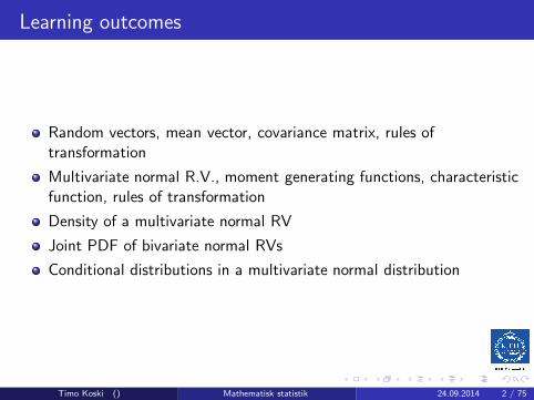
Learning outcomes
Random vectors, mean vector, covariance matrix, rules oftransformation
Multivariate normal R.V., moment generating functions, characteristicfunction, rules of transformation
Density of a multivariate normal RV
Joint PDF of bivariate normal RVs
Conditional distributions in a multivariate normal distribution
Timo Koski () Mathematisk statistik 24.09.2014 2 / 75

PART 1: Mean vector, Covariance matrix, MGF,Characteristic function
Timo Koski () Mathematisk statistik 24.09.2014 3 / 75

Vector Notation: Random Vector
A random vector X is a column vector
X =
X1
X2...Xn
= (X1,X2, . . . ,Xn)T
Each Xi is a random variable.
Timo Koski () Mathematisk statistik 24.09.2014 4 / 75

Sample Value Random Vector
A column vector
x =
x1x2...xn
= (x1, x2, . . . , xn)T
We can think of xi is an outcome of Xi .
Timo Koski () Mathematisk statistik 24.09.2014 5 / 75
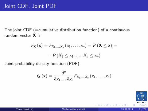
Joint CDF, Joint PDF
The joint CDF (=cumulative distribution function) of a continuousrandom vector X is
FX (x) = FX1,...,Xn(x1, . . . , xn) = P (X ≤ x) =
= P (X1 ≤ x1, . . . ,Xn ≤ xn)
Joint probability density function (PDF)
fX (x) =∂n
∂x1 . . . ∂xnFX1,...,Xn
(x1, . . . , xn)
Timo Koski () Mathematisk statistik 24.09.2014 6 / 75
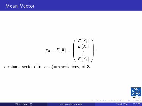
Mean Vector
µX = E [X] =
E [X1]E [X2]
...E [Xn]
,
a column vector of means (=expectations) of X.
Timo Koski () Mathematisk statistik 24.09.2014 7 / 75
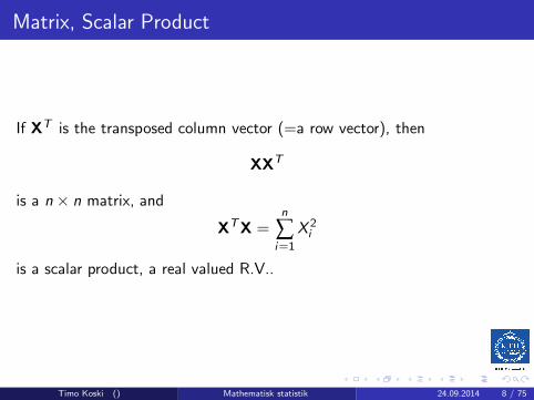
Matrix, Scalar Product
If XT is the transposed column vector (=a row vector), then
XXT
is a n× n matrix, and
XTX =n
∑i=1
X 2i
is a scalar product, a real valued R.V..
Timo Koski () Mathematisk statistik 24.09.2014 8 / 75
Covariance Matrix of A Random Vector
Covariance matrix
CX := E[
(X− µX) (X− µX)T]
where the element (i , j)
CX(i , j) = E [(Xi − µi ) (Xj − µj )]
is the covariance of Xi and Xj .
Timo Koski () Mathematisk statistik 24.09.2014 9 / 75
A Quadratic Form
xTCXx =n
∑i=1
n
∑j=1
xixjCX(i , j).
We see that
=n
∑i=1
n
∑j=1
xixjE [(Xi − µi ) (Xj − µj )]
= E
[n
∑i=1
n
∑j=1
xixj (Xi − µi ) (Xj − µj )
]
(∗)
Timo Koski () Mathematisk statistik 24.09.2014 10 / 75

Properties of a Covariance Matrix
Covariance matrix is nonnegative definite, i.e., for all x we have
xTCXx ≥ 0
HencedetCX ≥ 0.
The covariance matrix is symmetric
CX = CTX
Timo Koski () Mathematisk statistik 24.09.2014 11 / 75

Properties of a Covariance Matrix
The covariance matrix is symmetric
CX = CTX
sinceCX(i , j) = E [(Xi − µi ) (Xj − µj )]
= E [(Xj − µj ) (Xi − µi )] = CX(j , i)
Timo Koski () Mathematisk statistik 24.09.2014 12 / 75
Properties of a Covariance Matrix
A covariance matrix is positive definite,
xTCXx > 0
for all x 6= 0 iffdetCX > 0
(i.e. CX is invertible).
Timo Koski () Mathematisk statistik 24.09.2014 13 / 75
Properties of a Covariance Matrix
Proposition
xTCXx ≥ 0
Pf: By (∗) above
xTCXx = xTE[
(X− µX) (X− µX)T]
x
= E[
xT (X− µX) (X− µX)T x]
= E[
xTw ·wT x]
where we have set w = (X− µX). Then by linear algebra xTw = wTx= ∑
ni=1 wixi . Hence
E[
xTwwTx]
= E
(n
∑i=1
wixi
)2
≥ 0.
Timo Koski () Mathematisk statistik 24.09.2014 14 / 75
Properties of a Covariance Matrix
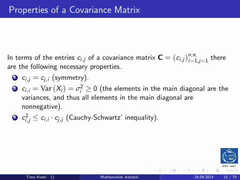
In terms of the entries ci ,j of a covariance matrix C = (ci ,j )n,n,i=1,j=1 there
are the following necessary properties.
1 ci ,j = cj ,i (symmetry).
2 ci ,i = Var (Xi ) = σ2i ≥ 0 (the elements in the main diagonal are the
variances, and thus all elements in the main diagonal arenonnegative).
3 c2i ,j ≤ ci ,i · cj ,j (Cauchy-Schwartz’ inequality).
Timo Koski () Mathematisk statistik 24.09.2014 15 / 75

Coefficient of Correlation
The Coefficient of Correlation ρ of X and Y is defined as
ρ := ρX ,Y :=Cov(X ,Y )
√
Var(X ) ·Var(Y ),
where Cov(X ,Y ) = E [(X − µX ) (Y − µY )]. This is normalized
−1 ≤ ρX ,Y ≤ 1
For random variables X and Y ,
Cov(X ,Y ) = ρX ,Y = 0 does not always mean that X ,Y areindependent.
Timo Koski () Mathematisk statistik 24.09.2014 16 / 75

Special case: Covariance Matrix of A Bivariate Vector
X = (X1,X2)T .
CX =
(σ21 ρσ1σ2
ρσ1σ2 σ22
)
,
where ρ is the coefficient of correlation of X1 and X2, and σ21 = Var (X1),
σ22 = Var (X2). CX is invertible iff ρ2 6= 1, for proof we note that
detCX = σ21σ2
2
(1− ρ2
)
Timo Koski () Mathematisk statistik 24.09.2014 17 / 75

Special case: Covariance Matrix of A Bivariate Vector
Λ =
(σ21 ρσ1σ2
ρσ1σ2 σ22
)
,
if ρ2 6= 1, the inverse exists and
Λ−1 =1
σ21σ2
2 (1− ρ2)
(σ22 −ρσ1σ2
−ρσ1σ2 σ21
)
,
Timo Koski () Mathematisk statistik 24.09.2014 18 / 75
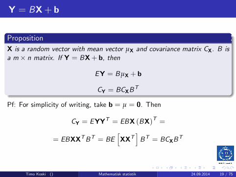
Y = BX+ b
Proposition
X is a random vector with mean vector µX and covariance matrix CX. B is
a m× n matrix. If Y = BX+ b, then
EY = BµX + b
CY = BCXBT
Pf: For simplicity of writing, take b = µ = 0. Then
CY = EYYT = EBX (BX)T =
= EBXXTBT = BE[
XXT]
BT = BCXBT
Timo Koski () Mathematisk statistik 24.09.2014 19 / 75

Moment Generating and Characteristic Functions
Definition
Moment generating function of X is defined as
ψX (t)def= Eet
TX = Eet1X1+t2X2+···+tnXn
Definition
Characteristic function of X is defined as
ϕX (t)def= Ee it
TX = Ee i (t1X1+t2X2+···+tnXn)
Special cases: take t1 = 1, t2 = t3 = . . . = tn = 0, thenϕX (t) = ϕX1 (t1).
Timo Koski () Mathematisk statistik 24.09.2014 20 / 75

PART 2: Def I of a multivariate normal distribution
We recall first some of the properties of univariate normal distribution
Timo Koski () Mathematisk statistik 24.09.2014 21 / 75

Normal (Gaussian) One-dimensional RVs
X is a normal random variable if
fX (x) =1
σ√2π
e− 1
2σ2(x−µ)2
where µ is real and σ > 0.
Notation: X ∈ N(µ, σ2)
Properties: E (X ) = µ, Var = σ2
Timo Koski () Mathematisk statistik 24.09.2014 22 / 75
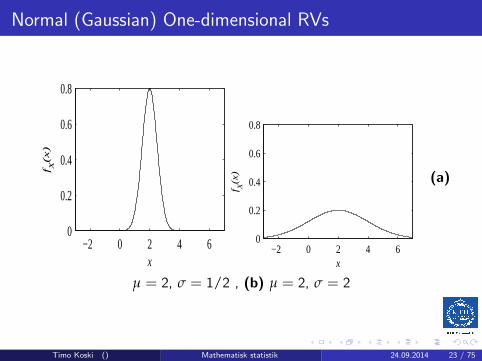
Normal (Gaussian) One-dimensional RVs
−2 0 2 4 60
0.2
0.4
0.6
0.8
x
f X(x
)
−2 0 2 4 60
0.2
0.4
0.6
0.8
x
f X(x
) (a)
µ = 2, σ = 1/2 , (b) µ = 2, σ = 2
Timo Koski () Mathematisk statistik 24.09.2014 23 / 75

Linear Transformation
X ∈ N(µX , σ2) ⇒ Y = aX + b is N(aµX + b, a2σ2)
Thus Z = X−µX
σX∈ N(0, 1) and
P(X ≤ x) = P
(X − µX
σX≤ x − µX
σX
)
or
FX (x) = P
(
Z ≤ x − µX
σX
)
= Φ
(x − µX
σX
)
Timo Koski () Mathematisk statistik 24.09.2014 24 / 75
Normal (Gaussian) One-dimensional RVs
X ∈ N(µ, σ2) then the moment generating function is
ψX (t) = E[
etX]
= etµ+ 12 t
2σ2,
and the characteristic function is
ϕX (t) = E[
e itX]
= e itµ− 12 t
2σ2
as found in previous Lectures.
Timo Koski () Mathematisk statistik 24.09.2014 25 / 75

Multivariate Normal Def. I
Definition
An n× 1 random vector X has a normal distribution iff for every
n× 1-vector a the one-dimensional random vector aTX has a normal
distribution.
We write X ∈ N (µ,Λ), when µ is the mean vector and Λ is thecovariance matrix.
Timo Koski () Mathematisk statistik 24.09.2014 26 / 75
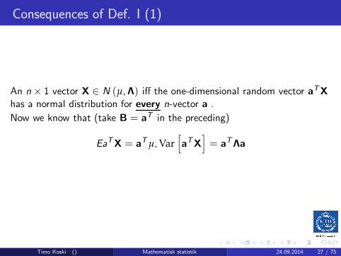
Consequences of Def. I (1)
An n× 1 vector X ∈ N (µ,Λ) iff the one-dimensional random vector aTXhas a normal distribution for every n-vector a .
Now we know that (take B = aT in the preceding)
EaTX = aTµ,Var[
aTX]
= aTΛa
Timo Koski () Mathematisk statistik 24.09.2014 27 / 75

Consequences of Def. I (2)
Hence, if Y = aTX, then Y ∈ N(aTµ, aTΛa
)and the moment
generating function of Y is
ψY (t) = E[
etY]
= etaT µ+ 1
2 t2aTΛa.
ThereforeψX (a) = Eea
TX = ψY (1) = eaT µ+ 1
2aTΛa.
Timo Koski () Mathematisk statistik 24.09.2014 28 / 75

Consequences of Def. I (3)
Hence we have shown that if X ∈ N (µ,Λ), then
ψX (t) = EetTX = et
T µ+ 12 t
TΛt.
is the moment generating function of X.
Timo Koski () Mathematisk statistik 24.09.2014 29 / 75

Consequences of Def. I (4)
In the same way we can find that
ϕX (t) = Ee itTX = e it
T µ− 12 t
TΛt.
is the characteristic function of X ∈ N (µ,Λ).
Timo Koski () Mathematisk statistik 24.09.2014 30 / 75
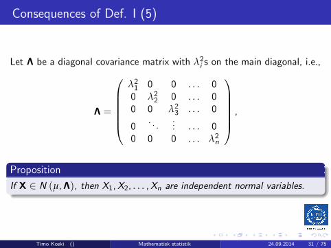
Consequences of Def. I (5)
Let Λ be a diagonal covariance matrix with λ2i s on the main diagonal, i.e.,
Λ =
λ21 0 0 . . . 00 λ2
2 0 . . . 00 0 λ2
3 . . . 0
0. . .
... . . . 00 0 0 . . . λ2
n
,
Proposition
If X ∈ N (µ,Λ), then X1,X2, . . . ,Xn are independent normal variables.
Timo Koski () Mathematisk statistik 24.09.2014 31 / 75
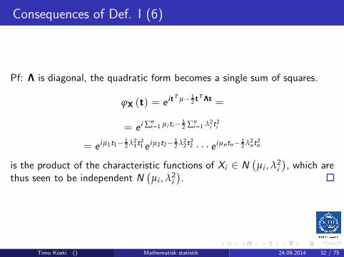
Consequences of Def. I (6)
Pf: Λ is diagonal, the quadratic form becomes a single sum of squares.
ϕX (t) = e itT µ− 1
2 tTΛt =
= e i ∑ni=1 µi ti− 1
2 ∑ni=1 λ2
i t2i
= e iµ1t1− 12 λ2
1t21 e iµ2t2− 1
2 λ22t
22 · · · e iµntn− 1
2 λ2nt
2n
is the product of the characteristic functions of Xi ∈ N(µi ,λ2
i
), which are
thus seen to be independent N(µi ,λ2
i
).
Timo Koski () Mathematisk statistik 24.09.2014 32 / 75
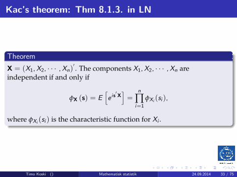
Kac’s theorem: Thm 8.1.3. in LN
Theorem
X = (X1,X2, · · · ,Xn)′. The components X1,X2, · · · ,Xn are
independent if and only if
φX (s) = E[
e is′X]
=n
∏i=1
φXi(si ),
where φXi(si ) is the characteristic function for Xi .
Timo Koski () Mathematisk statistik 24.09.2014 33 / 75

Further properties of the multivariate normal
X ∈ N (µ,Λ)
Every component Xk is one-dimensional normal. To prove this we take
a = (0, 0, . . . , 1︸︷︷︸
position k
, 0, . . . , 0)T
and the conclusion follows by Def. I.
X1 + X2 + · · ·Xn is one-dimensional normal. Note: The terms in thesum need not be independent.
Timo Koski () Mathematisk statistik 24.09.2014 34 / 75

Properties of multivariate normal
X ∈ N (µ,Λ)
Every marginal distribution of k variables ( 1 ≤ k < n is normal. Toprove this we consider any k variables Xi1 ,Xi2 . . .Xik and then take asuch that aj = 0 for j 6= i1, . . . ik and then apply Def. I.
Timo Koski () Mathematisk statistik 24.09.2014 35 / 75
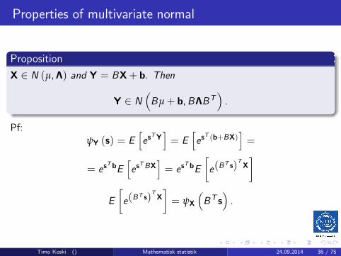
Properties of multivariate normal
Proposition
X ∈ N (µ,Λ) and Y = BX+ b. Then
Y ∈ N(
Bµ + b,BΛBT)
.
Pf:ψY (s) = E
[
esTY]
= E[
esT (b+BX)
]
=
= esT bE
[
esTBX
]
= esT bE
[
e(BT s)
TX
]
E
[
e(BT s)
TX
]
= ψX
(
BT s)
.
Timo Koski () Mathematisk statistik 24.09.2014 36 / 75
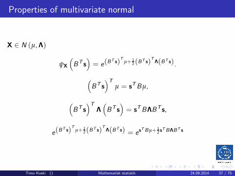
Properties of multivariate normal
X ∈ N (µ,Λ)
ψX
(
BT s)
= e(BT s)
Tµ+ 1
2 (BT s)TΛ(BT s).
(
BT s)T
µ = sTBµ,
(
BT s)T
Λ(
BT s)
= sTBΛBTs,
e(BT s)
Tµ+ 1
2(BT s)TΛ(BT s) = es
TBµ+ 12 s
TBΛBT s
Timo Koski () Mathematisk statistik 24.09.2014 37 / 75
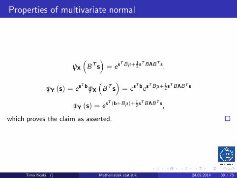
Properties of multivariate normal
ψX
(
BT s)
= esTBµ+ 1
2 sTBΛBT s.
ψY (s) = esTbψX
(
BT s)
= esTbes
TBµ+ 12 s
TBΛBT s
ψY (s) = esT (b+Bµ)+ 1
2 sTBΛBT s,
which proves the claim as asserted.
Timo Koski () Mathematisk statistik 24.09.2014 38 / 75
PART 3: Multivariate normal, Def. II: characteristic
function, DEF III: density
Timo Koski () Mathematisk statistik 24.09.2014 39 / 75

Multivariate normal, Def. II: char. fnctn
Definition
A random vector X with mean vector µ and a covariance matrix Λ is
N (µ,Λ) if its characteristic function is
ϕX (t) = Ee itTX = e it
T µ− 12 t
TΛt.
Timo Koski () Mathematisk statistik 24.09.2014 40 / 75

Multivariate normal, Def. II implies Def. I
We need to show that the one-dimensional random vector Y = aTX has anormal distribution.
ϕY (t) = E[
e itY]
= E[
e it ∑ni=1 ai ·Xi
]
=
= E[
e itaTX]
= ϕX (ta) =
= e itaT µ− 1
2 t2aTΛa
and this is the characteristic function of N(aTµ, aTΛa
).
Timo Koski () Mathematisk statistik 24.09.2014 41 / 75
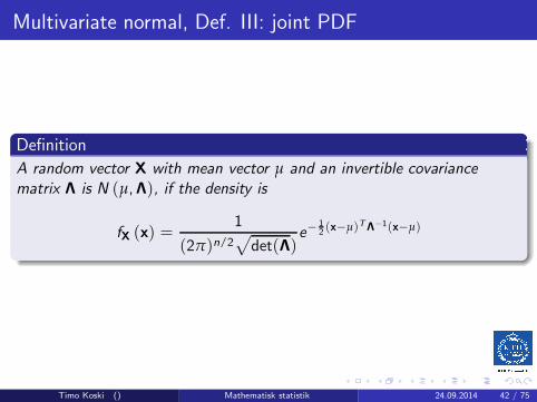
Multivariate normal, Def. III: joint PDF
Definition
A random vector X with mean vector µ and an invertible covariance
matrix Λ is N (µ,Λ), if the density is
fX (x) =1
(2π)n/2√
det(Λ)e−
12 (x−µ)TΛ−1(x−µ)
Timo Koski () Mathematisk statistik 24.09.2014 42 / 75
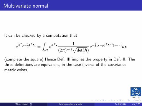
Multivariate normal
It can be checked by a computation that
e itT µ− 1
2 tTΛt =
∫
Rne it
T x 1
(2π)n/2√
det(Λ)e−
12 (x−µ)TΛ−1(x−µ)dx
(complete the square) Hence Def. III implies the property in Def. II. Thethree definitions are equivalent, in the case inverse of the covariancematrix exists.
Timo Koski () Mathematisk statistik 24.09.2014 43 / 75

PART 4: Bivariate normal with density
Timo Koski () Mathematisk statistik 24.09.2014 44 / 75
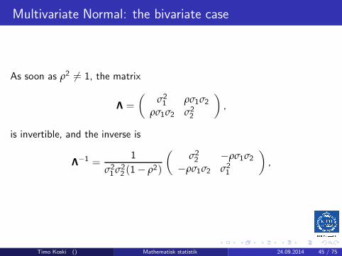
Multivariate Normal: the bivariate case
As soon as ρ2 6= 1, the matrix
Λ =
(σ21 ρσ1σ2
ρσ1σ2 σ22
)
,
is invertible, and the inverse is
Λ−1 =1
σ21σ2
2 (1− ρ2)
(σ22 −ρσ1σ2
−ρσ1σ2 σ21
)
,
Timo Koski () Mathematisk statistik 24.09.2014 45 / 75
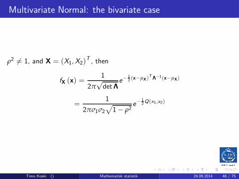
Multivariate Normal: the bivariate case
ρ2 6= 1, and X = (X1,X2)T , then
fX (x) =1
2π√detΛ
e−12 (x−µX)
TΛ−1(x−µX)
=1
2πσ1σ2√
1− ρ2e−
12Q(x1,x2)
Timo Koski () Mathematisk statistik 24.09.2014 46 / 75

Multivariate Normal: the bivariate case
whereQ(x1, x2) =
1
(1− ρ2)·[(
x1 − µ1
σ1
)2
− 2ρ(x1 − µ1)(x2 − µ2)
σ1σ2+
(x2 − µ2
σ2
)2]
For this, invert the matrix Λ and expand the quadratic form !
Timo Koski () Mathematisk statistik 24.09.2014 47 / 75

ρ = 0
0
0.35
0.3
0.25
0.2
0.15
0.1
0.05
0
0
32
10
-1-2
-3
0
3
2
1
0
-1
-2
-3
Timo Koski () Mathematisk statistik 24.09.2014 48 / 75

ρ = 0.9
0
0.35
0.3
0.25
0.2
0.15
0.1
0.05
0
0
32
10
-1-2
-3
0
3
2
1
0
-1
-2
-3
Timo Koski () Mathematisk statistik 24.09.2014 49 / 75
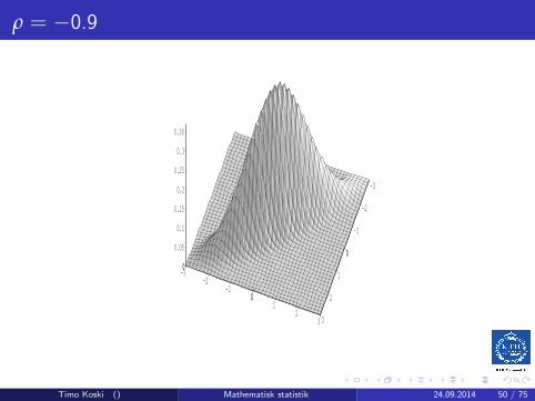
ρ = −0.9
0
0.35
0.3
0.25
0.2
0.15
0.1
0.05
0
0
32
10
-1-2
-3
0
3
2
1
0
-1
-2
-3
Timo Koski () Mathematisk statistik 24.09.2014 50 / 75
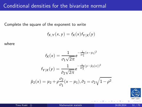
Conditional densities for the bivariate normal
Complete the square of the exponent to write
fX ,Y (x , y ) = fX (x)fY |X (y )
where
fX (x) =1
σ1√2π
e− 1
2σ21(x−µ1)2
fY |X (y ) =1
σ̃2√2π
e− 1
2σ̃22(y−µ̃2(x))2
µ̃2(x) = µ2 + ρσ2σ1
(x − µ1), σ̃2 = σ2
√
1− ρ2
Timo Koski () Mathematisk statistik 24.09.2014 51 / 75

Bivariate normal properties
E (X ) = µ1
Given X = x , Y is Gaussian
Conditional mean of Y given X = x :
µ̃2(x) = µ2 + ρσ2σ1
(x − µ1) = E (Y |X = x)
Conditional variance of Y given X = x :
Var(Y |X = x) = σ22
(1− ρ2
)
Timo Koski () Mathematisk statistik 24.09.2014 52 / 75
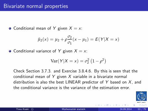
Bivariate normal properties
Conditional mean of Y given X = x :
µ̃2(x) = µ2 + ρσ2σ1
(x − µ1) = E (Y |X = x)
Conditional variance of Y given X = x :
Var(Y |X = x) = σ22
(1− ρ2
)
Check Section 3.7.3. and Exercise 3.8.4.6. By this is seen that theconditional mean of Y given X variable in a bivariate normaldistribution is also the best LINEAR predictor of Y based on X , andthe conditional variance is the variance of the estimation error.
Timo Koski () Mathematisk statistik 24.09.2014 53 / 75

Marginal PDFs
Timo Koski () Mathematisk statistik 24.09.2014 54 / 75
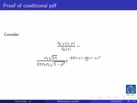
Proof of conditional pdf
Consider
fX ,Y (x , y )
fX (x)=
σ1√2π
2πσ1σ2√
1− ρ2e− 1
2Q(x ,y )+ 1
2σ21(x−µ1)2
Timo Koski () Mathematisk statistik 24.09.2014 55 / 75

Proof of conditional pdf
−1
2Q(x , y ) +
1
2σ21
(x − µ1)2
= −1
2H(x , y ),
Timo Koski () Mathematisk statistik 24.09.2014 56 / 75
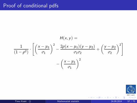
Proof of conditional pdfs
H(x , y ) =
1
(1− ρ2)·[(
x − µ1
σ1
)2
− 2ρ(x − µ1)(y − µ2)
σ1σ2+
(y − µ2
σ2
)2]
−(x − µ1
σ1
)2
Timo Koski () Mathematisk statistik 24.09.2014 57 / 75

Proof of conditional pdf
H(x , y ) =
ρ2
(1− ρ2)
(x − µ1)2
σ21
− 2ρ(x − µ1)(y − µ2)
σ1σ2(1− ρ2)+
(y − µ2)2
σ22 (1− ρ2)
Timo Koski () Mathematisk statistik 24.09.2014 58 / 75
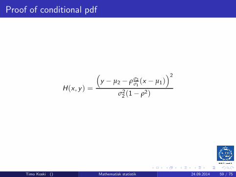
Proof of conditional pdf
H(x , y ) =
(
y − µ2 − ρ σ2σ1(x − µ1)
)2
σ22 (1− ρ2)
Timo Koski () Mathematisk statistik 24.09.2014 59 / 75

Conditional pdf
fX ,Y (x , y )
fX (x)=
1√
1− ρ2σ2√2π
e
− 12
(y−µ2−ρσ2σ1
(x−µ1))2
σ22 (1−ρ2)
This establishes the bivariate normal properties claimed above.
Timo Koski () Mathematisk statistik 24.09.2014 60 / 75

Bivariate normal properties : ρ
Proposition
(X ,Y ) bivariate normal ⇒ ρ = ρX ,Y
Proof:
E [(X − µ1)(Y − µ2)]
= E (E ([(X − µ1)(Y − µ2)] |X ))
= E ((X − µ1)E [Y − µ2] |X ))
Timo Koski () Mathematisk statistik 24.09.2014 61 / 75
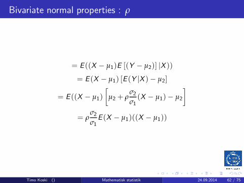
Bivariate normal properties : ρ
= E ((X − µ1)E [(Y − µ2)] |X ))
= E (X − µ1) [E (Y |X )− µ2]
= E ((X − µ1)
[
µ2 + ρσ2σ1
(X − µ1)− µ2
]
= ρσ2σ1
E (X − µ1)((X − µ1))
Timo Koski () Mathematisk statistik 24.09.2014 62 / 75
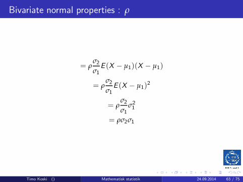
Bivariate normal properties : ρ
= ρσ2σ1
E (X − µ1)(X − µ1)
= ρσ2σ1
E (X − µ1)2
= ρσ2σ1
σ21
= ρσ2σ1
Timo Koski () Mathematisk statistik 24.09.2014 63 / 75

Bivariate normal properties : ρ
In other words we have checked that
ρ =E [(X − µ1)(Y − µ2)]
σ2σ1
ρ = 0 ⇔ bivariate normal X ,Y are independent.
Timo Koski () Mathematisk statistik 24.09.2014 64 / 75

PART 5: Generating a multivariate normal variable
Timo Koski () Mathematisk statistik 24.09.2014 65 / 75
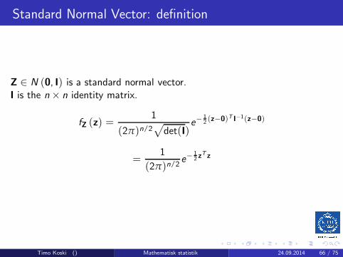
Standard Normal Vector: definition
Z ∈ N (0, I) is a standard normal vector.I is the n× n identity matrix.
fZ (z) =1
(2π)n/2√
det(I)e−
12 (z−0)T I−1(z−0)
=1
(2π)n/2e−
12 z
T z
Timo Koski () Mathematisk statistik 24.09.2014 66 / 75

Distribution of X = AZ+ b
X = AZ+ b, Z is standard Gaussian, then
X = N(
b,AAT)
(follows by a rule in the preceding)
Timo Koski () Mathematisk statistik 24.09.2014 67 / 75
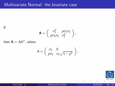
Multivariate Normal: the bivariate case
If
Λ =
(σ21 ρσ1σ2
ρσ1σ2 σ22
)
,
then Λ = AAT , where
A =
(σ1 0
ρσ2 σ2√
1− ρ2
)
,
Timo Koski () Mathematisk statistik 24.09.2014 68 / 75
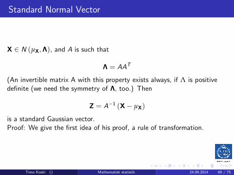
Standard Normal Vector
X ∈ N (µX,Λ), and A is such that
Λ = AAT
(An invertible matrix A with this property exists always, if Λ is positivedefinite (we need the symmetry of Λ, too.) Then
Z = A−1 (X− µX)
is a standard Gaussian vector.Proof: We give the first idea of his proof, a rule of transformation.
Timo Koski () Mathematisk statistik 24.09.2014 69 / 75
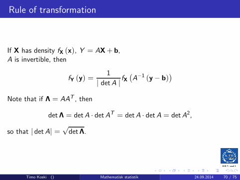
Rule of transformation
If X has density fX (x), Y = AX+ b,A is invertible, then
fY (y) =1
| detA | fX(A−1 (y− b)
)
Note that if Λ = AAT , then
detΛ = detA · detAT = detA · detA = detA2,
so that | detA| =√detΛ.
Timo Koski () Mathematisk statistik 24.09.2014 70 / 75

Johann Carl Friedrich Gauss (30 April 1777 23 February
1855)
Timo Koski () Mathematisk statistik 24.09.2014 71 / 75

Diagonalizable Matrices
An n× n matrix A is orthogonally diagonalizable, if there is anorthogonal matrix P (i.e., PTP =PPT = I) such that
PTAP = Λ,
where Λ is a diagonal matrix.
Timo Koski () Mathematisk statistik 24.09.2014 72 / 75
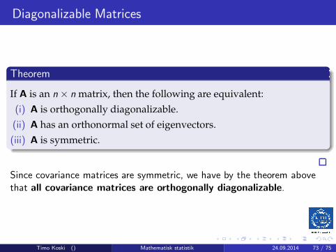
Diagonalizable Matrices
Theorem
If A is an n× n matrix, then the following are equivalent:
(i) A is orthogonally diagonalizable.
(ii) A has an orthonormal set of eigenvectors.
(iii) A is symmetric.
Since covariance matrices are symmetric, we have by the theorem abovethat all covariance matrices are orthogonally diagonalizable.
Timo Koski () Mathematisk statistik 24.09.2014 73 / 75

Diagonalizable Matrices
Theorem
If A is a symmetric matrix, then
(i) Eigenvalues of A are all real numbers.
(ii) Eigenvectors from different eigenspaces are orthogonal.
That is, all eigenvalues of a covariance matrix are real.
Timo Koski () Mathematisk statistik 24.09.2014 74 / 75
Diagonalizable Matrices
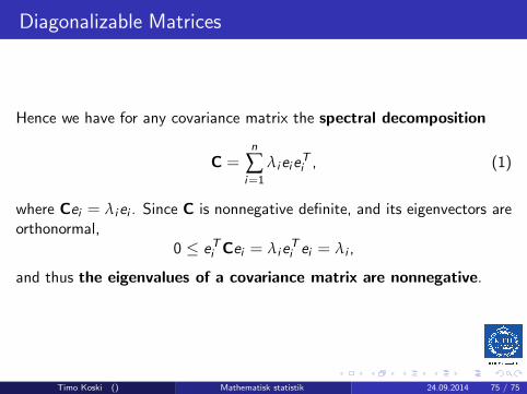
Hence we have for any covariance matrix the spectral decomposition
C =n
∑i=1
λieieTi , (1)
where Cei = λiei . Since C is nonnegative definite, and its eigenvectors areorthonormal,
0 ≤ eTi Cei = λieTi ei = λi ,
and thus the eigenvalues of a covariance matrix are nonnegative.
Timo Koski () Mathematisk statistik 24.09.2014 75 / 75
Diagonalizable Matrices
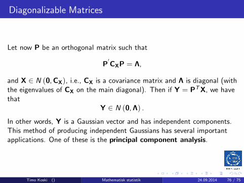
Let now P be an orthogonal matrix such that
P′CXP = Λ,
and X ∈ N (0,CX), i.e., CX is a covariance matrix and Λ is diagonal (withthe eigenvalues of CX on the main diagonal). Then if Y = PTX, we havethat
Y ∈ N (0,Λ) .
In other words, Y is a Gaussian vector and has independent components.This method of producing independent Gaussians has several importantapplications. One of these is the principal component analysis.
Timo Koski () Mathematisk statistik 24.09.2014 76 / 75


