Page 1
1
Mathematical Modelling and Control of Renewable
Energy Systems and Battery Storage Systems
A thesis submitted by
Singappuli M Wijewardana
in partial fulfilment of
the requirements of the degree of
Doctor of Philosophy
School of Engineering and Materials Science
Queen Mary, University of London
Mile End Road
London, E1 4NS, UK
October 2016
Page 2
2
School of Engineering and Materials Science
Queen Mary, University of London
PhD THESIS
DECLARATION
this thesis entitled
Mathematical Modelling and Control of
Renewable Energy Systems and Battery Storage
Systems
presented herewith is my own work and this thesis has not been submitted for any
other qualifications.
Signed
Name: SINGAPPULI M WIJEWARDANA
Date: 12 October 2016
Page 3
3
Abstract
Intermittent nature of renewable energy sources like the wind and solar energy poses new
challenges to harness and supply uninterrupted power for consumer usage. Though, converting
energy from these sources to useful forms of energy like electricity seems to be promising, still,
significant innovations are needed in design and construction of wind turbines and PV arrays
with BS systems. The main focus of this research project is mathematical modelling and control
of wind turbines, solar photovoltaic (PV) arrays and battery storage (BS) systems. After careful
literature review on renewable energy systems, new developments and existing modelling and
controlling methods have been analysed. Wind turbine (WT) generator speed control, turbine
blade pitch angle control (pitching), harnessing maximum power from the wind turbines have
been investigated and presented in detail. Mathematical modelling of PV arrays and how to
extract maximum power from PV systems have been analysed in detail.
Application of model predictive control (MPC) to regulate the output power of the wind turbine
and generator speed control with variable wind speeds have been proposed by formulating a
linear model from a nonlinear mathematical model of a WT.
Battery chemistry and nonlinear behaviour of battery parameters have been analysed to present
a new equivalent electrical circuit model. Converting the captured solar energy into useful
forms, and storing it for future use when the Sun itself is obscured is implemented by using
battery storage systems presenting a new simulation model.
Temperature effect on battery cells and dynamic battery pack modelling have been described
with an accurate state of charge estimation method. The concise description on power
converters is also addressed with special reference to state-space models. Bi-directional
AC/DC converter, which could work in either rectifier or inverter modes is described with a
cost effective proportional integral derivative (PID/State-feedback) controller.
Page 4
4
Preface
This dissertation is original, prepared by Singappuli Wijewardana at the School of Engineering
and Materials Science, Queen Mary, University of London, Mile End Road, London E1 4NS,
UK in partial fulfilment of the degree of Doctor of Philosophy in Engineering. The research
project has been supervised by Dr Hasan Shaheed.
This interdisciplinary research project has a potential for substantial impact on multiple
renewable energy electricity generations from WT, PV combined with BS systems. With this
compendium, I have attempted to bring everything in concise and conscientious manner.
With the mathematical modelling and simulation for every renewable energy subsystem under
consideration, model predictive control (MPC) is applied to the wind turbine control and
optimising power output. MATLAB/Simulink has been used as a tool for modelling and
simulations.
Singappuli M Wijewardana 12 October 2016
Page 5
5
Acknowledgement
I wish to express my profound thanks and deepest gratitude towards my supervisor Dr M Hasan
Shaheed for his invaluable guidance and support during my research project. He guided me in
every aspect during my studies and encouraged me at every stage when I had questions
regarding my project. Also, I wish to thank Dr Ranjan Vepa for his valuable advice given to
me during my research work.
I dedicate this thesis to Professor Sam Karunaratne, former Chairman and Chancellor, SLIIT
and Vice Chancellor University of Moratuwa, Sri Lanka. Without his blessings and advice at
the inception, I would not have embarked on this research endeavour.
I owe my sincere thanks to my wife Sujatha and I am indebted to her for her patience and
encouragement. Ishan, Ishanga my son and daughter, have been always helpful to me in
numerous ways during my research work. Finally, I would like to thank my mother for giving
me the moral support that I needed to complete this task.
Singappuli M Wijewardana
12 October 2016
Page 6
6
Table of Contents
Title Page 1
Abstract 3
Preface 4
Acknowledgement 5
Table of Contents 6
List of Figures 8
List of Tables 11
Acronyms & Symbols 11
Chapter 1 Introduction 17
1.1 Background 17 1.2 Mathematical Modelling and Control of WT, PV Arrays
& BS Systems 18
1.3 Literature Review and Recent Developments 19 1.4 Motivation 42 1.5 Aims and Objectives 43 1.6 Contribution 45 1.7 Outline of the Thesis 46 1.8 Journal Publications 47 Chapter 2 Dynamic Battery Cell Modelling and State of Charge
Estimation with Temperature Effects.
48
2.0 Introduction 48 2.1 Introduction to Dynamic Battery Cell Modelling 49 2.2 Thermal Effect on the Battery Cell Modelling 55 2.3 Battery Pack Modelling 63 2.4 Mathematical Formulations for the Battery Pack
Modelling 64
2.5 Experimental Validation of the BP Model 72 2.6 The state-space Model 73 2.7 Kalman Filter Application to Battery Cell Model 75 2.8 Kalman Filter in Simulink 76 2.9 Conclusion 81 Chapter 3 Nonlinear Modelling and Feedback Control of Variable
Speed Wind Turbines
83
3.0 Introduction 83 3.1 Mathematical Modelling and Simulations 84 3.2 Wind Model 91 3.3 MPPT from the Wind Turbine 93 3.4 Modelling Wind Turbine Subsystems 101 3.5 Generator-side Modelling 126 3.6 Doubly Fed Induction Generator 127 3.7 Generator Modelling and Reference frames 130 Chapter 4 Model Predictive Control 137
4.0 Introduction 137
Page 7
7
4.1 Advantages and disadvantages of PID control, MPC and Gain Scheduling
139
4.2 Analytical Approach to MPC Designs 141 4.3 Wind regions 146 4.4 Application of MPC for WT Control 148 4.5 Optimum Power Output Control of Wind Turbine Rotor 152 4.6 Blade Element Momentum Theory for Power Coefficient 152 4.7 Dynamic Stall Modelling 153 4.8 Application to Power Output Regulation 154 4.9 Analysis of the Results 160 Chapter 5 Power Converters 163
5.0 Introduction 163 5.1 Pulse Width Modulation (PWM) 165 5.2 Grid-Side Converter Modelling 169 5.3 Rotor-Side Converter Modelling 172 5.4 Dynamic Modelling of Synchronous Buck Converter 174 5.5 Power converter applications 184 Chapter 6 Dynamic Modelling of SPV Cells 187
6.0 Introduction 187 6.1 Dynamic Modelling of PV Cells 189 6.2 Simulation Results of the Dynamic PV Cell Model 191 6.3 Maximum Power Point Tracking (MPPT) 194 Chapter 7 Conclusions and suggestion for future work 196
7.0 Conclusions 196 7.1 Suggestions for future work 197 Appendix A Output measurement noise and Augmented Model 201 A MATLAB Program Codes 204 A MATLAB Script for PC _max Calculation 205 A MATLAB Functions for WT MPC Control 206 B Computing Toeplitz Matrix φ From MATLAB 223 B Script File for Bode Plot. 224 B MATLAB Script files for PV Cells and Arrays 224 B Dynamic PV Cell Model in Simulink 228 C Discretization of continuous time state space models 229 C Kalman Filter 230 C Covariance Matrix 233 D Introduction to Linearization via Taylor Series
Expansion 236
E Permission letters from Reputed Authors 239 Bibliography References 243 END 262
Page 8
8
List of Figures
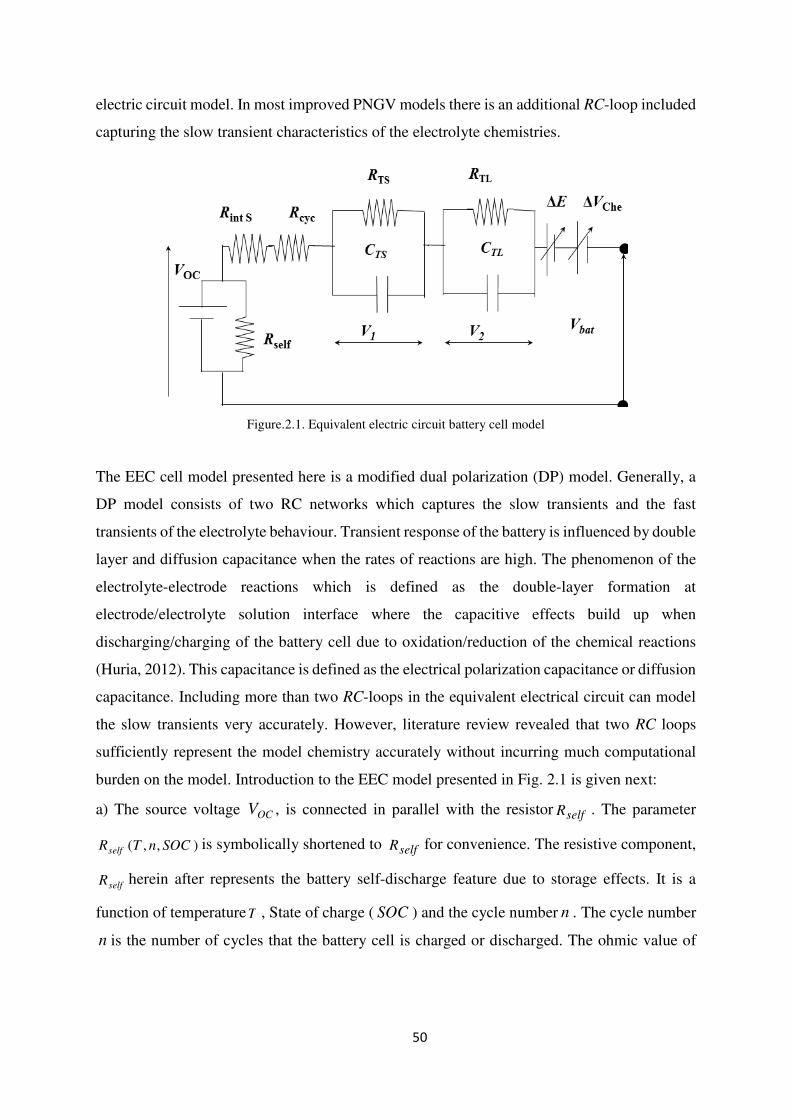
2.1 Equivalent electrical battery cell model. 49
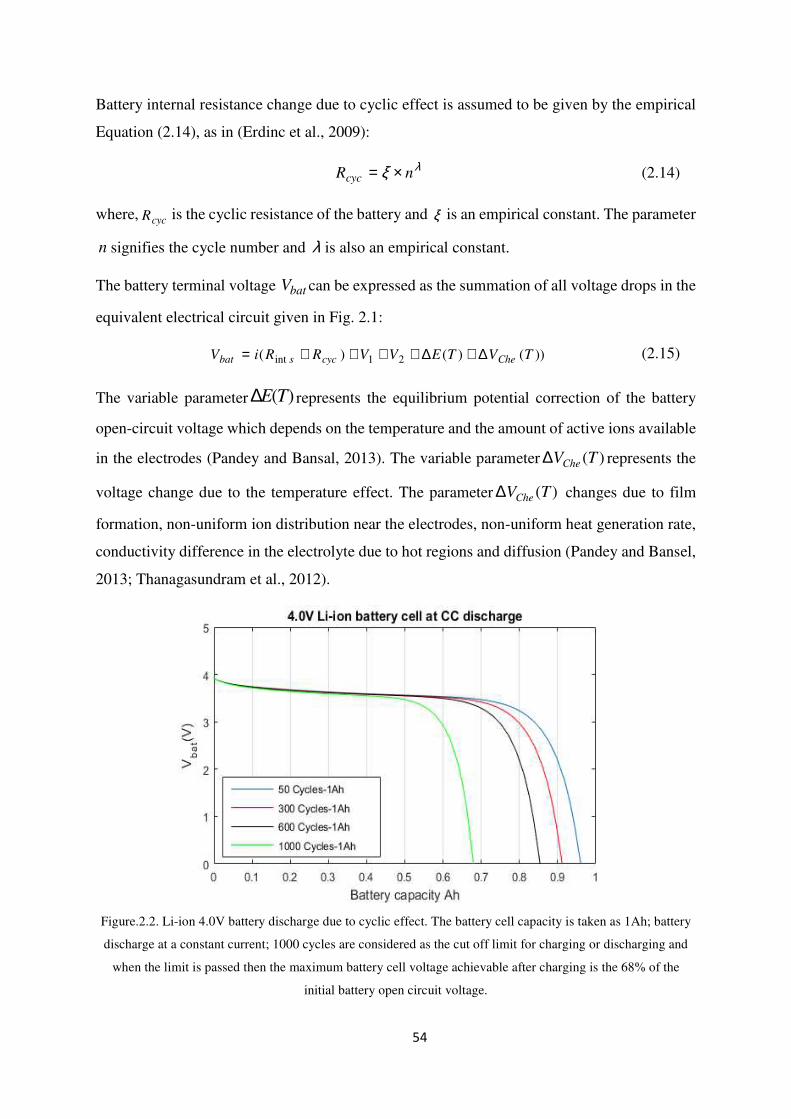
2.2 Li-ion 4.0V battery discharge due to cyclic effect. 53
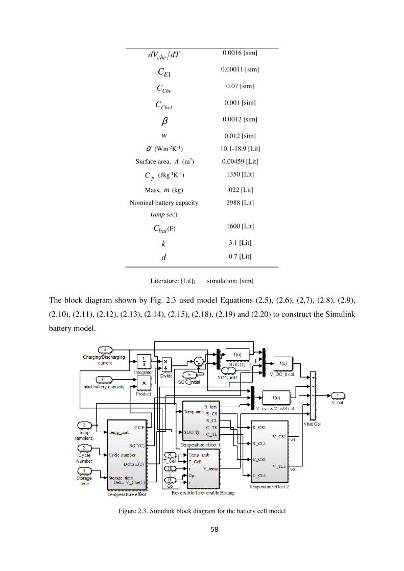
2.3 Simulink block diagram for the battery cell model. 57
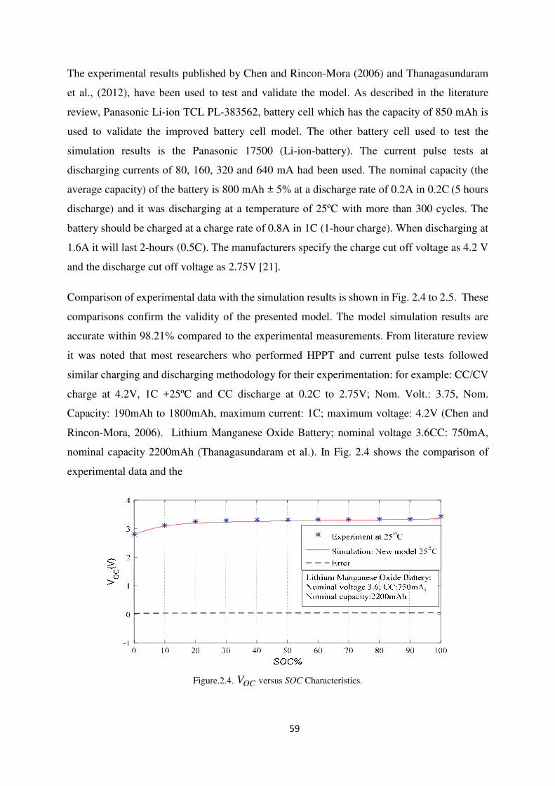
2.4 OCV versus SOC Characteristics. 58
2.5 OCV versus SOC Characteristics. 59
2.6 TLR versus SOC Characteristics. 59
2.7 TSC versus SOC Characteristics. 60
2.8 OCV versus discharge capacity at different temperatures. 61
2.9 OCV versus discharge capacity at different temperatures
(Manufacturer’s data).
61
2.10 batV versus discharge capacity at different temperatures. 62
2.11 Improved simulation results model based on Saiju et al. (2008), cell model
63
2.12 The SIMULINK block diagram of two cells CellMaxVN × ,( 2=N )
connected in series.
64
2.13 Simulink block diagram of two cells in parallel. 64
2.14.a a) The Simulink block diagram of three 12V batteries ( 3=N ) connected in series. b) the characteristics of batV versus the simulation time at 1C, 25ºC.
67
2.14.b three 12 V batteries in series: the simulation characteristics of batV
versus the simulation time at 1C, at 25ºC. 67
2.15.a The Simulink block diagram of three 12V batteries in parallel. 68
2.15.b The variation of Vbat versus the simulation time at 25ºC: Case A: three 12V batteries in parallel. Case B: two 12V batteries in parallel. Case C: single 12V battery simulation.
68
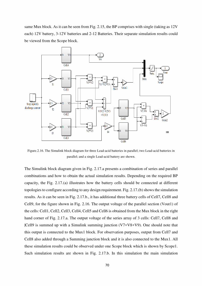
2.16 The Simulink block diagram for three Lead-acid batteries in parallel and two Lead-acid batteries in parallel and a single Lead-acid battery are shown.
69
2.17.a The SIMULINK block diagram of nine 12V Lead-acid batteries connected in different topologies
70
2.17.b Sectional simulations of battery output voltage versus simulation time in seconds at 25ºC.
70
2.18 Battery pack model comparison with experimental data published by Dubarry et al. (2009)
71
Page 9
9
2.19 Battery pack model comparison with experimental data published by Ganesan et al. (2016)
71
2.20 Modified equivalent battery circuit model for state-space applications.
72
2.21 Extended Kalman Filter for battery output voltage estimation: Equations (2.42) to (2.46) are modelled in Simulink: battery cell model considered as a plant in state-space.
77
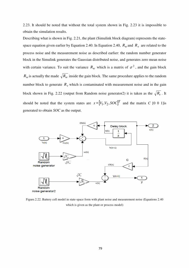
2.22 Battery cell model in state-space form with plant noise and measurement noise (Equations 2.40 which is given as the plant or process model)
78
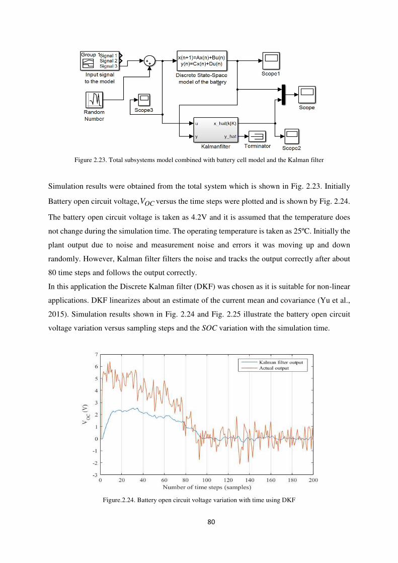
2.23 Total subsystems model combined with battery cell model and the Kalman filter
78
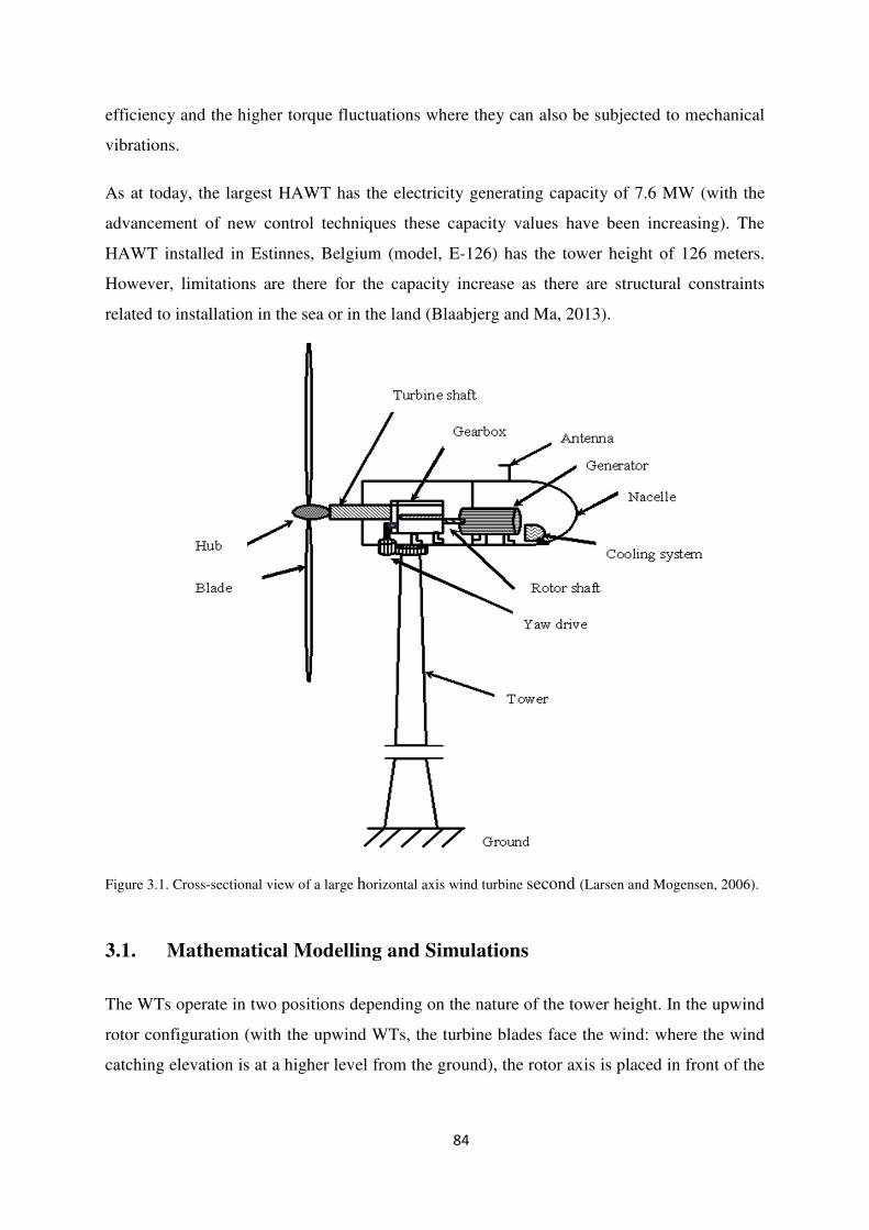
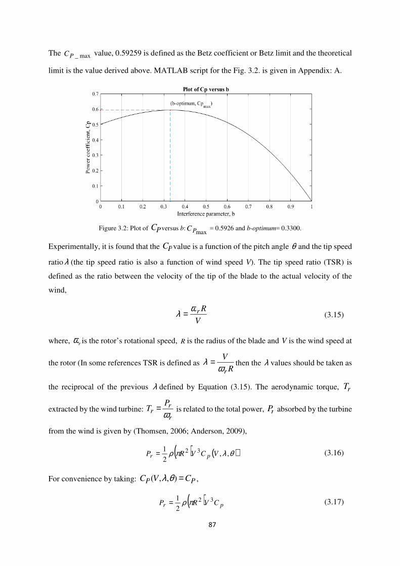
2.24 Battery open circuit voltage variation with time using DKF 79 2.25 Battery SOC estimation versus time using EKF 81 3.1 WT Cross-sectional view and its parts. 84 3.2 Plot of PC versus b: max_PC = 0.5926 and b-optimum= 0.3300. 86
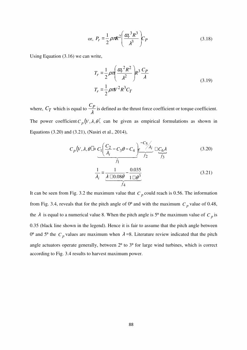
3.3 PC plot with varying θ and λ . 88
3.4 Characteristics of PC versus λ at constant temperature and varying the pitch angle.
88
3.5 Typical values of PC and TC versus λ at a constant pitch angle. 89
3.6 Simulink (Subsystems model) model for PC calculations. 89
3.7 Simulink model which calculates the PC versus λ with varying pitch angle θ at constant temperature.
90
3.8 Simulink Wind Model. 91 3.9 Wind speed variation with time: mean wind speed = 8m/s. 92
3.10 Pitch angle versus pC . 94
3.11 Block diagram for the Equation (3.36) (a, b, k: numerical constants).
98
3.12 Turbine rotor speed control block diagram: closed loop. 98 3.13 Modified pitch control and generator speed control with a new
wind model. 99
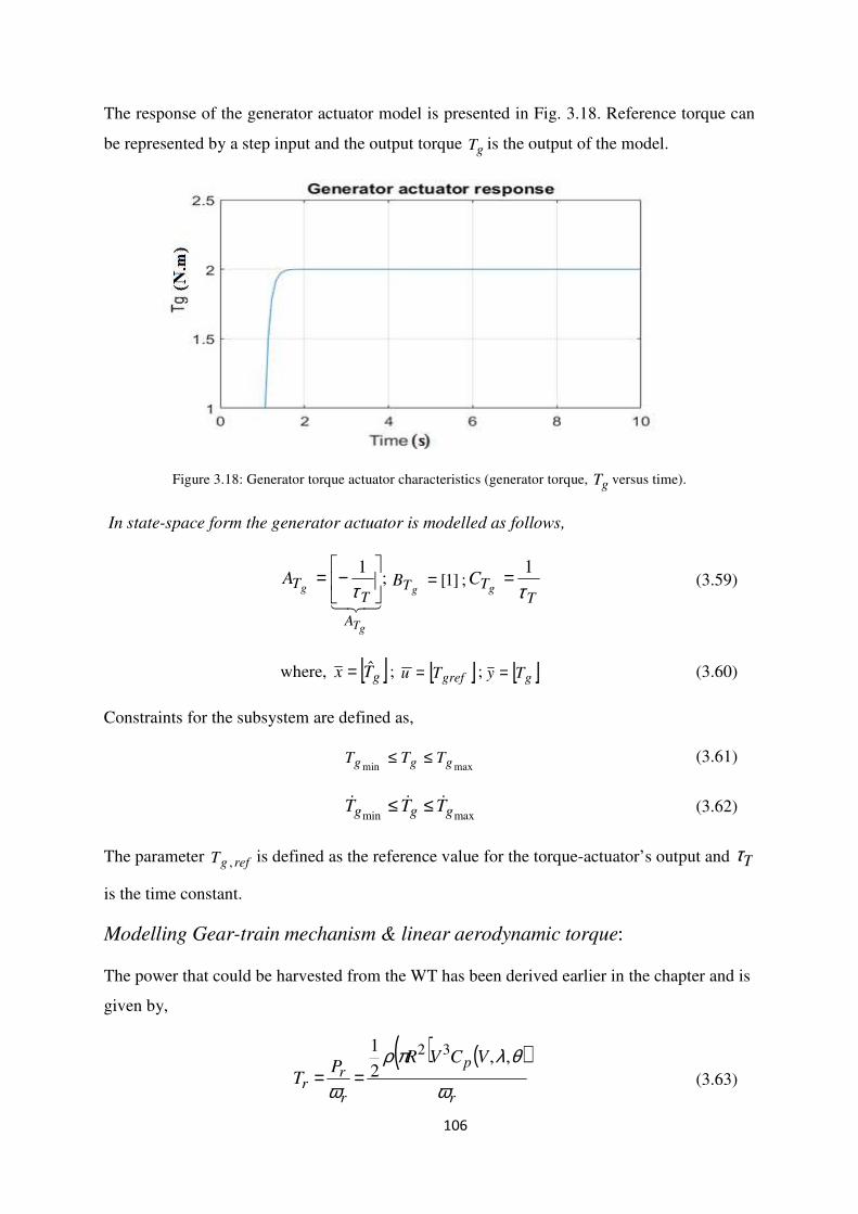
3.14 Modified pitch controller characteristics. 100 3.15 Hydraulic actuator motor model. 104 3.16 Pitch actuator response to the reference pitch angle with time. 104 3.17 Generator torque actuator Simulink block diagram. 105 3.18 Generator torque actuator response. 106 3.19 Wind turbine gearbox and the generator. 109 3.20 Simulink block diagram for the turbine shaft and the generator
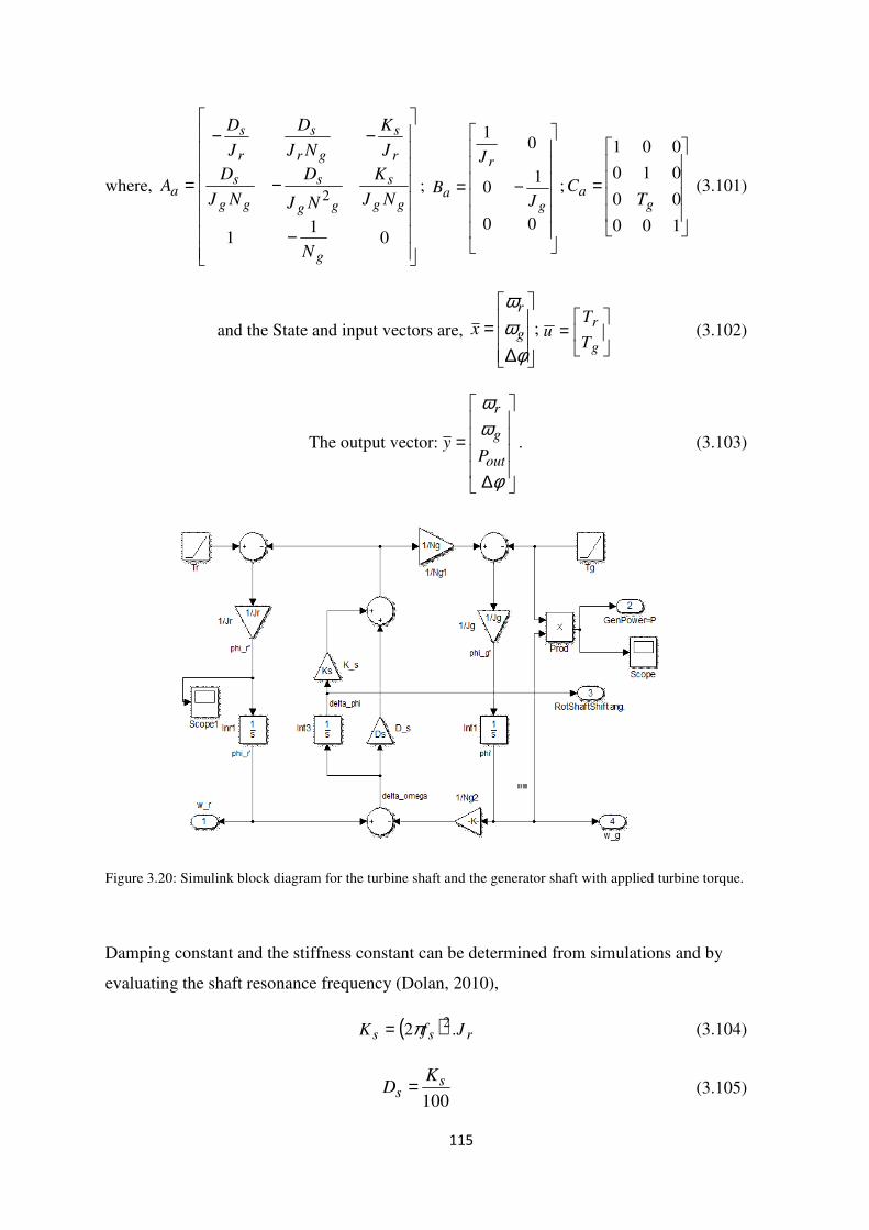
shaft with applied turbine torque. 115
3.21 Simulink block diagram: the total state-space system of the WT. 121 3.22 Simulation results of rω and gω versus time(s) for the total state-
space system.
122
3.23 Generated power versus time(s) characteristics of the total state- space system.
123
3.24 Characteristics of φ∆ versus time(s). 123 3.25 PID/State-feedback controller implementation results. 125
Page 10
10
3.26 PID/State-feedback controller for the turbine speed and generator speed control.
126
3.27 Schematic Diagram of a DFIG. 127 3.28 Simulink Block Diagram for DFIG. 134 3.29 Torque versus time(s) characteristics. 134 3.30 Generator torque characteristics versus Slip. 135 4.1 Wind turbine power versus wind speed and the illustration of
wind regions 147
4.2 Implementation of the MPC controller using Simulink toolbox. 150
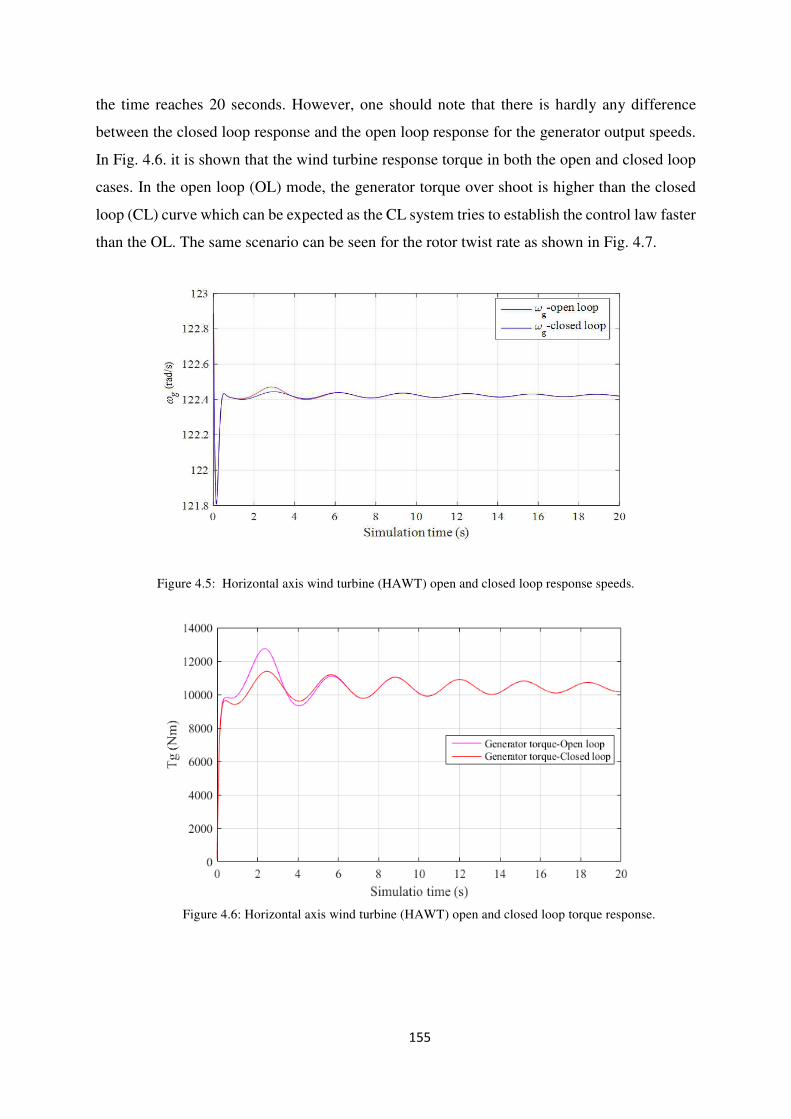
4.3 Input Signal to the Plant. 150 4.4 WT plant output characteristics with the MPC controller 151 4.5 Horizontal axis WT open and closed loop (CL) speeds. 155 4.6 Horizontal axis WT open loop (OL) and CL response (Torque). 155 4.7 Horizontal axis WT open loop & CL rotor twist rate. 156 4.8 Closed loop power output. 156 4.9 Pitch angle variation (open and closed loop demanded blade
angle. 157
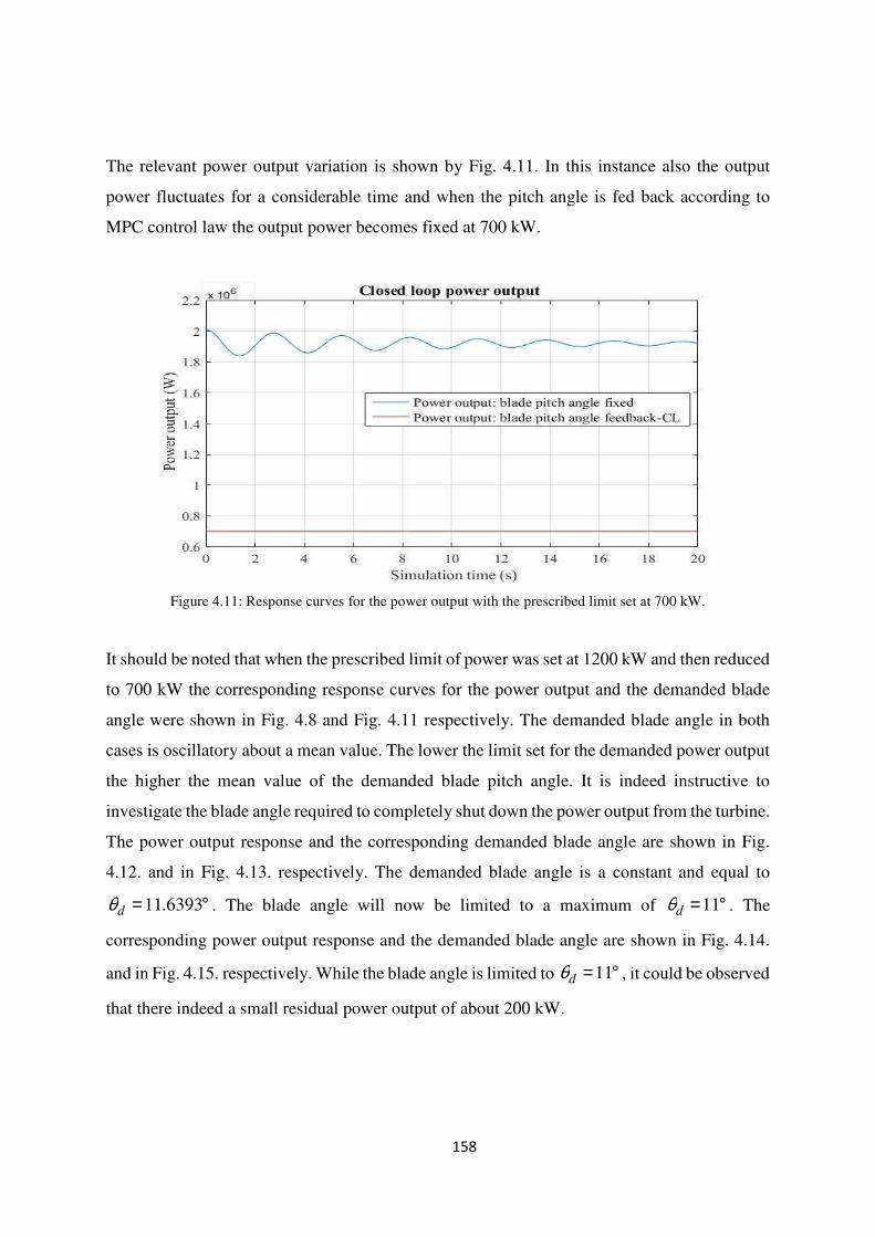
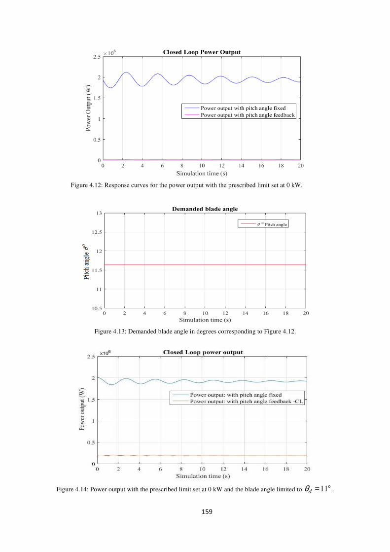
4.10 Demanded blade angle corresponding to Fig. 4.11. 157 4.11 Response curve for the power output (for 700kW) 158 4.12 Response curve for the power output with the prescribed limit of
0 kW. 159
4.13 Demanded blade angle in degrees corresponding to Fig. 4.12. 159 4.14 Power output with the prescribed limit set at 0 kW and blade
angle limit 159
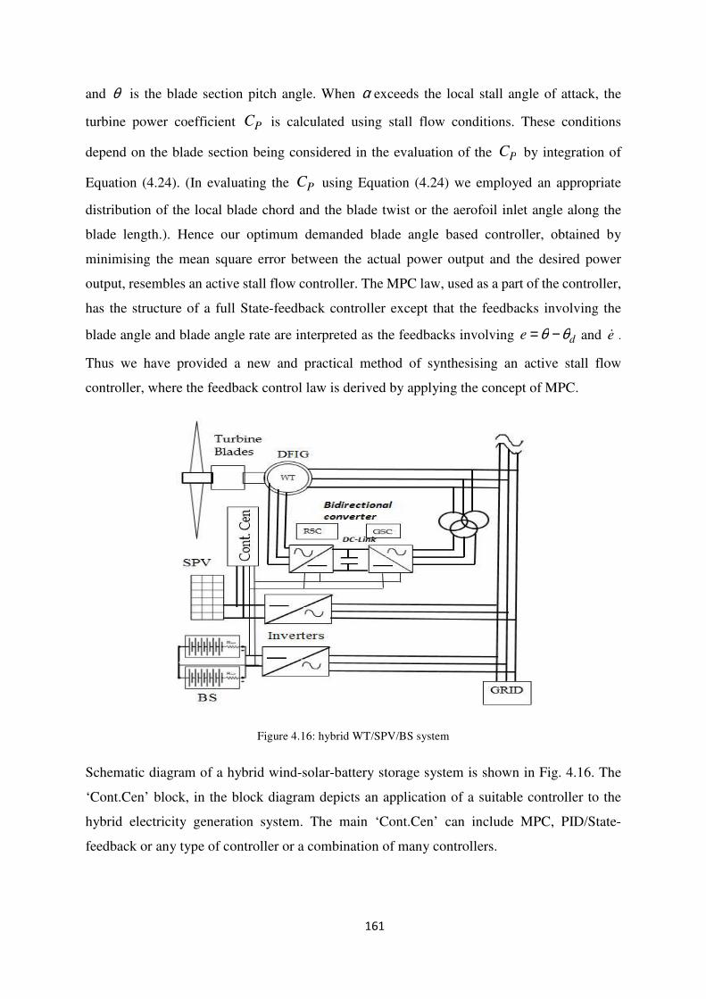
4.15 Demanded blade angle in degrees corresponding to Fig. 4.14. 160 4.16 Hybrid WT/SPV/BS system 161 5.1 Grid-Side converter arrangement. 164 5.2 Grid-Side converter and Rotor-Side converter connection with the
DFIG. 165
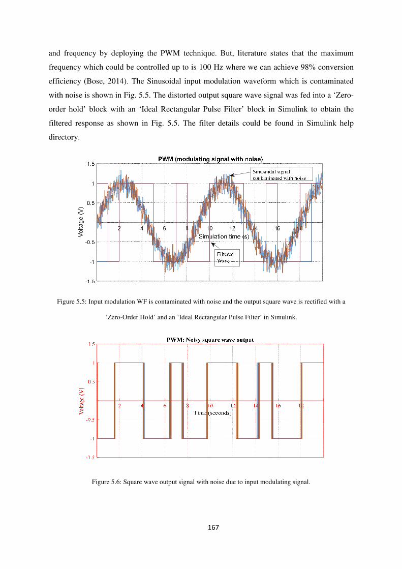
5.3 The principle of PWM (Input/Output waves). 165 5.4 The Simulink block diagram for PWM wave forms 166 5.5 Input modulation WF is contaminated with noise and the output
square wave is rectified 167
5.6 Square wave output signal with noise due to input modulating signal.
167
5.7 Simulink block diagram for the filtered square wave output by Ideal Rectangular Pulse Filter
168
5.8 Square wave output signal is filtered by Ideal Rectangular Pulse Filter and a Zero-Order Hold blocks
168
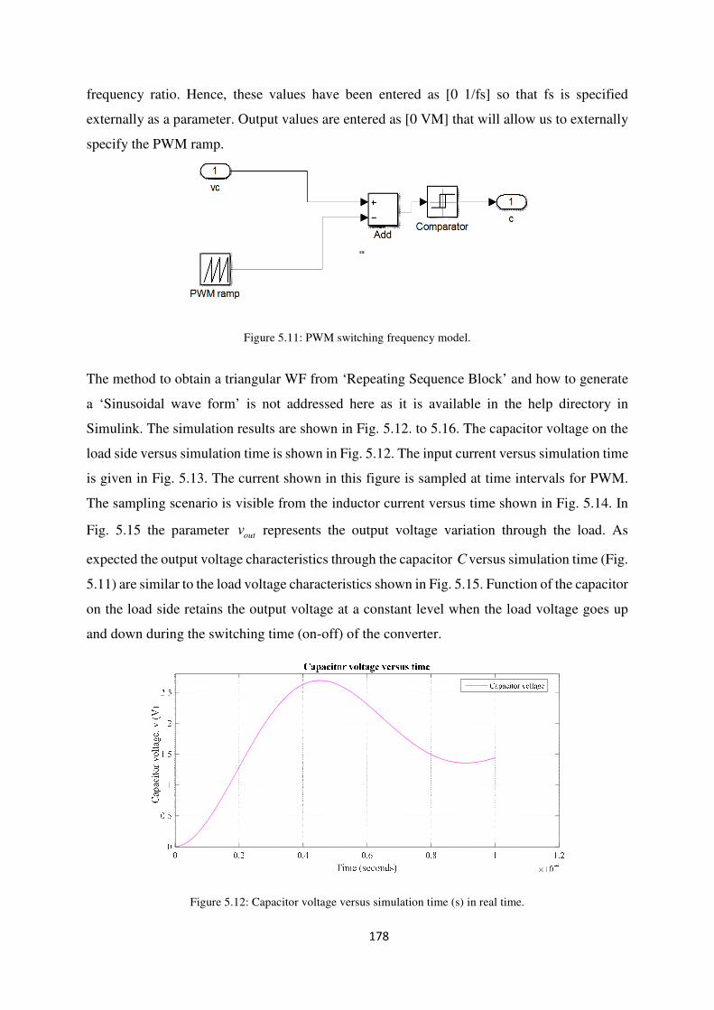
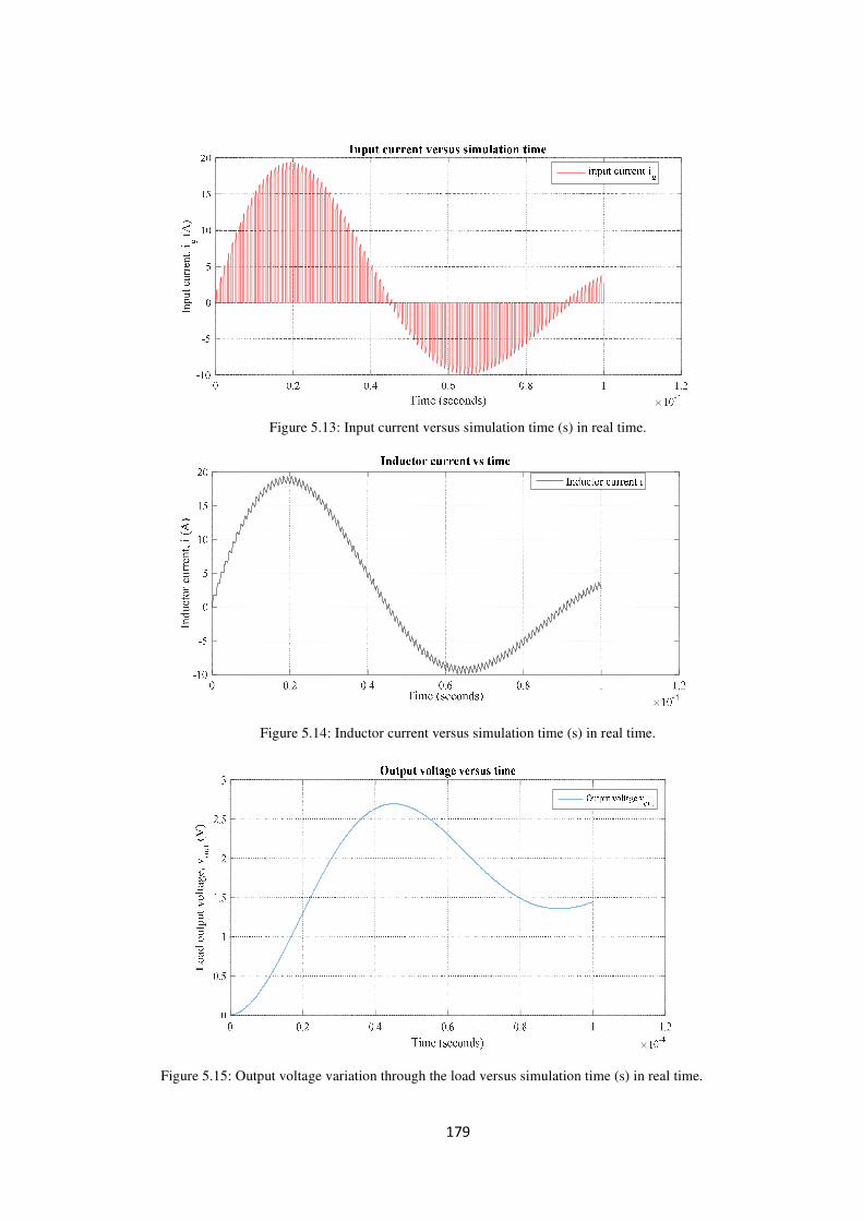
5.9 Simulink block diagram for the synchronous buck converter. 175 5.10 Synchronous buck converter circuit diagram. 176 5.11 Simulink PWM switching frequency model. 178 5.12 Capacitor voltage versus simulation time (s) in real time 178 5.13 Input current versus simulation time (s) in real time. 179 5.14 Inductor current versus simulation time (s) in real time. 179 5.15 Output voltage variation through the load versus simulation time
(s) in real time. 179
5.16.a Capacitor integrator and inductor integrator with initial conditions.
180
Page 11
11
5.16.b Capacitor integrator and inductor integrator with initial conditions (enlarged figure).
180
5.17 Averaged model of the of the Converter. 181 5.18 Buck converter open-loop control to output magnitude and Phase
response. 182
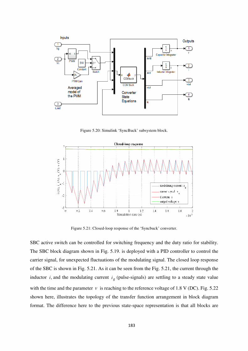
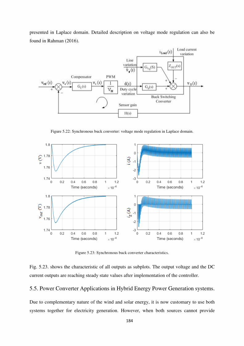
5.19 Buck converter closed-loop control with a PID controller. 182 5.20 Simulink ‘SyncBuck’ subsystem block. 183 5.21 Closed-loop response of the ‘Syncbuck’ converter. 183 5.22 Synchronous buck converter: voltage mode regulation 185 5.23 Synchronous buck converter characteristics 184 6.1 Physical structure of a PV cell. 188 6.2 Single diode equivalent electrical circuit for a PV cell. 189 6.3 The variation of Vpv versus Ipv at Constant Irradiance. 192 6.4
PVV versus PVI at constant ambient temperature. 192
6.5 PV module power curves at constant temperature. 193 6.6 Module voltage versus extracted power. 193 6.7 Maximum power point tracking (MPPT) points for varying
irradiances 195
B.1 Simulink block diagram for PV module. 228 C.1 Gaussian distribution. 231 C.2 Gaussian distribution-2. 232 C.3 Simulink Block diagram for Weibull wind distribution. 235 C.4 Weibull wind distribution. 235
List of Tables
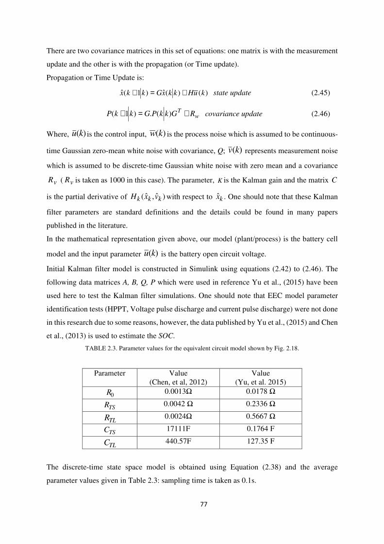
2.1 New constants in Equation (2.9) to Equation (2.13). 52 2.2 Panasonic 17500 Li-ion Battery Parameters. 57 2.3 Parameter values for the equivalent circuit model shown in Fig.
2.18. 77
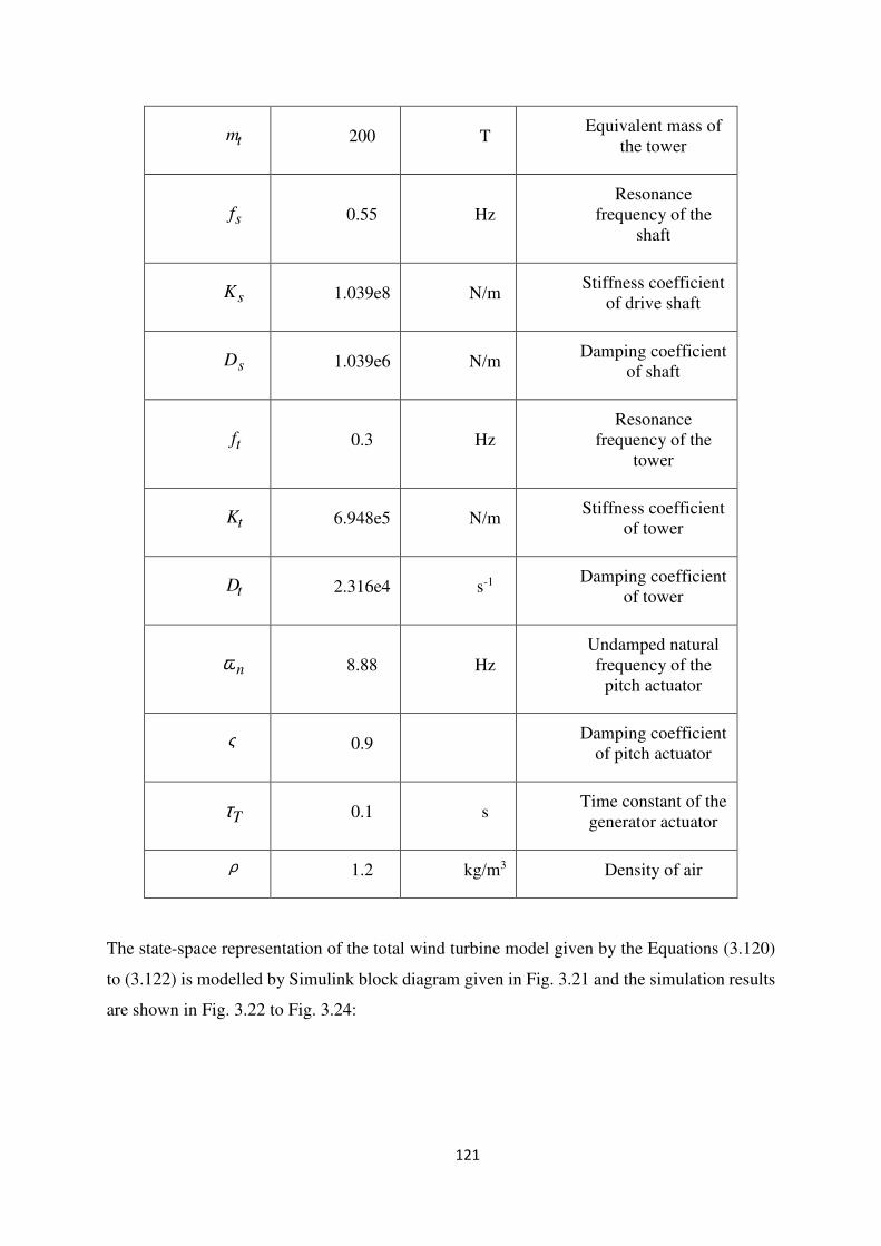
3.1 Wind turbine data. 120 4.1 Typical parameters and initial state values for simulation of a WT. 154
Acronyms
AC Alternating Current ANN Artificial Neural Network BEM Blade Element Momentum BP Battery Pack BS Battery Storage BW Bandwidth CB Capacitor Bank CC/CV Constant Current/Constant Voltage CCF Capacity Correction Factor CSP Concentrating Solar Power DC Direct Current DFIG Doubly Fed Induction Generator
Page 12
12
EKF Extended Kalman filter EU European Union EV Electric Vehicle FC Fuel Cell FLC Fuzzy logic control GA Genetic Algorithm GS Gain scheduling GSC Grid side converter HAWT Horizontal Axis Wind Turbine HE Hybrid Energy HES Hybrid Energy Systems HEV Hybrid Electric Vehicle HRES Hybrid Renewable Energy System ICT Information and Communication Technology INC Incremental conductance LIDAR Light detection and ranging Li-ion Lithium-Ion batteries LPV Linear parameter varying MPC Model Predictive Control MPP Maximum Power Point MPPT Maximum Power Point Tracking NMPC Nonlinear Model Predictive Control OC Open Circuit P&O Perturb and Observation PEV Plug in electric vehicle PHEV Plug in hybrid electric vehicle PI Proportional Integral (PI) PID Proportional Integral & Derivative PLL Phase Lock Loop PMSG Permanent Magnet Synchronous Generator PV/SPV Solar Photovoltaic PWM Pulse Width Modulation RC Resistor/Capacitor RO Renewable Obligation RSC Rotor side converter SBC Synchronous buck converter SCADA Supervisory control and data acquisition SEI Solid-Electrolyte Interphase SG Specific gravity (kg/m3). SOC State of Charge SOD State of Discharge SOFC Solid Oxide Fuel Cell SPV Solar Photovoltaic UAV Unmanned aerial vehicle UKF Unscented Kalman Filter VAWT Vertical Axis Wind Turbine VSC Voltage Source Converter WF Wave form WT/WTs Wind Turbine/Wind Turbines
Page 13
13
Symbols x State vector
1−kx Previous state
initSOC Initial state of charge
usableC Usable battery capacity (Ah or mAh)
cellT Electrolyte temperature in a battery cell in degree Celsius/or Kelvin
x Estimated state vector
ambT Ambient temperature in degree Celsius/ or in Kelvin
t discharge/charge time (s) k Time step t∆ Time step or sampling time (s)
bati Battery current (A); )(ti and i also denoted as battery current
pC Specific heat capacity (J/kgK)
pC In chapter-3 this coefficient is identified as the turbine power-coefficient.
CheC Empirical constant (numerical)
1CheC Empirical constant (numerical)
pN Length of the optimisation window (Prediction horizon)
cN Control horizon dictating the number of parameters used to capture the future control trajectory
ik Current time (sampling instant)
λ Conductive heat coefficient (W/m2K)
Φ Current density A/cm2 )(ku Input vector
)(ku∆ Input to the state-space model
)(kw White noise with zero mean and covariance wR q Number of output states
)|( ii kmkx + Is the predicted state variable at a time instant ( mki + ) and the
current plant information )( ikx at time instant ik .
)(kv Measurement Noise
S∆ Combined entropy change J/K
cS∆ Entropy change in cathode material (J/K)
aS∆ Entropy change in anode material (J/K)
mV Mean wind speed (m/s)
tv Turbulent wind speed (m/s)
rv Relative wind speed (m/s)
wP Wind power in the absence of a rotor disc (W)
rP Power absorbed from the wind to rotor (driveshaft)(W)
eP Electrical power of generator from mechanical power (W)
A State matrix
Page 14
14
B Input matrix C Output matrix D Feedthrough matrix F Faraday constant (1 Farad = 1coulomb/volt) G State matrix H Input matrix I Identity matrix I Current (A): this symbol is used to indicate the current from
Simulink step input block. k Battery constant K Kalman gain P Covariance matrix Q Covariance matrix
1Z Impedance of cell1 (ohms)
OCV Battery open circuit voltage (V)
batV Battery terminal voltage (V)
1cV Cell1 output voltage (V)
SRint Battery internal resistance (ohms)
CYCR Battery cyclic resistance (ohms)
TSR Short transient resistance due to polarization (ohms)
TLR Long transient resistance (ohms)
TSC Short transient capacitance of the RC network (F)
TLC Long transient capacitance of the second RC network (F)
1V Voltage across the capacitor TSC measured in volts (V)
2V Voltage across the capacitor TLC measured in volts (V)
E∆ Change in voltage due to active material in the electrode (V)
CheC∆ Change in Voltage due to battery electrolyte (V)
),,( SOCnTRself Self-discharge resistance (ohms)
)(SOCVOC Battery open circuit voltage as a function of SOC (V)
simOCV _ Battery open circuit voltage from simulation results (V)
ExpOCV _ Battery open circuit voltage from experimental results (V)
tx Displacement of nacelle (horizontal) (m)
m& Mass flow of air (kg/s)
gN Gear ratio
PC Aerodynamic power coefficient (numerical value)
TC Aerodynamic torque coefficient
rJ Moment of inertia of rotor (kg.m2)
gJ Moment of inertia of generator (kg.m2)
sK Driveshaft spring constant (Nm/rad)
sD Driveshaft damping constant (kgm2/rad/s)
Page 15
15
tM Mass of part of tower and nacelle (kg)
tK Tower spring constant (Nm/rad)
tD Tower damping constant (kgm2/rad/s)
tF Thrust force on tower (N)
rT Aerodynamic torque from the wind to rotor (drive-shaft) (N.m)
gT Mechanical torque from generator to driveshaft (N.m)
gN Gear ratio
N Number of cells n Cyclic number
Pm Mechanical power from driveshaft to generator (W) R Rotor blade radius (m) T Temperature in degree Celsius or in Kelvin v Wind speed (m/s) α Heat transfer coefficient for forced cooling or convective heat
exchange coefficient W/m2K β Pitch angle (˚)
β Empirical constant (numerical)
Ω Resistance (ohms)
ε Radiation coefficient (the emissivity coefficient) η Generator efficiency (expressed as a % numerical value) η Battery constant σ the Stefan- Boltzmann constant (W m−2 K−4: generally taken as
5.6703x10⁻⁸) ξ Empirical constant λ Empirical number θ Collective pitch of rotor blades () λ Tip speed ratio (TSR)
rω Angular speed (velocity) of rotor (rad/s)
gω Angular speed (velocity) of generator (rad/s)
nω Natural frequency (of pitch actuator) (rad/s)
rφ Angular displacement of rotor (radians or written as rad)
gφ Angular displacement of generator (rad)
∆φ Relative angular displacement or torsion of driveshaft (rad) ς Damping ratio
qrψ Rotor oriented q-axis flux (Wb)
dsψ Stator oriented flux (Wb and Flux density is measured in Wb/m2) (Stator oriented d-axis flux)
qsψ Stator oriented q axis flux (Wb)
drψ Rotor oriented d-axis flux ρ Mass density of air (kg/m3)
Page 16
16
Chapter 1
Introduction
1.1. Background
It is a well-known fact that fossil fuel resources are depleting very rapidly and renewable
energy has been considered as a promising substitute for ever increasing energy demand
(Amusat et al., 2016; Eltiganin and Masri, 2015). The conventional fossil fuel (oil, gas and
coal) power plants not only emit harmful gasses to the environment but also increase the carbon
dioxide level in the atmosphere leading to global warming (Shivarama and Kumar, 2015).
Invariably, scientists are exploring effective methods to harness energy from the abundant wind
and solar renewables as substitutes to replace fossil fuel driven power plants. The vision has
not been for a short term solution but, for a viable sustainability (EU PARLIAMENT
DIRECTIVE 2009/28/EC) in the long run to avoid fossil fuels completely before they run out.
However, intermittent nature of this renewable energy (the wind and solar) poses several
challenges to the engineers and scientists to establish uninterrupted, reliable and continuous
power supply. One such problem is the Grid integration of these renewable energy electricity
generation systems. Another critical problem is to design energy storage systems using these
renewable energy conversion systems to supply reliable uninterrupted power for consumer
usage. Amusat et al., (2016) state that energy storage integration is very critical if renewable
energy power generation plants are to be incorporated into such systems. Maheshn and Sandhu,
(2015) reported that there is always a mismatch between the generated energy and the load
demand due to weather and climate changes when using the wind and solar renewables as
energy conversion systems. This can either be resolved by using energy storage systems (e.g.
battery storage systems) or by mixing the two systems as the wind and solar renewables are
complementary in nature.
The other requirement for implementing these renewable energy systems is the application of
modern technology and control systems to improve the plant efficiency and reliability. The
manufacturing companies, researchers in this area are now concentrating on developing new
control systems and advanced switching devices to improve the efficiency and reliability of
these wind/solar power plants.
Page 17
17
1.2. Modelling and control of WT, SPV arrays and BS systems.
Nowadays, mathematical modelling has become a common tool for dynamic system analysis,
optimization, design and control. However, modelling and controlling of these renewable
energy conversion systems like wind turbines, solar photovoltaic (SPV) arrays and battery
storage (BS) systems poses challenges to the engineers as these systems have nonlinear
parameters when presenting equivalent mathematical models.
One such good example is when modelling BS systems, it is necessary to consider the non-
linear battery parameters related to electrolytes with the temperature effects. Battery
parameters such as internal resistance, battery output voltage, battery capacity, cycle number
and state of charge change with the battery electrolyte temperature (Bhide and Shim, 2009;
Erdinc et al., 2009). Martinez (2007) states that wind energy conversion systems are very
different in nature and, when modelling wind turbines, researchers’ main problem is a lack of
data and insufficient information on control-system structures due to the strong competition
between wind turbine manufacturers. In this scenario many researchers model large capacity
wind turbines in a relatively simple form, neglecting some of the essential parameters that could
influence the reliability and the stability of the analytical results. Another obstacle that the
researchers have to overcome is the different engineering specialisms related to subsystem
modelling such as gear changing mechanisms and the gearboxes, wind turbine blades, aerofoil
studies, blade element moment theory, doubly fed induction generators (DFIG), power
converters, grid integration etc. Modelling SPV systems involves the study of chemistry and
power electronics and power converters and their close-loop control strategies.
This thesis is aimed at contributing some engineering specialist knowledge in modelling and
simulation of large capacity wind turbines (WTs), SPV arrays and BS systems. It is also aimed
at presenting comparative simulation studies of the models with experimental data available in
the research archives. Another focus of this thesis is to model each system independently for
controller applications, harnessing maximum power while considering the stability. Without
presenting any critical reviews at this stage, it is correct to mention with the existing knowledge
BS systems play an important role in quality direct current (DC) power supply and in back up
energy storage facilities. The investigation into current developments and literature search into
battery cell modelling and BP development would further encompass the goal of accomplishing
expected substantial contribution to the research community. Also, with the general knowledge
gained by reading newspaper articles, industry websites and by reading new product
Page 18
18
information published by the manufacturers (e.g. battery cars) it can be stated that lithium-ion
(Li-ion) batteries are superior to other battery types. Li-ion battery cell modelling, equivalent
electric circuit model concept, simulation and their applications are the other contextual points
come under the purview of this research. Significant contributions in this area are expected
with new mathematical formulations related to battery packs. The nonlinear behaviour of the
battery cell chemistry and how to extend the developed models for similar applications will be
explored after critical literature review. Temperature effect on nonlinear battery parameters,
modelling and simulations with an equivalent electric circuit model are the other areas
considered for specific investigations in this research.
Other important area considered in this research project is the application of model predictive
control (MPC) which is an optimal control technique when many parameter constraints are
involved with controlling and optimizations. Wind turbine pitch angle control which is
famously known as pitching by WT manufacturers is considered for specialism in addition to
the BS systems. Eventually, the extensive study will be focussed in harnessing maximum
power at any desirable wind speed for WT designs and control techniques. Stall control of the
WT and the application of MPC control with the blade pitch angle is the other area that will be
explored for new findings and developments in this research. With the above pre-contextual
broad guidelines and boundaries specified at the inception, the following sections describe the
critical literature review related to BS systems, WT control, MPC control, PV arrays and Power
converters.
1.3. Literature Review and recent developments
1.3.1. BS Systems
Numerous battery types and battery cell models have been reported in the literature. Research
in new battery technologies has been increasing steadily as the demand for various applications
differs from each other. This section presents a literature review on battery cell models,
equivalent electrical circuit (EEC) models and BS systems.
Bao (2012) states that there are two types of battery models reported in literature and they are
the modified Shepherd type mathematical model and the circuit-oriented battery model.
Polarization effect and the use of Peukert’s equation has been emphasized in Bao’s approach
for building an effective mathematical model. The model described in this reference was for
Page 19
19
lead-acid batteries and has to be modified if the model is to be used as a generic battery model.
In addition, it is further reported that the extracted battery model using regression technique
had inconsistent results. Tremblay and Dessaint (2009) had presented a mathematical battery
cell model which is ideally similar to the model presented by Bao (2012). In both presentations
(where they used the modified Shepherd equation) they had assumed that battery cell
temperature does not change due to discharging/charging current and the battery internal
resistances have been assumed to be constant during charging/discharging. Tremblay and
Dessaint (2009) further identifies that the exponential part of the battery output voltage versus
battery capacity curve can be used to represent the lithium-ion battery discharge characteristics.
However, it is noted that the portion of the curve is a small percentage of the battery voltage
drop with respect to the battery capacity which can be insufficient for simulation studies. Gallo
et al., (2013) used the same modified Shepherd equation for their experimental analysis in Pb-
acid batteries. However, Gallo et al., (2013) used genetic algorithm (GA) Sequential Quadratic
Programming (SQP) to find out an optimal solution for battery parameters. The “Global
Optimisation Toolbox” in MATLAB was used to find the optimal solution. The battery model
presented by MathWorks Inc., (2013) was based on the model developed by Tremblay and
Dessaint (2009). In addition, there are some new features included recently in the MathWorks
Inc. model (e.g. battery cell temperature effect, ambient temperature, electrolyte type etc.).
Zoroofi (2008) described that battery models can be classified into five main areas: (i)
electrochemical (ii) equivalent electric-circuit (EEC) (iii) dynamic lumped parameters battery
model (iv) hydrodynamic, finite element type (v) Tabulated battery data used models. He
further states that among these model-types only the electrochemical and the EEC types are
widely used for analysis and simulation studies. Electrochemical models extensively use the
modified Peukert equation or modified Shepherd Model Equation.
Chen and Rincon-Mora (2006) stated that electrochemical models are mainly used by battery
manufacturing companies to optimize the battery design parameters related to battery open-
circuit voltage, current, microscopic concentration distribution of the electrolytes etc. They
specified that the electrochemical models are complex and computationally time consuming as
the models are formulated with coupled time-variant spatial partial differential equations. In
addition, Chen and Rincon-Mora (2006) described that, mathematical models do not offer
battery current and voltage variation characteristics which are important for circuit simulation
and optimization studies. They (Chen and Rincon-Mora, 2016) further highlighted that the EEC
Page 20
20
model has become a favorite candidate for modelling and simulation studies due to the intuitive
nature and versatility to represent the battery chemistry when all circuit elements are assembled
into one circuit. They are accurate enough to capture the non-linear behavior of the battery
chemistry using active and passive circuit elements like voltage sources, capacitors and
resistors. Finally, Chen and Rincon-Mora (2006) presented two RC networks in series with a
resistor and a voltage source to represent the EEC. Two RC networks represent the slow
transients and the fast transients of the electrolyte chemistry of the battery cell. Though, the
battery self-discharge and the battery life were modelled by a separate RC network, and with a
current source, Chen and Rincon-Mora (2006) neglected the slow transient effects and
forwarded a reduced order model at a later stage. Zoroofi (2008) presented an RC network with
a voltage source and a series resistor. However, Zoroofi’s (2008) model used two diodes
connected in reverse bias and forward bias method in the RC-loop for battery
charging/discharging.
He et al., (2011) emphasized that among the many types of battery models, that the Li-ion EEC
model had produced very accurate and repeatable dynamic simulation results. He et al., (2011)
used experimental data and the Genetic Algorithm to identify the battery model parameters.
Robust extended Kalman filter (REKF) has been used to testify the SOC values and for
sensitivity analysis of the initial SOC values. The improved dual polarization (DP) circuit
model which was presented by He et al., (2011) was a Thevenin’s model with an extra RC
network. Generally, a Thevenin’s model has a single RC network in series with a resistor and
a voltage source (He et al., 2011). The two capacitor RC model presented by He et al., (2011)
was the same mathematical model used by Valerie et al., (2001) at the NREL (NREL/CP-540-
28716, USA.) in 2001. Shamsi (2016) presented two RC networks with a series resistor and a
voltage source to represent the EEC model. For parameter identification, Shamsi (2016) used
a Panasonic NCR 18650B Li-ion battery cell, widely used by many researchers for their
experimental studies. Pulse Current Discharge test and continuous discharge tests have been
used by Shamsi to identify the battery cell parameters for the EEC model. Shamsi (2016)
further described how the two resistors in the RC-network model can contribute to the Faradaic
effect, including the charge transfer resistance. Two capacitors were used to model the surface
effects at the battery electrodes and the internal chemical kinetics or charge transfer kinetics
through the electrolyte of the cell.
Page 21
21
Shamsi (2016) and Thanangasundram et al., (2012) used similar types of EEC models and they
both used the hybrid pulse power characterization test (HPPC) which is sometimes identified
as the pulse current discharge test to identify the battery cell parameters. Shamsi’s (2016)
battery parameter test results are similar to the test results forwarded by Chen and Rincon-Mora
(2006). Erdinc et al., (2009) presented a two RC network battery EEC model which can model
the cyclic effect and the capacity fading. The empirical formula presented by Erdinc et al.,
(2009) for the cyclic resistance varies with the squire root of the cycle number. The cyclic
resistance in this model is connected in series with the battery internal resistor. In Erdinc et al.,
(2009) model, cyclic resistance variation with the temperature is also addressed by presenting
an empirical formula.
Gao et al., (2002) presented Thevenin’s EEC model for dynamic simulation studies of Li-ion
battery cell. The main difference in this EEC model is the inclusion of an additional voltage
source to represent the equilibrium potential due to temperature effect. In battery chemistry,
the equilibrium potential is defined as a fractional increase of the battery open circuit voltage
when charging or discharging process is completed. The amount of active material remained
at the electrode-surface can increase the open circuit voltage after some time due to temperature
effect or due to ongoing chemical reactions at the electrodes. Furthermore, Gao et al. had
presented the thermal energy balance equation applicable to the battery cell and the battery
open circuit voltage as a function of the battery current and the cell temperature. However, the
detailed analytical approach was not presented there for state of discharge (SOD) and battery
output voltage in terms of temperature and battery current which were reported as functions of
simulation time.
The experimental analysis has shown that the lithium-ion (Li-ion) batteries have extended
cycling ability (2000-5000 cycles) than other existing battery types (Wu, Y. 2015). They are
lighter than other batteries for a given capacity (battery capacity is a measure of charge stored
in a battery under certain conditions and is measured in ampere-hours (Ah)). Li-ion chemistry
delivers high open circuit voltage and low self-discharge rate. Opitza et al., (2017) in their
review article compared many commercially available battery types such as lead-acid (Pb-
acid), Ni-Cd, Ni-MH and Li-ion. Their review further states that Pb-acid batteries are relatively
less expensive among automobile battery systems but the manufacturers use toxic materials, as
well as Pb-acid batteries, exhibit lowest energy density (energy density in a battery cell is
expressed as mAh/g). The volumetric capacity of a battery is also another measure that can be
Page 22
22
used to compare how good the battery is. It is a measure of energy stored per unit volume. (for
battery cells volumetric capacity is measured in mAh/cm3). Opitza et al., (2017) reported that
Li-ion battery is a good candidate among battery types due to its highest energy density, safety,
longer cycle life with no memory effects. Jaguemont et al., (2016) described that though, Li-
ion batteries have become one of the best choices for electric vehicles and for many other
applications, their performance at very low temperatures has been very poor (e.g. below -200C).
Other major concern reported there was the performance loss and degradation due to cycling
and ageing.
Li and Mazzola (2013) presented a battery pack (BP) modelling approach considering only the
external measurements and the characteristics of a battery module (battery module is identified
as more than two cells connected either in series or in parallel. BP comprises battery modules
connected in series/parallel). Though, it is too early to analyse the literature regarding BP
modelling, the method reported by Li and Mazzola (2013) is discussed here, as their model is
a mixture of both BP and battery cell modelling. Their BP modelling technique is based on the
bandwidth experimentation for the BPs. The BP is modelled into two RC networks connected
in series with a series resistor and a voltage source similar to the battery cell model given by
Chen and Rincon-Mora (2006). The two RC networks BP model parameters were estimated
using sequential quadratic programming technique. Popular Panasonic CGR18650, 3.6V
(nominal voltage) standard capacity of 2450 mAh Li-ion battery cells were used by Li and
Mazzola (2016) also for the experimental analysis.
Makinejad et al., (2015) emphasised that battery internal resistance varies due to cycling,
ambient temperature, SOC and ageing. A series resistor connected with a single RC network
was presented as their EEC model. Mean square error minimization method was used to
investigate the battery cell parameters after initial calculations were performed in off line mode.
The experimental analysis shows that the battery internal resistance, open-circuit voltage
changes due to cycling and SOC. The results conform to the previous literature presented by
Erdinc et al., (2009) and Chen and Rincon-Mora (2006). Makinejad et al., (2015) concluded
that in large format of Li-ion batteries the battery internal cell temperature varies locally. The
temperature changes and the concentration gradients near the electrodes can change the battery
internal resistance and the cyclic resistance. The temperature gradients can be in the range of
0.2-0.90C within the electrolyte. Though they have presented experimental data for cycling
versus open circuit voltage, battery capacity etc. analytical presentations or empirical
Page 23
23
formulations were not given for further analysis. In contrast, Li and Mazzola (2016) concluded
that their BP model is an accurate model (with two RC networks) while ignoring cycling,
temperature, ageing and lithium plating effects on individual cells. Hence the battery pack
model presented by Li and Mazzola (2016) should be modified in order to use for repeatable
cycling, aging, variable temperature and variable current.
Smith (2006) reported that computational fluid dynamics (CFD)-type model validates the low
order battery models and estimation algorithms. He further states that CFD type model
validation is useful, as it is not physically possible to measure concentration/potential
distributions inside a battery and thus directly validate the estimates. Smith has not described
any EEC models though he had presented an exhaustive mathematical analysis on model
reduction techniques.
Xiong et al., (2011) presented a Li-ion battery model which is suitable for electric vehicles with
32V and battery capacity of 12Ah. They have combined a single RC network and a series
resistor with an open circuit voltage source which is modelled by Nernst equation. The Nernst
equation models the electrochemical characteristics and the polarization effects. According to
Xiong et al., (2011) the model parameter values identified have been considered as constants,
though they are functions of the temperature (measured in degree Kelvin) when actual Nernst
equation is applied to battery chemistry.
Literature review in this section briefly covers the areas in the application of thermal energy
balance equation, heat generation mechanism in the battery cell (application of Bernardhi
equation).
Makinejad et al., (2015) presented the heat generation mechanism in a battery cell in two
scenarios: irreversible Joule heating and the reversible heating. Irreversible Joule heating is the
summation of heat dissipated by each resistor. Mathematical relationships for the reversible
heating, application of thermal energy balance equation were presented in this article and the
thermal model was studied using MATLAB and COMSOL. Battery internal cell temperature
was observed by placing sensors. The generated heat in the battery cell is transferred by
conduction, convection and radiation. In their research article, it was assumed that the amount
of heat flow absorbed by conduction effect is taken as equivalent to the heat absorbed by
convection.
Page 24
24
Xiao and Choe (2013) presented the irreversible heat generation with two methods: one method
assumes the voltage difference between the open circuit voltage and terminal voltage includes
a sum of all voltage drops caused by electron and ion transport and chemical reactions; which
is simply expressed by the product of battery current multiplied by the difference between the
battery open circuit voltage and the battery output voltage. The battery open circuit voltage is
taken as a function of SOC. The mathematical formulation derived there is based on two terms
which are identified as heat dissipation by reaction kinetics and the ohmic heating. Both
reaction kinetics and the ohmic heating expressions were derived using electrochemical
formulations. In this research, they have taken that the reversible heat releases at discharging
is absorbed in when charging. Cho et al., (2014) used modified Butler-Volmer equation to
model the battery electrode current density in terms of electrode potential considering the
cathodic and anodic reactions separately. The current density changes with time especially
when the battery is discharging. This equation gives the detailed relationship of initial battery
cell current density, dynamic current density, the electrode potential and the equilibrium
potential at each electrode. Therefore, it is noted that the current density approach is an accurate
method of modelling when lithium plating and cycling is considered.
Viswanthan et al., (2010) reported that LiFePO4 based cells with either titanate or graphite
anodes can be used for thermal energy management of BP with cycling. The cycling process
according to battery chemistry, there is a cooling effect at the cathodes and while at discharge
there is a heat generation. Hence, for battery management systems, this pro-activity can limit
the charge-discharge currents to prevent the temperature effect increasing beyond
predetermined value. Sarre et al., (2004) reported the stability phenomena caused due to
passivation layer built at the electrode/electrolyte interface due to electrolyte reduction by
lithium. The other issue considered here was the growth caused by electron tunnelling through
the layer is irreversibly consuming lithium self- inhibiting due to thickness increase. This can
cause the battery to collapse due to extensive cycling.
The application of Nernst equation for low temperature phenomena with battery cell charging
and discharging is reported by Jaguemont et al., (2016). One dimensional energy balance
equation, applied to battery cell models, and the cycle aging dynamics are covered in the
review. Kroeze and Krein (2008) presented a three RC network EEC model that can be used in
different applications. The model presented was capable of predicting the characteristics of
battery current versus voltage and was ideally suitable for portable electronics and
Page 25
25
recommended not accurate for the transient response to short-duration loads (less than 1
second). Conductive and convective heat transfer models were given by Tan et al., (2011) with
the SIMULINK model. The experimental results had been obtained using with Panasonic
CGR17500 and Panasonic 4.2V, CGR18650 batteries. Model equations presented were based
on modified Tremblay and Dessaint (2009) model. Huria et al., (2012) described a multi-RC
network model which was identified as a complex model with computationally time
consuming. However, it was finally reduced to a single RC network, in series with a battery
internal resistance with a voltage source. Modified thermal energy balance equation had been
presented in the article, ignoring the Joule heating, reversible heating, conduction and
convective, radiation energy components. Finally, he had concluded that in a battery pack, cells
are generally combined into cell packs, whose thermal parameters are different from those of
single isolated cells.
Saiju et al., (2008) had presented an EEC battery model for Pb-acid batteries. Their model
comprised two RC networks, series resistor, a voltage source and a variable resistor connected
in parallel with the battery output voltage. The model is a combination of the EEC model
components with some SIMULINK blocks that represent the mathematical formulations of the
electrolyte behaviour. The specific gravity of the battery electrolyte was monitored during
charging/discharging process. During the charging and discharging the gas emitted by the
electrodes were taken into account to formulate mathematical relationships with the battery
current. However, battery open circuit voltage variation, battery output voltage variation versus
time characteristic curves did not show conclusive results with the manufacturer’s data. A
simple but comprehensive lead-acid battery model for hybrid system simulation was reported
by Ross (2011). Modified Shepherd equation, an empirical formula for battery open circuit
voltage versus electrolyte specific gravity (SG) variation characteristic curves were presented.
It was further noted that the experimental and simulation data presented by Ross was similar
to the battery manufacturer’s data.
During the recent past, many researchers have published various SOC estimation methods
suitable for many applications. Chang (2013) describes that accurate estimation of battery state
of charge (SOC) is a very complex and difficult process as there are many parametric
uncertainties due to limited availability of accurate models. The SOC is defined as the ratio of
current capacity to the nominal capacity. Mathematical methods of SOC estimation found in
Chang’s (2013) publication are: Open circuit voltage method, Terminal voltage method,
Page 26
26
Impedance method, Impedance Spectroscopy method, Modified Coulomb Counting method,
Neural network, Kalman Filter (KF), Coulomb counting, KF Combination method and the
Support Vector Machine method. Chang, further reported that Qmax Adaptation Algorithm
(which is a new computational algorithm) will substantially increase the SOC and the
remaining run time estimation accuracy. When compared both Coulomb counting method and
the modified Coulomb counting method, the only difference found there was the use of a
quadratic discharging current equation which is a function of charging/discharging time.
According to Chang (2013) the Support Vector Machine method (SVM) is an adaptive system
similar to KF, Fuzzy neural network method. The SVM method is suitable for highly non-
linear systems and is based on least-square estimation.
Pandey and Bansal (2012) presented two battery cell models (model one and model two)
involving thermal effects. In model one, the SOC variation with the battery internal cell
temperature, battery current, voltage gradient with cell temperature was reported. In model
two, modified mathematical formulations were presented and these were based on the
Arrhenius equation and Nernst equation.
An adaptive SOC estimation method based on unscented Kalman filter (UKF) algorithms for
lithium-ion batteries was published by He et al., (2013). The state-space parameter vectors A
and B had calculated off line by using the least-square method. Simulation results proved that
the application of UKF was more accurate than the extended Kalman filter (EKF). Han et al.,
(2009) presented an adaptive EKF based SOC estimation method for Pb-acid batteries.
Zhang et al., (2009) reported a combined experimental and Extended Kalman Filter (EKF)
recursive method to identify the battery parameters. Similar to the improved dual polarization
battery model presented by He et al., (2011), Zhang’s (2009) model comprised two RC-
networks. In addition, Zhang’s model had included the hysteresis effect and the equilibrium
potential. Zhang (2009) has assumed that the equilibrium potential is equal to battery open-
circuit voltage having given the battery to settle for one hour to observe final measurements
during experimentation. Zhang (2009) has not included the equilibrium potential variation due
to film, gas formation at the electrodes and the ambient temperature effects for more than one
hour.
When using KF for the SOC estimation or any other measurement estimation of nonlinear
parameters, the process covariance and measurement noise matrices are pre-determined
Page 27
27
(guessed values). If the guessed values are incorrect, then there will be large divergent
estimation errors. The other method of correcting large guessed-errors is to employ the
adaptive Kalman filter which uses the covariance matching method (e.g. Han et al., 2011). Lee
et al., (2007) presented a reduced order EKF method to estimate the SOC. They (Lee et al.)
suggested that by reducing the order of the EKF (reducing the number of RC networks to one)
could maximise the computational efficiency. Furthermore, it can reduce the calculation time
which is very useful for the SOC estimation in hybrid electric vehicle application. Pérez et al.,
(2015) reported an enhanced closed-loop SOC estimator for lithium-ion batteries based on
EKF. The speciality with this model is the inclusion of the hysteresis effect and the model had
been validated by using several current profiles. Nonlinear observer was used for the SOC
estimation by Xia et al., (2015). The function of the nonlinear observer is to verify the validity
of the proposed parameter identification method in the SOC estimation. Second order RC
network (two RC networks) had been used for the experimentation. The nonlinear least square
algorithm was used to evaluate the model parameters from collected data with the discharge
and rest processes.
BP model reported by Li and Mazzola (2013) was described briefly earlier in this review.
Ganesan et al., (2016) presented a reconfigurable BP model. Ganesan et al., (2016) not only
presented an electrochemical mathematical model but also presented an anode degradation and
capacity fading equations relating current density and the effective electrolyte conductivity
through the
formation of a solid-electrolyte interphase (SEI) layer. The definition of SEI layer can be
described when capacity fade occurs when cycle number exceeds thousands of cycles,
electrochemical processes are obstructed by the formation of a SEI in the negative electrode,
which compete with reversible lithium intercalation. The thermal model presented there was
based on the Bernardhi equation. Bruen and Marco (2016) presented a BP model in which cells
are connected in parallel. The state-space model which was representing a single cell was taken
as a building block to make the total state-space model according to the number of single cells.
Summary
Having analysed relevant literature, it can be concluded that the battery models with two RC
networks (e.g. He et al., 2011; Zhang et al., 2009) are popular among researchers as they can
offer sufficient accuracy with less computational burden. Among the battery types, it was noted
Page 28
28
that Li-ion batteries are promising candidates for further developments. Though, there are
several modelling methods available in literature, most models are application oriented but,
EEC models offered sufficient accuracy (within 1-2% error) and the flexibility to combine into
similar electric models for different analysis (Erdinc et al., 2009; Zhang et al., 2007 etc.)
It is further noted that the battery parameter variation due to ambient temperature and the Joule
heating effect has been neglected by many researchers in battery modelling. Among the battery
cell models in literature, only a few papers had addressed the temperature effect and the
application of Bernardhi thermal energy balance equation with the use of EEC model approach.
Application of the Bernardhi thermal energy balance equation for battery cell modelling will
also be focussed in this thesis.
BP modelling and design is the other emerging area where many researchers are still trying to
develop efficient, reliable energy storage systems. Having developed the battery cell model, an
extension of the circuit into a BP model will also be considered in this thesis. Battery models
presented by Saiju et al., (2008) and Ross (2013) will be revisited to analyse the validation as
the simulation results with Saiju et al., (2008) model was not in consonance with the
Manufacturer’s data for Pb-acid batteries. The SOC estimation has become an important battery
parameter for electric and hybrid electric vehicles as it is not possible to measure it directly.
State-space battery model presentation and the application of the EKF based SOC estimation
will also be examined and described in the thesis to add value to the research work.
1.3.2. Solar PV Arrays
Electricity generation using solar photovoltaic systems poses a unique challenge to improve
the efficiency while minimising the manufacturing cost. Research and development in this
area have been expanding as it is environmentally friendly and helping the planet to reduce the
greenhouse gases by reducing the carbon footprint. Thus, PV electrical power generation
systems have become more popular in sustainable energy research (Brever et al., 2015). A
Large number of research papers have already been published related to PV systems spanning
in the areas of solar power technology, economic aspects of solar power utilisation, dynamic
modelling of PV systems, maximum power point tracking (MPPT) systems, Grid integration
of PV systems, optimisation algorithms (Elmetennani et al., 2016). Research and development
are wide open to many in these areas as they are linked together to improve the applications of
renewable energy sources (Bhatnagar & Nema, 2013). However, within the boundaries of this
study, articles published in the areas of PV technology, dynamic modelling in solar systems
Page 29
29
related to MPPT and distributed grid integration with other renewables like wind, battery
storage systems have been considered.
The PV technology for grid connection and off-grid PV power plants has been reported by
Arsalan et al., (2016). In their publication, major emphasis was given to PV and concentrated
solar power (CSP) technologies. CSP technologies use mirrors and lenses to concentrate solar
power from a large catchment area and then it is projected in a form of a beam to convert the
solar energy to heat energy and electrical energy. Advantages of CSP technology versus PV
are also discussed by Arsalan et al., (2016). Recent advances in solar photovoltaic systems for
emerging trends and their advanced applications have been presented by Pandey et al., (2016).
Building integrated PV systems (Including outer brick walls), Concentrated PV plants, PV heat
energy generating plants, and PV desalinization plants are some of the applications reported
there.
Thin film solar cell manufacturing technology and how to minimise the manufacturing cost
was presented by Breeze (2008). The materials used for solar photovoltaic cell manufacture
and their efficiency have been reported in the articles published by Sankarganesh et al., (2012)
and in Tsang et al. (2013). Various internet sources could be found regarding microelectronic
manufacturing sector with the introduction of multi-junction PV cells and how these cells made
an impact to increase the efficiency of the solar array from 20% to 43.5% (Solar cell efficiency,
2013). However, Heriche at al., (2016) reported that, as at today, copper-indium-gallium-
diselenide (CIGS) cells offer maximum conversion efficiency of 25.9%. The chemistry behind
the achievement is different doping techniques of certain chemicals and absorbing layers.
MPPT systems using perturb and observation (P&O), hill climbing, evolutionary algorithms
were presented by Kamarzaman and Tan (2014). When environmental and shading conditions
change, application of conventional MPPT methods using P&O and genetic algorithms fail due
to rapid change of physical conditions and hence, neural network methods were proposed in
their research.
Sankarganesh and Thangavel (2012) implemented P&O MPPT system and Fuzzy control
mechanism to control the output power. Bhatnagar and Nema (2013) introduced a comparison
of computational algorithms in tracking maximum power while evaluating the parameters. The
parameters considered are the number of variables used in each algorithm, accuracy, the speed
of tracking the maximum power point (MPP), hardware implementation, cost, tracking
Page 30
30
efficiency. P&O algorithm, modified P&O algorithm, Incremental conductance (INC) method,
Fuzzy logic control (FLC) based, artificial neural network (ANN) methods, Gradient descent
methods were analysed in addition to a single diode equivalent electrical circuit used for
modelling a PV cell.
In addition, Bhatnagar and Nema (2013) described that though, P&O and INC methods are
widely used in the industry they have their advantages as well as disadvantages. The P&O
technique has the problem of oscillation around the MPP due to the trial and error
computational search method. Hence, a fair amount of absorbed power from the sunlight may
be wasted by trying to achieve the best for a shorter time of the day due to variable sunlight.
This problem can be reduced by using variable step size with the INC. The computational
algorithms described above are generally applied to non-linear VI − characteristic curves of
the solar panel. When the search is based on the voltage versus-time curve then it is defined as
the voltage based MPPT and when the algorithm is based on searching the MPP on the current
versus time curve then it is defined as the current based MPPT. In both methods, they use
DC/DC buck or boost converters to step down or step up the voltage. Other two methods used
to track the MPP are: curve fitting based MPPT and the numerical calculation methods.
It was noted that altogether they have reported more than thirty online and offline
computational algorithms used in practise for tracking the MPP with a PV array. Each method
has its advantages and disadvantages depending on the applications. Bhatnagar & Nema (2013)
finally concluded that the P&O and INC cannot calculate the MMP in one step as they are
iterative based algorithms and therefore, they are slow. FLC, ANN and particle swarm
optimization methods are good for when the inputs are not accurate and when the accurate
mathematical models are not available. They further concluded that the MPPT based on load
parameters method is better than the conventional methods.
Model-based rapid MPPT system for solar power extraction from a PV array was presented by
Tsang and Chan (2013) and by Meenakshi et al., (2006). Orthogonal least squares estimation
algorithm had been used with the experimental data to evaluate the parametric constants. MPPT
system using MATLAB as a programming tool was presented by Qin and Lu (2012). An
adaptive P&O algorithm was implemented for fast tracking by regulating the output voltage
after measuring the changes of output power. The single diode equivalent electrical circuit PV
cell model has been used in modelling the PV system. In order to improve the output efficiency
of PV system, a novel variable step size P&O method was emphasized by Qin and Lu to track
Page 31
31
the maximum power point of PV system. Grid connected PV system has been presented by
Chouder et al., (2013). The single diode PV cell model is extended into an array and the system
has been simulated using Lab-View. PV power generation system with a battery backup system
was presented by Ding et al., (2012). Their PV array was connected to a common DC bus by a
boost converter and the battery pack was then connected with a bi-directional DC/DC
converter. Finally, the converter power was connected to the AC grid by a common DC/AC
inverter. Hybrid Solar-WT system was presented by Meenakshi et al., (2006) to accommodate
the varying wind velocities and solar intensities. A neuro controller has been presented to
identify the MPP. A mathematical model for a single diode PV system has been presented by
Pandiarajan et al., (2011). SIMULINK has been used as a tool to analyse the system.
PV/FC/UC hybrid system was presented by Uzunoglu et al., (2009) with MPPT system for
solar energy harvesting. Two diodes equivalent electrical circuit model was reported by
Belhaouas et al., (2016) and Ishaque et al., (2011).
In literature for most applications and for modelling PV cell, current-voltage relationship
derived for single diode has been used. In other publications found in literature, same current-
voltage relationship derived for single diode has been used with minor modifications.
Approximate empirical formulations were presented for the generated power estimation by
Hocaoglu et al., (2009) and Mohammadi et al., (2012). PV arrays connected in series and
parallel were modelled by Tsai et al., (2008). It was further emphasized that two diodes EEC
model was not used in their research as there were some computing limitations to develop
expressions for the voltage-current curve parameters due to implicit and nonlinear nature of the
model.
Generally, the mathematical models for two diodes EECs are complex in nature and the
programmes frequently get into loops due to decoupled exponential functions. Hence, many
researchers have used the single diode equivalent electrical circuits for modelling PV systems
where the accuracy is sufficient to be compared with two diode model. Therefore, in this thesis,
a single diode model has been used to model PV systems.
Page 32
32
1.3.3. Wind Turbines Control
The production of clean electricity from renewable energy sources (the wind, solar, geothermal
etc.) has been promoted by many countries to tackle the current problem of green-house gases
and to reduce the dependence on fossil fuels. Wind energy is now gradually becoming one of
the most cost effective energy sources that can be converted into electricity. In the energy
transformation process, wind turbines (WTs) are initially used to harness mechanical energy
and then convert the mechanical energy, into electrical energy. Inherently, dynamics of the
WTs are nonlinear in nature and complex control procedures are needed for maximising energy
production while protecting the wind turbine (WT) components. In this section, a brief review
of advanced control methods on wind turbines is presented.
Aho et al., (2012) emphasized that WT control can be categorised into four main areas
according to wind regions (wind speeds). They are Region-1, Region-2, Region-3 and Region-
4. The Region-1 spans from start-up of the WT to the ‘cut-in’ wind speed where the generator
is turned on to produce electricity. Region-2 is defined as sub-region when the wind speed is
between cut-in speed and just below the speed where the wind speed is still insufficient to
produce maximum power. Region-3 is defined as the region where the wind speeds are high
enough to generate its rated power. At this region, the generator is controlled to regulate speed
and the power. The last region which is the Region-4, in which the turbine shuts down to
prevent damage. In the transition, the main aim is to capture the maximum available power
from the wind and it is harvested by controlling, blade pitch angle, turbine coefficient and the
tip speed ratio (TSR).
The blade pitch control is generally achieved by using proportional integral (PI) control. The
PI control system is designed to overcome the anti-wind up of saturation limits placed on the
pitch angle (Leith and Leithead, 1998). For optimum control of the blades, gain scheduling
(GS) is often used to adjust the PI gains with the pitch angle. Furthermore, GS will address the
nonlinear sensitivity of the turbine coefficient ( PC ) curve to blade pitch angle (Aho et al.,
2012). According to Leith and Leithead (2000), gain-scheduling design is described as divide-
and-conquer approach to nonlinear control systems to decompose into a number of linear sub-
tasks. Further, they have applied Lyapunov stability condition for velocity based linearization.
Cut-in speed and Cut-out speed are two commonly used technical terms in wind turbine
industry. The definition is as follows; ‘Cut-in’ speed: minimum wind speed necessary for the
Page 33
33
wind turbine to generate power (generally between 3-4 metres per second. ‘Cut-out’ speed:
maximum wind speed that the generator can operate safely. Beyond this speed, it is hazardous
to operate the generator.
Wake power, frequency regulation, active power control (APC) are the other areas addressed
by Aho et al., (2012). Hydraulic and DC motor actuators are used to control pitch angle and
the generator torque at reference levels. They further concluded that the researchers are still
investigating the strategies to balance aggressive power control demands against increased
actuator usage and structural loads.
Njiri and Soffker (2016) emphasized that WT control system hierarchy has three distinct levels;
namely, supervisory control, operational control, and subsystem control. They further reported
that the supervisory control manages the starting-up and shutting-down procedures while
operational control is concerned with the smooth functioning of the WT during its running.
The subsystem control deals with the pitching, yawing, actuation mechanisms and power
electronics. As pointed out by Njiri and Soffkor, (2016) though, 2H and ∞H controllers
extensively used for WT control, they are more suitable for robust tracking systems such as
disturbance rejection and noise suppression.
The review article presented by Wei et al., (2014) emphasized that GS can be applied to any
control system from process engineering to aerospace engineering. Some of the examples
reported there: gain-scheduled proportional-integral derivative (PID) control, 2, ∞ and
mixed 2/∞ gain-scheduling methods as well as fuzzy gain-scheduling techniques (Leigth et
al., 2001).
Multi-objective and model predictive approach controllers were implemented by Kusiak et al.,
(2010). The method deploys an intelligent WT control system based on data mining, model
predictive control, and evolutionary computation. To improve the quality of the controller, a
multi-objective model was presented. Multi-objective model is nothing other than adjusting
weights of objective control/operational parameters (in Kusiak et al., 2010) model five
objective weights) in response to the variable wind conditions. In their design, three control
factors, wind speed, turbulence intensity, and electricity demand had been considered in eight
computational scenarios. Genetic algorithm was used to calculate the optimal weighing
matrices of the LQG controller instead of using trial and error based Kalman filter gain and
state feedback gain estimation. The speciality with this application is the use of supervisory
Page 34
34
control and data acquisition (SCADA) to build the model whereas in the literature most
dynamic models are derived from first principles.
Application of GS technique for Linear parameter varying (LPV) systems was presented by
Bianchi et al., (2005). GS is particularly useful for WT control as the approach consists in
designing linear controllers for several operating points and then applying an interpolation
strategy to obtain the global control. Though, there were numerous applications for WT
controllers in nineteen-nineties, the method did not give systematic design procedures. Though,
the application of linear controllers by interpolating them to reach global control seems to be
favourable to handle all four wind regions, the method was not given extra publicity and
exposure by the manufacturers due to trade secrets. When applying the state-space method, a
similar method is followed, but the linearization is performed using Taylor series expansion
(see for example Larsen and Mogensen, 2006). The local controllers in the GS method use the
∞H optimal control tools due to multi-input multi-output nature of the parameters. Hence, the
predictive concept applied to model predictive controllers (MPC) can be considered as an
evolution from GS techniques. In GS, the Jacobian Matrix with the Euler equation are used for
linearization. In MPC Euler-Lagrange equations are used. In order to be able to perform control
in the whole spectrum of wind speeds, gain scheduling and MPC methods were applied by
Gosk (2010). In addition, the application of GS technique in frequency domain is a proven
method offering successful results when the pitch and torque actuators are subject to frequent
damping effects (Bianchi et al., 2005). GS can be applied to EKF to reduce the conceptual
burden in calculating the Kalman gain in every iteration (Horkheimer, 2012).
Leith and Leithead (2002) reported a novel nonlinear gain-scheduling control technique for
power regulation of a horizontal-axis grid-connected up-wind constant-speed pitch-regulated
wind turbine. An interesting point to note here is that the plant dynamics has been considered
adequately nonlinear and then transformed into linear systems while control objectives
remaining nonlinear. Multivariable control strategy for variable speed, variable pitch wind
turbine had been proposed by Boukhezzar et al., (2007). In this research, the nonlinear state
feedback torque control strategy is combined with a linear controller to control the blade pitch
angle. The proposed system has been identified as a better system than using a PID and LQG
controllers.
Page 35
35
Robust MPC controller for a wind turbine was reported by Mirzaei et al., (2012). The approach
was defined as a minimax robust MPC approach. When the wind speed is below the rated value
the WT is operating at MPPT mode and when the wind speed is above rated value then the WT
is controlled by regulating the output power. Blade element momentum theory is used to model
the power extracted from the WT blades and the EKF with Taylor series were used to estimate
the operating points.
Controlling the generator side plays an important role for stable power supply and maximum
power extraction from the WT at variable wind speeds. Most of the methods described so far
belong to the rotor side control or control systems related to the turbine blades. With the blade
side and the rotor side control (RSC) the power regulation, is achieved using State-feedback
torque control, blade pitch control, and with the generator speed control methodology. MPPT
with the wind speed, controlling the pitch, TSR, optimal torque extraction, output power
control are some of the control problems encountered in this section. Controlling these
parameters use the ‘priori’ knowledge of the optimum turbine coefficient. However, a perfect
estimate cannot be achieved using analytical or experimental methods. In majority of MPPT
algorithms, the pitch angle is kept constant and the PC is slowly determined by TSR.
Indirect strategy for the active and reactive power control for the rotor side of the WT using a
sliding mode controller was implemented by Cherfia et al., (2013). The dq-axis reference frame
was used to model the DFIG. Control of the rotor side converter, which is used to regulate the
active and reactive power exchange between the generator and the grid, is applied by indirect
decoupled control without falling into a power loop. In contrast, modified direct power control
(DPC) method to control active and reactive power was used by Jeong et al., (2008) without
using any d-q axis transformation. Jeong, et al., (2008) used the voltage vectors from a look-
up table to calculate the active and reactive power. Chen and Chen, P-H. (2014) used
bidirectional AC/DC converter which could work in rectifier mode and inverter mode to control
the active and reactive power of the DFIG.
Though, the performance improvement can be achieved by using fixed gain control methods,
some of the control techniques utilized to improve the maximum power lead to other analytical
and estimation problems. Some of them are: to calculate the TSR, wind speed is taken as an
input, however, it is difficult to accurately calculate the wind speed from direct measurements.
The P&O method does not need prior knowledge of the maximum power coefficient as it uses
Page 36
36
the hill climbing method to locate the optimum point from the turbine characteristic curves. It
was noted that P&O algorithm will also fail when there is a rapid variation of the wind speed.
In contrast, sliding mode control and extremum seeking control techniques take considerably
high computer iteration time to converge. Though, the system offered good reference tracking,
chatter in the gearbox was inevitable. To overcome these problems to achieve the optimal
control of torque and flux tracking, nonlinear sliding mode controller has been proposed at the
expense of zero error tracking (Njiri et al., 2016). They further state that it is not possible to
achieve both the efficiency and the reliability together for large WTs, as the two are conflicting
in nature. The fatigue and stresses of large WTs are due to excessive up or down movement to
adjust the reference of the pitch angle or demanded torque.
Schlipf et al., (2014) presented a comparison details of a linear and a commercial nonlinear
MPC to a baseline controller. They further reported that the nonlinear model predictive
controller achieved better results than the linear controller. Light detection and ranging
(LIDAR) remote sensing technique was used to obtain accurate wind field data as input
parameters ahead of time. Actually, LIDAR technology has been in existence since 1970s, but
due to extensive cost of the equipment, the technology extension was hampered. This sensor
measures the upwind speed before it interacts with the turbine, and hence turbine has sufficient
time to self-control with the necessary actuators to face the incoming wind. LIDAR was used
in advance to set the pitch angle and the generator torque. In contrast, Pao and Johnson (2009)
emphasized that new LIDAR systems based on solid-state sources and off-the-shelf
telecommunications equipment allow for inexpensive deployment, modularity, and improved
reliability. Furthermore, they described that turbines are built for variable pitch angles at
different radial positions along the blades relative to the standard blade twist angle.
Wind turbine model predictive speed controller based on identified piecewise affine discrete-
time state space model was reported by Hure (2016). The main advantage over the other
controllers has been emphasized as the predictive property and explicit integration of the
constraints in the control problem. The performance had been compared with a baseline line
controller through simulations for both below and above the nominal. Morari and Lee (1999)
presented an MPC review article on: past, present and future. The main intention of the article
was to present an overview of the origins of MPC and its glorious developments up to the year
1999.
Page 37
37
The DFIG with slip-rings, whose stator windings are directly connected to the grid and its rotor
winding are also connected to the grid through a bidirectional frequency converter using a
back-to-back pulse width modulation technique is modelled by Martinez (2007). Okoro (2003)
presented a complete dynamic model for induction machine which could be applicable for the
WT modelling with the d-q axis transformation theory and Park transformation matrix. Though
the model presented was for a motor, the same methodology could be used by changing the
slip for negative values to apply for DFIG modelling. Ekanayake et al., (2003) presented state-
space modelling of variable -speed wind turbine. Their systematic approach in state space
modelling included ‘current model’, ‘fluxes model’ and ‘rotor internal voltages and stator
currents model’. In each method, the state vector is defined as the dq-axis current states, fluxes
or fluxes with voltages. Ekanayake et al., (2009) used PI controllers to control the variable
voltage/current changes and Okoro (2003) presented an algorithm to control the flux saturation
effect.
Novak and Chalupa (2013) published a multiple MPC controller for WT control. The applied
method was especially favourable since it was applicable for some of the states which were not
measurable. The EKF was used to estimate the effective wind speed. The estimated states and
active model parameters were then used within predictive control strategy for computation of
control signals. A nonlinear model predictive control system was developed by Slegers et al.
(2006), to control unmanned air vehicles (UAV). The system designed had six degrees of
freedom. Unlike in the previous controllers in this system, the number of Taylor series
expansion terms was used to indirectly penalize the control action.
Summary
Concluding the critical review in this section, it was noted that though, the development of GS
started in 20 years ago, it did not spread into every possible system in engineering. Some of
them might have confined into WT control and self-guided or autopilot control systems. On
the other hand, manufacturing companies did not want to expose the detailed methodologies
due to trade secrets or competition (e.g. guided missiles; Wu et al., 2002). Based on the number
of research articles published recently, in the Journal of power sources, IEEE, and other reputed
control journals, the GS method seems to be gradually picking up with some practical
applications. However, not as fast as MPC control systems which at the moment are becoming
very popular among the emerging researchers. An another reason that can be pointed out is the
similarity of the linearization procedures at an equilibrium point and the MPC designs are
Page 38
38
modelled by using favourite state-space methods (of course, this statement doesn’t imply that
MPC systems are confined only to state-space models, but, MPC controllers are well applicable
to plants in frequency domain as well). With the state-space systems, there is a flexibility to
expand the systems into many different state-space models to build a total linearized model if
the subsystem dynamics are well modelled. In addition, the MPC Toolbox in Simulink allows
one to program and manipulate MPC controllers as MATLAB objects (though, MATLAB is
an another tool) through a variety of methods and functions for simulation, analysis, and tuning.
The linear MPC controllers can be embedded arbitrarily in complex MATLAB programs, with
maximum versatility (Bemporad, 2006). Rotondo (2016) reported the current advances in gain-
scheduling and fault tolerant control techniques. Rotondo (2016) was mainly focussed in the
area of gain-scheduling, and analysis of the connections between the linear parameter varying
(LPV) and Takagi-Sugeno (TS) paradigms.
Considering the literature boundaries and the time limit for this research, though, GS is also a
promising area, the application of MPC in WT control is mainly focussed in this research.
1.3.4. Hybrid Renewable Energy Systems
Literature review presented so far considered BS systems (or battery cell models), PV arrays
and WT control separately. All of these systems together can play an important role in
electricity generation as they are complementary in nature. Therefore, it is pertinent to describe
such combined renewable energy systems which are normally identified as hybrid renewable
energy systems (HRES). For hybrid system applications it is important to understand dynamic
modelling and simulation characteristics of WT, PV and BS systems independently. A brief
review on HRES is given in this section as most of the systems found in literature, elaborated
on WT/PV/BS systems.
In future, the demand for stand-alone micro-grids using PV arrays combined with wind turbine
generators/Fuel cells and BS systems will increase as they are sustainable and environmentally
friendly (Wang et al., 2008). Intermittent nature of these renewables can be addressed with
innovative control systems and switch power from wind energy to solar or solar to wind energy
or by utilising BS systems. The micro-hybrid system designed by Wang et al. could provide
adequate power for five households. They further emphasized that the output power was kept
constant when the wind speed is higher than the rated wind velocity even though the wind
turbine has the potential to produce more power. The pitch angle was controlled to protect the
electrical system and to prevent over speeding of the rotor. When the wind speed was higher
Page 39
39
than the ‘cut-out’ speed (25 m/s), the WT was shut down for operation due to safety reasons.
Though, the wind energy and solar power are essentially discontinuous, harnessing and supply
energy from them and marine current has become one of the most exciting emerging forms of
renewable energy. Unlike many other forms of renewable energy, marine currents produce a
consistent source of kinetic energy caused by regular tidal cycles influenced by the phases of
the moon. However, energy harvest from tidal cycles is also not without problems as there are
challenges due to the random power output variation. This can be alleviated through
conditional outputs and phasing between different locations. The scarcity of proper
geographical locations for tidal power generation (Commin et al., 2017) is another challenge
that the designers have to overcome.
Grid integration and electricity supply from renewable energy sources have been facing a
number of challenges. Especially, WT integration to the grid is a major challenge for power
companies: in particular, to ensure the power balance, security of safe maintenance, computer-
based remote control, automation systems development, smart metering, reactive power
control, frequency control, voltage variation, harmonics and PLL control (Martinez and
Aurelio, 2010). The unified state-space model (assembled for WT, BS, PV array and induction
generator) presented by Martinez and Aurelio, can work both under transient and steady-state
conditions. The model reported is presented with a complete schematic diagram of each
subsystem of WT, PV arrays, BS system, inverters, and the Generator unit.
The application of proportional integral (PI) and proportional integral and derivative (PID)
controllers has been reported in many research articles in hybrid renewable energy systems.
Application of PI controller programmed with P&O optimisation algorithm was published by
Kabalci (2013). In Kabalci’s research, the MPPT algorithm was used in the control step of the
converter which was developed using P&O algorithm with an extended PI controller. In most
of these hybrid systems, solar and the wind energy systems were widely used and they were
modelled separately and assembled together to build a distributed generation system.
Dali (2010) presented a technical description of hybrid system devices and of the inverter
energy management system. Dali’s experimental set up included a grid connected hybrid
system, the wind and photovoltaic (PV) physical emulators, battery energy storage, load and a
controlled interconnection to the Low Voltage (LV) grid. Wind turbine emulator with a
permanent magnet synchronous generator (PMSG) has been used for experimental work. The
PMSGs do not have the problem of cogging torque and robustness. DFIGs are generally used
Page 40
40
for higher capacities of power generation in the Mega-Watt range. Unlike in Kabalci’s (2013)
research article, Dali’s research paper had not included simulation results to compare with the
experimental results.
Jitendra et al., (2012) proposed a hybrid Wind/PV system to provide electricity supply for a
few household connections. The model designed by them was able to control the voltage,
frequency fluctuations, and their power usage. Ciobotaru et al., (2006) presented a PV inverter
control system and a single-phase PLL structure including grid voltage monitoring using
dSPACE. Fuzzy controlled power management strategies for a grid connected hybrid energy
system was presented by Kumar et al., (2014). The hybrid energy system presented included a
PV array and a Solid Oxide fuel cell (SOFC). Simplified single diode solar cell model and the
SOFC was modelled using Nernst's equation. Kumar et al, further emphasized that though there
are many MPPT techniques available in the literature such as incremental conductance (INC),
constant voltage (CV), and P&O, the P&O method has been widely used by many researchers
because of its simple feedback structure and fewer measured parameters.
Fuzzy based P&O algorithm was used by Sankaganesh et al., (2012) for MPPT of the PV
system. Standalone WT/PV hybrid system was presented by using HOMER software by
Badawe et al., (2012). Fuzzy-PID controller to control a WT/PV hybrid power system was
presented by Zhang et al., (2007). In this method, continuous power supply to the systems was
achieved by using the fuzzy intelligence controller which monitors the SOC of the BS system.
Cost optimization, analysis, energy management and reliability studies for hybrid energy
systems were reported in (Kaviani et al., 2009; Ahmed et al., 2011; Nandi and Ghosh, 2009).
Research forte in most areas has been the application of fuzzy controllers and neural networks
for system identifications. Fuzzy-PID controllers are also used to optimize the output power
and to reduce the cost of the hybrid systems as stand-alone units. Though some researchers
proposed the neural network models, sliding mode control and Lyapunov Functions with the
Kalman Filters. They are suitable to apply for specific situations where the measurements are
observable and for uncontrollable systems. For hybrid energy systems, they are still at the
experimental stage and yet to be assessed with the economic viability. The PI and PID control
systems are still very popular with WT control and DFIG control systems as they are cheaper
to implement.
Page 41
41
Summary
Application of MPC for hybrid energy systems can be found in many occasions emphasizing
as a promising area for research and development during the recent past (Bemporad, 2006).
Initially, the MPC systems have been widely adopted in the field of process control, and their
application and that has now been extended to unmanned air vehicles (UAV), aerospace
applications and hybrid energy systems (Khan et al., 2011; Slegers et al., 2006). The MPC also
offers the versatility to combine, EKF or Fuzzy controllers to arrive optimal solution to
numerical optimisation while manipulating future actions within the hard constraints.
Hence, in this research, more focus will be given to MPC design and application to WTs, DFIG
modelling and electricity generation with constraints.
1.3.5. Power Converters
Power converters are generally used for DC-DC conversion or DC-AC conversion. Nowadays,
high frequency switches working with the pulse width modulation (PWM) technique have
become very popular and extensively used in power electronics. There are three main basic
types of power converter used in electronic industry. They are Buck-converters, Boost
converters and Buck-Boost converters. These converters, are also categorised as switched
mode DC-DC power converters. In addition to the power converters, inverters also play an
important role in WT power generation systems which are connected to the grid. Inverters
convert DC power into AC supply. PWM technique is mainly used by the inverters. Dynamic
behaviour of the Buck, Boost, Buck-Boost converter is highly nonlinear due to the function of
the switch incorporated with.
Delimustafic et al., (2011) used a Buck-converter, AC-DC converter and a DC-AC converter
for their HRES design. In addition to the above three basic categories of the converter, a Cuk-
converter is sometimes used in WT industry for power conversion. Good description of AC-
AC and Dual converters can also be found in Bose (2014). Large scale wind turbines (over 1-
1.5 megawatt scale (MW)) are generally, coupled with doubly-fed induction generators (DFIG)
for electricity generation. In these generators, rotor winding is connected to the grid with the
back-to-back PWM voltage source converters (VSC) (Hess et al., 2000). Back-to-back
converter which is a bidirectional power converter, consists of a controlled rectifier and a
Page 42
42
controlled inverter. Schematic diagram for a stator-flux-oriented stator-side converter control
is given by Hess et al., (2000).
Matrix converter which is another type of converter used in WT industry, has a unique topology
of AC to AC converter does not require any intermediate DC conversion (Islam et al., 2013) to
connect to the Grid. Islam et al, compared the Z-source converter and the Matrix converter with
the Back-to-back converter. Islam et al., (2013) further reported that Cyclone converters are
generally used by offshore wind farms. Matrix, Two-level and Multilevel converter topologies
were presented with comparative control strategy and performance analysis by Melício et al.,
(2010) for wind energy conversion systems.
In addition to the back-to-back PWM-VSC, an innovative cost effective power converter was
proposed by Hess et al., (2000) which differs from other converters as it has only one bridge,
composed of active devices. It has half switching devices and the hardware components than a
conventional converter. Kumar et al., (2013) proposed a converter which is proficient for
energy diversification from renewable and storage energy sources individually or
simultaneously. It has the capability to operate either in a buck, boost, or buck-boost mode and
directionally. Kalanta et al., (2010) proposed a six-pulse inverter topology for their stand-alone
hybrid power generation system. The six-pulse-full -controlled rectifier is used to convert the
AC output of self-excited induction generator into DC voltage. Ciobotaru et al., (2006)
proposed an inverter model and it was tested using dSPACE control board.
The preferred use of buck-boost converter than Cuk-converter has been proposed by
Sankarganesh and Thangavel (2012). Limitations of Cuk-converter and how to improve it to
accommodate high voltage conversion ratio is explained there and hence a hybrid boost mode
Cuk-converter is proposed. Use of power converters in standalone hybrid energy systems has
been well defined and hence, the power converter proposed by Sankarganesh and Thangavel
(2012) and according to the reference of Babaei et al., (2014) is analysed in this thesis.
1.4. Motivation
The motivation for this study stemmed from (i) the passion for control systems, (ii) expected
benefits of renewable energy and (iii) real-life renewable energy plants.
One of the main problems of this planet is the burning coal, oil and gas which increases the
prevailing CO2 concentration at an alarming rate. On the other hand, the monopoly of the oil
Page 43
43
market and ever increasing oil prices creates the global poverty and scarcity of food, water and
other essential needs to the human among many countries in the world. Whether it is a direct
or indirect contribution to solving these issues, what matters is your own motivation and in
what way you could contribute to solving these problems. This is where the intellectuals can
contribute in a form of knowledge transfer or searching appropriate technology where the less
affluent society can afford to improve their quality of life.
Current electricity supply systems in many countries originated from fossil fuel electricity
generating plants, where the consumers are at the receiving end. Switching from fossil fuel to
renewable energy is an ultimate priority by the year 2050 due to the depletion of fossil fuels.
High efficiency wind energy conversion systems, modelling and nonlinear optimal control of
renewable energy conversion systems, energy storage control in renewable energy based micro
grid, improving the efficiency of PV arrays are some of the control paradigms to be resolved
with the renewable energy systems.
Supply of reliable and continuous electric power from modern renewable power systems to
satisfy the consumer power demand in the absence of fossil fuel generating power has been the
main motive to explore the utilization of advanced optimal control techniques.
The intention here is the improvement and advancement of available control methods and
systems to achieve sustainability in the aforesaid scenario.
Having read sufficiently about the complexities of mathematical modelling, control and
simulation of WTs, BS systems and PV arrays what inspired and motivated me most is to
participate in the further advancement of knowledge in this field and make a significant
contribution to be useful to the research community and society at large.
1.5. Aims and Objectives
The aim of this study is modelling and control of renewable energy systems, WT and PV
systems, with a suitable BS system to increase the efficiency and reliability of these
technologies.
The specific objectives of this study are as details below.
Battery cell models found in the literature are mostly application oriented and there are some
modelling and simulation gaps related to generic accurate models.
Page 44
44
• Hence, the objective here is to develop a new Li-ion battery cell model which could be
extended into BS systems.
The application of the thermal energy balance equation and the thermal effect on the battery
cell models using EEC model concept was not well defined in the literature.
• To study the application of thermal energy balance equation (Bernardi equation) with
respect to cycling and lithium plating in Li-ion battery cells is the next objective.
Battery SOC estimation plays an important role in battery management systems as it cannot be
measured directly.
• Hence, the study of Kalman filter estimation based SOC variation for the battery cell
model is explored.
• To develop a new BP model based on the developed battery cell model for high voltage
and high current applications is important for grid electricity storage applications.
Literature related to mathematical modelling and analysis of nonlinear HAWT, is not adequate
to model a complete system but only sufficient for reduced order models.
• To develop a complete analytical nonlinear model for a HAWT is given prominent
priority.
Current stall control braking systems applied to WTs are susceptible to hazardous situations
mostly when the wind speed is in the high wind region (‘cut-out’) region. It was noted that
while the turbine blades are rotating, shutting down the output power is favourable for the
generator operation than applying brakes. MPC is currently an emerging area in control
engineering due to its adaptive online optimization capability. MPC systems have been very
widely used in many engineering disciplines starting from process control to aerospace
applications and hybrid energy systems.
• To develop an MPC based pitch control mechanism to facilitate the control of stall flow
control in high wind region.
To harvest maximum energy from sunlight using PV arrays is useful to meet the demanded
power supply. Many different maximum power point tracking methods (MPPT) are reported
in literature.
• To develop an efficient, MPPT method to harness maximum power from SPV arrays
which is suitable to apply for a hybrid system is explored.
Page 45
45
1.6. Contribution
Main contributions of this research include the following:
Accurate dynamic battery cell model is developed which is consistent not only with constant
cell temperatures but also at varying ambient and internal cell temperatures. The new model
developed comprises RC elements to model the electrochemical behaviour of the battery
electrolyte and the anode/cathode reactions. A new mathematical formulation representing the
SOC variation due to varying temperature is investigated. Building a new model contributes
to the mathematical modelling methodology.
The new model developed is analysed with simulation results. The dynamic behaviour of the
battery cell model was tested for repeatable results at varying SOC conditions, different
discharge currents and at varying temperatures. The developed new Li-ion battery cell model
was tested for accuracy and validity with the experimental data available in literature. This
section contributes to the simulations.
A new BP model is presented which can accommodate the individual cell voltage changes due
to physical conditions. The construction of the BP model is a new concept by using the battery
EEC cell model as a building block. This section is a contribution to both modelling and
simulations.
Analytically developed BP model is then investigated with manufacturers’ experimental data
and data published by researchers to validate the BP model for accuracy and repeatability. This
section contributes to the simulations. The BP model developed is very useful for the electric
vehicle designs and grid integration as an energy storage system. This contribution goes beyond
the modelling and simulations in this field.
Non-linear mathematical model for a variable speed HAWT with six states input vector and a
four states output vector for the state-space method has been presented. MPC versus PID-State-
feedback controller was evaluated. This section contributes to both modelling and simulations.
An active and optimum controller is investigated to regulate the power output from a large
(mega-watt scale) wind turbine rotor. A practical method of synthesising an active stall flow
controller, where the feedback control law is derived by applying the concept of MPC has been
Page 46
46
studied. The implemented method is analysed whether it is suitable to control the power output
of the rotor to any desired value without applying the nonlinear stall model generally
introduced by evaluating the blade profile coefficients of lift and drag. This section contributes
to the modelling and simulation.
Dynamic EEC model for a single diode PV array is presented and its simulation results are
analysed. An efficient and fast MPPT system has been investigated to absorb maximum power
from the available solar radiation and at varying irradiances. Accurate dynamic simulation
results with published data in literature with varying irradiances, varying ambient temperatures
and their relevant power curves have been compared to validate the designed model. This
section contributes to both modelling and simulations.
1.7. Outline of the thesis
Executive summary of each chapter is presented here:
Chapter 2 presents the analytical approach to battery cell models. Mathematical modelling and
theoretical analysis of the existing battery cell models are described in this section. EEC
concept for battery cell modelling which is ideally suitable for capturing nonlinear behaviour
of the battery chemistry is used to develop a new battery cell model. Based on the battery cell
model, BP equivalent electric circuit model is developed analytically to suit any voltage or
current requirement. Battery cell model developed has been validated with the existing battery
data published by researchers and by the battery manufacturers. The simulation results of the
BP model will be tested with the experimental data to establish the validity, accuracy and
repeatability. New mathematical formulations of SOC change with the temperature is also
presented in this section. The SOC estimation of battery cell models and application of Kalman
filter is described towards the end of this chapter.
Chapter 3 presents a complete mathematical description in modelling wind turbines (WT) and
generators used in converting kinetic energy to electrical energy. With the mathematical
models, six-state, state-space representations of the WT, turbine rotor power control, doubly
fed induction generator (DFIG) are presented in this section. Pitch controls related to optimum
power output delivery of the wind turbines have also been studied and presented.
Chapter 4 describes model predictive control (MPC) applied to WTs. MPC is an advanced
control technique used mainly in process industry to control parameters which are not directly
Page 47
47
measurable. The application of MPC for optimum power extraction from WTs subject to
variable wind speed conditions with constraints have been presented in this Chapter.
Chapter 5 presents an equivalent electrical circuit model for Power Converters. The power
converters play an important role in changing AC power to DC or vice versa. A state-space
model for a synchronous buck converter closed loop control with Simulation results is
presented in this section.
Chapter 6 describes mathematical modelling of PV Cells. The PV cells generate electricity by
absorbing photons in the sunlight. Reliable, cost effective, supplemented power supply can be
augmented when PV arrays are combined with wind turbines and the battery storage systems.
Hybrid power generation systems in remote areas frequently use combined Wind-
turbine/PV/BS systems to provide continuous power supply by exploiting the wind and solar
energy as they are complementary to each other in time sequence. The Simulink model of the
PV cell, light intensity, and extracted current/voltage characteristics are presented in this
chapter. MPPT algorithms and a MATLAB source code have been presented.
Chapter 7 presents conclusions and suggestions for further work of the research project. Further
work and future challenges in renewable energy power systems have been discussed in this
section.
1.8. Journal Publications
• S. Wijewardana, R. Vepa, M. H. Shaheed, Dynamic battery cell model and
state of charge estimation, Journal of Power Sources, Volume 308, 15 March
2016, Pages 109–120.
• S. Wijewardana, M. H. Shaheed and R. Vepa, Optimum Power Output Control
of a Wind Turbine Rotor International Journal of Rotating Machinery, Volume
2016 (2016), Article ID 6935164, 8 pages, Open Access article:
http://www.hindawi.com/journals/ijrm/2016/6935164/.
• S. Wijewardana, M. H. Shaheed, R. Vepa, Model predictive control and power
regulation of a variable speed wind turbine, Submitted to IEEE Journal of
Applied Energy, (Under reviews). Submitted on 15 April 2016.
• S. Wijewardana, M. H. Shaheed, R. Vepa, Generic dynamic modelling of
Lithium-ion battery packs, Submitted to Energies ELSEVIER16 October 2016
Page 48
48
Chapter 2: Battery Storage Systems
Outline
Battery storage systems play an important role in future smart grid implementation and in
electric vehicle designs. They act as energy reserves or back up power sources and bring the
balance of fluctuations. Analytical approach to battery cell modelling is presented with a new
EEC cell model. The EEC is built using active and passive circuit elements of resistors,
capacitors, voltage sources and current sources. The model presented captures the nonlinear
behaviour of the battery cell chemistry. The description on short and long transients of the
battery cell chemistry and the use of two RC networks for modelling is presented in this chapter.
Dynamic modelling of battery cell and battery packs are described in this chapter. State space
modelling, battery state of charge estimation using Kalman filter and the simulation results are
presented towards the end of the chapter. Description of the symbols and the nomenclature
used in this chapter is given on page 11-13.
2.0 Introduction
Modelling method
Randles-Warburg battery cell modelling method has been used as a tool to develop an EEC Li-
ion battery cell model. As the Randles-Warburg (Nejad et al., 2016) circuit model is not
sufficient to capture the nonlinear behaviour of the battery cell chemistry, modified non-linear
Randle’s model is applied to include the following: film/gas formation near the
electrolyte/electrode surfaces, voltage stabilisation, reversible and irreversible heating effects.
Battery packs (BP) have become indispensable for clean energy storage systems in smart grids.
They not only improve the reliability of the power supply and reduce the cost of electricity but,
also act as active energy sources to balance the fluctuations in power supply and demand
(Barelli et al., 2016). In modern electric vehicles (EV) or in hybrid electric vehicles (HEV)
advanced battery storage systems release uninterruptible power to the transmission for reliable
long distance commuting when the gasoline power is turned off. Advanced battery
management systems use an online accurate estimation of battery state of charge (SOC). The
battery SOC is a numerical quantity which represents the ratio of available battery capacity to
Page 49
49
its fully charged capacity (Erdinc et al., 2009). In EV high priority is given to the accurate
estimation of SOC otherwise, the result can lead to an unexpected breakdown of the vehicle.
Battery SOC cannot be measured directly as it is an internal state of the battery dealing with
battery capacity or electrical charges. The SOC also gives an indication of how much longer
that the battery can release power without undergoing recharging. The SOC behaviour is
considerably complicated with the chemical reactions occurring within the cell and it changes
with the thermal properties involved with the electrolytes and electrodes. The non-linear
variations of these battery parameters, complex battery chemistry, corrosion dynamics and the
cycling, have become major research challenges for the researchers to develop accurate
dynamic battery cell models and BP models for experimentation and applications. One such
demand is for efficient durable batteries to operate at -150ºC and the temperatures over 150ºC
or even beyond these limits specially needed for space explorations.
When analysing it is found that the battery parameters like battery open circuit voltage, battery
capacity, battery internal resistance etc. are polynomial functions of battery SOC. The non-
linearity of these parameters occur mainly due to the electrochemical properties of the
electrolytes and the reversible and irreversible chemical reactions when charging and
discharging of batteries. The equivalent electrical circuit models for these battery cells and BPs
play an important role when modelling and analysing those complex chemical reactions.
Mathematical modelling and development of an accurate battery equivalent electrical circuit
model are discussed in the next section.
2.1 Introduction to Dynamic Battery Cell Modelling
An accurate dynamic battery cell model is an essential subsystem in BP modelling as it can be
used to model large energy storage systems from basic principles. At the inception, it is
essential to investigate what is the best suitable equivalent electric circuit cell model which can
be used to assemble into a battery pack model. In general, battery cell models can be divided
into electrochemical models, analytical models, stochastic model, and equivalent electric
circuit (EEC) models (Barelli et al., 2016; Yurkovich, 2010; He, 2011). The EEC models are
again divided into the following types: Rint model, RC model, the Thevenin model or the
PNGV model and the Randles-Warburg unit cell based or dual polarization models (He, 2011).
PNGV circuit model and the Thevenin models are almost similar except to the additional
capacitor found in series with the battery internal resistor which is in the PNGV equivalent
Page 50
50
electric circuit model. In most improved PNGV models there is an additional RC-loop included
capturing the slow transient characteristics of the electrolyte chemistries.
Figure.2.1. Equivalent electric circuit battery cell model
The EEC cell model presented here is a modified dual polarization (DP) model. Generally, a
DP model consists of two RC networks which captures the slow transients and the fast
transients of the electrolyte behaviour. Transient response of the battery is influenced by double
layer and diffusion capacitance when the rates of reactions are high. The phenomenon of the
electrolyte-electrode reactions which is defined as the double-layer formation at
electrode/electrolyte solution interface where the capacitive effects build up when
discharging/charging of the battery cell due to oxidation/reduction of the chemical reactions
(Huria, 2012). This capacitance is defined as the electrical polarization capacitance or diffusion
capacitance. Including more than two RC-loops in the equivalent electrical circuit can model
the slow transients very accurately. However, literature review revealed that two RC loops
sufficiently represent the model chemistry accurately without incurring much computational
burden on the model. Introduction to the EEC model presented in Fig. 2.1 is given next:
a) The source voltage OCV , is connected in parallel with the resistor selfR . The parameter
),,( SOCnTRselfis symbolically shortened to selfR for convenience. The resistive component,
selfR herein after represents the battery self-discharge feature due to storage effects. It is a
function of temperatureT , State of charge ( SOC ) and the cycle number n . The cycle number
n is the number of cycles that the battery cell is charged or discharged. The ohmic value of
Page 51
51
selfR is very high compared to the battery internal resistance SRint and therefore, in most
modelling situations the current passing through the selfR is neglected.
b) Battery internal resistance which is modelled by two resistances in series SRint and CYCR
representing the electrolyte resistance and the resistance change due to the number of charging
and discharging cycles the battery has undergone.
c) Two RC circuit loops with RC elements given by, TSR , TSC and TLR , TLC which represents
the short and long transient effects of the battery. The transient effects arise due to double-layer
formation at the electrode/solution interface. The capacitances TSC and TLC represent the
electrical polarization capacitance and the diffusion capacitances. Transient response of the
battery is influenced by double layer diffusion capacitance when the rates of reactions are high
(Pandey and Bansel, 2013).
d) The parameters SRint , TSR , TLR , TSC , TLC and SOC/SOD are all functions of the battery internal
cell temperature.
e) Two variable voltage sources included in the circuit )(TE∆ and )(TVChe∆ signify the
battery cell voltage fluctuations due to temperature variations.
If the current passing through the capacitor TSC is taken as 1i and the current passing through
TSR is 2i respectively then by using Kirchhoff’s law, we can write:
)()()( 21 tititi += (2.1)
The current passing through the capacitor can be written as:
dt
dVCti TS
11 )( = (2.2)
Using Ohm’s law, we can write:
TSR
Vti 1
2 )( = (2.3)
Substituting equations (2.2), (2.3) into equation (2.1) we can write:
TS
TSR
V
dt
dVCtititi 11
21 )()()( +=+= (2.4)
If the current )(ti is taken as i for convenience, then we can write:
Page 52
52
TSTSTS CR
V
C
i
dt
dV 11 −= (2.5)
Similarly, we can derive:
TLTLTL CR
V
C
i
dt
dV 22 −= (2.6)
The battery open circuit voltage OCV is the voltage difference between two battery terminals
when there is no external load is connected (Chen et al., 2006). The parameter OCV is a function
of SOC , ambient temperature and the battery electrolyte temperature. As given in Erdinc et al.,
2009 the OCV variation with SOC is given by equation (2.7).
SOCSOCSOCVOC ×++×−×−= 2156.0685.3)35exp(031.1)(
32 321.01178.0 SOCSOC ×+×− (2.7)
The battery SOC at a given cell temperature, cellT can be expressed as, (2.8) (Erdinc et al.).
∫−= dtC
iSOCSOC
usable
batinit (2.8)
The battery parameters SRint , TSR , TLR , TSC and TLC are also functions of SOC and their
characteristic curves are generally obtained by using experimental tests. Hybrid power pulse
characterization (HPPC) tests have been carried out by Chen et al., (2006) and Erdinc et al.,
(2009) to establish the following relationships:
07446.0)37.24exp(1562.0)(int +×−= SOCSOCR S (2.9.a)
04669.0)14.29exp(3208.0)( +×−= SOCSOCRTS (2.10.a)
6.703)51.13exp(9.752)( +×−−= SOCSOCCTS (2.11.a)
04984.0)2.155exp(603.6)( +×−= SOCSOCRTL (2.12.a)
4475)12.27exp(6056)( +×−−= SOCSOCCTL (2.13.a)
The SOC relationships with SRint , TSR , TLR , TSC and TLC can be obtained using MATLAB
Curve Fitting Toolbox which uses the localized regression analysis. Within the MATLAB
toolbox, there is an option to select either a first-order polynomial or second-order polynomial
equation for accurate curve fitting. As it can be seen from equations (2.9.a) to (2.13.a) it
Page 53
53
represents a single exponential term with a single constant for each equation which are
normally less accurate than the second order polynomial equations. Hence, the equations
(2.9.a) to (2.13.a) are further improved to obtain higher accuracy by incorporating additional
exponential terms as shown in equations (2.9) to (2.13). Table 2.1 in this thesis presents
improved new parametric constants. ( 1gC ; g represents the row number; example: 21.111 =C
in equation (2.9); 37.2422 −=C in equation (2.10))
Table 2.1: New constants in Eq. (2.9) to Eq. (2.13).
)(SOCRcg g 1gC 2gC 3gC 4gC
)(int SOCR S 1 1.21 -52.1 0.0435 0.00941
)(SOCRTS 2 0.1562 -24.37 0.04669 0.000
)(SOCCTS 3 1100 .1500 -1200 -7.100
)(SOCRTL 4 1.321 -34.72 0.0491 0.0071
)(SOCCTL 5 5200 -0.2585 -8350 -19.4
)00941.0exp(0435.0)1.52exp(21.1)(int SOCSOCSOCR S ×+×−= (2.9)
)0001.0exp(04669.0)37.24exp(562.1)( SOCSOCSOCRTS ×+×−= (2.10)
)1.7exp(1200)15.0exp(1100)( SOCSOCSOCCTS ×−−×= (2.11)
)0071.0exp(0491.0)72.34exp(321.1)( SOCSOCSOCRTL ×+×−= (2.12)
)4.19exp(8350)2585.exp(5200)( SOCSOCSOCCTL ×−−×−= (2.13)
Cyclic charging and discharging can reduce the battery life considerably. Generally,
manufacturers specify the battery life up to 500 cycles for Li-ion batteries. However, the 500
cycle number does not imply that the Li-ion battery will be completely dead and inactive after
500 cycles. In reference (Hans et al., 2015) it is stated that a lithium-ion cell charged to
4.20V/cell typically has a cell life of 300–500 cycles. If the battery cells are charged up to only
4.10V/cell, the cell life can be prolonged to 600–1,000 cycles. At 4.0V/cell the cell life is
1,200–2,000 and at 3.90 V/cell it would be 2,400–4,000 cycles. It is also found that when the
battery cell has reached 4000 cycles it can still be charged up to 58% of its original capacity.
The typical simulation characteristics are shown by Fig.2.2.
Page 54
54
Battery internal resistance change due to cyclic effect is assumed to be given by the empirical
Equation (2.14), as in (Erdinc et al., 2009):
λξ nRcyc ×= (2.14)
where, cycR is the cyclic resistance of the battery and ξ is an empirical constant. The parameter
n signifies the cycle number and λ is also an empirical constant.
The battery terminal voltage batV can be expressed as the summation of all voltage drops in the
equivalent electrical circuit given in Fig. 2.1:
))()()( 21int TVTEVVRRiV Checycsbat ∆+∆++++= (2.15)
The variable parameter )(TE∆ represents the equilibrium potential correction of the battery
open-circuit voltage which depends on the temperature and the amount of active ions available
in the electrodes (Pandey and Bansal, 2013). The variable parameter )(TVChe∆ represents the
voltage change due to the temperature effect. The parameter )(TVChe∆ changes due to film
formation, non-uniform ion distribution near the electrodes, non-uniform heat generation rate,
conductivity difference in the electrolyte due to hot regions and diffusion (Pandey and Bansel,
2013; Thanagasundram et al., 2012).
Figure.2.2. Li-ion 4.0V battery discharge due to cyclic effect. The battery cell capacity is taken as 1Ah; battery
discharge at a constant current; 1000 cycles are considered as the cut off limit for charging or discharging and
when the limit is passed then the maximum battery cell voltage achievable after charging is the 68% of the
initial battery open circuit voltage.
Page 55
55
When a fully charged battery is stored for a long time its capacity decreases over time due to
automatic self-discharging. The self-discharging effect can be modelled with a resistive
component added to the battery equivalent circuit in parallel with a voltage source, OCV as
presented previously. This resistance which is identified as ),,( SOCnTR selfdepends on the
SOC, cycling, and the ambient temperature. As shown by Fig.2.1, the current passes through
the resistor ),,( SOCnTR self can be taken as
DSi _ . The current DSi _ comparable to the battery
discharge current i , is very small and therefore ),,( SOCnTR selfcan be neglected in our
battery equivalent circuit modelling.
2.2 Thermal Effect on the Battery Cell Modelling
Ambient temperature and the battery temperature variations can change the battery cell output
voltage or battery open circuit voltage. Battery cell temperature can increase due to the current
flow through the electrolyte. The heat in a battery cell is produced in three different ways:
activation (interfacial kinetics), concentration (species transport), and ohmic (Joule heating
from the movement of charged particles) losses. The model used for the simulation is the model
presented in Fig. 2.1 presented earlier in this chapter. The presented model assumes the natural
convection conditions and the heat generation and heat dissipation throughout the electrolyte
as uniform. The heat energy released or absorbed due to chemical reactions with the anode and
cathode is not considered separately but taken as average values (Viswanathan et al., 2009).
Assuming the above conditions thermal energy balance equation can now be established for
the heat generated by the battery cell which is equal to the heat dissipated (Bandhauer et al.,
2011).
( )ambCell TTT −=∆ (2.16)
∆−Φ∆+−= TASF
TVVi
mCdt
dT CellOCbat
p
Cell α1 ( )44ambCell TTATA −−∆− σελ (2.17)
The term Φ∆SFTCell )( is generally defined as the reversible heat generation rate by taking
the number of electrons per reaction as 1. The battery cell temperature CellT is measured in
degree Kelvin. The combined entropy change S∆ , can also be taken as zero as in Viswanathan
et al., (2009). Generally, automated electrochemical thermodynamic measurement systems
(ETMS) calculate the entropy change based on one Li-ion exchange during charge or discharge
Page 56
56
from the equation TVFS OC ∂∂=∆ . The entropy change, S∆ typically corresponds to a
reduction reaction, which is the discharge reaction for a cathode in a full cell (Entropy is heat
added per unit of Kelvin or joule/K). Depending on convention, the sign for heat generation
can be either positive or negative for an exothermic reaction (Viswanathan et al., 2009). If for
an exothermic reaction the heat generation is taken as negative, then the discharge current is
taken as positive. The entropy change in the cell is given by: ac SSS ∆+∆=∆ (Viswanathan et
al, 2009); where, cS∆ is the entropy change in the cathode material for reduction reaction and
aS∆ is the entropy change of the anode material for an oxidation reaction. The irreversible
heat generation rate is generally exothermic and is given by )( int2
Sirr RiQ −= . The parameter
i represents the battery current and the SRint is the sum of ohmic, activation and diffusion
polarization resistances (the combined effect has been taken into account as a variable total
during the simulation time in the model presented). In the thermal energy balance equation
(2.17), the term OCbat VVi − represents irreversible heat generation component (Bandhauer et
al., 2011). The equation (2.17) can now be simplified to give equation (2.18).
[ ]TAVVimCdt
dTOCbat
p
Cell ∆−−= α1 (2.18)
where:
m is the unit mass. The temperature effect on activation, diffusion polarization and due to
different electrolyte chemistries is modelled by the parameter )(TVChe∆ which is a function of
the temperature.
The parameter )(TVChe∆ is modelled by the polynomial equation (2.19) as given below:
TwV tChe ∆=∆ )/1(expβ ( )( ) TTCC
dT
dVCheChe
TT
che
Cell
∆+∆++=
β11 (2.19)
In equation CellTT
che
dT
dV
=represents the voltage gradient variation within the cell. It is
introduced as a gradient variation since, the values of these voltage grid points can be different
from one point to another point. The difference in these voltages (can be identified as grid
points) can happen due to different concentration islands within the electrolyte. When electrons
pass through these islands there can be different voltages and temperature zones within the cell.
Page 57
57
Assuming the battery cell is cylindrical and the centre axis as the reference axis, this voltage
gradient with respect to cell temperature is assumed as a constant and this figure could be
evaluated by simulation results (see table 2.2 for details). This constant varies with different
electrolytes. There is a similar voltage gradient parameter defined by CellTT
r
dT
dV
=which
models the film formation and active ion formations near the electrodes and this parameter also
varies in three dimensional form. But here also it is assumed as a constant and can be evaluated
by simulation. CellT is the battery cell temperature and the ambT is the operating temperature of
the battery. The parameters β, w, CheC and 1CheC are all numerical constants that depend on the
properties of the electrolyte, the anode and the cathode materials. The first derivative
dTdVche / is defined as the effective voltage gradient. However, while considering those
voltage/temperature gradients, the parameter )(TE∆ which is not a derivative like the former
two, is positive or negative depending on charging or discharging. The variation due to the
amount of active material available in the electrodes can be modelled by equation (2.20) given
below:
Analytical and experimental proofs are required to establish the actual polynomial relations
for ),,,,,( zyxTTTfdT
dVwallCell
CellTT
r ==
; ),,,,,( zyxTTTfdT
dVwallCell
CellTT
che ==
, and
they are yet to be investigated and published. Where, wallT is the battery casing temperature,
CellT is the battery cell temperature at a reference point and x , y , z are the co-ordinates from a
reference point in the battery cell. However, at this stage, taking both functionalities as
numerical constants Equation (2.19) and (2.20) is presented:
( ) TdT
dVrTCTE
CellTTE ∆∆+=∆
=11)( (2.20)
Table 2.2 gives the parameters and constants derived from simulation results [indicated in the
table as ‘sim’] and directly from the literature or estimated from the literature [indicated in the
table as ‘Lit’].
TABLE: 2.2 Panasonic 17500 Li-ion Battery Parameters [21]
For Panasonic 17500 Li-ion, 3.7V discharge current
of 830mAh, at 250C or at ambT and 1=SOC
dTdVr 0.00003 [sim]
Page 58
58
dTdVche 0.0016 [sim]
1EC 0.00011 [sim]
CheC 0.07 [sim]
1CheC 0.001 [sim]
β 0.0012 [sim]
w 0.012 [sim]
α (Wm-2K-1) 10.1-18.9 [Lit]
Surface area, A (m2) 0.00459 [Lit]
pC (Jkg-1K-1) 1350 [Lit]
Mass, m (kg) .022 [Lit]
Nominal battery capacity
(amp sec)
2988 [Lit]
batC (F) 1600 [Lit]
k 3.1 [Lit]
d 0.7 [Lit]
Literature: [Lit]; simulation: [sim]
The block diagram shown by Fig. 2.3 used model Equations (2.5), (2.6), (2,7), (2.8), (2.9),
(2.10), (2.11), (2.12), (2.13), (2.14), (2.15), (2.18), (2.19) and (2.20) to construct the Simulink
battery model.
Figure.2.3. Simulink block diagram for the battery cell model
Page 59
59
The experimental results published by Chen and Rincon-Mora (2006) and Thanagasundaram
et al., (2012), have been used to test and validate the model. As described in the literature
review, Panasonic Li-ion TCL PL-383562, battery cell which has the capacity of 850 mAh is
used to validate the improved battery cell model. The other battery cell used to test the
simulation results is the Panasonic 17500 (Li-ion-battery). The current pulse tests at
discharging currents of 80, 160, 320 and 640 mA had been used. The nominal capacity (the
average capacity) of the battery is 800 mAh ± 5% at a discharge rate of 0.2A in 0.2C (5 hours
discharge) and it was discharging at a temperature of 25ºC with more than 300 cycles. The
battery should be charged at a charge rate of 0.8A in 1C (1-hour charge). When discharging at
1.6A it will last 2-hours (0.5C). The manufacturers specify the charge cut off voltage as 4.2 V
and the discharge cut off voltage as 2.75V [21].
Comparison of experimental data with the simulation results is shown in Fig. 2.4 to 2.5. These
comparisons confirm the validity of the presented model. The model simulation results are
accurate within 98.21% compared to the experimental measurements. From literature review
it was noted that most researchers who performed HPPT and current pulse tests followed
similar charging and discharging methodology for their experimentation: for example: CC/CV
charge at 4.2V, 1C +25ºC and CC discharge at 0.2C to 2.75V; Nom. Volt.: 3.75, Nom.
Capacity: 190mAh to 1800mAh, maximum current: 1C; maximum voltage: 4.2V (Chen and
Rincon-Mora, 2006). Lithium Manganese Oxide Battery; nominal voltage 3.6CC: 750mA,
nominal capacity 2200mAh (Thanagasundaram et al.). In Fig. 2.4 shows the comparison of
experimental data and the
Figure.2.4. OCV versus SOC Characteristics.
Page 60
60
simulation data. As the error curve is hovering around zero axis and the experimental data
points coincide with the simulation results it can be concluded that the model is quite accurate.
The Fig. 2.5 shows the OCV variation with SOC characteristics at 25˚C. The experimental data
from Manufacturer’s data manual published in 1999 and data from Chen and Rincon-Mora’s
published were used to compare the simulation results. As it can be seen from Fig. 2.3 and Fig.
2.4. experimental data as well as the manufacturer’s data match with the model simulation
results with a good accuracy.
Figure.2.5. OCV versus SOC Characteristics.
Figure.2.6. TLR versus SOC Characteristics.
Page 61
61
Figure.2.7. TSC versus SOC Characteristics.
Fig. 2.4, 2.5, 2.6 and 2.7 illustrate the error variations of the battery parameters with the SOC
at 750mA battery current. Percentage error was calculated for each graph by using the formula
given by equation (2.21) which is embedded into MATLAB code and finally calculating the
mean percentage error, which can be simply calculated by using MATLAB command.
( ) ( )simOC
ExpOCsimOC
V
VVabsErr
_
__((1100%
−−= (2.21)
The SOC plot with many battery parameters shown in Fig. 2.4 to 2.7, the percentage error is
within 0.5% to 1.5%. Therefore, the new battery model shown here which has a good accuracy
can be used for other industrial applications.
Ambient temperature variation can change the battery capacity. It can be seen from Fig. 2.8
when the operating ambient temperature is below 0ºC then the battery capacity has reduced
comparatively compared to 45ºC. With the simulation result it was noted that when the
temperature increases more than 42ºC the battery capacity actually decreases. Fig. 2.9 shows
the manufacturers’ data and the Fig. 2.10 shows the characteristics of battery output voltage
change with respect to battery capacity. As manufacturer’s experimental tests were carried out
at 23ºC (only for charging and discharging prior to experiments), the simulation tests were also
carried out at the same temperature for accuracy. However, Thanagasundaram et al., (2012)
and Chen and Rocorn-Mora’s (2006) experiments were carried out at 25ºC, then the simulation
results of the new model were also tested at 25ºC.
Page 62
62
Figure.2.8. OCV versus discharge capacity at different temperatures
From Fig. 2.9 it can be seen that battery cell open circuit voltage versus discharge capacity is
shown at temperatures 45ºC, 23ºC, 0ºC, -10ºC, -20ºC. The temperatures in these curves are
independent variables and the curves were generated exactly similar to the manufacturer’s data.
In Fig. 2.4 to 2.7 the ambient temperature is 25ºC, where Chen et al. and Thanagasundaram et
al., (2012) carried out the experimentations. Hence, the simulation results were also taken at
25ºC for comparison. However, in Fig.2.9 the room temperature was taken as 23ºC by the
manufacturers. Therefore, for simulation and actual data comparison, in Fig. 2.10, 23ºC is taken
as the room temperature while other temperatures remain same except, 60ºC which was not
found with the manufacturers data.
Figure.2.9. OCV versus discharge capacity at different temperatures
Page 63
63
Figure.2.10. OCV versus discharge capacity at different temperatures.
2.3. Battery Pack Modelling
Many methods have been found in literature for BP modelling. Manufacturers’ common
approach for modelling BPs is the identification of parameters with the extensive experimental
analysis. When analysing, manufacturers’ common approach they consider the BP as a single
unit rather than theoretically combining a large number of cell models. The cell balancing is
their main task as they consider the whole unit as one large battery. The other approach within
the research community is to model BPs using equivalent electrical circuit model or by using
mathematical algorithms. In this method, an equivalent electrical circuit cell model is either
connected in series, parallel or series/parallel according to the hardware connections or
voltage/current requirements for the end user. Single cell state-space method also used by other
researchers to combine into a final state-space model where its subsystems are single cell state-
space models.
Among the existing battery models available in the literature Saiju and Heier (2008) had
proposed a lead acid battery model which could be extended for EV applications and for BP
modelling. When mathematical formulations were examined carefully, the model did not offer
correct output results and the reason was found to be with the incorrect Equation (2.22).
According to the Equation (2.22), the maximum open circuit voltage it can reach is 2V
considering the specific gravity of battery electrolyte (sulfuric acid) is equal to a numerical
value 1.2. The Equation (2.22) should be modified either as )(84.0 SGfVOC += or the
equation reported by Ross (2013) has to be used for correct simulation results. Using Equation
Page 64
64
(2.23) (Ross, 2013), modified model was built based on Saiju et al., (2008). The simulation
results from the improved model is given in Fig. 2.11.
SGVOC += 84.0 . (2.22)
)exp(4836919.11360.17422968.168 SGSGVOC −×+−=
)log(/00077765.0)log(0027.169 2/1 SGSGSG −××− (2.23)
Figure.2.11. Improved model simulation results based on Saiju and Heier (2008).
The BP model presented in this thesis is based on the DP model which was developed in chapter
2. The simulation results of the BP model have been used to compare the experimental data
from manufacturers to validate the model. Modelling difficulty reported by many researchers
on how to split the battery discharge/charge current for each cell, when connected to an external
current source in MATLAB/Simulink has also been resolved and the necessary mathematical
formulations are presented in the next section to prove the method.
2.4. Mathematical Formulations for Battery Pack Modelling
When a large number of battery cells are connected in series ( N = number of cells) to get a
large voltage output, then the total battery terminal voltage is the summation of all cell voltages
and can be written by the Equation (2.24).
Page 65
65
∑=
=N
icibat VV
1 (2.24)
where, ciV is the battery cell (for example N=5 for a single battery with five cells) output
voltage and batV is the BP output voltage (Here the usage of a cell implies a single cell which
is of 12V or 4V battery cell). The SIMULINK block diagram for two battery cells connected
in series can be shown in Fig. 2.12.,
Figure. 2.12. The SIMULINK block diagram of two cells CellMaxVN × ,( 2=N ) connected in series.
Figure. 2.13. SIMULINK block diagram of two cells in parallel.
When two batteries are connected in parallel, the SIMULINK block diagram for the same is
shown in Fig. 2.13. Assuming the two battery cells are exactly similar, the current is split
equally to each cell. Using the same notation as in, 1cV and 2cV are the output cell voltages of
cell1 and cell2, and the current sent to each cell is equal to 2I . This configuration is shown in
Fig. 2.13.
Page 66
66
Using Ohm’s law, the battery cell output voltage can be written in terms of the battery current
and the lumped impedance of the battery cell.
11 .2
1ZIVc = , 22 .
2
1ZIVc = (2.25)
where, the parameters 1Z and 2Z represents the individual lumped impedances (electrolyte,
cyclic, polarization, anode/cathode film formation etc.) of the first cell and the second cell. The
Equation (2.25) can be used to formulate Equations (2.26) and (2.27)
212
21 .4
1ZZIVV cc = (2.26)
( )2121 2
1ZZIVV cc +=+ (2.27)
The BP output voltage can also be calculated by using the total impedance of the BP (which
can be considered as a parallel connection of two impedances of 1Z and 2Z ) and the input
current to the BP (which is equal to I). Hence, for two-cells the BP output voltage is given by
Equation (2.28).
+=
21
111
ZZ
IVbat (2.28)
Equation (2.28) can also be deduced by the division of Equation (2.27) by Equations (2.26)
and multiplying the result by the number of cells, as shown by Equation (2.29).
( )( )
( )( )21
21
21
212
21
21
2
14
22
ZZ
ZZI
ZZI
ZZI
VV
VVV
cc
ccbat +
=+××
=+
×= (2.29)
The Equation (2.29) is used to build the Simulink model given by Fig. 2.13.b to obtain the
correct BP output voltage, batV for two cells. It may be observed that Equation (2.29) relating
1cV and 2cV is valid even when the current is not split equally between the two cells but in
accordance with the relations given by Equation (2.30),
Page 67
67
( )
( )21
21
ZZ
ZIIc +
= , ( )
( )21
12
ZZ
ZIIc +
= (2.30)
Mathematical formulation of the output BP voltage for three cells connected in parallel can be
derived similar to the two cells (Equation 2.29) that was derived earlier. Assuming the same
terminology for three cells and taking 3cV as the third cell output voltage and 3Z as the total
impedance of the cell-3, the Equations (2.31) and (2.32) can be obtained as,
( )1332213
133221 9
1.. ZZZZZZIVVVVVV cccccc ++×=++ (2.31)
3213
321 ..27
1.. ZZZIVVV ccc ×= (2.32)
From Equation (2.31) and (2.32), the battery pack voltage batV can be written using individual
cell voltages ciV by (where i is an integer varying from 2 to N),
133221
321
..3
cccccc
cccbat
VVVVVV
VVVV
++×××= (2.33)
The Equation (2.33) can be generalised to N cells in parallel and is given by Equation (2.34),
= ∑∏∏=
≠==
N
i
N
ikk
ik
N
i
cibat VVNV
1 11 (2.34)
It is interesting to observe that although, the currents in each of the parallel lines were assumed
to be equal, equation (2.33) ensures that correct overall relationship between the battery voltage
and cell current is maintained. Moreover, the cells do not need to have identical characteristics
and imbalances in the individual cell voltages due to variations in temperature or other
properties are acceptable similar to the battery cell model developed earlier.
Three battery cells connected in series are shown in Fig. 2.14.a. and the simulation results are
shown in Fig. 2.14.b respectively. The output of BP voltage batV is equal to the sum of the
individual cell voltages. The Simulink block diagram for three 12V batteries connected in
parallel (3 cells) is shown in Fig. 2.15.(a) and the simulation results of the same configuration
is shown in Fig. 2.15.(b). Furthermore, the Simulink block diagram shown in Fig. 2.14.(a), the
Page 68
68
step input is the input parameter and it represents the discharging current. The discharging
current is assumed to be constant during the simulation time. Output voltages from each cell is
added through the summing block to obtain the total output voltage for three cells in series
(36V). The simulation results of this model is shown in Fig. 2.14.b. Though, the input
discharging curret is taken as I, depending on the internal characteristic of the each cell, the
output voltages can be different. However, the summing block adds all the voltages to offer the
total BP output voltage shown by batV .
Figure. 2.14. (a) The SIMULINK block diagram of three 12V batteries ( 3=N ) connected in series.
Figure. 2.14. (b) three 12 V batteries in series: the simulation characteristics of batV versus the simulation
time at 1C, at 25ºC.
When the cells are connected in parallel the Simulink block diagram has to be changed
according to the mathematical derivations given earlier for three cells. The reason for input
current which is divided by three, is described by the Equation (2.31) itself, and then to obtain
the correct voltage, the output has to be multiplied by the numerical value 3, which is why the
Page 69
69
gain block is given there at the end to get the correct figure (see Equation (2.33)). In all these
instances the modelling/simulation is considered only for the BP output voltages and not for
the SOC.
Figure. 2.15.a) The SIMULINK block diagram of three 12V batteries in parallel.
Figure. 2.15.b) the variation of batV versus the simulation time at 25ºC: Case A: three 12V batteries in parallel.
Case B: two 12V batteries in parallel. Case C: single 12V battery simulation.
Fig. 2.16. presents the connection of three battery cells in parallel, two cells in parallel and a
single cell. Starting from the top in Fig. 2.16, Cell4 can be either 12V Lead acid battery or 4V
Li-ion battery. Output voltage is connected to a Simulink Mux block as shown there. The
battery Cell1, Cell2 and Cell3 are connected in parallel similar to the circuit diagram previously
shown in Fig. 2.15. The output voltage of these three cells also connected to the same Mux.
The Cell5 and the Cell6 are connected in parallel and the output once again connected to the
Page 70
70
same Mux block. As it can be seen from Fig. 2.15, the BP comprises with single (taking as 12V
each) 12V battery, 3-12V batteries and 2-12 Batteries. Their separate simulation results could
be viewed from the Scope block.
Figure.2.16. The Simulink block diagram for three Lead-acid batteries in parallel; two Lead-acid batteries in
parallel; and a single Lead-acid battery are shown.
The Simulink block diagram given in Fig. 2.17.a presents a combination of series and parallel
combinations and how to obtain the actual simulation results. Depending on the required BP
capacity, the Fig. 2.17.(a) illustrates how the battery cells should be connected at different
topologies to configure according to any design requirement. Fig. 2.17.(b) shows the simulation
results. As it can be seen in Fig. 2.17.b., it has additional three battery cells of Cell7, Cell8 and
Cell9, for the figure shown in Fig. 2.16. The output voltage of the parallel section (Vout1) of
the cells: Cell1, Cell2, Cell3, Cell4, Cell5 and Cell6 is obtained from the Mux block in the right
hand corner of Fig. 2.17.a. The output voltage of the series array of 3 cells: Cell7, Cell8 and
|Cell9 is summed up with a Simulink summing junction (V7+V8+V9). One should note that
this output is connected to the Mux1 block. For observation purposes, output from Cell7 and
Cell8 also added through a Summing junction block and it is also connected to the Mux1. All
these simulation results could be observed under one Scope block which is shown by Scope1.
Such simulation results are shown in Fig. 2.17.b. In this simulation the main simulation
Page 71
71
parameters are the BP voltage and the simulation time. The input current to the BP is kept
constant and the ambient temperature is assumed to be constant during the time of simulation.
Figure.2.17.(a) The Simulink block diagram of nine 12V Lead-acid batteries connected in different topologies.
Figure.2.17.(b) Sectional simulations of battery output voltage versus simulation time in seconds at 25ºC.
Page 72
72
2.5 Experimental Validation of the BP model
Experimental data published by Dubarry et al., (2009) and Ganesan et al., (2016) is used to
validate the BP model presented in this thesis. From Fig. 2.18, it can be seen that the simulation
curve is hovering around the experimental plot and the model results can be confirmed as
accurate. The slight differences exist there due to electrode material differences and the
developed model is a generic model which is not exactly similar with the experimental battery
models. In Fig. 2.19, initial BP output voltage is 24.0V and the BP discharge voltage versus
simulation time is shown there similar to the graph shown in Fig. 2.18. The data published by
Ganesan et al., (2016) is used here to check the developed BP model again and the accuracy is
very satisfactory.
Figure.2.18. Battery pack model comparison with experimental data published by Dubarry et al., (2009)
Figure.2.19. Battery pack model comparison with experimental data published by Ganesan et al., (2016)
Page 73
73
2.6. State Space Model
The two RC network EEC model shown in Fig. 2.20 is used in this thesis to model the state-
space representation. This is the same model that was described earlier in section 2.1 but now,
without the temperature effects to reduce the complexity in linearization and computational
burden. In literature it is found that even a single RC network model represents the battery
chemistry accurately for applications in plug-in hybrid electric vehicles (PHEV) and plug-in
electric vehicles (PEV) (Rahimi-Eichi and Chow, 2012; Dubarry et al, 2009). However, two
RC networks model has been used by Chen and Chris, (2013); He et al., (2011); Yu et al.,
(2015); Zhang et al., (2009) and many other researchers to model battery cell model to obtain
very accurate results. Hence, in this thesis too the two RC network model is used for the SOC
analysis and Kalman filter applications.
Figure.2.20. Modified equivalent battery circuit model for State-space applications
The current )(ti which passes through the circuit is denoted as bati or i which is same at this
instance. The previous Equations (2.5), (2.6), (2.7) and (2.8) which were used earlier in this
chapter is used again in this section for linearization of the nonlinear battery model. The final
objective is to use the discretized battery cell model for the Kalman filter applications.
It was noted earlier that the relationship of battery terminal voltage batV versus SOC is not
linear and can be written as:
)( int21 cycSbatocbat RRiVVVV ++++= , (2.35)
Page 74
74
But, we use a locally linear model to represent the batV -SOC behaviour (Yu et al., 2015) as an
initial step to linearize the nonlinear behaviour. If the battery terminal voltage can be assumed
to be related to the SOC by a locally linear relation,
dSOCkVbat +×= (2.35.a)
we obtain the model equation in differential form,
.
SOCkVbat ×=& (2.35.b)
Equation (2.35.b) is therefore, assumed to be valid. The value of k in Equation (2.35.b) is
obtained from the measured battery characteristic curves. One should note that Equation
(2.35.a) then follows by integrating equation (2.35.b).
By defining a new parameter, 0R where, )( int0 cycS RRR += (2.36)
There are two main methods of state-space modelling, relevant to the equivalent electrical
circuit model found in literature. The first method is with the input matrix generally symbolises
as B which is included in the State equation. The second method is to ignore the input matrix
and instead to include it into the output equation. Chang (2013) reported that both of these
methods have produced successful results when applied to Kalman filters.
As shown in the Fig. 2.20, let us choose the voltage drop across the two RC networks
(capacitors) as 1V , 2V . Also, we choose 1V , 2V and SOC as state variables for our state-space
system (Chen et al., 2013)
The state space equation is given next (Equation 2.37):
iC
C
xCR
CR
xTL
TS
TLTL
TSTS
.1
1
.
000
01
0
001
−
+
−
−
=
η
& (2.37)
Page 75
75
Where,
T
SOCVVx
= 21 ,
−
−
=
000
01
0
001
TLTL
TSTS
CR
CR
A ,
=
ηTL
TS
C
C
B1
1
Where, )3600(
1
C=η and C is the battery capacity (in Ampere.hours).
Equation (2.37) is discretized to obtain Equation (2.38) as given next:
i
t
C
t
C
t
xtCR
tCR
xTL
TS
kTLTL
TSTS
k .
.
.
10
01.1
0
001.1
1
∆−
∆
∆
+
+∆−
+∆−
= −
η
(2.38)
iDxCy dkdk += −1 (2.39)
The output from Equation (2.39) can be obtained by defining the dC matrix which has to be
modified according to the requirement: if dC is defined as [0 0 1] then the output is the SOC.
Where kx and 1−kx represents the state variables at time step k and ( 1−k ) respectively. The
parameter t∆ signifies the sampling time. From equation (2.38) the state variable at time step
k can be estimated from the previous step 1−k . It should be noted that if the initial SOC is
known for a time step k-1, then the current SOC can be calculated using equation (2.38).
2.7. Kalman Filter Application to Battery Cell Model
The Kalman filter is a set of mathematical equations represented in matrix form which provides
an efficient recursive means to estimate the state of a process to minimize the mean of the
squared error (He et al., 2011). The extended Kalman filter (EKF) represents the linearized
version of the Kalman filter for nonlinear systems. It is also explained that an EKF is a quadratic
state estimator for a nonlinear system. The purpose of implementing an EKF is to reach the
estimated values, )(ˆ kx close to the true states, )(kx . Hence, EKF uses the entire observed data
)(ku and )(ky to compute the mean squared error. The Unscented Kalman Filter (UKF) is a
Page 76
76
novel development of the EKF. Implementation method is by exploiting several sampling
points (Sigma points) around the current state estimate based on its covariance (Yu et al., 2015).
This will permit propagating these points through the nonlinear map to get more accurate
estimation of the mean and covariance of the mapping results. In this way, it avoids the need
to calculate the Jacobian, and reduce the computation time and memory use. In this section
Discrete Kalman Filter application to the battery cell model is explained. Implementation
method used here is similar to the one presented by Cao (2014). Though, there were many
publications found in the literature implementing the Kalman filter, Cao’s (2014) method is
used as it is simple and computationally faster than the other filters. Other advantage of this
method is that it is possible to track any errors in simulation visually by this method. Battery
state-space model applied to Kalman filter, Discrete Kalman filter and EKF is well described
in references He et al., (2013); Tian et al., (2014); and in Plett (2006). In practical applications,
battery management system (BMS) requires an accurate online estimation of the SOC in a BP.
When the BP is used for a long time the SOC estimation is difficult and can leads to
inaccuracies. Fuzzy system with EKF is used in reference Long et al., (2012) to improve the
accuracy of SOC estimations. This approach is still at an experimental stage in its applications
for the identification of SOC estimation for each single cell in the BP.
2.8. Kalman Filter in Simulink
The Model and the Kalman filter equations used by Cao (2014) are as follows:
Model:
Process),0()(,),()()(
),0()(,),()()()1(
≈+==++=+
v
w
RNkvwherekvkxCky
RNkwwherekwkuHkxGkx (2.40)
Initial conditions:
( ) ( ) 00 00ˆ00ˆ PPandxx == (2.41)
Gain:
[ ] 1)1()1()1(
−+++=+ T
vT CkkCPRCkkPkK (2.42)
Measurement Update:
[ ]kkxCkykKkkxkkx 1(ˆ)1()1()1(ˆ)11(ˆ +−++++=++ (2.43)
)1(.)1(1()11( kkPCkKkkPkkP ++−+=++ (2.44)
Page 77
77
There are two covariance matrices in this set of equations: one matrix is with the measurement
update and the other is with the propagation (or Time update).
Propagation or Time Update is:
)()(ˆ)1(ˆ kuHkkxGkkx +=+ state update (2.45)
wT RGkkPGkkP +=+ )(.)1( covariance update (2.46)
Where, )(ku is the control input, )(kw is the process noise which is assumed to be continuous-
time Gaussian zero-mean white noise with covariance, Q; )(kv represents measurement noise
which is assumed to be discrete-time Gaussian white noise with zero mean and a covariance
vR ( vR is taken as 1000 in this case). The parameter, K is the Kalman gain and the matrix C
is the partial derivative of )ˆ,ˆ( kkk vxH with respect to kx . One should note that these Kalman
filter parameters are standard definitions and the details could be found in many papers
published in the literature.
In the mathematical representation given above, our model (plant/process) is the battery cell
model and the input parameter )(ku is the battery open circuit voltage.
Initial Kalman filter model is constructed in Simulink using equations (2.42) to (2.46). The
following data matrices A, B, Q, P which were used in reference Yu et al., (2015) have been
used here to test the Kalman filter simulations. One should note that EEC model parameter
identification tests (HPPT, Voltage pulse discharge and current pulse discharge) were not done
in this research due to some reasons, however, the data published by Yu et al., (2015) and Chen
et al., (2013) is used to estimate the SOC.
TABLE 2.3. Parameter values for the equivalent circuit model shown by Fig. 2.18.
Parameter Value
(Chen, et al, 2012) Value
(Yu, et al. 2015)
0R 0.0013Ω 0.0178 Ω
TSR 0.0042 Ω 0.2336 Ω
TLR 0.0024Ω 0.5667 Ω
TSC 17111F 0.1764 F
TLC 440.57F 127.35 F
The discrete-time state space model is obtained using Equation (2.38) and the average
parameter values given in Table 2.3: sampling time is taken as 0.1s.
Page 78
78
−−
=000
0135.10
00014.0
A ,
T
B
×−××= −−− 535 103889.1102698.2108442.5
( 510− is frequently denoted as e-5).
R is taken as 1000 and
=01.000
01.00
001.0
Q , Error covariance,
=01.000
01.00
001.0
P
In literature it is reported that the battery parameters vary with the simulation time (Yu, et al.,
2015). This statement confirms that the SOC and temperature also change during the simulation
time.
Figure.2.21. Extended Kalman Filter for battery output voltage estimation: Equations (2.42) to (2.46) is
modelled in Simulink: battery cell model considered as a plant in state-space.
The battery cell model shown in Fig. 2.20. is constructed using Simulink in this sub-section.
The Simulink block diagrams shown in Fig. 2.21 and Fig. 2.22 are the subsystems of the total
system including Kalman filter. The total system with two subsystem blocks are shown in Fig.
Page 79
79
2.23. It should be noted that without the total system shown in Fig. 2.23 it is impossible to
obtain the simulation results.
Describing what is shown in Fig. 2.21, the plant (Simulink block diagram) represents the state-
space equation given earlier by Equation 2.40. In Equation 2.40, wR and vR are related to the
process noise and the measurement noise as described earlier: the random number generator
block in the Simulink generates the Gaussian distributed noise, and generates zero mean noise
with certain variance. To suit the variance wR which is a matrix of 2σ , and the gain block
wR is actually the made wR inside the gain block. The same procedure applies to the random
number block to generate vR which is contaminated with measurement noise and in the gain
block shown in Fig. 2.22 (output from Random noise generator2) it is taken as the vR . It
should be noted that the system states are [ ]TSOCVVx ,, 21= and the matrix C [0 0 1]is
generated to obtain SOC as the output.
Figure.2.22. Battery cell model in state-space form with plant noise and measurement noise (Equations 2.40
which is given as the plant or process model)
Page 80
80
Figure 2.23. Total subsystems model combined with battery cell model and the Kalman filter
Simulation results were obtained from the total system which is shown in Fig. 2.23. Initially
Battery open circuit voltage, OCV versus the time steps were plotted and is shown by Fig. 2.24.
The battery open circuit voltage is taken as 4.2V and it is assumed that the temperature does
not change during the simulation time. The operating temperature is taken as 25ºC. Initially the
plant output due to noise and measurement noise and errors it was moving up and down
randomly. However, Kalman filter filters the noise and tracks the output correctly after about
80 time steps and follows the output correctly.
In this application the Discrete Kalman filter (DKF) was chosen as it is suitable for non-linear
applications. DKF linearizes about an estimate of the current mean and covariance (Yu et al.,
2015). Simulation results shown in Fig. 2.24 and Fig. 2.25 illustrate the battery open circuit
voltage variation versus sampling steps and the SOC variation with the simulation time.
Figure.2.24. Battery open circuit voltage variation with time using DKF
Page 81
81
The SOC versus simulation time characteristics are shown in Fig. 2.25. As shown by the legend,
the output SOC signal is contaminated with noise and the Kalman filter eliminated the noise
and tracks the SOC correct signal shown by blue line. The red line shows the actual simulated
SOC with charge counting method. The simulation time is taken as 3000 seconds and the
operating temperature is at 250C. It is assumed that the operating temperature is constant during
the simulation time.
Figure.2.25. Battery SOC estimation versus time using EKF.
2.9. Summary
The BP model presented here is a new Simulink model which could be applied to model hybrid
energy systems and study the simulation results. The building block used, is a single cell EEC
model which is also a new cell model developed in this thesis. It was validated by simulating
several multi-cell BP configurations in Simulink and also by comparing with experimental data
available from literature. The battery cell model presented was also validated using
manufacturers data and the data published by previous researchers. The cell model is suitable
for a range of series-parallel combinations of dissimilar individual cells with differing voltage
outputs, due to a variety of physical reasons (Temperature, internal impedances, initial state of
charge of battery cells etc.). Mathematical formulations required to build the Simulink BP
model was also described in this chapter. New improved parametric constants (Table 2.1) was
Page 82
82
presented for Li-ion battery cell modelling and the table can be used to improve simulation
results. Table 2.2 presented in this chapter is another contribution to the battery cell modelling
and the parametric constants derived here are necessary for modelling thermal effects of the
battery cell modelling.
New improved battery cell model simulations and the correct mathematical formulations were
presented based on Saiju et al., (2009) Lead-acid battery model. Application of Bernardi
thermal energy balance equation to Li-ion battery cell model was described and its application
to Simulink had also been described with simulation results. Many new mathematical
formulations were presented relevant to the battery cell chemistry.
Kalman Filters can accurately (minimum variance) estimate the states affected by broadband
noise contained within the system bandwidth which cannot be filtered out generally using
classical techniques, and therefore it is an empirical trade-off between modelling errors and the
influence of noise. While KF can be applied to linear systems, DKF can estimate measurements
related to nonlinear systems very accurately. In this chapter, state-space battery cell model was
described and its Simulink model was applied to estimate the SOC values with the DKF. The
simulation results had shown that the DKF estimated the correct SOC and the output voltage
accurately when contaminated with noise. Finally, in summarising it can be stated that battery
cell model and the BP model have been validated with experimental data and both models have
been deemed quite suitable for EV or HEV applications.
Page 83
83
Chapter 3: Nonlinear Modelling and Feedback Control of
Variable Speed Wind Turbines
Outline
Feedback control of variable speed wind turbines is presented in this chapter. At the inception,
modelling wind energy to harvest kinetic energy through the turbine blades is described.
Thereafter, converting the mechanical energy into other useful forms of electrical energy
through the generator is considered and the relevant mathematical formulations are presented.
The state-space models for the gear changing mechanism, a hydraulic actuator, non-linear
model of wind speed, doubly fed induction generator (DFIG) are presented and the
mathematical analysis is given thereby transforming into linearized state-space models where
necessary.
3.0 Introduction
Wind turbines (WTs) exploit wind energy to generate electricity from generators which are
coupled to the turbine hub through gear box shafts. Typical megawatt capacity large scale wind
turbine components are shown in Fig. 3.1. It comprises the following parts and subsystems: the
tower (generally 25 to 75 metres in height for large scale WTs), turbine rotor blades (mainly
made out of fibreglass-reinforced polyester or wood-epoxy; the blades are usually between 30
- 80 metres in diameter), hub, turbine shaft, antenna, the yaw mechanism, cooling system, wind
speed & direction monitor, the gear box, cables, brackets and the main box called nacelle which
stands on top of the tower structure (Energy, US Department of Energy, 2017).
There are two main types of wind turbines available in the market. They are horizontal axis
and vertical axis wind turbines. The horizontal axis wind turbine (HAWT) has its blades
rotating in an axis parallel to the ground. The vertical axis wind turbine (VAWT) has its blades
rotating in an axis perpendicular to the ground. Generally, HAWTs are commercially popular
and they have been outnumbered with the VAWTs (Renewableenergyfocus.com, 2009). There
are a number of available designs for both categories and each type has certain advantages and
disadvantages. HAWTs have higher wind energy conversion efficiency as they can reach
stronger wind by increasing the tower height. The VAWTs have lower wind energy conversion
Page 84
84
efficiency and the higher torque fluctuations where they can also be subjected to mechanical
vibrations.
As at today, the largest HAWT has the electricity generating capacity of 7.6 MW (with the
advancement of new control techniques these capacity values have been increasing). The
HAWT installed in Estinnes, Belgium (model, E-126) has the tower height of 126 meters.
However, limitations are there for the capacity increase as there are structural constraints
related to installation in the sea or in the land (Blaabjerg and Ma, 2013).
Figure 3.1. Cross-sectional view of a large horizontal axis wind turbine second (Larsen and Mogensen, 2006).
3.1. Mathematical Modelling and Simulations
The WTs operate in two positions depending on the nature of the tower height. In the upwind
rotor configuration (with the upwind WTs, the turbine blades face the wind: where the wind
catching elevation is at a higher level from the ground), the rotor axis is placed in front of the
Page 85
85
tower and in the downwind type the rotor is placed behind the tower relative to the wind
direction.
Energy in the wind can be modelled by considering a flow of wind stream passing through the
turbine blades. The parameters can be defined as: 1V = upstream wind speed, 2V = downstream
wind speed, ρ = density of air, S = air stream cross sectional area, 1S = upstream cross
sectional area, 2S = downstream cross sectional area.
Assuming the stream of air passing through the turbine blades as incompressible, the
conservation of mass or continuity Equation can be written as,
==== 2211 VSSVVSm ρρρ& Constant; (3.1)
Considering the mass flow rate as constant along the wind stream, the power exerted can be
written by (Dolan, 2010): P=FV, where, F is the force. The power P as the rate of change in
kinetic energy from upstream to downstream is given by,
( )22
212
1VVmP −= & , (3.2)
where, m& is the mass of the air stream passes through the turbine blades per second (Larsen
and Mogensen, 2006).
Using the continuity equation with the application of Fluid mechanics,
( )22
21 VVSVP −= ρ , (3.3)
where, V is the wind speed passing through the turbine rotor blades.
Equating the two expressions we can get,
( ) ( )2122
22
12
1VVSVVVSVP −=−= ρρ (3.4)
( ) ( )( )21212
22
1 2
1
2
1VVVVVV +−=−∴ (3.5)
Assuming the average wind speed at the turbine, ( )212
1VVV += ; since,
Velocity
PowerForce = ,
from Equation (3.3) we can write,
( )22
2121 2
1)( VVSVVSVF −=−= ρρ (3.6)
Page 86
86
Power, P can also be written with V1 and V2 excluding V,
( ) ( ) ( ) ( )( )212
22
1212
21212
4
1)
4
1VVVVSVVVVSVVSVP +−=−+=−= ρρρ (3.7)
By introducing a downstream velocity factor, b, as given in Ragheb (2015), we can write,
1
2
V
Vb = . (3.8)
Hence, the extractable power, P can be written as,
)1)(1(4
1 231 bbSVP +−= ρ (3.9)
The kinetic power content of the undisturbed upstream wind stream with V=V1 and over a
cross-sectional area S becomes,
312
1SVW ρ= (3.10)
The performance coefficient or efficiency is a dimensionless ratio of the extractable power P
to the kinetic power W available in the undisturbed stream, which is given by Equation (3.11),
3
1
231
2
1
)1)(1(4
1
SV
bbSV
W
PC p
ρ
ρ +−== (3.11)
)1)(1(2
1 2 bb +−= (3.12)
Variation of PC which is also identified as the power coefficient versus b is shown in Fig. 3.2:
Maximum PC value and the relevant b value can also be obtained analytically by differentiating
Equation (3.12) with respect to b which is given next,
( ) ( )[ ] 01212
1 2 =+−−= bbbdb
dC p (3.13)
The solution to the Equation (3.13) gives you either b=1/3 or b= -1. Neglecting b= -1 and
taking b= 1/3= 0.33 confirms the graphical value. The corresponding PC can be obtained as
the maximum value: ( )( ) 59259.03
11
3
11
2
1)11
2
1 22 =
+
−=+−= bbCMaxP (3.14)
Page 87
87
The max_PC value, 0.59259 is defined as the Betz coefficient or Betz limit and the theoretical
limit is the value derived above. MATLAB script for the Fig. 3.2. is given in Appendix: A.
Figure 3.2: Plot of PC versus b:maxPC = 0.5926 and b-optimum= 0.3300.
Experimentally, it is found that the PC value is a function of the pitch angle θ and the tip speed
ratio λ (the tip speed ratio is also a function of wind speed V). The tip speed ratio (TSR) is
defined as the ratio between the velocity of the tip of the blade to the actual velocity of the
wind,
V
Rrωλ = (3.15)
where, rω is the rotor’s rotational speed, R is the radius of the blade and V is the wind speed at
the rotor (In some references TSR is defined as R
V
rωλ = then the λ values should be taken as
the reciprocal of the previous λ defined by Equation (3.15). The aerodynamic torque, rT
extracted by the wind turbine: r
rr
PT
ω= is related to the total power, rP absorbed by the turbine
from the wind is given by (Thomsen, 2006; Anderson, 2009),
( ) ( )θλπρ ,,2
1 32 VCVRP pr = (3.16)
For convenience by taking: PP CVC =),,( θλ ,
( ) pr CVRP 32
2
1 πρ= (3.17)
Page 88
88
or, Pr
r CR
RP
=
3
332
2
1
λωρπ (3.18)
Using Equation (3.16) we can write,
Tr
Prr
CRVT
CR
RT
32
32
22
2
1
2
1
ρπ
λλωρπ
=
=
(3.19)
where, TC which is equal to λPC
is defined as the thrust force coefficient or torque coefficient.
The power coefficient ( )θλ ,,VC p can be given as empirical formulations as shown in
Equations (3.20) and (3.21), (Nasiri et al., 2014),
( )
3
6
2
5
1
432
1,,
ff
i
C
f
ip CeCC
CCVC λθ
λθλ λ +
−−=
−
43421444 3444 21
(3.20)
444 3444 21
4
31
035.0
08.0
11
f
i θθλλ +−
+= (3.21)
It can be seen from Fig. 3.2 the maximum value that pC could reach is 0.56. The information
from Fig. 3.4, reveals that for the pitch angle of 0⁰ and with the maximum pC value of 0.48,
the λ is equal to a numerical value 8. When the pitch angle is 5⁰ the maximum value of pC is
0.35 (black line shown in the legend). Hence it is fair to assume that the pitch angle between
0⁰ and 5⁰ the pC values are maximum when λ =8. Literature review indicated that the pitch
angle actuators operate generally, between 2⁰ to 3⁰ for large wind turbines, which is correct
according to Fig. 3.4 results to harvest maximum power.
Page 89
89
Figure 3.3: PC plot with varying pitch angle, οθ and TSR, λ .
While Fig. 3.3 shows the three dimensional view of all three parameters, PC , λ and οθ the
variation of PC values with λ against specific pitch angles is shown in Fig. 3.4. The variation
of PC values with λ and the variation of TC values with λ for a constant pitch angle are
shown in Fig. 3.5. The parameter οθ is the pitch angle.
Figure 3.4: Characteristics of PC versus λ at constant temperature and at varying pitch angles.
Page 90
90
Figure 3.5: Typical characteristics of PC and TC versus λ at a constant pitch angle οθ 2= .
The PC versus λ curves shown in Fig. 3.4. is generated using the Simulink subsystems models
shown in Fig. 3.6 and in the Simulink model as shown in Fig. 3.7. In Fig. 3.6. under subsystem
blocks, ‘Subsystem with 0=B ’ implies that the pitch angle, οθ which is equal to zero for that
subsystem block. Inside each subsystem block, detailed Simulink block diagram is shown in
Fig. 3.7.
Figure 3.6: Simulink (Subsystems model) model for PC calculations.
Page 91
91
Figure 3.7: Simulink model which calculates the PC versus TSR, λ with varying pitch angle °θ at constant
temperature.
Simulink input blocks designated from 1-10 in the left half of the Fig. 3.7. represent the input
variables to the system. All output parameters are shown in the right hand side of the Fig. 3.7.
The Equations (3.20) and (3.21) have been designated several functional parts: namely,
321 ,, fff and 4f for convenience to describe what calculations are performed inside each
Math-function blocks shown in Fig. 3.7. Finally, the output power is calculated using pC ,
wind speed, v and the turbine blade radius, R.
3.2. Wind model
State-space wind model: There have been numerous publications and experimental work published by researchers
regarding variable wind speed and real time modelling. Reasonably accurate modelling of the
wind speed is important for pitch control and grid side voltage control. Fluctuating wind is the
difference between combination of the real wind speed and the average wind speed. From
literature it is understood that the wind is very close to the Gaussian distribution. While not
focussing too much details on wind speed modelling and variation, favourite wind speed model
Page 92
92
used by Dolan (2010) and Gosk (2011) and Henriksen (2007) is used in this thesis for
illustration. The main intention is to incorporate MATLAB/Simulink model to combine with
the other subsystems. Most researchers used the second order wind model system for their
studies. The average wind speed of 8m/s is taken for illustration and modelling in this thesis as
it is between ‘cut in’ speed and ‘cut out’ speed of the turbine. Other main reason is that wind
turbine actual data will be tested in this region where the nonlinear data matrices will be
linearized at this wind speed. Variable wind speed is modelled as given in (Gosk, 2011),
tm vvv += (3.22)
where, ( )( ) ( )( ) ;11
)(
21
esvpsvp
vkv
mm
mt ++
= )1,0(Ne ∈ (3.23)
The symbol tv is the turbulent wind speed and mv is the mean wind speed and v is the wind
speed. The parameters in )1,0(Ne ∈ are the shortened way of presenting white noise with zero
mean and the variance 1 which implies the white noise normal distribution. The parameter k
varies with the mean wind speed mv . The parameters )(1 mvp and )(2 mvp vary with the mean
wind speed mv . Wind model in Simulink can be constructed by using the Band-Limited White
Noise block (using default values given) and Equation (3.23). Taking the mean wind speed as
8m/s and typical values for )(1 mvp , )(2 mvp and k as 5, 80, 8 respectively the Simulink model
constructed is shown in Fig. 3.8. The values given were selected after running the simulation
several times with different substitution of these constants. The other method to select these
parameters is by using the curve fitting tool box in MATLAB. It is reasonable to assume the
given wind speed variation as there is no 100% accurate wind speed model described in
literature. The simulation results from the model are shown in Fig. 3.9.
Figure 3.8: Simulink wind model.
Page 93
93
Figure 3.9: Wind speed variation with time: mean wind speed = 8m/s.
Equation (3.22) and (3.23) could be used to represent the fast varying turbulent wind speed tv
in state-space form as given in Equation (3.24),
( ) e
vpvp
vkv
v
vpvp
vpvp
vpvpv
v
mm
m
t
t
mm
mm
mmt
t
+
+
−−=
)()(
)(0
)()(
)(
)()(
110
2121
21
21&&&
& (3.24)
Wind speed generally changes from ground to the tower height, due to terrain effect and this
effect has been neglected here.
3.3. Maximum Power Point Tracking (MPPT) from the Wind Turbines
Nedler-Mead simplex algorithm as described in Lagarias et al., (1998) is used to track the
maximum point of turbine coefficient versus pitch angle curve which offers the maximum
power for the variable wind speed at any instant. Pseudo code for the algorithm is found in
reference Lagarias et al., (1998) The MATLAB inbuilt functions of fminsearch(@(x), initial
guess) and function [beta]= fzero(fun, beta) deploys the same principle to obtain the solutions
to the equations. The function fzero uses a combination of bisection, secant, and inverse
quadratic interpolation methods. From Fig. 3.4 it can be seen that the PC versus λ curve is a
bell-shaped curve which has a maximum point for the coefficient PC for a particular pitch
angle. The power extracted from the wind is given in Equation (3.18). The maximum power
occurs at the top of the curve when the pC is at its highest numerical value. To harvest
maximum power from the wind, it is necessary to operate TSR at this point of the curve. The
Page 94
94
mechanism used to get the maximum power from the WT is to track this particular PC at a
particular TSR by varying the pitch angleθ . In Equation (3.20) the parameters 1C to 6C depend
on the turbine design method, materials, and the shape of the nacelle. The parameter values as
given in reference (Nasiri et al., 2014), ( 1C =0.5176, 2C =116, 3C =0.4, 4C =5, 5C =21, 6C
=0.0068) have been used for the simulations in this thesis. The Equations (3.18, 3.20) and
(3.21) which were introduced earlier have been used again for the following analysis,
Differentiating variable g in Equation (3.21) w.r.t. θ we can get,
( ) ( )23
2
21
3035.0
08.0
08.0
θ
θθλθ +
×++
−=∂∂g
(3.25)
From Equation (3.20) taking the derivative of PC w.r.t. θ we can write,
( )θ
θθθ ∂
∂−×−−+
−
∂∂=
∂∂ −− g
eCCCgCCCg
CeCC gCgCP ).).(( 55
5432132.
1 (3.26)
The maximum and minimum points for the PC from Equation (3.26) can be resolved by making
it equal to zero. Newton-Rapson numerical method can be used to get the accurate value of θhowever, as the equation involves the second derivative the approach is tedious to find a
solution using MATLAB as the program does not offer repeatable accurate answer. The
solution for this type of equation can be found by using Secant method or by applying Direct
Iteration method. But, one should understand that the wind speed is also related to TSR ( λ ).
The other empirical formula used in this project for PC calculation and the MPPT is the
formula presented by Abbas and Abdulsada (2010). The formula published for PC calculation
is given by the Equation (3.27) and is offered a realistic solution.
)0167.044.0( −=PC sin( ) ( )θλ
θλπ
300184.03.015
3 −−
−−
(3.27)
The programme code (MATLAB) which can be used to track optimum θ is given in Appendix
D.
Page 95
95
Analysis of pitch angleθ variation with PC when TSR is constant
Pitch angle variation can affect the PC values which can finally lead to low power harvest from
the wind turbine if not controlled. While TSR is keeping constant the variation of PC versus
pitch angle θ has been investigated to understand why the previous MATLAB functions offer
improper results. The Fig. 3.10 shows the characteristics. The green line, in the legend,
indicates the TSR, λ when it is equal to 5. For this curve the maximum occurs at 2.2⁰ and at
PC value is equal to 0.3. It can be seen from Fig. 3.10 that the maximum PC occurs for each
constant λ curve when θ is equal to 2.3° degrees. The results of the Fig. 3.10 could lead to a
conclusion that pitching could be used at high wind speeds when the pitch angle is greater than
17° as the PC values are approaching towards zero. When PC value is zero, from Equation
(3.18) the output power will be zero. Hence, when the pitch angle is more than this particular
angle the turbine coefficient leads to zero with no power output for large wind turbines.
Therefore, other than the complete shutdown of the turbine, mathematically, at high wind
speeds, pitching can control the power which is safe for the turbine blades at emergencies than
applying brakes. Applying brakes at high wind speeds especially at ‘cut out’ wind speed region
could be hazardous if disk braking systems are incorporated where the rubbing surface
temperatures can be unduly increased. In Fig. 3.10, λ =10 curve has a maximum value for PC
which is at 0.456 and at a pitch angle of 2° which confirms the results from the Fig. 3.4. as
shown earlier.
Figure 3.10: Turbine coefficient pC versus pitch angle οθ (measured in degrees)
Page 96
96
Maximum power point tracking based from pC versus λ curves
The other method of obtaining the MPP is by exploiting the pC versus λ curves with the
principle of searching maximum points. Similar to the previous approach, maximum points can
be located by taking the derivative of pC w.r.t. λ .
Taking the derivatives w.r.t variable λ (from Equation (3.20) & (3.21)) assuming the pitch
angle θ is constant,
( )208.0
1
θλλ +−=
∂∂g
(3.28)
( ) 65.
14322.
1 ..... 55 cg
cecccgcg
cecC gcgcp +
∂∂−−−+
∂∂=
∂∂ −−
λθ
λλ (3.29)
Using 6c =0.0068 from reference Nasiri et al., (2014) when 6c is assumed to be zero then the
Equation (3.29) could be simplified to get,
43252 ccgcccCp −−−=∂
∂θ
λ (3.30)
For maximum points on the curve, ;0=∂
∂λ
pC
∴ ( ) 043252 =−−− ccgccc θ (3.31)
Equation (3.31) is solved using an iterative method. Reference input value for the turbine rotor
is calculated by using formula; Rvwref /λω ×= ; for a wind speed of 10 m/s. λ = 9.53, pC =
0.4072; turbine rotor power = 3.1341e+05 kW; refω = 4.76 rad/s. which are correct results for
10 m/s wind speed. Complete MATLAB programme code is given in appendix D. The program
offers the flexibility to set the reference rotor speed to track the optimum power at that wind
speed. MATLAB/Simulink block diagram with the implementation of a generic PID controller
is presented in Fig. 3.11, 3.12 and in Fig. 3.13. The model presented here is a basic approach
into the WT control paradigm and the detailed modelling is described after presenting the PID
controller results. In this instance, tω is the turbine shaft angular speed. Parameter tJ is the total
Page 97
97
moment of inertia of the turbine and rotor, rT is the mechanical torque necessary to turn the
generator, other shafts and it is assumed as a constant value which is commanded by the
generator. Applying the Newton’s 2nd law of motion for angular acceleration,
grrt TTJ −=ω& (3.32)
Where, gT is the torque necessary to run the generator which is also assumed to be a constant
and when the Equation (3.32) is linearized it is considered as a constant. In this particular WT,
the total inertia is taken as 1270 kg⋅m2 (micro-WT). Hence, we can write the Equation (3.33)
as given here,
θδξωγω ∆+∆+∆=∆ rrrt vJ & (3.33)
Where, δξγ and, are linearization coefficients. The parameters θω ∆∆∆ andvrr ,
represent deviations from the chosen operating points of: ororo andv θω , . Using Taylor
series expansion, we can write,
θθ
ωω θω
∆∂∂+∆
∂∂+∆
∂∂+= ...
000
0r
r
vr
rr
rrr
Tv
v
TTTT
rr
(3.34)
hence, rtr JT ω&∆=∆ = θδξωγ ∆+∆+∆ rr v (3.35)
(where, 0r
rT
ωωωγ
=∂∂= etc.) Laplace transformation of the Equation (3.35) is given by
Equation (3.36),
)()()( ssvssJ rrrt θδξωγω ∆+∆+∆=∆ (3.36)
−
∆+∆=∆∴
∆+∆=−∆
t
tr
tr
tr
ttr
Js
sJ
svJ
sJ
svJJ
s
γθδξω
θδξγω
1)()(
)()()(
(3.37)
The Equation (3.37) can be shown by a block diagram as shown in Fig. 3.11.,
Page 98
98
Figure 3.11: Block diagram for the Equation (3.37) (a, b, k are numerical constants).
Figure 3.12: Turbine rotor speed control block diagram: closed loop (Abbas and Abdulsada, 2010).
The Equation (3.37) indicates that both pitch angle and the wind speed could be taken as inputs
to the system. Generally, the pitch angle is implemented in a form of pitch actuator which
includes a hydraulic actuator or DC motor. Pitch actuator can be modelled as a first order
transfer function in control systems. The wind speed variation is modelled as described
previously by a second order transfer function. The extended modified block diagram including
all these features is shown in Fig. 3.13. The output turbine speed is fed back and compared
with the reference rω to augment a closed loop control system. The error signal is then equal
to rω∆ (the measurement noise has been neglected but, a Kalman filter could be implemented
if necessary when the noise measurements are high). The rotor speed error signal is then fed
into the controller which controls the output and sends the signal to change blade-pitch-angle,
Δθ , based on rω∆ . The new pitch angle requested is then refθθθ +∆= . In practice, this is
limited to the angles between 2° and 17° for this type of small domestic wind turbines. The
Page 99
99
actuator operates on a commanded angle. The pitch angle is determined from the difference
between the commanded pitch angle and the measured blade-pitch-angle.
Figure 3.13: Modified pitch control and generator speed control with a modified wind model.
Analysis of the modified pitch control and generator speed control model is tested for small
wind turbine data available from literature (npower, 2017; Wang, 2007; Cuesta et al., 2013).
Most small WT manufacturers specify the rated WT speed, power coefficient and other
necessary data (e.g. typical domestic WT with 1.75 m diameter at rated wind speed 12.5 m/s
can generate 2870 W, (npower, 2017)). The shutdown speed recommended for domestic WT
is 14-17 m/s and the minimum wind speed recommended is 4.7 m/s. As described previously,
refω (constant block shown in the Simulink block diagram in Fig. 3.13) is set for operation
using optω calculated from the MPPT program. The computed value is 44.88 rad/s, which is
converted into RPM is equivalent to 428.40 rev/m is set as the reference speed to the wind
turbine. With the PID controller, the output turbine speed is 44.87 rad/s and hence the
percentage error is found to be 0.02% which is extremely good. However, overshoot of the
outω and the pitch angle are high at this instance. Improvement to this design will be considered
towards the latter part of this chapter using PID/State-feedback controller.
Page 100
100
Figure 3.14: Modified pitch controller characteristics.
Modified turbine and pitch controller characteristics are shown in Fig. 3.14. and the PID
(proportional, integral and derivative) controller parameters are P= 312.258; I= 11.884;
D=240.563; PID controller parameters have been obtained from the simulation results.
Several methods are available in literature regarding PID controller designs and tuning. Best
controller parameters can be achieved after good tuning of the system either on line or off line.
Very good description on PID controller designs, tuning and Ziegler–Nichols Tuning Formula,
could be found in reference Xue et al., (2007) than describing here. Transfer function for a PID
controller in Laplace domain,s
IDsP
sE
sU ++=)(
)( which in numerator and denominator form is
s
IDsPs
sE
sU ++=2
)(
)(. Generally, when P is at a high value, the system can become unstable.
When P and I are both large values the overshoot can be high. When the derivative constant is
low then the setting time decrease and when the constant D is high the settling time will be
quite high. The tuning method used here is the online method: first set I and D values to zero
and increase P until loop output oscillates; then increase I until oscillation stops, and then
increase the value of D gradually, until the close loop response is acceptably quick in reaching
its reference value. The Ziegler–Nichols Tuning method is adopted by Simulink tool box given
there in the library. When the PID Simulink block is double clicked, PID controller tuning
window appears. When the tune button is pressed the plant linearization is automatically
augmented by Simulink and PID tuner Step plot is displayed. By changing the two cursor
buttons on the tool bar, Response time or Transient behaviour can be adjusted as necessary.
Page 101
101
When you update the PID tuner the controller parameters will appear at the bottom and the
complete description of the controller Parameters could be obtained by pressing the Show
Parameters button on the tool bar. As described previously, the improvements of the settling
time, overshoot and the stability aspects will be discussed towards the latter part of this chapter.
3.4. Modelling Wind Turbine Subsystems
Aerodynamic thrust on the tower:
The force exerted by the wind on the tower is modelled by considering the lateral deflections
of the tower (Jain et al., 2015). The parameter tF represents the thrust force due to the wind
on the tower. We have considered only the back and forth movements of the nacelle. The
displacement of the nacelle from the vertical upright position is taken as tx . If the tower is
modelled as a spring-mass-damper system not influenced by gravity,
ttttttt xKxDxMF ++= &&& (3.37)
At steady state of the nacelle movement, 0=tx&& and tx& =0 and from Equation (3.37) we can
derive: t
tt
K
Fx =0 . The swaying movement is important to model as it can affect the wind
speed. If the nacelle moves forward, then the actual wind speed should be: tr xvv &−= .
Equation (3.37) in state-space form is given by Equation (3.38),
t
tt
t
t
t
t
t
t
tF
Mx
x
M
D
M
Kx
x
+
−−=
1010
&&&
& (3.38)
Pitch actuator motor:
Wind turbines need a dynamic pitch control mechanism for reference pitch angles to harvest
optimum power. This could be done by using an electric motor or by using a hydraulic system
as described previously. When a DC motor is used to control the reference pitch angle then it
is called an actuator motor and in control systems, it can be modelled as a second order transfer
function. Pitch actuator model used in this thesis is the same model used by Henriksen, (2007).
However, generic DC motor model presented in reference ‘DC motor model’, (2016) is given
here to appreciate and compare the modelling differences.
Page 102
102
Motor torque Q is proportional to the armature current,
iKQ t= (3.39)
Where, tK is defined as the torque constant.
The back e.m.f, e , is proportional to the angular velocity of the shaft by a constant factor eK
θ&eKe = (3.40)
where, eK is defined as the back e.m.f constant.
Dynamic Equations of motion and from Kirchhoff's voltage law,
KibI =+ θθ &&& (3.41)
tK and eK can be taken as equivalent to K in SI units.
θ&eKvRidt
diL −=+ (3.42)
Equations (3.41) and (3.42) in Laplace domain,
)()()( sKIsbIss =+ θ (3.43)
)()()()( sKssVsIRLs θ−=+ (3.44)
From which we can establish the transfer function for the DC motor,
2))(()(
)(
KRLsbIs
K
sV
s
+++=θ
(3.45)
In state-space form (angular velocity and the armature currents are the states),
θ&&L
K
L
vi
L
Ri −+−= (3.46)
θθ &&&I
bi
I
K −= (3.47)
v
Li
L
R
L
KI
K
I
b
i
+
−−
−=
10θθ &
&
&& (3.48)
Page 103
103
[ ]
=
iy
θ&01 (3.49)
(Typical values for the parameters could be: I= 0.01, b=0.1, K=0.01, R=1, L=0.5)
The collective pitch actuator model presented by Henriksen (2007), Dolan (2010) and many
other researchers used a second order system with constraints to model the pitch actuator.
Hence, in this thesis also a second order system is used to model the pitch actuator. The
parameter refθ is the desired pitch angle,
refnnn θωθωθςωθ 222 =++ &&& (3.50)
In state-space form, the final pitch actuator (Equation (3.51)),
ref
B
n
xA
nn
x
θωθ
θςωωθ
θ
θθθθ321
&44 344 21
&&
&
&
+
−−=
22
0
2
10 (3.51)
State-space matrices for the pitch actuator can also be written as,
−−=
nnA
ςωωθ 2
102 ;
=
1
0B ; [ ]02
nC ω= ;
=
θθ&ˆ
x ; [ ]refu θ= ; [ ]θ=y ;
Where, nω represents the natural frequency of the subsystem. The parameter, zetaς is the
damping constant. The Equation (3.51) is an approximated linear system subject to the
following constraints as given in reference Thomsen (2006),
maxmin θθθ ≤≤ (3.52)
maxmin θθθ &&& ≤≤ (3.53)
maxmin θθθ &&&&&& ≤≤ (3.54)
First order model of the pitch actuator presented by Thomson (2016) is given by Equation
(3.55),
refθτ
θτ
θθθ
11 +−=& (3.55)
Where, rθ is the reference pitch angle and θτ is a time constant. Hydraulic actuators response
faster than DC motor actuators and there is no overshoot and high settling time.
Page 104
104
When the second order Equation (3.50) is considered, it is necessary to design the actuator to
response quickly for the pitch angle variations and to stabilise the system. Stable values forς
is .9 and nω = 0.88 rad/s taken from reference Jain (2015). MATLAB/Simulink block diagram
for the Equation (3.50) and the actuator responses are shown in Fig. 3.15 and in Fig. 3.16.
respectively,
Figure 3.15: Hydraulic actuator model.
Figure 3.16: Pitch actuator response to the reference pitch angle with time.
Generator torque actuator:
The kinetic energy harvested from wind energy is transformed into electrical energy through
the generator. Inside the generator due to electromagnetic induction a current is generated in
the stator coils. The electrical power transformed from wind energy can be formulated as given
by Equation (3.56),
Page 105
105
gge TP ω= (3.56)
where, gT is the generator torque and gω is the generator angular speed. The parameter eP is
the electrical power. It should be noted that the electrical power and the power harvested from
wind energy are related with the efficiency factor and could be written as er PP η= (η is the
efficiency of energy conversion).
The generator torque gT is a variable output parameter which can be controlled. However, the
generator torque is fed back into the system to harvest optimum power from the wind turbine
to maximise the output power. The general strategy is to feedback the generator torque as a
reference torque into the turbine rotor control system. The reference torque is fed back into the
system by using a hydraulic actuator, though, hydraulic actuators are generally slower to
response to instantaneous feedback changes. Dynamic response of a generator torque actuator
can be modelled by a first order system (Equation (3.57)),
T
grefg
T
refg
T
gg
TTTTT
τττ−
=+−= ,,& (3.57)
In Laplace domain transfer function is given by Equation (3.58) and its Simulink block diagram
is given in Fig. 3.17.,
T
T
gref
g
sT
T
τ
τ1
1
+= (3.58)
where, Tτ/1 is a constant and Tτ is the time constant and can be taken as 0.1 s which gives Tτ/1
=10 (Henriksen, 2007).
Figure 3.17: Generator torque actuator Simulink block diagram.
Page 106
106
The response of the generator actuator model is presented in Fig. 3.18. Reference torque can
be represented by a step input and the output torque gT is the output of the model.
Figure 3.18: Generator torque actuator characteristics (generator torque, gT versus time).
In state-space form the generator actuator is modelled as follows,
;1
321
gT
g
A
TTA
−=
τ ]1[=gTB ;
TTg
Cτ1= (3.59)
where, [ ]gTx ˆ= ; [ ]grefTu = ; [ ]gTy = (3.60)
Constraints for the subsystem are defined as,
maxmin ggg TTT ≤≤ (3.61)
maxmin ggg TTT &&& ≤≤ (3.62)
The parameter refgT , is defined as the reference value for the torque-actuator’s output and Tτ
is the time constant.
Modelling Gear-train mechanism & linear aerodynamic torque:
The power that could be harvested from the WT has been derived earlier in the chapter and is
given by,
( ) ( )
r
p
r
rr
VCVRP
Tω
θλπρ
ω
,,2
1 32
== (3.63)
Page 107
107
Where, rT is the harvested turbine torque and rω is the angular speed of the turbine rotor. The
rotor torque is linearized around a linearization point denoted by the subscript 0 , to implement
the linear control techniques for the HAWT (Detailed description on linearization via Taylor
series is given in appendix D; Equation (D.6) 0:. rrrge ωωω −=∆ ):
At the linearization point, we can write,
0
00
030
2
0
00
,2
1
r
r
rPr
r
rr
v
RCvR
PT
ω
θωρπ
ω
== (3.64)
Using Taylor series expansion, we can write,
r
vr
rrr
rrr v
v
TTTTT
rr
∆∂∂+∆
∂∂+∆
∂∂+= ...
000
0 θθ
ωω θω
(3.65)
Linearized state-space form of Equation (3.65) is given by Equation (3.66),
∆∆
∆
∂∂
∂∂
∂∂=∆
vv
TTTT
r
vr
rr
r
rr
rr
θω
θω θω 000
,,& (3.66)
The partial derivatives given in Equation (3.66) can be written as given below,
ωωωω ωω 2
0
0
000
.1
r
r
rr
r
r
r PPT
r
−∂∂=
∂∂
(3.67)
00
.1
0 θθ θωθ ∂∂=
∂∂ r
r
r PT (3.68)
00
.1
0rr vr
r
rvr
r
v
P
v
T
∂∂=
∂∂
ω (3.69)
Using Equation (3.16) presented earlier in the chapter, partial derivatives of rP can be
established as given next,
000
.2
1 30
2
rrr
p
rr
rC
vRP
ωλω ωλ
λρπ
ω ∂∂
∂∂
=∂∂
(3.70)
Page 108
108
00
30
2
2
1
θθ θρπ
θ ∂∂=
∂∂ P
rr C
vRP (3.71)
000
.2
13
2
1 30
20
20
2
rr vr
PrPr
vr
r
v
CvRCvR
v
P
∂∂
∂∂+=
∂∂ λ
λρπρπ
λ (3.72)
Where, 0
0rr v
R
r
=∂∂
ωωλ
(3.73)
20
0
0 r
r
vr v
R
vr
ωλ −=∂∂
(3.74)
(note in some references:ω
λR
vr= thenR
v
r
r
rr
200
ωωλ
ω−=
∂∂
)
Derivatives related to PC has been already derived previously at 0θθθ =∂
∂ PC and at0λλλ =∂
∂ PC
which must be obtained using Equations (3.27), (3.26), (3.29) and (3.30),
( )θ
θθθ θθ ∂
∂−×−−+
−
∂∂=
∂∂ −−
=
gecccgccc
gcec
C gcgcP ).).(( 55
0
5432132.
1 (3.27)
( ) ( )23
2
21
3035.0
08.0
08.0
0 θ
θθλθ θθ +
×++
−=∂∂
=
g (3.26)
( )208.0
1
0 θλλ λλ +−=
∂∂
=
g (3.29)
( ) 65.
14322.
1 ..... 55
0
cg
cecccgcg
cecC gcgcp +
∂∂−−−+
∂∂=
∂∂ −−
= λθ
λλ λλ (3.30)
One must note that the Linearization procedure is exhaustive and complex, however, the correct
mathematical approach has been presented here without reservations.
Page 109
109
Aerodynamics and turbine shafts modelling:
The modelling method adopted here is the state space method which is being adopted by many
researchers (e.g. Jain, 2015; Henriksen, 2007; Larsen and Mogensen, 2006; Dolan, 2010, etc.)
These researchers used the state-space method for modelling the subsystems and finally
assembled them into a single state-space model which represents the total model of the WT
system comprising with the pitch actuator, generator torque actuator, tower dynamics,
generator, gearbox mechanism and wind speed variation. The advantage of this method offers
the freedom to analyse the total system characteristics with one state-space model or individual
subsystems independently for stability. Therefore, in this thesis also the same approach is
followed for modelling and analysis of the complete WT system.
Two-mass model:
Two-mass model representation of the gear train mechanism is shown in Fig. 3.19.
Figure 3.19: Wind turbine gearbox and the generator.
The turbine angular velocity rω and the generator angular velocity gω are related by the gear
ratio gN ,
0=−g
gr
N
ωω (3.75)
Equation (4.75) can be written in terms of the angular positions as given next,
0=−g
gr
N
φφ (3.76)
Page 110
110
where, rφ is the angular displacement of turbine rotor shaft and gφ is the angular displacement
of generator shaft under real conditions when the turbine is at transient state, Equation (3.75)
and (3.76) can lead to the following equations,
∆=− ωω
ωg
gr
N and ∆=− φ
φφ
g
gr
N (3.77)
where, 0≠∆ω ; 0≠∆φ and ∆∆ = φω & .
rr
dt
d ωφ = and gg
dt
dω
φ= (3.78)
The generator torque and the turbine torque are related by the gear ratio gN ,
g
rg
N
TT = (3.79)
According to the construction of the turbine blades and the drive shaft, the rotor side is assumed
to be flexible but, the drive shaft on the generator side is assumed to be rigid. This assumption
can lead to a fractional dynamic angular displacement, between the angle of the rotor shaft rφ
and the angle of the generator shaft gφ under operating conditions (Thomsen, 2006). Since the
angular velocities are the derivatives of the angular displacements, we can introduce following
variables to simplify the notation.
rr φω &≡ ; gg φω &≡ and hence, if we take g
g
rN
φφφ −≡∆
g
gr
N
ωωφ −≡∆& . (3.80)
Applying Newton’s law of motion considering the total inertia of the system as totJ ,
ggrrtot NTTJ −=ω& (3.81)
Turbine torque from wind energy, r
rr
PT
ω= (3.82)
Total power harvested, ),(2
1 32 θλπρ pr CvRP = (3.83)
Page 111
111
From Equations (3.81), (3.82) and (3.83) it is possible to get the Equation (3.84),
tot
gg
rtot
pr
J
NT
J
CvR−=
ωθλπρ
ω),(32
21
& (3.84)
As gω and rω are related by Equation (3.75): it can be seen from Equation (3.84), gω is a
function of wind speed, v , TSR, λ and the pitch angleθ . The Equations (3.81) to (3.84) can
be linearized by transforming them into the state-space representation as given below,
uDxCy
uBxAx
+=+=&
(3.85)
where,
[ ]rx ω= ,
=
gT
v
u θ and the output [ ]
=
=
=
r
g
r
rgg
rg
r
r
C
gg
g
PTN
N
TN
Ny ωω
ωω
ωω
43421
1
. (3.86)
The output matrix D can be taken as zero as there is no forward coupling whatsoever with the
nonlinear functions defined by the equations. The matrix C can also be defined as,
=
gg
g
TN
NC
1
(3.87)
For linearization, the system matrix A is obtained by differentiating at an equilibrium point
with respect to rω .
∂∂=
r
rAωω& (3.88)
∂∂
∂∂
∂∂=
g
rrr
TvB
ωθ
ωω &&& (3.89)
Using Equation (3.84) the matrix A could be derived as,
Page 112
112
∂
−∂=
rtot
gg
rtot
p
J
NT
J
CvRA
ωωθλπρ 1
.),(32
21
(3.90)
hence,
∂∂
+−=r
p
rtotrtot
p C
J
vR
J
CvRA
ωθλ
ωρπ
ω
θλπρ ),(.
),( 3221
2
3221
(3.91)
gT is assumed to be a constant value at the equilibrium point.
Since, pC is a function of rω ,
r
p
r
p CC
ωλ
λθλ
ωθλ
∂∂
∂∂
=∂
∂.
),(),( (3.92)
Using the chain rule of derivatives, it is now possible to determine the matrix A,
−
∂∂
+−=R
vC
J
vR
J
CvRA
r
p
rtotrtot
p
2
3221
2
3221
.),(
.),(
ωλθλ
ωρπ
ω
θλπρ (3.93)
The derivative λ
θλ∂
∂ ),(pCis a numerical value for a particular value of demanded pitch angle
or for a particular TSR and it could be calculated from the equations that we have derived
earlier namely,
( ) 65.
14322.
1 ..... 55
0
cg
cecccgcg
cecC gcgcp +
∂∂−−−+
∂∂=
∂∂ −−
= λθ
λλ λλ
where, ( )208.0
1
0 θλλ λλ +−=
∂∂
=
g
The same method of chain rule differentiation can be applied to evaluate the numerical
constants in matrix B,
Page 113
113
∂
−∂
∂
−∂
∂
−∂
=
gtot
gg
rtot
p
tot
gg
rtot
p
tot
gg
rtot
p
T
TJ
NT
J
vCvR
J
NT
J
vCvR
vJ
NT
J
vCvR
B
1),,(
1),,(
1),,(
3221
3221
3221
ωθλπρ
θωθλπρ
ωθλπρ
(3.94)
( ) ( )
−
∂∂
∂∂
+
=
−
∂∂
∂∂
∂∂
+
=
tot
g
P
rtot
rtot
p
rtot
p
tot
g
P
rtot
rtot
p
rtot
p
T
J
N
C
J
vR
RJ
CvR
J
CvR
J
N
C
J
vR
J
v
CvR
J
CvR
Bθ
θλω
ρπω
λπρ
ωθλπρ
θθλ
ωρπ
ω
λλ
πρ
ωθλπρ
),(.
.,
),(.
.,
3221
2
322122
23
3221
322122
23
(3.95)
We have now established a linearized state-space model for the wind turbine. The wind turbine
is susceptible to operate at four different wind regions; they are described as low, mid, high
and top wind regions as given in the literature review. The linearization has to be performed
separately for all these regions to model correct wind turbine performance. It is clear that
though, the mathematical formulations are interconnected and exhaustive, the elements within
matrices lead to numerical constants when linearized at four regions. When all numerical
values have been found for all regions it is convenient to model/simulate the total system.
Drive shafts modelling
The drive shaft mechanism shown in Fig. 3.20. has been analysed once again in this section for
mathematical formulations and modelling. It is assumed that the drive shaft which is the main
turbine rotor shaft has elastic properties that could be modelled with a second order differential
equation with a spring constant and with a damping coefficient. The other main shaft in the
gear train is the generator shaft which is driven by the turbine rotor shaft which is assumed to
be rigid. The torque is transmitted from the turbine shaft to the generator shaft with a gear
reduction wheels as shown in Fig. 3.20. (the gear reduction ratio is gN ). Energy loss through
Page 114
114
the gear system is ignored. Taking rr φω &= and gg φω &= we can apply Newton’s law of motion
to obtain the differential equation for the net torque. Applying Newton’s second law of motion:
sg
grs
g
grgggrrggr K
ND
NNJJNTT
−+
−+−=−
φφ
φφφφ
&&&&&& (3.96)
Using Equation (3.77) and (3.96) it is possible to derive the following equation for,
( ) ( )
r
ssgggggrr
J
KDNJNTT φφφφ
∆−∆−+−=
&&&&& (3.97)
From Equation (3.96) using algebra gφ&& can be derived,
gg
ssrrggrg
NJ
KDJNTT φφφφ
∆+∆+−−=
&&&&& (3.98)
By using the relationships: ggggg NJNT φ&&= and rrr JT φ&&= the Equations (3.97) and (3.98)
presented can further be simplified to Equations (3.99) and (3.100),
r
ssrr
J
KDT φφφ ∆−∆−=
&&& (3.99)
gg
ssggg
NJ
KDNT φφφ
∆+∆+−=
&&& The two coupled equations can be
represented by a Simulink model as given in Fig. 3.20. and their state-space representation is
shown below,
−=∆
∆+
−+−=
∆−
−−=
g
gr
gg
s
gg
s
g
gr
g
gg
r
s
r
s
g
gr
r
rr
N
NJ
K
NJ
D
NJ
T
J
K
J
D
NJ
T
ωωφ
φωωφ
φωωφ
&
&&
&&
(3.100)
Page 115
115
where,
−
−
−−
=
01
1
2
g
gg
s
gg
s
gg
s
r
s
gr
s
r
s
a
N
NJ
K
NJ
D
NJ
D
J
K
NJ
D
J
D
A ;
−=
00
10
01
g
r
aJ
J
B ;
=
100
00
010
001
ga
TC (3.101)
and the State and input vectors are, ;
∆=
φωω
g
r
x
=
g
r
T
Tu (3.102)
The output vector:
∆
=
φ
ωω
out
g
r
Py . (3.103)
Figure 3.20: Simulink block diagram for the turbine shaft and the generator shaft with applied turbine torque.
Damping constant and the stiffness constant can be determined from simulations and by
evaluating the shaft resonance frequency (Dolan, 2010),
( ) rss JfK .2 2π= (3.104)
100
ss
KD = (3.105)
Page 116
116
Evaluation of sK and sD parameters is carried out by a method similar to that used by
reference Larsen and Mogensen (2006). Rule of thumb is that sD is taken one tenth to one
hundredth of sK . It is assumed that the resonance frequency is equal to 0.55 Hz and therefore,
the parameters sK =1.039x10⁸ N/m and sD =1.039x10⁶ s-1.
Total model:
When designing a control system for wind turbines, depending on the capacity of the wind
turbine and the model accuracy, the complexity of the controllers also changes. Wind turbine
modelling can be categorised into three main types: a) the first type of the model is an
uncomplicated simple mathematical model where the subsystems are in the first order and the
tower dynamics is ignored by considering the tower as rigid, which has no effect with the wind
speed. b) the second stage of the modelling includes two mass-model and the drive shaft where
the actuators are modelled as second order transfer functions; c) the third stage of the modelling
is a complex modelling that can include all subsystems in higher order transfer functions with
three-mass turbine model including lateral tower deflections. Model equations and the
combined state-space model considered here belong to the second stage of modelling that is
extended to the third stage gradually at a later stage.
Starting from the gear train the following equations represent the second stage of modelling.
The equations presented by (3.100) can be written again for convenience as,
ggr
sr
r
s
r
s
r
rr
NJ
D
J
D
J
K
J
T ωωφω +−∆−=& (3.106)
g
gg
sr
gg
s
gg
s
g
gg
NJ
D
NJ
D
NJ
K
J
Tωωφω
2−−∆+−=& (3.107)
g
gr
N
ωωφ −=∆& (3.108)
The turbine rotor shaft torque which was derived earlier in the chapter is given by,
( ) ( )
r
p
r
vCvR
Tω
θλπρ ,,2
1 32
=
Page 117
117
Using the same state space modelling approach given in reference Larsen and Mogensen,
(2006) we can build our 1aA ;
1aB and 1aC ,
where,
−
−
=
01
1
2
)1,1(1
1
g
gg
s
gg
s
gg
s
r
s
gr
sa
a
N
NJ
K
NJ
D
NJ
D
J
K
NJ
DA
A (3.109)
(Using Equation (3.95); please see TB ),
And,
( )
−
∂∂∂
∂
+
=
000
100
0),(
.., 32
21
2
322122
23
1g
P
rtotrtot
p
rtot
p
aJ
C
J
vR
RJ
CvR
J
CvR
B
θθλ
ωρπ
ωλ
πρ
ωθλπρ
(3.110)
and
=
100
00
010
001
1g
aT
C (3.111)
and
−−
∂∂
+−=r
s
r
p
rrrr
pa
J
D
R
vC
J
vR
J
CvRA
2
3221
2
3221
)1,1( .),(
.),(
1 ωλθλ
ωρπ
ω
θλπρ (3.112)
In the newly defined system, input vector is: [ ]′= gTvu θ ,
output vector
∆
=
φ
ωω
Py
g
r
and the states are,
∆=
φωω
g
r
x
Page 118
118
However, the mathematical model presented now has to be extended by including the two
actuator dynamics for pitch angle actuator and for the generator torque actuator respectively.
When these actuators (models) are included the new state vector should be changed to the one
given below,
∆
=
φωω
θθ
g
r
gTx
ˆ
ˆ
ˆ&
(3.113)
The input vector is the same vector as defined earlier, however, θ and gT are defined as refθ
and grefT ;θ is the actuator angular displacement; θ& is the pitch actuator rotational speed. gT is
the generator actuator torque.
where,
=
gref
ref
T
v
u θ and the output vector y remains unchanged.
It is now possible to include additional two subsystems representing the pitch actuator and the
generator torque actuator to build our main state-space system with Equations (3.114) to
(3.119) as given here (tower dynamics are included in the wind speed),
θθ && ˆˆ = (3.114)
refnn θθςωθωθ +−−= &&& ˆ2ˆˆ 2 (3.115)
refgT
gT
g TTT ,1ˆ1ˆ
+
−=
ττ& (3.116)
ggr
sr
r
s
r
s
rr
npr
NJ
D
J
D
J
K
J
CvRωωφ
ωωθλπρ
ω +−∆−=)ˆ,( 232
21
& (3.117)
Page 119
119
ggg
sr
gg
s
gg
s
Tg
gg
NJ
D
NJ
D
NJ
K
J
Tωωφ
τω
2
ˆ−+∆+−=& (3.118)
g
gr
N
ωωφ −=∆ & (3.119)
It should be noted that in Equation (3.117) that the pitch angle variation is now changed into
2ˆnωθ in concurrence with Equation (3.115). This variable is indeed acceptable as the θ instead
of applying it alone, it is multiplied by a constant 2nω . Linearized matrices mA , mB and mC can
now be derived by differentiating with respect to state variables from the six states. Input matrix
mB is also obtained by differentiating the three input variables.
( )
321
876
&
444444444444444 8444444444444444 76
latercomewillThis
x
g
r
g
A
g
gg
s
gg
s
gg
s
gT
r
s
gr
s
m
n
np
rr
n
T
nn
m
T
N
NJ
K
NJ
D
NJ
D
J
J
K
NJ
DA
C
J
vRA
m
___
2
)4,4(2
23221
2
2
ˆ
ˆ
ˆ
01
1000
100
00ˆ
ˆ,.
0001
00
00002
000010
∆
−
−−
−∂
∂
−
−−
=
φωω
θθ
τ
ωθωθλ
ωρπ
ω
τ
ςωω
(3.120)
( )( )
321
4444444444 84444444444 76
latercomewillThis
gref
ref
B
rr
nP
rr
nPm
T
v
RJ
CvR
J
CvRB
m
___
2
232
222
000
000
00
ˆ,5.0ˆ,5.1
100
010
000
∂∂
+= θ
ωλ
ωθλρπ
ωωθλπ (3.121)
Page 120
120
=
100000
010100
010000
001000
mC (3.122)
The following wind turbine data (table 3.1; from Larsen and Mogensen, 2006) is applied to the
linear state space model that we have built.
Table 3.1: wind turbine data
nomP 2 [MW] Nominal electric
power
gnomω 167.6 rad/s Rated generator
speed
mingω 50.27 rad/s Minimum generator
speed
rnomω 1.97 rad/s Nominal rotor speed
minrω 0.59 rad/s Minimum rotor
speed
gN 1:85 Gear ratio
H 80 m Tower height
R 40 m Blade radius
rJ 8.7e6 kgm2 Turbine rotor inertia
gJ 150 kgm2 Generator inertia
totJ 9.78e6 kgm2 Total moment of
inertia
topr 1.2 m Tower top radius
bottomr 2.15 m Tower bottom radius
Page 121
121
tm 200 T Equivalent mass of
the tower
sf 0.55 Hz Resonance
frequency of the shaft
sK 1.039e8 N/m Stiffness coefficient
of drive shaft
sD 1.039e6 N/m Damping coefficient
of shaft
tf 0.3 Hz Resonance
frequency of the tower
tK 6.948e5 N/m Stiffness coefficient
of tower
tD 2.316e4 s-1 Damping coefficient
of tower
nω 8.88 Hz Undamped natural frequency of the
pitch actuator
ς 0.9 Damping coefficient
of pitch actuator
Tτ 0.1 s Time constant of the generator actuator
ρ 1.2 kg/m3 Density of air
The state-space representation of the total wind turbine model given by the Equations (3.120)
to (3.122) is modelled by Simulink block diagram given in Fig. 3.21 and the simulation results
are shown in Fig. 3.22 to Fig. 3.24:
Page 122
122
Figure 3.21: Simulink block diagram for the total state-space system of the WT.
Figure 3.22: Simulation results of rω and gω versus time(s) for the total state-space system.
From the data table shown in table 3.1 assuming all data are correct, the WT nominal power is
reported as 2 MW. Generator nominal speed is given as 167.6 rad/s. From these data and by
using the formula 119336.167
102 6
nominal-g
nominalnominal =×==
ωP
T Nm. This value is taken as the
refgT − value for one of the input states of the system. Nominal rotor speed given in the table
3.1 is 1.97 rad/s. If the average wind speed is taken as 8 m/s and by assuming that the WT is
Page 123
123
operating at maximum power for that wind speed, λ could be taken as 7.5 (numerical value).
Using these values rotorω can be calculated using the formula =×=40
5.78
R
vλ1.5 rad/s which
could be taken as a correct value by comparing the with the rnomω in table 3.1. From Fig. 3.23.
it can be seen that the turbine rotor speed and the generator speed reach the stable positions
with the initial conditions. It was noted that both turbine rotor speed and the generator speeds
were unstable at the start without initial conditions. The constant block, 1v which is shown in
Fig. 3.21 is the stationary wind speed of the turbine. This is the minimum wind speed necessary
to operate the generator (it is assumed to be 3.5 m/s for this WT). However, it is obvious that
the settling time for gω is very high.
Figure 3.23: Generated power versus time (s) characteristics of the total state-space system.
Figure 3.24: Characteristics of φ∆ (rad/s) versus time (s).
Page 124
124
The state matrix mA from the simulation is given below,
mA =
0 0.0000- 0.0010 0 0 0
8.1490 0.0010- 0.0815 0.0001- 0 0
0.0119- 0.0000 0.0001- 0 0 0.1440
0 0 0 0.0100- 0 0
0 0 0 0 0.1004- 3.1131-
0 0 0 0 0.0010 0
*1.0e+03
The Eigenvalues are,
( )mAeig =
+− i0000.00000.10
10.3725i- 0.4801-
10.3725i+ 0.4801-
0.0000i + 0.0632-
24.3227i- 50.2146-
24.3227i+ 50.2146-
When examined all Eigenvalues found to be negative and they are related to the poles of the
system which lie in the left half of the Laplace plane. Though the system is stable the three
poles closer to the origin; -0.0632 + 0.0000i; -0.4801 +10.3725i; -0.4801 -10.3725i are directly
contributing to higher settling time for the system. According to control theory, the eigenvalues
can be used to determine the system stability only for time-invariant systems and for systems
which are time-variant, the methods using eigenvalues to determine system stability will fail.
The controllability of the total system could be checked analytically or using an appropriate
programming language. The rank is found to be equal to 6 which is the full rank of the system
and therefore, the system is controllable.
Feedback Control of the Total Wind Turbine Model
Simulation response of the total wind turbine model has been very accurate and the results for
a large scale wind turbine with a 40m diameter turbine blade, with 2x10⁶ W nominal capacity
power output, is amazing. However, when the generator speed is observed, the settling time is
more than 60 seconds and the generator output power also reaches to a steady state output after
60 seconds which needs to be considerate. This type of power output creates the problem of
Grid power balancing and has to be controlled invariably. Initially, a PID/State-feedback
Page 125
125
controller is implemented to control the generator speed. As the wind speed is one of the inputs,
and the output that has to be controlled is the generator speed gω . Assuming the turbine is
operating at optimum TSR, output turbine speed rω is fed back and compared with the
calculated input turbine reference speed refr −ω as the wind speed is always available with the
anemometer measurements or from the estimated measurements. Settling time for gω with the
PID/State-feedback controller is still high and is more than 60 s. The simulation response of
the system with a PID controller is shown in Fig. 3.25. and the Simulink block diagram with
the PID/State-feedback controller is shown in Fig. 3.26.
Figure 3.25: PID/State-feedback controller implementation results.
Figure 3.26: PID/State-feedback controller for the turbine speed and generator speed control.
Page 126
126
The PID controller parameters obtained after tuning are: proportional (p)=3.7039, Integral
(I)=1.1615, derivative (d)=-0.3170. and the State-feedback vector, k = [1.3, 0, 0 ,0]. The State
feedback vector is to be in the form of a row vector with all other elements with zeros as it is
necessary to tap only the rω from the four output states. It was noted that by increasing the
State-feedback constant the settling time can be decreased but at the expense of overshoot.
3.5. Generator Side Modelling
Induction generator or asynchronous generator generates alternating current (AC). To generate
electricity from a generator, the rotor has to rotate at a speed faster than synchronous speed.
Synchronous speed means the speed of the rotating magnetic field. Induction generators are
generally used in mini hydro plants, and also with large-scale wind turbines. In an electric
motor, AC is supplied to the stator in a form of a rotating magnetic field. The rotor has magnets
or magnetic field which have north and south poles as pairs. When the pole pairs in the stator
are not in line with the pole pairs of the rotor (a north pole of a rotor is not facing with the south
pole of the stator) then the tendency is there to catch these opposite poles resulting the rotor
being made to rotate. Applying the principle of flushing these magnetic flux lines, the rotor is
accelerated or made to rotate at a speed higher than the synchronous speed of the flux lines of
the stator then the slip becomes negative. The slip is defined as a percentage difference between
the synchronous speed of the magnetic field and the rotor shaft speed (Bose, 2014),
%100
−=
s
gss
ωωω
(3.123)
where, sω is the synchronous speed and gω is the generator rotor speed. The asynchronous
generator is not a self-excited machine and it needs an excitation to start with. With the help of
capacitors connected to the stator coils, these two magnetic fields are made to rotate
continuously. This results in active power being supplied to the stator coils. Generally,
induction generators take reactive power from AC power lines and supply active power back
to the grid. The power exerted due to capacitive and the inductive components are identified as
the reactive power and the power exerted due to resistive components are defined as the active
power. In practice it is necessary to control the effects of reactive power in order to control the
active power demand, though, a slight variation is allowable according to quality control
discussions found in literature. In grid-connected power systems the generator voltage and
frequency are locked to the grid system according to the grid code requirement. Changing the
Page 127
127
energy output from the WT rotor, does not affect the frequency and voltage but will cause the
output current to increase resulting in an equivalent change in the generator output power.
3.6. Doubly Fed Induction Generator (DFIG)
DFIG has been very widely used in wind turbine applications due to many reasons. They are
capable of operating at speeds slightly above or below the synchronous speed than other types
of generators. This feature is exploited for the benefit of variable gusts of wind speeds. When
this happens turbine blades try to accelerate the rotational speed by creating a large force at the
hub and gearbox resulting in an increase of generated power output. This effect is undesirable
for WT operation. One such control mechanism is to accept the variation and convert it to DC
and then reconvert it to AC at the desired output frequency using an inverter. As the inverters
are very expensive for large-scale WTs, the other option is to connect both the wound rotor and
the stator to the grid, hence the term ‘doubly-fed’ is appropriately defined. In this method, one
winding is directly connected to the GRID and produces 3-phase AC power at the desired grid
frequency. The other winding (traditionally called the field, but here both windings can be
outputs) is connected to 3-phase AC power at variable frequency (Chen et al., 2014). This input
power is adjusted in frequency and phase to compensate for changes in speed of the turbine.
As we are discussing the advantages of DFIG, the inverter cost is comparatively lower for
DFIG applications. For DFIG power factor control can be implemented at a lower cost.
Adjusting the frequency and phase requires an AC to DC to AC converter. This is usually
constructed from very large IGBT (insulated-gate bipolar transistor: high-efficiency electronic
switching device) semiconductors. The converter is bi-directional, and can pass power in either
direction. Power can flow from both windings to the Grid (Chen et al., 2014).
Figure 3.27: Schematic diagram of a DFIG (Chen et al., 2014).
Page 128
128
DFIG is chosen for modelling in this thesis due to the advantages mentioned above. The
following assumptions are made for this modelling (Fig. 3.27):
a) The stator and rotor windings are symmetrical.
b) The capacitance of all the windings can be neglected.
c) The active (real) and reactive power are positive when fed into the grid (sign
convention).
Full detail of assumptions could be found in reference ‘Electrical Machines’, (2016) and in
Fletcher and Yang (2016). For modelling purposes, the synchronously rotating reference frame
can be linked to the stator or rotor flux of the machine. As it is a generator in this instance it is
convenient to refer the frame with respect to stator flux. The 0dq frame is rotating at
synchronous speed and the currents going out of the machine is taken as positive. The d -axis
is oriented along the stator flux vector position. The relationship between the three-phase
quantities and the dq components is defined by Park’s transformation. The positive q-axis is
ahead in the direction of rotation or lead the positive d-axis by 2/π . The symbols ds and qs
correspond to stator direct and quadrature axes; dr and qrcorrespond to rotor direct and
quadrature axes (‘Electrical Machines’, 2016; Fletcher and Yang, 2016). For convenience in
calculations and to avoid using 3 in three-phase calculations per-unit system is used.
Actual value in any units Per unit value = ------------------------------------------------ (3.124)
Base or reference value in the same unit.
Active and Reactive Power
The basics of active and reactive power can be described as given next. In AC power systems,
the current and the voltage signals are alternating in nature. The description given below is
extracted from Ackermann (2005).
They can be represented as,
)()( tCosUtu M ω= (3.125)
)()( ϕω −= tCosIti M (3.126)
where,
Page 129
129
)(tu = voltage as a function of time
)(ti = alternating current
MI = maximum current amplitude
ϕ = defined as the phase shift between voltage and current.
MU = maximum voltage amplitude
fπω 2=
f = frequency (50 or 60 Hz)
Power is equal to the product of voltage and current:
)cos()cos()()()( ϕωω −== ttIUtitutp MM
[ ] )2sin()2cos(1 tQtP ωω ++=
where,
ϕcos22
MM IUP =
=active power. (3.127)
ϕsin
22MM IU
Q == reactive power. (3.128)
cos (ϕ ) is defined as the power factor;
2MU
U = =root mean square(RMS) phase voltage, U= complex current
The complex power ϕjSj eIUUIjQPeSS ==+== )arg( .
The line to line voltage: 00 30120 3)1( j
a
j
abaab eUeUUUU =−=−= −;which implies that line
to line voltage is 3 times larger than the phase voltage; Please note that phase voltages are
normally defined as V or U and with cba ,, subscripts which indicate the phases cba ,, .
(Example: 00j
a eVV = ; 0120j
b eVV −= ;0120j
c eVV += .).
The reactive power depends on the phase shift ϕ and is related to active power as given next,
PQ
ϕϕ
cos
sin= (3.129)
Page 130
130
3.7. Generator Modelling and Reference frames
In section 3.4, wind energy conversion system was described considering harvesting energy
from WT blades and the analysis and the modelling was carried out considering the gearbox.
Turbine generator reference torque actuator was there to control the generated power from the
generator to keep at a constant level or to harvest optimum power from the wind turbine blades.
This section will describe the modelling of the electrical generator and its electrical
characteristics with reference to the stator and rotor coils. Dynamic mathematical model for a
DFIG is described with a flux model and the current model. Modelling and control of the
electrical generator is entirely different from the previous controllers described under WT
control. The DFIG with slip-rings, whose stator windings are directly connected to the grid and
its rotor winding connected to the grid through a bidirectional frequency converter using a
back-to-back pulse width modulation technique is used in this thesis, as this method has been
very popular and used by many researchers during the recent past. Okoro (2003), presented a
complete dynamic model for induction machine (motor) which could be applicable for the WT
modelling with the d-q axis transformation theory and Park transformation matrix.
As stated in the literature review, Ekanayake et al., (2003) presented state-space modelling of
variable-speed wind turbine. The state space method presented included ‘current model’,
‘fluxes model’ and ‘rotor internal voltages and stator currents model’. In each method the state
vector is defined as the d-q-axis current states, fluxes or fluxes with voltages. Martinez (2007)
used a fluxes model to model the DFIG. Martinez’s mathematical model is modified into a
state space model in this thesis and modelled in Simulink which is convenient for controller
applications. The reference frame is taken as a synchronously rotating reference frame ( dq -
frame), where the d-axis is oriented along the stator- flux vector position. Park’s transformation
is used to relate the 3-phase quantities and the d-q components as described previously. The
current leaving the machine is taken as positive. Applying the Kirchhoff’s law, the following
equations can be obtained,
dt
diRV ds
qssdssds
ψψω ++−= (3.130)
dt
diRV
qs
dssqssqs
ψψω +−−= (3.131)
Page 131
131
( )dt
dsiRV dr
qrrsdrrdr
ψψω −+−== 0 (3.132)
( )dt
dsiRV
qrdrsqrrqr
ψψω −−−=== 0 (3.133)
We can take the rotor voltage drV and qrV as equal to zero since the current is only fed into the
stator. Where, dsV ,qsV , drV and
qrV are the −d and −q axis stator and rotor voltages. slips = ;
dsi ,qsi , dri and
qri are the −d and −q axis of the stator and rotor currents. If dsψ ,qsψ , drψ and
qrψ are the −d and −q axis of the stator oriented and rotor oriented fluxes, the flux equations
are,
drmdssds iLiL +=ψ (3.134)
qrmqssqs iLiL +=ψ (3.135)
drrdsmdr iLiL +=ψ (3.136)
qrrqsmqr iLiL +=ψ (3.137)
Where sL , rL and mL are stator, rotor and mutual inductances. sω is defined as the angular
velocity of a synchronously rotating frame and rω is the rotor angular velocity. The parameter
sR is the stator resistance and rR is the rotor resistance. The slip is defined as (Bose, 2014),
s
mps
ωω
21−= (3.138)
(the slip is also defined as
s
gss
ωωω −
= ). From flux equations, the current equations can be
written as (Krause et al., 1998),
dr
rs
mds
s
dsLL
L
LI ψ
σψ
σ−= 1
(3.139)
qr
rs
mqs
s
qsLL
L
LI ψ
σψ
σ−= 1
(3.140)
dr
r
ds
rs
mdr
LLL
LI ψ
σψ
σ1+−=
(3.141)
qr
r
qs
rs
mqr
LLL
LI ψ
σψ
σ1+−=
(3.142)
Page 132
132
where,rs
m
LL
L2
1−−=σ is the leakage coefficient. It is assumed that the power losses associated
with the stator and rotor resistances are negligible. The active and reactive stator and rotor
power can be calculated by the following equations (Krause et al., 1998),
qrdrdrqre IIT .. ϕϕ −= (3.143)
qsqsdsdsactive IVIVP .. += (3.144)
qsdsdsqsreactive IVIVP .. −= (3.145)
Total power,
qsdsdsqsqsqsqsdstotal IVIVIVIVP .... −++= (3.146)
The dq-axis currents and voltages so far presented originated by transforming three-phase
system to two-phase system via Parks transformation. By defining the phase currents sbsa ii ,
and sci the transformation into d-q frame could be written as (Okoro, 2003):
[ ]
=
−
o
ds
qs
cs
bs
as
i
i
i
C
i
i
i1 (3.147)
The equation (3.147) could be extended to phase voltages,
[ ]
=
−
οV
V
V
C
V
V
V
ds
qs
cs
bs
as1 (3.148)
Where,
−
−
−
−=−
13
4sin
3
4cos
13
2sin
3
2cos
1sincos
][ 1
πθπθ
πθπθθθ
C and tVV bas ωcos2= ,
−=3
2cos2
πω tVV bbs and
+=3
2cos2
πω tVV bcs . The subscript as ,bs and cs
denotes the phases a , b, c stator voltages. The bsas VV , and csV are inputs to the generator in
Page 133
133
real world. Neglecting 0V component of the dq0 axis frame, using matrix transformations, the
Equation (3.148) could be transformed into,
−
−
−
−=
Vsc
Vsb
V
V
Vsa
sd
sq
3
4sin
3
2sinsin
3
4cos
3
2coscos
3
2πθπθθ
πθπθθ (3.149)
Using algebra and based on the above mathematical formulations, modified state space flux
model can be formulated as given next (Equations (130)- (137)). Though, in Equation (3.150)
the states are currents, by using derivatives of fluxes from Equations (139)- (142), the left hand
side of Equation (3.150) could be transformed into actual state-space form. However, Equation
(3.150) is still in perfect form to apply in matrices form in Simulink.
32144 344 2132144444444 344444444 21&
&
&
&
Input
qs
ds
MatrixInputBStates
dr
qr
qs
ds
A
rsrms
rrsms
mssss
msss
qr
dr
qs
ds
V
V
I
I
I
I
XsRXs
RXsXs
XRX
XXR
−
−−−
−−−−
=
0
0
0000
0000
0010
0001
0
0
0
0
_
ωωωω
ωωωω
ψψψψ
(3.150)
The stator and the rotor parameters of the generator rmss RXXR ,,, and rX denote the stator
resistance and reactance, mutual reactance and rotor resistance and reactance, respectively.
For simulation studies, there are two methods to build the dynamic model of the generator
section. One approach is the build the Simulink blocks from basic principles using all equations
from (3.130) to (3.138). The other approach is to build the Simulink model from Equation
(3.150). In the first method the Simulink model does not offer all information at a glance for
the reader to understand while the second method is clear and transparent on model equations.
In this thesis Equation (3.150) is being built for simulation studies. The Equation (3.150) is
modified here to model the system to reach the state space representation. The fluxes after
integration is fed back into the input in a form of current vectors to obtain the coupled scenario
(see the Simulink block in Fig. 3.29) for correct modelling approach. The Simulink block
diagram for the Equation (3.150) of the DFIG is shown in Fig. 3.29. The exerted torque versus
simulation time is given in Fig. 3.30. Initially, the torque exerted happened to be fluctuating at
a diminishing rate due to the turbine rotor speed variation and finally settles into a fixed value.
Page 134
134
Figure 3.28: Simulink block diagram for DFIG.
Figure 3.29: Torque versus time characteristics.
Page 135
135
Figure 3.30: Generator torque characteristics versus slip: when rotor voltage increases the torque gradually increases (in motor mode) and then decreases.
Analytically, it can be proved (Krause et al., 1998 and Bose, 2014) that when the slip is low
(closer to zero) then the torque is proportional to the slip, and when the slip is large s<1 (The
maximum value for slip is equal to 1) then the torque is inversely proportional to the torque
which shows the hyperbolic behaviour. Generator torque and the slip characteristics are shown
in Fig. 3.32. For a high resistance of the stator, the torque decreases.
Summary
Nonlinear state space model for the WT was presented with mathematical formulations.
Analytical presentations were given for each subsystem: wind model, turbine rotor, gearbox,
generator, pitch actuator, generator torque actuator. Mathematical analysis was presented to
harvest the maximum power from the wind turbine using the state space approach. Linearised
state space model which is presented in this thesis has been a valuable contribution with the
correct mathematical approach with the exploitation of partial derivatives of all nonlinear
variables like turbine power coefficient, TSR, wind speed, time variant state matrix and the
time variant input matrix of the total WT system.The author of this thesis believes that this
contribution is especially important as many analytical approaches found in literature neglected
some important parameters or had lapses with the mathematical approaches. MPPT programme
and the Simulink models formulated there for all subsystems of the wind power generation
system was the other contribution made in this thesis. The modified state space PID/State-
feedback controller was implemented and the analysis was given there with the graphical
presentations. The state-space model and its characteristic results were tested with 2 MW real
Page 136
136
turbine data and the characteristic plots were presented with the application of initial
conditions.
The complex part of the WT analysis involves in the modelling and control of the electric
generator by transforming into a d-q axis coordinates system (reference frame). Convenient,
modified matrix method presented here was the other contribution, which could be extended
into a state space current or voltage model according to any control paradigm.
Page 137
137
Chapter 4: Model Predictive Control
Outline
In this chapter application of a model predictive controller for electricity generation from wind
WT is described. Introduction to the overview of MPC controllers is given in section 4.0. The
advantages and disadvantages of PID, MPC and Gain Scheduling control techniques are briefly
described in section 4.1. Analytical approach to the MPC method with special reference to state
space modelling is presented in section 4.2. MPC application to WT control and the simulation
results are presented in section 4.3. The Summary are given at the end of the chapter.
4.0 Introduction to MPC Controllers
Model predictive control (MPC) is a common name for optimal control of many variables using
computer control algorithms. The MPC uses an explicit process model to predict the future
plant response by manipulating the input variables of the plant (Wang, 2009). The application
of Model-based predictive control initially started in 1980 within chemical industries. It is now
being extensively developed into the other areas of engineering including robotics and
aerospace engineering. When describing MPC, the prediction in the chosen period is generally
known as the prediction horizon. If the current control interval is k, prediction horizon p is the
number of future control intervals that the MPC is programmed to operate and optimise. The
control horizon is defined as the chosen length of the input or in other words the control
horizon, m, is the number of manipulated variables (MV) moves to be optimised at control
interval k. The parameter k is the sampling instant. The reference trajectory is the desired
output that we plan to achieve by implementing or manipulating the predicted control input
based on the information available from past control input data with the present measured
output variables. Measured output data is obtained from the plant up to the present instant.
Prediction horizon and the sample time are decided initially. Generally, the prediction horizon
is greater than the settling time.
The functionality of MPC is to optimise some variables subject to constraints in order to
achieve the desired output (Maciejowski, 2002). An example of such optimisation could be to
minimise the sum of the squares of the deviations between predicted future outputs and specific
reference trajectory. Generally, when designing an MPC, all input variables are manipulated
Page 138
138
variables or considered as all plant inputs as manipulated variables and all plant outputs as
measured variables.
Recently, MPC control systems have been used to optimize the operation of gas turbines in
aircrafts. In general, control and dynamics of aircrafts are analysed in two scenarios. Namely,
the pitch dynamics which is the nose up/down movement and the lateral dynamics which is the
wingtip up/down movement (roll motion) and nose left/right movement (yawing motion). The
mathematics and the dynamics are similar to the rigid body motions and can be dealt with
Newton’s law of motion and state space modelling. However, the aerodynamic forces and
moments are highly complex and nonlinear functions (involves with the application of
computational fluid dynamics) which depend on a variety of parameters like aircraft’s
geometric properties and dynamic pressure, aircraft’s attitude against the airflow, control
surface deflections etc. (Simon, 2014).
One of the major objectives of a flight control system, is to limit the aircraft response to the
pilot inputs such that it does not exceed any structural or aero dynamical limitations. The flight
control system should be able to limit the response of the aircraft such that the states remain
within a region where the aircraft is still flyable at steady state, the so called flight envelope.
This capability is known as flight envelope protection or maneuver load limitations. Though,
MPC systems have been tested in this area, they are still at the experimental stage.
The flight envelope protection and carefree manoeuvring is achieved by incorporating a well -
designed control system which has limitations (or hard constraints) on the states and control
(or the pilot commands). But, this results in a nonlinear control problem that in general is far
more complicated to solve than the linear system. Therefore, in aircraft industry, popular Linear
Quadratic Control (LQ) is used with a gain scheduled LQ controller for their primary stability.
The MPC control technique though, very popular in many disciplines still, has some
reservations in aeronautical (aircraft control) industry, due to poor test results. Therefore, they
use anti-windup over-ride and ad-hoc engineering control systems (Simon, 2015). GS which
was initially started in 1960, still popular in aircraft industry than MPC, where the application
of MPC was initially originated in 1980s.
A generalised predictive controller (GPC) was presented by Călugăru and Dăniúor (2016) for
pitch attitude hold control system that can be used for an auto pilot control system of an aircraft.
It was noted that for a step response of the predictive controller the settling time was 4 seconds
Page 139
139
while the generic PID controller results the settling time of 6 seconds. The GPC was also
implemented in a single closed loop so as the PID controller. Linear model predictive control
(LMPC) for the Encirclement of a target using a quadrotor aircraft was presented by
Iskandarani et al., (2013). The nonlinear model of the quadrotor was replaced by a linear two
state model for experimental analysis. The GPC based reliable oxygen control regulator was
presented by Yuxin at al., (2015) for aiding high security, comfort breathing mask users in the
aircraft. The simulation result suggested that, the GPC-based oxygen regulator was more
effective in improving the response speed and lowering breathing resistance than PID
controllers. A switching attitude MPC for an unmanned Tilt–Rotor, flying in a helicopter mode
configuration was presented by Papachristos et al., (2011). The MPC Controller was designed
for performing robust tracking control of the attitude.
4.1. Advantages, Disadvantages of PID Control, MPC and Gain Scheduling
Application of MPC extends to many complex control requirements as it gives the opportunity
to implement closed loop optimal control strategy with constraints. On the other hand, the
generic popular PID controllers cannot perform well for highly non-linear systems and many
PID control loops are required when PID controllers are applied to multi-input multi-output
(MIMO) systems. Moreover, the tuning of several PID controllers happened to be complicated
and inflexible when many control constraints are involved with the state inputs and outputs
but, tuning of MPCs are systematic and algorithm based. PID controllers do not perform well
when applied to highly nonlinear systems. MPC can be applied to highly non-linear systems as
well as they minimise the cost function at each time instant depending on the current situation
and hence, the plant is closed loop optimally controlled at every moment. In linear systems
optimization problem is a quadratic problem. However, MPC controllers can be sometimes
very slow as it handles matrices for every iteration for manipulating variables.
Advantages and disadvantages of MPC Control
The MPC design technique is flexible to apply on any type of plant models such as: linear,
nonlinear, multivariable, deterministic, stochastic or fuzzy. MPC controllers, have the facility
to implement the constraints inputs and states (e.g. pitch actuator constraints for WT design,
generator torque reference actuator: upper and lower boundaries could be specified; TSR can
be specified with the lower and upper limits to harvest maximum energy from the WT; Lower
Page 140
140
limit and the upper limit for the wind speed can be specified for the wind speed input for
economic operation and the maximum limit could be specified for safety purposes).
The online parameter optimization technique offers the optimal operation of the plant at each
computer iteration. However, the disadvantage is the large computational time and need for a
large memory for online computation. In numerous occasions off-line calculation is proposed
by many researchers to overcome this problem (e.g. Hypiusová and Vesely, 2015). Adding
constraints to the infinite horizon linear quadratic optimal control problem makes it in general
extremely difficult to solve explicitly (Simon, 2014). MPC design procedure does not always
guarantee the stability and robustness of the closed-loop control (Hypiusová and Vesely, 2015).
Gain scheduling
Gain scheduling, is also one of the most commonly used control techniques which uses family
of linear controllers to control nonlinear plants or systems. Many of the earlier articles reported
in this area, were in the areas of flight control and in aerospace engineering. In this method the
observable variables are defined as scheduling variables and they are used to determine the
operating region (e.g. wind regions, in an aircraft flight control system, the altitude and Mach
can be the scheduling variables, PID gain schedule specifies maximum values for the
proportional, integral, and derivative gain parameters). Gradually, this approach has been used
almost everywhere in control engineering (similar to MPC applications) which is greatly
advanced with the introduction of linear parameter varying (LPV) systems (Ilka, 2015). As
described in the literature review also, the gain-scheduled controllers use the principle of
interpolating, in some manner, between the members of a family of linear time-invariant
controllers (Leith and Leithead, 1997). The GS control system was proposed by Wu et al.,
(2008) to control vertical takes off and landing of an aircraft. The nonlinear aircraft dynamics
were formulated as a LPV system with external parameter-dependent disturbances.
Advantages and disadvantages of GS
The GS approach enables the design of low computational effort controllers. Though, a family
of linear time-invariant controllers are used in many designs, single type of linearization could
be used for all controllers which is straightforward and conceptually appealing.
The non-equilibrium operating points in the plant could be incorporated directly and rigorously
into the controller design. In literature, the robust GS technique is reported as more appealing
Page 141
141
method to gain complete control over local behaviour of independent local controllers. The
main drawback of fuzzy gain scheduling involves the lack of a relation between the dynamic
characteristics of the original nonlinear model and the fuzzy model (Ilka, 2015).
Summarising the importance of MPC control and the GS control, it seems that both techniques
are equally important and popular. However, according to the initial guidelines, advise at the
inception and the research boundaries, MPC application to the WT modelling is addressed in
this thesis.
4.2 Analytical Approach to MPC Designs
MPC toolbox in MATLAB does not offer extensive mathematical analysis for the reader in
MPC designs. However, MATLAB/Simulink approach has become very popular among design
engineers, as it is a graphical programming language and finally provides the C-programming
codes which is necessary to apply for hardware designs. However, mathematical formulations
are equally important to understand the, recursive iteration methods, optimisation and the cost
function involved with the MPC designs. In addition, the mathematical formulations with the
state space model clarifies the iterative steps for the designer to analyse and visualise the total
system. This section describes the Mathematical formulations, the analysis required to
understand and implement the MPC controller (Morari, 1999; Wang, 2009 and Maciejowski,
2002).
A general nth order discrete-time linear state-space description takes the following form
(Equations (4.1) and (4.2)),
)()()1( kuBkxAkx mmmm +=+ (4.1)
)()()( kuDkxCky mmm += (4.2)
Where, mA , mB and mC are discrete state matrix, discrete input matrix and discrete output
matrix respectively. If the system is time varying linear state-space model, then the matrices
mA mB and mC should be presented as )(tAm , )(tBm and )(tCm which are functions of time.
If the model is designed for variable wind speeds where the wind regions are described towards
the later part of this chapter then the matrices mA , mB and mC will vary for each linearization
points. For controlling purposes then a Simulink switch has to be implemented when the wind
Page 142
142
speed approaches each region. However, for each wind speed region when the matrices are
established previously with respect to the linearized points the controlling is similar. The
Subscript m represents the model and u is the manipulated or input variable. For better control
purposes we normally design our system with an integrator included and also we assume that
input variable has no forward coupling with the output vector )(ky . With these assumptions,
we can decide that the matrix ]0[=mD . Hence, by taking the difference operation on both
sides of the Equation (4.1) (Wang, 2009),
))1()(())1()(()()1( −−+−−=−+ kukuBkxkxAkxkx mmmmmm (4.3)
by taking,
)1()()();()1()1( −−=∆−+=+∆ kxkxkxandkxkxkx mmmmmm
And the difference of the control input variable also as: )1()()( −−=∆ kukuku we can write
the new state-space equation as given next,
)()()1( kuBkxAkx mmmm ∆+∆=+∆ (4.4)
In this iterative method, we purposely select the new state variable vector )(kx with the output
vector as given by,
∆=
)(
)()(
ky
kxkx
m (4.5)
From Equation (4.4) we can write,
( )
)()(
)1()()1()()1(
kuBCkxAC
kxCkxkxCkyky
mmmmm
mmmmm
∆+∆=+∆=−+=−+
(4.6)
The Equations (4.4) to (4.6) can be combined to give the state-space model in matrix notation
as given below (Wang, 2009),
)()(
)(
1)1(
)1(
)()1(
kuBC
B
ky
kx
AC
oA
ky
kx
B
mm
m
kx
m
A
mm
T
mm
kx
m ∆
+
∆
=
++∆
+ 484764847644 844 764484476
(4.7)
[ ]48476
876
)(
)(
)(1)(
kx
m
C
mky
kxoky
∆= (4.8)
Page 143
143
Where, [ ].0001 48476L
n
mo = and the triplet ( )CBA ,, is identified as the augmented model which is
generally used to design MPC controllers. The parameter 1n represents the number of states or
the dimension of the state vector. When the system is a second order system then 21 =n . then,
[ ]00=mo and
=
0
0T
mo .
The key terms used in this section are: cost function, Hessian matrix, minimization of the cost
function, future control signal, predicted plant output, control horizon etc. The following
symbols are used for the mathematical formulation (list of symbol are given in the
Nomenclature also; same symbol can appear in the nomenclature with different meaning):
ik = current time (sampling instant)
pN = length of the optimisation window (Prediction horizon)
cN = control horizon dictating the number of parameters used to capture the future
control trajectory
q = number of output states
)(ku∆ = input to the state-space model
)|( ii kmkx + = is the predicted state variable at a time instant ( mki + ) where we have been
given the current plant information )( ikx at time instant ik .
Let us assume that the future control trajectory is defined by the following sequence of
variables,
)1(,),1(),( −+∆+∆∆ ciii Nkukuku L (4.9)
Future state variable can be defined as given below,
)|(),|(,),|2(),|1( ipiiiiiii kNkxkmkxkkxkkx ++++ KK (4.10)
The control horizon CN is chosen to be less than (or equal) the prediction horizon pN .
Method developed here is based on the augmented state-space model (A, B, C) and the future
state variables are calculated iteratively. The computing is facilitated by the future control
parameters. Iteration sequence can be written as given next,
)()()|1( iiii kuBkAxkkx ∆+=+ (4.11)
Page 144
144
By substituting Equation (4.11) into the Equation (4.12) we can write,
)1()|1()|2( +∆++=+ iiiii kuBkkAxkkx (4.12)
)1()()(|2( 2 +∆+∆+=+ iiiii kuBkuABkxAkkx
M
K++∆+∆+=+ −− )1()()()|( 21i
N
i
N
i
N
ipi kuBAkuBAkxAkNkx ppp
).1( −+∆+ −ci
NNNkuBA cp (4.13)
Similar to the above method, from predicted state variables, the predicted output variables
could also be derived as given next,
)()()|1( iiii kuCBkCAxkky ∆+=+ (4.14)
)1()()()|2( 2 +∆+∆+=+ iiiii kuCBkuCBkxCAkky (4.15)
M
K++∆+∆+=+ −− )1()()()|( 21i
N
i
N
i
N
ipi kuBCAkuBCAkxCAkNky ppp
)1( −+∆+ −ci
NNNkuBCA cp (4.16)
When carefully examined Equation (4.16), all predicted variables are formulated concatenating
the current state variable information )( ikx and the future control manipulated movement
);( jku i +∆ where, .1,1,0 −= cNj K
If we define: [ ]Tipiiiiiii kNkykkykkykkyY )|()|3()|2()|1( ++++= K (4.17)
and [ ]T
ciiii Nkukukukuu )1()2()1()( −+∆+∆+∆∆=∆ K (4.18)
For a single input single output (SISO) case, the dimension of Y is equal to pN and the
dimension of cNu =∆ ..
Collecting Equations (4.14) to (4.16) we can establish the following relationship,
UkFxY i ∆+= φ)( (4.19)
where,
Page 145
145
=
=
−−−−BCABCABCABCA
CBCABBCA
CBCAB
CB
and
CA
CA
CA
CA
F
cppppp NNNNNNL
MM
L
L
L
M321
23
2
0
00
000
; φ (4.20)
where, the matrixφ is defined as the Toeplitz matrix.
Optimization
The optimisation method is carried out similar to the technique used by Wang (2009). Assume
the set point signal which is controllable and defined by )( ikr at a sample time ik . The
objective is to bring the predicted output as close as possible to the set point signal within a
prediction horizon. The objective is achieved by manipulating the input variable U∆ such that
the error between the set point signal and the predicted output is minimised.
Here, the set point signal is pre-set with data and is assumed to be equal to,
)(
1
1
1
1
is krR ×
=M
where the dimension of [ ] )(111 i
N
T
s krR
p 4484476L= ; hence we can define the cost
function J to achieve the control objective as,
( ) ( ) URUYRYRJ T
s
T
s ∆∆+−−= (4.21)
The first term minimises the errors between the predicted output and the set-point signal. The
second term U∆ is the manipulated signal which considers the size of U∆ so that the objective
function J diminishes to zero or set to reach as small as possible. The matrix R is a diagonal
matrix and it is taken as )0( ≥= × wNNw rIrRcc
. Where wr is defined as a tuning parameter for a
closed loop plant.
Details on how to minimise the cost function and how to obtain U∆ could be found in reference
Wang (2009) than presenting in this thesis.
Hence, the optimal solution for the control signal is,
( ) ( ))(1
is
TTkFxRRU −+=∆ − φφφ (4.22)
Page 146
146
∴ ( ) ( ))()(1
iis
TTkFxkrRRU −+=∆ − φφφ (4.23)
The matrix 1)( −+ RTφφ is defined as the Hessian matrix in MPC literature. Here sR matrix is
the set point matrix and is fed into the iterative programming as given next:
[ ] )()(1111 isi
T
s krRkrR == K . where, [ ]T
sR 1111 K= as defined earlier.
Theoretical, background necessary to form the Toeplitz matrix, Hessian matrix, set point
matrix, cost function and discrete state space model of the plant was presented. Method of
mathematical formulation of these matrices is helpful to generate the MATLAB script files
when designing the MPC controllers.
4.3 Wind Regions
As described in the literature review, WT control can be categorised according to the wind
speed regions. In practice the wind speed is divided into four main areas according to wind
regions (wind speeds). They are Region 1, Region 2, Region 3 and Region 4. The Region 1
spans from start-up of the WT to the ‘cut-in’ wind speed where the generator is turned on to
produce electricity. Region 2 is defined as sub-region when the wind speed is between cut-in
speed and just below the speed where the wind speed is still insufficient to produce maximum
power. Region 3 is defined as the region where, the wind speeds are high enough to generate
its rated power. At this region generator is controlled to regulate speed and the power. The last
region which is the Region 4, in which the turbine is shut down to prevent probable damage.
In the transition region, which is normally defined as the region where the wind speed changes
from sub-region (mid region) to Region 3. In the transition region the wind speed is at the high
end of Region 2 and lower end of Region 3. In Region 2 and in the transition region, the main
aim is to capture the maximum available power from the wind and it is harvested by controlling,
blade pitch angle, turbine coefficient and the tip speed ratio (TSR). The blade pitch control is
generally achieved by using proportional integral (PI) control and with a pitch angle actuator.
In Region 2, as the wind speed is reasonably low compared to Cut-out speed, the control focus
is to extract maximum possible power by controlling turbine pitch coefficient, pitch angle and
TSR. However, when the wind speed is at Region 3, the wind speed is fairly high but the turbine
rotation speed is controlled by controlling the pitch angle. At this region wind energy contains
more than the rated extractable capacity of the WT and hence the turbine blades are set to
operate at a controlled speed.
Page 147
147
Figure 4.1. Wind turbine power versus wind speed and the illustration of wind regions
Theoretically, it is impossible to extract the all power available in the wind by the WT as this
would require the wind to become stationary on the downwind side of the rotor. The Betz limit
and the mathematical analysis was presented at the beginning of Chapter 3. This is the main
reason that in Fig. 4.1, the available power curve is shown at a higher elevation (especially
after wind speed of 3.5 m/s) while extracted power is at a lower level for the same wind speed.
When the wind speed is more than 30 m/s (the wind speed is basically entering into the Region
4 beyond the Cut-out wind speed) the WT is shut down or Stall control procedure is
implemented. The Stall control with an MPC design is described towards the latter part of this
chapter. When the speed is less than 3.5 m/s the wind turbine is shut down as it is below the
Cut-in wind speed and not profitable to operate. In this thesis, WT control, MPC design and
application is addressed in Region 2 and in the transition region. When the wind speed is above
the Cut-out wind speed (Region 4) the MPC stall control is applied using the pitching technique
(stall control is described in section 4.8 under the topic of ‘Power Output Regulation’.
4.4 Application of MPC for WT Control
MPC Controller Design.
As described in Chapter 3, the total wind turbine model, which was developed with the PID/
State-feedback controller produced very satisfactory results. However, the settling time for all
output parameters with the variable Gaussian wind speed happened to be greater than five
Page 148
148
seconds (approximately seven seconds). Though, these values have shown very good results,
in this section, possibility of improving the output response to reduce the settling time within
5 seconds is investigated (Assuming that the control system requirements are: (i) the settling
time is not larger than 5 seconds (ii) the rise time 10%-90% rise time is smaller than 0.5
seconds, (iii) the overshoot is smaller than 5% or at an appreciable satisfactory level for the
last two requirements; these specifications are commonly used by control engineers when
designing control systems). At the inception, it is necessary to load the state-space WT model
(Equation (4.114) to Equation (4.119)) into the workspace by typing the matrices, mmm CBA ,,
and mC . The second step is to load the MPC controller into the MATLAB workspace by using
the MPC Designer function: MPCobj=mpc(WT , ST ); Here, WT is the state-space model and
ST represents the sampling time ( ST is initially taken as 1 second). MPC controller used in
Simulink is based on the following methodology.
Predicted future outputs = Function of current “state” (stored in memory) + feedforward
measurement + feedback measurement correction + future input adjustments.
In the above relationship presented, the feedback/feedforward parts is there for the
measurement correction. The method adopted in MPC designer function is a classical method.
In a classical MPC, the control action at each time step is obtained by solving an online
optimisation problem. In linear systems or linearized systems, more often the optimisation
problem is a quadratic problem. The function of the MPC controller is to solve the optimisation
according to the constraints provided.
When the MPC controller is applied to control the WT, the main objective is to maintain the
output generator speed at its nominal set point (which is set at 3000 degrees/s; see Fig. 4.2.
inports to MPC controller). In real time, the generator minimum speed is specified as 50.27
rad/s (see Table 3.1 for real WT data). One should note that when 3000 degree/s converted to
radians is 52.3599 rad/s which is acceptable and similar to the minimum generator speed given
in the Table 3.1. The minimum generator speed 52.3599 rad/s is a safe minimum speed to
operate than at 50.27 rad/s specified by the table 3.1. The generator torque refgT , is considered
here as an unmeasured disturbance to the MPC controller. In real WT operation, the generator
torque needed to kept constant because it this is fluctuated then the output phase voltage also
changes as the DFIG is directly connected to the grid. The inputs to the plant are refgT , , oθ and
variable wind speed, v . Out of these three inputs to the real world WT control scenario, one
Page 149
149
should decide, at this stage what would be the manipulated variable, measured disturbance and
what would be the reference variable. As refgT , has been already selected as the reference
variable to keep it constant for grid connection, the choice lies between what is the measured
disturbance variable and the unmeasured input variable. In this thesis the following method is
adopted to isolate the measured disturbance variable and the unmeasured disturbance of pitch
angle. When the generator turbine actuator torque is increased from 1500 Nm to 2000 Nm the
variation of genω (output) happened to be from 4700 degrees/s to 4800 degrees/s. However, the
pitch angle variation and the wind speed variation offered greater changes in the output
generator speed, genω . In other words, the generator output speed is more sensitive to the
changes of pitch angle and the wind speed.
For the pitch angle control in real life with large turbines, there is a limited controllability
available as it is operated by the pitch actuator and the actuator is already defined to operate at
maximum power point mode which lies between 2⁰ and 5⁰ (see the Fig. 3.4. in chapter 3; when
the pitch angle is 8⁰ then the PC value is 0.28). The maximum flexibility offered by changing
the wind speed from 3 m/s to 10 m/s which produced generator speed changes from 1400
degrees/s to 4200 degrees/s. It is very important to decide which parameter is preferred for the
manipulated variable for the MPC controller not only to avoid uncontrollable outputs but also
not to decide MPC controllers are ineffective. Hence, the wind speed is chosen as the measured
disturbance and the MPC block outport mv is considered as the first input state to the plant.
The variable θ is considered as an unmeasured disturbance and the actuator torque, refgT , which
has the least impact on controlling generator speed. Power output is selected as an unmeasured
disturbance to the system. All these WT data and the parameter boundaries were set according
to the realistic WT data taken from Table 3.1. The Simulink block diagram of the plant with
the MPC controller and the output simulation results are shown in Fig. 4.2. to 4.4. With the
implementation of the MPC controller, wind speed variation from 3 m/s to 15 m/s and the pitch
angle variation from 3⁰ to 4⁰ the MPC controller brings the generator speed into the steady state
position within 5.5 seconds. Though, this is not perfect but the improvement is satisfactory.
Page 150
150
Figure 4.2: Implementation of the MPC controller using Simulink toolbox.
Figure 4.3: Input signals to the plant.
Page 151
151
Figure 4.4: WT plant output characteristics with the MPC controller.
The generator speed, which is the most important aspect of control scenario reaches to steady
state level less than 6 seconds (the plant output characteristics is shown in Fig. 4.4). The output
speed also settles down to the steady state value of 167.52 rad/s within 5.5 seconds. The rotor
speed which varies according to the wind speed also settles down into a steady state value
within 5 seconds. The inputs to the plant is shown in Simulink Fig. 4.2. These values were
selected considering the real operating conditions (e.g. if the pitch angle input is ο4 then the
equivalent value in radians is 0.069, which the input to the plant as shown in Fig. 4.3) of the
wind speed region from 3.5 m/s to 15 m/s where the linearization of the state matrix and the
input matrix was performed. However, it is just indeed a matter of selecting the equilibrium
point in any wind region and perform the linearization as described in Chapter 3 when the
model is available for any wind region. Then the switching mechanism should be included
according the wind speed to operate at correct region of the WT. With these plant output
characteristic results the controller behaves exactly according to the design requirement in real
scenario and the design proves to be successful.
Calculation of the linearized matrices which are contaminated with noise is given in Appendix
A.
Page 152
152
4.5. Optimum Power Output Control of a Wind Turbine Rotor
This section describes the optimum power output control of a wind turbine rotor using MPC
technique.
An optimum controller is applied to regulate the power output from a wind turbine rotor. The
controller is synthesised in two steps. The first step defines the equilibrium operation point and
ensures that the desired equilibrium point is stable. The stability of the equilibrium point is
guaranteed by a control law that is synthesised by applying the methodology of MPC. The
method of controlling the turbine involves pitching the turbine blades. In the second step, the
blade pitch angle demand,θ is defined. This involves minimising the mean square error
between the actual and desired power coefficient PC . The actual power coefficient, PC of the
wind turbine rotor is evaluated assuming that the blade is capable of stalling, using blade
element momentum theory. This ensures that the power output of the rotor can be reduced to
any desired value which is generally not possible unless a nonlinear stall model is introduced
to evaluate the blade profile coefficients of lift and drag. The relatively simple and systematic
non-linear modelling and MPC controller synthesis approach adopted here clearly highlights
the main features of the controller that is capable of regulating the power output of the wind
turbine rotor.
4.6. Blade Element Momentum Theory for Power Coefficient
The calculation of the power output must be done with some care using the blade element
momentum (BEM) theory as outlined in literature. In Vepa (2013) based on BEM theory it is
shown that, the power coefficient, may be expressed as,
( )
∫
+−′== 1 2
2
tansin
11hr
dl
fwind
wP rdrC
Ca
P
PC
φφσ
λ (4.24)
Hence the axial induction factor a may be expressed as,
1
tansin811
−
+′
+=− dl
tip
CC
Qa
φφσ
(4.25)
Page 153
153
In the above equations for the power coefficient PC and for the axial induction factor a , φ is
the inflow angle defined by the in-plane and tangential velocity components as,
( ) ( ) ( )( )arauu fTP ′+−== −− 11tantan 11 λφ (4.26)
Where, fλ is the inflow ratio, RV mwf ωλλ == 1 , tipQ is Prandtl’s tip-loss correction
factor which will be evaluated from the expression in Vepa (2013), σ ′ , is the local solidity
ratio for an N-bladed rotor given in terms of the blade chord c and the local radial position r
by, rNc πσ =′ and, a ′ is the angular velocity induction factor given by,
( )( ) ( )φφλ
φσ
cossinsin8
12 dlf
tip
CCQ
aa +−−′
=′ . (4.27)
The sectional angle of attack is, θφα −= where, θ is blade section pitch angle. Thus to
evaluate the power coefficient PC , the sectional lift and drag coefficients, lC and dC must
be known. These two coefficients are evaluated both for the case of stalled blade and without
stall as described in the next section.
4.7. Dynamic Stall Modelling
According to the BEM theory, aerodynamic loads on a section of an aerofoil are proportional
to the dynamic pressure at only that section. Lift and drag coefficients are proportionality
constants that enable the calculation of aerodynamic forces. Spera (2008) has provided several
empirical methods for estimating the sectional lift and drag coefficients, lC and dC for several
aerofoil sections, both for the case of stalled blade and without a stall. For the case without a
stall, the corrections are made to the two-dimensional lift curve slope, mainly for the finite
aspect ratio and the finite thickness to chord ratio. For aspect ratios that are very large, the
aspect ratio corrections may be ignored. For the case of the post stall flows the models and
corrections are based on the work of Viterna and Corrigan (1981), Tangler and Kocurek (2005)
and Tangler and Ostowari (1984). In our work the blades have a very large aspect ratio and for
this reason these corrections were ignored. However, for the post stall case aspect ratio
corrections were deemed to be important in the post stall aerofoil characteristics and therefore
we apply the corrections of Tangler and Ostowari (1984) which have also been presented by
Tangler and Kocurek (2005). For BEM, the Viterna and Corrigan (1981) method provides a
Page 154
154
convenient global approach to relate the post-stall lC and dC to the overall blade geometry
rather than to the individual blade stations.
4.8. Application to Power Output Regulation
For purposes of power output regulation, we estimate the actual power output based on the
BEM theory. Then the pitch angle command is adjusted so as to minimise the mean square
error between the desired power output and the actual power output. The pitch angle command
is updated and the simulation over the next time step is carried out.
Typical Simulations and Results
The parameters of a typical wind turbine and the blades are listed in Table 4.1. The time step
for the computations is 002.0=∆t s. At each time step, the MPC law is obtained over a
prediction window of 20 time steps.
Table 4.1: Typical parameter and initial state values for simulation
Extracted from Dolan (2010) and Henriksen (2007).
Parameter Primary
Value
State/
input
Initial
Value
nompC _ 0.38 wV 8m/s
R 63m grN 97
rootR 9.3564m nbω 0.88
rJ 7109154.5 × kgm2
bζ 0.9
gJ 500kgm2 genτ 0.1
twm 5102278.4 × kg nomg _ω 121.91 rad/s
twb 2021.3 Nms/rad nomr _ω 1.26 rad/s
twk 6106547.1 × Nm/rad N 3
shB 7103478.8 × Nms/rad H 90m
shK 8107354.8 × Nm/rad elementsn 17
In the first instance, we consider the wind turbine response speeds which is shown in Fig. 4.5.
The generator speed for the open-loop and closed-loop modes are coinciding each other when
Page 155
155
the time reaches 20 seconds. However, one should note that there is hardly any difference
between the closed loop response and the open loop response for the generator output speeds.
In Fig. 4.6. it is shown that the wind turbine response torque in both the open and closed loop
cases. In the open loop (OL) mode, the generator torque over shoot is higher than the closed
loop (CL) curve which can be expected as the CL system tries to establish the control law faster
than the OL. The same scenario can be seen for the rotor twist rate as shown in Fig. 4.7.
Figure 4.5: Horizontal axis wind turbine (HAWT) open and closed loop response speeds.
Figure 4.6: Horizontal axis wind turbine (HAWT) open and closed loop torque response.
Page 156
156
Figure 4.7: Horizontal axis wind turbine (HAWT) open and closed loop rotor twist rate response.
Figure 4.8: The Closed loop power output when the pitch angle is restricted to a prescribed limit.
When the blade is fixed at a pitch angle, then οθ is fixed, and (see Fig. 3.4 also in Chapter 3
to visualise the situation) for a given TSR, the turbine coefficient, PC also becomes a constant.
However, when οθ is varying as shown in Fig. 4.9. the relevant power output also varies as
the power depends TSR and PC . In this instance, the output power fluctuates for a considerable
time as the pitch angle is varying, but trying to settle down according to control law. When the
pitch angle variation is fed back into the system for controlling, then immediately, the power
output becomes constant. In Fig. 4.8, this constant power line is shown by legend ‘Power
Page 157
157
output: pitch angle fed back’. One should question why the settling time for the output power
takes a longer time than the previous design of the MPC with the use of MPC toolbox.
Figure 4.9: The open and closed loop demanded blade pitch angle corresponding to Figure 4.8.
One reason could be the large WT radius of 60 m for this design compared to the 40 m radius
WT (20 meters longer than the previous WT), which, we used previously and the current inertia
and the power output is very large compared to the previous case. For smooth controlling and
reducing the settling time, the large inertia could be a hindrance. Furthermore, the pitch angle
is also set to vary at each second can cause the fluctuation of the power output. However, our
investigation objective is the stall control rather than controlling the output power every second
due to change in pitch angle every second. In the second simulation trial as shown in Fig. 4.10,
the mean pitch angle is increased to o09.9 :
Figure 4.10: Demanded blade pitch angle corresponding to Figure 4.11.
Page 158
158
The relevant power output variation is shown by Fig. 4.11. In this instance also the output
power fluctuates for a considerable time and when the pitch angle is fed back according to
MPC control law the output power becomes fixed at 700 kW.
Figure 4.11: Response curves for the power output with the prescribed limit set at 700 kW.
It should be noted that when the prescribed limit of power was set at 1200 kW and then reduced
to 700 kW the corresponding response curves for the power output and the demanded blade
angle were shown in Fig. 4.8 and Fig. 4.11 respectively. The demanded blade angle in both
cases is oscillatory about a mean value. The lower the limit set for the demanded power output
the higher the mean value of the demanded blade pitch angle. It is indeed instructive to
investigate the blade angle required to completely shut down the power output from the turbine.
The power output response and the corresponding demanded blade angle are shown in Fig.
4.12. and in Fig. 4.13. respectively. The demanded blade angle is a constant and equal to
°= 6393.11dθ . The blade angle will now be limited to a maximum of °=11dθ . The
corresponding power output response and the demanded blade angle are shown in Fig. 4.14.
and in Fig. 4.15. respectively. While the blade angle is limited to °=11dθ , it could be observed
that there indeed a small residual power output of about 200 kW.
Page 159
159
Figure 4.12: Response curves for the power output with the prescribed limit set at 0 kW.
Figure 4.13: Demanded blade angle in degrees corresponding to Figure 4.12.
Figure 4.14: Power output with the prescribed limit set at 0 kW and the blade angle limited to °=11dθ .
Page 160
160
Figure 4.15: Demanded blade angle in degrees corresponding to Figure 4.14.
4.9 Analysis of the results
Although, the basic WT model is non-linear (addressed in Chapter 3), construction of a locally
linear model is augmented for the MPC design. The MPC design methodology is to construct
the control law over a prediction horizon window. In the second step, the blade pitch angle
demand was defined. While there are two distinct approaches to regulate the power output of
a variable speed turbine, by collectively controlling the pitch angle of the blades at the hub of
the rotor, an alternate method based on operating the blade at an optimum angle, irrespective
of the blade flow characteristics, can completely regulate the power output of the wind turbine
rotor. The optimum blade pitch angle demand was found by minimising the mean square error
between the actual and desired power output. Thus the optimum blade angle was defined
irrespective of whether or not the blade flow had stalled or not. The methodology was applied
to a typical wind turbine driving a DC generator, to test the efficacy of the active controller.
The simulation results show that the controller is capable of regulating the actual power output
within 2% of the desired power output.
It is observed from the above responses that the controller has all the characteristics of an active
stall flow controller in the sense that the blade angle has to be increased beyond a critical value
so the flow is stalled, to limit the power output at zero. Although we have not used the stall
flow conditions explicitly, they have been implicitly employed. Whenever the blade section
angle of attack at any blade section, which is given by, θφα −= , where φ is the inflow angle
Page 161
161
and θ is the blade section pitch angle. When α exceeds the local stall angle of attack, the
turbine power coefficient PC is calculated using stall flow conditions. These conditions
depend on the blade section being considered in the evaluation of the PC by integration of
Equation (4.24). (In evaluating the PC using Equation (4.24) we employed an appropriate
distribution of the local blade chord and the blade twist or the aerofoil inlet angle along the
blade length.). Hence our optimum demanded blade angle based controller, obtained by
minimising the mean square error between the actual power output and the desired power
output, resembles an active stall flow controller. The MPC law, used as a part of the controller,
has the structure of a full State-feedback controller except that the feedbacks involving the
blade angle and blade angle rate are interpreted as the feedbacks involving de θθ −= and e& .
Thus we have provided a new and practical method of synthesising an active stall flow
controller, where the feedback control law is derived by applying the concept of MPC.
Figure 4.16: hybrid WT/SPV/BS system
Schematic diagram of a hybrid wind-solar-battery storage system is shown in Fig. 4.16. The
‘Cont.Cen’ block, in the block diagram depicts an application of a suitable controller to the
hybrid electricity generation system. The main ‘Cont.Cen’ can include MPC, PID/State-
feedback or any type of controller or a combination of many controllers.
Page 162
162
Summary
The optimum output power regulation, stall control with the turbine blade pitching technique
is one of the major contributions in this section. The other contribution made in this section is
the design and implementation of the MPC controller using MATLAB as the programming
language. With this concept, the optimum blade pitch angle demand was found by minimising
the mean square error between the actual and desired power output. Thus the optimum blade
angle was defined irrespective of whether or not the blade flow had stalled or not. One should
note that the MPC design in first part of this Chapter was using the Simulink toolbox. The
application of MPC controllers in flight control and aircraft industry is still under investigation
and at experimental stage. Similar to this scenario, it seems that PID/State-feedback controllers
are equally good (it could be even better with GS, though, not investigated here due to initial
advice at the inception, for the research project) and cost effective for WT control compared to
modern expensive MPC controllers. From the input variables, how to categorise the measured
disturbance, unmeasured variables, manipulated variable and the measured output variable
considering the sensitivity analysis of the MPC response was addressed in this chapter.
Page 163
163
Chapter 5: Power Converters
Outline
This chapter mainly describes the energy conversion and control of high-efficiency switching
mode power electronic converters widely used in wind turbine industry. The state-space
modelling of power electronic converters, simulation with MATLAB/Simulink is elaborated
within the section. Mathematical analysis is focussed with special reference to wind turbines.
The importance of AC to DC and DC to AC conversion, power efficiency, control aspects of
power converters is also enlightened. The description provides considerable specialism which
is required for analysis and modelling power converters that is essential for converting
wind/solar power into electrical energy.
5.0 Introduction
Electricity generation from WTs needs power electronic converters (PEC) to absorb maximum
energy by exploiting the variable gust wind speeds. One of the advantages in using PEC is that
they act like voltage stabilisers to guard against the uneven variable wind speeds causing
turbine blades to rotate unevenly. AC-DC converter topology has been used very widely in the
wind industry as a solution to this problem. Variable wind speeds not only create control
difficulties but also results in unpredictable fluctuations in the output voltage. This variable
voltage has to be controlled for grid connection and also for consumer usage. When converting
the power (voltage from DFIG output), the source voltage is first transformed into a DC source
and a DC-DC step up or step down transformation is used to achieve the power quality required
before transforming back into AC output. With this technique no matter what speed the turbine
blades are rotating, the output is controlled. Synchronous Buck (step down) converters with
pulse width modulation (PWM) method using insulated gate bipolar junction transistors
(IGBT) are favourable options for WTs. The sinusoidal pulse width modulation (SPWM)
technique is used to control the harmonics as well as the output voltage. In addition, other
converters used in WT industry are Boost (step-up) and Buck-Boost, Cuk, Matrix, Back-to-
Back PWM, Z-source and Two level and Multilevel converters. Matrix converters do not use
the principle of converting the power into AC-DC and instead they are directly connected to
the grid (Islam et al. 2013).
Page 164
164
Six-pulse-full-controlled rectifiers are used to convert the AC output of DFIG into DC voltage.
Block diagram of a converter/inverter set up is shown in Fig. 5.1. It has six IGBTs and the
process of converting AC into DC is defined as converting while DC to AC is defined as
inverting. The conversion of AC to DC is also refers to as rectification.
Figure 5.1: Grid-side converter arrangement.
Generally, the grid-side converter used in converting wind energy into electricity is a bi-
directional AC/DC converter, which could work in rectifier state and inverter state.
This chapter from here onwards, it is divided into the following sections: Introduction to PWM
is presented in Section 5.1. Mathematical modelling and the state space representation for the
grid side back-to-back bidirectional converter is introduced in section 5.2. The Section 5.3
describes the mathematical formulations required to model the rotor side converter. Dynamic
model for the MATLAB/Simulink Synchronous Buck converter (SBC) is presented in Section
5.4. Summary and the contributions are given at the end of the chapter.
Mathematical formulations and the rotor side converter modelling used in this thesis is the
same mathematical approach given by Chen and Chen (2014) and it is used by many
researchers. The simulation methodology used in this thesis is the technique used by Erickson
and Maksimovic (2016). Erickson and Maksimovic (2016) used a dynamic SBC model in
Simulink for simulation studies, which could be extended into any other converter type.
However, good description on power converters can also be found in references: Erickson
Byeon (2016), Vodovozov and Jansikene (2016), Rahmani (2015) and Byeon et al., (2010).
Page 165
165
Figure 5.2: Grid side converter and the rotor side converter connections of DFIG.
Fig. 5.2. illustrates the circuit diagram of how the generator side converter (GSC) and the rotor
side converter (RSC) topology which could be used to connect with the grid (Rahmani, 2015).
5.1. Pulse Width Modulation (PWM)
Pulse width modulation (PWM) waveforms are "on-off" digital wave form (WF) patterns
which are generally, specified by two values: the period and the duty cycle. The duty cycle is
the percent of time that the signal stays at high level. It is typically expressed as the percentage
of the period. The PWM is based on generating constant amplitude pulses and then the pulse
duration is modulated to get the specific WF required. When the value of the reference signal
(the blue sine wave in Fig. 5.3) is more than the modulation WF (red), the PWM signal (black)
is in the high state, otherwise it is in the low state.
Figure 5.3: PWM technique and the input/output wave forms.
Page 166
166
The Simulink block diagram shown in Fig. 5.4 is used to generate the input sinusoidal
modulating wave mV and the triangular wave cV . The triangular WF which is the carrier wave,
was generated using ‘Repeating signal block’ in Simulink.
Figure 5.4: The Simulink block diagram for PWM technique: sinusoidal input signal and a triangular carrier
wave which outputs the square wave pulse signal.
The carrier signal which is of higher frequency than the modulating signal, is generally
synchronised with the supply voltage frequency. Modulated pulses’ duration is determined by
the intersection points of mV and cV points (Fig. 5.3). The pulse pattern is decided by the ratio
of peak values of mV to cV . The frequency ratio which is defined as the carrier ratio is given by
mc ff / and the modulation index is defined by the ratio of cm VV / .
These index values are important when deciding the number of carrier pulses and width of the
pulses and RMS value of the inverter output voltage. The ratio mc ff / decides the number of
pulses in each half cycle of the inverter output voltage and the ratio cm VV / decides the width
of the pulses which is leading to RMS value of the inverter output voltage. Generally, the ratio
cm VV / is taken as less than one in order to avoid harmonics. When the RMS value for the
input sinusoidal signal is calculated using ‘RMS’ Simulink block the numerical value is 0.9848
and the PWM square wave RMS vale is equal to a numerical value 1 (See RMS blocks in Fig.
5.4). This is an appreciable situation to control the sudden changes in the demanded voltage
Page 167
167
and frequency by deploying the PWM technique. But, literature states that the maximum
frequency which could be controlled up to is 100 Hz where we can achieve 98% conversion
efficiency (Bose, 2014). The Sinusoidal input modulation waveform which is contaminated
with noise is shown in Fig. 5.5. The distorted output square wave signal was fed into a ‘Zero-
order hold’ block with an ‘Ideal Rectangular Pulse Filter’ block in Simulink to obtain the
filtered response as shown in Fig. 5.5. The filter details could be found in Simulink help
directory.
Figure 5.5: Input modulation WF is contaminated with noise and the output square wave is rectified with a
‘Zero-Order Hold’ and an ‘Ideal Rectangular Pulse Filter’ in Simulink.
Figure 5.6: Square wave output signal with noise due to input modulating signal.
Page 168
168
Fig. 5.6 shows the noisy square wave output signal after PWM. The Simulink block diagram
shown in Fig. 5.7 (see the bottom right hand corner) includes additional ‘Zero-Order-Hold
block’ and an ‘Ideal Rectangular Pulse Filter’ for filtering the noise in the square wave signal.
Figure 5.7: Simulink block diagram for the filtered square wave output by Ideal Rectangular Pulse Filter.
Figure 5.8: Square wave output signal is filtered by Ideal Rectangular Pulse Filter and a Zero-Order Hold blocks
Page 169
169
5.2. Grid-Side Converter Modelling
The grid-side converters are generally bi-directional. The AC/DC converter is there to
accommodate the rectifier action and the DC/AC inverter action is for the DFIG to connect into
the grid. This section will describe the mathematical modelling of the converter. Applying
Kirchhoff’s law to the circuit diagram shown in Fig. 5.1 we can write the following equations:
LccbbaaLdc
dc iiSiSiSiidt
dvC −++=−= (5.1)
The voltage balance across the inductors Chen and Chen P-H, (2014),
+
+
+
=
n
n
n
dc
c
b
a
c
b
a
b
b
a
c
b
a
u
u
u
V
S
S
S
i
i
i
dt
dL
i
i
i
R
v
v
v
(5.2)
where, nu is defined by the Equation (5.3).
where,
(The symbols defined here can appear in other chapters and in the nomenclature with different
definitions)
cba SSS ,, : represents three-phase bridge arm switching function.
1=S : the top switch is on and the bottom switch is close
0=S : the bottom switch is on and the top switch is close
dci : DC-link output current
Li : DC-link load current
dcv : DC-link output voltage
C : filter capacitor
L : inductance of grid-side
R : resistance of grid-side
cba vvv ,, : phase voltages
cba iii ,, : phase currents.
Page 170
170
Due to the summation of the three-phase currents of the system without a neutral line is zero,
hence, 0=++ cba iii .
With algebraic manipulation, we can get Chen and Chen, P-H (2014),
( ) dccba
cba
n vSSSvvv
u ++−++
=3
1
3 (5.3)
Transforming the above equations into a qd − axis synchronously rotating frame ( =1ω is the
synchronous angular frequency),
dqd
d
d vLiRidt
diLu ++−−= 1ω (5.4)
qdq
q
q vLiRidt
diLu +−−−= 1ω (5.5)
Ldcdc iivdt
dC −= (5.6)
where,
qd uu , : the qd − components of bridge arm output voltage
qd vv , : the qd − components of grid voltage
qd ii , : the qd − components of input currents
Under the assumption of the synchronously rotating frame, by taking the d axis aligns with
the grid voltage. The grid voltage components are,
=dv constant (5.7)
qv =0 (5.8)
Neglecting the harmonics by maintaining the switching action of the converter less than 100Hz,
we can neglect the converter losses,
( ) ddqqdddcdcr ivivivivP2
3
2
3 =+== (5.9)
Page 171
171
When 0>rP implies the GSC works in a rectifier state and absorbs energy from the grid.
When 0<rP (is less than zero) represents the GSC works in inverter state and delivers energy
to the grid from the DC side. If 1m is the modulation index (the ratio of cm vv / ; where cm vv ,
are the modulating signal and the triangular carrier signal respectively) which is a known value
and is generally taken as 0.75 (a value less than 1)),
dcd vm
v22
1= (5.10)
Using Equations (5.9) and (5.10), the DC-link output current and voltage can be derived as,
24
3 1 d
dc
imi = (5.11)
and L
d
Ldc
dc iim
iidt
dvC −=−=
24
3 1 (5.12)
From Equation (5.12) it can be seen that the DC link voltage dcv can be controlled through di .
The reactive power rQ from or to the source can be written as,
( ) qddqddr ivivivQ2
3
2
3 =−= (5.13)
According to the Equation (5.13), the reactive power from or to the grid can be controlled
through qi . If we assume that unity power factor for the grid-side, then the
qi value also become
zero. Then the final result is not realistic. Hence, assuming that qi and di are not equal to zero
we proceed to seek a feasible solution,
Assuming new voltages are,
dt
diLRiu d
dd +=1 (5.14)
dt
diLRiu
q
qq +=1 (5.15)
Equations (5.4) and (5.5) given earlier could be arranged to substitute 1du and 1qu ,
Page 172
172
dqdd
d vLiRidt
diLu ++
+−= 1ω
qdq
q
q vLiRidt
diLu +−
+−= 1ω
Now we can write,
( )dqdd vLiuu ++−= 11
* ω (5.16)
( )dqq Liuu 11* ω−−= (5.17)
It should be noted that by adding the compensation terms, Equations (5.16) and (5.17) have
eliminated the input AC current. Also, it should be noted that by adding the feedforward
compensation of the grid voltage, we can find the reference voltages *du and qu
* for control
purposes.
5.3. Rotor-Side Converter (RSC) modelling
Rotor-side modelling could be carried out in a similar manner as in the previous section on grid
side modelling. We can neglect the generator stator winding resistance as it is negligible. The
phase difference between stator flux and the stator voltage vector is 90˚. Hence, by utilising
the stator-flux-oriented to align the stator flux vector position with d-axis, the flux equation is,
sds ψψ = (5.18)
0=qsψ (5.19)
To keep the stator flux sψ constant, the voltage equations can be expressed as,
0=≈ sdsdt
dv ψ (5.20)
ssqs Vv =≈ ψω1 (5.21)
Page 173
173
where, sV is the space vector amplitude of stator voltage. The active and reactive powers can
be written as,
( ) qssqsqsdsdss iVivivP2
3
2
3 ≈+= (5.22)
( ) dssqsdsdsqss iVivivQ2
3
2
3 ≈−= (5.23)
According to the Equation (5.23), while DFIG is connected to an infinite grid, the stator voltage
is considered a constant. The stator current is the only controlled quantity. Therefore, the DFIG
output power to the grid can be controlled by stator current, which is achieved by the goal of
independent control of active and reactive power output.
Another assumption we make is due to the stator windings are directly connected to the power
systems and the effect of the stator resistance is very small, the equivalent stator magnetising
current can be considered a constant, i.e.:
1ω
ψm
s
m
s
msL
V
Li ≈= (5.24)
Substituting Equation (5.24) in the flux Equations (5.25) to Equation (5.28), the d-q axis stator
current can be calculated as given by the Equations (5.29 and (5.30),
The flux equations are,
drmdssds iLiL +−=ψ (5.25)
qrmqssqs iLiL +−=ψ (5.26)
dsmdrrdr iLiL +−=ψ (5.27)
dsmqrrqr iLiL +−=ψ (5.28)
hence, s
msdrm
s
dsdrm
dsL
iiL
L
iLi
)( −=
−=
ψ (5.29)
qr
s
m
qs iL
Li = (5.30)
Page 174
174
Substituting Equation (5.29) and (5.30) into Equations (5.31) to (5.34),
qs
ds
sdsdsdt
dRiv ψωψ
1−+−= (5.31)
ds
qs
sqsqsdt
dRiv ψω
ψ1++−= (5.32)
qrs
dr
rdrdrdt
dRiv ψωψ
−+= (5.33)
drs
qr
rqrqrdt
dRiv ψω
ψ++= (5.34)
the following equations are obtained,
qrrs
dr
rrdrdr iLdt
diLRiv σωσ −+= (5.35)
+++= ms
s
m
drrs
qr
rrqrqr iL
LiL
dt
diLRiv
2
σωσ (5.36)
where, rs
m
LL
L2
1−=σ is the leakage factor.
The control variables drv and qrv of the rotor voltage can be obtained from Equations (5.35)
and (5.36). The influence of the cross-coupling between the d-q axis components of rotor
current on system performance is small, which can be eliminated by adopting some control
law.
5.4. Dynamic Modelling of Synchronous Buck Converter (SBC).
Having described the mathematical derivations for the GSC and the RSC in this section we
will model the SBC which is frequently used in power electronics and for generating power
with WTs. Though, a detailed description is not given here one should note that any basic
converter or switched power supply consists of five standard components: a pulse-width
modulating controller; transistor switch (active switch); an inductor; a capacitor; a diode
(switch). The switch can be MOSFET, IGBT, JFET or a BJT. We choose the IGBT as there
Page 175
175
are some distinct advantages and due to high efficiency (around 98%). IGBT acts as a switch
since the requirement is for fast switching action. The capacitor generally provides the filtering
action by providing a path for the harmonic currents away from the load. The output
capacitance (across the load with capacitance C in our Simulink block diagram) is required to
minimise the voltage overshoot and ripples present at the output of a step-down converter. The
capacitor is large enough so that its voltage does not have any noticeable change during the
time the switch is off (Karunaratne, 1999). Large overshoots are caused by insufficient output
capacitance, and large voltage ripple is caused by insufficient capacitance as well as a high
equivalent-series-resistance (ESR) in the output capacitor. Thus, to meet the ripple
specification for a step-down converter circuit, we must include an output capacitor with
sufficient capacitance and low ESR (Karunaratne, 1999). Sometimes ESR is identified as the
effective series resistance with the capacitor and it should be low enough to compensate the
phenomena.
The MATLAB/Simulink SBC main model is shown in Fig. 5.9. and its EEC diagram is shown
in Fig. 5.10. The simplified state-space model equations for the SBC is given by the set of
equations shown in Equation (5.37).
Figure 5.9: Simulink block diagram for the synchronous buck converter.
Page 176
176
( )( )( )
( ) ( )( ) ( )
=−+−=−+−
==
−==
==
=
−+=
0
1
00
1
2
1
cViRR
cViRRV
dt
diLv
iidt
dvCi
c
cii
iiRvV
outLon
outLongL
LoadC
g
Loadesrout
(5.37)
Equation (5.37) is embedded into the MATLAB function for the bidirectional converter
programme. Where, gV is the 3 phase input voltage per phase. The parameter v is the voltage
across the capacitor with capacitance C.
Figure 5.10: Synchronous buck converter circuit diagram.
In Fig. 5.10, 1onR and 2onR represents the active switch and the passive switch respectively.
The active switch is the one which is controllable and the passive switch has diode with it.
Generally, the input voltage is higher than the output voltage for buck converters. All other
components shown there in the diagram are standard circuit elements in a buck converter.
The inductor, L shown in Fig 5.10, is defined in the Simulink ‘Function Block Parameters:
‘SyncBuck’, which is not visible in Fig. 5.9. as it is in a subsystem called ‘SyncBuck’. The
parameter values for the simulation were entered into the Simulink block diagram by double
clicking the ‘SyncBuck’ block. The numerical value specified there for the inductor, L is
6101 −× (H). The capacitor numerical value, C is 610200 −× (F). The other numerical values
Page 177
177
defined in the ‘Function block’: the switching frequency = 6101× (Hz). Transistor switch
1onR = 31020 −× (Hz); 2onR = 31020 −× (Hz); inductor resistance LR = ( )Ω× −31010 , Vg=5V,
(Erickson Byeon, (2016). These numerical values are real values applicable for this type of
power converter. Hence, the ‘x-axis’ in the characteristic graphs are shown in 410 −× scale. The
MATLAB iterative algorithmic program for the Equation 5.37 can be written as given next,
The function y = CCMbuck (u, L, C, RL, Ron1, Ron2, Resr) is embedded into the ‘CCMbuck’
function block. The PWM switching frequency is modelled by ‘Repeating Sequence block’
and a ‘Relay block’ in the ‘Discontinuities’ library in Simulink. In the PWM ramp block in
Fig. 5.11. the time value has been used to specify the switching period (e.g. [0 1e-6]) which
corresponds to 1 MHz switching frequency, which represents actually a real time scenario. To
describe further, on PWM ramp block, the block required to model is the ‘Repeating Sequence
block’, which could be found in the Sources library. When you double click the Repeating
Sequence Block (RSB), Repeating mask table could be found there. In this block the ‘Time
Values’ are related to the x-axis and the output values shown in the block are related to the y-
axis. They are related to the Input modulating sinusoidal signal and the carrier wave signal.
These two arrays are specified in terms of variables [0 1/fs], (1/fs is a variable which is used
here to signify the time up to the peak value of the triangular wave). In the other array (y-axis)
necessary to specify the amplitude or rather the peak amplitude is the variable ‘VM’ which is
presented in this manner, so that these signals can be altered as necessary to suit duty ratio or
Page 178
178
frequency ratio. Hence, these values have been entered as [0 1/fs] so that fs is specified
externally as a parameter. Output values are entered as [0 VM] that will allow us to externally
specify the PWM ramp.
Figure 5.11: PWM switching frequency model.
The method to obtain a triangular WF from ‘Repeating Sequence Block’ and how to generate
a ‘Sinusoidal wave form’ is not addressed here as it is available in the help directory in
Simulink. The simulation results are shown in Fig. 5.12. to 5.16. The capacitor voltage on the
load side versus simulation time is shown in Fig. 5.12. The input current versus simulation time
is given in Fig. 5.13. The current shown in this figure is sampled at time intervals for PWM.
The sampling scenario is visible from the inductor current versus time shown in Fig. 5.14. In
Fig. 5.15 the parameter outv represents the output voltage variation through the load. As
expected the output voltage characteristics through the capacitor C versus simulation time (Fig.
5.11) are similar to the load voltage characteristics shown in Fig. 5.15. Function of the capacitor
on the load side retains the output voltage at a constant level when the load voltage goes up
and down during the switching time (on-off) of the converter.
Figure 5.12: Capacitor voltage versus simulation time (s) in real time.
Page 179
179
Figure 5.13: Input current versus simulation time (s) in real time.
Figure 5.14: Inductor current versus simulation time (s) in real time.
Figure 5.15: Output voltage variation through the load versus simulation time (s) in real time.
Page 180
180
Figure 5.16. (a): Capacitor integrator and inductor integrator with initial conditions.
Converter dynamic simulation characteristics are shown in Fig. 5.16. (a) with the same x-axis
scale similar to previous plots. As the present x-axis scale is too small to identify the signals
separately enlarged x-axis figure is shown in Fig. 5.16. (b).
Figure 5.16. (b): Capacitor integrator and inductor integrator with initial conditions (enlarged figure).
Switched control signal model can be replaced with an averaged duty cycle waveform as given
in the Simulink block diagram shown in Fig. 5.17. The model developed has included a switch
to transform it to an averaged model from the switching model. The SBC linearization method
and the linearization related to signal modelling is not addressed here as it is beyond the limits
and the boundaries marked for this research programme at the inception.
The control signal path cV is now modified with a Switch block and with a PWM Gain block.
The Switch threshold is entered as 0.5 and the constant block is labelled as SW. The constant
SW is set for zero for the averaged model in which the PWM is modelled as 1/VM gain to
generate duty cycle d . The constant SW is set to 1 for controlled signal model. The switching
Page 181
181
model in which the actual PWM is used to generate the pulsating switch control is with the
variable )(tc (see Equation 5.37: c =1 and c =0). The simulation results of the switched control
averaged signal model presented by the Simulink block diagram shown in Fig. 5.17 is described
next.
Figure 5.17: Averaged model of the of the Converter.
Bode plot from the SBC Simulink model is shown in Fig. 5.18. Bode plot here represents the
graph of magnitude and phase of the SBC transfer function. Magnitude is plotted in decibels
and the phase is in degrees, while the frequency is shown on a logarithmic scale. The crossover
frequency normally identifies as Cf is the frequency where the control loop gain is unity and
in other words 0 dB. The crossover frequency for this case is 2.65x10⁴ Hz. The other point of
interest in this graph is the phase lag reaches the 180⁰ which is not concurrently happening in
this plot. Hence, there is no gain margin (GM) which is correct as it is a buck converter where
the output voltage is generally lower than the input voltage. Other condition required to check
for the stability is the phase lag less than -180⁰ (degrees). This condition is satisfied here as
there is no phase lag. At other frequencies, the phase lag can exceed 180 degrees and control
loop will still remain stable. Therefore, the SBC system is stable from the observation of the
Bode Plot.
Page 182
182
Figure 5.18: Buck converter open-loop control to output magnitude and Phase response.
Figure 5.19.: Buck converter closed-loop control with a PID controller.
The detailed description of the ‘SyncBuck’ subsystem block shown in Fig. 5.19. is illustrated
in Fig. 5.20. The inputs are in the left hand side of the figure and the outputs are in the right
hand side. The converter state space equations are included in the ‘CCM Buck’ function block.
Page 183
183
Figure 5.20: Simulink ‘SyncBuck’ subsystem block.
Figure 5.21: Closed-loop response of the ‘Syncbuck’ converter.
SBC active switch can be controlled for switching frequency and the duty ratio for stability.
The SBC block diagram shown in Fig. 5.19. is deployed with a PID controller to control the
carrier signal, for unexpected fluctuations of the modulating signal. The closed loop response
of the SBC is shown in Fig. 5.21. As it can be seen from the Fig. 5.21, the current through the
inductor ,i and the modulating current gi (pulse-signals) are settling to a steady state value
with the time and the parameter v is reaching to the reference voltage of 1.8 V (DC). Fig. 5.22
shown here, illustrates the topology of the transfer function arrangement in block diagram
format. The difference here to the previous state-space representation is that all blocks are
Page 184
184
presented in Laplace domain. Detailed description on voltage mode regulation can also be
found in Rahman (2016).
Figure 5.22: Synchronous buck converter: voltage mode regulation in Laplace domain.
Figure 5.23: Synchronous buck converter characteristics.
Fig. 5.23. shows the characteristic of all outputs as subplots. The output voltage and the DC
current outputs are reaching steady state values after implementation of the controller.
5.5. Power Converter Applications in Hybrid Energy Power Generation systems.
Due to complementary nature of the wind and solar energy, it is now customary to use both
systems together for electricity generation. However, when both sources cannot provide
Page 185
185
sufficient power when the customer demand is high, alternative backup sources like battery
storage systems or capacitor banks provide energy for short durations until the wind and solar
systems come back to normal operating conditions. Fig. 5.24. shows a typical block diagram
representation of a generic hybrid power supply system with more than two renewable energy
sources. The green colour blocks represent the fuel cell (FC), ultra-capacitor (UC), WT and BS
systems. The next level down, the orange colour blocks represents all power converters
connected. As it can be seen from this diagram that power converters are connected into many
electrical power systems. They can be either AC/DC or DC/AC or even DC/DC
transformations.
Figure 5.24: Power converters are used for DC/DC, AC/DC, DC/AC convertion.
In the block diagram, it is shown that the AC power is directly connected to the WT generator
which provides the necessary power for the excitation in a form of a synchronous electric flux.
The WT with DFIG rotor which will rotate at a speed greater than the synchronously induced
flux speed from the grid to augment the generator to act as a generator. A continuous arrow
from the AC bus to the WT is shown by this implementation. Variable wind speed is controlled
by converting the electrical power initially to DC by power using converters and transformed
Page 186
186
back into AC power with power inverters. The function of the controller is to control every
sub-system in the hybrid energy system.
Summary
Comprehensive description to the PWM technique was provided with the wave form (WF)
analysis. Dynamic Simulink model which offers repeatable results can be used for the other
WF analysis combined with WTs can be stated as a contribution in this chapter as it was a
concise presentation. When the input modulating WF is contaminated with noise, the filtering
process was explained with the use of a rectangular pulse filter is another contribution in this
section. Dynamic Simulink model for the SBC was presented with the mathematical
formulations. Mathematical model given there for the SBC was transformed into an iterative
algorithm in MATLAB and then it was embedded into a function block in the converter model.
Stability analysis of the SBC was presented in relation to the Bode plot. Grid side and the RSC
mathematical models which could be used for DFIG or PMIG modelling was described with
special reference to bidirectional power converter. Application of power converters in hybrid
energy power supply systems was described at the end of the chapter.
Page 187
187
Chapter 6: Dynamic Modelling of Solar Photovoltaic Arrays
Outline
Mathematical modelling and simulation of solar photovoltaic (SPV) arrays is described in this
chapter. The simulation results from the developed dynamic model is analysed to extract the
maximum power from the sunlight at any irradiance and at given ambient temperature.
Materials used for manufacturing SPV cells and the efficiency of a SPV cells are also briefly
described in this section. Simulation results have been compared with a SOLKAR brand PV
module.
6.0. Introduction
Solar photovoltaic cells convert sunlight into electricity. PV electricity generated from the cells
can either be fed into the grid or can be stored as backup power sources to be used in the night
or when necessary at times where the Sun is obscured. The electricity generated through the
PV cell is environmentally friendly and helps the planet to reduce the greenhouse gas emissions
while reducing the carbon footprint.
The generated current, voltage and its resistance characteristics will vary depending on the
radiant light and the ambient temperature. Photovoltaic cells are made up of semiconductor
materials like silicon, gallium arsenide, copper indium gallium di-selenide (CIGDS), cadmium
telluride (CdTe) and amorphous silicon (a-Si) (Sengupta et al., 2016; Clement and Prasanth,
2016).
When making PV cells purified material is cut into very thin layers (wafers) of 180 -240
micrometres thick and in between, organic dyes and organic polymers are deposited to support
the substrate. Polycrystalline silicon or multi-crystalline silicon is widely used as it is less
expensive to produce, though, it is slightly less efficient (Clement and Prasanth, 2016).
Monocrystalline silicon solar cells are expensive than the Polycrystalline as Monocrystalline
cells (c-Si) have Single-crystal wafer cells. Boron or phosphorous dopant impurity atoms are
added to molten silicon to get the n-type or p-type charging effect (Breeze, 2008). The majority
of PV cells available in the market today are made out of monocrystalline silicon,
polycrystalline silicon, amorphous silicon, cadmium telluride, and copper indium
selenide/sulphide (Breeze, 2008).
Page 188
188
When sunlight hits the semiconductor surface of a solar cell, photons with energy greater than
the bandgap energy of the semiconductor creates some electron-hole pairs proportional to the
incident irradiation. Then the electrons in the silicon material in the PV springs up and attracted
towards the N-type semiconductor material. This will cause more negatives in the N-type and
more positives in the P-type semiconductors generating a higher flow of electricity. This is
known as the Photovoltaic effect. The amount of current generated by a PV cell depends on its
efficiency (a type of PV cell) its size (surface area) and the intensity of sunlight striking the
surface. A single solar cell can create a very little amount of power. To create a large amount
of current or voltage many solar cells are either connected in series or parallel. Solar array or
PV module is made up of many solar cells connected either in series or parallel. Typical cross
section of a PV cell is shown in Fig. 6.1 (Meier et al., 2004).
Figure 6.1: Physical structure of a PV cell (Cross section).
It is observed that a normal PV cell can generate a voltage around 0.5 to 0.8 volts depending
on the type of semiconductor and the built-up technology (Breeze, 2008). Under peak sunlight
conditions a typical commercial PV cell with a surface area of about 25 square inches (0.0161
m2) can generate approximately about 2 watts at peak power (Clement and Prasanth, 2016).
Since a single cell can produce only a very low current and voltage, PV cells connected in
series can get a high voltage while keeping the same current. When PV cells are connected in
parallel it can produce high current while keeping the voltage constant. Depending upon the
requirement cells can be connected in series and parallel to make one module that gives high
current and voltage.
The efficiency of a PV cell depends on their type. There are three main types of PV cells
available in the market. They are monocrystalline, polycrystalline and thin film. The
monocrystalline and polycrystalline PV cells are manufactured using microelectronic
manufacturing technology. The efficiency of monocrystalline cells is in the range of 10%- 15%,
Page 189
189
while polycrystalline (or multi-crystalline) PV cells are in the range of 9% -12%. For thin film
cells, the efficiency is 10% for a-Si (amorphous Silicon), 12% for CuInSe2 and 9% for CdTe
(Leea and Ebong, 2017). Technology in this area has been rapidly developing and it has found
that different technologies can achieve efficiencies up to 20%. GaInP/GaInAs/Ge multi-
junction solar cells can get the efficiency up to 40%. The highest efficiency so far recorded was
by using multiple junction cells at high solar concentrations (43.5% using 418 x
concentrations). They are still under the experimental stage. Thermodynamically it is
understood that the maximum theoretically possible conversion efficiency for the sunlight is
86% according to the Carnot limit. All of these measurements were taken under standard
conditions: measured under the global AM1.5 (1000 W/m2) at 25°C (IEC 60904–3: 2008,
ASTM G-173-03 global).
6.1. Dynamic Modelling of a SPV Cell
In literature single diode PV cell has been used by many researchers than two diode model as
we discussed previously. (for example: Humada et al., 2016).
G : Irradiance
T : Temperature (Operating temperature)
The SPV cells used for modelling has a p-n semiconductor junction that directly converts light
energy into electricity. phI : Photogenerated current depending on irradiance (G) and temperature (T)
shR : Intrinsic shunt resistance of the cell
sR : Series resistance
rsI : PV cell reverse saturation current
refphI , : Photocurrent (A) at STC.
Iccµ : Coefficient; temperature coefficient at particular short circuit current (A/K)
Figure 6.2: Single diode equivalent electrical circuit for a PV cell.
Page 190
190
The mathematical model implemented in this paper was the model presented in Pandiarajan
and Ranganath (2011). The parameter PVV is equal to the PV cell open circuit voltage OCV .
Usually, shR is very large and sR is very small compared to shR . Hence, sR may be
neglected to simplify the mathematical model. The output current I can be written as (from
Kirchhoff’s current law),
shdphPV IIII −−= (6.1)
The photogenerated current is related to the refphI , as given in Chouder and Silvestre (2013);
))(( , refIccrefphref
ph TTIG
GI −+= µ (6.2)
Generally, the parameter OCV as illustrated in Fig. 6.2., is used to calculate the rsI which is the
module reverse saturation current. The parameter refphI , in Equation (6.2) is identified as SCrI
which is the short circuit current that is available from the manufacturers at the time of
production or from technical data. (G and Gref are the irradiance at operating temperature and
at standard conditions. G at operating conditions is identified as λ and Gref is taken as 1000;
which is: irradiance at standard test conditions (STCs): 1000 W/m2 and 25oC or at (298ºK),
( )[ ] 1000298 λ×−+= opiSCrph TKII (6.3)
( )[ ]1/exp −= KATNqVII sOCSCrrs (6.4)
The parameter oI is the PV cell saturation current (A) which is related to the diode properties.
The saturation current oI is given by the mathematical relationship,
−
=
opref
go
ref
oprso
TTBK
qE
T
TII
11exp
3
(6.5)
Where, rsI is the reverse saturation current of the PV cell.
goE : is the band gap for silicon =1.1eV
K : is Boltzmann constant = 1.3805e-23Nm/º K
q : is Electron charge =1.6e-19 Coulomb
BA = : is an ideality factor and is taken to be equal to 1.6
sN , pN : is the number of modules connected in series, and parallel respectively
Page 191
191
iK : is the short-circuit current temperature co-efficient at SCrI = 0.0017A / ºC
( )
−
+×−×= 1exp
ops
sPVPVopphpPV
KATN
RIVqININI (6.6)
The following parameter values were extracted from reference Pandiarajan and Ranganath,
(2011) for this simulation studies and these values are related to the SOLKAR brand SPV
module of 36 W: Np=1, Ns =36, ISCr = 2.55 A, VOC=21.24 V, Imp= 2.25, VOC at maximum power
= 16.56 (V). The voltage at maximum power can be different from the open circuit voltage. In
this SPV array 36 solar cells are connected in series and the open circuit voltage delivered when
operating at maximum power with specified conditions is 16.66 V. The electrical specifications
were conducted at test conditions and the irradiance of 1 kW/m2, spectrum of 1.5 air mass and
the cell temperature at 25˚C. (see Pandiarajan and Ranganath (2011) for more details).
6.2. Simulation Results of the Dynamic PV Cell Model
Irradiance and the insolation
For the measurement of irradiance, the Sunlight falling into the PV panel must be vertical or
the panel must be perpendicular to the rays. The units of irradiance are watts per square metre.
Insolation is also an energy measurement of the sunlight but, taken as an average over a period
of time. Unit of measurement for insolation is given either in kW per second or hour. In this
instance, we assume that both measurements are taken per second and also the insolation varies
with time.
The PV module is represented by the Equations (6.1), (6.3), (6.4), (6.5) and (6.6). The
Equations represented by (6.2) and (6.3) are the same but with different symbols for
convenience to use in MATLAB. The variation of PVV versus PVI at constant
Insolation/Irradiance of G/1000= 1 units is given in Fig. 6.3. The Simulink model and the
relevant MATLAB script files are given in Appendix: B.
Page 192
192
Figure 6.3: the variation of PVV versus PVI at constant Irradiance of G = 1kW/m2 irradiance
The output characteristics of PVV versus PVI at constant ambient temperature while changing
the irradiance is given in Fig. 6.4.
Figure 6.4: PVV versus PVI at constant ambient temperature (at 30ºC) while changing the irradiance.
Page 193
193
Figure 6.5: Plot of power curves at a constant temperature with varying irradiances.
Fig. 6.5 shows the output power variation of the module at varying irradiances. As it can be
seen in Fig. 6.5. for a constant irradiance curve, there exists a maximum power point. By
varying the module current PVI or by varying the module voltage PVV it is possible to extract
maximum power from the PV module for certain irradiance. In literature, there have been many
maximum power point tracking algorithms reported.
At constant irradiance of 1 kW/m2 with varying ambient temperature the module voltage versus
extracted power is given by Fig. 6.6.
Figure 6.6: Module voltage VPV versus extracted power at different temperatures keeping irradiance constant.
Page 194
194
6.3. Maximum Power Point Tracking for a SPV Module
Perturb and Observe (P&O) is one of the commonly used tracking methods for searching the
maximum power from solar arrays. It is an algorithm operates by perturbation (slight increase
or decrease) of power with respect to current or voltage in the module. By using this algorithm,
the program can track the maximum power point by increasing or decreasing the current or
voltage by observing the earlier power in the array. P&O algorithm is known as a hill climbing
method as it employs the method of increase decrease strategy to search the maximum point at
the local maximum.
Incremental conductance (IC) method is an another method which is reported in the literature.
In this method, a controller measures incremental changes in the current and voltage of the
array to predict the effect of a voltage change. Though this method requires more computational
time in the controller, it can track changing conditions more rapidly than the P&O method.
Similar to the P&O algorithm, incremental conductance method also uses the oscillations near
the maximum power point. This method utilises the incremental conductance ( dVdI ) of the
photovoltaic array to compute the sign of the change in power with respect to voltage, dVdP /
(Bellia, et al., 2014). The incremental conductance method computes the maximum power
point by comparison of the incremental conductance (IΔ / VΔ) to the array conductance (I / V).
When these two are the same (I / V = IΔ / VΔ), the output voltage is the MPP voltage. The
controller maintains this voltage until the irradiation changes and the process are repeated
(Bellia et al., 2014) (note: ∆I and ∆V denotes the fractional changes of I and V). Other methods
used for tracking the MPP are the current sweep and constant voltage methods, Short-Current
Pulse Method, Temperature method etc. In literature, it is indicated that the P&O and IC
algorithms are in general the most efficient of the analysed MPPT techniques (Faranda and
Leva, 2008). Flow charts for both P&O and IC algorithms can be found in reference: Ishaque,
et al., (2014).
The maximum power point tracking (MPPT) points for varying irradiances of 1000 W/m2,
800W/m2 and 400 W/m2 in the same plot of module voltage PVV versus PVI are shown in Fig.
6.9. The MATLAB source code for the plot is given in Appendix B.
Page 195
195
Figure 6.9: Maximum power point tracking (MPPT) points for varying irradiances.
The dynamic single PV cell model developed can be extended into a large PV array depending
on the design requirements. The procedure is similar to the BP modelling method which was
covered in Chapter 2. For high voltage requirements, the PV cells should be connected in series
while the parallel connection is there for the high current requirement.
Summary
Introduction to the chemistry of complex raw materials used for SPV cell manufacturing was
covered with special reference to polycrystalline and multicrystalline silicon. Photon energy in
the sunlight was described relating to electron-hole pairs, N-type and P-type semiconductor
materials in SPV arrays. Dynamic model for a single diode array was presented with its
simulation characteristics. Maximum power point search algorithm was generated to search the
MPP tracking system with the power versus module current characteristic plots. The dynamic
model of the SPV array presented was very suitable to combine with the battery storage systems
and with WTs to provide continuous power supply.
Page 196
196
Chapter 7
Conclusion and suggestion for future work:
7.0. Conclusions
Modelling and control of renewable energy power conversion systems with battery storage
units is a challenge for control engineers due to nonlinear nature of many parameters involved
in every dynamic system. Dynamic models that represent PV, WT and BS systems are
necessary for system analysis, controller development and testing prior to prototype
construction.
An accurate, comprehensive, new dynamic Li-ion battery model has been developed. As
Randle-Warburg circuit model was not sufficient to capture the nonlinearity of the battery cell
chemistry and thus a modified nonlinear Randle-Warburg circuit model was developed. The
model developed captures the entire dynamic characteristics of a battery for a wider range of
non-linear open circuit voltage than the existing battery models found in literature. Simulation
results of the model has shown that the battery open circuit voltage is at its highest value when
the SOC is equal to 100%, which could discharge gradually down to zero voltage with
simulation time or with the battery capacity. One such example can be shown by comparing
the batV versus battery capacity shown in Fig. 2.2 in this thesis.
The cell model can be implemented with different capacities and parameters. The thermal
model developed is an extension of the model developed in this thesis (research). which
accommodates the reversible and irreversible heat effect within the battery cell and the ambient
temperature changes. The following aspects of heat generation and effects have been included
in the developed thermal model: activation energy (interfacial kinetics), concentration (species
transport), and ohmic losses (Joule heating from movement of charged particles) to feedback
data for simulation to the equivalent electrical circuit with a feedback iteration loop. The
proposed model is capable of simulating the concentration polarisation and electrochemical
polarisation separately. The temperature effect on activation, diffusion polarisation and due to
different electrolyte chemistries is also included in the model with a new polynomial equation.
The temperature effect on activation, diffusion polarization and due to different electrolyte
Page 197
197
chemistries is modelled by the parameter )(TVChe∆ which is a function of the temperature. The
new polynomial Equation (2.19) given there presents the accurate variation of battery output
voltage variation due to the effects of activation and diffusion polarisation due to different
electrolyte chemistries than the existing battery models in the literature. The other new
polynomial Equation (2.20) represents battery output voltage variation due to the amount of
active material available in the electrodes which enriches additional accuracy to the model due
to the unexpected accumulation of ions.
The accuracy and the validity of the model was tested with known experimental results and by
comparing the data published in literature. The validity of the simulation model was confirmed
not only for Li-ion batteries but also for Lead-acid, NIMH, Nickel-Cadmium and LiMn2O4
batteries.
The BP model developed in this thesis was a new model built from battery cell equivalent
electrical circuit. Depending on the voltage/current requirement the number of cells connected
in series/parallel could be calculated from the derived formula. The new mathematical
formulation for the current and voltage division to each cell to form either series or parallel
BPs for the simulation models has been presented with correct mathematical proof. The
developed model was validated by simulating several multi-cell BP configurations in Simulink.
The model is suitable for a range of series-parallel combinations of dissimilar individual cells
with differing voltage outputs, due to a variety of physical reasons (Temperature, internal
impedances, the initial state of charge of battery cells etc.). Novel application to SOC
estimation was achieved by using the Kalman Filter application.
The six state input, state-space model of a HAWT comprising two-mass model of the gear
changing mechanism, a hydraulic actuator, non-linear model of wind speed, doubly fed
induction generator (DFIG) was given and analysed by transforming into linearized models
where applicable.
7.1. Suggestions for Future Work
The dynamic electrochemical and thermal characteristics are different from the battery cell to
a battery pack (BP). Cell level random variations of ageing and plating can substantially reduce
the lifetime of the whole pack. The use of MPC and the novel use of wireless sensing and
remote battery health monitoring systems have been considered as some of the solutions to
Page 198
198
suppress the ageing and plating mechanisms of individual cells. This approach has been
considered very effective to reconfigure the status of battery packs for urban running
electric/hybrid electric vehicles. In this context, an accurate dynamic cell level battery model,
as well as a complete BP model, is necessary for simulation research that involves designing
battery management and monitoring systems. The same scenario is applicable to PV arrays for
the stable output voltage. The major difficulty is the highly nonlinear characteristics of both
battery parameters and PV parameters. Application of MPC is suggested for voltage balancing
of BP and PV arrays. The model developed in this thesis considered the ageing partially as a
capacity fading factor and for cycling, an empirical formula published in the literature was
used. Although the cycling resistance can include ageing effects, the ageing effect due to
repeated cycling and that due to the storage have not been considered separately as it would
involve the study of organic electrolytes, insoluble protective films and progressive clogging
of the micropores of the negative electrode by the passivation layer growth. Then the general
energy balance equations used by Bernardi, Pawlikowski, and Newman applied earlier in this
thesis to establish the battery cell temperature has to be modified, as the active surface area and
the current density coefficients vary with time or cyclic time. In this scenario, the overall cell
resistance increases with cycling, the lithium deposits on the anode like a plate and can rapidly
increase the capacity decay. Future research is open in this context to develop a battery
equivalent electrical circuit with sufficient experimental results. Literature review reveals that
sizing and cost optimisation of hybrid WT/SPB/BS systems is a prospective area for research
and development.
The life-cycle prediction life cycle analysis related to carbon footprint of battery manufacturing
is another challenging task as the experimental work takes many years to complete. The
chemical analysis is complicated as batteries have to undergo so many cycles under certain test
procedures. Usually, in addition to non-destructive analysis manufactures use destructive
analysis to investigate the chemistry of batteries. Careful disassembly is necessary to observe
and analyse the internal battery materials.
Battery storage systems
Grand challenges ahead of battery storage systems or battery cells are to design battery cells
capable of working at temperature ranges of -50ºC to 150ºC or even wider extents. Zebra
batteries can work at temperatures over 270ºC as they use Sodium Nickel Chloride (NaNiCl).
The cycle time of these batteries extends up to 4500 cycles at 80% depth of discharge. Zebra
Page 199
199
batteries use plain salt and nickel as the raw materials for their electrodes. For the electrolyte,
they use a combination of ceramic electrolyte and a molten salt Dustmann (2004). Operating
temperature for molten salt should be greater than 160ºC for sodium ion to be conductive. The
lowest temperature they have specified has been -40ºC (Kim et al., 2015) which is good up to
certain extent for the applications closer to the North Pole and the South Pole. Different
chemistries have been applied in the design and manufacture of Zebra batteries in Switzerland.
Battery technology and the chemistry are challenging areas for the scientists to develop cost
effective batteries which are suitable to operate at temperatures -150º to 150ºC which is an
essential requirement for human settlement on the planet Mars.
Solar Panel Efficiency
Increasing the efficiency of PV cell is another challenge that design engineers and scientists
face with. The average commonly available PV panels has the efficiency up to 15%. Special
purpose expensive panels are there with the efficiency in the range of 40% -45%. An alternative
approach is to design concentrated solar power technology (CSP) with multi-junction solar
cells. The CSP plants have been operating in the US for more than 15 years without any fault
and Australia, China, India are the other countries investing heavily in this area (CSP plants,
2016). Cost optimisation and effective design of such systems is another emerging area for
researchers to investigate (Understand Solar, 2016).
Wind turbine control
Control systems design and power generation from floating offshore wind turbines is a
promising area for research. Stability challenges are there for floating structures which provide
sufficient buoyancy to support the weight of the turbine and to restrain pitch, roll, tilt and heave
motions within acceptable limits.
Wind turbine manufacturers are currently focussed in the areas of changing aerodynamic
properties to maximise the efficiency of the turbine blades using hydraulic actuators other than
the traditional pitch motor. For example, micro-tabs and tiny valves to allow pressurized air to
flow out of the blade may change the flow of the air across the blade, thus affecting the lift and
drag coefficients and providing another possibility for control (Pao and Johnson, 2009).
Page 200
200
Controller design for vibrating blades and limit the low-frequency motions of the tower is also
considered at the development stage. Literature indicates that MPC controllers with fuzzy
switching algorithms are well suited for all wind speed operating regions.
Results of MPC controller can be compared with the application of ∞H controller and the
standard PID controller to confirm the preferred results (which is already in this thesis but,
exhaustive simulation tests are recommended for future research). Design and implementation
of offshore floating oil rigs have proved the success of the technical challenges. However, the
question remains unanswered regarding the economic viability of offshore floating wind
turbines.
Page 201
201
Appendix A
The Output Measurement Noise and the Augmented Model
This section briefly describes the formulation of mm BA , and the mC matrices which is
necessary for Chapter 3 and Chapter 4.
When designing MPC controllers, it is always necessary to measure one or more outputs at
each computer iteration to manipulate the input signals or measurements. When measuring the
output, it is impossible to avoid the noise. with the measurements and hence, there should be
tolerances for the measurement noise. Though, our WT state space model described in Chapter
4, did not incorporate the noise term, it can be included in the system by converting the model
into an augmented system. This disturbance noise in general, incorporated into MPC by adding
a step input which enters the linear model through the state equation resulting in the augmented
model leading to a higher order system. This technique is similar to reduce the noise by adding
an integrator to a State-feedback control system.
Consider the total wind turbine plant that we have derived in Chapter 3,
mA =
0 0.0000- 0.0010 0 0 0
8.1490 0.0010- 0.0815 0.0001- 0 0
0.0119- 0.0000 0.0001- 0 0 0.1440
0 0 0 0.0100- 0 0
0 0 0 0 0.1004- 3.1131-
0 0 0 0 0.0010 0
*1.0e+03
=
000
000
0032.0
100
010
000
mB
and
=
100000
01./101./100
010000
001000
mC
Page 202
202
For a MIMO system, the state-space model with noise can be written as given next, )()()()1( kBkuBkxAkx dmmmm ω++=+ (A.4.1)
)()( kxCky mm= (A.4.2)
Where, )(kω is an input disturbance assumed to be a sequence of integrated white noise and
hence, the input noise is assumed to be with zero-mean white noise sequence represented by
the equation,
)()1()( kkk εωω =−− (A.4.3)
The augmented model for the above total WT model can be written as given in Wand (2009),
(A.4.4)
[ ]
∆= × )(
)()(
ky
kxIoky
m
qqm (A.4.5)
mo matrix has the dimensions = qn ×1
q is the number of outputs and n1 is defined as the number of states.
Output matrix has the dimensions of [ 'mo , eye(4)] = 4x10 (four rows and 10 columns)]
The augmented system matrices for the total WT model that was designed in Chapter 3 can be
written as given below (n1=6; q=4, om= zeros(6,4), qqI × =eye(4,4)):
=
×qqmm
T
mm
IAC
oAA ;
=
mm
m
BC
BB ; [ ]qqm IoC ×= (A.4.6)
C= [ 'mo eye(4)]
ans = [ 0 0 0 0 0 0 1 0 0 0; 0 0 0 0 0 0 0 1 0 0; …
0 0 0 0 0 0 0 0 1 0; 0 0 0 0 0 0 0 0 0 1]
)()()(
)(
*)1(
)1(k
BC
Bku
BC
B
ky
kx
IAC
oA
ky
kx
dm
d
mm
mm
qqmm
T
mmm ε
+∆
+
∆
=
++∆
×
Page 203
203
In the MATLAB script file given here 1m is defined as the size of q which is the number of
state-space outputs and 1n is defined as the size of the state-space vector. MATLAB
The MATLAB program code given below will compute the same result for the augmented
model.
A=
1.0e+04 *
0 0.0001 0 0 0 0 0 0 0 0
-0.3113 -0.0100 0 0 0 0 0 0 0 0
0 0 -0.0010 0 0 0 0 0 0 0
0.0144 0 0 -0.0000 0.0000 -0.0012 0 0 0 0
0 0 -0.0000 0.0081 -0.0001 0.8149 0 0 0 0
0 0 0 0.0001 -0.0000 0 0 0 0 0
0.0144 0 0 -0.0000 0.0000 -0.0012 0.0001 0 0 0
0 0 -0.0000 0.0081 -0.0001 0.8149 0 0.0001 0 0
0 0 -0.0101 0.0815 -0.0010 8.1490 0 0 0.0001 0
0 0 0 0.0001 -0.0000 0 0 0 0 0.0001
B=
ans=
[ 0 0 0; 0 1.0000 0; 0 0 1.0000; 0.3200 0 0; . . .
0 0 0; 0 0 0; 0.3200 0 0; 0 0 0; . . .
0 0 10.0000; 0 0 0];
Page 204
204
MATLAB Script file to compute augmented matrices:
The Ad, Bd, Cd and Dd shown in the script file are discrete matrices and the A_e, B_e, and
C_e are augmented matrices.
Am_4=-0.0734;
Ad=[0 1 0 0 0 0; -3.1131e+03 -2*55.794*0.9 0 0 0 0; 0 0 -1/0.1 0 0 0;...
144 0 0 Am_4 1.4050e-05 -11.94;...
0 0 -0.066 81.49 -.95 8.1490*10^3;0 0 0 1 -1/85 0]; % 8.1490e+03
Bd=[0 0 0;0 1 0;0 0 1; 0.32 0 0;0 0 0; 0 0 0];
Cd=[0 0 0 1 0 0; 0 0 0 0 1 0;0 0 1/.1 0 1/.1 0;... 0 0 0 0 0 1];
Dd=[zeros(4,3)]; n1=6; m1=4;% n1= number of states; m1=q;
[m1,n1]=size(Cd)
[n1,n_in]=size(Bd); A_e=eye(n1+m1,n1+m1)
A_e(1:n1,1:n1)=Ad; A_e(n1+1:n1+m1,1:n1)=Cd*Ad;
B_e=zeros(n1+m1,n_in)
B_e(1:n1,:)=Bd; B_e(n1+1:n1+m1,:)=Cd*Bd; C_e=zeros(m1,n1+m1);
C_e(:,n1+1:n1+m1)=eye(m1,m1)
Page 205
205
MATLAB Script for the Cp_max and the b-optimum is given next:
MATLAB script file for a plot:
clf
clear all
b=0:.01:1;
for j=1:length(b)
Cp(j)=0.5*(1-b(j).^2).*(1+b(j))
end
plot(b,Cp,'k')
[Cp_max,I]=max(Cp)
b(I)
xlabel('Interference parameter, b')
ylabel('Power coefficient, Cp)')
title('Plot of Cp versus b', 'Fontsize',12)
p=b(I); q=Cp_max
line([p p],[0 q],'marker','.','LineStyle','--')
line([0,p],[q q],'marker','.','LineStyle','--','Color','r')
text(p+.05,q+.05,'(b-optimum, Cp_max)')
%line([0,Cp_max],[b(I),Cp_max],'b','LineStyle','--')
clf
plotyy(lamda_b0,cp_0,lamda_b0,Ct_beta_0);
[AX,H1,H2]=plotyy(lamda_b0,cp_0,lamda_b0,Ct_beta_0)
set(get(AX(1),'Ylabel'),'String','C_p values')
set(get(AX(2),'Ylabel'),'String','C_t values(torque coefficient)')
set(H1,'LineStyle','-')
set(H2,'LineStyle',':')
grid(gca,'minor')
Page 206
206
MATLAB functions and the main program for the Stall control of WT and MPC controller
1 ----------------------------------------------------
function [Cd, Cl]=Blade_CdCl(AR, Cdstall, Clstall, alphas, alpha_st)
Cd_max= 1.11+ 0.018*AR;
B1=Cd_max;
A1=B1/2;
d2r=pi/180;
alpha_stall=d2r*alpha_st;
alpha=d2r*alphas;
B2=(Cdstall-Cd_max*(sin(alpha_stall)^2))/cos(alpha_stall);
%na=length(alpha);
Cd= B1*sin(alpha).^2+ B2*cos(alpha);% (alpha=15 to 90)
A2=(Clstall-Cd_max*sin(alpha_stall)*cos(alpha_stall))*sin(alpha_stall)…
/(cos(alpha_stall)^2);
Cl=A1.*sin(2*alpha)+A2.*(cos(alpha).^2)./sin(alpha); % alpha 15 to90
2
%--------------------------------------------------------
function bopt=control_demand(theta0, vw, ksidot, wr, R, model, Pd)
%theta=theta0;
options = optimset('Display','off','MaxFunEvals',50000,'MaxIter',50000);
theta_fit=fmincon(@(theta) PTCostFunction(theta,vw, ksidot, wr, R, model,
Pd),theta0,[],[], [], [],0,18,[],options);
bopt=theta_fit;
Page 207
207
3
--------------------------------------------------
function [Phi_Phi,Phi_F,K]=mpcgmo(A,B,C,Nc,Np)
AB=B;
CA=C*A;
F=CA;
nc=size(B,2);
row=B;
for j=2:Nc
row=[row 0*B];
end
phi=C*row;
for i=2:Np
AB=A*AB;
row=[AB row(:,1:nc*Nc-nc)];
phi=[phi;C*row];
F=[F;CA*A];
end
%A
%B
%C
%tem=[C*B 0*C*B 0*C*B;
% C*B C*A*B 0*C*B;
% C*B C*A*B C*A*A*B]
%phi
Phi_Phi= phi'*phi;
Phi_F= phi'*F;
K=Phi_Phi\Phi_F;
Page 208
208
4.
---------------------------------------------------------
function cost=PTCostFunction(theta,vw, ksidot, wr, R, model, Pd)
Prr =turbine_power(theta, vw, ksidot, wr, R, model);
%if Prr<Pd
cost=0;
%else
err=(Prr-Pd);
if Pd>0
cost=abs(err)/Pd;
else
cost=abs(err);
end
cost=cost*cost;
%end
Page 209
209
5
--------------------------------------------------
function Cp=Stalled_blade_cp(eps, iter, N, R, cr, ltsr, Vf, pitch, astall, CD0, Clstall, Cdstall)
pi=3.141592653589;
rads=pi/180;
TipicalR=20.3;
root=4.5;
sc=R/TipicalR;
cbar=cr*R;
rr=[root*sc:sc:R];% radius of element
rr=[rr R];
nr=size(rr,2);
for i=1:nr
r(i)=rr(nr-i+1);
end
cn=sc*[0.265 0.545 0.705 0.806 0.881 0.955 1.026 1.095 1.163 1.229 1.294…
1.356 1.42 1.481 1.54 1.597 1.63]/cbar;% chord of element
nc=size(cn,2);
gamma=[0.02 0.05 0.14 0.33 0.77 1.36 2.02 2.6 3.15 4 4.85 5.85 7.45…
10.05 13 16.3 20]-4;% check 3.15 % aerofoil inlet angle
ng=size(gamma,2);
%nr=size(r,2)
rn=r/R;
%Cp=wtbdcp(N, R, CD0, cbar, ltsr, Vf, rn, cn, iter, eps);
Cp=wtbdan(N, R, CD0, cbar, ltsr, Vf, rn, Cdstall, Clstall, pitch,gamma,…
astall, cn, iter, eps);
Page 210
210
6 function Prr =turbine_power(theta, vw, ksidot, wr, R, model)
pi=4*atan(1.);% pi=3.141592653589793238462643;
d2r=pi/180;
H=90; % Tower Heightpitch=0;
astall=18; % in degrees
Clstall=1.06;Cdstall=.1; CD0=0.007;eps=0.002;iter=200; % Blade data N, nelem,
% R, cr, ltsr, VF, % rn, cn, gamma
N=3; nelem=17; % no of blades %R=65; % blade radius
cr=0.0803; tsr=8;% lambda - tip speed ratio=Omega*R/Vi
Vf=7; %inflow velocity in m/s
rho=1.225-H*1.194e-04; %kg/m3 density of air
Lambda=vw/(wr*R); % ETH definition
Lambda=1/Lambda; % Our Lambda %Lambda=8.5;
beta=theta; %if beta>0.1920 beta=0.1920; end %if beta<0 beta=0;
end%c1=0.5;c2=116;c3=0.4;c4=0;c5=5;c6=21;c7=0.08;c8=0.035;
if model>-1
if model==0
coefs=[0.5;116;0.4;0;5;21;0.08;0.035];
end
c1=coefs(1);c2=coefs(2);c3=coefs(3);c4=coefs(4);c5=coefs(5);c6=coefs(6);c7=coefs(7);…
c8=coefs(8);
gami=(1/(Lambda+c7*beta))-c8/(1+beta*beta*beta);
gama=1/gami; %if beta<astall
Cp=c1*(c2*gami-c3*beta-c5)*exp(-c6*gami); %end
else
Cp=Stalled_blade_cp(eps, iter, N, R, cr, ltsr, Vf, beta, astall, CD0, Clstall, Cdstall) ;
end %Cp=0.38; % Ft=0.5*rho*pi*R*R*Ct*vw^2;
% Pr=0.5*rho*pi*R*R*Cp*vw^3;
vwr=vw-ksidot; Prr=0.5*rho*pi*R*R*Cp*vwr^3;
%g=-(c7/(Lambda+0.08*beta)^2)+3*c8*beta*beta/((1+beta*beta*beta)^2);
%dCp=c1*(c2*g*(1-c6*gami)-c3*(1-c6*beta*g)+c6*c5*g)*exp(-c6*gami);
%dPrr=0.5*rho*pi*R*R*dCp*vwr^3;
Page 211
211
close all
pi=4*atan(1.);% pi=3.141592653589793238462643;
nclp=1;
rads=pi/180; N=10000; dt=0.002; ns=8;%????
R=63;vw=8;% 8-18
Jr=5.9154e7;% kgm^2
Jg=500;%kgm^2
mtow=4.2278e05;%Kg
ktow=1.6547e6;% Nm/rad
dtow=2.0213e3; % kgm^2/rad/s
wntow=sqrt(ktow/mtow); %??????
zetas=dtow/(2*mtow*wntow); %??????
wn=0.88; % rads/s,
zeta=0.9;Ng=97;Ds=8.3478e07;% kgm^2/rad/s
Ks=8.7354e08;% Nm/rad;
Ttou=0.1;%sec
Pe_nom=5e06;
wg_nom=122.91;% rads/sec
wg_min=70.16;
wr_nom=1.26;
theta_min=0;
theta_max=.4365;% Earlier it was degrees 25=.4365 rad
thetadot_min=-.1396;% I changed it to radians degs/s = -.1396
thetadot_max=.1396;
% theta_max=25;% degrees 25=.4365 rad
% thetadot_min=-8;% degs/s = -.1396
% thetadot_max=8;%degs/s degrees 8=.1396
thetaref=0;
region=3;
x0=[wr_nom wg_nom 0 0 0 0.05 0 0];
Xf=[];time=[];
for k=1:N
kstar=k-100*floor(k/100) ;
if kstar==0
k;
end
Page 212
212
tspan=[(k-1)*dt k*dt];
options = odeset('RelTol',1e-4,'AbsTol',1e-5);
if k>300
options = odeset('RelTol',1e-01,'AbsTol',1e-3);
end
% ode23, ode45, ode113, ode15s, ode23s, ode23t, ode23tb
%[A Bfbk Bdis Bgen]=vs_hawt_linear_eqns(xe, R, vw, Jr, Jg,…
wntow, wn, zetas, zeta, mtow, Ng, Ds, Ks, Ttou)
% this from
[tf, xf]=ode45(@(t,x)vs_hawt_eqns(t,x, R, vw,Jr,Jg,wntow,wn,…
zetas,zeta, mtow,Ng,Ds, Ks, Ttou, Pe_nom,region,thetaref, 0*x',0*x),tspan,x0);
[nt nj]=size(xf);
x0=xf(nt,:);
x0=x0';
time=[time tf(nt)];
Xf=[Xf x0];
end
% xe(1)=0;
% xe(2)=0;xe(3)=0;xe(4)=0;
% xe(5)=0;xe(6)=0;
% xe(7)=0;xe(8)=0;
xe=x0;
[Awt Bfbk Bdis Bgen Ar Bfbkr]=vs_hawt_linear_eqns(xe, R, vw, Jr, Jg,…
wntow, wn, zetas, zeta, mtow, Ng, Ds, Ks, Ttou);
% Use A, Bffbk in your mpcg programme
awt=Ar;
atwt=Ar';
ranb=rank(ctrb(awt,Bfbkr))
Cwt=[1 0 0 0 0 0 0 0;
0 0 0 0 1 0 0 0;
0 0 0 0 0 0 1 0;
0 0 0 0 0 0 0 1];
ranc=rank(ctrb(atwt, eye(3)))
Ard=eye(3)+Ar*dt;
[Phi_Phi,Phi_F,K]=mpcgmo(Ard,Bfbkr,eye(3),20,20);
Kmpc=K(1,:)
awt=Awt;
Page 213
213
atwt=Awt';
Bfb=[Bdis Bfbk Bgen];
nc=size(Bfb, 2);
ranb=rank(ctrb(awt,Bfb))
ranc=rank(ctrb(atwt,Cwt'))
Awtd=eye(8)+Awt*dt;
[Phi_Phi,Phi_F,Kf]=mpcgmo(Awtd,Bfb,Cwt,20,20);
Kmpcf=Kf(1:nc,:)
figure(1)
plot(time,Ng*Xf(1,:),'m-', 'LineWidth',0.5,'MarkerSize',2)
hold on
plot(time,Xf(2,:),'b-.', 'LineWidth',0.5,'MarkerSize',2)
figure(2)
plot(time,Xf(8,:),'m-', 'LineWidth',0.5,'MarkerSize',2)
hold on
figure(3)
plot(time,Xf(1,:)-Xf(2,:)/Ng,'m-', 'LineWidth',0.5,'MarkerSize',2)
hold on
thetaref=0;
region=3;
Kfbk=Kmpcf(2,:);
Kfbk(1,1:7)=Kmpcf(2,1:7);
xin=xe;
if nclp~=0
x0=[wr_nom wg_nom 0 0 0 0.05 0 0];
Xf=[];time=[]; betad=[];theta0=0.0;Prrclp=[];Prrop=[];
for k=1:N
x0i=x0;
x0i(6)=theta0;
kstar=k-2000*floor(k/2000) ;
if kstar==0
k
end
Page 214
214
tspan=[(k-1)*dt k*dt];
options = odeset('RelTol',1e-4,'AbsTol',1e-5);
if k>300
options = odeset('RelTol',1e-01,'AbsTol',1e-3);
end
% ode23, ode45, ode113, ode15s, ode23s, ode23t, ode23tb
%[A Bfbk Bdis Bgen]=vs_hawt_linear_eqns(xe, R, vw, Jr, Jg, wntow, wn, zetas, zeta, mtow,
Ng, Ds, Ks, Ttou)
% this from
[tf, xf]=ode45(@(t,x)vs_hawt_eqns(t,x, R, vw,Jr,Jg,wntow,wn,zetas,. . .
zeta, mtow,Ng,Ds, Ks, Ttou, Pe_nom,region,thetaref,Kfbk,xin),tspan,x0i);
[nt nj]=size(xf);
x0=xf(nt,:);
x0=x0';
time=[time tf(nt)];
Xf=[Xf x0];
model=-1; %=-1 for stall control; 0, 1, 2 for other Cp models
%model=0;
P_limit= 0.0e+06;
bopt=control_demand(theta0, vw,x0(5), x0(1), R, model, P_limit);
%theta0=bopt;
betad=[betad bopt];
prrc =turbine_power(0, vw, x0(5), x0(1), R, model);
Prrop=[Prrop prrc];
prrc =turbine_power(bopt, vw, x0(5), x0(1), R, model);
Prrclp=[Prrclp prrc];
end
end
Page 215
215
figure(1)
plot(time,Ng*Xf(1,:),'r--', 'LineWidth',0.5,'MarkerSize',2)
plot(time,Xf(2,:),'k-.', 'LineWidth',0.5,'MarkerSize',2)
grid on
legend('Ng*wr-open loop','wg-open loop', 'Ng*wr-closed loop','wg-closed loop')
ylabel('w')
xlabel('Time')
title('HAWT (Wind Turbine) Response Speeds')
figure(2)
plot(time,Xf(8,:),'r-', 'LineWidth',0.5,'MarkerSize',2)
grid on
legend('Open loop', 'Closed loop')
ylabel('Tg')
xlabel('Time')
title('HAWT (Wind Turbine) Response Torque')
figure(3)
plot(time,Xf(1,:)-Xf(2,:)/Ng,'r-', 'LineWidth',0.5,'MarkerSize',2)
grid on
legend('Open loop', 'Closed loop')
ylabel('Twist rate')
xlabel('Time')
title('Wind Turbine Rotor Twist Rate')
figure(4)
plot(time,betad,'m-', 'LineWidth',0.5,'MarkerSize',2)
grid on
ylabel('Theta in degrees')
xlabel('Time')
title('Demanded Blade Angle')
Page 216
216
figure(5)
plot(time,Prrop,'b-', 'LineWidth',0.5,'MarkerSize',2)
hold on
plot(time,Prrclp,'m-', 'LineWidth',0.5,'MarkerSize',2)
grid on
legend('with Blade fixed', 'with Blade feedback')
ylabel('Power Output')
xlabel('Time')
title('Closed Loop Power Output')
7
function xdot=vs_hawt_eqns(t,x, R, vw, Jr, Jg, wntow, wn, zetas, zeta, mtow, . . .
Ng, Ds, Ks, Ttou, Pe_nom, region,thetaref, Kfbk,xin)
pi=4*atan(1.);% pi=3.141592653589793238462643;
wr=x(1);wg=x(2);delta=x(3);ksi=x(4);ksidot=x(5);theta=x(6);thetadot=x(7);Tg=x(8);
wg_min=70.16; wr_nom=1.26;
H=90;% Tower Height
rho=1.225-H*1.194e-04; %kg/m3 density of air
Lambda=vw/(wr*R); % ETH definition
Lambda=1/Lambda; % Our Lambda
%Lambda=8.5;
beta=theta*180/pi; model=0;
if model==0
coefs=[0.5;116;0.4;0;5;21;0.08;0.035];
end
c1=coefs(1);c2=coefs(2);c3=coefs(3);c4=coefs(4);c5=coefs(5);c6=coefs(6);
c7=coefs(7);c8=coefs(8);
gami=(1/(Lambda+c7*beta))-c8/(1+beta*beta*beta);
gama=1/gami;
%if beta<astall
Cp=c1*(c2*gami-c3*beta-c5)*exp(-c6*gami);
Page 217
217
%Cp=0.38;
Ct=0.5;
% Ft=0.5*rho*pi*R*R*Ct*vw^2;
% Pr=0.5*rho*pi*R*R*Cp*vw^3;
vwr=vw-ksidot;
Ftr=0.5*rho*pi*R*R*Ct*vwr^2;
Prr=0.5*rho*pi*R*R*Cp*vwr^3;
Tg_nom=Prr/(Ng*wr_nom);
if wr>0 Tg_nom=Prr/(Ng*wr);end
Pg_nom=Prr;
if Pg_nom>Pe_nom
if wr>0 Tg_nom=Pe_nom/(Ng*wr);end
Pg_nom=Pe_nom;
End
if region<3
Tgref=Tg_nom;
elseif wg>wg_min
Tgref=Pg_nom/wg;
elseif wg>0
Tgref=Pe_nom/wg_min;
else
Tgref=Tg_nom;
end
%states=[wr wg delta(shaft twist) towe-disp
% Closed loop case
thetaref=thetaref-Kfbk*(x-xin);
xdot1=((Prr/wr)-Ds*(wr-wg/Ng)-delta*Ks)/Jr; %eq.1
xdot2=0;
if wg>wg_min
xdot2=( wr*Ds/(Ng)- wg*Ds/(Ng^2)+delta*Ks/Ng-Tg)/Jg ; %eq.2
end
xdot3=wr-wg/Ng;
xdot4=ksidot;
Dt=2*zetas*wntow;Ktow=mtow*wntow*wntow;
xdot5=-(Ktow*ksi+Dt*ksidot-Ftr)/mtow; % ksi equaton
xdot6= thetadot;
Page 218
218
8
function Cp=wtbdan(N, R, CD0, cbar, ltsr, Vf, rn, Cdstall, Clstall, pitch, . . .
gamma, astall, cn,iter, eps )
Omega=ltsr*Vf/R;
nr=length(rn);
nar=floor(0.5*nr);
r=rn*R;
c=cn*cbar;
sigmab=N*c./(2*pi*r);% solidity ratio
lar=Omega*r/Vf;
ti=atan(1./lar);
beta=2*ti/3;
a=0;
ad=0;
d2r=pi/180;
for jj=1:iter
inci=beta-gamma*d2r-pitch*d2r;
if inci<astall
CL=2*pi*sin(inci);
%CL=2*pi*inci;
%sb=sin(beta); cb=cos(beta);
%CL=4.*sb.*(cb-lar.*sb)./(sigmab.*(sb+lar.*cb));
CD=CD0;
else
% stalled
[CD, CL]=Blade_CdCl(rn(nar), Cdstall, Clstall, inci, astall);
%CL=2*pi*sin(inci);
%CD=CD0;
end
xdot7= -(wn*wn)*(theta-thetaref)-2*zeta*wn*thetadot ;% theta Equation
xdot8=-(1/Ttou)*(Tg-Tgref);
xdot=[xdot1 xdot2 xdot3 xdot4 xdot5 xdot6 xdot7 xdot8]';
Page 219
219
sb2=4*sin(beta).^2;
Cn=sigmab.*(CL.*cos(beta)+CD.*sin(beta));
Ct=sigmab.*(CL.*sin(beta)-CD.*cos(beta));
%sbcb=4*sin(beta).*cos(beta);
%cbcb=4*cos(beta).*cos(beta);
sbcb=4*sin(beta).*cos(beta);
a0=a; ad0=ad; a=1./(1+(sb2./Cn));
ad=1./((sbcb./Ct)-1);
%ti=atan(1./lar);
beta=atan((1-a)./((1+ad).*lar));
norma=norm(a-a0)+norm(ad-ad0);
if norma<eps break;end
end
nr=size(r,2);
ltip=lar(1);%lroot=lar(nr);
Cp=0;
for i=1:nr-1
dla=lar(i)-lar(i+1);
sigav=(sigmab(i)+sigmab(i+1))/2;
CLav=(CL(i)+CL(i+1))/2;
aav=0.5*(a(i)+a(i+1));
bav=0.5*(beta(i)+beta(i+1));
cdr=0.5*(CD/CL(i)+CD/CL(i+1));
larav=0.5*(lar(i)+lar(i+1));
Cp=Cp+(2/(ltip*ltip))*sigav*CLav*((1-aav)^2)*(1/sin(bav))*(1-
cdr*cot(bav))*larav*larav*dla;
end
Page 220
220
9
function [A Bfbk Bdis Bgen Ar Bfbkr]=vs_hawt_linear_eqns(xe,. . .
R, vw, Jr, Jg, wntow, wn, zetas, zeta, mtow, Ng, Ds, Ks, Ttou)
%wg= gene shaft speed, wr= rotor speed, gear ratio= Ng , ..
%wn= natural
%frequency of actuator, teta is the actual pitch angle tetaref=
%demandedpitch angle
%
pi=4*atan(1.);% pi=3.141592653589793238462643;
% x(1)=8.5;x(2)=122; x(3)=-100; x(4)=.9;x(5)=.2;x(6)=.2
% x(7)=.2;x(8)=12000;
% wr=8.5;
wr=xe(1);
wg=xe(2);delta=xe(3);ksi=xe(4);
ksidot=xe(5);theta=xe(6);
thetadot=xe(7);Tg=xe(8);
H=90;% Tower Height
rho=1.225-H*1.194e-04; %kg/m3 density of air
Lambda=vw/(wr*R); % ETH definition
Lambda=1/Lambda; % Our Lambda
%Lambda=8.5;
beta=theta*180/pi;
model=0;
if model==0
coefs=[0.5;116;0.4;0;5;21;0.08;0.035];
end
c1=coefs(1);c2=coefs(2);c3=coefs(3);c4=coefs(4);c5=coefs(5);
c6=coefs(6);c7=coefs(7);c8=coefs(8);
gami=(1/(Lambda+c7*beta))-c8/(1+beta*beta*beta);
gama=1/gami;
%if beta<astall
Cp=c1*(c2*gami-c3*beta-c5)*exp(-c6*gami);
%c1=0.5;c2=116;c3=0.4;c4=0;c5=5;c6=21;c7=0.08;c8=0.035;
Page 221
221
%Cp=0.38;
g=-(c7/(Lambda+c7*beta)^2)+3*c8*beta*beta/((1+beta*...
beta*beta)^2);
dCp=c1*(c2*g*(1-c6*gami)-c3*(1-c6*beta*g)+c6*c5*g)*exp(-c6*gami)
Ct=0.5;
% Ft=0.5*rho*pi*R*R*Ct*vw^2;
% Pr=0.5*rho*pi*R*R*Cp*vw^3;
vwr=vw-ksidot;
%Ftr=0.5*rho*pi*R*R*Ct*vwr^2;
Prr=0.5*rho*pi*R*R*Cp*vwr^3;
dPrr=0.5*rho*pi*R*R*dCp*vwr^3;
%xdot1=((Prr/wr)-Ds*(wr-wg/Ng)-delta*Ks)/Jr; %eq.1
%xdot2=( wr*Ds/(Ng)- wg*Ds/(Ng^2)+delta*Ks/Ng-Tg)/Jg ; %eq.2
%xdot3=wr-wg/Ng;
%xdot4=ksidot;
Dt=2*zetas*wntow;
Ktow=mtow*wntow*wntow;
%xdot5=-(Ktow*ksi+Dt*ksidot-Ftr)/mtow; % ksi equaton
%xdot6= thetadot;
%xdot7= -(wn*wn)*(theta-thetaref)-2*zeta*wn*thetadot ;%theta
%xdot8=-(1/Ttou)*(Tg-Tgref);
% xdot=[xdot1 xdot2 xdot3 xdot4 xdot5 xdot6 xdot7 xdot8]';
if wr~=0
a11=-(Prr/((wr^2)*Jr))-(Ds/Jr);
a16=(dPrr/(wr*Jr));
else
a11=-(Ds/Jr);
a16=0;
end
%states=[wr wg delta tower_disp tower_vel theta theta_dot Tg]
A=[a11 Ds/(Ng*Jr) -Ks/Jr 0 0 a16 0 0;
Ds/(Ng*Jg) -Ds/(Ng^2)/Jg Ks/(Ng*Jg) 0 0 0 0 -1/Jg;
1 -1/Ng 0 0 0 0 0 0;...
Page 222
222
0 0 0 0 1 0 0 0;
0 0 0 -Ktow/mtow -Dt/mtow 0 0 0;
0 0 0 0 0 0 1 0;
0 0 0 0 0 -wn*wn -2*zeta*wn 0;
0 0 0 0 0 0 0 -(1/Ttou)];
B=[zeros(4,3);[Ktow/mtow 0 0;0 0 0; 0 wn*wn 0; 0 0 -(1/Ttou)]];
Bfbk=B(:,2);
Bdis=B(:,1);
Bgen=B(:,3);
Ar=[a11 a16 0;
0 0 1
0 -wn*wn -2*zeta*wn];
Bfbkr=[0;0;wn*wn];
Page 223
223
Appendix B
Computing Toeplitz Matrix φ from a MATLAB Function:
The following program code calculates the Toeplitz matrix φ and the φφT matrix:
From the function MPC_Attempt07_06(A,B,C,Nc,Np), mpcK is evaluated and the results have
been used to obtain the closed-loop responses.
function [Phi_Phi,Phi_F,K]=MPC_Attempt07_06(A,B,C,Nc,Np)
AB=B;
CA=C*A;
F=CA;
nc=size(B,2)
row=B;
for j=2:Nc %
row=[row 0*B];
end
phi=C*row;
for i=2:Np-1 % earlier Np
AB=A*AB;
row=[AB row(:,1:nc*Nc-nc)];
phi=[phi;C*row];
F=[F;CA*A];
end
Phi_Phi= phi'*phi;
Phi_F= phi'*F;
%K=Phi_Phi\Phi_F; Earlier
K=(inv(Phi_Phi)+1)*Phi_F
Page 224
224
The following MATLAB Script can activate the Bode Plot:
MATLAB Script files for PV Cells and Arrays. MATLAB script that can be used to plot the
output voltage against the output current under varying temperature.
model = ‘syncbuck_OL_2FigMatFunct’
io=getlinio(model)
op=operspec(model)
op=findop(model, op)
ssm= linearize(model, op, io)
ltiview(‘bode’, ssm)
clear all;
clc
rs=0.1; %Rs is the series resistance of a PV module
np=1; %Np is the number of cells connected in parallel
ns=36; %Ns is the number of cells connected in series
voc=21.24; %vpv=voc
iscr=2.55; %ISCr is the PV module short-circuit current at 25 C
%and 1000 W/m2 = 2.55A
Tr=298; %Tr is the reference temperature = 298 K
a=1.6;b=1.6; %A = B is an ideality factor = 1.6
k=1.3805e-23; %k is Boltzman constant = 1.3805 × 10⁻²³ J/K
q=1.6e-19; %q is Electron charge = 1.6 × 10⁻¹⁹ C
ki=0.0017; %Ki is the short-circuit current temperature
%co-efficient at ISCr = 0.0017A /0C
lamda=1000; %is the PV module illumination (W/m2) = 1000W/m2
ego=1.1; %Ego is the band gap for silicon = 1.1 eV
Top=300; %Top is the module operating temperature in Kelvin
iph=(iscr+ki*(Top-298))*lamda/1000; %Iph is the light generated current in
%a PV module (A): The current source
%Iph represents the cell photocurrent
Page 225
225
MATLAB source code for the MPPT is given below:
m=(q*voc)/(ns*a*k*Top);
irs=iscr/(exp(m)-1); %Module reverse saturation current
io=irs*((Top/Tr)^3)*exp((q*ego/b*k)*(1/Tr-1/Top)); %Io is the PV module
%saturation current (A)
ipv=2.5; %Ipv is output current of a PV module (A)
vpv=0:1:23; %Vpv is output voltage of a PV module (V)
ipv=zeros(size(vpv));
for i=1:length(vpv)
ipv(i)=np*iph-np*io*(exp(((q*(vpv(i)+ipv(i)*rs)/(ns*k*a*Top)))-1));
end
figure(1)
set(gcf,'Color', 'w')
plot(vpv,ipv)
xlim([0 25])
ylim([0 3])
xlabel('Module Voltage (Vpv)')
ylabel('Module Current (Ipv)')
title('Power curve from Matlab at Lamda =1000:Solkar Module')
% Matlab code used to plot the output voltage against the output current
% under varying temperature conditions.
clear all
imp=7.61; % array current at maximum power point;it is a constant
vmp=26.3; %array voltage @ MPP. taken as const temporarily
pmax_e=vmp*imp; % max experimental power; factory defined max. power
rs=0.1; %Rs is the series resistance of a PV module
np=1; %Np is the number of cells connected in parallel
ns=36; %Ns is the number of cells connected in series
voc=21.24; %vpv=voc
iscr=2.55; %ISCr is the PV module short-circuit current at 25 C
%and 1000W/m2 = 2.55A
Tr=298; %Tr is the reference temperature = 298 K
a=1.3;b=1.3; %A = B is an ideality factor = 1.6
k=1.3805e-23; %k is Boltzman constant = 1.3805 × 10⁻²³ J/K
Page 226
226
q=1.6e-19; %q is Electron charge = 1.6 × 10⁻¹⁹ C
ki=0.0017; %Ki is the short-circuit current temperature
%co-efficient at ISCr = 0.0017A /0C
%lamda=1000;%is the PV module illumination
%(W/m2) = 1000W/m2
lamda=400;
ego=1.1; %Ego is the band gap for silicon = 1.1 eV
Top=300; %Top is the module operating temperature in Kelvin
iph=(iscr+ki*(Top-298))*lamda/1000; %Iph is the light generated current in
%a PV module (A): The current source
%Iph represents the cell photocurrent
m=(q*voc)/(ns*a*k*Top);
irs=iscr/(exp(m)-1); %Module reverse saturation current
io=irs*((Top/Tr)^3)*exp((q*ego/b*k)*(1/Tr-1/Top)); %Io is the PV module
%saturation current (A)
ipv=0;%2.5; %Ipv is output current of a PV module (A)
vpv=0:.1:23; %Vpv is output voltage of a PV module (V)
ipv=zeros(size(vpv));
index=0;% initialize index
p=zeros(size(vpv));
for i=1:length(vpv)
ipv(i)= np*iph-np*io*(exp(((q*(vpv(i)+ipv(i)*rs)/(ns*k*a*Top)))-1));
p(i)=ipv(i)*vpv(i)
[pmax_m,index]= max(p) % find the maximum power and index of the array
error=abs((pmax_m-pmax_e)); % finds the error between exp and model
v_atmaxp=vpv(index)
i_at_max=ipv(index)
end
figure(1)
set(gca,'fontsize',14)
set(gcf,'Color', 'w')
plot(vpv,ipv,'r')
hold on
Page 227
227
xlim([0 23])
ylim([0 50])
grid on
xlabel('Module Voltage (V_p_v)','fontsize',14)
ylabel('Current(I_p_v(A))& Mod.Power/watts','fontsize',14)
title('Lamda 1000STD:Solkar Module')
plot(vpv,p,'r')
plot(vpv(index),pmax_m,'k*','MarkerSize',16)
hold on
Page 228
228
Simulink model for the dynamic PV cell model is shown in Fig. B.1: Simulation results were
tested for SOLKAR 36W PV model.
Figure B.1: Simulink block diagram of the PV module (SOLKAR 36W PV Module).
Page 229
229
Appendix C
Discretization of continuous time state space models
Continuous time state space models can be discretized by using Euler forward method
(equation 2.40) or by using Euler backward method (equation 2.38).
Euler forward method:
sT
kxkxx
)()1( −+=& (2.38)
Euler backward method:
sT
kxkxx
)1()( −−=& (2.39)
Where, sT is the sampling time.
For state space system:
DuCxy
BuAxx
+=+=&
(2.40)
Using equation 2.40 we can write:
kkk
kks
kk
DuCxy
BuAxT
xx
+=
+=−+1
(2.41)
From equation (2.41) we can write:
( )
kD
kC
k
k
B
sk
A
sk
uDxCy
uBTxATIx
dd
dd
+=
++=+ 434211
(2.42)
Where, I is the identity matrix.
Using MATLAB we can write the script file in 3 short lines: )2(eyeI = ; ATIA sd *+= ;
;* BTB sd = Where, sT is the sampling time.
Page 230
230
Kalman Filter:
A Kalman filter (KF) is popular in space applications and in circumstances where we cannot
take direct measurements. It gives accurate measurements for uncertain observations. The KF
is an optimal estimator and is recursive and therefore the new measurements can be processed
as they arrive. Optimality is arrived by assuming if all noise present is Gaussian then the KF
minimises the mean square error of the estimated parameters.
Given the mean and standard deviation of the noise, the Kalman filter is the best linear
estimator. It can be applied to nonlinear situations and the estimators still can give you better
results.
Generally, the Normal distribution is called Gaussian distribution (Named after Guss 1777-
1855). Gaussian distribution is a mathematical model which represents a typical curve that
describes approximately the shape of many relative frequency distributions. For a random
variable x with mean µ and standard deviationσ , the normal distribution curve is,
( ) ( )( )
−−=
2
2
2 2exp
2
1
σµ
πσ
xxf (C.1)
The curve is symmetrical about µ=x vertical line; it has one maximum at µ=x ; the area
under the curve is 1; when .0)(, →±∞→ xfx A convenient way to denote X is normally
distributed with mean µ and variance 2σ is: ( )2,σµNX = : The following MATLAB
command gives the plot of the Function given in Fig. C.1.
The graph is shown in Fig. C.2, which is the normal distribution curve depends on two factors:
the mean and the standard deviation. The mean µ determines the location of the centre and the
standard deviation determines the height and width. When the standard deviation is large the
curve shown will be short and wide, and the small standard deviation resembles the tall and
narrow curve. It is also noted that the area under the curve is equal to one and the standard
deviation is the square root of the variance.
Page 231
231
The mean is the average of all elements:N
xN
ii∑
= =1µ ; The population variance is given by,
N
xN
ii∑ −
= =1
2
2)( µ
σ (C.2)
Probability of an event can be expressed mathematically: the number of expected occurrences
of an event divided by the number of expected occurrences plus the number of failures of
occurrences (this adds up to the total of possible outcomes), ( a and b are events),
( ) ( ) ( ) ( )[ ]bpapapap += / (C.3)
It should be noted that probability equal to 1 means that it is almost sure that incident will occur
and zero means that there will be no possibility that event will occur.
x = [-3:.1:6]; % µ equal to 0 and σ equal to 1
norm = normpdf(x,0,1);
figure;
plot(x,norm)
Figure C.1: Gaussian distribution µ equal to 0 and σ equal to 1.
The same MATLAB in built function can be written from first principles as given below: for
different µ equal to 0 and σ equal to 1(legend: blue), µ equal to 0.5 and σ equal to 1.5 (legend:
red):
clear all
clf
x= [-3:.1:6];
u=0; sig=1;
Page 232
232
y=(1/(sqrt(2*pi*sig^2))).*exp(-((x-u).^2)/(2*sig^2))
plot(x,y)
hold on
u=.5; sig=1.5
y=(1/(sqrt(2*pi*sig^2))).*exp(-((x-u).^2)/(2*sig^2))
plot(x,y,'r')
Figure C.2: Gaussian distribution: µ equal to 0 and σ equal to 1, µ equal to 0.5 and σ equal to 1.5
In Statistics covariance presents an indication on how much two random variables change
together. It necessary to understand the term Correlation also as links to covariance.
Correlation is a scaled version of covariance that takes on values in [−1, 1] with a correlation
of ±1indicates a perfect linear association and 0 indicates no linear relationship between the
variables. The following simple example clarifies the difference:
Generally, the Covariance doesn't really indicate about the strength of the relationship between
the two variables, while correlation does. For example:
For two random variable vectors X and Y, the covariance is defined as,
cov(X, Y)= E[(X- E[X])(Y - E[Y])], E[X] is the expected value of X is also the mean value
of X.
cov(X, Y) = E[(X- E[X])(Y - E[Y])],
= E[XY- XE[Y]- E[X]Y +E[X]E[Y]]
=E[XY]- E[XE[Y]-E[X]E[Y] + E[X]E[Y]
=E[XY]-E[X]E[Y] (C.4)
Variance is a special case of covariance when the two variables are identical [138].
cov(X, X) = Var(X) = )(2 Xσ (C.5)
Page 233
233
Covariance Matric:
If X and Y are two random variable vectors, then another convenient way to define the
n
n
yyy
xxx
L
L
21
21 . ; sampled n times
Assuming: [ ]nxxxxX L321= ; and
[ ]nyyyyY L321= ;
( )( )YiXi
n
i
yxn
YX µµ −−∑==1
1),cov( , “sample covariance” (C.6)
( ) [ ]
−
−−
−−−=
Yn
Y
Y
XnXX
y
y
y
xxxn
YX
µ
µµ
µµµM
L2
1
211
,cov (C.7)
where Xµ is the mean of X, Yµ is the mean of Y:
Example: clear all
n=4
x= [2.1, 2.5, 3.6, 4.0];
m_x=mean(x) %(mean = 3.1)
y= [8, 10, 12, 14];
m_y=mean(y) %(mean = 11)
cov(x,y)
p=var(x)
q=var(y)
ans =
0.8033 2.2667
2.2667 6.6667
p =
0.8033
q =
Page 234
234
6.6667
Diagonals represents the var(x) and var(y); cov(X,Y)=cov(Y,X)=2.2667;
The covariance matrix of two random variables is the matrix of pair-wise covariance
calculations between each variable:
=
),cov(),cov(
),cov(),cov(
YYXY
YXXXC
[ ]1xE is defined as the expected value of 1x or mean value of 1x and it is generally denoted by
1x ;where p is the joint probability density function of 1x and 2x .
The correlation coefficient is the normalised quantity,
11, 12
2
12
21
21 +≤≤−≡ ρσσ
σρ
xx
xx (C.8)
Weibull Wind Model,
( )
−
=− kk
A
vExp
A
v
A
kvf
1
(C.9)
Ais a Weibull Scale Parameter in m/s. The parameter A indicates the characteristics of wind
speed distribution and generally, A is proportional to mean wind speed. The parameter k is
generally identified as the Weibull form parameter. It generally specifies the shape of the
Weibull distribution and the values are taken in between 1 and 3. The mean wind speed of v =
5.32 m/s Weibull A = 6.00 and k =2.0 the Simulink block diagram (Fig. C.3. and Fig C.4.) and
the characteristics of wind distribution are shown below:
Page 235
235
Figure C.3: Simulink block diagram for Weibull wind distribution.
Figure C.4: Weibull wind distribution.
Page 236
236
Appendix D
Introduction to Linearization via Taylor series expansion:
Taylor Series expansion in mathematics can be used to linearize nonlinear functions with good
accuracy. When linearizing generally we use an optimum point or equilibrium point in the
curve to linearize the function at that point. The idea is suitable up to a suitable range to the left
and the right of the curve. If x is a function of )( xf and if the equilibrium point on the curve
is x then the Taylor series expansion can be given as given below,
HOTxxdx
fdxx
dx
dfxfxf
xxxx
+−+−+===
22
2)(
2
1)()()( (D.1)
where, HOT implies the higher order terms.
When x is sufficiently close to x we can ignore the higher order terms as they are very close
to zero.
Neglecting the quadratic and higher order terms,
)()()( xxdx
dfxfxf
xx
−+==
(D.2)
At steady state we can take 0)( == xfdt
xd; hence we can write,
)()( xxdx
dfxf
xx
−≈=
(D.3)
Now consider a function with one State variable and one input variable,
),( uxfdt
dxx ==& (D.4)
Applying Taylor series expansion to Equation (D.4), we can write,
HOTuuu
fxx
x
fuxfx
uxux
+−∂∂+−
∂∂+= )()(),(
,,& (D.5)
Page 237
237
At the equilibrium point or at steady state we can take ),( uxf is equal to zero. Hence we can
write the Equation (D.6) as given below,
)()()(
,,uu
u
fxx
x
f
dt
xxd
uxux
−∂∂+−
∂∂≈−
(D.6)
Taking uuuandxxx −=∆−=∆ we can write the state-space representation,
ubxadt
xd ∆+∆=∆ (D.7)
Where, uxx
fa
,∂∂= and
uxu
fb
,∂∂= .
MATLAB script file which had no solution for the β search.
% β is the pitch angle here.
clc;
clear all
lamda=5;
c1=.5176;c2=116;c3=0.4;c4=5;c5=21;c6=0.0068;
syms beta;
g=1/(lamda+0.08*beta)-0.035/(1+beta^3)
cp=c6*lamda+ c1*(exp(-c5*g))*(c2*g-c3*beta-c4)
dg=-0.08/(lamda+0.08*beta)^2 + (0.105*beta^2)/(1+beta^3)^2
dcp=c1*(exp(-c5*(1/(lamda+0.08*beta)-0.035/(1+beta^3)))*(c2*(-0.08/(lamda+0.08*beta)^2 +
(0.105*beta^2)/(1+beta^3)^2)-c3)-...
c1*c5*(c2*(1/(lamda+0.08*beta)-0.035/(1+beta^3))-c3*beta-c4)*...
(exp(-c5*(1/(lamda+0.08*beta)-0.035/(1+beta^3))))*(-0.08/(lamda+0.08*beta)^2 +
(0.105*beta^2)/(1+beta^3)^2))
fun=@(beta) dcp
[beta,fval]=fminsearch(fun,beta); %initial guess = 3
beta_op=beta
g=1/(lamda+0.08*beta_op)-0.035/(1+beta_op^3)
cp_op=c6*lamda+ c1*(exp(-c5*g))*(c2*g-c3*beta_op-c4)
Page 238
238
Program code for optimum pitch angle β and then to find the maximum PC is given below (MPPT):
v_w=10;
a=1/(lamda+0.08*teta)-0.035/((teta^3)+1);
cp=c1*(c2*a-c3*teta-c4)*exp(-c5*a)+c6*lamda
p=0.5*1.225*cp*(pi)*(R^2)*(v_w)^3
omega_ref=v_w*lamda/20
clear all
i=1; j=1;
for lamda=1:8
fun=@(beta) ((0.44 -0.0167*beta)/(15-0.3*beta)^2)*cos((180/pi))*(pi*(lamda-3)/(15-
0.3*beta))...
-0.0167*sin ((180/pi)*pi*(lamda-3)/(15-0.3*beta))-0.00184*(lamda-3)
beta=[2]
options=optimset('display','iter'); % show iterations
[beta]=fzero(fun,beta)
beta
i=i
cp(i)=(0.44-0.0167*beta)*sin(pi*(lamda-3)/(15-0.3*beta))-0.00184*(lamda-3)*beta
j=j
beta(j)=beta
end
MATLAB script for searching optimum lamda ( λ )and reference turbine speed refω
clear all;
clc; teta=3;c1=0.5176;R=20;c2=116;c3=0.4;c4=5;c5=21;c6=0.0068; %This program search for
optimum Lamda
lamda=fzero(@(lamda)c2-c5*(c2*(1/(lamda+0.08*teta)-0.035/(1+teta^3))-...
c3*teta-c4)+c6,6)
Page 239
239
Appendix E
Permission letters
Re: Active and Reactive Power control of DFIG
H 陳鴻誠 hcchen <[email protected] >
Reply| Today 09:02
Singappuli Mudiyanselage Wijewardana
Inbox
Dear Singappuli,
I am very delighted to permit of quoting some parts of my paper into your thesis.
Best regards,
H.C.Chen
----------------------------------------------------------------------------------------------------------------------------
Dear Prof Chen
I am a PhD student at Queen Mary University of London currently in the write-up stage of my PhD
degree in renewable energy sources modelling and control.
I read your above paper, which was published in A.M.I.Sci.8 No11 Journal and I believe it is an
excellent paper which clearly explains the mechanism of GSC and the RSCs.
I would be very pleased if you could kindly grant me your permission to include the mathematical
derivation parts of section 2.2 and 2.3 into my PhD thesis. I am willing to include your permission
email to my thesis as well as I will quote your paper as an important reference into my Thesis.
Thanking you and best regards
Singappuli
PhD student QMUL
Page 241
241
Permission Email and Approval from
Professor Robert W Erickson
Professor Electrical and Computer Engineering
• ECOT 356 (Engineering Centre, Office Tower, third floor) • Telephone: (303) 492-7003
• Department fax: (303) 492-2758
Page 243
243
References
[1] Abbas, F. A. R. and Abdulsada, M. A. (2010). Simulation of Wind-Turbine Speed
Control by MATLAB, International Journal of Computer and Electrical Engineering,
(2), No. 5, October, pp.1793-8163
[2] Ackermann, T. (2005). Wind power I power systems, John Wiley & Sons, Ltd, The
Atrium, Southern Gate, Chichester, West Sussex PO19 8SQ, England, 2005.
[3] Ahmed, N. A. and Al-Othman, A.K. (2011). Development of an efficient utility
interactive combined wind/photovoltaic/fuel cell power system with MPPT and DC bus
voltage regulation. Electric Power Systems Research. (81), No. 5, pp. 1096-1106.
[4] Aho, J., Buckspan, A., Laks, J., Fleming, P., Jeong, Y., Dunne, F., Churchfield, M.,
Pao, L. and Johnson, K. (2012). Tutorial of Wind Turbine Control for Supporting Grid
Frequency through Active Power Control, 2012-American Control Conference
Montreal, Canada June 27-29, pp. 1-12.
[5] Amusat, O. O., Shearing, P.R. and Fraga, E. S. (2016). Optimal integrated energy
systems design incorporating variable renewable energy sources. Computers and
Chemical Engineering, (95), pp. 21–37.
[6] Anderson, J.P. (2009), State-space modelling, system identification and control of a 4th
order rotational mechanical system, M.Sc thesis submitted, naval postgraduate school
Monterey, California, 2009.
[7] Arsalan, M. J. and Khan, J. (2016), Solar power technologies for sustainable electricity
generation-A review, Renewable and Sustainable Energy Reviews (55) pp.
414-425.
[8] Babaei, E., Esmaeel, M. and Mahmoodieh, S. (2014). Systematically method of
designing the elements of the Cuk converter Electrical Power and Energy Systems (55),
pp. 351–361.
[9] Badawe, M., Iqbal, T. and Mann, G. K. I. (2012). Optimization and modelling of stand-
alone Wind/PV Hybrid energy system. (2012), 25th Canadian Conference on Electrical
and Comp. Eng. (CCECE) IEEE, 2012.
Page 244
244
[10] Bandhauer, T. M., Garimella, S. and Fuller, T. F. (2011). A Critical Review of Thermal
Issues in Lithium-ion Batteries. (153) 3, pp. R1-R25.
[11] Bao, K. (2012). Battery charge and discharge control for energy management in EDV
and utility integration, M.Sc. Thesis submitted to the Department of Electrical and
Computer Engineering in the Graduate School of the University of Alabama. pp. 14-
36.
[12] Barelli, L., Bidini, G. and Bonucci, F. (2016). A micro-grid operation analysis for cost-
effective battery energy storage and RES plants integration, Journal of Power
Sources, Energy, (113), pp. 831-844.
[13] Belgium inaugurates wind farm with largest wind turbines, [online], Available at
http://www.renewableenergyfocus.com/view/5588/belgium-inaugurates-wind-farm-
with-largest-wind-turbines/, Accessed on 28 April 2016.
[14] Belhaouas, N., Cheikh, M. S. A., Malek, A. and C. Larbes, C. (2016). MATLAB-
Simulink of Photovoltaic system based on a two-diode simulator with shaded solar
cells, Revue des Energies Renouvelables. (16) No.1, pp. 65-73.
[15] Bellia, H., Youcef, R. and Fatima, M. (2014), a detailed modelling of photovoltaic
module using MATLAB, NRIAG Journal of Astronomy and Geophysics3 (2014) pp.
53–61.
[16] Bemporad, A. (2006). Model Predictive Control Design: New Trends and Tools.
Proceedings of the 45th IEEE Conference on Decision & Control Manchester Grand
Hyatt Hotel San Diego, CA, USA, December 13-15, 2006.
[17] Bernardi, D., Pawlikowski, E. and Newman, J. (1985). A General Energy Balance for
Battery Systems, J. Electrochemical Society. (132)-No.1, pp. 5-12.
[18] Bhatnagar, P. and Nema, R. K. (2013). Maximum power point tracking control
techniques: State-of-the-art in photovoltaic applications, Renewable and Sustainable
Energy Reviews (23), pp. 224–241.
[19] Bhide, S. and Shim, T. (2009). Development of Improved Lithium-ion Battery Model
Incorporating Thermal and Rate Factor Effects, University of Michigan USA, 978-
1-4244-2601 IEEE.
Page 245
245
[20] Bianchi, F.C., Mantz, R.J. and Christiansen, C. F. (2005). Gain scheduling control of
variable-speed wind energy conversion systems using quasi-LPV models, Control
Engineering Practise (13), pp. 247-255.
[21] Blaabjerg, F. and Ma, K. (2013), Future on Power Electronics for Wind Turbine
Systems, IEEE Journal of emerging and selected topics in power electronics, (1), no. 3,
pp. 139-152.
[22] Bo, L., Xueqing, Y. and Lin, Z. (2015), Li-ion SOC Estimation Based on EKF
Algorithm. The 5th Annual IEEE International Conference on Cyber Technology in
Automation, Control and Intelligent Systems June 8-12, 2015, Shenyang, China.
[23] Bose, B.K. (2014). Modern Power Electronics and AC Drives, PHI Learning Pvt. Ltd.
Delhi-110092, 2014.
[24] Breeze, A. J. (2008), Next generation thin-film solar cells, IEEE, CFP08RPS-CDR 46th
Annual International Reliability, Physics Symposium, Phoenix, 2008.
[25] Breyer, C., Koskinen, O. and Blechinger, P. (2015). Profitable climate change
mitigation: The case of greenhouse gas emission reduction benefits enabled by solar
photovoltaic systems, Renewable and Sustainable Energy Reviews. (49), pp. 610-628
[26] Bruen, T. and Marco, J. (2016). Modelling and experimental evaluation of parallel
connected lithium ion cells for an electric vehicle battery system, Journal of Power
Sources (310), pp. 91-101.
[27] Byeon, G., Park, I. K. and Jang, G. (2010), Modelling and control of a Doubly-Fed
Induction Generator (DFIG) wind power generation system for Real-time simulations,
Journal of Electrical Engineering & Technology, Vol. 5, No. 1, pp 61-69, (2010).
[28] Călugăru, G. and Dăniúor, E-A. (2016). Improved Aircraft Attitude Control Using
Generalized Predictive Control Method, IEEE, pp. 101-106.
[29] Cao, Y. (2014), ENGR487 Lecture22 Discrete Kalman Filter Implementation using
Simulink (Part-I) [Online] available at: https://www.youtube.com/watch?v= aPFZ
Sg43Vmc, Accessed on 24th April, 2016.
[30] Chang, Wen-Yeau (2013). The State of Charge Estimating Methods for Battery: A
Review. Hindawi Publishing Corporation ISRN Applied Mathematics Volume -2013,
Article ID: 953792,7-pages http://dx.doi.org/10.1155/2013/953792.
Page 246
246
[31] Chen, H-C and Chen, P-H. (2014). Active and reactive power control of doubly fed
induction generator, Appl. Math. Inf. Sci. (8) No.11, pp. 117-124.
[32] Chen, M. and Rincon-Mora, G. A. (2006). Accurate Electrical Battery Model Capable
of Predicting Runtime and I–V Performance, IEEE Transactions on Energy Conversion.
(21)-2, pp. 504-511.
[33] Chen, Z., Fu, Y. and Chris, C. (2013), State of charge estimation of Li-ion batteries in
electric drive vehicles using Extended Kalman Filtering, IEEE Transactions on
vehicular technology, (62) 3, pp. 1020-1030.
[34] Cherfia, N., Kerdoun, D. and Boumassata, A. (2013). Sliding mode control indirect
strategy of the active and reactive power for the wind turbine DFIG., Conference
Internationale des Energies Renouvelables, Sousse, Tunisie.
[35] Cho, G. Y., Choi, J.W., Park, J.H. and Cha, S.W. (2014). Transient modelling and
validation of Lithium ion battery pack with air cooled thermal management system for
electric vehicles, International Journal of Automobile Technology. (15) No.5, pp. 795-
803.
[36] Chouder, A. and Silvestre, S. (2013). Monitoring, modelling and simulation of PV
systems using LabVIEW, Solar Energy, (91), pp. 337-34.
[37] Ciobotaru, M., Kerekes, T., Teodorescu, R. and Bouscayrol, A. (2006), PV inverter
simulation using Matlab/Simulink graphical environment and PLECS blockset, IEEE,
pp. 5313-5338.
[38] Clement R. C. and Prasanth, R. (2016), A critical review of recent developments in
nanomaterials for photoelectrodes in dye sensitized solar cells, Journal of Power
Sources (317), pp.120-132.
[39] Commin, A. N., McClatchey, J., Davidson, M. W. H. and Gibb, S. W. (2017). Close-
proximity tidal phasing for ‘firm’ electricity supply, Renewable Energy. (102), pp. 380-
389.
[40] Cuesta, A. B., Gomez-Gil, F. J., Fraile, J. V. M., Rodríguez, J. A., Calvo, J. R. and Vara,
J. P. (2013), Feasibility of a Simple Small Wind Turbine with Variable-Speed
Regulation Made of Commercial Components Energies (6), pp. 3373-3391;
doi:10.3390/en6073373.
Page 247
247
[41] Dali M., Belhadj, J. and Roboam, X. (2010). Hybrid solar-wind system with battery
storage operating in grid–connected and standalone mode: Control and energy
management, Experimental investigation, Energy (35), pp. 2587-2595.
[42] DC motor model, (2016). Available on: http://ctms.engin.umich.edu/CTMS/index.php?
example =MotorSpeed§ion=SimulinkModeling, Accessed on 30 April 2016.
[43] Delimustafic, D., Islambegovic, J., Akasamovic, A. and Masic, S. (2011). Model of
Hybrid Renewable Energy System: Control, Supervision and Energy Distribution,
(2011), IEEE.
[44] Deori, L., Garatti, S. and Prandini, M. (2015). A model predictive control approach to
aircraft motion control2015 American Control Conference Palmer House Hilton July
1-3, 2015. Chicago, IL, USA, IEEEXplore.
[45] Ding, F., Loparo, K. A. and Wang, C. (2012). Modelling and simulation of Grid-
connected hybrid AC/DCMicrogrid. [Online] Available: http://ieeexplore.ieee.org
/stamp/stamp.jsp?arnumber=06343969, e-mail: [email protected] . IEEE.
[46] Dolan, B. (2010), Wind turbine modelling, control and fault detection, PhD thesis
submitted to the Department of Informatics and Mathematical Modelling, Technical
University of Denmark, Kongens, Lyngby, 2010.
[47] Dubarry, M., Vuillaume, N. and Bor Liaw, B.Y. (2009). From single cell model to
battery pack simulation for Li-ion batteries, Journal of Power Sources, (186), pp. 500-
507.
[48] Ekanayake, J. B., Holdsworth, L, Wu, X-G. and Jenkins, N. (2003), Dynamic Modeling
of Doubly Fed Induction Generator Wind Turbines, IEEE transactions on power
systems, (18), No. 2 May 2003.
[49] Electrical Machines – Generators (Description and Applications), (2016). [Online]
Available at: http://www.mpoweruk.com/generators.htm Accessed on 08 June 2016.
[50] Elmetennani, S., Laleg-Kirati, T. M., Djemai, M. and M. Tadjinec, M. (2016). New
MPPT algorithm for PV applications based on hybrid dynamical approach, Journal of
Process Control. (48), pp. 14–24.
Page 248
248
[51] Eltiganin, D. and Masri, S. (2015). Challenges of integrating renewable energy sources
to smart grids: A review, Renewable and Sustainable Energy Reviews, (52), pp. 770–
780.
[52] Erdinc, O., Vural, B., and Uzunoglu, M., (2009), A dynamic Lithium-ion battery model
considering the effects of temperature and capacity Fading, Clean Electrical Power,
2009-International Conference, Capri, IEEE, pp. 383-386.
[53] Erickson, R. and Maksimovic, D. (2016), Fundamentals of Power Electronics second
edition Modeling of Power Converters using MATLAB and Simulink, [Online]
available on http://slideplayer.com/slide/9054248/, Accessed on 12 June 2016
[54] EU PARLIAMENT DIRECTIVE 2009/28/EC, THE EUROPEAN PARLIAMENT
AND OF THE COUNCIL, On the promotion of the use of energy from renewable
sources and amending and subsequently repealing Directives 2001/77/EC and
2003/30/EC B. Online, Available on: http://eur-lex.europa.eu/legal-content/ EN/ALL
/?uri= CELEX%3A32009L0028, Accessed on 23 Nov. 2016.
[55] Faranda, R. and Leva, S. (2008), Energy comparison of MPPT techniques for PV
Systems, WSEAS Transactions on Power Systems. (3), Issue-6, June 2008.
[56] Fletcher, J. and Yang, J. (2016), Introduction to Doubly-Fed Induction Generator for
Wind Power Applications, University of Strathclyde, Glasgow United Kingdom,
[Online] Available at http://cdn.intechopen.com/pdfs/12519.pdf, Accessed on 09 June
2016.
[57] Gallo, D., Landi, C., Luiso, M. and Morello, R., (2013), Optimisation of Experimental
Model Parameter Identification for Energy Storage Systems, Energies. ISSN 1996-
1073.
[58] Ganesan, N., Basu, S., Hariharan, K. S., Kolake, M. S., Song, T., Yeo, T., Dong Kee
Sohn, D. K. and Doo, S. (2016), Physics based modeling of a series parallel battery
pack for asymmetry analysis, predictive control and life extension, Journal of Power
Sources, (322) pp. 57-67.
[59] Gao, L., S. Liu, S. and Dougal, A. (2002), Dynamic Lithium-Ion Battery Model for
System Simulation, IEEE Transactions on components and packaging technologies,
(25), NO. 3.
Page 249
249
[60] Gosk, A. (2011). Model Predictive Control of a Wind Turbine”, M.Sc. thesis in
Engineering, Informatics and Mathematical Modelling Department, Technical
University of Denmark, 2011.
[61] Han, J., Kim, D. and Sunwoo, M. (2009). State-of-charge estimation of lead-acid
batteries using an adaptive extended Kalman filter, Journal of Power Sources. (188),
pp. 606–612.
[62] Hand, M. M. (1999). Variable-Speed Wind Turbine Controller Systematic Design
Methodology a Comparison of Non-Linear and Linear Model Based Designs, National
Renewable Energy Laboratory 1617 Cole Boulevard Golden, Colorado 80401-3393,
July 1999.
[63] He, H., Xiong, R. and Fan, J. (2011). Evaluation of Lithium-Ion Battery Equivalent
Circuit Models for State of Charge Estimation by an Experimental Approach, Energies
(4), pp. 582-598; doi:10.3390/en4040582.
[64] He, Z., M. Gao, M., Wang, C., Wang, L. and Liu, Y., (2013). Adaptive State of Charge
Estimation for Li-Ion Batteries Based on an Unscented Kalman Filter with an Enhanced
Battery Model, Energies. (6), 4134-4151.
[65] Henriksen, L.C. (2007). Model Predictive Control of a Wind Turbine, M.Sc Thesis in
Engineering, Informatics Mathematical Modelling, the Technical University of
Denmark 2007.
[66] Heriche, H., Rouabah, Z. and Bouarissa, N. (2016), High-efficiency CIGS solar cells
with optimization of layers’ thickness and doping, Optik (127), pp. 11751-11757.
[67] Hess, H. L., Melek, N.A.A. and Muljad, E. (2000). Power Converter for Wind Turbine
Application, (2000) IEEE, pp. 1275-1276.
[68] Hocaoglu, F. O., Gerek, O. N. and Kurban, M. (2009). The effect of model generated
solar radiation data usage in hybrid (Wind-PV) sizing studies, Energy Conversion and
Management (50), pp. 2956-2963.
[69] Horkheimer, D.P. (2012). Gain Scheduling of an Extended Kalman Filter for Use in an
Attitude/Heading Estimation System, A thesis submitted to the faculty of the graduate
school of the University of Minnesota.
Page 250
250
[70] Humada, A. M., Hojabri, M., Mekhilef, S. and Hamada, H. M. (2016), Solar cell
parameters extraction based on single and double-diode models: A review Renewable
and Sustainable Energy Reviews, (56) pp, 494-509.
[71] Hure, N. (2016). Model Predictive Control of a Wind Turbine, Department of Control
and Computer Engineering Faculty of Electrical Engineering and Computing of
University of Zagreb. [Online] Available on: https://www.fer.unizg.hr /download
/repository/ KDI_Nik ola_Hure.pdf, Accessed on: 10 April 2016.
[72] Huria, T. (2012), Rechargeable lithium battery energy storage systems for vehicular
applications -Land Vehicles and Transport Systems, PhD Dissertation, Submitted at
Universita Di PISA Engineering School.
[73] Hypiusová, M. and Vesely, V. (2015), Robust MPC controller design: Infinite
prediction horizon controller design: IFAC paper Online 48-14, pp 332-340.
[74] Ilka, A. (2015). Gain-Scheduled Controller Design, PhD Thesis submitted to the
Institute of Robotics and Cybernetics, Faculty of Electrical Engineering and
Information Technology, Ilkoviˇcova 3, 812 19 Bratislava.
[75] Ishaque, K., Salam, Z. and Lauss, G. (2014), The performance of perturb and observe
and incremental conductance maximum power point tracking method under dynamic
weather conditions, Applied Energy, (119), pp. 228-236.
[76] Ishaque, K., Salam, Z. and Taheri, H. (2011). Accurate MATLAB Simulink PV system
simulator based on Two-diode model, Journal of Power Electronics. (11), No 2, pp.
179-187.
[77] Iskandarani, M., Givigi, S. N., Rabbath, C. A. and Beaulieu, A. (2013). Linear Model
Predictive Control for the Encirclement of a Target Using a Quadrotor Aircraft 21st
Mediterranean Conference on Control & Automation (MED) Platanias-Chania, Crete,
Greece, June 25-28, 2013.
[78] Islam, M. R., Guo, Y., and Zhu, J. (2013), Power converters for wind turbines: Current
and future development, Materials and processes for energy: communicating current
research and technological developments (A. Méndez-Vilas, Ed.), pp. 559-571.
[79] Jaguemont, J., Boulon, L. and Dube, Y. (2016). A comprehensive review of lithium-
ion batteries used in hybrid and electric vehicles at cold temperatures. Applied Energy
(164), pp. 99-114.
Page 251
251
[80] Jain, A., Schildbach, G., Fagiano, L. and Morari, M. (2015), On the design and tuning
of linear model predictive control for wind turbines, Renewable Energy (80), pp. 664-
673.
[81] Jeong, H-G., Kim, W-S., Lee, K-B., Jeong, B-C. and Song, S-H. (2008). A sliding mode
approach to control the active and reactive powers for a DFIG in wind turbines, IEEE.,
pp. 120-125.
[82] Jitendra, K., Ankit, C. and Kumar, J. M. (2012). Modelling and Simulation of Wind-
PV Hybrid Power System using Matlab/Simulink, IEEE Students’ Conference on
Electrical, Electronics and Computer Science. 2012.
[83] Kabalci, K. (2013). Design and analysis of hybrid renewable energy plant with solar
and wind power. Energy Conversion and Management. (72), pp. 51-59.
[84] Kalantar, M. and Mousavi S.M.G., (2010). Dynamic behaviour of a stand-alone hybrid
power generation system of wind turbine, microturbine, solar array and battery storage,
Applied Energy, (87), pp. 3051-3064.
[85] Kamarzaman, N. A. and Tan, C. W. (2014). A comprehensive review of maximum
power point tracking algorithms for photovoltaic systems, Renewable and Sustainable
Energy Reviews. (37), pp. 585-598.
[86] Karunaratne, S. (1999), Power Systems, Lecture Notes, Electrical Engineering and
Power Systems, Faculty of Engineering, University of Moratuwa, Katubedda,
Moratuwa, Sri Lanka.1999.
[87] Kaviani, A. K., Riahy, G.H. and Kouhsari, S. (2009). Optimal design of reliable
hydrogen-based standalone Wind/PV generating system, considering components
outages. Elsevier Renewable Energy. (34). pp. 2380- 2390.
[88] Khan, R., Williams, P., Hill, R. and Bil, C. (2011). Fault Tolerant Flight Control System
Design for UAV’s Using Nonlinear Model Predictive Control, Australian Control
Conference 10-11 November 2011, Melbourne, Australia.
[89] Krause, P. C., Wasynczuk, O. and Sudhoff, S. D. (1998), Analysis of electric machinery
and drive systems, IEEE press, 445 Hoes lane, PO Box 1331. NJ, US.,pp. 53-59; pp.
147-161.
Page 252
252
[90] Kroeze, R. C. and Krein, P.T. (2008), Electrical Battery Model for Use in Dynamic
Electric Vehicle Simulations, Power Electronics Specialists Conference, 2008. PE
University of Illinois at Urbana-Champaign Dept. of Electrical and Computer
Engineering, Urbana, IL 61801, IEEE, pp. 1336-1342.
[91] Kumar, L. and Jain, S. (2013). A multiple source DC/DC converter topology, Electrical
Power and Energy Systems (51), pp. 278-291.
[92] Kumar, T. P., Subrahmanyam, N. and Sydulu, M. (2014). Fuzzy Controlled Power
Management Strategies for a Grid Connected Hybrid Energy System, 978-1-4799-2014
IEEE Xplore.
[93] Kusiak, A., Li, W. and Song, Z. (2010). Dynamic control of wind turbines. Renewable
Energy (35), pp. 456–463.
[94] Lagarias, J. C., Reeds, J.A., Wright, M. and Wright, H.P.E. (1998) Convergence
properties of the Nelder–mead simplex method in low dimensions, SIAM J. OPTIM,
1998 Society for Industrial and Applied Mathematics (9), No. 1, pp. 112-147.
[95] Larsen, A.J. and Mogensen, T.S. (2006) Individual pitchregulering af vindmølle, M.Sc.
Thesis submitted to the Technical University of Denmark Informatics and
Mathematical Modelling Building 321, DK-2800 Denmark, Kongens.
[96] Lau, S. and Archer, L.A. (2016), Nucleation and Growth of Lithium Peroxide in the
Li−O2 battery, Nano Letters, pubs.acs.org/NanoLett, Cornell University, Ithaca, New
York 14850, United States, Accessed on: 04 October 2016.
[97] Lee, J., Nam, O. and Cho, B. H. (2007), Li-ion battery SOC estimation method based
on the reduced order extended Kalman filtering, Journal of Power Sources, (174), pp.
9–15.
[98] Leea, T. D. and Ebong, A. U. (2017), A review of thin film solar cell technologies and
challenges, Renewable and Sustainable Energy Reviews, (Article in press)
Corresponding author. E-mail addresses: [email protected] (T.D. Lee),
[email protected] (A.U. Ebong).
[99] Leith, D. J and Leithead, W. E. (2002). Application of Nonlinear Control to a HAWT.
Department of Electronic & Electrical Engineering, University of Strathclyde
GLASGOW G1 lQE, U.K., IEEE Xplore: 06 August 2002.
Page 253
253
[100] Leith, D. J. and Leithead, W. E. (2000), Appropriate realisation of gain-scheduled
controllers with application to wind turbine regulation, Department of Electronic &
Electrical Engineering, University of Strathclyde, GLASGOW G1 1QE, U.K.
[101] Leith, D. J., Tsourdosb, A., Whiteb, B.A. and Leithead, W. A. (2001). Application of
velocity-based gain-scheduling to lateral auto-pilot design for an agile missile, Control
Engineering Practice (9), pp.1079–1093.
[102] Leith, D.J. and Leithead, W. E. (1998). Implementation of wind turbine controllers,
Department of Electronic & Electrical Engineering, University of Strathclyde, Glasgow
G1 1QE, U.K.
[103] Li, J., and Mazzola, M. S. (2013). Accurate battery pack modelling for automotive
applications, Journal of Power Sources, (237), pp. 215-228.
[104] Lithium-ion Batteries (Panasonic) Technical Handbook’ 99. [Online] available at:
http://www.master-instruments.com.au/ files/data_sheets /Lithium/ Panasonic %20-
Lithium%20Ion%20Hanbook.pdf. Accessed: 22 June (2015) 14-25.
[105] Long, X., Junping, W. and Quanshi, C. (2012). Kalman filtering state of charge
estimation for battery management system based on a stochastic fuzzy neural network
battery model, Energy Conversion and Management. (53), pp. 33-39.
[106] Maciejowski, J.M. (2002). Predictive control with constraints, Prentice Hall, ISBN:
978-0-2013-9823-6, 2002.
[107] Maheshn, A. and Sandhu, S.K. (2015). Hybrid wind/photovoltaic energy system
developments: Critical review and findings. Renewable and Sustainable Energy
Reviews, (52), pp. 1135–1147.
[108] Makinejad, K., Arunachala, R., Arnold, S., Ennifar, H., Zhou, H., Jossen, A. and
Changyun, W. (2015). A lumped Electro-Thermal Model for Li-ion Cells in Electric
Vehicle Application, EVS28 KINTEX, Korea.
[109] Martinez, J. (2007). Modelling and Control of Wind Turbines, M.Sc thesis submitted
to Imperial College London in partial fulfilment of the requirements for the degree of
Master of Science in Process Systems Engineering and for the Diploma of Imperial
College. pp. 8-10
Page 254
254
[110] Martinez, J. and Medina, A. (2010), A state space model for the dynamic operation
representation of small scale Wind Photovoltaic hybrid systems. Renewable Energy.
(35), pp. 1159–1168.
[111] Meenakshi, S., Rajambal, K., Chellamuthu, C. and Elangovan, S. (2006). Intelligent
controller for a stand- alone hybrid generation system. IEEE, 2006.
[112] Meier, J., Spitznage, J., Kroll, U., Bucher, C., Fay, S., Moriarty, T. and Shah, A. (2004),
Potential of amorphous and microcrystalline silicon solar cells, Thin Solid Films, Vol.
(451-452), No.22, pp. 518-524.
[113] Melício R., Mendes, V. M. F. and Catalão, J. P. S. (2010), Power converter topologies
for wind energy conversion systems: Integrated modeling, control strategy and
performance simulation, Renewable Energy, (35), pp. 2165-2174
[114] Mirzaei, M., Poulsen, N. K. and Niemann, H. H. (2012). Robust Model Predictive
Control of a Wind Turbine Published in 2012 American Control Conference Fairmont
Queen Elizabeth, Montréal, Canada June 27-June 29, 2012.
[115] Mirzaei, M., Soltani, M., Poulsen, N. K and Niemann, H. H. (2013), Model Predictive
Control of Wind Turbines using Uncertain LIDAR Measurements, American Control
Conference (ACC), Washington, DC, USA, June 17-19, 2013
[116] Mohammadi, M., Hosseiniah, S. H. and Gharehpetian, G.B. (2012). Optimisation of
hybrid solar energy sources/wind turbine systems integrated to utility grids as microgrid
(MG) under pool/bilateral/hybrid electricity market using PSO. Solar Energy, (86),
pp.112-125
[117] Morari, M. and Lee, J. H. (1999) Model predictive control: past, present and future,
Computers and Chemical Engineering 23 (1999), pp. 667-682.
[118] Nasiri, M., Milimonfared, J. and Fathi, S. H. (2014), Modelling, analysis and
comparison of TSR and OTC methods for MPPT and power smoothing in permanent
magnet synchronous generator-based wind turbines, Energy Conversion and
Management (86), pp. 892-900
[119] Nejad, S., Gladwin, D. T. and Stone, D. A. (2016). A systematic review of lumped-
parameter equivalent circuit models for real-time estimation of lithium-ion battery
states, Journal of Power Source, (316), pp, 183-196
Page 255
255
[120] Njiri, J. G. and Dirk Söffker, D. (2016). State-of-the-art in wind turbine control: Trends
and challenges, Renewable and Sustainable Energy Reviews. (60), pp. 377-393.
[121] Novak, J. and Chalupa, P. (2013). Wind Turbine Control with Multiple Model
Predictive Control, Recent Advances in Automatic Control, Information and
Communications, ISBN: 978-960-474-316-2.
[122] Npower, (2017). Wind Turbine Power Calculations RWE npower renewables
Mechanical and Electrical Engineering Power Industry, [Online], Available at:
http://www.raeng. org.uk/publications/other/23-wind-turbine, Accessed on: 07 Jan
2017.
[123] Okoro, O. I. (2003), MATLAB Simulation of Induction Machine with Saturable
Leakage and Magnetizing Inductances The Pacific Journal of Science and Technology,
(5) available on: http://www.akamaiuniversity.us/PJST.htm.
[124] Onar, O., Uzunoglu, and M.S. Alam, M. S. (2006). Dynamic modelling of, design and
simulation of a wind/fuel cell/ultra-capacitor-based hybrid power generation system,
Journal of Power, (161), pp. 707-722.
[125] Opitza, A., Badamia, P., Shena, L., Vignaroobana, K. and Kannan, A.M. (2017). Can
Li-Ion batteries be the panacea for automotive applications? Renewable and
Sustainable Energy Reviews. (68), Part 1, pp. 685–692
[126] Pandey, A. and Bansal, H. O. (2013), Temperature dependent circuit-based modelling
of high power Li-Ion battery for plug-in hybrid electrical vehicles” ICATE 2013 IEEE
Paper Identification Number-85.
[127] Pandey, A. K., Tyagi, V. V., Jeyraj, A., Selvaraj, L., Rahim, N. A. and Tyagi, S. K.
(2016). Recent advances in solar photovoltaic systems for emerging trends and
advanced applications, Renewable and Sustainable Energy Reviews. (53), pp.
859–884.
[128] Pandiarajan, N. and Ranganath, M. (2011). Mathematical modelling of a photovoltaic
module with MATLAB/Simulink, International Conference on Electrical Energy
Systems (ICEES-2011), 3-5 Jan 2011, pp.314-319.
[129] Pao, L.Y. and Johnson, K. E. (2009). A Tutorial on the Dynamics and Control of Wind
Turbines and Wind Farms, American Control Conference Hyatt Regency Riverfront,
St. Louis, MO, USA June 10-12, 2009.
Page 256
256
[130] Papachristos, C., Alexis, K., Nikolakopoulos, G. and Tzes, A. (2011). Model Predictive
Attitude Control of an unmanned Tilt–Rotor aircraft, IEEE, pp. 922-927.
[131] Pérez, G., Garmendia, M., Reynaud, J. F., Crego, J. and Viscarret, U. (2015). Enhanced
closed loop State of Charge estimator for lithium-ion batteries based on Extended
Kalman Filter, Applied Energy (155), pp. 834–845.
[132] Plett, G.L. (2004), Extended Kalman filtering for battery management systems of Lipb-
based HEV battery packs—Part 2. Modeling and identification. J. Power Sources,
(134), pp. 262-276.
[133] Plett, G.L. (2004), Sigma-point Kalman filtering for battery management systems of
LiPB-based HEV battery packs: Part 1: Introduction and state Estimation-Part 1., J.
Power Sources 2004, 161), 1356–21368.
[134] Power electronic converters, [Online], Available at: https://www.elprocus.com/power-
electronic-converters/, Accessed on 10 April 2016.
[135] Qin, L. and Lu, X. (2012). MATLAB/Simulink-Based Research on Maximum Power
Point Tracking of Photovoltaic Generation, 2012-International Conference on Applied
Physics and Industrial Engineering, Physics Procedia, (24), pp. 10-18.
[136] Ragheb, M. and Ragheb, A. M. (2015). Wind Turbines Theory- The Betz Equation and
Optimal Tip Speed Ratio,” Department of Nuclear, Plasma and Radiological
Engineering, USA. Available at www.intechopen.com, accessed on 16 Oct. 2015.
[137] Rahimi-Eichi, H. and Chow, Mo-Yuen. (2012), Adaptive Parameter Identification and
State-of-charge estimation of Li-ion batteries, 38th IEEE conference in Industrial
Electronics Society in Montreal, Canada.
[138] Rahman, M.S. (2016), Buck Converter Design Issues, Master thesis performed in the
division of Electronic Devices, Linköping Institute of Technology, [Online] Available
on:http://www.diva-portal.org/smash/get/diva2:24104/fulltext01, Accessed on 15 June
2016.
[139] Rao, Y.S. and Laxmi, A. J. (2012). Direct torque control of doubly fed induction
generator based wind turbine under voltage dips”, IJAET May 2012 ISSN:2231-1963,
(3) Issue 2, pp. 711-720.
Page 257
257
[140] Rassul Abbas, F. A. and Abdulsada, M.A. (2010). Simulation of Wind-Turbine Speed
Control by MATLAB, International Journal of Computer and Electrical Engineering,
(2), No. 5, October, (2010) 1793-8163.
[141] Ross, M.M.D. (2013), A simple but comprehensive Lead-Acid battery model for
Hybrid System Simulation, 1471 Boul, Lionel- Bouled, Suite 26, Varennes, Quebec
J3X 1P7. [Online]: Available: www. RERinfo.ca, Accessed on 18 Dec 2013.
[142] Rotondo, D. (2016). Advances in gain-scheduling and fault tolerant control techniques,
PhD. Thesis submitted to the UNIVERSITAT POLITÈCNICA DE CATALUNYA.
[143] Saiju, R. and Heier, S. (2008) Performance Analysis of Lead Acid Battery Model for
Hybrid Power System, 21-24 April, 2008, IEEE PES Transmission and Distribution
Conference, Chicago, USA, IEEE.
[144] Sankarganesh, R. and Thangavel, S. (2012). Maximum power point tracking in PV
system using intelligence based P & O technique and hybrid Cuk converter.
International Conference on Emerging Trends in Science, Engineering and Technology,
IEEE, pp. 429-436.
[145] Sarre, G., Blanchard, P. and Broussely, M. (2004). Aging of lithium-ion batteries,
Journal of Power Sources, (127) pp. 65-71.
[146] Schlipf, D., Grau, P., Raach, S., Duraiski, R., Trierweiler, J. and Cheng, O. W. (2014).
Comparison of linear and Nonlinear Model Predictive control of wind turbines using
LIDAR, Proceedings of the American Control Conference, Portland, USA.
[147] Sengupta, D., Das, P., Mondal, B. and Mukherjee, K. (2016), Effects of doping,
morphology and film-thickness of photo-anode materials for dye sensitized solar cell
application – A review, Renewable and Sustainable Energy Reviews (60), pp. 356–376.
[148] Shahsavari, B., Maasoumy, M., Sangiovanni-Vincentelli, A. and Horowitz, R.
Stochastic (2015), Model Predictive Control Design for Load Management System of
Aircraft Electrical Power Distribution, 2015 American Control Conference Palmer
House Hilton July 1-3, 2015. Chicago, IL, USA, IEEEXplore.
[149] Shamsi, M. H. (2016). Analysis of an electric Equivalent Circuit Model of a Li-Ion
battery to develop algorithms for battery states estimation, M.Sc.ET. Thesis submitted
to the Uppsala Universitet. Teknisk- Naturvetenskaplig Fakultet UTH-enheten. pp.52-
62.
Page 258
258
[150] Shivarama, K. K. and Kumar, S. (2015). A review on hybrid renewable energy systems,
Renewable and Sustainable Energy Reviews, (52), pp. 907-916.
[151] Si, Y. and Karimi, H. R. (2014). Gain Scheduling H2/H∞ Structural Control of a Floating
Wind Turbine, Proceedings of the 19th World Congress. The International Federation
of Automatic Control Cape Town, South Africa. August 24-29, 2014.
[152] Simon, D. (2014), Model Predictive Control in Flight Control Design Stability and
Reference Tracking, PhD thesis submitted to the Division of Automatic Control
Department of Electrical Engineering Linköping University, SE-581 83 Linköping,
Sweden.
[153] Slegers, N., Kyle, J. and Costello, M. (2006). Nonlinear Model Predictive Control
Technique for Unmanned Air Vehicles, Journal of Guidance, Control, and Dynamics,
(29). No.5, pp. 1179-1188.
[154] Smith, A. K. (2006). Electrochemical modelling, estimation and control of lithium-ion
batteries, PhD. Thesis in Mechanical Engineering, Submitted at the Graduate School,
The Pennsylvania State University, December.
[155] Solar Cell Efficiency, [Online] Available: http://en.wikipedia.org/wiki/Solar_cell _eff
-iciency, Accessed: June 2013.
[156] Spera, D. A. (2008), Models of Lift and Drag Coefficients of Stalled and Unstalled
Airfoils in Wind Turbines and Wind Tunnels, NASA/CR—2008-215434, National
Aeronautics and Space Administration, Glenn Research Centre, Cleveland, Ohio,
October, 2008.
[157] Takle, E. (2008). AgGM News Letter, Professor of Atmospheric science and professor
of Agricultural Meteorology, Iowa St. University. [email protected] .
[158] Tan, Y. K., Mao, J.C. and Tseng, K.G. (2011) Modelling of Battery Temperature effect
on Electrical Characteristic of Li-ion battery in Hybrid electric vehicles, Power
Electronics and Drive Systems Conference, Singapore, IEEE, pp. 637-642.
[159] Tangler, J. L. and Kocurek, J. D. (2005), Wind Turbine Post-Stall Air Foil Performance
Characteristics Guidelines for Blade-Element Momentum Methods, NREL/CP-500-
36900, Presented at the 43rd AIAA Aerospace Sciences Meeting and Exhibit, Reno,
Nevada, January 10–13, 2005.
Page 259
259
[160] Tangler, J. L. and Ostowari, C. (1984), Horizontal Axis Wind Turbine Post Stall Air
Foil Characteristics Synthetization, SERI/TP-257-4400, UC Category 261,
DE91002198, Presented at the DOE/NASA Wind Turbine Technology Workshop,
Cleveland, Ohio, May 1984.
[161] Thanangasundram, S., Arunachala, R., Makinejad, K. and Teutsch, T., (2012), A cell
level model for battery simulation, European Electric Vehicle Congress, Brussels,
Belgium, pp. 20-22.
[162] THE INSIDE OF A WIND TURBINE, US Department of Energy, [Online] Available
at: https://energy.gov/eere/wind/inside-wind-turbine-0, Accessed on: 03_01_2017
[163] The MathWorks Inc, (2013) Generic Battery Model, [Online], Available at
http://www.mathworks.co.uk, Accessed on 16 Dec 2013.
[164] Thomsen, S.C. (2006), Nonlinear Control of a Wind Turbines, M.Eng. in Electrical
Engineering, thesis submitted at the Informatics and Mathematical Modelling
Department, Technical University of Denmark, Building 321, Kongens Lyngby, DK-
2800 Denmark, 2006.
[165] Tian, Y, Xia, B., Sun, W., Xu, Z. and Zheng, W. (2014), A modified model based state
of charge estimation of power Lithium-ion batteries using unscented Kalman filter, J.
Power Sources. (270), pp. 619-626.
[166] Tremblay, O. and Dessaint, L.A. (2009), Experimental Validation of a Battery Dynamic
Model for EV Applications, World Electric Vehicle Journal, AVERE, (3), ISSN pp.
2032-6653, AVERE,
[167] Tsai, H-L, Tu, C-S. and Su, Y-J. (2008) Development of Generalized Photovoltaic
Model Using MATLAB/SIMULINK, Proceedings of the World Congress on
Engineering and Computer Science 2008WCECS 2008, San Francisco, USA.
[168] Tsang, K. M. & Chan, W. L. (2013). Model-based rapid maximum power point tracking
for photovoltaic systems, Energy Conversion and Management (70), pp. 83-89.
[169] Tsang, K. M. and Chan, W. L. (2013). Three-level grid-connected photovoltaic inverter
with maximum power point tracking, Energy Conversion and Management (65), pp.
221-227.
Page 260
260
[170] Ugalde-Loo, C. E. and Ekanayake, J. B. (2010), State-Space Modelling of Variable-
Speed Wind Turbines: A Systematic Approach, IEEE ICSET 2010 6-9 Dec 2010,
Kandy, Sri Lanka.
[171] Ugalde-Loo, Ekanayake, J. B. and Jenkins, N. (2013), State-Space Modelling of Wind
Turbine Generators for Power System Studies, IEEE TRANSACTIONS ON
INDUSTRY APPLICATIONS, (49), NO. 1, JANUARY/FEBRUARY 2013.
[172] Uzunoglu, M., Onar, O. C. and Alam, M. S. (2009). Modeling, control and simulation
of a PV/FC/UC based hybrid power generation system for stand-alone applications.
Renewable Energy, (34), No. 3, pp. 509-520.
[173] Valerie, H., Johnson, A. and Pesaran, A.A. (2001). Temperature-Dependent Battery
Models for High-Power Lithium-Ion Batteries, National Renewable Energy Laboratory
(NREL), USA, 17th Electric Vehicle Symposium Montreal, Canada, 16-18, October
2000.
[174] Vepa, R. (2013), Dynamic Modelling Simulation and Control of Energy Generation,
Chapter 4 on Wind Power Generation and Control, Lecture Notes in Energy Series No.
20, Springer Verlag, London.
[175] Viswanthan, V. V., Choi, D., Wang, D., Xu, W., Towne, S., Williford, E. R., Zhang, Ji-
G., Liu, J. and Yang, Z. (2010). Effect of Entropy change of lithium intercalation in
cathodes and anodes on Li-ion battery thermal management, J.O. Power sources, (195),
pp. 3720-3729.
[176] Viterna, L.A. and Corrigan, R.D. (1981), Fixed Pitch Rotor Performance of Large
Horizontal Axis Wind Turbines, DOE/NASA Workshop on Large Horizontal Axis
Wind Turbines, Cleveland, Ohio, July 1981.
[177] Vodovozov, V. and Jansikene, R. (2016). Power electronic converters, [Online]
Available on file:///C:/Thesis/Chapter-6_References/Converters%20good.pdf,
Accessed on 14 June 2016.
[178] Vries, H. de., Nguyen, T.T., and Veld, B. O. het. (2015). Increasing the cycle life of
lithium ion cells by partial state of charge cycling, Microelectronics Reliability (55) pp.
2247-2253.
Page 261
261
[179] Wang, C. and Nehrir, M. H. (2008). Power management of stand-alone
wind/photovoltaic/fuel cell energy system. IEEE transactions on energy conversion,
(23). No.3, (2008) IEEE.
[180] Wang, F., Bai, L., Fletcher, J., Whiteford, J. and Cullen, D. (2007). The methodology
for aerodynamic study on a small domestic wind turbine with scoop, Journal of Wind
Engineering and Industrial Aerodynamics. (96), pp.1-24.
[181] Wang, L. (2009). Model predictive control design and implementation using
MATLAB, 2009, ISBN: 978-1-84882-330-3, Springer –Verlag London Limited.
[182] Wei, G, Wang, Z., Li, W. and Ma, L. (2014). A Survey on Gain-Scheduled Control and
Filtering for Parameter-Varying Systems, Reviews. Hindawi Publishing Corporation
Discrete Dynamics in Nature and Society Volume 2014, Article ID 105815, 10 pages
http://dx.doi.org/10.1155/2014/105815.
[183] Wu, F., Packard, A. and Balas, G. (2002). Systematic gain-scheduling control design:
A missile autopilot example Asian Journal of Control, (4), No. 3, pp. 341-347.
[184] Wu, S. L., Chen P-C, Hsu, C-H. and Chang. K-Y, (2008). Gain schedule control of
PVTOL aircraft dynamics with parameter-dependent disturbance. Journal of Franklin
Institute, (345), pp 906-925.
[185] Xia, B., Chen, C., Tian, Y., Wang, M., Sun, W. and Xu, Z. (2015). State of charge
estimation of lithium-ion batteries based on an improved parameter identification
method, Energy (90), pp. 1426-1434.
[186] Xiao, M. and Choe, S-Y. (2013). Theoretical and experimental analysis of heat
generations of a pouch type LiMn2O4/carbon high power Li-polymer battery, Journal
of Power Sources, (241) pp.46-55.
[187] Xiong, R., He, H., Guo, H. and Ding, Y. (2011). Modelling for Lithium-Ion Battery
used in Electric Vehicles, Procedia Engineering (15), pp. 2869-2874.
[188] Xue, D., Chen, Y. Q. and Atherton, D. P. (2007) Linear Feedback Control, The Society
for Industrial and Applied Mathematics, Electronic version is for Chapter 6 only is
available on at www.siam.org/catalog, pp. 84-235.
Page 262
262
[189] Yu, Z., Huai, R. and Xiao, L. (2015), State-of-Charge Estimation for Lithium-Ion
Batteries Using a Kalman Filter Based on Local Linearization, Energies (8), pp. 7854-
7873.
[190] Yuxin, J., Qinglin, S., Zengqiang, C. and Sanpeng, D. (2015). Modelling and
Simulation of an Electronic Oxygen Regulator Based on Generalized Predictive Control
Algorithm, Proceedings of the 34th Chinese Control Conference July 28-30, 2015,
Hangzhou, China.
[191] Zhang, C., Liu, J., Sharkh, S. M. and Zhang, Che. (2009). Identification of Dynamic
Model Parameters for Lithium-Ion Batteries used in Hybrid Electric Vehicles,
International Symposium on Electric Vehicles (ISEV), Beijing, China, Sep 2009. 11pp.
[192] Zhang, F., Shi, Q., Wang, Y. and Wang, F. (2007), Simulation Research on wind solar
hybrid power system based on Fuzzy-PID control. Proceeding of International
Conference on Electrical Machines and Systems, 2007, Oct. 8-11, Seoul Korea, pp.
338-342.
[193] Zoroofi, S. (2008), Modelling & simulation of vehicular power systems, MSc. Thesis
submitted in partial fulfilment of requirements for the degree Master of Science,
Department of Energy and Environment, Division of Power Engineering Chalmers
University of Technology, Goteborg, Sweden.