Small Angle Scattering (SAS)

•what is SAS & what can it measure?

• how is it measured?

• sample considerations

• data analysis

Reference Texts• The SANS Toolbox, B. Hammouda, NIST (available as pdf:

http://www.ncnr.nist.gov/staff/hammouda/the_SANS_toolbox.pdf)

• Structure Analysis by SAXS & SANS, L.A. Fegin & D.I. Svergun (1987) (available as pdf: http://www.embl-hamburg.de/biosaxs/reprints/feigin_svergun_1987.pdf)

• Small Angle X-ray Scattering, eds O. Glatter & O. Kratky (1982) (available as pdf: http://physchem.kfunigraz.ac.at/sm/Software.htm)

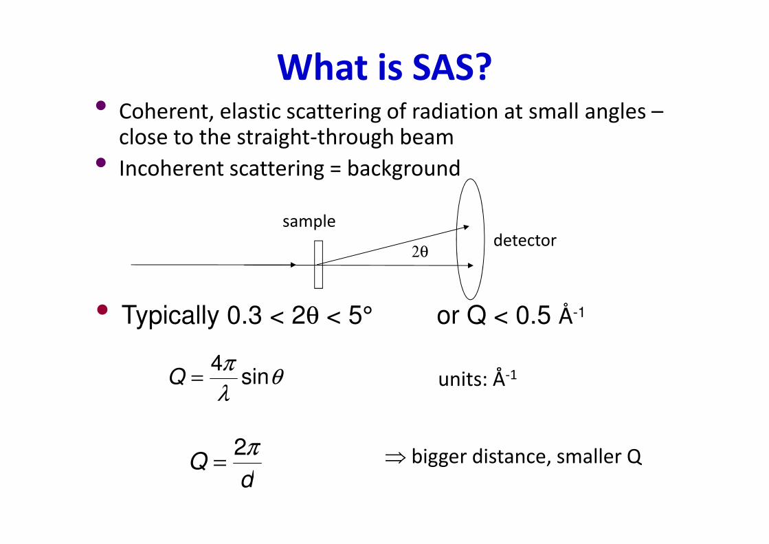
What is SAS?• Coherent, elastic scattering of radiation at small angles –

close to the straight-through beam

• Incoherent scattering = background

2θ

sampledetector

• Typically 0.3 < 2θ < 5° or Q < 0.5 Å-1

θλπ

sin4

=Q units: Å-1

dQ

π2= ⇒ bigger distance, smaller Q

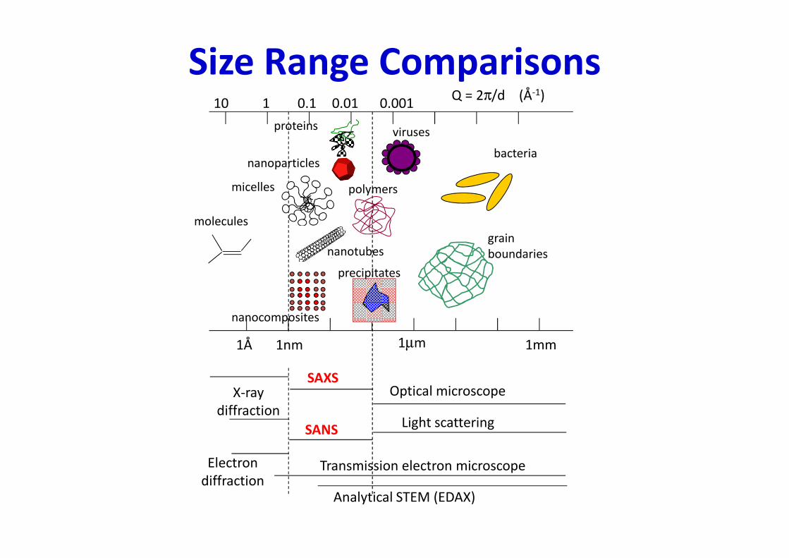
Size Range Comparisons

1Å 1nm 1µm 1mm

Transmission electron microscope

Analytical STEM (EDAX)

SANS

SAXSX-ray

diffraction

Electrondiffraction

10 1 0.1 0.01 0.001

Optical microscope

Light scattering

viruses

bacteria

grain boundaries

polymers

proteins

micelles

molecules

nanocomposites

Q = 2π/d (Å-1)

nanotubes

precipitates

nanoparticles

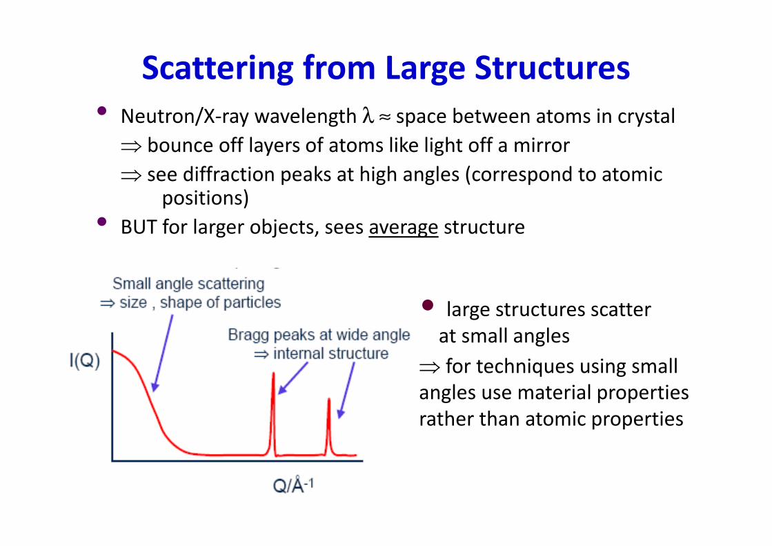
Scattering from Large Structures

• Neutron/X-ray wavelength λ ≈ space between atoms in crystal

⇒ bounce off layers of atoms like light off a mirror

⇒ see diffraction peaks at high angles (correspond to atomic positions)

• BUT for larger objects, sees average structure

• large structures scatter at small angles

⇒ for techniques using small angles use material properties rather than atomic properties

SAS Instruments

So

urc

e

collimation

slits

sample

detector

• Neutrons/X-rays must be parallel to each other; “collimated”• Slit defines shape of beam (circle, square, slit)• Distance from sample to detector & wavelength determines

size range measured Tof – wide simultaneous Q range, lower flux Reactor – smaller Q range, higher flux at short sample-detector

distances

beamstop

q

0.00 0.05 0.10 0.15 0.20

log

I(q

)

0.1

1

10

100

1000

shadow of beamstop

ripples due to polymer structure

radial average:

Real space

detector

• eg diblock copolymers

• Circular 1D average take average over ring

each ring corresponds to one data point in reduced 1D SAXS data

Scattering Patterns: From detector to 1D

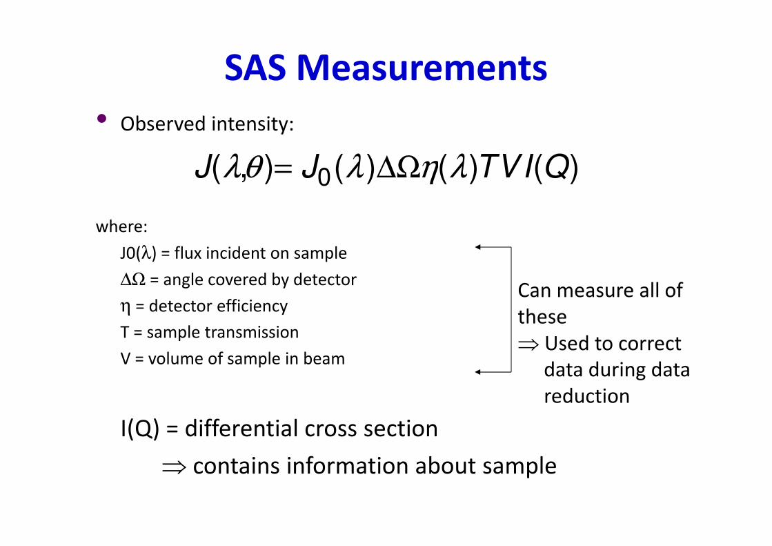
SAS Measurements

• Observed intensity:

where:

J0(λ) = flux incident on sample

∆Ω = angle covered by detector

η = detector efficiency

T = sample transmission

V = volume of sample in beam

I(Q) = differential cross section

⇒ contains information about sample

)()()(),( 0 QIVTJJ ληλθλ ∆Ω=

Can measure all of these⇒ Used to correct

data during data reduction

Sample Scattering

• Measured intensity due to:

Scattering from sample

Scattering from container, slits, air etc

Stray X-rays and electronic noise

Need to measure more than just sample scattering…

Stray radiation & electronic noise

cell

Extra measurements

Source

Scattering from:

1) empty cell

2) windows & collimation slits

3) air scattering

- Minimize air in beam path

- Carefully choose cell & window materials

- Measure an empty cell

Empty cell Blocked beam Detector efficiency

Source

1) Detector dark current2) Stray radiation3) Cosmic radiation

- Measure a blocked beam

Why ?

Sensitivity of each pixel is slightly different (~ 1%)

- Use isotropic scattering material(Plexiglass or water)or “flood” source

Standards - Intensity

• Y-axis in “counts” Need to convert to absolute intensity

• Intensity standards:

water

glassy carbon

direct beam + attenuator (if flux is known)

standard polymer sample

• Scattering cross section (intensity) is known

• Measure intensity of standard under same conditions as sample

• Compare measured and known intensities

• Calculate “scale factor” to multiply data

Scattered Intensity

• observed scattered intensity is Fourier Transform of real-space shapes

where: Np = number of particles

Vp = volume of particle

ρ = scattering length density (of particle/solvent)

B = background

F(Q) = form factor

S(Q) = structure factor

• Sample considerations…

BQSQFVNQI sppp +−= )()()()(22 ρρ

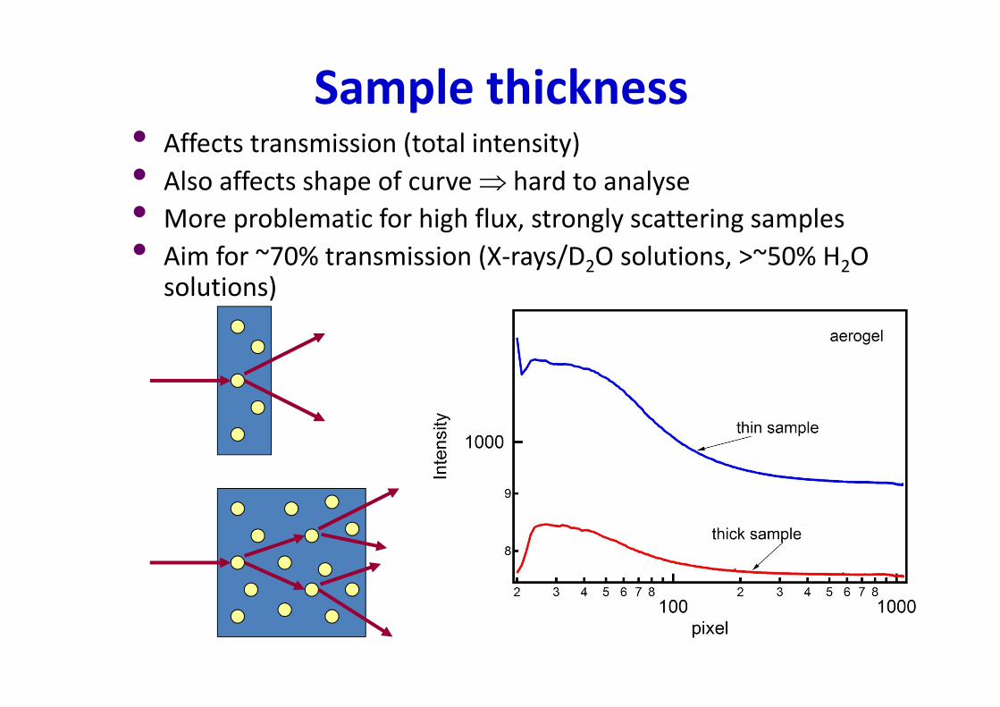
Sample thickness• Affects transmission (total intensity)

• Also affects shape of curve ⇒ hard to analyse

• More problematic for high flux, strongly scattering samples

• Aim for ~70% transmission (X-rays/D2O solutions, >~50% H2O solutions)

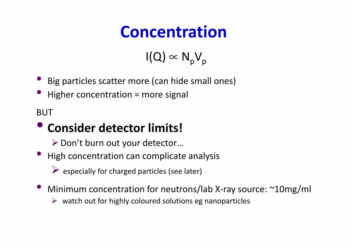
Concentration

I(Q) ∝ NpVp

• Big particles scatter more (can hide small ones)

• Higher concentration = more signal

BUT

• Consider detector limits!Don’t burn out your detector…

• High concentration can complicate analysis

especially for charged particles (see later)

• Minimum concentration for neutrons/lab X-ray source: ~10mg/ml watch out for highly coloured solutions eg nanoparticles

Neutrons/X-rays & “Contrast”• Neutrons more penetrating than X-rays (interact less with matter)

• Interaction of neutrons with nuclei depends on isotope

• Interaction of X-rays just depends on number of electrons

• b = scattering length (units Å or cm, normally)

• Scattered intensity measured depends on which isotopes are in sample for neutrons, only on elements for X-rays

X-rays neutrons

Scattering from Large Structures

• Consider H2O: volume of one molecule = 30Å2

radius of one molecule = 2 Å

⇒ for distances > ~5 molecules, see only average density

Q = 2π/d

• so can use material properties for Q < ~0.6 Å-1

R

R

density

ρav

R=10 Å

Scattering Length Density

• scattering from an object/material depends on how many electrons or nuclei there are in a unit volume

• use scattering length density, Nb, to calculate scattering from molecules:

∑=

∑⋅

=

ii

ii

A

bN

bMW

NNb

ρ

where: bi = scattering length for element, cm(for X-rays b = 2.81×10-13 × no. of e- in atom)

ρ = density of compound, g cm-3

NA = Avogadro’s number, mol-1

MW = molecular weight, g mol-1

N = number density of atoms in material, cm-3

NB/ if feeling lazy see: www.ncnr.nist.gov/resources/sldcalc.html

Units of Nb: cm-2

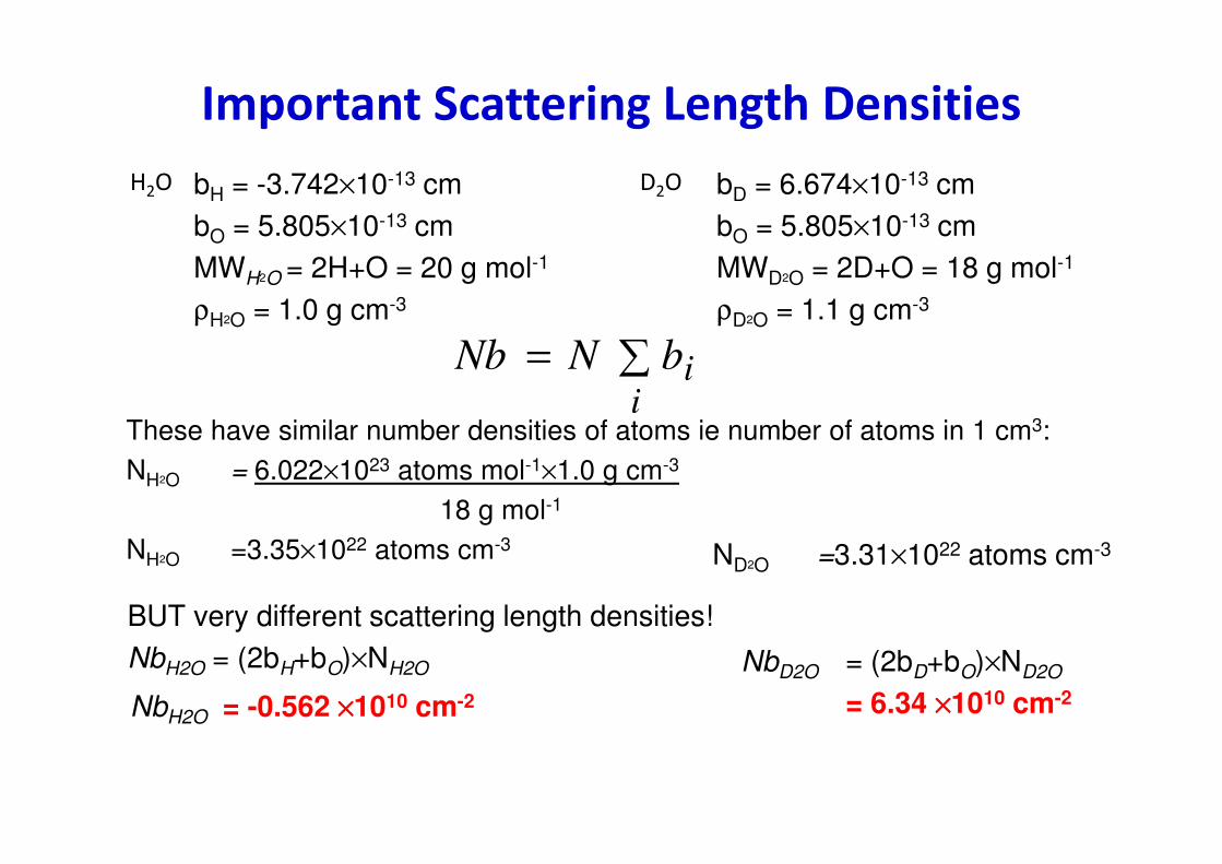
Important Scattering Length Densities

These have similar number densities of atoms ie number of atoms in 1 cm3:NH2O = 6.022×1023 atoms mol-1×1.0 g cm-3

18 g mol-1

NH2O =3.35×1022 atoms cm-3

D2ObH = -3.742×10-13 cm bD = 6.674×10-13 cmbO = 5.805×10-13 cm bO = 5.805×10-13 cmMWH2O = 2H+O = 20 g mol-1 MWD2O = 2D+O = 18 g mol-1

ρH2O = 1.0 g cm-3 ρD2O = 1.1 g cm-3

BUT very different scattering length densities!NbH2O = (2bH+bO)×NH2O

NbH2O = -0.562 ××××1010 cm-2

ND2O =3.31×1022 atoms cm-3

H2O

NbD2O = (2bD+bO)×ND2O

= 6.34 ××××1010 cm-2

∑=i

ibNNb

Contrast & Contrast Matching

• Both tubes contain pyrex fibers + borosilicate beads + solvent.

(A) solvent refractive index matched to pyrex fibres

(B) solvent index different from both beads & fibers – scattering from fibers dominates

2)()( spQI ρρ −∝

Similarly, there must be a difference between object and surrounding to measure scattering

Babinet’s Principle

• These two structures give the same scattering

• Contrast is relative

• Loss of phase information i.e.: is ρ1 > ρ2?

• Very important in multi-phase systems

Solve by use of multiple contrasts using SANS!

(for X-rays = anomalous scattering)

2)()( spQI ρρ −∝

Scattering ∝∝∝∝ “Contrast”• objects and solvent have

different scattering length densities (SLD)

• Intensity ∝ SLD differencebetween solvent & particle

• in water for neutrons can manipulate solvent ρ by using mixture of H2O and D2O

• When solvent and object have same SLD they are said to be “contrast matched”

Example: silica spheres in water

95% D2O in H2O

59% D2O in H2O

30% D2O in H2O

Predicting Contrast Match Point• By calculating the SLD can predict %D2O where

the scattering signal will be zero

• BUT if have exchangeable hydrogens in the structure the SLD will vary with %D2O

Neutron “Contrast” Series• intensity of scattering depends on difference between

particle and solution.

I ∝ (Nbparticle - Nbsolution)2

• measure scattering at a series of solution contrasts

• extrapolate scattering to Q = 0 and measure I0

Contrast Match Point• Plot as √I0 vs [D2O]

• Place where line cuts zero is where the solution has the same scattering length density as the particle⇒ contrast matched

• Can use this to find the density of the particle

Neutron “Contrast” for Complex Objects

• contrast matching allows us to “remove” scattering from parts of an object

25

“shell-contrast”⇒ see only core

“core-contrast”⇒ see only shell

Solvent matching for C0C2-actin assembly• cardiac myosin binding protein C (C0C2) has extended modular structure• Mixing C0C2 with G- actin solutions results in a dramatic increase in

scattering signal due to formation of a large, rod-shaped assembly

Whitten, Jeffries, Harris, Trewhella (2008) Proc Natl Acad Sci USA 105, 18360-18365

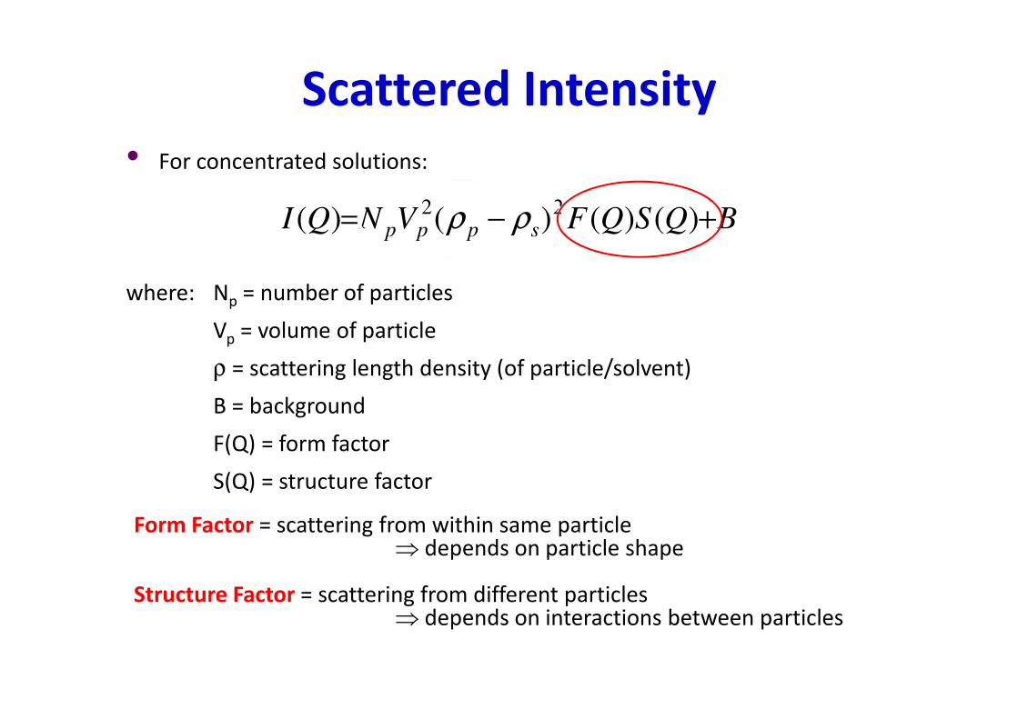
Scattered Intensity

• For concentrated solutions:

where: Np = number of particles

Vp = volume of particle

ρ = scattering length density (of particle/solvent)

B = background

F(Q) = form factor

S(Q) = structure factor

BQSQFVNQI sppp +−= )()()()(22 ρρ

Form Factor = scattering from within same particle⇒ depends on particle shape

Structure Factor = scattering from different particles⇒ depends on interactions between particles

Solution of particles

=

SolutionI(c,Q)

Form factorof the particle

Motif (protein, micelle, nanoparticle)

F(0,Q)

Structure factorof the particle

LatticeS(c,Q)

*

*

c = concentration

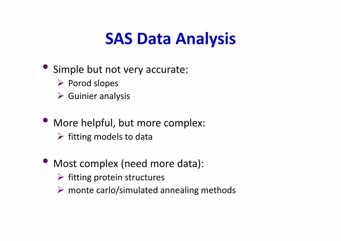
SAS Data Analysis

• Simple but not very accurate: Porod slopes

Guinier analysis

• More helpful, but more complex: fitting models to data

• Most complex (need more data): fitting protein structures

monte carlo/simulated annealing methods

() = Ω = 1

( )

.

Scattering from Independent Particles

• Scattered intensity per unit volume of sample arises from spatial distribution of regions

with different scattering length density

• For identical particles:

() = ( − ) 1

.

V, ρρρρs

Vp, ρρρρp

Particle form factor, F(Q)

Dilute Randomly Ordered Uniform

Particles

• scattering from independent particles:

• Assume: i) system is isotropic, then = !"()

ii) no long range order, so no correlations between two widely separated particles

() = ( − ) 1

.

() = ()( − ) $(%) sin(%)% 4*%%+

,$(%) = correlation function within particle

P(r)=4πr2γ(r) is the probability of finding two points in the particle separated by r

Porod’s Law• Start with form factor:

• Now consider radial pair correlation function for sphere, with sharp edges, radius R:

• Integrate by parts three times:

R

Porod Scattering

• Slope at high q the same

• But point where slope changes depends on particle dimensions

A

B

10% red / 90% blue in each square

Fractal Systems• Fractals are systems that are self-similar as you change scale

• For a Mass Fractal the number of particles within a sphere radius R is proportional to RD where D = fractal dimension

• Thus:

4πR2γ(R)dR = number of particles between distance R and R+dR

= cRD-1dR

Diffusion-limited aggregation in 3 dimensions (Paul Bourke, http://local.wasp.uwa.edu.au/~pbourke/fractals/dla3d/)

Fractal Systems Continued…

•

First stages of Koch (triangle) surface(Robert Dickau)

Paul Bourke

The SANS Toolbox. Boualem Hammouda, NIST

37

Porod Slopes & Structures

eg Silica Gel:continuum network surface

cluster particle atoms

ln(Q)

Q = 1/R

I ∝ Q-D

Q = 1/r

I ∝ Q-Ds-6ln

(Int

ensi

ty)

Si

Si

Rr

NB/ SAXS data, seldom measure such a wide Q range in SANS

Form Factors• Form factors are the sum of scattering from every point inside a

particle

• Simplify to the integral

• Scattering pattern calculated from the Fourier transform of the

Real space d

ensity d

istr

ibution real-space density

distribution

• Pattern for most shapes must be solved analytically

• Some simple shapes can be solved directly

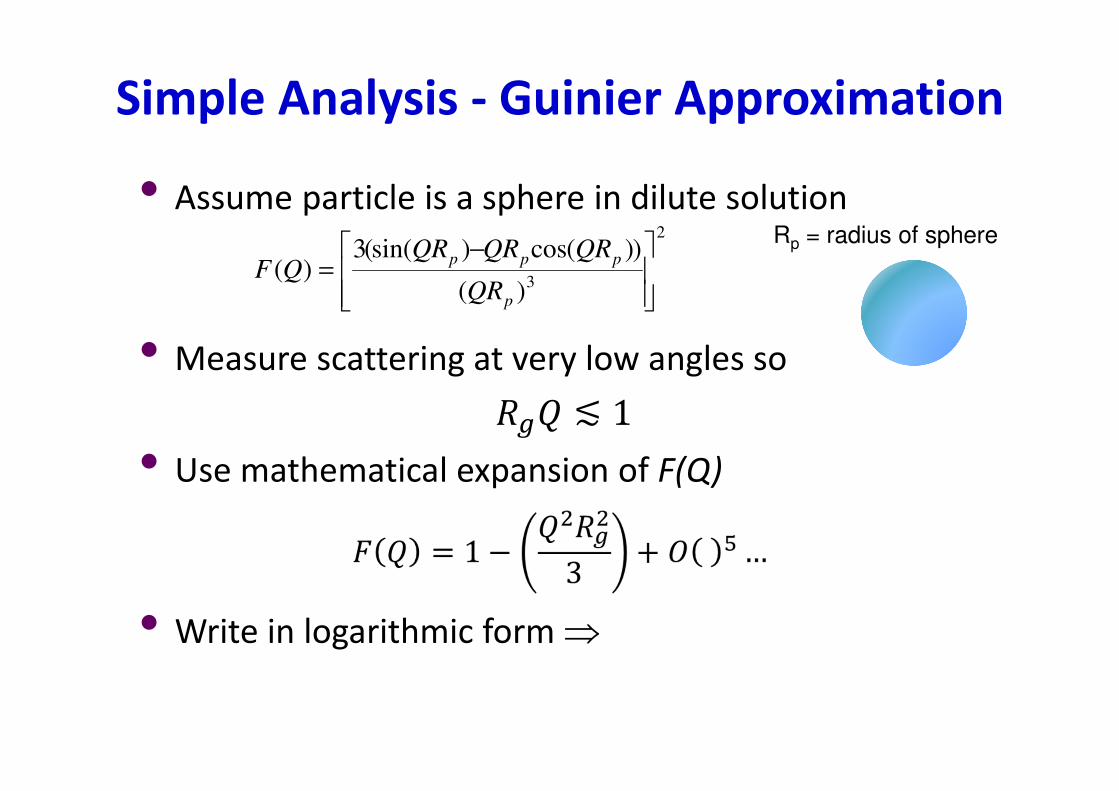
Simple Analysis - Guinier Approximation

• Assume particle is a sphere in dilute solution

• Measure scattering at very low angles so

-./ ≲ 1• Use mathematical expansion of F(Q)

• Write in logarithmic form ⇒

2

3)(

))(cos)(sin(3)(

−=

p

ppp

QR

QRQRQRQF

Rp = radius of sphere

Guinier Plots

• at low concentrations and small values of Q, can write intensity as:

• so plot of ln(I) against Q2 will have slope =

• only valid for RgQ ≤ 1

Radius of Gyration – depends on particle shape

• Sphere

−=

3exp)0()(

22QRIQI

g

3

2gR−

22

53

RRg =R

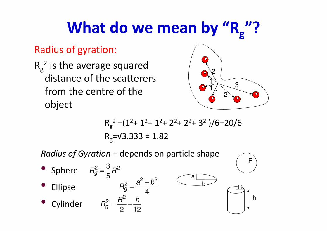
What do we mean by “Rg”?

Radius of gyration:

Rg2 is the average squared distance of the scatterers from the centre of the object

Rg2 =(12+ 12+ 12+ 22+ 22+ 32 )/6=20/6

Rg=√3.333 = 1.82

2

211 1

3

Radius of Gyration – depends on particle shape

• Sphere

• Ellipse

• Cylinder

22

53

RRg =

4

222 ba

Rg+

=

122

22 hR

Rg +=

ab

R

R

h

Slope = = -45.1 Å

so: Rg = 11.6 Å

Guinier Plot Example• Polymerised surfactant micelles Large Scale Structures, ISIS Annual Report, 1999-2000 http://www.isis.rl.ac.uk/isis2000/science/largescale.htm

Q (Å-1) Q2 (Å-2)×10-3

Intensity (cm-1)

ln(intensity)

0.032 1.03 0.127 -2.064

0.050 2.51 0.113 -2.183

0.070 4.87 0.106 -2.245

0.081 6.56 0.096 -2.341

0.095 9.03 0.087 -2.441

0.104 10.81 0.080 -2.528

0.115 13.23 0.073 -2.618

0.123 15.13 0.063 -2.769

0.129 16.64 0.062 -2.7893

2gR−

Check validity: Rg×Qmax = 11.6×0.095 = 1.1 OK

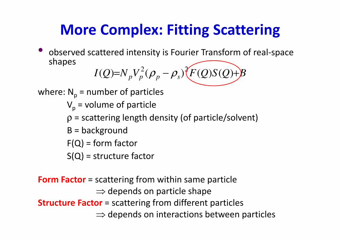
More Complex: Fitting Scattering

• observed scattered intensity is Fourier Transform of real-space shapes

where: Np = number of particles

Vp = volume of particle

ρ = scattering length density (of particle/solvent)

B = background

F(Q) = form factor

S(Q) = structure factor

Form Factor = scattering from within same particle⇒ depends on particle shape

Structure Factor = scattering from different particles⇒ depends on interactions between particles

BQSQFVNQI sppp +−= )()()()(22 ρρ

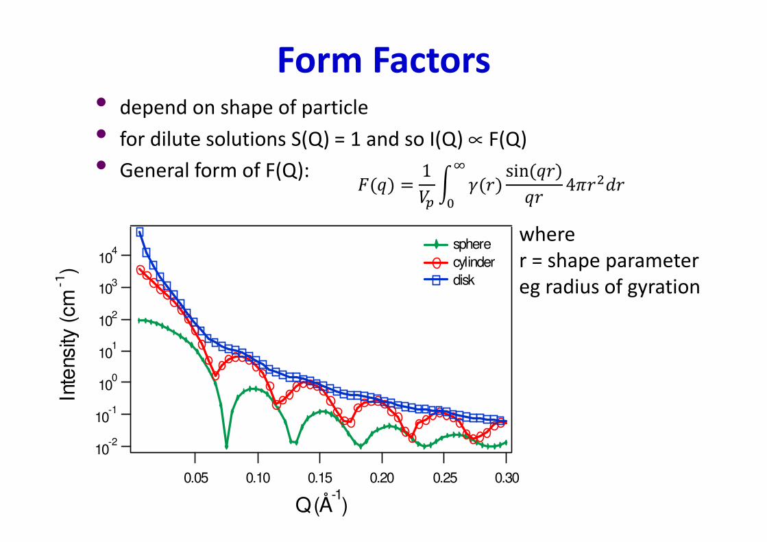
Form Factors• depend on shape of particle

• for dilute solutions S(Q) = 1 and so I(Q) ∝ F(Q)

• General form of F(Q):

10-2

10-1

100

101

102

103

104

Inte

nsity

(cm

-1)

0.300.250.200.150.100.05

Q (Å-1)

sphere cylinder disk

where r = shape parameter eg radius of gyration

Polydispersity• “smears out” sharp features in pattern

• “smearing” can also be due to poor Q resolution or beam shape (correct for this during data reduction)

0.1

1

10

100

1000

Inte

ns

ity

(a

rb u

nit

s)

0.012 3 4 5 6 7 8 9

0.12 3

Q (A-1

)

0.01

0.1

1

10

100

1000

Inte

ns

ity

(a

rb u

nit

s)

0.012 3 4 5 6 7 8 9

0.12 3

Q (A-1

)

0.01

0.1

1

10

100

1000

Inte

ns

ity

(a

rb u

nit

s)

0.012 3 4 5 6 7 8 9

0.12 3

Q (A-1

)

0.01

0.1

1

10

100

1000

Inte

ns

ity

(a

rb u

nit

s)

0.012 3 4 5 6 7 8 9

0.12 3

Q (A-1

)

Au NanorodsFitted to charged cylinders• Radius 104Å• Length 307ÅClearly need to incorporate

polydispersity!

10-6

10-5

10-4

10-3

10-2

10-1

100

Inte

nsity

(ar

b. u

nits

)

2 3 4 5 6 7 8 90.1

2 3

Q (A-1

)

data fit

Fitted to charged cylinders• Radius 80Å• Length 190Å• Polydispersity 0.29

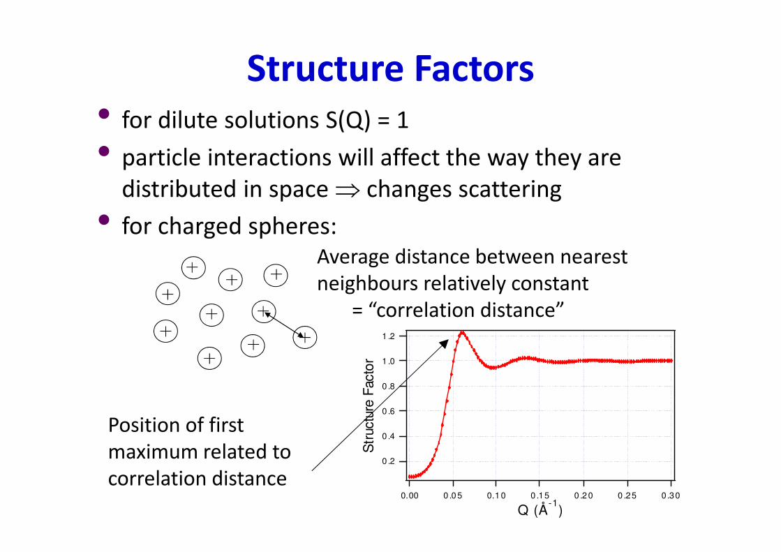
Structure Factors

• for dilute solutions S(Q) = 1

• particle interactions will affect the way they are distributed in space ⇒ changes scattering

• for charged spheres:Average distance between nearest neighbours relatively constant

= “correlation distance”1 .2

1 .0

0 .8

0 .6

0 .4

0 .2

Str

uctu

re F

acto

r

0 .300 .250 .2 00 .150.1 00 .0 50.00

Q (Å-1

)

Position of first maximum related to correlation distance

Concentration effects

Combining F(Q) & S(Q)

• In most cases when fitting will need to include both form and structure factor

• Can tell by taking concentration series

if shape of scattering doesn’t change when sample is diluted then S(Q) = 1

• Polymer-lipid discs

• Normalised for concentration

50

Combining F(Q) & S(Q)

• Use computer programs to combine form factor and structure factor:

• Fit using ellipse + structure factor for charged objects which repel each other ⇒ many parameters!

• Use three contrasts to help pin down shape and size accurately

0.1

2

3

456

1

2

3

45

Inte

nsity

(cm

-1)

7 8 90.01

2 3 4 5 6 7 8 90.1

2

Q (Å-1)

100% D2O 59% D2O 35% D2O

17Å

31Å

+ + ++ +

+

++ + +

+ + ++

++

+

++

+

+ +

+ +

++

Brennan, Roser, Mann, Edler, Chem. Mater. 2002, 14, 4292

Fourier Inversion Techniques• Scattering from dilute, uniform, independent particles

• Assuming i) system is isotropic, then −1/% = sin(/%)/%

ii) no long range order, so no correlations between two widely separated particles

• If can measure I(Q) over big enough range can take inverse Fourier transform to find P(r):

P(r)=4πr2γ(r) =

(/) = (/)( − ) $(%) sin(/%)/% 4*%%+

,$(%) = correlation function

P(r)=4πr2γ(r) is the probability of finding two points in the particle separated by r

2*/ / sin /% /

P(r) for Simple Shapes

• Note: P(r) can be ambiguous if have polydispersesamples

Aggregates = sum of separate shapes

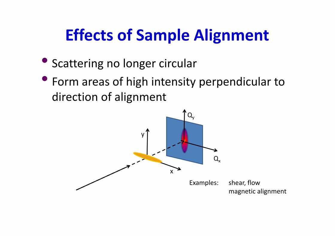
Effects of Sample Alignment

• Scattering no longer circular

• Form areas of high intensity perpendicular to direction of alignment

y

x

Qy

Qx

Examples: shear, flowmagnetic alignment

Isotropic vs Nonisotropic Structures

No shear⇒Isotropic solution

-0.2

-0.1

0.0

0.1

0.2

Qy (Å

-1)

-0.2 -0.1 0.0 0.1 0.2

Qx (Å-1)

-0.2

-0.1

0.0

0.1

0.2

Qy (Å

-1)

-0.2 -0.1 0.0 0.1 0.2

Qx (Å-1)

0.12M CTAB/0.2M KBr 303K shear

-0.2

-0.1

0.0

0.1

0.2

Qy (Å

-1)

-0.2 -0.1 0.0 0.1 0.2

Qx (Å-1)

0.12M CTAB/0.2M KBr 323K

Shear + higher T⇒ isotropic again

Shear⇒ aligned micelles

shear

Edler, Reynolds, Brown, Slawecki, White, J. Chem. Soc., Faraday Trans. 1998, 94(9) 1287

Free SANS Fitting Software

DANSE SANSView software

• Designed for fitting neutron data but can also be used (with care) for X-ray data

• Includes reflectivity analysis

• Available from: http://danse.chem.utk.edu/sansview.html

OR library of other available software at:

http://www.small-angle.ac.uk/small-angle/Software.html